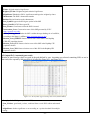
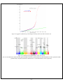
1
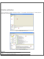
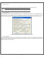
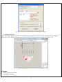
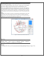
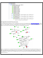
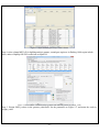
KGG: A systematic biological Knowledge-based mining system for Genome-wide Genetic studies (Version 2.5) User Manual Miao-Xin Li,Hong-sheng Gui Pak C. Sham and You-Qiang Song Department of Psychiatry Department of Biochemistry The University of Hong Kong Pokfulam, Hong Kong SAR, China Content -1- 1. Introduction and general pipeline .................................................................................... 2 2. Installation ...................................................................................................................... 4 2.1 Installation of Java Runtime Environment (JRE) ................................................. 4 2.2 Installation of KGG ............................................................................................... 5 2.3 KGG directory ....................................................................................................... 5 3. Interface and functions .................................................................................................... 6 3.1 Project.................................................................................................................... 7 3.2 Data ....................................................................................................................... 7 3.3 SNP...................................................................................................................... 15 3.4 Gene .................................................................................................................... 19 3.5 Module ................................................................................................................ 25 3.6 Tools .................................................................................................................... 29 4. Input & output files ...................................................................................................... 30 4.1 Input file 1 (GWAS results) ................................................................................ 30 4.2 Input file 2 (Candidate Gene list) ........................................................................ 31 4.3 Output file 1 (log file) ......................................................................................... 31 4.4 Output file 2 (Annotated SNP result) .................................................................. 31 4.5 Output file 3 (Annotated gene result) .................................................................. 32 4.6 Output file 4 (Enriched pathway result) .............................................................. 33 4.7 Output file 5 (Enriched PPI network result)........................................................ 34 4.8 Output file 6 (Graphs in htmllog directory) ........................................................ 35 5. Tutorial .......................................................................................................................... 37 6. Update from KGG 1 to KGG 2.0 .................................................................................. 44 7. References ..................................................................................................................... 45 Hints for large GWAS dataset (around or over 2.5 million SNPs) 1. 2. Maximize your Java heap sizes by –Xmx1500m or a number larger than 1500. Only annotate or export a small set of genes you are interested in by choosing “Gene->Annotate & Export” or “SNP->Annotate & Export”. 1. Introduction and general pipeline KGG (Knowledge-based mining system for Genome-wide Genetic studies) is a software tool to perform knowledge-based analysis for genome-wide association studies (GWAS). At present, it has three major functions, 1) prioritizing SNPs through a knowledgebased weighting method [1]; 2) conducting gene-based association tests using SNP p-values from GWAS[2,3]; 3) advanced biological module-level association analysis (pathway enrichment and protein-protein interaction (PPI) network association) by a set-based test [3] using gene-based p-values. -2- The knowledge-based weighting method for SNPs has described in our paper 1. It combines both biological knowledge and statistical association p-values to produce optimal weights, which can maximize the potential power of association tests while controlling false positive discoveries. The method presents excellent performance in systematical investigations from theoretical calculation, computer simulation and practical application. The gene-based and set-based genome-wide association analysis methods have been described in our paper 2 and 3. These methods do not require the genotypes of SNPs but focuses on quickly combining available statistic SNP p-values for association. Compared with existing methods proposed for gene-based and/or set-based association, a nice characteristic of these methods is that they do not resort to any computation-intensive procedure (like permutation) to address the issue of varied gene/set size (or the number of typed SNPs within a gene/set) and marker dependency. So they have unbeatable speed to handle millions of SNPs while having comparable or/even higher power than existing gene-/set-based methods. KGG currently integrates 8 SNPs- and gene-related biological resources including the SNP annotation from the NCBI dbSNP, pathways and PPI information from multiple databases. 1) SNPs’ gene features (e.g. intron, missense, splicing site, etc.) from dbSNP (http://www.ncbi.nlm.nih.gov/SNP/), 2) conservation scores from the UCSC Genome Browser website (http://hgdownload.cse.ucsc.edu/), 3) positive selection scores of SNPs from http://haplotter.uchicago.edu/selection/, 4) human microRNA target gene binding site information from Sanger’s miRBase (http://microrna.sanger.ac.uk/), 5) disease genes from OMIM (http://www.ncbi.nlm.nih.gov/omim), 6) tissue specific-expression genes from an analyzed dataset of mRNA expression arrays by Greco et al (2008), 7) biological pathways from MsigDB (http://www.broadinstitute.org/gsea/msigdb/index.jsp) and 8) protein-protein interaction information from String database (http://string-db.org/). Files or data involved: GWAS summary results: a file contains SNP-based p values, chi-square statistics or Z-scores see more information of input file in chapter 4. Genome Set: a compiled intermediate dataset, it has integrated original GWAS p-values, SNP annotation and gene annotation, as well as LD information from HapMap reference population or raw genotype data. Candidate Genes & Seed Genes: a list of gene symbols (or gene IDs) from previous GWAS study or Metaanalysis; candidate genes refers to genes with suggestive evidences being involved in the development of the traits or diseases, the seed genes are defined genes with very strong evidence being involved in the development of the traits or diseases according to previous studies. This file is optional; if not offered by user, KGG will automatically select top N significant genes as seed genes ONLY when generating optimal weights for SNPs. SNP-weighted results: weighted p-values for SNPs generated by the algorithm referred in KGG paper 1. Gene-based results: gene-based p-values for statistical association generated by the algorithm referred in KGG paper 2 and 3. PPI Network: PPIs-based p values for association generated by the method described in KGG paper 3. The String PPI (http://string-db.org/) database is used here. Enriched Pathway: pathway-based p values for association generated by the method described in KGG paper 3. The pathway sets from MsigDB (http://www.broadinstitute.org/gsea/msigdb) were used here. Gene Clusters: Subsets of genes which have functional correlations with seed candidate genes of the diseases or traits being studied. This function requires pre-set ‘Candidate Genes & Seed Genes’. Annotated results: significant SNPs or genes with genomic annotations. -3- 2 LD (r-square) of SNPs GWAS results 1 SNP-weighted Results 4 Pathway-Association Results Analysis Genome 7 5 PPI -Association Results 6 Gene Clusters Association Annotated Results Candidate Genes Seeded Genes 3 Gene-Association Results Optional Figure 1.1 Pipeline chart of KGG analysis (version 2.5+) Notes: Circle nodes stand for data and files (input, output); single directional arrows stand for analytical procedures involved. Details for each node and procedure will be given as follows. Steps involved: 1) Build an analysis genome: generate an intermediate dataset which integrates original GWAS p-values, SNP annotation and gene annotation, and LD between SNPs WITIN genes together. It is a unified dataset which will be used for all kinds of analyses on KGG. 2) Weight SNP p-values: produce weighted p-values according to the prior knowledge of tested SNPs by a weighting method[1]. 3) Conduct gene-based association test: calculate gene-based p-values from tested SNPs within or around the genes by GATES[2] or HYST[3]. 4) Explore significantly associated pathways by HYST [3] and enriched with susceptibility genes by hypergeometric distribution test. 5) Explore statistically significant PPI pairs by HYST [3] which may work together to contribute to the development of the disease or traits. 6) Select significant genes in a functional gene set/cluster. Expand a cluster of genes, which share the same pathways or have PPI with seed genes (proposed by users). Genes are separated into two exclusive subsets: the functional cluster and the remainder. Use multiple testing methods to pick up the significant genes in genes in the subsets. 7) Annotate and export significant SNPs, genes, pathways and PPIs. The significant genes are selected according SNP-based p-values, either the original or the weighted. 2. Installation 2.1 Installation of Java Runtime Environment (JRE) The JRE is required to run KGG on any operating systems (OS). It can be downloaded from http://java.sun.com/javase/downloads/index.jsp for free. The version number for KGG is 1.6 or up. Installing the JRE is very easy in Windows OS and Mac OS X. In Linux, you have more work to http://www.java.com/en/download/help/linux_install.xml. do. Details of the installation can be found In Ubuntu, if you have an error message like: “Exception in thread "AWT-EventQueue-0" java.awt.HeadlessException …”, then please installs the Sun Java Running Environment (JRE) first. -4- To install the Sun JRE on Ubuntu(10.04), please use the following commands: sudo add-apt-repository “deb http://archive.canonical.com/ lucid partner” sudo apt-get update sudo apt-get install sun-java6-jre sun-java6-plugin sun-java6-fonts Detailed explanation of above commands can be found at http://www.ubuntugeek.com/how-install-sun-java-runtime-environment-jre-inubuntu-10-04-lucid-lynx.html. For Mac OS, the JRE 1.6 has been available at http://developer.apple.com/java/download/ since April 2008. Mac OS users may need update the Java application to run IGG. A potential problem is that this update does not replace the existing installation of J2SE 5.0 or change the default version of Java. Similar to the Linux OS, the Java_Home environmental variable has to be configured to initiate KGG. Hint: We have prepared a default configure for Mac OS users to change the Java version, in the file, run.mac.sh. 2.2 Installation of KGG KGG has not had an installation wizard by far. After downloaded from our website and decompressed, it can be launched through a command, java -Xms256m -Xmx512m -jar "./KGG.jar”, in a command prompt window provided by OS. In the command, Xms<size> and -Xmx<size> set the initial and maximum Java heap sizes for KGG respectively. A larger maximum heap size can speed up the process of analysis. A higher setting like –Xmx768m is suggested dealing with large number of SNPs, say more than 1,000,000. The number, however, should be less than the size of physical memory. We also prepared three command files, run.linux.sh, run.win.bat and run.mac.sh for the Linux, Windows and Mac OS respectively. In a Microsoft Windows command line terminal, KGG.jar can be initiated by typing “run.win”. In the Linux and Mac terminals, users can type “sh run.linux.sh” and “sh run.mac.sh” to run KGG. Hint: In run.mac.sh, you must ensure the JAVA_HOME is correct in your machine. KGG package downloaded from the website does not include the resource data. You are suggested launching KGG once you download and unzip the KGG package. KGG will automatically download and update the resource data. You will not need to wait for the downloading later when you analyze your data. 2.3 KGG directory After correctly installing JRE and KGG package, the KGG directory should be like Figure 2.1. And x xplanations for file or folder are given as follows: 1) KGG.jar: the main KGG program; 2) kgg.ini.xml: the initiation setting of KGG application; 3) run.linux.sh, run.mac.sh, run.win.bat: example command file for Linux, Mac and Windows respectively; 4) htmlLog folder: intermediate analysis results including figures and log file; 5) lib folder: functional library files of the KGG application; 6) resources folder: TXT files for SNP annotation database, gene annotation database 7) Tutorial folder: store input data for tutorial practice (see chapter 5). Figure 2.1 Structure of KGG directory -5- 3. Interface and functions Once you start KGG, A window will pop up as Figure 3.1.1; the window will be like Figure 3.1.2 when a project is created and executed by KGG. Figure 3.1.1 KGG interface before project Figure 3.1.2 KGG interface after project Illustration: Frame 1: tree-structured branches for different sub-analysis; Frame 2: view of input data or output results; -6- Frame 3: log output of KGG analysis and some results; Frame 4: resources of KGG 3.1 Project Create project: create a new KGG project Open project: open an existing KGG project Latest projects: quickly open one of pervious projects Close project: close the current project Exit: exit the KGG application The first step to use KGG is to create a KGG project. You can click Project->Create Project or the accelerator to open the dialog “Create KGG Project” (Figure 3.2). Figure 3.2: Dialog to create a KGG project Project Name: Project name to identify the project. Project Path: Choose a project path to save analyzed results. Or, you can open a created project anytime you want, which is located as *.xml file in your previous setting directory. Figure 3.3: Dialog to open an existed KGG project 3.2 Data Import original association file Define candidate genes -7- Build analysis genome by RSID Build analysis genome by position 1) Import original association file After the creation of the project, the first thing you need to do is to import your GWAS results (such as output of PLINK). To do this, just click Data->Import original association files or the accelerator . Figure 3.4.1: Dialog to input a GWAS result file Figure 3.4.2: KGG view after GWAS original value input Red box shows a node created by KGG after input, red arrow shows GWAS result. 2) Define candidate genes At the second step, you can define a set of candidate genes of the diseases or traits being studied for the knowledge-based weighting analysis and other functional analysis. Just click the menu Data->Define Candidate Genes to open a “Define Candidate Genes” Dialog. On this dialog, the candidate genes can be defined by three different ways (Input genes by user, select OMIM genes and select Tissue specific genes). To select genes as candidate genes, you need move the selected genes on this table into the bottom table by clicking the “Add” button. Remember that this step is optional; all functions (except for the Functional gene cluster analysis) can go without the definition of candidate genes. However, we suggest using some important candidate genes (if available) -8- as seed genes, which may introduce additional information about the disease into analysis. Figure 3.5: Dialog to directly define the seed candidate genes The second way is to define candidate genes according to OMIM database. The OMIM dataset has been integrated into KGG. You can easily retrieve OMIM genes by the OMIM ID OR disease name on KGG by clicking the “Search” button (Figure 3.6). Retrieved genes can be further selected on KGG by ticking the checkbox on KGG. Please also move selected genes into the bottom table by clicking the “Add” button. -9- Figure 3.6: Dialog to define the seed candidate genes by searching OMIM dataset The third way is to choose tissue specifically expressed genes as the seed candidate genes on KGG (Figure 3.7). These genes were proposed by Greco et al. (2008) [Greco, et al. 2008], where 1601 genes were identified as selectively expressed in one or more human normal tissues. This tissue-specific expression feature might be important for some complex diseases. For instance, genes exclusively expressed in adult brain might be interesting candidates for Alzheimer disease. There are total 77 tissues listed in the top-left table of this dialog. Their selectively expressed genes can be shown on the top-right table by clicking the “View” button. Again, please remember to transfer selected genes into the bottom table by clicking the “Add” button. - 10 - Figure 3.7: Dialog to define the candidate genes by searching tissue specifically expressed genes Genes in the lower table of this dialog are the candidate genes and will be used a reference to generate the optimal weights for the p-values of SNPs or genes or other functional analysis. However, they will be treated differently according to the feature “As Seed”. Genes with the “As Seed” will be set as seed candidate genes to extend a larger set of candidate genes, which share the same biological pathway and having protein-protein interaction with the seed ones, at the beginning of the weighting procedure. When the “As Seed” property is false, the genes will not be used as seed candidate genes to infer others. - 11 - Figure 3.8: Dialog to define candidate gene set and seeded genes Figure 3.9: KGG view after candidate gene set input Finally, you can save the chosen genes in the bottom table into your created project by clicking “Save As” button. A name is required for the candidate gene set to be saved. And a new branch in the frame of ‘projects’ will be created; genes input can also be viewed in the frame ‘data viewer’. 3) Build analysis genome by RSID After the original GWAS result file (include rsID for each SNPs) is imported, you need to build an analysis genome which is necessary for following SNP-based, gene-based, pathway and PPI analysis. Just click the menu Data->Build - 12 - Analysis Genome by RSID or the accelerator to open following dialogue. Figure 3.10: Dialog to set parameters for genome building with RSID Genome Name: genome name prepared for KGG analysis, defined by user; Original association file: Choose a project file to open (if only one files offered, KGG system will auto load this file); select column of p value or chi-square in original GWAS for following analysis; File setting: select chromosome and marker ID column in original GWAS file; Input type include ‘p-values’ and ‘chi-square’, input format contains ‘single test per column’ and also ‘multiple test per column’ (a common format for PLINK output); Exclude regions: some region might include false positive signal or too many noises or outliers; you can remove them at this step. The same LD as available genome: once previous genome was built with LD correction, KGG would store this LD information in the system. Following genome could be easily corrected as long as the same population was used as previous one. LD files & Columns in LD files: KGG offers three different ways for integrating LD information, by HapMap LD SNP coefficients (downloaded from HapMap ftp), genotype of user samples (Plink bed file format) or available local LD SNP coefficients (calculated by third-party tool like Plink). If files for HapMap LD or Local LD - 13 - coefficients are loaded, users also need to define corresponding columns in panel of “Columns in LD files”. 4) Build analysis genome by position If the input association file don’t contain rsID for many variants (see chapter 4 for input file introduction), the analysis genome can be alternatively built by “Build analysis genome by position”. Figure 3.11 shows the frame for setting detailed parameters, and additional annotations not covered in part 3 are also given. Figure 3.11: Dialog to set parameters for genome building with variant position File setting: setting for Marker position column, Marker position version and Reference genome are included in order to correctly map the position on the genome build 18 or 19. Finally, you can click the build button to build a new analysis genome for your original data. It takes some time to run the whole process (you can see it from the log frame if interested). Once finished, KGG will be shown as Figure 3.12. A node named ‘genome set’ will be created, and parameters set for this genome could be viewed by click ‘+’ symbol. - 14 - Figure 3.12: KGG view after genome building; red box shows created node for this analysis 3.3 SNP Weight SNPs Annotation & export 1) Weight SNPs After building genome set, you can start to perform SNP-based analysis now. The “Weight SNPs” dialog (Figure 3.13) can be shown by clicking the menu SNP-> Weight SNPs or the accelerator . Figure 3.13: Dialog to set parameters for SNP weighting Illustration of parameters in Figure 3.13: - 15 - Weight Set Name: define a name of weight set which records the parameters of the weighting procedure; Genome Set: select correct genome set for this analysis (when you have more than one genome sets); Classification Settings: Conservation Score Threshold: A conservation score cutoff to define increased disease risk of SNPs. The range of the score is from 0 to 1. The default cutoff is 0.8. We assume that the higher score, the higher risk. Nature Selection Reference Population: Choose a reference population with nature selection scores. At present, there are only three (CEU, combined HCB and JPT, YRI) available as defined by the HapMap project (http://www.hapmap.org). You can choose just one of populations close to your sample being tested. Nature Selection Score Threshold: A nature selection score cutoff to define increased disease risk of SNPs. The scores are calculated by Voight et al. (2006). Their range is from -∞ to +∞. According to Voight et al. (2006), 2.0 are suggested as the default threshold of significant selection. The higher absolute value of selection score, the more significance of the nature selection and thus the higher risk. The negative scores indicate negative selection; and the positive ones indicate positive selection. Candidate Genes Set: the candidate gene set defined previously; it is optional PPI Level for Candidate Gene Expansion: The exploration depth to extend candidate genes. The default level 2 means that the extended candidate gene set will include genes having indirect PPI with a seed candidate gene. Use Pathway Information: it is optional; once you select it, pathway size can also be limited (default if from 10 to 300 genes per pathway) Weight Settings: Multiple comparison methods: Choose a multiple testing method to calculate significance of tested SNPs; Error Rate: Set the nominal false positive error rate; Top n as the derived seed candidate genes: The top-n (20 is the default number) genes according to the newly weighted p-values are chosen to form a new set of seed candidate genes. Generate weight by iteration: KGG will compute the weighted SNP p-values iteratively according to seed genes; detailed information could be seen in the log frame when KGG is running - 16 - Figure 3.14: KGG view after SNP weighting Finally, you can click the weight button to calculate weighted SNP p-values for your genome set. Once finished, KGG will be shown as Figure 3.14. A node named ‘Weighted SNP Set’ will be created, and parameters set for this genome could be viewed by click ‘+’ symbol. 2) Annotation & Export In the same project you created just now, you can retrieve interesting biological knowledge for SNPs after weighting SNPs. The knowledge may provide important hints for you to understand the statistical significances and propose functional hypothesis. KGG now has four ways to pick up SNPs you are interested in. You can try any one according to your purpose. Figure 3.15.1: Dialog to set parameters for SNP annotated results by p-values - 17 - Figure 3.15.2: Dialog to set parameters for SNP annotated results by SNP ID Figure 3.15.3: Dialog to set parameters for SNP annotated results by genes - 18 - Figure 3.15.4: Dialog to set parameters for SNP annotated results by regions You can check the exported file in your defined output path. See chapter 4 for more information on output file interpretation. 3.4 Gene Association scan; Cluster analysis; Cross validation; Annotation & export LD plot annotation 1) Association scan In parallel with weighting SNP analysis, gene-based association analysis could also performed on the analysis genome built just now. Original p-values will be used to compute gene-based p-values by algorithm referred in KGG paper 2. Multiple outputs will be created, which include Manhattan plots, as well as QQ plots of the gene-based and SNPs-based p-values. Moreover, you can click the ‘Scan’ button to calculate gene-based p-values on the whole genome and check output graphs. Once finished, KGG will be shown as Figure 3.17. A node named ‘Gene Association Set’ will be created, and parameters set for this genome could be viewed by click ‘+’ symbol. - 19 - Figure 3.16.1: Dialog to set parameters for Gene based Scan using the improved Simes test’ method Illustration 1: Scan Name: set a name for this gene-based scan; Genome Set: select the analysis genome built previously; all SNP p-values integrated in the analysis genome will be used Manhattan plot setting: include settings for both gene and SNPs; default threshold for gene is 1E-4 and 1E-6 for SNP. User can reset the thresholds according to the local data. QQ plot setting: include settings for both gene and SNPs; Methods: four different methods are offered----the improved Simes test (GATES), the hybrid set-based test (HYST), the their corresponding weighting versions (details [including the advantages and disadvantages] of the methods are described in the corresponding papers [2,3]) Weight Settings: once ‘the improved Simes test with weights’ selected, setting for ‘conservation score threshold, nature selection score threshold and reference population’ would be shown; The following paragraph illustrates how the weights are constructed. (See illustration 2) Confirmation frame: once ‘all SNPs test’ selected, this frame would pop out and give user some information, usually click ‘Yes’ for following analysis. - 20 - Figure 3.16.2: Dialog to set parameters for Gene based Scan using ‘HYbrid test of extended Simes test [GATES] and scaled chi-square Test (HYST)’ method Figure 3.16.3: Dialog to set parameters for Gene based Scan using ‘The improved Simes test with weights’ method Figure 3.17: KGG view after gene association scan Illustration 2: Construction of weights to prioritize SNPs We used categorical information of available GWAS hits to construct weights for the gene-based test. This is a simple and feasible alternative for the weight construction. Presumably, the weights will reflect a priori likelihood of a particular class of SNP being found to be associated with disease. We downloaded all reported GWAS hits contained in a comprehensive GWAS database (HuGE; - 21 - http://hugenavigator.net/HuGENavigator/gWAHitStartPage.do) (Hindorff, et al., 2009). The number of significant association hits was 2908 as of March 12, 2010. This set was then expanded by including SNPs in strong LD (r20.8) with them in the HapMap database (http://hapmap.ncbi.nlm.nih.gov/). The expanded SNP list was classified into different categories according to their features (See Table 1 for details). The main resource was the the gene-features defined by the dbSNP database (http://www.ncbi.nlm.nih.gov/bookshelf/br.fcgi?book=helpsnpfaq&part=Build.The_dbSNP_Mapping_Pr#Build._Annotation_of_SNPs_t). We summarized the proportion of SNPs belonging to each category among all SNPs of genes which could be slightly expanded by a certain distance, say, 3kb at both sides. We also collected all SNPs which were included by one of the popular 13 Affymetrix and Illumina high-throughput genotyping platforms (including the Illumina HumanHap1M and Affymetrix GenomeWide_Human_SNP_Array_6.0). The number of unique SNPs was 1,778,780. The SNPs were also partitioned into various categories indicated by Table 1. Similarly, we counted the proportion of SNPs of genes in these defined categories. The latter proportions were regarded baselines. The ratio of the proportion of GWAS hits to the proportion SNPs in the genotyping platforms at each category was calculated. Table 1 Criteria to Categorize SNPs utr-5 I: According to gene features where SNPs are located Description Beyond 2 Kb 5′ or 500 bp 3′ but less than x bp of a gene. The default value of x is 3 b. Users can customize it. Within 2 Kb 5′ of a gene (on either strand), but the variation is not in the transcript for the gene Within 500 bp 3′ of a gene (on either strand), but the variation is not in the transcript for the gene In the intron of a gene but not in the first two or last two bases of the intron In the 5′ transcript of a gene but will not be translated utr-3 In the 3′ transcript of a gene but will not be translated 6 codingsynonymous splice-5 Wit in the coding region of a gene but does not change amino acid sequences of a gene In the first two bases of the 5′ intron 7 Feature adjacent near-gene-5 near-gene-3 intron Categories 1 2 3 4 5 8 splice-3 In the last two bases of the 3′ intron 9 missense Within the coding region of a gene and changes amino acid equences of a gene Insertion or deletion disrupting the reading frame/mutations resulting in a premature stop codon 10 frame-shift/ nonsense 11 II: According to non-gene properties If [UCSC Conservation Score >= X (0.8 as default)], then move it to next category If [Selection Score >= Y(2.0 as default)], then move it to next category If [miRNA binding site], then move it to next category The following table (Table 2) shows the ratios according to the three HapMap samples. Although the magnitudes of ratio in the three different HapMap samples are not exactly identical at each category, the general trend is consistent. For example, the Category (C.) 4 has a ratio less than 1 for all the three samples. This makes sense because most of the SNPs in C.4 belong to the introns of genes. Biologically, the introns SNPs may be not as functionally important as other SNPs of a gene, say the coding- synonymous SNPs mainly indicated as C.7. A somewhat unexpected point is the ratio at C.11, which is mainly made up of genomic variants like frame-shift or nonsense. The GWAS hits do not enrich in this category although they might have large biological impact once mutated. One possible explanation is that nonsense polymorphisms we observed as SNPs may not excessively contribute to the development of common complex diseases. This is different from what we learned from the study of Mendelian disorders (Altshuler, et al., 2008; Antonarakis and Beckmann, 2006). The weight for a category is equal to 10Ratio, which will be standardized to make the summation of the weights equal to the SNP number within a gene being tested. In this way, the ratios of the lowest weight to the largest weight are 1:5.05, 1: 3.62, and 1:6.85 for the three HapMap - 22 - populations: CEU, CHB + JPT, and YRI. They could roughly cover the “effective” region we observed in the empirical simulation (see more in the result section). Table 2 Ratios of SNP proportions at each category for the GWAS hits expanded according to three HapMap samples CEU CHB+JPT YRI C.1 1.041 1.026 1.166 C.2 1.244 1.137 1.274 C.3 1.429 1.347 1.431 C.4 0.784 0.831 0.733 C.5 1.363 1.311 1.383 C.6 1.185 1.254 1.024 C.7 1.258 1.200 1.442 C.8 1.487 1.144 1.087 C.9 1.239 1.224 1.569 C.10 0.778 0.788 1.167 C.11 0.884 0.936 0.958 2) Cluster analysis Cluster analysis is used to examine significant genes in a set of candidate genes defined by users. Optionally, user can expand seed genes in the candidate gene set by including genes sharing the same pathway or having PPIs with the seed genes. Detailed explanation for each parameter could be referred in the part of Weight SNPs or gene association scan. Figure 3.18: Dialog to set parameters for Group and cluster gene association 3) Cross validation; If more than one gene-based association p-value sets based on samples were created, cross validate gene association can be used to examine significant genes appear in multiple samples. Increasing evidences of significance could increase the likelihood of being a true association. - 23 - Figure 3.19: Dialog to set parameters for cross validate gene association 4) Annotation & Export As similar to weight SNP annotation & export, association gene scan results can also be annotated and exported, but only by p-values threshold and genes. Figure 3.20.1: Dialog to set parameters for cross validate gene association - 24 - Figure 3.20.2: Dialog to set parameters for cross validate gene association 5) LD plot annotation Once the analysis genome was built with integration of LD information, KGG provides a LD plot for presenting the gene level p-value, the SNP level p-values as well as the LD structure across the variants (see Figure 3.21). Figure 3.21: Dialog to set parameters for LD plot annotation 3.5 Module Pathway-based association PPI-based association - 25 - In the higher level of biological knowledge, KGG provides currently pathway and PPI-based association analysis. More biological module-based analysis methods may be added in the future. The pathway-based association analysis aims to explore enriched and associated pathway (in MsigDB pathways, a secondary pathway dataset curated from KEGG, Reactome, Biocarta database, etc.) by significant genes or seed genes; PPI-based association (protein-protein interaction) analysis aims to explore significantly associated PPIs (in the integrated PPI databases) for a disease in question. 1) Pathway-based association scan Figure 3.22.1: Dialog to set parameters for pathway-based association analysis Each pathway will be interrogated by two tests for their implication to the disease/trait in question: HYST[3] and hypergeometric distribution test[1]. The HYST combines all gene-based p value for association with correction of LD between genes while the hypergeometric distribution test examine statistical significance of enrichment in the pathway by gene with promising p values and pre-set important candidate genes of the disease/trait. The pathways will be sorted according to the summation of the ranks of the two tests. Illustration of parameters in Figure 3.22.1 Exploration Name: set a name for this pathway enrichment exploration; Gene Association Set: available gene-based association results; - 26 - MsigDB pathway: pathway datasets http://www.broadinstitute.org/gsea/msigdb; provided by MSigDB, Pathway size: exclude pathway with too few and too many genes. Statistics: parameters for how to select genes into pathways for hypergeometric distribution test. LD files: The LD data to account for correlation between nearby genes on the same chromosome. Note the built analysis genome only contains LD of SNPs within genes. Export: the path and format to export pathway enrichment results Finally, you can click the ‘Explore’ button to perform pathway enrichment exploration. Once finished, KGG will be shown as Figure 3.23. A node named ‘Enriched pathways’ will be created. Pathway enriched can be viewed from ‘Data view’ frame. You can also check the output result file (Excel or TXT format) from your defined output path. See more from Chapter 4 on output files. Figure 3.23 KGG view after pathway enrichment exploration Red arrow shows enriched pathway, which could also be viewed by internet after right clicked. 2) PPI-based association scan Genes are combined using PPI as analysis units for set-based association test by HYST[3]. Statistically significant PPI pairs and involved genes will be reported. This function has potential to detect genes with moderate effects which normally cannot pass the multiple test using SNP-based and/or gene-based p values. - 27 - Figure 3.24 PPI Association scan setting in KGG Illustration: Scan Name: give a unique name for PPI association scan; Gene Association Set: select one gene-based analysis set previous done, which produced gene level test statistics and p-values; PPI DB: the PPI String database (http://string-db.org/).; PPI DB in File: the customized PPI dataset in a text file. PPI-pair association test: choose to use either HYST or HYST with prior weights in the analysis. The weights were derived from a number of properties of the genes in the PPI network (unpublished data), implying their tendency of being a susceptibility gene of complex diseases. Note: while the result of HYST will be reliable as we declared in [3] the paper , you may only try the HYST with prior weights (unpublished method) to see how it works in your dataset currently. - 28 - Multiple testing by: methods of multiple testing for PPI-based p-values; Keep PPI-pair Heterogeneity: Exclude significant PPI pairs in which the gene-based p values are significant different, in this case there is usually only true susceptibility gene which is highly significant and dominated the resulting PPI-based p value. Always keep significant PPI-pair in which both genes are genome-wide significant: The heterogeneity test may exclude the PPI pairs in which one gene has extremely significant p value and the other has significant p values although both are genomewide significant. After the filtration of heterogeneity test, KGG will get back these PPI pairs. LD files: The LD data to account for correlation between nearby genes on the same chromosome. Note the built analysis genome only contains LD of SNPs within genes. Export: KGG could output PPI association scanning results in local disk, and also automatically pop out the results by PPI viewer (Figure 3.25). Figure 3.25 KGG view after PPI association scan Illustration: Selected Models: include three models, as ‘transforming’, ‘picking’ and ‘annotating’; Layout: include 7 modes of layout, as ‘KKlayout’, ‘FRlayout’, ‘FRlayout2’, ‘Circlelayout’, ‘Springlayout’, ‘Springlayout2’ and ‘ISOMlayout’. 3.6 Tools Currently, KGG offers a tool for automatically downloading HapMap LD data (see Figure 3.26). - 29 - Figure 3.26 KGG tool frame—download HapMap linkage disequilibrium data 4. Input & output files 4.1 Input file 1 (GWAS results) KGG focuses on the downstream analysis of GWA studies, where statistical association p-values (or chi-square values) at SNPs have been generated by conventional statistical genetic methods (such as PLINK). Therefore, the association p-values are the major input of our KGG. KGG flexible supports a user-customized format for the association p-values. Once three columns of information, chromosome number and SNP IDs (or physical position) and p-values are available in a file, you can define the column order by yourselves on KGG. The input file can include more than one p-value column. The following is an example. Example input format (with rsID) of KGG: CHR 4 4 4 4 4 … SNP rs1513559 rs294755 rs835316 rs1841043 rs11726946 … P-value1 0.02301 0.4384 0.002688 0.01115 0.005892 … - 30 - P-value2 0.8815 0.9575 0.007688 0.006112 0.4893 … P-value3 0.007688 0.006112 0.4893 0.119 0 … … … … … … … … Example input format (with only position) of KGG: SNPID Snp1 Snp2 Snp3 Snp4 Snp5 … CHR 4 4 4 4 4 … SNPPOS 100001 110011 120001 130011 140001 … P-value1 0.02301 0.4384 0.002688 0.01115 0.005892 … P-value2 0.8815 0.9575 0.007688 0.006112 0.4893 … P-value3 0.007688 0.006112 0.4893 0.119 0 … … … … … … … … Moreover, a p-value column could include values of different models. KGG will recognize this format if you select the input format as “multiple tests per column” when building the analysis genome. Example a more complex input format of KGG: CHR 4 4 4 4 4 … SNP rs1513559 rs1513559 rs1513559 rs1841043 rs1841043 … P-value1 0.02301 0.4384 0.002688 0.01115 0.005892 … Test-Mode additive recessive dominant additive recessive … P-value2 0.007688 0.006112 0.4893 0.119 0 … … … … … … … … 4.2 Input file 2 (Candidate Gene list) Candidate genes could be loaded one by one or imported from a TXT file. The input file has only one column without header, while one row contains one gene (symbol or ID). 4.3 Output file 1 (log file) All the output in log frame will be saved in log.html file (htmlLog directory). Detailed information of how the analyses are conducted on KGG is recorded in this log file. 4.4 Output file 2 (Annotated SNP result) Results of weighted SNP are saved in the path defined by user. Once opened by text editor, it looks like following graph. Figure 4.1 Txt format of weighted SNP result Illustration of column in the file: - 31 - SNP: RS ID of SNPs in dbSNP PValue: Original statistical significance Weighted_PValue: Weighted original statistical significance. IsSignificant: Whether the SNP is significant according to the weighted p-vlaues Chromosome: The SNPs’ chromosome number Position: Physical location on the chromosome Gene_Symbol: Approved official gene symbol of the SNP Entrez_GeneID: NCBI’ Entrez gene ID. Gene_Feature: Gene feature where the SNP is located Conservation_Score: Conservation score of this SNP generated by UCSC (http://genome.ucsc.edu/). miRNA_Binding_Site: Whether the SNP is within the target binding site of a miRNA, according to the Sanger’s miRBase (http://microrna.sanger.ac.uk/). Selection_Score_CHBJPT: Nature selection score of this SNP in the HapMap CHB+JPT population chosen. Selection_Score_CEU: Nature selection score of this SNP in the HapMap CEU population chosen. Selection_Score_YRI: Nature selection score of this SNP in the HapMap YRI population chosen. 4.5 Output file 3 (Annotated gene result) Results of gene-based p-values are saved in the path defined by user. Assuming user selected containing SNPs or not in the result, once opened by Microsoft Excel, it looks like Figure 4.2.1 and Figure 4.2.2. Figure 4.2.1 Excel format of gene-based p-value result (SNP included) Gene_Symbol: official gene symbol in NCBI; Gene_PValues: gene-based p-values, combined from several SNPs within and around it; IsSignificant: whether significant or not according to a p-value threshold for multiple testing; - 32 - Entrez_GeneID: gene ID recorded by NCBI Entrez; Chromosome: chromosome of the gene Start_Position: start physical position of the gene Length: length of the gene by base-pairs; SNP: SNP ID (rs ***) contributed to the gene; Position: physical location of the SNP; Gene_Feature: SNP’s functional region related to the gene; Conservation_Score, miRNA_Binding_Site, Selection_Score_CHBJPT, Selection_Score_CEU, Selection_Score_YRI: please see the illustration for output file 2; SNP P: p-value for the SNP Figure 4.2.2 Excel format of gene-based p-value result (SNP excluded) Note: the illustration for columns are similar to result file include SNPs, except ‘#SNP’ which means numbers of SNPs of the gene. 4.6 Output file 4 (Enriched pathway result) The shared pathways are presented by a tree structure. Pathway sources, names, involved genes and SNPs are nicely visualized in a hierarchical tree (Figure 4.3). The p-value of the pathway sharing is calculated according to hyper-geometric distribution or our method. - 33 - Figure 4.3 Visualization of shared pathways 4.7 Output file 5 (Enriched PPI network result) The enriched PPI sub-networks are nicely visualized by an open source Java package Jung (http://jung.sourceforge.net/) (Figure 4.4). It is a directed graph. The genes of selected SNPs are the starting nodes. The end nodes are the seed candidate genes. The depth of a sub-network is the largest number of edges from a starting node to an end node. (b) (a) (c) Figure 4.4: Visualization of 2-level sub-PPI network enriched by both seed candidate genes and genes with significant SNPs through our tool KGG. Each node denotes a gene labeled by “Gene Symbol”. The edge indicates a PPI between two genes. The red and green nodes denote tested genes with significant SNPs and seed candidate genes respectively. Here the “2-level” means that the minimal length from a tested gene to a seed candidate gene is 2 (edges). There are intermediate genes (in gray on the plot) between the tested gene and seed candidate genes, which have PPI with the both. - 34 - 4.8 Output file 6 (Graphs in htmllog directory) When running KGG, some graphs as one of the results will automatically be saved in the htmllog directory. These graphs include QQ plots and Manhatton plots for SNPs,genes or PPI networks. It can help user to easy understand and interpret those SNP-based and gene-based analysis done by KGG. Some examples are given as following three graphs. Figure 4.5.1 QQ plot of three sets of SNP p values after weighting SNP analysis Figure 4.5.2 QQ plot of gene-based p-values and the original SNP p-values after gene association analysis - 35 - Figure 4.5.3 QQ plot of PPI-based p-valuesand gene-based p-values after PPI association scan Figure 4.6.1 Manhattan plot of gene-based p values (chr 9 to 22) Note: User can determine to label how many genes and SNPs on the plot by setting different p-value thresholds. In order to present the whole genome clearly, two plots are drawn for chromosome 1 to 8, and chromosome 9 to 22, respectively. - 36 - Figure 4.6.2 Manhattan plot of SNP (around or fell into genes) p values (chr 9 to 22) 5. Tutorial Step 1: create a new project, named ‘CrohnDisease’, and set the project path at C:\KGG\tutorial (or other path defined by user). - 37 - Figure 5.1 Create project Step 2: select the menu Data>Input original association file, choose ‘CrohnGWASresult.txt’ file which contains the whole-genome association p-values for Crohn diseases at SNP-level. This dataset was downloaded from a public domain released by (Barrett, et al., 2008). It includes 7 columns, as SNP, CHR, POS, RISK, NONRISK, META-Z and META-P. Figure 5.2 Input GWAS original result file Step 3: import file ‘CrohnCandidateGeneSet.txt’ as input of candidate gene; define ATG16L1, CARD9, IBD5, IL23R, NOD2 and TNFSF15 as seed genes. Then, save it as candidategeneset_crohn. - 38 - Figure 5.3 Input candidate gene set for crohn’s disease Step 4: select column META-P for building analysis genome; extend gene region to its flanking 10 kb region in both sides; and use HapMap LD SNP coefficients to adjust LD. Figure 5.4 Select META-P to build analysis genome and name the genome as genome_crohn Step 5: Weight SNPs p-values in the genome_crohn built. Set the parameters as Figure 5.5; and name the result as weight_crohn. - 39 - Figure 5.5 Setting for weight SNPs analysis Step 6: export the weight SNPs result by p-value threshold, and save it to local computer with Excel format. Figure 5.6 Annotate weighted SNPs by p-values Step 7: do a gene-based scan using SNP p-values integrated in the analysis genome named genome_crohn, select ‘the GATES (More powerful for a gene with one or a few independent causal variants’ method. Set the parameters as Figure 5.7; and name the result as genescan_crohn. Remember that exported Manhattan plots and QQ plots will be saved in htmlLog folder. - 40 - Figure 5.7 Setting for gene-based scans Step 8: select genescan_crohn as subject, perform cluster analysis for candidate seed genes and their expanded genes (by pathway or PPI network); export the clustering result to local computer by Excel format. Figure 5.8 Setting for group and cluster gene association Step 9: select genescan_crohn as subject, export the gene association results (no need SNP information) to local - 41 - computer by Excel format. Figure 5.9 Annotate gene-based association result by p-values Step 10: perform pathway enrichment exploration both by gene p-values; settings as Figure 5.10. - 42 - Figure 5.10 Pathway enrichment exploration by gene p-values Step 11: search PPIs between significant genes. The significant genes can be picked up according to the gene p-values and SNP p-values; set as Figure 5.11. - 43 - Figure 5.11.1 PPI association scan by gene-based p-values Step 12: View results of Crohn’s Disease By text file or Excel file Open text or excel file for snp-based or gene-based analysis from local computer By Graphs Check QQ plots and Manhattan plots saved in htmlLog folder By KGG Interface Visualize pathway and PPI network output on KGG interface. 6. Update from KGG 1 to KGG 2.0 - 44 - Much progress was made from KGG 1.0 to KGG 2.0, mainly illustrated as follows: 1) Include gene-based analysis; 2) More structured design; 3) Less computation burden; 4) Outputs from KGG are more illustrative and easily interpreted. 7. References 1. Li MX, Sham PC, Cherny SS, Song YQ. A knowledge-based weighting framework to boost the power of genome-wide association studies. PLoS One. 2010 Dec 31;5(12):e14480. 2. Li MX, Gui HS, Kwan JS, Sham PC. GATES: A rapid and powerful gene-based association test using extended Simes procedure. Am J Hum Genet. 2011 Mar 11;88(3):283-293. 3. Li MX*, Kwan JS*, Sham PC. HYST: A hybrid set-based test for genome-wide association studies, with application to protein-protein interaction-based association analysis. Am J Hum Genet. Am J Hum Genet. 2012 Sep 7;91(3):478-88. - 45 - - 46 -