Download Global Map Raster Devel- opment (GMRD) Tool User`s Manual

Global Map Raster Development (GMRD) Tool
User’s Manual
Index
1.
Introduction ............................................................................................................................ 1
1-1. Abstract .............................................................................................................................. 1
1-2. Requirements ..................................................................................................................... 1
1-3. Operating Environment..................................................................................................... 2
1-4. Creation Date..................................................................................................................... 2
1-5. Copyright ........................................................................................................................... 3
2.
Installing Software ................................................................................................................. 4
2-1. Preparing to Install Required Software ............................................................................ 4
2-2. Installing GRASS............................................................................................................... 4
2-3. Installing OSGeo4W ........................................................................................................ 11
2-4. Installing pyModis ........................................................................................................... 15
2-5. Installing Statistical Package R ...................................................................................... 18
3.
Pre-processing Satellite Images ........................................................................................... 25
3-1. Setting up the GRASS Environment............................................................................... 25
3-2. Setting the Environment Variables Used for Executing Scripts .................................... 32
3-3. Downloading MODIS Data .............................................................................................. 34
3-4. Reprojecting and Merging Images................................................................................... 39
3-5. Importing GeoTIFF Images into GRASS ........................................................................ 40
3-6. Managing Intermediate Data .......................................................................................... 44
3-7. Limiting Analysis Extent with a Mask ........................................................................... 45
3-8. Removing Cloud Cover .................................................................................................... 52
3-9. Processing Landsat images ............................................................................................. 55
3-10. Processing VIIRS images ............................................................................................... 62
4.
Creating a Land Cover Map ................................................................................................. 68
4-1. Acquiring Training Data for Your Image Classification ................................................. 68
4-2. Importing Training Data into GRASS ............................................................................ 72
4-3. Calculating Various Indices ............................................................................................ 74
4-4. Verifying Training Data .................................................................................................. 76
4-5. Classifying Land Cover.................................................................................................... 77
4-5-1. Grouping Images for Supervised Classifications ...................................................... 77
4-5-2. Classifying Images Using the Maximum Likelihood Classifier ................................ 78
4-5-3. Classifying Land Cover Using the Decision Tree Method ........................................ 82
4-6. Checking Classification Results ...................................................................................... 84
4-7. Reclassifying raster values .............................................................................................. 85
4-8. Resampling Images.......................................................................................................... 88
4-9. Generating random verification points ........................................................................... 88
4-10. Evaluating a Classification Accuracy using Verification Data ..................................... 93
4-11. Exporting the Land Cover Map ..................................................................................... 96
5.
Estimating Percent Tree Cover Using the Land Cover Map............................................... 98
5-1. Aggregating Indices within Training Areas .................................................................... 98
5-2. Creating Training Data for the Image Classification ..................................................... 99
5-3. Running a Decision Tree Model .................................................................................... 101
5-4. Estimating Percent Tree Cover ..................................................................................... 103
5-5. Combining the Prediction Images and Creating a Tree Cover Image.......................... 103
5-6. Matching Spatial Resolution to Fit the Global Map Standard ..................................... 104
5-7. Excluding Open Water Areas from the Analysis .......................................................... 105
5-8. Assessing Accuracy with Random Points ...................................................................... 109
5-9. Exporting the Tree Cover Map ...................................................................................... 113
6.
Tips and References ............................................................................................................ 116
Classifying Land Cover Type................................................................................................. 116
Developing Training Data for the Tree Cover Map .............................................................. 116
Estimating Percent Tree Cover ............................................................................................. 116
FAQ............................................................................................................................................ 118
Software Installation and Environment Settings ................................................................. 118
General Environment Settings and Data Download ............................................................ 120
Individual processes .............................................................................................................. 120
Software licenses.................................................................................................................... 125
Appendix .................................................................................................................................... 127
A-1. Developing a Tree Cover Map with See5/Cubist ........................................................... 127
1. Creating sub-regions ...................................................................................................... 127
2. Executing the modis_extract_dn.sh by masking the sub-regions ................................. 128
3. Creating random points ................................................................................................. 128
4. Adding attribute fields to the random point map .......................................................... 129
5. Exporting the table......................................................................................................... 130
6. Editing the .data and .names files ................................................................................. 131
7. Executing See5 and Cubist ............................................................................................ 132
8. Importing calculated results .......................................................................................... 132
9. Importing calculated results from Cubist ...................................................................... 133
10. Integrating results by group ........................................................................................ 135
A-2. Program references ........................................................................................................ 136
1. Introduction .................................................................................................................... 136
2. Pre processing................................................................................................................. 137
3. Creating land cover maps .............................................................................................. 150
4. Calculating Percent tree cover ....................................................................................... 162
1.
Introduction
1-1.
Abstract
This Manual is designed to assist you in developing land cover and percent tree cover layers using satellite images. It includes detailed explanations that will allow you to create Global Map
products using satellite images collected by the Moderate Resolution Imaging Spectroradiometer
(MODIS) mounted on the Terra and Aqua satellites, Landsat8, and the Visible Infrared Imaging
Radiometer Suite (VIIRS) mounted on the Suomi National Polar-orbiting Partnership (Suomi
NPP) satellite. The following chapters include instructions on how to:

Obtain and install open-source desktop GIS software (Chapter 2)

Download and preprocess data for image analysis (Chapter 3)

Develop land cover data using satellite images (Chapter 4)

Develop percent tree cover layers using the land cover data and satellite images (Chapter 5)

Find reference documents and analysis tips (Chapter 6)
You will run various shell scripts for the above processes. You can find all the scripts you will
use in the “/script” folder of the CD-ROM provided with this Manual. We assume users of this
Manual are already familiar with basic satellite image analysis as well as data handling with geographic information system (GIS) software.
1-2.
Requirements
This Manual is designed for people who have basic knowledge and skills in the following fields:

Geographic coordinate systems and map projection

Image formatting and processing

Remote sensing technology

Windows operating system
This Manual does not give detailed explanations about the above-mentioned items. Please refer
to other documents if needed.
1
1-3.
Operating Environment
We developed and tested all scripts in a Microsoft Windows 7, 64-bit environment. The programs discussed in this Manual do not require your personal computer (PC) to have any particular
specifications in order to run them properly. However, you will want to ensure that the various required software work normally on your PC. If you purchased your PC recently (2012 or later), you
shouldn’t have a problem running the scripts we provided. You will, however, need sufficient hard
disk space to store satellite images (about three times the size of your original satellite images), as
well as intermediate and final products. Below are the specifications of the lower-end PC we used
to test all scripts.
Processor: AMD Athlon™ II X2 250 Processor 3.00 GHz
Memory: 4 GB
Hard disk space: 256 GB
Graphic card (no requirement): ATI Radeon HD 4200
Operating System: Windows 7, SP1
We also tested our scripts under a Windows7, 32-bit environment.
Processor: Intel Xeon E5420 2.50 GHz 2 Processor
Memory: 4GB
Hard disk space: 256GB
Graphic card (no requirement): VGABIOS Cirrus extension
Operating System: Windows 7 Enterprise
Some of the programs in this Manual require a large amount of memory. Thus, scripts may
stop working in the middle of the process because of the lack of free memory space. In that case,
you may need to close other running software on your PC or narrow your analysis extent.
1-4.
Creation Date
2
We wrote this Manual in March 2014. All tools and websites in this document were accessible
and effective as of the creation date. If you need updated information, please refer to the websites
of the respective tools or software.
1-5.
Copyright
Copyright 2014 by the Geospatial Information Authority of Japan.
All rights reserved. This document or any portion thereof may not be reproduced or used in any
manner whatsoever without the express permission of the publisher.
3
2.
Installing Software
2-1.
Preparing to Install Required Software
Each software program discussed in this Manual has its own disk space requirements (see Table 2-1-1). Please make sure your computer has sufficient disk space prior to installation.
Table 2-1-1. Software and required disk space
Software
Required Disk Space
GRASS
360 MB
OSGeo4W
900 MB
pyModis
370 KB
R
100 MB
In addition, you will need free disk space for data storage and processing. Specifically, you will
need to download MODIS image data, convert that data into a different file format, and generate
intermediate and final data. You will need an approximately 100 GB free disk space to finish this
tutorial. This tutorial only analyzes MODIS data found between September and October 2012
around Japan. However, we originally designed this program to use images from one entire year to
remove cloud cover areas and null values. If you want to analyze images using a full year of data,
then the processes will require approximately 200-250 GB of disk space. By properly deleting temporary files, you may be able to save some disk space. It is important that you make sure sufficient disk space is available before you start this tutorial. If you want to use LANDSAT or VIIRIS
images instead of MODIS images, you need to have an even larger hard disk space.
2-2.
Installing GRASS
Geographic Resources Analysis Support System (GRASS) is free GIS software used for geometric correction, image processing, data management, spatial data analysis, spatial modeling, and
data visualization. The official GRASS site (http://grass.osgeo.org/) offers various information regarding GRASS software and its usage.
4
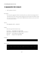
In this Manual, you will use GRASS 6.4.3. You can download it at
http://grass.osgeo.org/download.
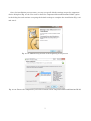
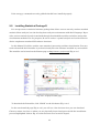
From the MS-Windows installer download page (Fig. 2-2-2), jump to the GRASS installer download page (Fig. 2-2-3) by clicking the “Free download of GRASS GIS for MS-Windows” link.
Fig. 2-2-1. GRASS home page
Fig. 2-2-2. GRASS download page
5
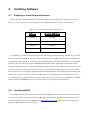
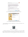
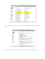
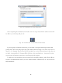
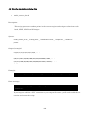
You can then download the GRASS installer for Windows by clicking the “WinGRASS-6.4.3-1Setup.exe” link in the download menu (Fig. 2-2-3).
Fig. 2-2-3. List of GRASS installers for various software versions
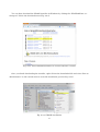
Once you finish downloading the installer, right click on the downloaded file and select “Run as
administrator” on the context menu to start the installation process (Fig. 2-2-4).
Fig. 2-2-4. GRASS installation
6
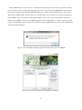
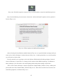
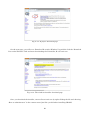
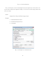
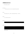
Once the installation process starts, you may accept all default settings except the component
choice dialog box (Fig. 2-2-6). You need to check the “Important Microsoft Runtime DLLS” option
in the dialog box and continue accepting the default settings to complete the installation (Fig. 2-2-7
and 2-2-8).
Fig. 2-2-5. GRASS setup wizard at the beginning of the process
Fig. 2-2-6. Choose the components you want to install (check “Important Microsoft Runtime DLLs)
7
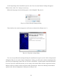
Fig. 2-2-7. Description of the Microsoft Runtime DLLs installation
Fig. 2-2-8. GRASS setup wizard at the end of the installation
If your installation is successful, the “GRASS GIS 6.4.3” icon (Fig. 2-2-9) will appear on your
desktop as shown below.
Fig. 2-2-9. GRASS startup icon
In addition to the desktop icon, you will see several GRASS short-cut icons under the GRASS
folder accessible from the Windows Start menu (Fig. 2-2-10). Each short-cut enables you to start
GRASS in a different mode such as a text mode or graphical user interface (GUI) mode. Later, we
8
will discuss how to use “GRASS GIS 6.4.3 GUI with MSYS” for data processing, so please remember how to find the short-cut icons.
To verify GRASS installed successfully, you may want to try starting GRASS in the “GRASS
GIS 6.4.3 GUI with MSYS” mode, as shown in Fig. 2-2-10.
Fig. 2-2-10. Various GRASS start modes in the program menu
After you select the “GRASS GIS 6.4.3 GUI with MSYS” start mode option, you will see a command window asking you to continue the GRASS startup process (Fig. 2-2-11).
Fig. 2-2-11. A command line window appears after you start GRASS GIS 6.4.3 in the MSYS
mode
9
Before GRASS starts, you may see a warning message (Fig. 2-2-12); however, ignore it and hit
the “ok” button. This warning message shows up when you start for the GRASS first time because
you haven’t assigned your default GRASS database yet. After you start GRASS, you will see the
“Welcome to GRASS GIS” window (Fig. 2-2-13) that allows you to choose a location and mapset to
start GRASS with. The purpose of starting GRASS is just to see if your installation completed
without any problems. So, close the GRASS application by clicking the “x” button on the top right
corner of the MSYS window. If you have problems starting GRASS, please refer to the FAQ section
at the end of this Manual.
Fig. 2-2-12. A warning message appears the first time you start GRASS
Fig. 2-2-13. Startup dialog box for GRASS with MSYS
10
2-3.
Installing OSGeo4W
OSGeo4W enables you to collectively install the latest open source GIS software and development libraries. You can avoid installing multiple copies of same libraries such as GDAL and Python on your machine if you use the OSGeo4W installation mechanism. Without this software, it is
common to have several software versions of, for example, Python, if you use standalone installers
to download GIS programs. OSGeo4W provides an effective way to manage your software and development environment related to geospatial data analysis. The official OSGeo4W website is
http://trac.osgeo.org/osgeo4w/.
Fig. 2-3-1. OSGeo4W project home page
The section “Quick Start for OSGeo4W Users” on the OSGeo4W home page (Fig 2-3-1) explains
how to install OSGeo4W and you simply need to follow the directions provided. First, click the
“OSGeo4W Installer” link to download the installer (osgeo4w-setup-x86_64.exe). Once you download the installer, run the installer “osgeo4w-setup-x86_64.exe” to start the installation process
(Fig. 2-3-2).
11
Fig. 2-3-2. Click the osgeo4w-setup.exe icon you downloaded to start the installation process
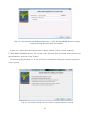
Once the installation processes starts, choose the “Advanced Install” option to select specific libraries (Fig. 2-3-3).
Fig. 2-3-3. Three options for OSGeo4W installation
After selecting the installation method shown in Fig. 2-3-3, accept the default settings until you
reach to the “Select Packages” window shown in Fig. 2-3-4. At that point there are several options
you will need to choose from.
For this tutorial, you are going to select the Python, GDAL and wxPython packages. (Amendment on February 1, 2015: Due to a change of the content of the OSGeo4 package, in addition to
these packages, you will need to also install gdal-python and python-numpy under Libs.)
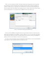
First, at the “Select Packages” wizard, expand the “Commandline_Utilities” list by clicking the
plus mark next to the Commandline_Utilities (Fig. 2-3-4). This will reveal the list of various command line programs, as shown in Fig. 2-3-5.
12
Fig. 2-3-4. A package selection wizard during OSGeo4W installation
Once you expand the “Commandline_Utilities” list, click “gdal” and “python-core” from the list
(Fig. 2-3-5). You may see different versions of gdal and Python compared with Fig. 2-3-5 since
OSGeo4W may have updated the available version after this Manual was published. Once you
chose gdal and python-core, then click the “Libs” list to select wxpython (Fig. 2-3-6).
13
Fig. 2-3-5. An expanded command line utility list during OSGeo4W installation
Fig. 2-3-6. Expanding the “Libs” category to select wxpython
Scroll down the expanded list and find wxpython from the list (Fig. 2-3-7).
14
Fig. 2-3-7. Selecting wxpython in the Libs category
After you select the wxpython package in the package list (Fig. 2-3-7), proceed and finish the installation process. It may take several minutes to complete the OSGeo4W installation process. Upon your successful installation, you will see the “OSGeo4W Shell” icon on your desktop.
2-4.
Installing pyModis
pyModis is a Python library used to download MODIS data from NASA’s FTP server. pyModis’s
official website is http://pymodis.fem-environment.eu/ (Fig. 2-4-1).
To install the pyModis program, click the “How to install pyModis” hyperlink on the pyModis
homepage (Fig. 2-4-1).
15
Fig. 2-4-1. pyModis’ home page
The pyModis library is managed by a source code management system called “git.” In order to
access the pyModis repository site, click the “github repository” hyperlink shown in Fig. 2-4-2 within the red circle.
Fig. 2-4-2. The red circle shows the hyperlink to the pyModis repository
16
If you have already installed “git client” you can access the pyModis source code using the “git
clone” command. Otherwise, click the “Download ZIP” button (Fig. 2-4-3) and download the source
code as a zip file.
Fig. 2-4-3. Github repository site for pyModis
After downloading the source code zip file, you will need to unzip the files. Find the setpu.py in
the unzipped files and execute setup.py script to install pyModis. To run the setup.py, you can use
the OSGeo4W Shell you already installed. Double click the OSGeo4W icon on your desktop to start
a command line. Then, move your current directory to the unzipped pyModis program directory.
Next, you can type the following command to start installing pyModis.
> python setup.py install
Notes: Once you add a path to the python.exe in the PATH setting, you can then use a
standard command line console (cmd.exe) to execute setup.py. The OSGeo4W Shell
makes this easy because it automatically sets up a path to python.exe, allowing you to
easily run setup.py.
17
If the setup.py command succeeds, pyModis should have installed properly.
2-5.
Installing Statistical Package R
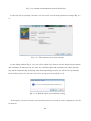
R is an open source statistical software package that allows users to not only conduct standard
statistical data analysis, but also develop data analysis environments with the R language. R provides various statistical analysis methods through downloadable modules and offers strong data
visualization methods. For our purposes, R can be used as a spatial analysis tool and its functionalities complement standard GIS software functions.
In this Manual, R will be used for some statistical processing and data visualization. You may
need to download the R installer if you don’t already have the software installed in your machine.
The installer can be found on the R home page at http://www.r-project.org/ (Fig. 2-5-1).
Fig. 2-5-1. R project home page
To download the R installer, click “CRAN” on the left frame (Fig. 2-5-1).
In the next download page (Fig. 2-5-2), you will see a list of mirror sites you can download.
Choose a mirror site close to where you are physically located and proceed with the installation
process (highlighted links in Fig. 2-5-2 show mirror sites located in Japan).
18
Fig. 2-5-2. R project download page highlighting mirror sites in Japan
On the next installation page (Fig. 2-5-3), select the download link that matches your operating
system.
Fig. 2-5-3. Choose an R installer based on your operating system
On the next page (Fig. 2-5-4), click the “base” hyperlink to continue the download process.
19
Fig. 2-5-4. R project download page
On the next page, you will see a “Download R 3.0.2 for Windows” hyperlink: click the “Download
R 3.0.2 for Windows” link and start downloading the R installer, R-3.0.2-win.exe.
Fig. 2-5-5. The windows installer download page
Once you download the installer, execute R-3.0.2-win.exe by right-clicking the file and choosing
“Run as administrator” in the context menu (just like you did when installing GRASS).
20
At the beginning of the installation process, the “User Account Control” dialog will appear.
When it does, click “Yes” and go to next step.
When the language selection dialog opens, select “English” (Fig. 2-5-6).
Fig. 2-5-6. Select Setup Language dialog
Then, finally, the actual setup process will start as shown below (Figure 2-5-7).
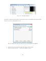
Fig. 2-5-7. R project setup dialog
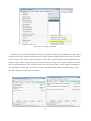
You can accept all default settings during the installation except for at the “Select Components”
dialog box (Fig. 2-5-8). At the “Select Components” dialog, you will need to choose installation files
based on your operating system (You can run the “32-bit Files” on both 32-bit and 64-bit Windows.
If you are not sure which OS version you are using, select 32-bit Files. All the scripts used in this
Manual will run on both a 32-bit and a 64-bit R environment.). Select the “Message translations”
option in the “Select Components” dialog box too (Fig. 2-5-8).
21
Fig. 2-5-8. Dialog for selecting components
After completing the installation, the R i386 3.0.2 icon (if you installed the 32-bit version) will
be added to your desktop (Fig. 2-5-9).
Fig. 2-5-9. R shortcut icon (32-bit R version shown)
If you use proxy for Internet connection, you will need to set up the following to install an R
package after this. Select the property by right clicking the R icon (Fig. 2-5-9), then your screen is
shown as "C:\Program Files\R\R-3.0.2\bin\x64\Rgui.exe" as the link destination in the short cut
tab. Add --internet2 like "C:\Program Files\R\R-3.0.2\bin\x64\Rgui.exe" --internet2. If you do
not use proxy for Internet connection, you will not need this setting.
To make sure your installation was successful and to install R packages, right click the R icon
to run as an administrator.start. If you see a similar window as shown in Fig. 2-5-10, you successfully installed R.
22
Fig. 2-5-10. R startup dialog
Once you have R working correctly, next you need to install spatial data analysis packages such
as sp and rgdal. To install these two R packages, you will need to execute the following “install.packages” statements. In the install.packages command, specify your install destination for
both packages. In this case, you want to specify the R library folder in the C:/Program Files/R/R3.0.2/.
> install.packages("sp", lib="C:/Program Files/R/R-3.0.2/library")
> install.packages("rgdal", lib="C:/Program Files/R/R3.0.2/library")
After you execute the first command, you may be asked to specify a download mirror site
(CRAN mirror). If so, you should be given the option to choose the closest mirror site from a list of
locations. You can also simply choose the first mirror site, “0-Cloud” as a generic mirror site.
23
Fig.2-5-11.Selecting a mirror site to download R packages
24
3.
Pre-processing Satellite Images
This chapter introduces the procedures required to download MODIS data and import those data into GRASS. This is the first step to create land cover type and tree cover maps. This chapter
also explains how to download and pre-process LANDSAT and VIIRS images. Once you have
downloaded MODIS images, you will learn how to create a land cover type map and a tree cover
map in chapters 4 and 5, respectively. To begin, however, you will execute a series of image processing commands provided as shell scripts. But even before you start processing images, you need
to set up your analysis environment and download MODIS images.
3-1.
Setting up the GRASS Environment
Before starting GRASS, first create a “C:\GIS_DATA\GRASS” directory to store all your
GRASS data. A default storage directory (for example, grass_data) may have been created during
the installation. We will use the “C:\GIS_DATA\GRASS” directory throughout this exercise.
You will execute all scripts through the MSYS console that starts automatically when you start
“GRASS GIS 6.4.3 GUI with MSYS.” So, if you haven’t started “GRASS GIS 6.4.3 GUI with MSYS,”
launch it now (Fig. 3-1-1).
Fig. 3-1-1. GRASS GIS 6.4.3 GUI with MSYS
After GRASS starts normally, the “Welcome to GRASS GIS” dialog shown in Figure 3-1-2 will
appear. You need to specify your data directory (recall, we are using C:\GIS_DATA\GRASS for
this exercise) by clicking the “Browse” button next to the “GIS Data Directory” text box. Once you
25
set your “GIS Data Directory,” your directory path will be shown in the text box (Fig. 3-1-2). If you
use an external hard disk to secure enough free disk space, create a new GRASS data directory
and specify the directory in the “GIS Data Directory” column.
Fig. 3-1-2. GRASS startup screen
In the next step, you will set up your GRASS location and mapset using the “Location wizard.”
You can access the location wizard by clicking the “Location wizard” button on the “Welcome to
GRASS GIS” dialog (Fig. 3-1-2).
With the Location wizard (Fig. 3-1-4) you can create a location interactively. First, enter the
GRASS Database Directory where a location will be created. For example, if you were using the
same directory path we designated, you would type “C:\GIS_DATA\GRASS” in the GRASS Data
Directory text box or select the target directory using a file chooser selected through the “browse”
button (Fig. 3-1-3). Next, enter a location name in the “Project Location” text box. We will use “Japan_LatLon” as a location name for this exercise (Fig. 3-1-3).
26
Fig. 3-1-3. Location wizard (GIS Data Directory: c:\GIS_DATA\GRASS; Project Location:
Japan_LatLong; Location Title: leave blank)
Figure 3-1-3 shows how the location named “Japan_LatLon” will be created under the
C:\GIS_DATA\GRASS directory. You can leave the “Location Title” box blank. Once you enter all
the information, press the “Next” button.
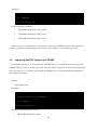
In the next dialog box (Fig. 3-1-4), you will select a method for setting the location’s spatial reference system.
Fig. 3-1-4. Location wizard screen to choose a spatial reference system
27
There are several methods available, including manually specifying spatial reference parameters, borrowing a reference definition from existing georeferenced data, and other methods. For
purposes of this exercise, we will define our spatial reference system by selecting an EPSG code.
Select the option titled “Select EPSG code of spatial reference system” and press the “Next” button.
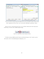
In the next dialog box, we are going to select an EPSG code from a list (Fig. 3-1-5).
Fig. 3-1-5. Location wizard to specify EPSG code
Since we will use WGS84 as our spatial reference system for data analysis, you need to specify
4326, which is the EPSG code for WGS84. As shown in Figure 3-1-5, you can type the code number
in the search box and then select the row listing 4326 in the selection box. After you highlight the
4326 row, click the “Next” button to continue the setup process.
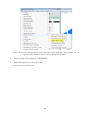
You may encounter the “Select datum transformation” dialog box (Fig. 3-1-6). Accept the default
setting (option 1) and click OK to finish the installation process.
28
Fig. 3-1-6. Datum transformation selection dialog box
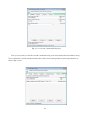
In the last step of creating a location, you can review your location parameter settings (Fig. 3-17).
Fig. 3-1-7. The summary of location settings
In the dialog window (Fig. 3-1-8), you will be asked if you want to set the default region extents
and resolution. In this exercise, we won’t set a default region and resolution since those parameters will be automatically set during other data importing processes you will need to go through
later in this exercise. So, for now, select “No” and go to next step (Fig. 3-1-8).
Fig. 3-1-8. Default region and resolution setting
At this point, you have created a new location and are now ready to create a mapset for your data analysis.
29
When creating a location, the software automatically creates a mapset named “PERMANENT.”
However, the PERMANENT mapset is a special mapset that should be used to store original data
intact, so it is a good practice to create a new mapset for use during your analysis. To facilitate
this process a “Create new mapset” wizard will automatically appear after you create a location, so
you simply need to type in the name of your new mapset. For purposes of this exercise enter the
mapset name “MODIS” and click the “OK” button (Fig. 3-1-9). These actions will create a mapset
named “MODIS.”
Fig. 3-1-9. Create a new mapset
If you create a mapset correctly, it will appear in the column titled “Accessible mapsets” (Fig. 31-10). You can now start GRASS by selecting a location (for this exercise select Japan_LatLon) and
a mapset (MODIS) from the lists, and clicking the “Start GRASS” button at the bottom of the wizard (Fig. 3-1-10).
30
Fig. 3-1-10. A newly created mapset is shown in the “Welcome to GRASS GIS” window
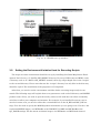
GRASS with the MYSIS mode starts with three windows (Fig. 3-1-11): GRASS GIS Layer Manager, GIS Map Display, and MSYS screen. The GRASS GIS Layer Manager (top left in Figure 3-111) is used to manage layers and enter various GRASS commands. The GIS Map Display (top
right) displays GRASS data. The MSYS screen (bottom) allows users to write out commands. We
will mainly use the MSYS window to type commands throughout this exercise.
31
Fig. 3-1-11. GRASS start-up windows
3-2.
Setting the Environment Variables Used for Executing Scripts
The script execution environment should be set up by installing the Global Map Raster Development Tool. Create a “C:\DATA\GSI_MODIS” directory (if you use USB connected HDD, create
a directory such as “F:\DATA\GSI_MODIS” instead), then copy all packaged files in the “/scripts”
to the created directory. Please note that not the “/scripts” directory but only files in the directory
should be copied. The installation of the programs is all completed.
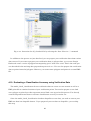
After that, you need to set the environment variables before executing image analysis commands. The following steps will explain how to set parameters such as the R directory and MODIS
product names. First, you need to open the modis_setenv.txt file with the text editor and modify
each line to reflect your computer environment. For example, if you installed R version 3.0.3 instead of version 3.0.2, you need to reflect the version difference in the R_BIN and RSC_BIN settings. You also need to specify the MODIS product information you are going to use. For the 1 km
resolution MODIS images, use MCD43B4 as the PRODUCT_NAME and MCD43B2 as the
QC_NAME settings. For the 500 m resolution images, use MCD43A4 and MCD43A2 instead.
32

OSGeo4W_PATH
:OSGeo4W install path (e.g. "/c/OSGeo4W")

R_BIN
:R.exe full path (e.g. "/c/Progra~1/R/R-3.0.2/bin/x64/R.exe")

RSC_BIN
:Rscript.exe full path (e.g. "/c/Progra~1/R/R-3.0.2/bin/x64/Rscript.exe")

R_LIBS
:R library full path (e.g. "/c/Progra~1/R/R-3.0.2/library")

PRODUCT_NAME
: MODIS product name (e.g. MCD43B4 or MCD43A4)

QC_NAME
: MODIS QC product name (e.g. MCD43B2 or MCD43A2)

COLLECTION
: MODIS product collection number (e.g. 005)
Notes: Scripts may not work properly if you include a space in the path. To avoid problems
later, please make sure to specify an alias name that doesn’t include spaces. You can confirm each path’s alias using the “dir /x” command (e.g., “Progra~1” is set as an alias for
“Program Files”).
Notes: You also need to set the R_LIBS variable. A path to the R library depends on where
you install R packages in Section 2-5. If you follow the steps in 2-5 exactly, you should set a
full path the same as explained above. If you did not start R as an administrator, your library path may be in the user folder instead (e.g. c:\users\yourname\Documents\R\winlibrary\3.0).
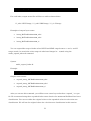
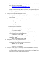
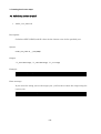
Fig. 3-2-1. An example of modis_setenv.txt (You may need to modify the highlighted lines)
You don’t need to change environment variables in the modis_setenv.txt except for the above
seven settings. When you finish editing the file, you need to update and confirm the environment
settings manually by running the following command. This process is recommended even if you
didn’t change the modis_setenv.txt.file.
33
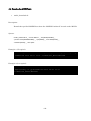
> cd /c/DATA/GSI_MODIS
> source modis_setenv.txt
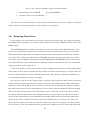
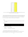
You can check whether your analysis environment is updated with the modis_printenv.sh script.
This script returns the environment variables you set in the modis_setenv.txt. Once you confirm
your variable settings, you don’t need to run the “source” command again so long as you keep
working through this tutorial and keep GRASS open and active. However, if you close the GRASS
and MSYS console, you will need to run the “source” command again to load the variable settings.
Each script you will use in the following steps includes a function to load the environment settings
if the variables are not set. However, this mechanism only works if a target script is in the same
directory as the modis_setenv.txt.
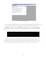
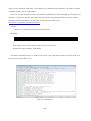
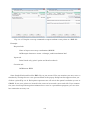
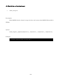
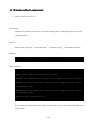
>sh modis_printenv.sh
--- parameter values --OSGEO4W_PATH=/c/OSGeo4W
R_BIN=/c/Progra~1/R/R-3.0.2/bin/x64/R.exe
RSC_BIN=/c/Progra~1/R/R-3.0.2/bin/x64/Rscript.exe
PRODUCT_NAME=MCD43B4
QC_NAME=MCD43B2
COLLECTION=005
PATH=/c/OSGeo4W/bin:/C/Program Files (x86)/GRASS GIS 6.4.3/lib: …
PYTHONHOME=/c/OSGeo4W/apps/Python27
GDAL_DATA=/c/OSGeo4W/share/gdal
MODIS_DOWNLOAD_PY=/c/OSGeo4W/apps/Python27/Scripts/modis_download.
py
3-3.
Downloading MODIS Data
MODIS is a visible and infrared radiometer onboard NASA's TERRA and AQUA observation
satellites. MODIS’s spatial resolutions are between 250 and 1000 m. These spatial resolutions are
lower than other medium/high resolution sensors; however, MODIS can capture 36 spectral bands
and record images at a high temporal frequency. In fact, MODIS acquires an image of the same
area once or twice a day. TERRA passes through the equator in the morning, and AQUA passes
34
through the equator in the afternoon. This technology thus allows you to obtain various types of
data such as land cover, vegetation, forest fires, land surface reflectance, and ocean surface temperature. “Land Products,” which is a MODIS product series, is created, distributed, and stored by
the Land Processes Distributed Archive Center (LP DAAC) (Fig. 3-3-1).
For more information about MODIS, please check following website:
https://lpdaac.usgs.gov/products/modis_overview.
Fig. 3-3-1. LP DAAC home page (https://lpdaac.usgs.gov/)
The LP DAAC creates and distributes various MODIS products. We will use MCD43B4 and
MCD43B2 for our exercise. MCD43B4 is a 16-day composite, 1 km resolution, 7-band data product
synthesized with TERRA and AQUA images, whereas MCD43B2 is a product designed for data
quality assurance and quality control (“QA/QC”). If you want to analyze the 500 m resolution images instead, use MCD43A4 and MCD43A2 products.
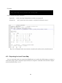
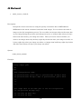
To download MODIS products, use modis_download.sh. Before executing the command, it is a
good idea to create a data folder to store downloaded data. From here to Section 3-5 of this Manual,
we will use MCD43B4 to describe how to download data and complete other processes. After you
complete this initial process, you can conduct same processes by simply replacing MCD43B4 with
MCD43B2.
35
> mkdir /c/DATA/GSI_MODIS/MCD43B4
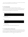
The modis_download.sh script downloads specific MODIS products for a given time period and
spatial extent. The modis_download.sh will automatically download data for the same date range
you set for the previous and the following year. For example, if you download images between
2012/09/01 and 2012/10/31, modis_download.sh automatically downloads images taken between
2011/09/01 and 2011/10/31 as well as images between 2013/09/01 and 2013/10/31.
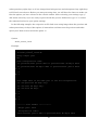
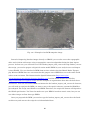
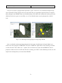
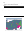
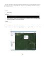
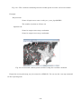
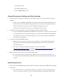
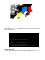
You can download several image tiles by specifying MODIS’s tile numbers in the
modis_download.sh command. The LP DAAC stores images as tiles and each tile has horizontal (h)
and vertical (v) numbers. For example, h28v04, h28v05, and h29v05 tiles almost entirely cover the
Japanese archipelago (Fig. 3-2-2).
Fig. 3-2-2. The MODIS tile system viewed with Google Earth
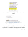
You can use a KML file freely available for download from Oak Ridge National Laboratory Distributed Active Archive Center (ORNL DAAC) to check MODIS tile numbers. You can find the
KML file download link at http://daac.ornl.gov/MODIS/ (Fig. 3-2-3).
36
Fig. 3-3-3. The MODIS sinusoidal GRID KML download link at the ORNL DAAC home page
modis_download.sh accepts the following arguments.
Syntax:
modis_download.sh –t [tile number(s)] –r [xmin, ymin, xmax, ymax] [e-mail address]
[tile] [product name] [year] [start date] [end date] [save path]
Notes:
•
You cannot use the –t and –r options at the same time.
•
You can download multiple tiles in one process by specifying tile numbers using a comma as a separator.
•
You can specify the spatial extent of images you download by the –r option
with the 4 boundary coordination. You need to specify latitude and longitude
as decimal degrees.
37
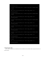
The following statement downloads MCD43B4.005 products that cover all of Japan (tile codes of
h28v04, h28v05, and h29v05) between September 1 and October 31, 2012.
Example 1 (tile option):
> sh modis_download.sh
-t h28v04,h28v05,h29v05
[email protected] MCD43B4.005 2012 09-01 10-31
/c/DATA/GSI_MODIS/MCD43B4
Download file name examples:

MCD43B4.A2011249.h28v04.005.2011266182944.hdf

MCD43B4.A2011249.h28v05.005.2011266184219.hdf

MCD43B4.A2011249.h29v05.005.2011266184810.hdf
Example 2 (range option):
> sh modis_download.sh -r 138.5 35.2 140.5 36.7
[email protected] MCD43B4.005 2012 09-01 10-31
/C/DATA/GSI_MODIS/MCD43B4
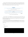
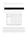
After running the above command, the image download process will start and specified MODIS
products will be stored in the directory you originally identified (Fig. 3-3-2). You may encounter a
python error during the download process. In spite of this error message sometimes created by
pyMoids, you can still continue to download images.
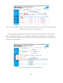
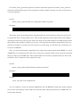
Next, download MCD43B2 products and store the downloaded files to the same directory you
used for MCD43B4 files. The sequence of analysis requires that you store a pair of MODIS products (e.g. MCD43B4 and MCD43B2) in the same directory. If you want to use the MODIS 500 m
products, you need to make a different directory and store the image and QA/QC products in the
same directory such as MCD43A4 (/C/DATA/GSI_MODIS/MCD43A4).
Example 1 (downloading QA/QC products in the MCD43B4 directory):
> sh modis_download.sh -t h28v04,h28v05,h29v05 [email protected]
MCD43B2.005 2012 09-01 10-31 /C/DATA/GSI_MODIS/MCD43B4
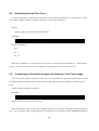
38
Fig. 3-3-2. Downloaded MODIS image files
3-4.
Reprojecting and Merging Images
Downloaded MODIS data adopt the Sinusoidal projection system and the HDF file format. You
will often use several image tiles to cover your areas of interest. Therefore, you need to merge and
reproject your images for the image analysis. Additionally, you will need to separate bands into
single band images for later processes. We will use the modis_merge.sh script for these processes.
To reproject, merge, and separate images, you need to first copy the modis_merge.sh script to
your working directory, MCD43B4. Since modis_merge.sh removes all directories under the current directory, you need to make sure that you run this script only in a working directory such as
MCD43B4. We also recommend checking if the product settings in the modis_setenv.txt match the
downloaded files (in this case MCD43B4 and MCD43B2 files) in the directory. In the data directory
you should only have data you specified in the modis_setenv.txt.
As this software may have an unexpected behavior with regard to the extent of merging the image, we recommend you to enter xmin, ymin, xmax, and ymax.
Syntax:
modis_merge.sh [(optional) xmin␣ymin␣xmax␣ymax]
39
Example:
> cp modis_merge.sh ./MCD43B4
> cd ./MCD43B4
> sh modis_merge.sh
Output filename examples:

MCD43B4.A2012249_band1_prj.tif

MCD43B4.A2012249_band2_prj.tif

MCD43B4.A2012249_band3_prj.tif
After the process is completed, you will have a series of GeoTIFF files that hold reprojected,
merged, and band separated image data for the series of dates you originally specified.
3-5.
Importing GeoTIFF Images into GRASS
In the following step, you will import the GeoTIFF files you created in the last process into
GRASS GIS. You will use modis_import.sh to do this. modis_import.sh should be executed in the
directory where you previously downloaded the MODIS data. Type the following commands to
start importing images.
Syntax:
modis_import.sh
Example:
> cd /c/DATA/GSI_MODIS
> cp modis_import.sh ./MCD43B4
> cd ./MCD43B4
> sh modis_import.sh
Examples of imported layer names:

MCD43B4.A2012249_band1
40

MCD43B4.A2012249_band2

MCD43B4.A2012249_band3
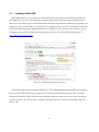
By executing modis_import.sh, MODIS data is automatically imported into GRASS. Layer
names of those imported images are assigned based on the original TIFF file names. GRASS automatically sets its region setting based on the range of images you will import and determines its
spatial resolution setting based on the first imported image.
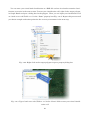
You can display imported single band images by clicking the “Add raster map layer” menu in
the GRASS toolbar. You are also able to display a RGB composite image with three band images
by clicking “Add various raster map layers” in the GRASS toolbar and choosing the “Add RGB map
layer” command. However, maps you wanted to see may not have suitable color settings. In that
case, you need to assign a different color map to each layer by using the r.colors command (Fig. 35-1). We recommend you choose the “gray255” color map with the “Histogram equalization” option
(Fig. 3-5-2).
Fig. 3-5-1. Using the r.colors command in GRASS to change a map’s color setting
41
Fig. 3-5-2. Choose a target map in the “Required” tab, select “gray255” from the “Type of color
table” dropdown list in the “Colors” tab, and check the “Histogram equalization” option
After you set up a color map for each layer, you can click the “Add various raster map layers”
button (Fig. 3-5-3) and create a RGB composite image.
Fig. 3-5-3. Add various raster map layers menu
To finish creating the RGB composite image, specify band1 image as “red,” band4 as “green,”
and band3 as “blue” in the RGB composite dialog (Fig. 3-5-4).
42
Fig. 3-5-4. RGB composite image dialog
A composite RGB image may look like Figure 3-5-5.
Fig. 3-5-5. RGB composition image (R: band1, G: band4, B: band3)
Again, if you want to use the MODIS 500 m products (MCD43A4 and MCD43A2), you need to
repeat the same procedures described in sections 3-2 to 3-5, replacing “MCD43B4” with “MCD43A4”
for each image processing command. Don’t forget to change the modis_setenv.txt settings.
43
3-6.
Managing Intermediate Data
You are about to start a series of image processing using GRASS. During the processes, you will
create lots of intermediate data and you may want to delete those files at some point. There is no
automated file management function in this program, so you must manually manage your map
data in GRASS. The most efficient way to delete multiple files is to use the g.mremove command.
This command allows you to filter maps using a wild card or a regular expression and delete them
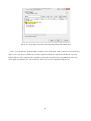
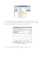
at once. For example, if you want to delete all maps that have “old_” at the beginning of the map
names, you can type “old_*” in the “rast file(s) to be removed” column in the g.mremove command
window (Fig. 3-6-1). You can find the g.mremove command in the File menu / Manage maps and
volumes / Delete filtered (g.mremove). You need to check the “Force removal (required for actual
deletion of files)” option for the actual file removal. Without this option, this command only returns
map names that match the condition you specified. The g.remove command is also the best tool to
delete single or multiple maps that are difficult to select by a wild card or regular expression.
Fig. 3-6-1. g.mremove command for a multiple map deletion
It is often convenient if you can overwrite existing maps during your data analysis. GRASS provides the “Allow output files to overwrite existing files” option for many commands. If a command
44
has this option, you can reduce intermediate maps when you want to repeat the same analysis
with different parameter settings. If a command or script does not allow you to overwrite existing
maps, you need to be sure to change output map names to avoid runtime errors.
3-7.
Limiting Analysis Extent with a Mask
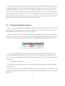
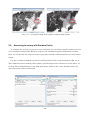
You can limit your analysis extent using a mask layer. A masking technique not only makes
your process more efficient, but it also makes your process faster. You can easily create your own
mask from existing GIS data from the Global Map project. We will download the political boundary
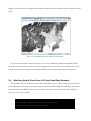
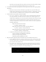
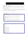
area data (vector data) and create a mask to include only the land portion of Japan (Fig. 3-7-1).
Fig. 3-7-1. Before (left) and after (right) applying a mask
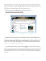
You can download the political boundary area data for various countries from the International
Steering Committee for Global Mapping’s (ISCGM) website (http://www.iscgm.org/). For Japanese
boundary data, you can visit http://www.gsi.go.jp/kankyochiri/globalmap_e.html and follow the
link “Download Global Map Japan.” (Fig. 3-7-2).
45
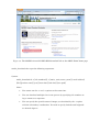
Fig. 3-7-1. Global Map Japan download page
(http://www.gsi.go.jp/kankyochiri/globalmap_e.html)
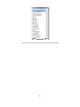
Fig. 3-7-2. Downloadable data list at the Global Map Japan site (red circle: the political boundary data)
Once you reach the download site, download a political boundary shapefile to your destination
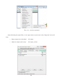
directory and import the files into GRASS. You can use v.in.ogr command (Fig. 3-7-3) for this purpose.
46
Fig. 3-7-3. v.in.ogr command to import vector data into GRASS
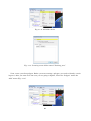
Once you select the v.in.org command from the file menu (Fig. 3-7-3), select the downloaded political boundary data as a source file and run the command (Fig. 3-7-4).
Fig. 3-7-4. v.in.ogr dialog box to import vector data (settings are described below)
•
Format:
Shapefile
•
File:
source shapefile
•
Layer name:
polbnda_jpn
•
Name for GRASS map:
polbnda_jpn
47
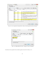
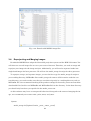
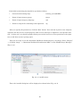
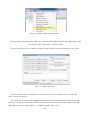
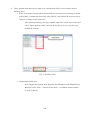
The imported political boundary data are composed of prefecture boundary polygons (Fig. 3-75). Therefore, you need to dissolve the polygons to create a unified Japanese political boundary.
Fig. 3-7-5. Political boundary polygons and their attribute table (the yellow highlighted coc
field holds a common attribute across all polygons)
To dissolve the boundaries, use the v.dissolve command and a field that contains a common attribute across the all polygons: in this case, use the “coc” field in the boundary data. You can find
the v.dissolve command under the vector menu (Fig. 3-7-6).
48
Fig. 3-7-6. v.dissolve command under the Vector menu
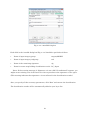
Once the v.dissolve command dialog box appears, you can specify parameters as follows (Fig. 37-7):
Required tab
•
Name of input vector map:
polbnda_jpn@MODIS
•
Name for output vector map: jpn_msk
Optional tab
•
Name of column used to dissolve common boundaries:
coc
Fig. 3-7-7. v.dissolve dialog box
After you conduct the v.dissolve command, you will have one polygon that represents the land
part of Japan. In the next step, convert the dissolved polygon into the GRASS raster format using
v.to.rast command (Fig. 3-7-8). You will use this rasterized polygon to create a mask.
49
Fig. 3-7-8. v.to.rast command will convert an input vector map into raster format. You can
specify each parameter in the v.to.rast dialog box as below.
•
Name of input vector map: jpn_msk@MODIS
•
Name for output raster map: jpn_mask
•
Source of raster values: cat
50
Fig.3.7-9. v.to.rast command dialog box
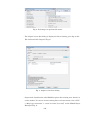
Now you are ready to run the r.mask command using your rasterized political boundary map.
You can find the r.mask command under the raster menu and specified required parameters as
below (Fig 3-7-10).
51
Fig. 3-7-10. r.mask command to apply an analysis mask
•
Raster map to use as MASK:
jpn_mask@MODIS
•
Category values to use for MASK:
*
You also can use this technique to create a mask with a different area, for example a small part
of the country, instead of treating the entire country as one polygon.
3-8.
Removing Cloud Cover
In this section, you will learn how to use the cloud removal script. Since this script runs within
the GRASS GIS environment, you need to work on this tutorial in the “GRASS GIS 6.4.3 GUI with
MSYS” mode.
Most MCD43B products include some cloud-covered areas. Since clouds hide land cover, they
cause issues with image classification. To ameliorate image classification quality, we will extract
information from images taken in a different time period and use that data to fill in the clouded
area pixels. The quality assessment data, MCD43B2, will tell us the extent of cloud cover. Therefore, make sure you download and preprocess both MCD43B2 and MCD43B4 products before you
start the following exercise. Additionally, to limit the analysis to land (not water), we recommend
setting a mask as we described in 3-7.
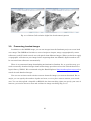
To fill in the cloud-covered areas, we will evaluate weighted average raster values using images
taken either 48 days before and after the date image was taken (total 96 days), or images taken on
the same date during the previous and subsequent years. This process is little bit complicated, so
we will explain this process using an example.
Let’s say you want to run the modis_remove_cloud.sh script for the year 2012. Once you run the
modis_remove_cloud.sh, type “2012” to specify your target year and hit return. This command is
interactive and so the program will next ask you in what order it should choose images for filling
the cloud-covered areas (search order option). You can choose from two methods. The first method
will use images from the previous and subsequent years to fill cloud-covered areas first, and use
the images taken in the previous and subsequent ninety-six days if there are still cloud-covered
areas. On the other hand, the second method uses images taken in the previous and subsequent
ninety-six days first, and then uses the previous and subsequent years’ images next. After you
choose the first option, select the next option to choose the data you are going to use (data option).
You can chose (1) use only images from the previous forty-eight days; (2) use only images from the
52
subsequent forty-eight days; or (3) use images from both previous and subsequent forty-eight days
to fill cloud-covered areas. Before you start processing data, you will have the chance to make confirm the options you have selected in the console window. After reviewing your settings, type “y”
and hit the enter key if you are ready to proceed with the process. Otherwise, type “n” to restart
the command and revise your option settings.
In the following example, the script tries to fill cloud areas using images from the previous and
subsequent ninety-six days (data option: 3) in 2012 first and then uses the previous and subsequent years’ data next (search order option: 1).
Syntax:
modis_remove_cloud
Example:
> cd /c/DATA/GSI_MODIS
> sh modis_remove_cloud.sh
Specify target year
2012
Choose interpolation order.
1): previous/next year's data => previous/next 96 day's data
2): previous/next 96 day's data => previous/next year's data
1) 1
2) 2
#? 1
1
Select image data of the same year to use for interpolation.
1): use previous 48 days only.
2): use next 48 days only.
3): use both 48 days.
1) 1
2) 2
3) 3
#? 3
3
---------- Your answer ------------ Target year: 2012
- Interpolation order:
previous/next year's data => previous/next 48 day's data
53
- Image data to use:
use both 48 days.
Now it's ready to process. Execute (y/n) ?
y
Examples of output layer names:
•
interp_MCD43B4.A2012249_band1
•
interp_MCD43B4.A2012249_band2
•
interp_MCD43B4.A2012249_band3
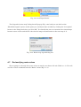
The modis_remove_cloud.sh process will create a series of GRASS raster data with a prefix of
“interp_”. This script is not sensitive to the current path you are in when you execute it because
this script deals with GRASS data.
Some pixels in the cloud-removed images may have null values. To remove these null values,
use modis_fillnull.sh. This script uses an inverse distance weighting (IDW) technique to fill null
values. This script will create a new, null-free set of raster data with the same name as its input
data. The original data will be renamed with the prefix “old_” during the process.
Syntax:
modis_fillnull.sh [target year]
Example:
> sh modis_fillnull.sh 2012
Examples of output layer names:
•
old_interp_MCD43B4.A2012249_band1
•
old_interp_MCD43B4.A2012249_band2
•
old_interp_MCD43B4.A2012249_band3
54
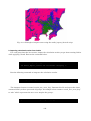
Fig. 3-8-1. Before (left) and after (right) the cloud removal process
3-9.
Processing Landsat images
In addition to the MODIS image, you can use images from the Landsat8 project to create land
cover maps. The GMRD tool includes a series of scripts to import, merge, topographically correct
reflectance, and fill cloud-covered area with pixels from different images. When you decide to apply
a topographic collection on your images before importing them into GRASS, digital numbers will
be converted into reflectance automatically.
There is no automated image downloading mechanism for Landsat. So, as your first step, you
need to manually download images from Landsat image providers such as the United States Geological Survey (USGS). We recommend using the Earth Explorer (http://earthexplorer.usgs.gov/) to
search for and download images.
You can use various search criteria to narrow down the images you want to download. For example, you can specify the number of paths and rows, or use a place name to narrow your search
area. You can also upload a shapefile or KML file for data searching. After you specify your area of
interest, you need to choose a start and end date for image searching (Fig. 3-9-1).
55
Fig. 3-9-1. USGS’s Earth Explorer home page
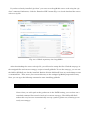
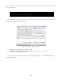
Next, you need to specify a data set to search. In our case, select “L8 OLI/TIRS” in the “Landsat Archive” list (Fig. 3-9-2). After you choose the data set option, search results will appear in the
“Result” tab. You can check the metadata of those images or their thumbnails to decide which images are useful for your analysis. Once you decide what image you want to download, click the
“download” button (Fig. 3-9-3) and start downloading the image.
Fig. 3-9-2. Options to select satellite image products using USGS’s EarthExplorer
56
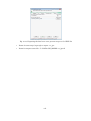
Fig. 3-9-3. A download link in the USGS’s EarthExplorer
When you click the download icon in Figure 3-9-3, the “Download Option” dialog box will appear and you should choose the “Level 1 Geo TIFF Data Product” option and proceed with the
download process. If you haven’t created your image download account on the EarthExplorer site,
you need to create one at this time.
Fig. 3-9-4. “Download Options” dialog box to choose a product to download
If you are ready to download data, you will see the “Download Scene” dialog box (Fig. 3-9-5).
You can click the “Download” button to start downloading the image.
57
Fig. 3-9-5. “Download Scene” dialog box in the USGS’s EarthExplorer
If you want to fill cloud-covered areas, you need images from forty-eight days before and after
your target date. Additionally, you may need to download more images if you need multiple Landsat images to cover your study area. Once you obtain the necessary series of images, you can automate image processing. You need to store all downloaded images into the same folder to automate the data import process. For this exercise, we are going to create a “landsat” folder under the
/DATA/GSI_MODIS directory.
Once you finish downloading images, you need to check the landsat_setenv.txt file to make
sure all environ parameters are correct to run scripts. The contents of the landsat_setenv.txt are
almost identical to modis_setenv.txt except for the product name setting (Fig. 3-9-6). You need to
set the PRODUCT_NAME parameter as LO8 (Fig. 3-9-6). Once you load the environmental settings using the “source” command in MYSIS, your environmental settings will be updated. If you
want to analyze MODIS data again, you need to load modis_setenv.txt again.
Fig. 3-9-6. Landsat_setenv.txt and its contents
A command to load the environment settings:
cd /c/DATA/GSI_MODIS
cp landsat_setenv.txt ./landsat
58
cd ./landsat
source landsat_setenv.txt
You will use the landsat_import.sh script to import Landsat images. First, you need to copy the
landsat_import.sh script to the directory where you stored the Landsat images. Then you can run
the script from that same directory. You can automatically import all images you stored in the
folder with this script.
Syntax:
Landsat_import.sh
Example:
cd /c/DATA/GSI_MODIS
cp landsat_import.sh ./landsat
cd ./landsat
sh landsat_import.sh
Once you import the Landsat images, you can load images in an RGB composite format using
the “Add RGB map layer” command. If you want to see the image in its natural color, you need to
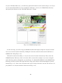
specify band 4 as red, band 3 as green, and band 2 as blue (Fig. 3-9-7).
59
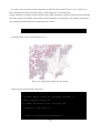
Fig. 3-9-7. Example of an RGB composite image
Instead of importing Landsat images directly to GRASS, you can also correct the topographic
effect and calculate reflectance using a topographic correction algorithm during the data import
process. In that case, you will need to use the landsat_import_and_correct.sh script. Before you run
that script, you need to prepare a digital elevation model (DEM) in your analysis area and import
it into GRASS. You can download a DEM from various websites but the Shuttle Rader Topography Mission (SRTM) data are convenient for this purpose since SRTM data cover the entire world
with a 90 m resolution. The Consortium for Spatial Information (http://www.cgiarcsi.org/data/srtm-90m-digital-elevation-database-v4-1) and the Global Land Cover Facility
(http://www.landcover.org/data/srtm/) are two examples of organizations that offer the data download service. You can use various DEM resolutions for the landsat_import_and_correct.sh; however,
you will need to reproject the DEM you want to use to the spatial reference system the GRASS region adopted. The script uses GDAL to read DEM. Therefore, the script’s file format will depend on
the GDAL specification. You’ll need to make sure your DEM is based on metric units, but you can
use either integer or float data type DEMs.
Once you prepared the DEM, you need to copy the landsat_import_and_correct.sh to the Landsat directory and execute the script for each downloaded data.
60
Syntax:
landsat_import.sh [input file (tar.gz)] [DEM layer]
Example:
> sh landsat_import_and_correct.sh LC81080352013283LGN00.tar.gz
dem_4326
Output files:
•
LC81080352013283LGN00_B1
•
LC81080352013283LGN00_B2
•
LC81080352013283LGN00_B3
Once you import images into GRASS, you can merge images that were taken on the same date
but different paths and rows.
Syntax:
landsat_apply_qc.sh
Example:
> sh landsat_apply_qc.sh
Finally, you can fill the cloud-covered pixels with images from another time period using the
same process we explained in Section 3-8. Before you run the landsat_intepolate.sh script, you
need to download Landsat images either from forty-eight days before and after the date the image
was taken (total ninety-six days), or from images taken on the same date during the previous and
subsequent years. The landsat_interpolate.sh script allows you to choose which of these methods
you prefer to fill in cloud-covered areas. In the landsat_interpolate.sh script, you need to first specify a target year, and then identify your preferred filling method. Refer to Section 3-8 for more specific information.
Syntax:
landsat_interpolate.sh
Example:
61
> sh landsat_interpolate.sh
3-10. Processing VIIRS images
VIIRS is another source of satellite images from which you can create land cover data. You can
download VIIRS images from the National Oceanic and Atmospheric Administration’s (NOAA)
website (http://www.nsof.class.noaa.gov/saa/products/search?datatype_family=VIIRS). For this exercise, we will assume you will download the Image Band EDR products (band 1 ~ 3) to run VIIRS
related scripts.
Similar to the Landsat processing, there is no automated image downloading mechanism for
VIIRS. So, as your first step, you need to manually download images from the image provider (Fig.
3.10.1).
Fig. 3-10-1. NOAA’s VIRRS image download site
To search for the images you want to download, you can set a time period as well as location as
search criteria (Fig. 3-10-2).
62
Fig. 3-10-2. Specify a time period and location for your image search
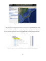
You also need to select a data product to download from the long list under the temporal search
section. For this exercise, scroll down the site and find the “Environmental Data Record” list and
select the “VIIRS Imagery Band 01 ~ 03 EDR” options (Fig. 3-10-3). Then you can click the “Search”
button and start the image search (Fig. 3-10-4). If it takes too long to get a search result, you may
have set your temporal search criterion too long or your spatial criterion too wide. In that case, you
may need to narrow your search criteria.
63
Fig. 3-10-3. Select VIIRS Imagery Band 01 ~ 03 EDR from the Environmental Data Record list
(highlighted)
Fig. 3-10-4. Click the “Search” button to start searching for images
After the image search finishes, a list of VIIRS images matching your criteria will show up (Fig.
3-10-5). You can check each image and decide which images you want to download. You need to
select the check boxes for each image (Fig. 3-10-5) and click the “Update” button to put the images
into your “Shopping Cart.” After you have selected all the images you want to download and updated the list one last time, you can click the “Goto Cart” button to move to the shopping cart page.
64
Fig. 3-10-5. An example of image lists ((1) Check the images you want to download; (2) Update the
selection list; and (3) Go to the shopping cart)
On the shopping cart page (Fig. 3-10-6), you will see the image list you chose. If you already
have an image download account, you will see the “Place Order” button; however, if you don’t yet
have an account, the “Register” button will appear instead (Fig. 3-10-6) and you can register with
your name and email address.
Fig. 3-10-6. An image list in the shopping cart
65
After you click the “Place Order” button, the site will take you to the “Confirmation” page of
your order (Fig. 3-10-7). You will see your order number and some information about the time it
takes for NOAA to prepare your data for download. You will receive an email message once your
order is ready to download (this typically takes several hours or longer).
Fig. 3-10-7. Order confirmation page
Once you obtain a series of VIIRS images, you can automate image processing just like we did
with Landsat images. Again, you will need to store all the downloaded images in the same folder to
automate the data import process. For this exercise, we are going to create a “viirs” folder under
the /DATA/GSI_MODIS directory.
You will use the viirs_import.sh script to import VIIRS images. First, you need to copy the
viirs_import.sh script to the directory where you stored the VIIRS images. Then, you can run the
script from the same directory. You can automatically import all images you stored in the folder
with this script.
Syntax:
viirs_import.sh
Example:
cd /c/DATA/GSI_MODIS
cp viirs_import.sh ./viirs
cd ./viirs
sh viirs_import.sh
66
You can only import the radiance data from the downloaded hdf5 data file. The viirs_import.sh
will not convert the original digital numbers (DN) during the importing process.
Once you have imported all VIIRS images into GRASS, you can run the viirs_merge.sh to
merge images for each band. This script merges images that were taken on same date but in different paths and rows. You need to include both band 1 and band 2 images in the imported data
since this script uses those bands to calculate NDVI to select the better quality pixels from images
that overlap each other.
Syntax:
viirs_merge.sh
Example:
> sh viirs_merge.sh
67
4.
Creating a Land Cover Map
In this chapter, we will develop a land cover (LC) map using a supervised classification (either a
maximum likelihood or a decision tree method) with the MOIDS images you imported in the last
chapter.
4-1.
Acquiring Training Data for Your Image Classification
If you don’t already have your own training data for use in creating a LC map, you can generate
training data using software, such as Google Earth. First, start Google Earth and zoom to an area
you are interested in.
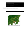
Fig. 4-4-1. Google Earth startup screen
Next, make a new folder to store all your training area polygons. To make a new folder, you
need to select “Folder” under the “Add” menu as shown in Fig. 4-1-2. You may name the folder
“training_area” (Fig. 4-1-3).
68
Fig. 4-1-2. Add folder menu
Fig. 4-1-3. Creating a new folder named “Training_area”
Next, create your first polygon. Before you start creating a polygon, you need to identify a training area. After you zoom in on the area you are going to digitize, select the “Polygon” under the
“Add” menu (Fig. 4-1-4).
69
Fig. 4-1-4. Add polygon menu
The “New Polygon” dialog box appears (Fig. 4-1-5). In the new polygon dialog box, you need to
input the land cover code you are interested in into the “Name” field (Fig. 4-1-5). We will use Table
4-1-1 as our LC code table for this exercise. You don’t need to add any other information in the dialog box.
Fig. 4-1-5. A new Polygon dialog box in Google Earth
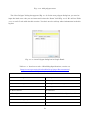
Table 4-1-1. Land cover code—Global Map Specifications, version 1.3
(http://www.iscgm.org/cgi-bin/fswiki/wiki.cgi?page=Documentation)
Current land cover
1. Broadleaf Evergreen Forest
11. Cropland
2. Broadleaf Deciduous Forest
12. Paddy field
3. Needleleaf Evergreen Forest
13. Cropland/Natural Vegetation Mosaic
4. Needleleaf Deciduous Forest
14. Mangrove
5. Mixed Forest
15. Wetland
6. Tree Open
16. Bare area, consolidated (gravel, rock)
7. Shrub
17. Bare area, unconsolidated (sand)
8. Herbaceous, single layer
18. Urban
9. Herbaceous with Sparse and Tree/Shrub
19. Snow/Ice
70
10. Sparse Vegetation
20. Water Bodies
Now you can draw a polygon that represents a “pure” land cover. You should encompass large
areas if possible. If the polygon areas are too small, they are sometimes ignored when you import
those polygons into GRASS. After you finish drawing, click “OK” and continue the same process for
different land cover types or areas (Fig. 4-1-6). You should obtain several polygons for each LC
type.
Fig. 4-1-6. Drawing training polygons using Google Earth
Once you finish creating training polygons for the image classification in Google Earth, you
need to save the polygons as KML files. To create a KML file, right click on the training_area folder and select the “Save Places As…” option. You can choose any name for the KML file, but for
purposes of this exercise we will name the file “training_area.kml”. In the following section, we will
import the training data you created into GRASS.
71
Fig. 4-1-7. Procedure for saving a KML file
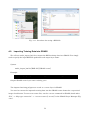
4-2.
Importing Training Data into GRASS
We will use modis_import_kml.sh to import the KML training data into GRASS. You simply
need to specify the input KML file path/name and output layer name.
Syntax:
modis_import_kml.sh [KML file] [GRASS vector]
Example:
> sh modis_import_kml.sh training_area.kml training_area
Output GRASS vector layer name: training_area
The imported training polygons are saved as a vector layer in GRASS.
You need to convert the imported training data into the GRASS raster format for a supervised
image classification. To convert to raster files, use the v.to.rast command in GRASS, found under
“File” --> “Map type conversion” --> “vector to raster [v.to.rast]” in the GRASS Layer Manager (Fig.
4-2-1).
72
Fig. 4-2-1. v.to.rast command
As shown in the v.to.rast dialog box in Fig.4-2-2, specify “training_area@MODIS” for the “Name
of input vector map” field and “training_area” for the “Name of output raster map” field. You also
need to choose “attr” for the “Source of raster values” (Fig. 4-2-2) to further specify information assigned to raster data. To specify the source for your raster values, move to the “Attribute” tab and
select a field name from a list. In this exercise, we will choose “Class” in the “Name of column for
‘attr’ parameter” field (Fig. 4-2-2). Once you have specified all the options described above, click
the “Run” button to execute the command.
73
Fig. 4-2-2. v.to.rast dialog box (left: Required tab and right: Attributes tab)
Parameter settings for v.to.rast：
Required tab：
input vector name： training_area@MODIS
output raster name： training_area
raster value souce： attr
Attributes tab：
column name for the land cover attributes： Class
4-3.
Calculating Various Indices
In this section, we are going to calculate the NDVI (Normalized Difference Vegetation Index),
NDSI (Normalized Difference Soil Index), and SI (Shadow Index) of the MODIS images: these are
index images you may wish to use in the classification processes we will work on later. The formula for each index is shown below.
You can calculate NDVI, NDSI, and SI using only one command. You can execute
modis_calc_index.sh for a series of images within a specific year, in this example, the year of 2012.
Syntax:
modis_calc_index.sh [target year]
Example:
74
> sh modis_calc_index.sh 2012
For each index, output raster files will have a suffix as shown below.
***_ndvi: NDVI image, ***_ndsi: NDSI image, ***_si: SI image
Examples of output layer names:
•
interp_MCD43B4.A2012249_ndvi
•
interp_MCD43B4.A2012249_ndsi
•
interp_MCD43B4.A2012249_si
You can expand the range of index values (NDVI and NDSI range between -1 and 1, and SI
ranges 0 and 1) to match the value ranges of other band images (0 ~ 10,000) using the
modis_expand_index.sh command.
Syntax:
modis_expand_index.sh
Example:
> sh modis_expand_index.sh
Output raster names:
•
expand_interp_MCD43B4.A2012249_ndsi
•
expand_interp_MCD43B4.A2012249_ndvi
•
expand_interp_MCD43B4.A2012249_si
After you execute this command, you will have new raster layers that have “expand_” as a prefix. We recommend using these expanded index raster data for the maximum likelihood land cover
classification. You can use either the original values or the expanded values for a decision tree
classification. We will use the original values for a decision tree classification in this exercise.
75
4-4.
Verifying Training Data
At this point you may want to check to make sure your training data represents well the
endmembers of the LC classes. You can generate a series of histograms for each LC class. The
modis_disphist.sh command creates a histogram of each band for a given LC class. You will need
to specify the name of the training area raster file, the date of your target image, and the LC class
(integer) as follows:
Syntax:
modis_disphist.sh [training area raster data] [target date] [land cover class]
Example:
> sh
modis_disphist.sh
training_area
2012289
3
The statistical software, R, is used to draw a histogram as shown below.
Fig. 4-4-1. Displaying a series of histograms for evergreen needleleaf (left) and urban (right) classes
76
For the maximum likelihood classification, ideally these histograms should be normallydistributed. If the histogram seems to be far from the normal distribution, you may need to reconsider your training area data.
4-5.
Classifying Land Cover
This section explains how to classify images into LC classes using the maximum likelihood and
the decision tree methods. We are going to use GRASS’s default function for the maximum likelihood method but the C5.0 algorithm for the decision tree method. Scripts for both methods accept
input images as a group of individual raster data. To create a group of raster, first, you need to run
the i.group command in GRASS.
4-5-1. Grouping Images for Supervised Classifications
You need to create a classification target group using the i.group command for the supervised
classification. You can choose which bands of images are subsequently included at this step.
For the first step, you can use GRASS’s g.mlist function and store the result as a variable. You
will store a list of image names into the “LIST” variable in the following example. This sentence
combines both a shell script command and the GRASS command by using a backtick character. A
name list created by GRASS’s g.mlist command will be passed to the LIST variable. Within the
g.mlist command, you can use a wild card, a regular expression, or an expanded regular expression
to filter map names. In the following example, we use the “–e” option (the expanded regular expression) with a matching pattern of “.*interp.*A2012249.*”. We will also use the “exclude” option
and the “separator” option to refine and format the name list. The g.mlist command can take various options. See the following online manual for more information.
http://grass.osgeo.org/grass64/manuals/g.mlist.html
Example 1: Generating a list for the maximum likelihood classification. This command only
selects cloud-removed band images and the expanded indices maps that both have
“A2012249” in their map names.
> LIST=` g.mlist -e pattern=.*interp.*A2012249.*
exclude="old|^i.*i$" separator=,`
77
Example 2: Generating a list for the decision tree classification. This command1 selects
cloud-removed band images and original indices maps that have “A2012249” in their map
names.
> LIST=` g.mlist -e pattern=.*interp.*A2012249.*
exclude="old|expand*” separator=,`
In the above example, you will have an image list for one day (e.g., day 249, 2012). If you want
to analyze the entire data set you download, you need to change the pattern setting to “pattern=.*interp.*A2012*.*”.
If the LIST variable contains unnecessary data (e.g., temporary data such as old_*), it may diminish subsequent land cover classification accuracy. Therefore, it is always a good habit to double-check what images are in the LIST variable with the following command.
> echo $LIST
Once you make sure your raster list is accurate and up-to-date, you can go ahead and run the
i.group command to create a band group. In the following command example, the i.group command
receives the name list you created as an input and creates a “target” image group and a “sub” subgroup. GRASS groups imported multiband images as a “group” and then manages them using
“subgroup” as the actual inputs for the following image classifications. You can delete groups created using the i.group command with the g.remove command.
> i.group group=target subgroup=sub input="$LIST"
Notes: With -l or -g option, you can check which images are included in a subgroup. For
more details, please refer to the official online manual.
(http://grass.osgeo.org/grass64/manuals/i.group.html)
4-5-2. Classifying Images Using the Maximum Likelihood Classifier
You can narrow your map search criteria by using g.mlist. If you want to learn more about setting
search patterns, visit http://grass.osgeo.org/grass64/manuals/g.mlist.html.
1
78
For the maximum likelihood method, you need to create a signature file that summarizes relationships between each land cover type and each band value in the grouped images. Select “Imagery” --> “Classify image” --> “Input for supervised MLC” in the GRASS Layer Manager to create a
signature file (Fig. 4.5.1).
Fig. 4-5-1. i.gensig menu
Then, the following i.gensig dialog box will be displayed (Fig. 4-5-2).
Fig. 4-5-2. i.gensig dialog box
79
Each field in the dialog box should be specified as follows.

Ground truth training map:
training_area@MODIS

Name of input imagery group:
target

Name of input imagery subgroup:
sub

Name for output file containing result signature:
sig
After you specify the parameters, click the “Run” button. If an amount of pixels is not adequate,
signature file may not be created properly with an error message of “Signature n not positive definite”. In that case, you should expand training area of the land cover class equivalent to the signature n and then execute i.gensig again.
Now you are ready to run the maximum likelihood classification on your image. Select “Imagery”
--> “Classify image” --> “Maximum likelihood Classification (MLC)” in the GRASS Layer Manager
(Fig. 4-5-3).
Fig. 4-5-3. i.maxlik menu
Then, the i.maxlik dialog box will be displayed as shown below (Fig. 4-5-4).
80
Fig. 4-5-4. i.maxlik dialog box
Each field in the i.maxlik dialog box (Fig. 4-5-4) should be specified as follows.

Name of input imagery group:
target@MODIS

Name of input imagery subgroup:
sub

Name of the containing signature:
sig

Name for raster map holding classification result: LC_Japan
Notes: If the warning message of “Signature n is not valid (ill-conditioned)” appears, you
might create training area of the land cover class equivalent to the signature n once again.
(This warning indicates that signature n is not reflected in the classification results.)
Once you specify all the necessary parameters, click “Run” and execute the classification.
The classification results will be automatically added to your layer list.
81
Fig. 4-5-5. Classification results using the maximum likelihood method in GRASS
4-5-3. Classifying Land Cover Using the Decision Tree Method
We classified MODIS images using the Maximum Likelihood classifier in the last section. In
this section, we are going to use a different approach—a decision tree model—to classify images to
create a LC map. Similar to the maximum likelihood method, the decision tree approach also uses
training data to build a classification model. Once we build a decision tree model, we can apply the
model to the MODIS images to generate a LC map.
You will need training data and grouped images to run the decision tree script. You already
learned how to create grouped images in 4-5-1. However, you still need to prepare your training
data as vector data. If you haven’t prepared your training data, you can follow the instructions in
4-1 to create your own training data. The modis_classify_dtree.sh script creates .name and .data
files to run c5.0.exe that builds a decision tree model for this image classification.
Syntax:
modis_classify_dtree [training vector] [image group] [output filename without extension]
Example:
> sh modis_classify_dtree.sh training_area target LC_JP_DT
The modis_classify_dtree.sh script creates .name and .data files and the C5.0.exe accepts those
files as its inputs.
82
Syntax:
C5.0.exe –f [base name of your .name file] –e [focus on errors (ignore costs file)] –g [do not
use global tree pruning] –c [confidence level (CF) for pruning]
Example:
> c5.0.exe –f LC_JP_DT
The c5.0.exe will create a .tree file that you can use as an input file for the
modis_import_See5.sh. The modis_import_See5.sh script is then used to generate a final LC map.
It may take long time to finish this process, so you need to be patient.
Syntax:
modis_import_See5.sh [input tree file] [output name]
Example:
> sh modis_import_See5.sh LC_JP_DT.tree LC_JP_DT
Fig. 4-5-3-1. Example of an LC map created using a decision tree algorithm
83
If you cannot satisfy your classification results, you need to go back and refine your training data. C5.0.exe also offers various other options, including –c and the use of a .costs file to tune your
classification. With the –c option, you can loosen up your pruning criterion. You also can use
the .costs file to weigh specific misclassification between LC classes. For example, you can avoid a
misclassification between urban areas and forests by weighing the misclassification between them.
While explaining all the available options is beyond the scope of this tutorial, you can learn about
the C5.0.exe options at http://www.rulequest.com/see5-win.html.
4-6.
Checking Classification Results
Before you start checking your classification results, it is a good idea to match the values in the
classified image with the LC code we decided to use (Table 4-1-1). Usually, category numbers in
the classified image and the LC code do not correspond.
To query a raster value at a given location, you can use GRASS’s “Query raster/vector map(s)”
function. First, you need to click the LC_Japan on the GRASS Layer Manager and click the “Query
raster/vector map(s)” icon located on the toolbar of the GRASS Map Display panel (Fig. 4-6-1).
Fig. 4-6-1. Query raster/vector map(s) icon
You can obtain a raster value at a given location by clicking an arbitrary point on the raster
layer shown in GRASS’s Map window. Then, the raster value of the point you clicked will be retuned with its location coordinates in the Layer Manager window. Here is an example of returned
information.
139.406476|36.533845||1|
This example shows that the raster value of the chosen point (longitude: 139.406476, latitude:
36.533845) is “1.”
A map legend may help you to understand which raster values are shown in the map view. Add
a legend by clicking the “Analyze map” icon in the Map Display window (Fig. 4-6-2) and selecting
“Add legend.”
84
Fig. 4-6-2. Add legend menu
The “Legend of raster map” dialog box will pop up (Fig. 4-6-3) and you can check on the
“Show/hide legend” option. At this point you can adjust some variables by clicking the “Set options”
button in the dialog box before you click “OK.” You should take note to remember the relationships
between raster values and the LC codes for the image reclassification in the next step (4-7).
Fig. 4-6-3. Raster map legend dialog box
4-7.
Reclassifying raster values
We are going to reclassify the raster values to match your chosen LC code (Table 4-1-1). You will
use the r.reclass command from the “Raster” menu (Fig. 4-7-1).
85
Fig. 4-7-1. r.reclass command
After the dialog box opens (Fig. 4-7-2), input values in text boxes in the “Required” tab as follows:

Raster map to be reclassified:
LC_Japan

Name for output raster map:
LC_Japan_reclass
86
Fig. 4-7-2. R.reclass dialog box
Next, you will specify a series of relationships between the original raster values and new values you want to assign in the “Optional” tab (Fig. 4-7-3). You also can add a category name to the
values you assign.
Syntax:
Original Code = [New Code] [New Category Name]
Example:
1 = 1 Broadleaf Deciduous Forest
2 = 3 Needleleaf Evergreen Forest
3 = 11 Cropland
Fig. 4-7-3. Example of a reclassification rule
87
Once you set up a reclassification rule in the “Optional” tab, you can run the r.reclass command.
Check the reclassified image before you proceed to the next step.
4-8.
Resampling Images
Before moving to the next step, let’s change the resulting raster resolution for
LC_Japan_reclass to 30 seconds from the original 1 km resolution setting. This additional process
will allow us to match the spatial resolution of the classified image to the Global Map standard.
Type the following command on MSYS console to complete this task.
Example 1 (Maximum Likelihood):
> g.region nsres=00:00:30 ewres=00:00:30
> r.resample input=LC_Japan output=LC_Japan_reclass_resamp
GRASS output raster：
LC_Japan_reclass_resamp
Example 2 (Decision Tree):
> g.region nsres=00:00:30 ewres=00:00:30
> r.resample input=LC_JP_DT output=LC_JP_DT_resamp
GRASS output raster：
LC_JP_DT_resamp
We will use the LC_Japan_reclass_resamp for the following exercises.
4-9.
Generating random verification points
You can visually check your land cover classification results by generating random verification
points. First, you will generate random points using the modis_verify_point.sh script and next, you
will export the random points as a KML file using the modis_export_kml.sh script. You can also
use the exported KML to create an error matrix to evaluate classification accuracy.
88
Use modis_verify_point.sh to generate random verification points. The modis_verify_point.sh
takes the classified LC map as a first argument and the number of points you want to generate as
a second argument.
Syntax:
modis_verify_point.sh [land cover map] [the number of points]
Example:
> sh modis_verify_points.sh LC_Japan_reclass_resamp 50
The modis_verify_point.sh generates random points for each land cover class as a series of vector maps that have “verify_points_class.” The second argument in the script refers to the number
of points per land cover class in your land cover map. So, the total number of random points will be
the product of the number of land cover class in your map and the number unspecified in the command. For example, if you have five LC classes in your LC map, you will have five verification vector layers in GRASS.
Next, you will run the modis_export.kml.sh to export the random points from GRASS as a series
of KML files. If you generated five LC class vector layers with the modis_verify_point.sh command,
then you will have five KML files. This command does not need any argument and you don’t need
to add the “.kml” extension to the output file name.
Syntax:
modis_export_kml.sh [kml filename without extension]
Example:
> sh modis_export_kml.sh verify_cells
Output:
verify_cells_[LC code number].kml
You can combine a series of verification KML files into one KML file using unite_kml.py. Before
you run the unite_kml.py script, make sure that the unite_kml.py and the series of KML files are
in the same directory.
89
Run the unite_kml.py after you change your current directory to the directory where you have
stored the unite_kml.py and the KML files. You will generate a KML file called all_class.kml in
the current directory.
Syntax:
unite_kml.py
Example:
> python unite_kml.py
Notes: The unite_kml.py can be executed not only on MSYS but also on any other Python
runtime environment, such as OSGeo4W shell.
Output:
all_class.kml
Now you can open the all_class.kml you just created with Google Earth. You can visually check
the classification results against Google Earth images. (Fig. 4-9-1).
Fig. 4-9-1. Verifying the classification results using Google Earth
90
You can store your visual land classification as a KML file and use it to further examine classification accuracies in the next section. To store your classification call, right click a target polygon
in Google Earth and open a dialog box for the polygon. Then, you can input your classification call
as a land cover code (Table 4-1-1) in the “Name” property box (Fig. 4-9-3). Repeat this process until
you obtain enough verification points for the accuracy assessment in the next step.
Fig. 4-9-2. Right click on the target polygon to open a property dialog box
Fig. 4-9-3. Type a land cover code (Table 4-1-1) in the “Name” field to store your visual classification call
91
After you input your classification call in the name field, you need to save the KML file. You can
use the “Save Place As…” command (Fig. 4-9-4) and overwrite the all_class.kml file.
Fig. 4-9-2. Opening a polygon’s property dialog box in Google Earth
Fig. 4-9-3. Inputting a land cover code to verify the classification
92
Fig. 4-9-4. Overwrite the all_class.kml file by selecting the “Save Place As…” command
In addition to the process we just described, you can prepare your verification data from various
data sources. If you want to prepare your verification data as polygon data, you can use Google
Earth and create a series of polygons encompassing “pure” land cover areas. This is the same process described in the training data preparation process in 4-1. You can also prepare the verification
data as points instead of polygons. However, you cannot store polygons and points in a same KML
file.
4-10. Evaluating a Classification Accuracy using Verification Data
The modis_check_classificaton.sh uses verification data to create an error matrix as well as a
KML point file to examine locations of your verification points. You need to prepare a true land
cover polygon or point layer that represents actual land cover types for this process. You already
created independent test data to evaluate classification accuracy in section 4-9.
Since the modis_check_classification.sh takes shapefiles as test data, you need to convert your
KML test data into shapefile format. If you prepared your test data as shapefiles, you can skip
this step.
93
You can use the ogr2ogr command for this data format conversion. It is easy to convert a KML
file into shapefile; however, it is little bit tricky to convert the “Name” field values stored as text
data in the KML file into integers in the output shapefiles that are a required field attribute for
later processes. You are also required to name the field “Class” to store the land cover code in the
output shapefile. In the ogr2ogr command, you can use –sql option for the data type and field name
conversion. Check the OGR home page for additional details on the ogr2ogr command
(http://www.gdal.org/ogr2ogr.html).
Syntax:
ogr2ogr –f [file format] [output shapefile] [input kml] –sql [sql command]
Example:
> ogr2ogr –f “ESRI Shapefile” verify_area_all.shp all_class.kml–
sql “SELECT cast(Name as integer) as Class from rtemp_random_cell”
Notes: With the –sql option, you read the Name attribute in the input KML file as an integer
and save it in the “Class” column in the attribute table of a shapefile. You should specify
“rtemp_random_cell” as the layer name and this layer name is the same as the folder name in
the all_class.kml (Fig. 4-10-1).
Fig. 4-10-1. A KML folder name
Input and output files:
Input: all_class.kml, output: verify_area_all.shp
94
Fig. 4-10-2. An attribute table created through the above example command (land cover codes
are stored in the “Class” field as integers)
Once you create the shapefile with the ogr2ogr command, you need to move the shapefile to the
/DATA/GSI_MODIS directory. Then you can run the modis_check_classification.sh to generate an
error matrix. This script also outputs a KML file that represents test data areas as KML points.
You can use these points to check your verification points in Google Earth.
Syntax:
modis_check_classification [classified raster layer] [truth data file] [output error matrix]
[output KML]
Example:
> sh modis_check_classification.sh LC_Japan_reclass_resamp
verify_area_all.shp error_matrix.txt verify_all.kml
Input / output file name examples:
Input file： verify_area_all.shp
Output file： error_matrix.txt, verify_all.kml
If you prepared a classification test data as a shapefile, you can use
modis_check_classification.sh to generate an error matrix (Fig. 4-10-3). You need to make sure
that the test shapefile has a “Class” column that stores “true” LC type code as integers.
95
Example:
> sh modis_check_classification.sh LC_Japan_reclass_resamp
verify_area.shp error_matrix.txt verify.kml
Input / output file name examples:
Input file：
verify_area.shp (independent test data you prepared)
Output file： error_matrix.txt (error matrix), verify.kml (verification areas)
Fig. 4-10-3. Example of the error matrix created by the modis_check_classification.sh
4-11. Exporting the Land Cover Map
You can export the land cover map from GRASS and use it with other GIS software or share it
with other people. Select “Common export formats (r.out.gdal)” command under the File / Export
raster map menu (Fig. 4-11-1).
96
Fig. 4-11-1. r.out.gdal command
Set up the r.out.gdal command window to export the LC map as a GeoTIFF file and click the “RUN”
button to execute the command (Fig. 4-11-2).
Fig. 4-11-2. Export the land cover map using the r.out.gdal command in GRASS
•
•
Name of raster map (or group) to export: LC_Japan_reclass_resamp
Name for output raster file: c:\DATA\GSI_MODIS\lc_jpn.tif
97
5.
Estimating Percent Tree Cover Using the Land
Cover Map
In this last chapter, we will conduct a supervised classification to estimate the percent of tree
cover using Cubist. Cubist is a tool for generating rule-based, predictive models from data and
predicting numeric values instead of categorical values (http://www.rulequest.com/cubist-win.html).
We are going to build a prediction model with various band images as well as composite index images.
5-1.
Aggregating Indices within Training Areas
You are going to aggregate various indices using the band DN, NDVI, NDSI, and SI values you
calculated in Chapter 4 in the following manner.
1. For each cell, you will first aggregate the indices created by modis_calc_index.sh. This
aggregation process requires the three images that possess from the highest to the third
highest NDVI values across the data analysis period.
2. Then, we will extract the three highest pixel values and calculate the average values of
NDVI, bands, and SI. We will also calculate the minimum NDSI.
For this procedure, use the modis_aggregate_index.sh script. You need to specify a target year
as an argument. An example for this command follows.
> sh modis_aggregate_index.sh
2012
This script generates the following kind of raster data.

agg_ndviave: Average NDVI with the three highest NDVI values among all input data

agg_band01-07: Average DN of each MODIS band (1 ~ 7) with images of the three highest
NDVI values

agg_ndsimin: Minimum NDSI from the three selected NDSI images. The three selected
NDSI images will be chosen to have the same date as the three highest NDVI value images

agg_siave: Average SI from the three selected SI images. The three selected SI images will
be chosen to have the same date as the three highest NDVI value images.
98
If you encounter a memory error during this process, you may have chosen a region larger than
your computer’s memory can handle. When using the R program to run the aggregate process,
sometimes this memory error cannot be avoided. Narrowing your analysis region often helps you
avoid this problem.
5-2.
Creating Training Data for the Image Classification
We will need to create training data for the Cubist analysis. To do this, you will randomly select
points from your training area and attach attribute values such as tree coverage, and land cover
type, as well as all the aggregated indices you calculated in Section 5-1. You will need to prepare
training data that shows tree cover for the process we are demonstrating.
You can prepare your training data by following the procedures described in detail in Sections
4-1 and 4-2. In sum, first prepare a new folder in Google Earth and digitize polygons to encompass
areas that represent “pure” land cover types for forested, urban, and cropland/ herbaceous. Then,
you can store tree cover percent in the Name field of the property dialog box (see Fig. 4-1-5). Repeat this process until you obtain enough training areas for each land cover type. Once your training data are ready as a KML file, you can import training polygons into GRASS as a raster map by
following the steps described in Section 4-2.
Instead of preparing training data by yourself, you can use existing data that represents tree
cover. The Global Forest Change 2000–2012 data is one example that you can download from the
University of Maryland’s website (http://earthenginepartners.appspot.com/science-2013-globalforest/download.html). We have also briefly described a way to use pre-existing vegetation or land
cover vector data as training data in the FAQ section at the end of this Manual.
You will need to decide what kind of data best fits your study goals; however, for our purposes
we are going to use one of the Global Forest Change 2000–2012 products (Hansen_GFC2013_treecover2000_40N_130E.tif) for our exercise.
The modis_extract_dn.sh script will create training data based on the land cover map you created in Chapter 4 and the training raster, in our case, a tree cover raster based on the map we just
imported: Hansen_GFC2013_treecover2000_40N_130E.tif. You need to specify your training data,
the LC raster, name of the output CSV file, and the number of points you want to generate for the
modis_extract_dn.sh command.
99
Syntax:
modis_extract_dn.sh [training area] [classification result] [output file.csv] [number of
points]
Example:
> sh modis_extract_dn.sh treecover2000 LC_Japan_reclass_resamp
veg_training.csv 100
Output file name example: veg_training.csv
The above command creates a veg_training.csv file like the one shown in Fig. 5-2-1.
Fig. 5-2-1. Training data for model building (CSV format)
Next, you are going to create your training data from the csv file you created in the last section
so that you can feed it into the Cubist processes using modis_gen_simulation.sh. Cubist is a tool for
generating rule-based predictive models from data (http://www.rulequest.com/cubist-win.html).
This script creates simulation data that Cubist uses to build a predictive model by mixing three
LC types (forest, urban/bare, and cropland/herbaceous) from the training csv data (Fig. 5-2-1) with
various proportions. This script assumes the LC code of 1, 2, 3, 4, 5, and 14 in Table 4-1-1 as forest,
100
16, 17, and 18 as urban/bare area, and 7, 8, 11, and 12 as cropland/herbaceous. Then it interprets
the LC code in the csv file (Fig. 5-2-1) with this assumption. If you don’t specify LC code numbers
in the following command, all numbers will be associated with the cropland/herbaceous type.
Therefore, if you find some data that cannot be classified as cropland/herbaceous type (e.g.
snow/ice: 19 or water bodies: 20), you need to remove those data from the csv file.
Syntax:
modis_gen_simulation.sh [input file] [output file] [Forest category No.] [Urban category
No.]

input csv file:

Forest category No.：

Urban category No.： code of “Urban” in Table 4-1-1

output from modis_aggregate_dn.sh
code of “Forest” in Table 4-1-1
Notes: Category numbers except numbers in the forest and urban
categories will be in the Cropland/Herbaceous category.
Example:
> sh modis_gen_simulation.sh veg_training.csv rep2.data 1,2,3 18
Output file: rep2.data
Since you will use the output from this command in later processes, you need to make sure that
the output file name has the extension “.data” in its file name.
5-3.
Running a Decision Tree Model
We are almost ready to run Cubist to build a tree cover prediction model. Before you run Cubist,
however, you need to make sure you have cubist.exe and the name file in your working directory.
The name file (for example, “rep2.name”) is required to run Cubist. We prepared a template name
file for your convenience. You need to find the “template.names” file in your working directory and
change the file name to reflect the output file name you created during the last process. For ex-
101
ample, if you specified “rep2.data” in the modis_gen_simulation.sh command, you need to rename
“template.names” file to “rep2.names”.
Now, you can run Cubist to create a prediction model based on the training data. The cubist.exe
uses the “–f” option to specify your input data file. We haven’t explained how to use the Cubist
program itself in this Manual. If you want to learn about Cubist, visit
http://www.rulequest.com/cubist-win.html.
Syntax:
cubist.exe –f [model file name without extension]
Example:
> cubist.exe –f rep2
Notes: This execute file requires “.data” and “.names” files.
Output file name example: rep2.model
The above command creates a “.model” file (in our case, rep2.model) that we will use next to estimate tree coverage (Fig. 5-3-1).
Fig. 5-3-1. Model file
102
5-4.
Estimating Percent Tree Cover
You are now going to estimate percent of tree cover with the model file you created in 5-3. Execute modis_import_result.sh with the model file as the first argument.
Syntax:
modis_import_resutl.sh [cubist model file]
Example:
> sh modis_import_result.sh rep2.model
Output examples:
res_0
res_1
res_10
With this command, you will create a series of tree cover raster files named res_*. The number
of res_* raster layers depends on the number of training points you specified in 5-2.
5-5.
Combining the Prediction Images and Creating a Tree Cover Image
Since the modis_import_result.sh creates a tree cover prediction raster for each model, we need
to combine these results to create a final product. Execute the modis_integrate_result.sh as follows:
Syntax: modis_integrate_result.sh
Example:
> sh modis_integrate_result.sh
Output raster: result_tree_cover_dep
This command creates a raster layer called result_tree_cover_dep. This raster shows percent of
tree cover as integer values ranging from 0 to 100 that you can display in the GRASS Map Display
103
window. If you don’t see an image in the display window after you add the results, change its color
table.
Fig. 5-5-1. Combined percent of tree cover images
If you are not satisfied with your results, you can try a different prediction algorithm called
See5. We summarized the steps to use See5 in Appendix A-1.You also can to visit the See5 / C5.0
website (http://www.rulequest.com/see5-info.html) for more details about the See5 processes.
5-6.
Matching Spatial Resolution to Fit the Global Map Standard
The standard special resolution used in the Global Map project is 30 seconds. So we next need
to resample the result_tree_cover_dep raster to match the Global Map standard. Type the following command on the MSYS console and you will create a 30 second resolution raster called result_tree_cover_dep_resamp.
> g.region nsres=00:00:30 ewres=00:00:30
> r.resample input=result_tree_cover_dep output=result_tree_cover_dep_resamp
104
Input raster: result_tree_cover_dep
Output raster: result_raster_cover_dep_resamp
5-7.
Excluding Open Water Areas from the Analysis
Since we are interested in forest cover, you can exclude open water areas from your analysis by
making an analysis mask. We are going to use the Global Land Cover by National Mapping Organization’s (GLCNMO) data to create the water mask. The GLCNMO’s products describe land cover
across the world with a 30 second resolution.
You are going to import the GLCNMO data into GRASS and create a mask to exclude open water areas. We will use Landcover_EA.tif (ftp://geoinfo.cr.chiba-u.jp/pub/geoinfo/globalproducts/GG56789/GG-6-GLCNMO/Landcover_EA.tif) from the Center for Environmental Remote Sensing at
Chiba University (http://www.cr.chiba-u.jp/databaseGGI.htm). First, download the data and import the Landcover_EA.tif file into GRASS by selecting “File” --> “Import raster data” --> “Common
import formats [r.in.gdal]” from the GRASS layer manager (Fig. 5-7-1).
Fig. 5-7-1. Common import formats menu
Click the “Browse” button on the “Import raster data” dialog to find the downloaded GLCNMO
data (Fig. 5-7-2). Then, choose GeoTIFF as source format and click “Import” to start importing the
data. If you don’t specify a new layer name for the imported data, the new raster layer will be
named “Landcover_EA”.
105
Fig. 5-7-2. Import raster data dialog
Input parameters:
Layer name：
Landcover_EA.tif
Name for GRASS map：
Landcover_EA
To create the mask raster with GRASS, you need to assign a null value to the code that represents open water in the GLCNMO data. According to the metadata, water areas have a code value
of 20. You can use the Map Calculator in GRASS to assign null to all values of 20 and leave other
values as they are.
You will find the Map Calculator under “Raster” --> “Raster map calculator [r.mapcalc]” in the
GRASS layer manager (Fig. 5-7-3).
106
Fig. 5-7-3. Raster map calculator menu
Once the Map Calculator opens (Fig. 5-7-4), type the following formula in the “Expression” field.
if( Landcover_EA ==20, null(), Landcover_EA )
You also need to specify an output file name in the “Name for new raster map to create” field.
Fig. 5-7-4. Map Calculator
After you fill in both the “Expression” and “Name for new raster map to create” fields, click
“Run” to start the process.
If no mask was set previously, GRASS automatically uses the resulting raster data as a mask;
however, it is always a good idea to make sure the mask is set with your raster results using the
following steps. First, select “Raster” --> “Mask [r.mask]” (Fig. 5-7-5).
107
Fig. 5-7-5. Mask menu
Next, specify the calculated raster in the “Raster map to use as MASK” field (Fig. 5-7-6). You
can leave the “Category values to use for MASK” field at its default value (*). Finally, click “Run”
and apply the mask to exclude water areas from your analysis (Fig. 5-7-6).
Fig. 5-7-6. r.mask dialog
You can visually confirm whether the mask applied correctly (Fig. 5-7-7).
108
Fig. 5-7-7. An original image (left) and the masked image (right)
5-8.
Assessing Accuracy with Random Points
To evaluate the accuracy of your tree cover estimation, you can either visually confirm your tree
cover estimation using Google Earth or compare your estimation against independent test data.
First, we will describe the steps necessary to generate random verification points for visual examination.
Use the r.random command to generate random points for the visual examination (Fig. 5-8-1).
This command creates random points within a specified input raster extent as a raster and/or vector map. This command adds a value field (field name: Value) to the vector attribute table and
stores the raster values in that field.
109
Fig. 5-8-1. The r.random command generates random points in raster and vector formats
Example:
Required tab:
Name of input raster name: result_tree_cover_dep@MODIS
The number of points to allocate: 50
Optional tab:
Name for output raster map: random50r
Name for output vector map: random50v
Fig. 5-8-2. Generated random points (red dots) using the r.random command.
Export the vector point map you just created as a KML file. You can use the v.out.ogr command
for the exporting task.
110
Fig. 5-8-3. Using the v.out.ogr command to export random vector points as a KML file
Example:
Required tab:
Name of input vector map: random50v@MODIS
OGR output datasource name: c:/data/gsi_modis/random50v.kml
Input tab:
Point (check only “point” option and deselect others)
Creation tab:
OGR format: KML
Start Google Earth and load the KML file you just created. You can examine your tree cover estimation by viewing the tree cover percent listed in the pop-up dialog box that appears when you
click on a point (Fig. 5-8-4). Each point represents one cell unit in the spatial resolution you set in
GRASS. In our case, points are located in the center of 30 second x 30 second cells. If you summarize your visual inspection against estimated tree cover in a spreadsheet program, you can calculate estimation accuracy too.
111
Fig. 5-8-4. A visual inspection of a tree cover estimation using Google Earth (tree cover percent
is shown in the dialog box)
Next, we are going to learn how to compare our resulting tree cover estimation against existing
data sources.
The modis_verify_point2.sh command selects random points within your region and compares
the calculated percent of tree cover against test data (true value raster). This command exports the
percent of tree cover from both the calculated and training data as a CSV file. We are going to use
the tree cover data used as the model training data (treecover2000). If you want to use your original tree cover data, you need to load you data in GRASS before executing the following command.
Syntax:
modis_check_accuracy.sh [true value raster] [output file (*.csv)] [the number of random points]
Example:
> sh modis_check_accuracy.sh treecover2000 check_accuracy 200
Output file name: check_accuracy.csv (error matrix)
You can evaluate estimation accuracy by visualizing data in the output csv file using a spreadsheet program such as Microsoft Excel (Fig. 5-8-1).
112
Fig. 5-8-5. Comparison of training data with calculated result
5-9.
Exporting the Tree Cover Map
You can modify the tree cover map to follow the Global Map project specification by assigning
the integer 254 to the water areas and 255 to the areas you want to ignore. Use the analysis mask
you created in section 3-7 (jpn_mask) and the land cover map for this process.
First, assign 1 to the target area (in our case, Japanese administrative boundaries) in the
jpn_mask and 2 to the other area using r.null command under the raster menu.
Fig. 5-9-1. Assigning values using r.null command
You’ll use the Raster map calculator (r.mapcalc) for the rest of the process. You can set a conditional statement in the calculator to assign values in specified areas. Use the land cover layer you
created in Chapter 4 to assign 254 to the water areas and the tree cover percent to the rest of areas
within the target area that were assigned as 1. Then assign 255 (254, if the outside of your target
113
area is water body) to the area outside of your target area. Below is the if statement you can use in
the map calculator.
if (jpn_mask == 1, if (LC_Japan_reclass_resamp == 20, 254,
result_tree_cover_dep_resamp),254)
Select “Raster map calculator [r.mapcalc]” from the raster menu and type the above statement
in the “Expression column” (Fig. 5-9-2).
Fig. 5-9-2. Raster Map Calculator
•
•
Name for new raster map to create: ve_jpn
Expression: if (jpn_mask == 1, if (LC_Japan_reclass_resamp == 20, 254, result_tree_cover_dep_resamp), 254)
After you execute the map calculation, exports the resulting map as a GeoTIFF file using the
r.out.gdal command.
114
Fig. 5-9-3. Exporting the final tree cover percent map as a GeoTIFF file

Name of raster map (or group) to export: ve_jpn

Name for output raster file: C:\DATA\GSI_MODIS\ve_jpn.tif
115
6.
Tips and References
In this Chapter we’ve listed documents and online resources that we used to develop the
GMRD tools provided in this Manual. We’ve also listed tips for you to use when developing various
raster data.
Classifying Land Cover Type
We developed our methods and scripts based on the methods developed in the Global Map
Global Land Cover (GLCNMO) 1st and 2nd editions. You can download a document regarding the
1st edition of GLCNMO from following URL:
•
ftp://geoinfo.cr.chiba-u.jp/pub/geoinfo/globalproducts/GG-56789/GG-6GLCNMO/GLCNMOdocument.pdf
•
Global-Map Global Land Cover (GLCNMO) developed by Ryutaro Tateishi, Bayaer, Mohamed Aboel Ghar, Hussam Al-Bilbisi, Javzandulam Tsendayush, Adel Shalaby, Alimujiang Kasimu, Nguyen Thanh Hoan, Toshiyuki Kobayashi, Bayan Alsaaideh, Md. Mijanur Rahman, and Enkhzaya Tsevengee
A publication of the 2nd edition of GLCNMO is still in the review process.
In the above GLCNMO PDF document, the authors classify fourteen LC classes out of the
twenty listed in Table 4-1-1 using both maximum likelihood and decision tree methods. It is possible for you to classify the other six LC classes from MODIS images that are not already classified
in the document using GRASS tools. Detailed descriptions of the classification procedures can be
found within the PDF document cited above.
Developing Training Data for the Tree Cover Map
We adopted our method to develop training data for the tree cover maps, which is described in
FAQ section, from the following report:
•
Orkney (2013) Developing tools to evaluate environmental deterioration using satellite images and the Global Map project products. Orkney, 48 p. Yokohama, Japan (in Japanese).
Estimating Percent Tree Cover
We consulted the following document when developing our tree cover estimation tools:
•
T. Kobayashi, J. Tsend-Ayush, and R.Tateishi. Estimation of percent tree cover in Eurasia
116
using MODIS data in 2003 and the comparison of estimation between 2003 and 2008 in
some parts.
The method described in Kobayashi, et al. mixed three land cover types (forest, urban/bare area, and others) using a 5 % increment to develop training data for a tree cover map. As we described in Section 5-2, we chose a 10 % increment instead.
117
FAQ
Software Installation and Environment Settings
1. Are there any specific requirements for my personal computer to run the series of analysis?
•
You don’t need a high-end machine to run the scripts used in this Manual. However,
you will want to ensure you have sufficient free hard disk space to store satellite
images and intermediate data during your analysis. A large memory size also helps
to the analysis run faster and enables you to deal with a larger analysis area. The
modis_aggregate_index.sh requires a large amount of memory to process. We used a
machine that had 4 GB of memory, and suggest you use a machine with equal or
greater memory specifications. You need to have close to 100 GB of free hard disk
space to finish our tutorial. We only dealt with one month’s worth of data for our
analysis. Therefore, if you want to analyze data collected over a longer time period
of time than the current tutorial, you will need more free-disk space. A Landsat and
VIIRS image analysis will require an even more space.
2. I saw 32-bit and 64-bit versions of R and OSGeo4W. Which one is better to install?
•
If you use a 64-bit OS, you should use 64-bit software. If you don’t know what kind
of OS you will use, it is safer to use 32-bit software. Our script runs on both 32- and
64-bit OS environments.
3. I know these scripts are for Windows OS, but can I use them in Linux or Mac environments?
•
Possibly. We developed our script for a Windows environment so many environmental settings are different from Linux and Mac OS. The most difficult part would be
environment setting for Python. If you can make pyModis works on your machine,
you may be able to make our scripts work. You will also need to modify
modis_setenv.txt to reflect your software environment. We know that our scripts
don’t work when you set a PYTHONPATH variable in a certain Linux distribution.
4. I already installed a version of Python different from what you used in this tutorial. Will
there be conflicts between those Python versions?
•
We use various setting files such as modis_setenv.txt to specify paths to each program we use. So, you shouldn’t have any version conflicts.
5. Can I use a Japanese (or another language’s) user interface in GRASS?
•
We recommend using English as a locale. It is well known that there are some issues with the multi-lingual environment in GRASS. So, it is safest to use GRASS in
English.
6. I could install GRASS but it won’t start.
118
•
You may not have Microsoft Runtime DLLS in your system. You can follow the link
below and install the missing DLLS.
 http://grasswiki.osgeo.org/wiki/WinGRASS_errors
•
You also can install the Runtime DLLS through the GRASS installation process. So,
another option is to remove the GRASS program you already installed and reinstall
GRASS. Don’t forget to check the option “Important Microsoft Runtime DLLS” to
install the required DLLS.
7. I could not use a Python command to install pyModis.
•
You may not have set your Python path correctly. You can use the OSGeo4W shell
for the pyModis installation since this shell environment is ready to use the installation command.
8. What are some convenient shell commands I can use to process data?
•
Confirming environment settings
 All parameters
 env
 A specific parameter
 echo $variable_name
•
Confirming your current directory
 pwd
•
Moving your current directory (e.g., move to the /GSI_MODIS)
 cd /c/DATA/GSI_MODIS
•
Copying a file (e.g., move modis_merge.sh to the /GSI_MODIS/MCD43B4, assuming
your current directory is /c/DATA/GSI_MODIS)
 cp modis_merge.sh ./MCD43B4
•
Creating a directory (e.g., create the directory MCD43B4, assuming you are in
/c/DATA/GSI_MODIS)
 mkdir /c/DATA/GSI_MODIS/MCD43B4
9. I want to know about the data size of satellite images.
•
Data sizes vary depending of the number of bands and area coverage. These descriptions are of file sizes before extracting compressed files.
 MODIS: 1 tile = 300 ~ 900 KB
 Landsat8: 1 tile = 800 MB ~ 1.2 GB
 VIIRS: 1 tile = 1~5 bands, 2 GB
10. Japanese (or another language’s) messages are unreadable in MSYS. What should I do?
•
Change to an English environment. If you want to switch your settings to English
in GRASS with MSYS, you need to modify the msys.bat file in [your GRASS installation director]/msys/ and add the following sentences.
119
set LANG=en_US
set LANGUAGE=en_US
set LC_MESSAGES=en_US
General Environment Settings and Data Download
1. I want to stop my analysis and restart it later. What steps do I need to take to restart my
analysis?
•
After you close GRASS with MSYS, you will lose your environment settings. So, you
need to load your environment setting file when you restart your analysis. Move to
the directory where you store your environment-setting file such as
modis_setenv.txt and run the “source” command to load settings.
2. I could run sh scripts without “sh” at the beginning of the command. Why?
•
If you use GRASS with MSYS in a Windows environment, you don’t need to add “sh”
at the beginning of your command. However, in some shell command environments,
you don’t have an “sh” execution privilege. So, to be on the safe side, we added the
“sh” onto each command.
3. I could not download MODIS images.
•
Make sure your options are correct. It is a good idea to try downloading with simpler options first to test whether the pyModis scripts works. Then, you can add
more options later.
•
You also can download images manually. You can visit USGS’s
(http://earthexplorer.usgs.gov/) or NASA’s (http://reverb.echo.nasa.gov/reverb/) website and download images without charge.
4. When a script becomes out of control, what should I do?
•
You can stop scripts by pressing the control key and c at the same time (Ctrl + c).
You may need to press this key combination several times if the program still out of
control.
Individual processes
1. I tried to see the MODIS images I downloaded with modis_import.sh in GRASS but nothing
showed up.
•
You may need to set a color map for the layer you want to view. We described how
to set a color map in Section 3-5. If your region setting is much larger than the im-
120
age extent, your layer may look very small or you may not be able to find it. In that
case, you may need to manually enlarge the area you want to view.
2. I encounter an error that says signature 2 is not integer values when I use i.gensig. What
should I do?
•
This error occurs if you have null values in your data. So, you need to fill in your
NULL data by following the process described in Section 3-8. Alternatively, you can
set the null values to a different value by using the r.null command in GRASS.
3. I want to know several g.mlist command examples.
•
You can use a wild card, a regular expression, and an extended regular expression
for a map name filter. You also can use the “include” and “exclude” option. If you
combine these capabilities, you can narrow the list relatively easily. There are many
websites that do a good job explaining those regular expressions. We listed a few
command examples here, but please refer to those websites for further explanations
of regular expressions.
 Map names that start with “interp”
 g.mlist –r pattern=^interp
 Map names that start with “interp” and end without “si”
 g.mlist –r pattern=^interp exclude=si$
 Map names that start with “interp” and end with a number
 g.mlist –r pattern=’^interp.*[0-9]$’
•
A short list of websites that explain regular expression
 http://en.wikipedia.org/wiki/Regular_expression
 http://www.regular-expressions.info/
 https://docs.python.org/2/library/re.html
4. Why does modis_aggregate_index.sh sometimes stop in the middle of the process?
•
modis_aggregate_index.sh is a memory intensive process. So, you may need to allocate more memory space to the R process by memory.limit(size=**). Alternatively,
you can narrow your analysis area.
•
If you divide your analysis area into small areas and need to merge the results afterwards, use the r.patch GRASS command as follows. Here we assume each tree
cover percent layer as “result_tree_cover_dep_resamp_1, 2,…”.
MAPS=`g.mlist type=rast sep=,
pat=”result_tree_cover_dep_resamp*”`
r.patch in=$MAPS out=dree_cov_dep_all
121
5. I have ground-truth data for my land cover classification. How I can use these data as
training data?
•
First, we assume your ground-truth shapefile are structured as “training_area.shp”
and include a column that stores LC codes. The LC codes should be stored as an integer in a column called “landcover.”
 After opening training_area.shp on QGIS, right click on the layer name and
select “Open attribute table” from the menu (Fig. 1) to see if you data are
formatted correctly.
Fig. 1. Attribute table
•
Importing training area
 Next, import the training data shapefile into GRASS. On the GRASS Layer
Manager, select “File” > “Import Vector data” > “Common import formats
[v.in.ogr]” (Fig. 2).
122
Fig. 2. Selecting v.in.ogr from the menu
 The import vector data dialog is displayed. Select training_area.shp as the
File field and click “Import” (Fig. 3).
Fig. 3. Import vector data dialog
 Supervised classification with GRASS requires the training area data be in
raster format. To convert vector training data to raster format, select “File”
> “Map type conversion” > “vector to raster [v.to.rast]” on the GRASS Layer
Manager (Fig. 4).
123
Fig. 4. Selecting v.to.rast menu
 With the v.to.rast dialog open, specify “training_area” in the “Name of input
vector map” field, again “training_area” in the “Name of output raster map”
field, and “attr” as the “Source of raster values” in Required tab. Further, in
the Attributes tab, input “landcover” in the “Name of column for ‘attr’
parameter” field.
Fig. 5. v.to.rast dialog (left: Required tab, right: Attribute tab)
124
6. Can I develop training data for a tree cover map from an existing vegetation map?
•
There is no standard way to develop training data; however, a project conducted by
Orkney et al. (2012, see Chapter 6) attempted to develop training data from a vector
vegetation map they downloaded from the Japanese government (http://
http://vegetation.jp). Here we describe an outline of the processes:
 Download vegetation polygon data from http://vegetation.jp
 Import downloaded GIS data into GRASS
 Convert the imported vector map into raster format
 Rasterize with a fine resolution since you will summarize this rasterized vegetation layer later by a coarser resolution layer. For example,
you can rasterize the data with a 3 second resolution.
 Reclassify the raster by assigning 1 to forest vegetation and 0 to all others
(r.reclass)
 Use the r.sum command to summarize the rasterized vegetation layer. In
this case, you can set the analysis resolution to 30 seconds before conducting
the r.sum command. Since we set the vegetation map resolution at 3 seconds,
each cell should have one hundred 3 second cells and the number you obtain
from the r.sum command will represent the percent of forested area within
each 30 second cell.
Software licenses
1. What type of open source license does each software use?
•
GRASS: GNU General Public License (GPL) V2.
•
R: GNU General Public License (GPL) V2.
•
GDAL: MIT License
•
Python: GPL-compatible
•
pyModis: GNU General Public License (GPL) V2.
2. Can I modify and distribute your program without your permission?
•
Yes. The scripts’ copyright still belong to the Geospatial Information Authority of
Japan (GIS); however, you can freely use, modify, and distribute the scripts described in this Manual. We distribute our scripts for use as is, and without warranty of any kind.
3. If I have questions regarding your scripts and Manual, who I should ask for?
125
•
You can contact the Secretariat of International Steering Committee for Global
Mapping at [email protected].
4. How do I cite this Manual and its scripts in using them?
•
“Global Map Raster Development tool ver1.0, Copyright (c) 2014 Geospatial Information Authority of Japan.” If you cite this Manual in a scientific paper, use “Geospatial Information Authority of Japan: Global Map Raster Development tool ver1.0,
2014”
126
Appendix
A-1. Developing a Tree Cover Map with See5/Cubist
This section explains how to calculate percent tree cover using See5/Cubist. You should consider
using this approach when your estimation accuracy calculated using the procedures described in
Chapter 5 is not good enough. See5/Cubist lets you set up multiple sub-regions to build estimation
models and then integrate predicted results to achieve higher estimation accuracy.
1. Creating sub-regions
First, you need to set up multiple sub-regions within your target area. You will use these subregions to define See5 groups. You should choose sub-regions that have similar NDVI values and
locate them near, but not touching, each other (Fig. A-1-1).
If you prepare your sub-region polygons as shapefiles, you need to prepare the group numbers
as integers in the attribute table. First, you need to import the shapefiles into GRASS and create a
raster map based from the imported group layer. In the following statement, we assume that the
sub-region shapefile was imported as “group” map and it has a column “id” to store group ids.
> v.to.rast input=group output=group_rast use=attr column=id
Notes: You can’t use the supervised classification results to set up these sub-regions because you will use the classification data as input parameters for Cubist’s simulation
training data.
127
Fig. A-1-1. Creating sub-regions within an area with defined tree cover raster data
2. Executing the modis_extract_dn.sh by masking the sub-regions
You are going to execute the modis_extract_dn.sh by masking one sub-region from the areas you
created in the last step. You need to repeat the same process by changing a masked sub-region until you mask all sub-regions.
> r.mask -o input=group_rast maskcats=1
> sh modis_extract_dn.sh treecover2000
LC_Japan_reclass_resamp veg_training_see5_1.csv 50
> r.mask -o input=group_rast maskcats=2
> sh modis_extract_dn.sh treecover2000
LC_Japan_reclass_resamp veg_training_see5_2.csv 50
> r.mask -o input=group_rast maskcats=3
> sh modis_extract_dn.sh treecover2000
LC_Japan_reclass_resamp veg_training_see5_3.csv 50
3. Creating random points
Generate random points within the sub-regions using the r.random command. You need to assign the sub-region numbers (group number) to the random points you just generated. By masking
128
NODATA areas using the r.mask command, the random points can have the group number as
their attribute.
> r.mask -o input=group_rast
> r.random input=group_rast vector_output=random_see5 n=100
4. Adding attribute fields to the random point map
Next, you need to add various attributes from image and indices data to the random points. You
will use those attributes as explanatory variables for See5. When you add new fields to an attribute table, you need to name fields so you can easily identify the attribute type. A default DBF database file can have only limited characters (10 bytes), so you may need to be creative to effectively
name the fields.
> v.db.addcol map=random_see5 columns="agg_ndviav DOUBLE
PRECISION"
Next, add raster values, which will be used as explanatory variables in the following analysis.
> v.what.rast vector=random_see5 raster=agg_ndviave column=agg_ndviav
Repeat the above two commands until you add all the variables you want to include in your
analysis.
v.db.addcol map=random_see5 columns="agg_ndsim DOUBLE PRECISION"
v.what.rast vector=random_see5 raster=agg_ndsimin column=agg_ndsim
v.db.addcol map=random_see5 columns="agg_siave DOUBLE PRECISION"
129
v.what.rast vector=random_see5 raster=agg_siave column=agg_siave
v.db.addcol map=random_see5 columns="agg_band1 DOUBLE PRECISION"
v.what.rast vector=random_see5 raster=agg_band1 column=agg_band1
v.db.addcol map=random_see5 columns="agg_band2 DOUBLE PRECISION"
v.what.rast vector=random_see5 raster=agg_band2 column=agg_band2
v.db.addcol map=random_see5 columns="agg_band3 DOUBLE PRECISION"
v.what.rast vector=random_see5 raster=agg_band3 column=agg_band3
v.db.addcol map=random_see5 columns="agg_band4 DOUBLE PRECISION"
v.what.rast vector=random_see5 raster=agg_band4 column=agg_band4
v.db.addcol map=random_see5 columns="agg_band5 DOUBLE PRECISION"
v.what.rast vector=random_see5 raster=agg_band5 column=agg_band5
v.db.addcol map=random_see5 columns="agg_band6 DOUBLE PRECISION"
v.what.rast vector=random_see5 raster=agg_band6 column=agg_band6
5. Exporting the table
After all the explanatory variables have been added to the attribute table, export the table as a
CSV text file.
130
> db.out.ogr input=random_see5
dsn=c:/DATA/GSI_MODIS/category.csv” format=CSV
6. Editing the .data and .names files
NULL values cause errors in the later analysis, so you need to make sure that you don’t have
any NULL values in the CSV file you exported. If you include the ocean in your analysis extent,
you may have NULL values.
After removing all NULL values, create a .names file. You need to use the raster map names
you included in the CSV file in the .names file. After removing the first line (column header) in the
CSV file, save it as a text file with “.data” as the extension.
See5 data sample:
1,2,-183.200882,2962.58374,1646.613037,426.199829,2764.363525,2046.282837,1201.314819,0.207815,0.216763,0.216763
2,3,477.666656,3210.333252,340.666656,683,2881.333252,1911.333374,961,-0.283693,0.352062,0.352062
3,3,458.333344,2870.333252,430.333344,605.333313,2638.333252,1886.333374,1161.666626,0.251976,0.320031,0.320031
4,2,710.666687,3500.666748,587.666687,930.666687,3100.666748,2112.666748,952.333313,0.259044,0.26753,0.26753
5,2,594,3350.666748,548,839.333313,2808,2041.666626,1032.333374,-0.246914,0.273202,0.273202
6,2,588,3177,847,763.333313,2598,2044.333374,1067,-0.237923,0.216487,0.216487
See5 names sample:
group.
cat: label.
group: 1, 2, 3.
agg_band1: continuous.
agg_band2: continuous.
agg_band3: continuous.
agg_band4: continuous.
agg_band5: continuous.
agg_band6: continuous.
131
agg_band7: continuous.
agg_ndsimin: continuous.
agg_ndviave: continuous.
agg_siave: continuous.
7. Executing See5 and Cubist
Execute See5 and create a .tree file. Then, create simulation training data and run Cubist for
each group.
> See5.exe –f category
> sh modis_gen_simulation.sh veg_training_see5_1.csv
cat1.data 1,2,3 18
> sh modis_gen_simulation.sh veg_training_see5_2.csv
cat2.data 1,2,3 18
> sh modis_gen_simulation.sh veg_training_see5_3.csv
cat3.data 1,2,3 18
> cubist.exe –f cat1
> cubist.exe –f cat2
> cubist.exe –f cat3
8. Importing calculated results
Import the See5 tree file by running the modis_import_See5.sh script.
> modis_import_See5.sh category.tree cagetory
132
Fig. A-1-2. Example of output raster using the modis_import_See5.sh script
9. Importing calculated results from Cubist
For each group from the last section, import the calculation results you got from running Cubist
while applying a mask. Execute the command below:
> r.mask -o input=group_rast maskcats=1
> sh modis_import_result.sh cat1.model category 1
Run the following command to integrate the calculation results.
> modis_integrate_result.sh
The integrated raster is named “result_tree_cover_dep”. Rename this file and repeat the above
command until you have processed all groups. An example below renames “result_tree_cover_dep”
to “tcd1” which represents the tree cover map for the group 1.
> g.rename rast=result_tree_cover_dep,tcd1
133
In some cases, you may not have properly set NULL values (instead, 0s are set). In this case,
the resulting raster data will look empty. If that happens, try running the
modis_integrate_result2.sh script instead of the modis_integrate_result.sh script (we prepared this
alternate script to set NULL values before integrating the result images). You should also remove
the existing imported data before importing the results.
> g.mremove -f rast=”res_*”
Imported data can be seen in Figure A-1-3.
Fig. A-1-3. Image after importing one group
Repeat above processes for each group.
> r.mask -o input=group_rast maskcats=2
> sh modis_import_result.sh cat2.model category 2
> modis_integrate_result.sh
> g.rename rast=result_tree_cover_dep,tcd2
> g.mremove -f rast=”res_*”
> r.mask -o input=group_rast maskcats=3
134
> sh modis_import_result.sh cat3.model category 3
> modis_integrate_result.sh
> g.rename rast=result_tree_cover_dep,tcd3
> g.mremove -f rast=”res_*”
10. Integrating results by group
Integrate the results from each group. Run the below command:
> r.patch input=”tcd1,tcd2,tcd3” output=”tcd_integrated”
Results:
Fig. A-1-4. Image after integrating results by group
135
A-2. Program references
1. Introduction
In the “Global Map Raster Development (GMRD) Tool User’s Manual” some processing is performed with scripts. This reference section explains those scripts by describing their process, giving script’s Syntax, and providing example text in the following format.
•
Script name
Description:

Describe the script’s processing.

Describe the script’s format.

Express blank spaces as ”␣”

Enclose arguments in double quotes

Enclose an example argument in parentheses

Describe an example command input.
Syntax:
Example:
Error message

Describe possible error messages.

Describe ways to respond to the error message.
136
2. Pre processing
2-1. Setting the MODIS data analysis environment
•
modis_setenv.txt
Description:
Loads and sets various environment variables so software runs correctly.
Syntax:
modis_setenv.txt
Example:
> source modis_setenv.txt
137
2-2. Downloading MODIS data
•
modis_download.sh
Description:
Downloads specified MODIS data from the “MODIS Combined” located under /MOTA.
Syntax:
modis_download.sh␣“e-mail address”␣“tile(28v05,h29v05)”␣
“product name(MCD43B4.005)”␣“year(2008)”␣“start date(03-28)”␣
“end date(04-04)”␣“save path”
Example 1 (tile option):
> sh modis_download.sh -t h28v04,h28v05,h29v05 [email protected]
MCD43B4.005 2012 09-01 10-31 /C/DATA/GSI_MODIS/MCD43B2
Example 2 (area option):
> sh modis_download.sh –r 138.5 35.2 140.5 36.7
[email protected] MCD43B4.005 2012 09-01 10-31
/C/DATA/GSI_MODIS/MCD43B2
138
2-3. Reprojecting and merging images
•
modis_merge.sh
Description:
Splits MODIS data by channel, merges by date, and converts from MODIS Sinusoidal to
WGS84.
Syntax:
modis_merge.sh␣[(options)"output min X"␣"output min Y"␣"output max X"␣"output max Y"]
Example:
> sh modis_merge.sh 138.5 35.2 140.5 36.7
139
2-4. Importing data into GRASS
•
modis_import.sh
Description:
Imports GeoTIFF files into GRASS. The GRASS layer name is the same as the imported
TIFF file name without “_prj.tif”. Region is automatically set based on the extent and resolution of the first imported raster data.
Syntax:
modis_import.sh
Example:
> sh
modis_import.sh
140
•
landsat_import.sh
Description:
Imports a Landsat8 image (tar.gz file) into GRASS. The GRASS layer name is the same as
the imported tar.gz file name without its extension. Each file name has a band number at
the end of the map name in GRASS.
Syntax:
landsat_import.sh␣"downloaded data"
Example:
> sh
landsat_import.sh
141
•
landsat_import_and_correct.sh
Description:
Imports a Landsat8 image (tar.gz file) into GRASS while applying a topographic correction
on the images. You need to prepare a digital elevation model (DEM) to topographically correct reflectance.
Syntax:
landsat_import_and_correct.sh␣"downloaded data"␣"DEM"
Example:
> sh landsat_import_and_correct.sh LC81080352013283LGN00.tar.gz
dem_4326
142
•
landsat_apply_qc.sh
Description:
Merges imported multiple Landsat images.
Syntax:
landsat_apply_qc.sh
Example:
> sh landsat_apply_qc.sh
143
•
viirs_import.sh
Description:
Imports a VIIRS image (.h5 file) into GRASS. The GRASS layer name is the same as the
imported .h5 file name without its extension. Each file name has a band number at the
end of the map name in GRASS.
Syntax:
viirs_import.sh
Example:
> sh viirs_import.sh
144
•
viirs_merge.sh
Description:
Merges imported VIIRS images.
Syntax:
viirs_merge.sh
Example:
> sh viirs_merge.sh
145
2-5. Cloud removal
•
modis_remove_cloud.sh
Description:
Interpolates cloud-covered areas using the quality assessment data of MCD43B2 (or
MCD43A2 for the 500 m resolution) and other band images. You can choose the order of
image use for the interpolation process. You can either use images taken on the same date
as your image during the previous and subsequent years, or images taken ninety-six days
before and after the day your image was taken. Then you need to choose whether you
want to use images from only the forty-eight days before the date your image was take, only forty-eight days after your image was taken, or images from both forty-eight days before
and after (total ninety-six days) your image was taken.
Syntax:
modis_remove_cloud.sh
Example:
> sh modis_remove_cloud.sh
Specify target year
2012
2012
Choose interpolation order.
1): previous/next year's data => previous/next 96 day's data
2): previous/next 96 day's data => previous/next year's data
1) 1
2) 2
#? 1
1
Select image data of the same year to use for interpolation.
1): use previous 48 days only.
2): use next 48 days only.
3): use both 48 days.
146
1) 1
2) 2
3) 3
#? 3
3
---------- Your answer ------------ Target year: 2012
- Interpolation order:
previous/next year's data => previous/next 48 day's data
- Image data to use:
use both 48 days.
Now it's ready to process. Execute (y/n) ?
y
Error message:
If you input the wrong year as a target year, the script won’t run and will return an error
message. In that case, you’ll need to restart the process.
ERROR: ERROR: no image layers of target year (1999) was found.
If you input the wrong interpolation option, you simply need to rerun the script.
Invalid input
147
modis_fillnulls.sh
•
Description:
Removes any null cells that remain after executing the modis_remove_cloud.sh script. This
script overwrites output data from modis_remove_cloud.sh and creates backup data using
the prefix “old_”.
Syntax:
modis_fillnulls.sh␣"year (2008)"
Example:
> sh
modis_fillnulls.sh
2008
Error message:
If you enter the wrong year, you’ll need to rerun the script using the correct year.
ERROR: ERROR: no image layers of target year (1999) was found.
148
•
landsat_interpolate.sh
Description:
Interpolates cloud-covered areas using the quality assessment band and other images you
downloaded. An algorithm used in this script is same as the modis_remove_cloud.sh script.
Syntax:
landsat_interpolate.sh
Example:
> sh landsat_interpolate.sh
149
3. Creating land cover maps
3-1. Calculating indexes by pixel
•
modis_calc_index.sh
Description:
Calculates NDVI, NDSI, and SI values for the chosen scene in the specified year.
Syntax:
modis_calc_index.sh␣"year(2008)"
Output:
***_ndvi: NDVI image, ***_ndsi: NDSI image, ***_si: SI image
Example:
> sh
modis_calc_index.sh
2008
Error message:
If you enter the wrong year as the target year, you’ll need to restart the script using the
correct year.
ERROR: ERROR: no images of 1999 was found.
150
•
modis_expand.sh
Description:
Expands raster values between 0 and 10,000 to match input values to MOIDS band value
ranges.
Syntax:
modis_expand_index.sh
Outputs:
***_ndvi ： NDVI image、 ***_ndsi ： NDSI image、***_si ： SI image
•
expand_interp_MCD43B4.A2012249_ndsi
•
expand_interp_MCD43B4.A2012249_ndvi
•
expand_interp_MCD43B4.A2012249_si
Example:
> sh
modis_expand_index.sh
151
3-2. Verifying training areas
•
modis_import_kml.sh
Description:
Imports training data created using Google Earth as a GRASS vector layer.
Syntax:
modis_import_kml.sh␣"training area KML"␣"GRASS vector name"
Example:
> sh
modis_import_kml.sh
training_area.kml
training_area
Error message:
ERROR: ERROR: file not found : test.kml
If you mistype the KML file name, you’ll need to restart the script and using the correct file
name.
152
•
modis_disphist.sh
Description:
Draws a histogram for the training area.
Syntax:
modis_disphist.sh␣"training area raster data"␣"target date(2008081)"␣"class"
Example:
> sh
modis_disphist.sh
training_points
2008249
1
Error message:
ERROR: ERROR: No layers of target date was not found [2013249]
If you mistype a land cover code or a date you’ll need to restart this script and using the
correct land cover code and date.
153
3-3. Decision Tree
•
modis_classify_dtree.sh
Description:
Creates an input file for the c5.0.exe to build a decision tree model. You’ll need to prepare
your training data to build the model. This script outputs .names and .data files which are
the input files for c5.0.exe. You’ll also need to prepare an image group using the i.group
command in GRASS.
Syntax:
modis_classify_dtree.sh␣“training vector”␣“image group” ␣“output file name without an extension”
Output:
LC_JP_DT.name
LC_JP_DT.data
Example:
> sh modis_classify_dtree training_area target LC_JP_DT
Error message:
ERROR: ERROR: Vector map (t_area) not found
If you input the wrong vector name you’ll need to rerun the script using the correct vector
name.
154
•
c5.0.exe
Description:
Builds a decision tree model based on .names and .data files created by the
modis_classify_dtree.sh script.
Syntax:
c5.0.exe␣-f␣“file base name”
Output:
LC_JP_DT.model
Example:
> c5.0.exe –f LC_JP_DT
155
•
modis_import_See5.sh
Description:
Analyzes See5 output and creates tree cover raster data.
Syntax:
modis_import_See5.sh␣"input file (.tree)"␣"output layer"
Output:
LC_JP_DT
Example:
> sh modis_import_See5.sh LC_JP_DT.tree LC_JP_DT
Error message:
awk: ./parsetree.awk:4: fatal: cannot open file `junk' for reading
(No such file or directory)
If you mistype the tree file name, you’ll need to rerun the script using the correct name.
156
3-4. Creating random verification points
•
modis_verify_points.sh
Description:
Creates random points used to evaluate the accuracy of classification results. The total
number of points equals the (number of classification classes) * (number specified in the
2nd argument).
Syntax:
modis_verify_points.sh␣“classified image name”␣“number of points”
Output:
verify_points_class_classnumber: Vector point by each class
Example:
> sh
modis_verify_points.sh
LC_Japan_reclass
157
1000
3-5. Evaluating the verification point accuracy
•
modis_export_kml.sh
Description:
Exports verification points created from modis_verify_points.sh as rectangle KML polygons. The rectangle size depends on your region setting in GRASS. You also can use the
output KML file to create verification data.
Syntax:
modis_verify_points.sh␣“prefix of output”
Example:
> sh
modis_export_kml.sh
verify_cells
158
•
unite_kml.py
Description:
Merges multiple KML files that were created in the modis_export_kml.sh command for
each land cover class. Place both unite_kml.py and input KML files in a same directory before executing this command. This is a python script and we recommend using this script
through the OSGeo4W shell.
Syntax:
unite_kml.py
Example:
> python unite_kml.py
Output:
all_class.kml
159
•
modis_check_classification.sh
Description:
Using verification data, this script generates an error matrix to assess classification accuracy. This script also outputs a KML file with which you can visually confirm your classification accuracy. You’ll need to prepare your input verification data as shapefiles and ensure it that the input data contains a column titled “Class” to store land cover code as integers.
Syntax:
modis_check_classification.sh␣“land cover raster” ␣“verification vector” ␣“output error matrix
file” ␣“output KML file”
Example:
> sh modis_check_classification.sh LC_Japan_reclass
verify_area.shp error_matrix.txt verify.kml
Error message:
ERROR: Unable to open data source <c:/DATA/GSI_MODIS/moce.shp>
ERROR: ERROR: import error .
If the test vector layer is missing, you’ll need to rerun the script and using the correct vector name.
ERROR: Raster map <tes> not found
Exporting 24 geometries...
100%
v.out.ogr complete. 24 features written to <truth_temp> (KML).
Removing vector <truth_temp>
WARNING: Unable to delete file
160
'C:\GIS_DATA\GRASS/Japan_LatLon/MODIS/vector/truth_temp/coor'
WARNING: couldn't be removed
WARNING: <truth_temp> nothing removed
If the land cover map is missing, you need to rerun the script and using the correct raster
name.
161
4. Calculating Percent tree cover
4-1. Aggregating indexes within a training area
•
modis_aggregate_index.sh
Description:
For each point, aggregates indexes created by modis_calc_index.sh and arranges them in
descending order. Then extracts the three highest pixels and calculates the NDVI average,
the value for each band 1-7 and SI, and the NDSI minimum, and then creates raster data
for each bands and indices.
Syntax:
modis_aggregate_index.sh␣“target year”
Output:
Raster data generated from the script.
agg_ndviave:
average NDVI at three highest NDVI
agg_band01-07: average NDVI at three highest NDVI by each band1-7
agg_ndsimin:
minimum NDSI at three highest NDVI
agg_siave:
average SI at three highest NDVI
Example:
> sh
modis_aggregate_index.sh
2008
Error message:
ERROR: ERROR: There is no index layers.
ERROR: Please execute modis_calc_index.sh first to create index
layers.
162
If you mistype the data analysis year, you’ll need to rerun the script and correctly indicate
the year of the data you want to analyze.
163
4-2. Creating simulation training data
•
modis_extract_dn.sh
Description:
This script generates random points in the current region and assigns values from each
band, NDVI, NDSI and SI images.
Syntax:
modis_extract_dn.sh␣"training area"␣"classification result"␣"output file"␣"number of
points"
Output (example):
cat,ptc,c1,c2,c3,c4,c5,c6,c7,c8,c9,・・・
8,60,372,1817,229,389,1888,1151,603,0.494805,0.2589,・・・
9,70,574,1786,432,588,1994,1414,883,0.412587,0.152941,・・・
・・・
Example:
> sh
modis_extract_dn.sh Veg_percent GM_Japan veg_training 100
Error message:
ERROR: ERROR: [veg_training]; output filename must have .csv
extension.
If you forget to add the “CSV” extension to your output file name, you’ll need to add the extension and rerun the script.
164
ERROR: Raster map <Veg_percent> not found
ERROR: ERROR: error occured in r.random, exit
If you mistype the raster name as classified data, you’ll need to input the correct raster
name and rerun the script.
165
•
modis_gen_simulation.sh
Description:
Creates Cubist format simulation training data with output from the
modis_aggregate_dn.sh script.
Syntax:
modis_gen_simulation.sh␣"input file"␣"output file"␣"TREE category No."␣"UB category No."
Example:
> sh
modis_gen_simulation.sh
veg_training.csv
166
rep2
1,2,3 18
4-3. Creating a decision tree
•
cubist.exe
Description:
Creates a decision tree by executing Cubist with the simulation training data generated
from modis_gen_simulation.sh. This execute file requires .data and .names files. To execute this, you should set cubist.exe and cygwin1.dll to the same directory.
Syntax:
cubist.exe␣-f␣"base name"
Example:
> cubist.exe
-f
sim
167
4-4. Estimating percent tree cover
•
modis_import_result.sh
Description:
Calculates percent tree cover by analyzing Cubist output files.
Syntax:
modis_import_result.sh␣"input file"␣[(option)"See5 class layer"␣"class No."]
Output:
res_*: percent tree cover raster
Example:
> sh modis_import_result.sh rep2.model
Error message:
awk: ./parsemodel.awk:64: fatal: cannot open file `rerere.model'
for reading (No such file or directory)
Removing raster <MASK>
If you mistype the input model file name, you’ll need to rerun the script using the correct
model file name.
168
•
modis_import_See5.sh
Description:
Analyzes See5 output and creates tree cover raster data.
Syntax:
modis_import_See5.sh␣"input file(.tree)"␣"output layer"
Output:
LC_JP_DT
Example:
> sh modis_import_See5.sh LC_JP_DT.tree LC_JP_DT
Error message:
awk: ./parsetree.awk:4: fatal: cannot open file `junk' for reading
(No such file or directory)
If you mistype the tree file name, you’ll need to rerun the script using the correct name.
169
4-5. Integrating results
•
modis_integrate_result.sh
Description:
Integrates the results (leaf node) from modis_import_result.sh.
Syntax:
modis_integrate_result.sh
Output:
result_tree_cover_dep
Example:
> sh modis_integrate_result.sh
170
4-6. Evaluating verification point accuracy
•
modis_check_accuracy.sh
Description:
Exports calculated percent tree cover and training data verification points as a CSVformatted files.
Syntax:
modis_check_accuracy.sh␣"true value raster"␣"output file (*.csv)"␣"the number of points"
Example:
> sh modis_check_accuracy.sh treecover2000 check_accuracy 200
Error message:
Error message:
ERROR: Raster map <treecover20> not found
WARNING: The combination of types is not supported by all formats.
WARNING: No lines found, but requested to be exported. Will skip
this geometry type.
WARNING: No areas found, but requested to be exported. Will skip
this geometry type.
Exported table <check_acc.csv>
If you input the wrong true value raster, you’ll need to rerun the script using the correct
raster name.
171