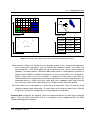
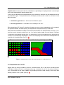
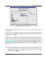
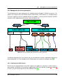
1
An introduction to the practical use
of the Free Geographical Information System
GRASS 6.0
Version 1.2
c 2004-2005 GDF Hannover bR
°
Imprint
This document is no original documentation of the described software. The software and hardware
descriptions named in this document are in most cases registered trademarks and are therefore
subject to the legal requirements. GRASS GIS is subject to the GNU General Public License. Find
more information on the GRASS GIS Homepage (12).
The details, data, results etc. that are given in this document have been written and verified to the
best of knowledge and responsibility of the editors. Nevertheless, mistakes concerning the content
are possible. Therefore, all data are not liable to any duties or guarantees. The editors and publishers
do not take any responsibility or liability for failures and their consequences. Your are always welcome
for indicating possible mistakes.
This document has been set with LATEX . It is available as LATEXsource code, online as HTML as well
as in printed version via the GDF Hannover bR (9).
The figures shown in this script are based on Free Geodata. The figures and the used software are
either liable to the Public Domain, the GNU General Public License or an appropriate license. Further
information concerning Free Software, GRASS GIS and Free Geodata can be found on the Internet
pages of the GRASS User-Association e.V. (GAV) (14), of the FreeGIS Project (16) and the Free
Software Foundation Europe (10).
Status: July 2005
c
Copyright °2004-2005
GDF Hannover bR
Editors:
Otto Dassau
Stephan Holl
Markus Neteler
Dr. Manfred Redslob
Translated by Kerstin Holl
Internet: http://www.gdf-hannover.de
Contact: [email protected]
Permission is granted to copy, distribute and/or modify this document under the terms of the GNU
Free Documentation License, Version 1.1 or any later version published by the Free Software Foundation; with no Invariant Sections. A copy of the license is included in the section entitled ”GNU Free
Documentation License”.
Contents
Contents
List of figures
vii
List of tables
ix
Preface
x
1 Introduction
1
2 Design and Structure
2.1 Geographical Data . . . . . . . . .
2.2 Data dimensions in GIS . . . . . .
2.3 The GRASS database . . . . . . .
2.3.1 The PERMANENT mapset
2.3.2 Design of further mapsets .
2.4 Command structure in GRASS . .
2.5 Help for using GRASS modules . .
2.6 GRASS variables . . . . . . . . . .
.
.
.
.
.
.
.
.
2
2
4
5
6
7
8
9
9
3 Installation of GRASS
3.1 Installation of a binary version
3.1.1 GRASS 5.4 . . . . . .
3.1.2 GRASS 6.0 . . . . . .
3.2 Installation from source code
3.3 Installation from CVS . . . . .
.
.
.
.
.
.
.
.
.
.
.
.
.
.
.
.
.
.
.
.
.
.
.
.
.
.
.
.
.
.
.
.
.
.
.
.
.
.
.
.
.
.
.
.
.
.
.
.
.
.
.
.
.
.
.
.
.
.
.
.
.
.
.
.
.
.
.
.
.
.
.
.
.
.
.
.
.
.
.
.
.
.
.
.
.
.
.
.
.
.
.
.
.
.
.
.
.
.
.
.
.
.
.
.
.
.
.
.
.
.
.
.
.
.
.
.
.
.
.
.
.
.
.
.
.
.
.
.
.
.
.
.
.
.
.
.
.
.
.
.
.
.
.
.
.
.
.
.
.
.
.
.
.
.
.
.
.
.
.
.
.
.
.
.
.
.
.
.
.
.
.
.
.
.
.
.
.
.
.
.
.
.
.
.
.
.
.
.
.
.
.
.
.
.
.
.
.
.
.
.
.
.
.
.
.
.
.
.
.
.
.
.
.
.
.
.
.
.
.
.
.
.
.
.
.
.
.
.
.
.
.
.
.
.
.
.
.
.
.
.
.
.
.
.
.
.
.
.
.
.
.
.
.
.
.
.
.
.
.
.
.
.
.
.
.
.
.
.
.
.
.
.
.
.
.
.
.
.
.
.
.
.
.
.
.
.
.
.
.
.
.
.
.
.
.
.
.
.
.
.
.
.
.
.
.
.
.
.
.
.
.
.
.
.
.
.
.
.
.
.
.
.
.
.
.
.
.
.
.
.
.
.
.
.
.
.
.
.
.
11
12
12
12
13
14
4 GRASS Project database
4.1 Calling up a GRASS project . . . . . . . . . . .
4.2 Projections . . . . . . . . . . . . . . . . . . . .
4.2.1 Geoid . . . . . . . . . . . . . . . . . . .
4.2.2 Ellipsoid . . . . . . . . . . . . . . . . . .
4.2.3 Datum . . . . . . . . . . . . . . . . . . .
4.2.4 Map projection types . . . . . . . . . .
4.2.5 Choosing the projection type . . . . . .
4.3 Examples of map projections . . . . . . . . . .
4.3.1 Azimuthal Projections . . . . . . . . . .
4.3.2 Conic Projections . . . . . . . . . . . . .
4.3.3 Cylindric Projections . . . . . . . . . . .
4.4 Coordinate systems . . . . . . . . . . . . . . .
4.4.1 Global coordinate systems . . . . . . .
4.4.2 2 and 3 dimensional coordinate systems
4.5 Creating different project regions in GRASS . .
4.5.1 Examples: Creating new project regions
.
.
.
.
.
.
.
.
.
.
.
.
.
.
.
.
.
.
.
.
.
.
.
.
.
.
.
.
.
.
.
.
.
.
.
.
.
.
.
.
.
.
.
.
.
.
.
.
.
.
.
.
.
.
.
.
.
.
.
.
.
.
.
.
.
.
.
.
.
.
.
.
.
.
.
.
.
.
.
.
.
.
.
.
.
.
.
.
.
.
.
.
.
.
.
.
.
.
.
.
.
.
.
.
.
.
.
.
.
.
.
.
.
.
.
.
.
.
.
.
.
.
.
.
.
.
.
.
.
.
.
.
.
.
.
.
.
.
.
.
.
.
.
.
.
.
.
.
.
.
.
.
.
.
.
.
.
.
.
.
.
.
.
.
.
.
.
.
.
.
.
.
.
.
.
.
.
.
.
.
.
.
.
.
.
.
.
.
.
.
.
.
.
.
.
.
.
.
.
.
.
.
.
.
.
.
.
.
.
.
.
.
.
.
.
.
.
.
.
.
.
.
.
.
.
.
.
.
.
.
.
.
.
.
.
.
.
.
.
.
.
.
.
.
.
.
.
.
.
.
.
.
.
.
.
.
.
.
.
.
.
.
.
.
.
.
.
.
.
.
.
.
.
.
.
.
.
.
.
.
.
.
.
.
.
.
.
.
.
.
.
.
.
.
.
.
.
.
.
.
.
.
.
.
.
.
.
.
.
.
.
.
.
.
.
.
.
.
.
.
.
.
.
.
.
.
.
.
.
.
.
.
.
.
.
.
.
.
.
.
.
.
.
.
.
.
.
.
.
.
.
.
15
15
19
19
19
20
20
22
22
23
23
23
24
24
24
25
26
GDF Hannover Courses
.
.
.
.
.
.
.
.
.
.
.
.
.
.
.
.
.
.
.
.
.
.
.
.
.
.
.
.
.
.
.
.
.
.
.
.
.
.
.
.
.
.
.
.
.
iii
Contents
4.5.2 Creating a Gauß-Krüger project region . . .
4.5.3 Creating a XY project region . . . . . . . .
4.5.4 Creating an UTM project region . . . . . . .
4.5.5 Creating a latitude-longitude project region
4.6 Deleting maps and projects . . . . . . . . . . . . .
.
.
.
.
.
26
29
29
30
31
5 Data import
5.1 Importing raster formats . . . . . . . . . . . . . . . . . . . . . . . . . . . . . . . . . . .
5.2 Importing vector data . . . . . . . . . . . . . . . . . . . . . . . . . . . . . . . . . . . . .
5.3 Importing sites . . . . . . . . . . . . . . . . . . . . . . . . . . . . . . . . . . . . . . . .
32
32
34
35
6 Georeferencing
6.1 Preparation for georeferencing . . . . . . . .
6.1.1 The optimal scan resolution . . . . . .
6.1.2 Creating the needed project regions .
6.2 Georeferencing procedure . . . . . . . . . . .
6.2.1 Choosing control points . . . . . . . .
6.2.2 Determining the correct transformation
.
.
.
.
.
.
38
38
38
39
40
40
42
7 Data export
7.1 Exporting raster formats . . . . . . . . . . . . . . . . . . . . . . . . . . . . . . . . . . .
7.2 Exporting vector data . . . . . . . . . . . . . . . . . . . . . . . . . . . . . . . . . . . .
7.3 Exporting sites . . . . . . . . . . . . . . . . . . . . . . . . . . . . . . . . . . . . . . . .
44
44
45
45
8 Graphical user interface
8.1 GIS Manager . . . . . . . . . . . . . . . . . . . . . . . . . . . . . . . . . . . . . . . . .
46
46
9 Working with raster data
9.1 Visualizing rastermaps . . . . . . . . . . . .
9.2 Query of raster cell values and metadata .
9.3 Different raster applications . . . . . . . . .
9.3.1 Calculating transects . . . . . . . . .
9.3.2 Line-of-sight-analysis . . . . . . . .
9.3.3 Overlapping of individual maps . . .
9.3.4 Buffering raster data . . . . . . . . .
9.4 Modification and assignment of colortables
9.5 Map statistics . . . . . . . . . . . . . . . . .
9.6 Methods for manipulating rastermaps . . .
9.6.1 Reclassification . . . . . . . . . . . .
9.6.2 Masking . . . . . . . . . . . . . . . .
9.7 Digitizing raster data . . . . . . . . . . . . .
49
50
51
53
53
53
54
55
56
57
59
59
60
61
GDF Hannover Courses
.
.
.
.
.
.
.
.
.
.
.
.
.
.
.
.
.
.
.
.
.
.
.
.
.
.
.
.
.
.
.
.
.
.
.
.
.
.
.
.
.
.
.
.
.
.
.
.
.
.
.
.
.
.
.
.
.
.
.
.
.
.
.
.
.
.
.
.
.
.
.
.
.
.
.
.
.
.
.
.
.
.
.
.
.
.
.
.
.
.
.
.
.
.
.
.
.
.
.
.
.
.
.
.
.
.
.
.
.
.
.
.
.
.
.
.
.
.
.
.
.
.
.
.
.
.
.
.
.
.
.
.
.
.
.
.
.
.
.
.
.
.
.
.
.
.
.
.
.
.
.
.
.
.
.
.
.
.
.
.
.
.
.
.
.
.
.
.
.
.
.
.
.
.
.
.
.
.
.
.
.
.
.
.
.
.
.
.
.
.
.
.
.
.
.
.
.
.
.
.
.
.
.
.
.
.
.
.
.
.
.
.
.
.
.
.
.
.
.
.
.
.
.
.
.
.
.
.
.
.
.
.
.
.
.
.
.
.
.
.
.
.
.
.
.
.
.
.
.
.
.
.
.
.
.
.
.
.
.
.
.
.
.
.
.
.
.
.
.
.
.
.
.
.
.
.
.
.
.
.
.
.
.
.
.
.
.
.
.
.
.
.
.
.
.
.
.
.
.
.
.
.
.
.
.
.
.
.
.
.
.
.
.
.
.
.
.
.
.
.
.
.
.
.
.
.
.
.
.
.
.
.
.
.
.
.
.
.
.
.
.
.
.
.
.
.
.
.
.
.
.
.
.
.
.
.
.
.
.
.
.
.
.
.
.
.
.
.
.
.
.
.
.
.
.
.
.
.
.
.
.
.
.
.
.
.
.
.
.
.
.
.
.
.
.
.
.
.
.
.
.
.
.
.
.
.
.
.
.
.
.
.
.
.
.
.
.
.
.
.
.
.
.
.
.
.
.
.
.
.
.
.
.
.
.
.
.
.
.
.
.
.
.
.
.
.
.
.
.
.
.
.
.
.
.
.
.
.
.
.
.
.
.
.
.
.
.
.
.
.
.
.
.
.
.
.
.
.
.
.
.
.
.
.
.
.
.
.
.
.
.
.
.
.
.
.
.
.
.
.
.
.
.
.
.
.
.
.
.
.
.
.
.
.
.
.
.
.
.
.
.
.
.
.
.
.
.
.
.
.
.
.
.
.
.
.
.
.
.
iv
Contents
10 Restructuring vector features
10.1 New properties of GRASS 6.0 . . . . . . . . . . . . . . . .
10.2 Management of vector geometries . . . . . . . . . . . . .
10.2.1 Working with OGR formats . . . . . . . . . . . . .
10.2.2 Creating geometries out of DBMS . . . . . . . . .
10.2.3 Creating geometries using XY and/or XYZ textfile .
10.3 Managing vector attributes . . . . . . . . . . . . . . . . . .
10.3.1 Display attributes . . . . . . . . . . . . . . . . . . .
10.3.2 Adding attributes . . . . . . . . . . . . . . . . . . .
10.3.3 Manipulating vector attributes . . . . . . . . . . . .
.
.
.
.
.
.
.
.
.
.
.
.
.
.
.
.
.
.
.
.
.
.
.
.
.
.
.
.
.
.
.
.
.
.
.
.
.
.
.
.
.
.
.
.
.
.
.
.
.
.
.
.
.
.
.
.
.
.
.
.
.
.
.
.
.
.
.
.
.
.
.
.
.
.
.
.
.
.
.
.
.
.
.
.
.
.
.
.
.
.
.
.
.
.
.
.
.
.
.
.
.
.
.
.
.
.
.
.
.
.
.
.
.
.
.
.
.
.
.
.
.
.
.
.
.
.
.
.
.
.
.
.
.
.
.
.
.
.
.
.
.
.
.
.
62
62
63
63
64
65
66
67
68
68
11 Working with vector data
11.1 Network analysis . . . . . . . . . . . . . .
11.1.1 Shortest-Path-Analysis . . . . . .
11.1.2 Subnets within a vector network .
11.1.3 Minimum-Steiner-Tree-Problem . .
11.1.4 Travelling-Salesman-Problem . . .
11.1.5 Cost analysis . . . . . . . . . . . .
11.2 Data intersection, data overlay, data union
11.2.1 Data union . . . . . . . . . . . . .
11.2.2 Data intersection . . . . . . . . . .
11.2.3 Data cutout . . . . . . . . . . . . .
11.2.4 Data overlay . . . . . . . . . . . .
11.3 Data extraction . . . . . . . . . . . . . . .
11.4 Data selection . . . . . . . . . . . . . . .
11.5 Topology management . . . . . . . . . . .
11.6 Digitizing with GRASS . . . . . . . . . . .
.
.
.
.
.
.
.
.
.
.
.
.
.
.
.
.
.
.
.
.
.
.
.
.
.
.
.
.
.
.
.
.
.
.
.
.
.
.
.
.
.
.
.
.
.
.
.
.
.
.
.
.
.
.
.
.
.
.
.
.
.
.
.
.
.
.
.
.
.
.
.
.
.
.
.
.
.
.
.
.
.
.
.
.
.
.
.
.
.
.
.
.
.
.
.
.
.
.
.
.
.
.
.
.
.
.
.
.
.
.
.
.
.
.
.
.
.
.
.
.
.
.
.
.
.
.
.
.
.
.
.
.
.
.
.
.
.
.
.
.
.
.
.
.
.
.
.
.
.
.
.
.
.
.
.
.
.
.
.
.
.
.
.
.
.
.
.
.
.
.
.
.
.
.
.
.
.
.
.
.
.
.
.
.
.
.
.
.
.
.
.
.
.
.
.
.
.
.
.
.
.
.
.
.
.
.
.
.
.
.
.
.
.
.
.
.
.
.
.
.
.
.
.
.
.
.
.
.
.
.
.
.
.
.
.
.
.
.
.
.
70
70
71
72
72
72
72
73
73
74
74
74
74
75
75
76
12 Application example: vector-based optimization of operation areas
12.1 Importing example data . . . . . . . . . . . . . . . . . . . . . . . .
12.2 Extracting hospitals from the point file . . . . . . . . . . . . . . . .
12.3 Assigning hospitals to the roadnet . . . . . . . . . . . . . . . . . .
12.4 Assignment of the regions of optimal achievability . . . . . . . . . .
.
.
.
.
.
.
.
.
.
.
.
.
.
.
.
.
.
.
.
.
.
.
.
.
.
.
.
.
.
.
.
.
.
.
.
.
.
.
.
.
.
.
.
.
85
85
87
87
89
13 Data conversion
13.1 Vectorization of raster data . . . . . . . . . . . . . . . . . . . . . . . . . . . . . . . . .
13.2 Converting vector data into the raster model . . . . . . . . . . . . . . . . . . . . . . . .
92
92
94
14 Data interpolations
14.1 Data interpolation into the raster model . . . . .
14.1.1 Inverse Distance Weighted . . . . . . . .
14.1.2 Regular splines with tension interpolation
14.2 Data interpolation into the vector format . . . . .
96
96
96
97
97
GDF Hannover Courses
.
.
.
.
.
.
.
.
.
.
.
.
.
.
.
.
.
.
.
.
.
.
.
.
.
.
.
.
.
.
.
.
.
.
.
.
.
.
.
.
.
.
.
.
.
.
.
.
.
.
.
.
.
.
.
.
.
.
.
.
.
.
.
.
.
.
.
.
.
.
.
.
.
.
.
.
.
.
.
.
.
.
.
.
.
.
.
.
.
.
.
.
.
.
.
.
.
.
.
.
.
.
.
.
.
.
.
.
.
.
.
.
.
.
.
.
.
.
.
.
.
.
.
.
.
.
.
.
.
.
.
.
.
.
.
.
.
.
.
.
.
.
.
.
.
.
.
.
.
.
.
.
.
.
.
.
.
.
.
.
.
.
.
.
.
.
.
.
.
.
.
.
.
.
.
.
.
.
.
.
.
.
.
.
.
.
.
.
.
.
.
.
.
.
.
.
.
.
.
.
.
.
.
.
.
.
.
.
.
.
.
.
.
.
.
.
.
.
.
v
Contents
15 Raster map arithmetic with r.mapcalc
15.1 Operators in r.mapcalc . . . . . . .
15.2 Features in r.mapcalc . . . . . . .
15.3 Internal variables in r.mapcalc . . .
15.4 Masking . . . . . . . . . . . . . . .
.
.
.
.
.
.
.
.
.
.
.
.
.
.
.
.
.
.
.
.
.
.
.
.
.
.
.
.
.
.
.
.
.
.
.
.
.
.
.
.
.
.
.
.
.
.
.
.
.
.
.
.
.
.
.
.
.
.
.
.
.
.
.
.
.
.
.
.
.
.
.
.
.
.
.
.
.
.
.
.
.
.
.
.
.
.
.
.
.
.
.
.
.
.
.
.
.
.
.
.
.
.
.
.
.
.
.
.
.
.
.
.
.
.
.
.
99
99
100
101
101
16 3D visualization and animation
103
16.1 Displaying a 3D map with NVIZ . . . . . . . . . . . . . . . . . . . . . . . . . . . . . . . 103
16.2 Displaying raster-volume-layers (VOXEL) . . . . . . . . . . . . . . . . . . . . . . . . . 105
16.3 Creating an animation . . . . . . . . . . . . . . . . . . . . . . . . . . . . . . . . . . . . 107
17 Visualizing and creating maps ready for press
17.1 Map export into a postscript-map . . . . . . .
17.2 Map export with PNG-driver . . . . . . . . . .
17.3 Creating shading effects . . . . . . . . . . . .
17.4 Processing maps with Xfig . . . . . . . . . . .
17.5 Processing maps with Skencil . . . . . . . . .
18 QGIS
18.1 Working with vector- and raster data
18.2 Visualizing and categorizing . . . . .
18.3 Editing . . . . . . . . . . . . . . . . .
18.3.1 GRASS vectordata . . . . . .
18.3.2 Shapefile . . . . . . . . . . .
18.4 GRASS Toolbox . . . . . . . . . . .
18.5 Processing GPS data . . . . . . . .
18.6 Geospatial bookmarks . . . . . . . .
18.7 Creating analog maps with QGIS . .
.
.
.
.
.
.
.
.
.
.
.
.
.
.
.
.
.
.
.
.
.
.
.
.
.
.
.
.
.
.
.
.
.
.
.
.
.
.
.
.
.
.
.
.
.
.
.
.
.
.
.
.
.
.
.
.
.
.
.
.
.
.
.
.
.
.
.
.
.
.
.
.
.
.
.
.
.
.
.
.
.
.
.
.
.
.
.
.
.
.
.
.
.
.
.
.
.
.
.
.
.
.
.
.
.
.
.
.
.
.
.
.
.
.
.
.
.
.
.
.
.
.
.
.
.
.
.
.
.
.
.
.
.
.
.
.
.
.
.
.
.
.
.
.
.
.
.
.
.
.
.
.
.
.
.
.
.
.
.
.
.
.
.
.
.
.
.
.
.
.
.
.
.
.
.
.
.
.
.
.
.
.
.
.
.
.
.
.
.
.
.
.
.
.
.
.
.
.
.
.
.
.
.
.
.
.
.
.
.
.
.
.
.
.
.
.
.
.
.
.
.
.
.
.
.
.
.
.
.
.
.
.
.
.
.
.
.
.
.
.
.
.
.
.
.
.
.
.
.
.
.
.
.
.
.
.
.
.
.
.
.
.
.
.
.
.
.
.
.
.
.
.
.
.
.
.
.
.
.
.
.
.
.
.
.
.
.
.
.
.
.
.
.
.
.
.
.
.
.
.
.
.
.
.
.
.
.
.
.
.
.
.
.
.
.
.
.
.
.
.
.
.
.
.
.
.
.
.
.
.
.
.
.
.
.
.
.
.
.
.
.
.
.
.
.
.
.
.
.
.
.
.
.
.
.
.
.
.
108
108
111
111
112
116
.
.
.
.
.
.
.
.
.
117
117
120
121
122
123
124
125
125
126
19 Definition of Free Software
128
20 GNU Free Documentation License
131
21 Command-Index
139
Cited literature
155
GDF Hannover Courses
vi
List of Figures
List of Figures
1
2
3
4
5
6
7
8
9
10
11
12
13
14
15
16
17
18
19
20
21
22
23
24
25
26
27
28
29
30
31
32
33
34
35
36
37
38
Roadmap of the GRASS development since 2001 (Status 1/2005) . . . . . . . . . . .
Geometry and attribute data within Geographical Information Systems . . . . . . . . .
Comparison of raster and vector data types in an identical area . . . . . . . . . . . . .
Data dimensions in GIS . . . . . . . . . . . . . . . . . . . . . . . . . . . . . . . . . . .
Example structure of a GRASS 6.0 database . . . . . . . . . . . . . . . . . . . . . . .
Innovations between GRASS 5.4 and 6.0 . . . . . . . . . . . . . . . . . . . . . . . . .
TclTk start screen in GRASS . . . . . . . . . . . . . . . . . . . . . . . . . . . . . . . .
Screen for defining a new Location in GRASS . . . . . . . . . . . . . . . . . . . . . . .
Screen for integrating an EPSG code . . . . . . . . . . . . . . . . . . . . . . . . . . . .
Projection of the earth’s surface on a map . . . . . . . . . . . . . . . . . . . . . . . . .
Various projection models (cylindric, conic and azimuthal) . . . . . . . . . . . . . . . .
Specifications to the extent of the project region and grid resolution . . . . . . . . . . .
Implementation of georeferencing in GRASS . . . . . . . . . . . . . . . . . . . . . . .
Searching control points of a scanned topographical map with the GRASS module
i.points . . . . . . . . . . . . . . . . . . . . . . . . . . . . . . . . . . . . . . . . . . .
d.m - GIS Manager of GRASS 6.0 including FRIDA data . . . . . . . . . . . . . . . . .
Representation of different line-transects of a relief model with d.profile . . . . . . . .
Buffering raster data with r.buffer . . . . . . . . . . . . . . . . . . . . . . . . . . . . . .
Representation of the GRASS 6.0 vector architecture . . . . . . . . . . . . . . . . . .
VMAP0 data Germany . . . . . . . . . . . . . . . . . . . . . . . . . . . . . . . . . . . .
Digitizing GUI of the module v.digit . . . . . . . . . . . . . . . . . . . . . . . . . . . .
Topographical map of the Spearfish region including landuse information . . . . . . . .
Creating an attribute table during digitization . . . . . . . . . . . . . . . . . . . . . . .
Attribute entry during digitization . . . . . . . . . . . . . . . . . . . . . . . . . . . . . .
Settings of the snapping threshold during digitization . . . . . . . . . . . . . . . . . . .
Basemap: Roads and hospitals of Osnabrueck . . . . . . . . . . . . . . . . . . . . . .
Assignment of the next achievable roads to the hospitals . . . . . . . . . . . . . . . . .
Modules for converting raster data into vector data . . . . . . . . . . . . . . . . . . . .
Smoothing vectorized data . . . . . . . . . . . . . . . . . . . . . . . . . . . . . . . . .
Modules for converting vector data into raster data . . . . . . . . . . . . . . . . . . . .
NVIZ graphical control window . . . . . . . . . . . . . . . . . . . . . . . . . . . . . . .
Volume-panel for volume-layer visualization . . . . . . . . . . . . . . . . . . . . . . . .
Different precipitation levels above Slovakia . . . . . . . . . . . . . . . . . . . . . . . .
Creating a simple animation in NVIZ . . . . . . . . . . . . . . . . . . . . . . . . . . . .
Simple result map ps.map (Soil map with legend in the Spearfish region) . . . . . . . .
Creating simple shading effects with d.his . . . . . . . . . . . . . . . . . . . . . . . . .
Processing simple map layouts with Xfig . . . . . . . . . . . . . . . . . . . . . . . . . .
Range of interesting drawing and editing features in Xfig . . . . . . . . . . . . . . . . .
Simple map layout with Xfig at the example of the geological map from the Spearfish
region . . . . . . . . . . . . . . . . . . . . . . . . . . . . . . . . . . . . . . . . . . . . .
GDF Hannover Courses
1
3
4
5
6
11
16
17
17
19
21
28
38
41
46
54
56
63
73
76
79
80
82
84
86
90
92
93
94
103
105
106
107
110
112
113
114
115
vii
List of Figures
39
40
41
42
43
44
45
46
47
48
49
50
Skencil with Geo-Object-Plugin at the example of the FRIDA-dataset of Osnabrueck
QGIS-Screenshot . . . . . . . . . . . . . . . . . . . . . . . . . . . . . . . . . . . . .
Alpha-Blending is supported by default . . . . . . . . . . . . . . . . . . . . . . . . . .
Dialog of the supported projections . . . . . . . . . . . . . . . . . . . . . . . . . . . .
Define your own projection . . . . . . . . . . . . . . . . . . . . . . . . . . . . . . . .
Properties of the vector layer . . . . . . . . . . . . . . . . . . . . . . . . . . . . . . .
QGIS in the editing mode of a GRASS vector map . . . . . . . . . . . . . . . . . . .
Starting and stopping the editing process . . . . . . . . . . . . . . . . . . . . . . . .
QGIS-Toolbox . . . . . . . . . . . . . . . . . . . . . . . . . . . . . . . . . . . . . . . .
QGIS-GPS plugin . . . . . . . . . . . . . . . . . . . . . . . . . . . . . . . . . . . . .
Geospatial bookmarks . . . . . . . . . . . . . . . . . . . . . . . . . . . . . . . . . . .
"Map Composer" for creating analog maps from QGIS . . . . . . . . . . . . . . . . .
GDF Hannover Courses
.
.
.
.
.
.
.
.
.
.
.
.
116
117
118
119
120
121
122
124
124
125
126
127
viii
List of Tables
List of Tables
1
2
3
4
5
6
7
8
9
10
11
12
13
14
15
Structure of the GRASS module names . . . . . . . . . . . . . . . . . . . . . . . . . .
9
Dimensions of some internationally used ellipsoids and examples of their usage locations 20
Some datums with their general application . . . . . . . . . . . . . . . . . . . . . . . . 20
Examples of azimuthal map projections . . . . . . . . . . . . . . . . . . . . . . . . . . 23
Examples of conic map projections . . . . . . . . . . . . . . . . . . . . . . . . . . . . . 23
Examples of cylindric map projections . . . . . . . . . . . . . . . . . . . . . . . . . . . 23
GRASS modules for importing raster data . . . . . . . . . . . . . . . . . . . . . . . . . 33
GRASS modules for importing vector data . . . . . . . . . . . . . . . . . . . . . . . . . 34
Polynomial degrees for georeferencing . . . . . . . . . . . . . . . . . . . . . . . . . . . 43
A range of modules for exporting raster data . . . . . . . . . . . . . . . . . . . . . . . . 44
A range of modules for exporting vector data . . . . . . . . . . . . . . . . . . . . . . . 45
Operators in r.mapcalc . . . . . . . . . . . . . . . . . . . . . . . . . . . . . . . . . . . 99
Features in r.mapcalc . . . . . . . . . . . . . . . . . . . . . . . . . . . . . . . . . . . . 100
Internal variables in r.mapcalc . . . . . . . . . . . . . . . . . . . . . . . . . . . . . . . 101
GRASS digitization tools (according to (8)) . . . . . . . . . . . . . . . . . . . . . . . . 123
GDF Hannover Courses
ix
Preface
Extensive support material is provided in the context of their tutorials by GDF Hannover bR (9). In
this way, the participants can apply the knowledge acquired through the exercises and examples to
daily use - even after finishing the course.
The content of this book is based on the GDF Hannover bR course titled:
An introduction in the practical use with
the Free Geographical Information System
GRASS 6.0
This book is mostly based on the longtime experiences of our internal and external employees, of
being used as teaching material at the University of Hanover and of the cooperation in the GRASSDevelopment Team. Corresponding to our company philosophy we always endeavor an active contribution for promoting, distributing and advancing Free (GIS)-Software. For this reason, all chapters of
this book are published according to the GNU Free Document License and are available on the GDF
Hannover bR (9) website.
The topics of our beginners courses are chosen depending on the respective duration as well as on
the specific ambitions of the participants. The individual chapters are therefore designed to provide
an overview of the basic functions of the GRASS system, and do not refer to any specific examples
or contents of GRASS courses of the GDF Hannover bR.
This book is meant to be a compact and clear introduction to GRASS 6.0 and quickly inform the reader
about the basic functions of the program. For more insight in the software, see the appropriate book
titles of the respective topics indicated in the bibliography.
GDF Hannover - Solutions for spatial data analysis and remote sensing
Hanover, July 2005
1 Introduction
Today, Free Software has become a synonym for innovation and progress. Free use, modification,
and distribution of the programs and their open source codes are guaranteed due to the support
of free idea exchange between users and developers. This means a steady, worldwide organized
and demand-oriented advancement in short periods of time for the Geographical Information System
GRASS GIS.
This document offers a short introduction in the Geographical Information System GRASS. It extends the known German and English literature ((5),(6)) by aspects of the use and the installation
of GRASS 6.0. In addition, modified material for using the latest GRASS developments is therefore
handed out from the date of publication.
Before reading this script we want to introduce you a little insight and view in the future of GRASS
GIS by the help of a Roadmap (Fig. 1) . It shows the directions in which GRASS development has
been moved since 2001 and will move in the future.
Roadmap GRASS GIS Development
5.1.x
CVS
5.0.x
CVS HEAD
5.0/5.1 code mix
6+
CVS HEAD
2003
5.1.x
2001
5.3.x
m
er
5.0.x
CVS release branch
ge
m
5.7
de
co e
r
g
o
aj er
m m
5.8.0
6.0
2003
er
ge
5.4.x
CVS release branch
5.0.2
5.0.3
5.4.0
Figure 1: Roadmap of the GRASS development since 2001 (Status 1/2005)
GDF Hannover Courses
1
2 Design and Structure
GRASS is a hybrid and modular structured GIS with raster-oriented and vector-oriented functions.
Each function of GIS is conducted by its own module. Thus, GRASS GIS is clearly structured and
seems very transparent. Another advantage of this modularity is that only the necessary modules
are running, which preserves the resources of the computer.
2.1 Geographical Data
GIS is characterized by four main components (1):
• Input
• Administration
• Analysis
• Presentation
The discussed data types of this four-component model are classified in three categories such as
geometry data, attribute data and graphics data with the following properties:
Geometry data describe the spatial situation of objects concerning their form and their relative situation in space. Usually, the spatial relation of individual points, lines or areas is made via the integration
in a coordinate system resulting in the relation to the real world and the metrics. Geometry data can
be available as raster data (pixel) or vector data (polygons / areas, lines, sites)(see Fig. 2).
Raster data are data continuously spread in space, which are structured in a measured matrix of
usually quadratic cells and cells with the same size. Each cell gets an attribute (property, attribute date), which represents an appropriate phenomenon (e.g. temperature or color value).
The storage of the cells is carried out by their coordinates. They are adjusted in rows and
columns. The geometrical data are accessed via the geographical coordinates or by specifying
the row and/or column. Working with raster data allows the application and analysis of remote
sensing data such as color infrared images of aerial operations, satellite photographs/images
and more. The necessary memory requirements and the appropriate high demand on computing resources (cpu time), which rise exponentially with the increase of resolution, is to be seen
as a disadvantage of raster data. Due to steady increasing CPU-power and larger storagecapacities this disadvantage has become less important over the last few years. Additionally,
raster data are not associated with so called neighborhood relationships because each pixel is
defined by its own situation in the coordinate system.
GDF Hannover Courses
2
2.1 Geographical Data
Rasterdata
10 23 23 35 35 44 67 88 88
y 52 4 25 18 −5
Vectordata
y
x
x
Pointdata
y
attribute data
x
x
x
x
x
xx
x
x
x xx
x
x
x
y
3595555
3595249
5774906
5774455
Lts
Lts
3595009
5774123
Ls
3595867
3595339
5774983
5774445
Su
Ls
3595889
5774101
Lts
x
Figure 2: Geometry and attribute data within Geographical Information Systems
Vector data are used for the storage of line information and/or for the storage of homogeneous
areas at closed lines (polygons). One line connects two end points (nodes) each, which also
have coordinates. Each vector object can be assigned with none, one or several attributes
(property). For administation in GRASS the dBase data-format is used by default. Interfaces to
different external DBMSs (Database Management System) like data bases e.g. PostgreSQL,
MySQL, Oracle and so on are also available. In comparison to raster data, vector data are
characterized by their comparatively low memory requirements and short computing times for
conducted analyses. Unlike raster data, vector data have a topology, which means that the
lines and areas "know" which nodes they possess and/or on which areas they border.
Point data (Sites) can be considered as a special form of vector data. They are used for saving
selectively spread spatial information. This data type can be saved as vector sites in GRASS
6.0 but not in version 5.4. Accordingly, it has the properties of vector data.
Attribute data (categories) are attributes, which are interconnected with the data types mentioned
above. They are mostly saved within GIS or in a database system coupled with GIS via DBMI
(Database Management Interface).
GDF Hannover Courses
3
2.2 Data dimensions in GIS
Graphics data eventually describe the method how a spatial object is displayed under a certain topic
on a certain output device (monitor, plotter, etc.).
In GIS, they are qualitatively and quantitatively set in relation as specimen via the combination of the
described data types. These phenomenons and objects (entities) to be saved in a GIS occur in two
basic structures:
• continuous appearances -> laminar and unlimited in space
• discrete appearances -> definable areas and objects like lines
When designing a GIS "correct" selection of the data structures to be used depends on the standard,
the spatial resolution, the data quantity, the original data, the planned analysis and more.
Within GRASS GIS different modules allow conversion between the individual data structures. Contour lines can be stored as vector lines, e.g. in a laminar terrain model (in raster format). Similarly,
a map consisting of digital contour lines (in vector format) can be transformed into a closed terrain
surface in raster format by interpolation. In this case the quality of the conversion will depend on the
resolution of the original data (see Fig. 3).
Raster− and vector−visualisation of identical spatial objects in GIS
1
1
1
1
1
1
2
2
2
1
1
1
1
1
2
2
2
2
1
1
1
1
1
2
2
2
2
3
3
3
3
1
2
2
2
2
1
1
1
3
3
2
2
2
2
1
1
1
1
3
3
3
2
2
1 = greenland
2 = water
1
2
3
1
3 = urban area
Figure 3: Comparison of raster and vector data types in an identical area
2.2 Data dimensions in GIS
Spatial data are mostly available as laminar, two-dimensional (2D) or two and a half-dimensional
(2.5D) data. Whenever there is a third parameter (e.g. elevation), we call this two and a half dimensions. Descriptions for the sides of bodies (e.g. building surfaces or floor sweeps) are the only data
actually saved as a 3D system (see Fig. 4).
GDF Hannover Courses
4
2.3 The GRASS database
Point
0D
Line
1D
Area
2D
Surface
2.5D
Face
3D
Figure 4: Data dimensions in GIS
2.3 The GRASS database
Geodata are internally saved by GRASS in a standard subdirectory called a GRASS database. In
most cases a new folder (e.g. grassdata/) is created in the users’s Home directory before GRASS
is installed for the first time:
cd
# Linux changes automatically to the Home directory
# of the user
mkdir grassdata # Compiling the subdirectory for the GRASS database
A subdirectory tree (Location) will automatically be created in GRASS for each project region defined
in GRASS. All project data are saved in the Location subdirectory. The Location can be further
subdivided into map subdirectories called (mapsets). This is how GRASS controls the organization
and the access to the data (see chapter 2.3.1 and 2.3.2).
GDF Hannover Courses
5
2.3 The GRASS database
GRASS Database
Location
Mapset
Geometry− and attribute data
cats
/prov_bz
/meran
/huber
cell
cellhd
cell_misc
/europa
/home/user/grassdata
/hannover
colr
/kronsberg
fcell
hist
/world
/europe
roads
forest
vector
water
poi
coor
dbln
hist
sidx
topo
roads.dbf
dbf
forest.dbf
water.dbf
poi.dbf
Figure 5: Example structure of a GRASS 6.0 database
Since different components (geometry, attribute and graphics data) of the individual layers are stored
in different subdirectories, all management of the project data should be done using GRASS commands, i.e. all file operations (copy, delete, rename) should be conducted with the appropriate
GRASS commands (g.copy, g.remove, g.rename)
2.3.1 The PERMANENT mapset
All information about projection, resolution and extent of the project area are stored within the compiled location in the PERMANENT mapset, which is automatically generated by GRASS. If necessary
the core data (original maps) of the project can be stored here because only the user who created
the new project has write permissions. Due to the internal structure it is guaranteed that the data can
not be changed by other users.
Other GRASS users and naturally the person who has write permissions for the PERMANENT
mapset should create additional mapsets for creating, saving and changing their own files and
analysis results based on the core data in the PERMANENT mapset.
GDF Hannover Courses
6
2.3 The GRASS database
Files in the PERMANENT mapset
The access to a single mapsets can be controlled individually for each project (Location) in GRASS.
If no maps (core data) are saved in PERMANENT it will only contains files with information about the
project area:
DEFAULT_WIND
Specifications of the edge coordinates, extension and resolution
of the environment PERMANENT
MYNAME
Name of the project -> e.g.: hanover
PROJ_INFO
Specifications of the projection -> e.g. tmerc (Transverse Mercator Projection), bessel (ellipsoid), potsdam (date)
PROJ_UNITS
Specifications of the units used e.g.: meter
WIND
Specifications of the current REGION and of the MAPSET projection
VAR
Specifications of the database driver and path
2.3.2 Design of further mapsets
Each GRASS user can create one or several mapsets in which he administers his own project data.
They can have the extent of the whole project or smaller.
This characteristic of the GRASS database structure makes it possible to work with several users
on one project at the same time e.g. in computer networks, without running the risk of changing or
destroying another user’s data. The mapsets of the other users can be specifically integrated in the
users ’own project’ by granting read-only permission. The resulting maps of any analysis are saved
in the mapset of the users current GRASS session.
GDF Hannover Courses
7
2.4 Command structure in GRASS
Mapset file structure
cats/
cell/
Category values (e.g. color or temperature values) and attributes
(classes with caption) of the individual raster maps
Individual raster maps
cellhd/
Header rows of the individual raster maps
cell_misc/
Statistical data of the individual raster maps
colr/
Color information of the individual raster maps
dbf/
Contains the internal vector attributes in DBASE format
fcell/
Raster maps with floating point numbers (f: floating point)
hist/
’Developing history’ of the individual raster maps
vector/
Contains the individual vector data (geometry, topology, etc.)
WIND
Data of the current REGION and the MAPSET projection
GRASS 6.0 allows one user to start several GRASS sessions in parallel.
2.4 Command structure in GRASS
The commands follow a very clear structure in GRASS. The type of a command can be recognized by
the abbreviation in front of the first period (prefix). Commands, which are independent programs are
called modules in GRASS. They have self-describing names. Thus, the module for digitalizing raster
maps is called r.digit. In order to convert vector data into raster format the module v.to.rast is
used. Table 1 describes the structure of the names of GRASS commands and modules in detail.
Modules and programs under GRASS
Apart from the modules existing in GRASS, all Unix/Linux programs are available. They can be
recalled via Shell, the command interpreter. This is particularly useful if you are interested in
programming, integrating or modifying your own and/or available GRASS modules. Even if it may
seem difficult to the beginner the ability of a user to program in GRASS provides nearly unrestricted
possibilities to realize their own needs and imagination within GIS. In addition, creating simple
Unix/Linux Shell scripts is easy to learn.
GDF Hannover Courses
8
2.5 Help for using GRASS modules
Table 1: Structure of the GRASS module names
Prefix
d.*
r.*
i.*
v.*
g.*
p.*
ps.*
db.*
Function class
display
raster
imagery
vector
general
paint
postscript
database
Meaning of the commands
For graphical display and visual query at the monitor
For raster data processing
For image processing
For vector data processing
General file operation commands
Map design commands
Map design commands for postscript size
Database management modules
r3.*
voxel raster
For 3D raster data processing
2.5 Help for using GRASS modules
A help file is available for nearly all of the 400 GRASS modules in which the command and the syntax
are described. For using a module a short help is available using the parameter: “ -help”.
d.rast -help
Detailed descriptions and examples of a module that correspond to the help pages on the GRASS
Homepage can be displayed with the command g.manual module name.
g.manual d.rast
Thereby, a browser is started, which displays the helping text. An overall index is also integrated into
the help, which is also available at the end of this booklet (see chapter 21).
2.6 GRASS variables
During a GRASS-session some variables are set. The can be printed and modified with the module
g.gisenv.
If the module is called without parameters, GRASS displays the current environment variable settings:
g.gisenv
GISDBASE=/home/holl/grassdata
GRASS_DB_ENCODING=utf-8
MAPSET=PERMANENT
LOCATION_NAME=spearfish
GRASS_GUI=tcltk
GDF Hannover Courses
9
2.6 GRASS variables
To display the current mapset, the module needs to be called with the parameter ’MAPSET’: g.gisenv
MAPSET
To modify a variable, use the following syntax:
g.gisenv set=’OVERWRITE=1’
This will set the variable OVERWRITE to overwrite-mode, which is deactivated by default.
A detailed list of GRASS-specific variables can be found at the help-pages:
g.manual variables
Note: Besides the currently mentioned variable ’OVERWRITE’ it is also possible to force the vectorand rastermodules to overwrite maps by using the switches -o or -overwrite (with two minus-signs).
So it it possible to force overwriting during each command individually, but default maps are still write
protected.
GDF Hannover Courses
10
3 Installation of GRASS
Three different variants can be chosen when deciding to install GRASS GIS on your computer. Although this book is an introduction into GRASS version 6.0, installation of the version 5.4 will be
discussed briefly. The choice of which version to install depends on the requirements of the user and
the applications that are necessary for the project work with GRASS GIS. The GRASS versions can
be described as follows:
• GRASS 5.4 : This version finishes the development of the official GRASS 5.x series. It is used
for production work in companies for many years now. It can surely be considered as a very
robust and stable version. GRASS 5.4 covers all raster functionality of GRASS 6.0.0, but not
the new vector functionalities. For users who only need raster functionalities, GRASS 5.4 is a
save choice.
• GRASS 6.0 : This GRASS version is the most recent GRASS version, which is released early
2005. It is based on the development version 5.7 and includes all known raster functionalities of
version 5.4 and the newly developed vector library. The development of GRASS is continuing
on the basis of GRASS 6.0. Therefor we like to encourage the users to use and test the
version 6.0; this is necessary for further development.
The GDF Hannover bR only uses this version for its work.
GRASS 5.4
GRASS 6.0.0
Raster− and imageanalysis
2D and 3D visualisation
d.dm /tcltkgrass
d.m / module GUIs
Pointdata (sites) support
Points (sites) as vectors
2D vector support (old vect)
2D/3D vector support
Datum Transformation
Vector network analysis
DBMS support
Spatial Index
Figure 6: Innovations between GRASS 5.4 and 6.0
The following descriptions are related to the installation on GNU/Linux systems. Thus, they are
accordingly modified transmissible on other platforms. Each stables version will shortly be described.
GDF Hannover Courses
11
3.1 Installation of a binary version
3.1 Installation of a binary version
GRASS versions 5.4 and 6.0 can be downloaded from the official GRASS GIS homepage (12) as
binary versions. Additionally GDF Hannover bR offers RPM-packages for recent GNU/Linux distributions.
3.1.1 GRASS 5.4
Like mentioned before, the GRASS Version 5.4.0 is officially released at the 5th of november 2004. In
comparison to version 5.0 they include important further developments of raster functionalities. The
newly developed vector library is not included, it is only part of GRASS 6.0.
A binary version is based on the official source code of the GRASS Version 5.4.0 and has been
precompiled on different computing and operating systems according to special guidelines. Thus,
GRASS can be installed on your computer without additional compiling in most cases. This needs a
compatible binary version for your system available and further necessary libraries are installed for
interacting with GRASS.
In this place we want to illustrate the installation of a binary version. A binary version of GRASS
5.4.0 is presently available for GNU/Linux systems. This version has also been precompiled on a
GNU/Linux system according to defined criteria. The descriptions of the system and used parameter
for precompiling can be found in the appropriate download area.
Therefor the program and the appropriate installation script need to be downloaded into an arbitrary
directory before installing the version with root permissions:
su
*****
sh grass5.4.0_i686-pc-linux-gnu_install.sh \
grass5.4.0_i686-pc-linux-gnu_bin.tar.gz
If the requirements differ from these requirements, it is necessary to compile the present source code
of the version GRASS 5.4.0 on your own computer. This procedure can be useful because the binary
version mostly does not include all features and modules (e.g. external database support).
The GRASS 5.4.0 source code and the related binaries can be downloaded directly from the Internet
pages of the GRASS GIS Homepage (12).
3.1.2 GRASS 6.0
The install procedure is identical to GRASS 5.4 and will be mentioned here (see chapter 3.1.1).
GDF Hannover Courses
12
3.2 Installation from source code
Again, the program and the appropriate installation script need to be downloaded into an arbitrary
directory before installing the version with root permissions:
su
*****
sh grass6.0.0_i686-pc-linux-gnu_bin.tar.gz \
grass6.0.0_i686-pc-linux-gnu_bin.tar.gz
If the requirements differ from these requirements, it is necessary to compile the present source code
of the version GRASS 6.0.0 on your own computer. This procedure can be useful because the binary
version mostly does not include all features and modules (e.g. external database support).
After a successful installation GRASS 6.0 can be started from the command-line by typing grass60
.
3.2 Installation from source code
For the case that it is necessary to compile the source code of the GRASS versions 5.4 or 6.0 on
your own computer, we shortly want to explain this procedure with an example. It should be taken
into account that this requires a little experience in compiling as well as studying of the installation
helps for installing GRASS without any problems in the required version.
The compiling and the installation is conducted with the “rule of proportion”, which is common for
Unix after the downloaded source code is unpacked.
./configure [...]
make
make install
Thereby, it needs to be considered that the pathes of additional programs and libraries must also be
indicated when entering the command ./configure. An example for keeping GDAL and PostgreSQL
support could be the following:
./configure --with-gdal=/usr/local/bin/gdal-config \
--with-postgres-includes=’/usr/include/pgsql /usr/include/pgsql/server/’\
--with-postgres-libs=/usr/lib
make
make install
A detailed description of the configuration parameters offers the command ’./configure –help’.
GDF Hannover Courses
13
3.3 Installation from CVS
Examples of configurations can be downloaded from the Website of the GDF Hannover bR (9) under
http://www.gdf-hannover.de/download or from the GRASS Homepage (12).
3.3 Installation from CVS
Another variant is to download the source code of the GRASS versions 5.4 or 6.0 as a tarballed
CVS snapshot from the GRASS Homepage (12) or directly from CVS. For the latter the CVS-needed
environment variable CVSROOT has to be set. Afterwards log into the CVS server, which asks for a
password and download the current source code on your computer and compile it like described in
chapter 3.2.
The following example shows this for a bash-Shell:
export CVSROOT=:pserver:[email protected]:\
/home/grass/grassrepository
cvs login
PW is "grass"
Now, a copy of the source code can be downloaded with the following command:
cvs -z3 co grass
cvs -z3 co grass51
# for GRASS 5.4 CVS
# for GRASS 6.0 CVS (according to
# historical reasons 5.1)
Subsequently this is compiled (see Chapter 3.2).
./configure [...]
make
make install
Within the folder grass or grass51 an update of the source code can be downloaded with the following
command in order to compile again:
make distclean
cvs up -dP
# Remove the already compiled parts of the source code
# Update the source code from the CVS
GDF Hannover Courses
14
4 GRASS Project database
In the GRASS database spatially-oriented data are managed geocoded. For this purpose a coordinate system (e.g.: Gauß-Krüger, UTM, etc.) of the project region, the so called Location, needs to be
decided upon before starting to work. Consider the following: As a rule, it is indispensable to choose
the structure and organization of the database to be used in GRASS and each GIS.
Extent of the project region: All the data that are to be imported as part of a project must be
contained within the spatial extent of the the Location. In addition one must determine what
projection is to be used for the project. This is usually provided with the data to be used in the
project and includes information about the projection such as projection name, ellipsoid, datum,
and other parameters.
Data resolution of raster data: In general, the computing and storage requirements increase
exponentially with resolution. However, if the resolution is lower than that of the dataset, there
will be data loss and the resulting GIS will be less than satisfactory. Therefore, it is useful to
choose the standard resoultion (default) to be equal to the resolution of the most important data
layers. The raster resolution can always be adjusted once the region has been created. When
importing data, the original resolution and map size is preserved.
Now that the properties of the project region and the data resolution have been determined, the next
step is to create a subdirectory for the GRASS database. This is usually called ’grassdata’ (see
chapter 2.3).
4.1 Calling up a GRASS project
If the start script of the version GRASS 6.0 is in the path ($PATH), GRASS can be started within an
open command interpreter (X-Terminal) via the command grass60 . A more detailed description can
be found in chapter 3.
The resulting start screen is shown in which some data must be entered via mouse or keyboard. A
graphical or text-based variant can be chosen by setting the parameter -text or -gui when starting
GRASS (see Fig. 8 and 7).
grass60 -text
grass60 -gui
# text-based start screen
# graphical start screen
GDF Hannover Courses
15
4.1 Calling up a GRASS project
Figure 7: TclTk start screen in GRASS
Here, an existing Location and mapset can be chosen from the menu or a new Location and mapset
can be created.
If a new mapset is to be added to an existing Location, first choose the appropriate Location, then
enter the name of the new mapset in the window below the text ’Create New mapset’ and click the
button ’Create ...’ (see Fig. 7).
There are three ways to create a new Location. (A) The projection data can be provided directly by
the user. The necessary information can usually be found in the metadata associated with the data
file. (B) The projection can be assigned automatically by entering the appropriate EPSG code (see
http://www.epsg.org/). This assigns standard projection and national grid systems parameters to
the Location. The appropriate code number can be found in the menu (see Fig.9) or as metadata.
(C) The projection data can be imported directly with the data by using the importmodules r.in.gdal
and v.in.ogr.
(A): In order to define the projection of a Location itself click with the mouse on the button ’Create
New Location’. GRASS ’changes’ to the text-based mode, which can also be your start screen
- depending on the start settings (see Fig. 8). The data for creating a new Location are entered
as described in chapter 4.5.1.
GDF Hannover Courses
16
4.1 Calling up a GRASS project
Figure 8: Screen for defining a new Location in GRASS
(B): If an EPSG code is exists for the project Location, it can be used to create a new Location
automatically. Click with the mouse on the button ’Create Location from EPSG’ and enter the
appropriate code number (see Fig. 9). The button ’EPSG Codes’ lists existing codes with their
appropriate definitions.
Figure 9: Screen for intergating an EPSG code
(C): In some cases, the data already contain all necessary projection information. It is thus possible
to generate a new Location during a running GRASS session using the projection information
GDF Hannover Courses
17
4.1 Calling up a GRASS project
contained in the data set to be imported. For example, a new Location can be created with a
SHAPE file or a GeoTIFF file, if a ’correct’ projection file (.prj) is available (unfortunately this
is rarely the case).
Example: Content of a SHAPE projection file (.prj)
PROJCS["Transverse Mercator",GEOGCS["bessel",
DATUM["Deutsches_Hauptdreiecksnetz",
SPHEROID["bessel",6377397.155,299.1528128],
TOWGS84[590.5,69.5,411.6,-0.796,-0.052,-3.601,8.30]],
PRIMEM["Greenwich",0],UNIT["degree",0.0174532925199433]],
PROJECTION["Transverse_Mercator"],PARAMETER["latitude_of_origin",0],
PARAMETER["central_meridian",9],PARAMETER["scale_factor",1],
PARAMETER["false_easting",3500000],PARAMETER["false_northing",0],
UNIT["meter",1]]
Example: Projection data of a raster map (GeoTiff)
Driver: GTiff/GeoTIFF Size is 3570, 3753 Coordinate System is:
PROJCS["Transverse Mercator",
GEOGCS["Deutsches_Hauptdreiecksnetz",
DATUM["Deutsches_Hauptdreiecksnetz",
SPHEROID["bessel",6377397.155,299.1528128000033],
TOWGS84[590.5,69.5,411.6,-0.796,-0.052,-3.601,8.3]],
PRIMEM["Greenwich",0],
UNIT["degree",0.0174532925199433]],
PROJECTION["Transverse_Mercator"],
PARAMETER["latitude_of_origin",0],
PARAMETER["central_meridian",9],
PARAMETER["scale_factor",1],
PARAMETER["false_easting",3500000],
PARAMETER["false_northing",0],
UNIT["meters",1]]
Origin = (3368561.280000,5928333.120000)
Pixel Size = (0.32000000,-0.32000000)
Corner Coordinates:
Upper Left ( 3368561.280, 5928333.120) ( 7d 1’12.86"E, 53d28’18.24"N)
Lower Left ( 3368561.280, 5927132.160) ( 7d 1’14.67"E, 53d27’39.41"N)
Upper Right ( 3369703.680, 5928333.120) ( 7d 2’14.77"E, 53d28’19.26"N)
Lower Right ( 3369703.680, 5927132.160) ( 7d 2’16.56"E, 53d27’40.43"N)
Center
( 3369132.480, 5927732.640) ( 7d 1’44.71"E, 53d27’59.33"N)
GDF Hannover Courses
18
4.2 Projections
It is important that such information is precisely controlled and scrutinized and that they should be
available as completely as possible. Small deviations, an incorrect DATUM or SPHEROID, can produce
enormous deviations in data positioning.
4.2 Projections
Before creating your own project region (Location) it is important to consider which projection will
be used. The following chapters will give a brief introduction to the most common projections, their
properties, and parameters.
Figure 10 shows the steps involved in deriving a map projection from real spatial data.
z
y
x
Geoid
Ellipsoid
Projection to
to plain area
Area with
coordinates
Figure 10: Projection of the earth’s surface on a map according to (7)
4.2.1 Geoid
A more precise definition of the earth’s shape, especially of the heights can be made via the identification of the geoid. This considerably more complex physical calculation results from the quantity
of the earth masses, which occur differently strong from region to region and therefore have different
gravitation forces, which affect on the earth’s shape. Thus, the geoid represents the gravitation field
of the earth. In case of the view in Figure 10 the shape of the earth looks really ’distorted’. Due
to the mathematical complexity the earth’s shape is usually displayed by ellipsoids in Geographic
Information Systems.
4.2.2 Ellipsoid
The simplified acceptance of the earth in spherical shape (sphere) is not exactly enough for creating
maps in higher scales than 1:2 Mio. Rotation ellipsoids or else spheroids try to readjust the complex
form of the earth mathematically as exactly as possible. Thereby, the distance between the poles
GDF Hannover Courses
19
4.2 Projections
and the geocenter is smaller than between the equator and the geocenter (see Fig. 10).
There is a range of ellipsoid models existing that should give optimized results for the different regions
of the earth. In general, a sufficient exact basic for the localization of the situation will be possible.
Table 2: Dimensions of some internationally used ellipsoids (data rounded) and examples of their usage
location according to (7)
Earth dimension
according to
Semi-major axis
(m)
Semi-minor axis
(m)
Usage location
Bessel 1841
6377397
6356079
Clarke 1880
Hayford 1909
6378249
6378388
6356515
6356912
WGS 1984
6378137
6356752
Germany,
Chile,
Netherlands,
Sweden, ...
Afrika, France
Belgium, Finland, Italy,
Spain, ...
North America, worldwide
4.2.3 Datum
There are numerous surveying points that are indicated as Datum and that can be calibrated by their
heights data. The following table contains a few examples for global and also regional datums. The
versions GRASS 5.4 and 6.0 both support datum transformation (see Fig. 6).
Table 3: Some datums with their general application
Datum
WGS 84
NAD 1983
European 1950
Region
Global
North America, the
Caribbean
Europe, North Afrika
Point of origin
Ellipsoid
Mass center of the earth
Mass center of the earth
WGS 84
GRS 80
Potsdam
International
4.2.4 Map projection types
In order to transfer the 3 dimensional form of the earth into a 2 dimensional plane (to project), a
projection is needed.
GDF Hannover Courses
20
4.2 Projections
cylindric
conic
azimuthal
Figure 11: Various projection models (cylindric, conic and azimuthal)
Depending on the regional situation different models are available (see Fig. 11) in order to hold the
unavoidable distortions as low as possible.
Cylindric Figure: This is the simplest of these figure variants. In this figure the map plane at
the equator is lain around the globe in order to create a cylinder. Meridians and parallels are
projected on the plane in such a way that a rectangular grid is created during the ’phase out’.
This figure is especially used for displaying regions near to the equator. A transverse variant is
also common in other regions.
Conic Figure: If a cone is lain over the earth and is unrolled in the plane, a conic figure is created.
With the simplest and most frequent application the apex lies on one line with both geographical
poles and illustrates the pole nearby. Thence, the meridians go off in the same angle and the
parallels form concentric circles around the intersection. The cone contacts the globe on one
or two parallels, the standard parallels. This form is frequently applied to figure regions in the
middle latitudes.
Azimuthal Figure: Here, the map plane is put on the earth’s shape as tangent. Imagine a source
of light in infinite distance at the opposite side shining through the globe and projecting the
shadows of the parallels and meridians on the map plane.
The basic projections represented here can additionally be varied by the situation of the illustration
plane to the earth. Normal (0◦ to the axis of the earth), oblique (45◦ to the axis of the earth) or
diagonal axial (90◦ to the axis of the earth).
GDF Hannover Courses
21
4.3 Examples of map projections
4.2.5 Choosing the projection type
The decision for a projection depends on the illustration properties needed in the project. Despite
the fact that a map projection is generally never displayable without distortions of one or several
characteristics (area, form, distance, scale, direction or relation) it must be specified before, which
properties have priority at the planned usage of the geodata.
Orthomorphic Projection: The scale remains the same from one point in all directions. The meridians and parallels intersect by 90◦ . The scale is locally the same and thus the form of the areas
remain. Additionally, the angles between the lines remain unchanged. These maps are mainly
used in the navigation and the surveying technology.
Equal-area Projection: Here, the area dimensions remain scaled as well as the proportional relations of the areas also remain. Scale, form and angle are distorted. The meridians do not
intersect the parallels in the right angle. But this is not very important concerning smaller areas.
These projections are often used for land use mapping and population mapping as well as for
other researches that are related to one specific area.
Equidistant Projection: The distance between sites on the map remains undistorted on equidistant
illustrations. This is especially important for traffic maps.
4.3 Examples of map projections
Some examples of the different projection types and their characteristics are named in table 4, 5 and
6. Further information concerning this topic can be found in (2) and (3).
GDF Hannover Courses
22
4.3 Examples of map projections
4.3.1 Azimuthal Projections
Table 4: Examples of azimuthal map projections
Type
Genomic
Stereographic
Orthographic
Light source
Vanishing point at the
geocenter
Vanishing point opposite to the projection
center
Vanishing point so far
away that radiation
dips in parallel
Properties
true-to-scale, where
meridians and parallels cross, neither
orthomorphic
nor
equal-area
orthomorphic, true-toscale, where meridians and parallels
cross
only true-to-scale in
the projection center,
neither orthomorphic
nor equal-area
Circular regions
In case of satellite impages
Application
4.3.2 Conic Projections
Table 5: Examples of conic map projections
Type
Lambert Conformal Conic
Albers Equal-Area Conic
Properties
Orthomorphic
Equal-area
Application
For large-scale and middle-scale
maps of the middle latitudes
The parallels stand in pole proximity
closer together than at the equator;
is still often used in the USA today.
4.3.3 Cylindric Projections
Table 6: Examples of cylindric map projections
Type
Mercator
Transverse Mercator Projection
Figure
Normal axial projection
Mercator projection rotated 90◦
Properties
Orthomorphic, parallel distances
increase proportionally from the
equator to the scale
Orthomorphic
Application
For navigation and illustrations near
to the equator
Recommended for regions with N-S
extent (G-K, UTM basic)
GDF Hannover Courses
23
4.4 Coordinate systems
4.4 Coordinate systems
Having projected the globe or a part of it on a plane, a coordinate system must be inserted in order
to place 2 or 3 dimensional sites exactly on the map. In general, global and 2 dimensional and/or 3
dimensional coordinate systems are to be differentiated.
4.4.1 Global coordinate systems
Longitude-Latitude: The most frequently used global system is that of the longitude, latitude, and of
the height (here: it concerns no projection). The reference planes are the 0 meridian and the equator.
The earth is therefore divided into 180 longitudes from Greenwich to the East and West. Beginning at
the equator, the earth is also divided into 90 latitudes to the South and North. The height is measured
at the geocenter but accordingly definition differences are still existing. The units of the system can
be specified in the sexagesimal- (Degree:Minutes:Seconds, letter index to the orientation) or decimal
system (pos./neg. degree with decimal places).
4.4.2 2 and 3 dimensional coordinate systems
In order to specify sites numerically on a map projection, rectangular (cartesian) coordinates are
used - where the positive y-values are pointed to the East and the positive x-values are pointed to
the North. The zero point is differently defined in each system - in GRASS usually in the left edge
below. In contrast to geographical and geocentric coordinates sites are only available for one defined
illustration range (e.g. meridian stripes). Numerous coordinate systems are applied internationally.
Besides different zero points and dimension units different ellipsoids and projections are chosen as
basis. This results in the fact that a transformation is mostly only possible via a complex calculating
operation.
In GRASS several modules are available for this purpose (r.proj and v.proj). Now, we briefly
want to introduce theoretical examples of the Gauß-Krüger and UTM coordinate systems, which are
used in Germany.
Gauß-Krüger coordinate system
This meridian stripe system has been established in Germany in 1927. The Bessel ellipsoid is the
chosen land survey datum, the transverse mercator projection is the projection and potsdam is the
datum. The coordinates refer to one meridian stripe each, whereas the longitudes 6◦ , 9◦ , 12◦ and
15◦ as main meridians (x-axis) are valid in Germany. The distortion can be reduced to a maximum
of 12 cm per kilometer at the outer meridian stripes because a diagonal axial mercator projection is
conducted at each single meridian stripe. The extent complies to 100 km in each direction of the
main meridian. Thus, an overlapping of the individual meridian stripe systems of approx. 23 km
occurs. The northings on the main meridian are seen as the distance from the equator. In order to
GDF Hannover Courses
24
4.5 Creating different project regions in GRASS
avoid negative values with the easting the value +500000 m is adopted for the main meridian. Based
on this the distance in meters between a given point and the main meridian can be calculated by
reducing or adding 500000 from the easting value. A number derived by the decimal degree of the
main meridian divided by 3 is added at first order.
Northing is always calculated as distance from the equator.
Lüneburg lies e.g. in the system of the 9th longitude on 3593000/5902000 (easting/northing) and in
the system of the 12th longitude on 4392753/5902298 (easting/northing).
UTM coordinate system
The UTM System (Universal Transverse Mercator) is currently based on the WGS84 ellipsoid. The
earth is covered by 60 meridian stripes between 84◦ northern latitude and 80◦ southern latitude.
These stripes are 6 longitudes wide, each. An intersection cylinder is used for the projection in
order to avoid distortions of the longitudes at the border meridians. Thus, the central meridian is
not equidistant anymore but shows a diminution factor of 0,9996. At Gauß-Krüger the northing is
measured in kilometer as the distance of the point from the equator. On the contrary, 10000 km
are added on the southern hemisphere in order to avoid negative values. The distance from the
central meridian, which has the values 500km like at Gauß-Krüger is defined by the x-values. The
appropriate coordinates are indicated with E (East) and N (North). The central meridians can be
found at 3◦ , 9◦ , 15◦ and so on in eastern and/or western longitude. The zones are divided into
8 latitude stripes from the South pole to the North Pole and they are indicated with letters. This
system is used for military maps of the United States and of the NATO. According to the international
usability of the UTM coordinate system also Germany and/or Europe endeavor the introduction of
this coordinate system.
4.5 Creating different project regions in GRASS
After this excursion though the world of projections, which play an important role for working with
geographical information systems, it is time to introduce the process of defining project regions (Locations) in GRASS (see Chapter 4.1).
To create a Location the following parameters must be known:
1. Coordinate system (xy environment or environment with projection, ellipsoid and datum)
2. Area of interest (minimum and maximum coordinates of the work area)
3. Raster resolution (usually the most frequently occurring raster resolution)
GDF Hannover Courses
25
4.5 Creating different project regions in GRASS
4.5.1 Examples: Creating new project regions
After starting GRASS (see Chapter 4.1) click with the mouse on the button Create New Location for
creating a new location. Now, the text-based mode is opened (see Fig. 8). This is equivalent to
starting GRASS with the setting grass60 -text. When a session is ended, the start mode is saved
and become the default start mode. The start mode can be changed using the option grass60 -gui
or -text.
Three entries must be made in the start window to define a new Location.
LOCATION: The name of the project region to be created (e.g. Hanover).
MAPSET: The the name of a work area which is located within the Location (e.g. Kronsberg).
DATABASE: The full path to the GRASS database created using mkdir grassdata in which the
project data have to be saved (e.g. /home/user/grassdata).
Please remember: The mapset PERMANENT in which the general information of the project region
is saved in individual files will automatically be created by GRASS (see Chapter 2.3) – even if you
have entered an other name in the sector mapset.
Subsequently, the keystrokes <ESC><ENTER>, that is typical for GRASS, leads you to the screen
for defining the project region. The creation of a Gauß-Krüger Location is described in chapter 4.5.2.
The procedure for defining other coordinate systems is similar.
Advice: The values for the projection of a location can always be set on the previously defined default
values via the module g.region -d. While working with GRASS the module g.region -p lists the
projection and resolution values currently being used.
4.5.2 Creating a Gauß-Krüger project region
The Gauß-Krüger coordinate system uses a transverse mercator projection. Accordingly, the cylinder
- rotated 90◦ - is transversely put over the Bessel ellipsoid. Distortions occur in the border area (max.
12 cm/km on a length of 2◦ ). This means the Gauß-Krüger sheet sides are not displayed parallel to
the sides of the paper in topographical maps using this projection.
Now, the first task would be to choose the desired projection system from the menu. However, the
Gauß-Krüger system is not listed therefore we must select ’other ’. These are the steps to be followed:
For the Gauß-Krüger system:
- coordinate system for location:
GDF Hannover Courses
other (D)
26
4.5 Creating different project regions in GRASS
Followed by a short description of the project region:
- one line description for location: e.g.Hanover
Further data of the projection are now following:
-
specify projection name: tmerc (Transverse Mercator)
specify ellipsoid name: bessel (Bessel Ellipsoid)
Do you want to specify a map datum for this location? potsdam
Enter Central Parallel [lat_0] (23N): 0N
Enter Central Meridian [lon] (96W): 9E
Enter Scale Factor at the Central Meridian: 1
Enter False Easting: 3500000 (3 because 9E is Central Meridian)
Enter plural form of units: meters
During parameter input, it is sometimes possible to display the projection parameter supported by
GRASS via the entry list.
After the projection parameters have been entered, set border coordinates of the project region. The
boundaries are set to: North = 5801000, South = 5787000, West = 3427000, and East = 3445000.
The Gauß-Krüger values (defined exactly in meters) of the topographic maps are attached with 3
zeros. For more precision a point is following and afterwards the decimal places (see Fig. 12).
The specification for the resolution (raster cell in meters) in east-west and north-south direction
is entered in the same entry mask. This is the standard raster resolution (default) of the created
location. Thus, it has no importance for the sharply illustrated sites and vector data and can always
be changed with GRASS while working. It is recommended to take into consideration that the
resolution of raster data has an enormous influence on the necessary calculating and memory
requirements.
GDF Hannover Courses
27
4.5 Creating different project regions in GRASS
Figure 12: Specifications to the extent of the project region and grid resolution
As usual, complete the data entry by pressing <ESC><ENTER> and you will get back to the beginning. Confirm the creation of the mapset with "yes" because the name for the mapset was already
been indicated. An additional confirmation of all the data will finally exit this page. Now, the project
region is installed and active. This can be seen because GRASS Prompt is displayed in the Shell.
The command g.region -p can be used to verify the region data.
Here is an example of a Gauß-Krüger project region:
projection:
zone:
datum:
ellipsoid:
north:
south:
west:
east:
nsres:
ewres:
rows:
cols:
GDF Hannover Courses
99 (Transverse Mercator)
0
potsdam
bessel
5801000
5787000
3427000
3445000
2.5
2.5
5600
7200
28
4.5 Creating different project regions in GRASS
4.5.3 Creating a XY project region
Creating an xy-location, which is necessary for e.g. intermediate steps for geocoding of nonreferenced map scans, is much more simple because no projection parameters need to be provided.
After entering ’A’ at the question concerning the coordinate system
- coordinate system for location:
x,y (A)
it is directly be followed by the definition of the border coordinates (columns or width, rows or height)
of the project region. The border coordinates are defined by the pixel extent of the non-referenced
map(s) to be imported. These can be determined among other things with the program xv (Windows
-> Image Info). Starting from the defined attachment in the left edge below only a north and an east
value is added according to the rows and columns of the original picture. The raster resolution must
consequently be 1.
This procedure will be discussed again in the context of georeferencing a scanned map (see
chapter 6).
Here is an example of a XY project region (g.region -p):
projection:
zone:
north:
south:
west:
east:
nsres:
ewres:
rows:
cols:
0 (x,y)
0
8000
0
0
8000
1
1
8000
8000
4.5.4 Creating an UTM project region
The creation of an UTM location (Universal Transverse Mercator) resembles the creation of a
Gauß-Krüger location (but with a smaller cylinder). In this case, it is not referred to a "Berührzylinder"
with the basic bessel ellipsoid but to a "Schnittzylinder" with the basic WGS 84 ellipsoid. With respect
to the Gauß-Krüger projection, the parameters that have changed are shown below:
GDF Hannover Courses
29
4.5 Creating different project regions in GRASS
-
coordinate system for location: UTM (C)
specify ellipsoid name: z.B.: wgs84 (world geodetic system 1984)
do you want to specify a map datum for this location? z.B.: wgs84
Enter Zone 32 (UTM zone for Germany)
Is this South Hemisphere? n
Afterwards the coordinates of the project region are defined. The entry is in meters, which means a
7-digit number for the northern value and a 6-digit for the eastern value.
Here is an example of a UTM project region (g.region -p):
projection:
zone:
datum:
ellipsoid:
north:
south:
west:
east:
nsres:
ewres:
rows:
cols:
1 (UTM)
32
potsdam
wgs84
6100000
5880000
500000
630000
12.5
12.5
17600
10400
4.5.5 Creating a latitude-longitude project region
A latitude-longitude location contains data in latitudes and longitudes (0-90◦ north and/or south,
0-180◦ east and/or west), expressed in the sexagesimal system (degree:minutes:seconds, letter
indicating the orientation) or decimal system (pos./neg. decimal degrees). The entry of the border
coordinates and standard raster resolution can be in the decimal degrees system or sexagesimal
system.
- coordinate system for location:
latitude - longitude (B)
Here is an example of a lat-lon project region (g.region -p):
GDF Hannover Courses
30
4.6 Deleting maps and projects
projection:
zone:
datum:
ellipsoid:
north:
south:
west:
east:
nsres:
ewres:
rows:
cols:
3 (Latitude-Longitude)
0
unknown (default: WGS84)
unknown (default: WGS84)
90N
90S
180W
180E
0:04:48
0:04:48
2250
4500
4.6 Deleting maps and projects
In order not to destroy the internal structure of the GRASS database the command g.remove is to be
used for deleting single maps within a mapset! It is not recommended to delete files without sufficient
knowledge and it should never be carried out manually outside of GRASS or with UNIX commands
and/or programs in Linux. By using the command g.mremove it is possible to delete several maps at
the same time.
Exception: The deletion of a complete mapset and location. For this purpose, GRASS has to be
exit using the command exit. The command rm -r or a file manager (e.g. konqueror) can delete a
mapset and/or a location within the GRASS database.
Attention: Accordingly, all saved data (maps, files...)
mapset...) will be deleted!
of the respective directories (location,
For example: The command rm -rf ~/grassdata/Hanover irrevocably deletes without further enqueries the complete location named Hanover with all its containing mapsets.
GDF Hannover Courses
31
5 Data import
Before starting with the data import we should mention the model of the GRASS GIS data structure
(see chap. 2.3). The terminology used in this section is explained in detail in the model.
Interoperability is an important condition for working with GIS, for instance the import of raw data
or data conversion from other software packages. GRASS offers a large quantity of modules for
importing vector data, raster data, and sites. The specific command syntax can be displayed with the
-help parameter or the module g.manual.
v.in.ogr -help
g.manual v.in.ogr &
r.in.gdal -help
5.1 Importing raster formats
GRASS GIS supports the import of many different raster formats. Generally, three format types
should be considered.
Image format: The individual rasters always have positive, integral values in the known pixel-based
image formats such as PPM, PNG, JPEG, and GIF.
ASCII format: The individual rasters of the ASCII format can contain positive and negative, integral
values as well as floating point values. The ASCII-GRID of Arcinfo is an example of this format.
Binary format: In the binary raster format the individual pixels with positive and negative, integral
values or floating point values can also be saved in different channels with different resolutions.
(Geo)TIFF or ERDAS/IMG are examples for this format.
Now, it is time to mention a property of GRASS GIS related to raster data import: raster maps are
always imported with their original resolution and border coordinates but they are exported with the
current resolution and border setting of the region (see chapter 7.1).
For importing non-georeferenced data there are two cases to be considered:
1. If the location including resolution is defined and the map has to fit in, the scan resolution
complies with the required resolution (GRID RESOLUTION).
2. If the parameter of the location can comply with the map to be imported – especialy the resolution – it has to be installed in such a way that the image can be imported unchanged.
Table 7 gives a list of modules used to import raster data in different formats i.e. formats of other GIS
systems as well as special formats of other remotesensing sectors.
GDF Hannover Courses
32
5.1 Importing raster formats
Table 7: GRASS modules for importing raster data
GRASS
Module command
Import
Raster format
r.in.ascii
r.in.bin
GRASS ASCII
BIL, GMT binary files, LANDSAT TM5
r.in.gdal
ARC/INFO ASCII/Binary GRID, BIL, ERDAS (LAN, IMG),
USGS DOQ, JPEG, SAR CEOS, EOSAT, GeoTIFF,
PPM/PNM, SDTS DEM,
GIF, PNG
(see also http://www.gdal.org/formats_list.html)
Importing a GeoTiff file
The most frequently used module for importing raster data is r.in.gdal. As described in table 7, it
is able to read and write many different formats (r.out.gdal). As an example we will import a georeferenced map in ERDAS IMG format. We have prepared a small ASTERDEM of 30 m resolution
based on vector data of the city of Osnabrueck. This is available on the GDF Hannover bR website
(http://www.gdf-hannover.de/download).
r.in.gdal in=asterdem30m.img out=asterdem30m
Projection of input dataset and current location appear to match.
Proceeding with import...
100%
CREATING SUPPORT FILES FOR asterdem30m
COPYING COLOR TABLE FOR asterdem30m
With the flag -e a possibly necessary spacial extent of the location’s definition will be achieved.
# Adapting the current region to the map:
g.region rast=asterdem30m -p
The resulting map can be displayed using the Display Manager d.m or with the command d.rast.
For this purpose, a GRASS monitor has to be started before with d.mon x0.
# Starting the Display Manager
d.m&
GDF Hannover Courses
33
5.2 Importing vector data
# Displaying the map in the prompt:
d.mon x0
d.rast asterdem30m
5.2 Importing vector data
In the latest version 6.0 GRASS the vector libraries underwent a complete reorganization. This was
necessary because the GRASS version 5.4 had a strong focus on raster data and sites analysis. This
course will focus on the new GRASS version 6.0 vector functions. The changes to the vector format
can be found in chapter 10.
To import vector data it is essential to take a multitude of different format and standards into consideration. Compared to raster formats the structure of vector data is more complex. This makes vector
import more complicated. Table 8 lists the formats which are supported by GRASS GIS. Probably
the most frequently used format is the ESRI SHAPE format.
Once the vector file is imported, it will be available in the native GRASS binary vector format. The
geometries, topologies, and all attributes are stored in the internal GRASS database. A topology
is created for each map during the import. The current topology status can be displayed via the
command v.info. More vector related commands are described in chapter 10.
Table 8: GRASS modules for importing vector data
GRASS
Module command
Import
Vector format
v.in.ogr
SHAPE file, UK.NTF, SDTS, TIGER, S57, MapInfo-File,
DGN, VRT, AVCBin, REC, Memory, GML, ODBC
(see also: http://www.gdal.org/ogr/ogr_formats.html)
GRASS ASCII
ArcInfo-E00-format
Create vectors from database with x|y[|z] coordinates
v.in.ascii
v.in.e00
v.in.db
Importing a SHAPE File
The module for importing SHAPE data to GRASS is called v.in.ogr. Note that the SHAPE format
is not a topological format; there are no situation and/or neighbor relations between the individual
objects. For example, border lines between two areas (polygones) are saved twice. This may lead to
problems and therefore has to be corrected by GRASS during the import process.
The data for this exercise comes from the FRIDA project (17), which maintains a large quantity of
GDF Hannover Courses
34
5.3 Importing sites
detailed vector data of the city of Osnabrueck which are made available by Intevation GmbH (13).
v.in.ogr -o dsn=./frida-1.1-shp-joined/streets-joined.shp out=streets
12323 primitives registered
0 areas built
0 isles built
Number of nodes
:
8937
Number of primitives:
12323
Number of points
:
0
Number of lines
:
12323
Number of boundaries:
0
Number of centroids :
0
Number of areas
:
0
Number of isles
:
0
Within GRASS (under $GISDBASE/$LOCATION/$MAPSET) a subfolder named streets has been created
in the directory vector during the import. In this directory the topology (topo), the header information
(head), the vector geometries (coor), the history (hist), the spacial index (sidx), and the category
index (cidx) as well as a link to the corresponding attribute data (dbln) are stored.
According to the default the attribute data has been stored within GRASS in the directory dbf as
DBASE format - also during the import. If required, it is possible to have a look at the content of the
newly imported attribute table (streets.dbf) with an appropriate editor. Under GNU/Linux this can be
done with OpenOffice, Gnumeric or Koffice.
Other methods for importing vector data or generating vector data based on databases such as
PostgreSQL or PostGIS can be found in chapter 10.
If the vector data contain their own projection information, a new location can be created during a
GRASS session, which is based on this information. The necessary information of SHAPE data are
saved in the file with the ending .prj. Creating a new location with the import of the data has the
following syntax:
v.in.ogr dsn=./frida-1.1-shp-joined/streets-joined.shp \
out=streets location=osnabrueck
5.3 Importing sites
In GRASS 6.0 sites are no longer stored seperately in a directory site_lists but they are saved as
vector points and analysed with the vector modules. Vector sites that are for instance available as
SHAPE data will be imported with the module v.in.ogr like it is mentioned in the following example:
GDF Hannover Courses
35
5.3 Importing sites
v.in.ogr -o dsn=./frida-1.1-shp-joined/poi-joined.shp out=poi
268 primitives registered
0 areas built
0 isles built
Number of nodes
:
268
Number of primitives:
268
Number of points
:
268
Number of lines
:
0
Number of boundaries:
0
Number of centroids :
0
Number of areas
:
0
Number of isles
:
0
Importing Eastings and Northings (X|Y)
Often sites are given as eastings and northings in simple ASCII table to be imorted into GIS. For
this purpose, GRASS offers the module v.in.ascii. The sites should be listed in the order Easting
Northing Value. The separator plays no special role. For example, a file (coord.txt) shall be imported
whose columns are separated by the ’pipe’ sign:
1664619|5103481
1664473|5095782
1664273|5101919
cat coords.txt | v.in.ascii out=points
Missing category values (IDs) can be added after the fact using the v.category module, so that it is
possible to assign additional attributes to be stored in the database:
v.category in=punkte out=points2 op=add
v.category points2 op=report
The site information is then available as GRASS vector format in the current location in the folder
vector of the GRASS database.
Importing elevation data (X|Y|Z)
If a third column contains elevation data as the attribute, the parameter -z must be added to the
v.in.ascii command:
1664619|5103481|101.2
GDF Hannover Courses
36
5.3 Importing sites
1664473|5095782|102.2
1664273|5101919|101.7
cat coords3d.txt | v.in.ascii -z out=elevation
v.category in=elevation out=elevation2 op=add
v.category elevation2 op=report
Examples of how to extract sites from existing databases are given in chapter 10.
GDF Hannover Courses
37
6 Georeferencing
This chapter can be skipped, if no unreferenced data are to be imported.
In order to import scanned raster maps to be later georeferenced two project regions need to be
defined. The scanned maps are first imported in a XY location (without projection) and afterwards
"equalized" (geocoded) in a second location with a defined coordinate system.
GRASS target−location
with geocoding
GRASS XY−Location
without geocoding
Transformation
Geocoding
scaned "raw map"
i.group
i.target
i.points/i.vpoints
i.rectify
rectified result map
Figure 13: Implementation of georeferencing in GRASS
6.1 Preparation for georeferencing
The desired projection of the target location is to be defined before starting the equalization according
to the required geographical borders and resolution. In principle, any projection supported by GRASS
can be defined. The resolution of the target location should not be too low. If the resolution of the
target location is too low compared to the resolution of the data to be georeferenced, "resampling"
during the georeferencing process will result in a low quality digital map (data loss). On the other
hand, too high relative resolution will result in a high quality map requiring an unreasonable amount
of storage space (file size).
6.1.1 The optimal scan resolution
If an analog map is to be imported into GRASS GIS, the scan resolution of the map also determines
the resolution of the location which is to be chosen. This may seem very simple but requires some
trial and error to find the balance between not too high (file size) and not too low (data loss) scan
value. The following example shows how to proceed in order to adjust the location optimally on the
GDF Hannover Courses
38
6.1 Preparation for georeferencing
geodata (or vice versa):
a) Sample calculation of the resolution for a 300dpi scan:
300dpi = 300rows/2,54cm = 118,11rows/cm
b) Calculation of the compatible raster resolution for a 1:25000 map scale:
Route_in_nature/scan rows_per_cm = 25000cm/118,11rows = 2.12m/row
If the location with its resolution is already defined, a conversion between scan resolution and geographical resolution will be necessary to determine the value for the scan resolution. The example
shown above is thus counted back (5).
6.1.2 Creating the needed project regions
The first step is to create a XY location for the scanned raw map to be imported. The extent of the
project region should at least comply with the number of pixel in X-(rows, height) and Y-(columns,
width) direction of the map to be imported (e.g. use ’xv’ for determination). It is important that the
XY location be large enough to accomodate the raw data. GRASS allows the locations to be larger
than needed, so when in doubt it is possible to "play it safe" and define a generous location (storage
space does not cost extra!). The resolution is set to 1 so that each pixel of original image can be
assigned to a raster field in GRASS. Usually the geographical resolution (e.g. in meters) determines
the number of pixel of the scanned map. However, this connection is irrelevant in the projectionfree XY location. Only later, with the transformation to another coordinate system, will the "genuine"
resolution (specified by the scan resolution and the map scale) be assigned.
The second step is to create a target location into which the georeferenced map is to be transformed.
The target location will provide the projection, extent, and resolution required by the project. In the
simplest case a target location already exists to which the georeferenced map will be added. The
creation of a target location is described in chapter 4.5.1.
Procedure for several map segments
If a map consists of several segments, each segment should be imported independently into separate
XY locations in order to exclude "slips of the pen" during the georeferencing. Otherwise, the map can
be composed with an image editing program before importing into GRASS in order to import the map
"as a whole" - but only if the scans are properly cut. This is only recommended if the data to be
imported already lie properly one upon the other as image data. An example could be unreferenced
satellite images, which have been supplied congruently for different spectral ranges.
GDF Hannover Courses
39
6.2 Georeferencing procedure
6.2 Georeferencing procedure
Once the XY location with the raw map and the target location with the projection have been created,
we are ready to georeference the raw map as follows:
1. Indicate the name of the map and image data that are to be transformed into a newly created
image group.
i.group
• Assign names for this group: e.g. "map".
• Select the map(s) to be imported with an "x".
2. Indicate the target location (target) and mapset (e.g. a Gauß-Krüger location) in which the map
and image data shall be transferred.
i.target
• The target location should not be zoomed. Otherwise the end-product is only transferred
to the zoomed cutout because GRASS always works with the current region. Reset the
standard resolution (in the target location) as follows: g.region -dp
3. Start a GRASS monitor: d.mon start=x0
4. Assign the Gauß-Krüger coordinates to the four edges or coordinate-crosses of the region to
be transformed (see chapter: 6.2.1).
i.points (Related to raster maps)
i.vpoints (Related to vector maps)
• Indicate the image group to be transformed (for this example "map").
6.2.1 Choosing control points
The imported map/image is clickably displayed in the GRASS monitor on the left hand side. There are
two possibilities for georeferencing: either (A) using reference coordinates or (B) using an existing
reference map in the target location.
GDF Hannover Courses
40
6.2 Georeferencing procedure
Figure 14: Searching control points of a scanned topographical map with the GRASS module i.points
(A): If control points for georeferencing are known, e.g. from an available analog paper map, clearly
identifiable points such as Gauß crosses or indicated edge coordinates are chosen by clicking
on the imported map, and entering the coordinates in X term (separated by a space).
(B): If a georeferenced map exists in the target location, which exhibits distinctive points (such
as crossroads or buildings) and which can also be found in the map to be referenced, the
georeferenced map can be loaded into the right window with the ’PLOT RASTER’ function.
Thus, it is possible to find and to mark corresponding reference points in both monitor windows.
The ’ZOOM’ function allows exact placement of control points (see Figure 14).
The control points should be evenly distributed throughout the map. The RMS error can be determined via the ’ANALYSE’ function, which should not be higher than half of the raster resolution of
the target location. All partial RMS errors are calculated to an overall error. Where required, it is
GDF Hannover Courses
41
6.2 Georeferencing procedure
possible to ignore or reassign an inexactly assigned control point by double clicking on the point in
the ’ANALYSE’ function window. Points can be disconnected in this way to reduce the RMS error
or to redistribute the points more evenly.
An even distribution of points with "suboptimal" RMS error can produce an overall lower error than a
poor distribution of points with "optimal" RMS error.
The module i.points is exited after the successful assignment of the control and reference points.
The coordinate assignments are automatically saved on exit. This also applies to previously assigned
points, from prior executions of i.points. With a new call you can continue working on the same
location.
Depending on the original data and the selected polynomial degree of the equalization to be performed, the module i.rectify is started when sufficient points for georeferencing have been set. In
this context the group of images to be equalized must first be indicated. The query follows whether
the map
1. shall be transformed into the ’current region’ of the target location (complies with the currently
set parameters (cutout, resolution) of the target location);
2. or in the ’minimal region’ (GRASS independently calculates the range in the target location).
If in this menu point 1 ’current region’ is chosen, it is important to ascertain again before referencing
that the current settings of the target location (cutout and resolution) are correctly chosen. Due to the
fact that all data are automatically saved it is no problem to leave the module i.rectify and GRASS
again, to verify the current settings of the target location or to change if necessary, and to call the XY
location and i.rectify again.
6.2.2 Determining the correct transformation
The correct transformation is defined by the polynomial degree. This depends on the degree of
distortion (at central perspective aerial views e.g. by the relief energy existing in the project region) as
well as on the quorum of available control points. The greater the image-internal distortion the higher
the needed polynomial degree and the more control points are needed for an exact georeferencing
(see table 9). Too high polynomial degrees are however mathematically not reasonable.
As a rule of thumb correct internal image geometry (e.g. scanned topographical maps, as orthogonal projection) requires a minimal quantity of control points and therefore a minimal polynomial
degree. Otherwise, distorted internal image geometry (e.g. historical map) needs a higher quantity
of control points and therefore a higher polynomial degree.
GDF Hannover Courses
42
6.2 Georeferencing procedure
Table 9: Polynomial degrees for georeferencing
Polynomial degree
Minimum number of
Control points
1
2
3
4
3
6
10
15
Module
i.rectify
If too few reference points are set for a chosen polynomial degree, GRASS does not start the rectification. A guide for determining the minimum number of control points needed by polynomial degree is
given in table 9. Polynomial degrees of first to third order are proven of value. Whereby at polynomial
degrees of third order more than 10 control points are required.
GDF Hannover Courses
43
7 Data export
The data export is naturally just as important for working in GIS as the data import described in
chapter 5. There is a possibility between the export of data in exchange formats, which are further to
be processed with other GIS software, or the export in image formats for a professional visualization
with external graphic software such as Xfig or Skencil. GRASS offers a range of modules, which can
export raster data, vector data, and sites. The respective command syntax can be learned or – like
all the other modules – printed with the parameter ’-help’.
7.1 Exporting raster formats
In table 10 those modules are listed, which can export GRASS raster data into different external
formats. Besides this formats of other GIS systems and also special exchange formats of remote
sensing data belong to these modules.
Table 10: A range of modules for exporting raster data
GRASS
Module commands
Export
Raster formats
r.out.arc
r.out.ascii
r.out.mpeg
r.out.png
r.out.pov
r.out.ppm
r.out.tiff
r.out.bin
r.out.gridatb
r.out.gdal
ARC/INFO ASCII GRIDa
ASCII
MPEG
PNG (see also d.mon/PNG DRIVER with True Color Support)
POV
PPM/PNM
TIFF/TFW
Binary Array
GRIDATB.FOR (TOPMODEL)
Over 20 important formats are supported (see paragraph:
Export with GDAL)
a
Note: The Arc Toolbox in ArcGIS supports the import of ASCII-grids: Import to Raster -> ASCII to Grid. The result
can be selected in ArcCatalog. Be aware that the extension Spatial Analyst must be present and activated.
As mentioned in chapter 5.1 for exporting raster data the special characteristic of GRASS has to
be considered that raster maps are always exported with the current resolution and only for the just
determined region (current region). Thus, it is always advisable to ascertain in the forfront with the
command g.region -p, if the present settings of the ’region’ are correct before exporting, importing,
and analyzing raster data.
GDF Hannover Courses
44
7.2 Exporting vector data
Export with GDAL
The module r.out.gdal is able to export GRASS raster data into different formats. An appropriate
list can be displayed with the command r.out.gdal -l.
In order to use this module it is presently necessary to install GDAL with GRASS-Support. For this
purpose the ready-to-install binary-packages need to be installed. If no binary-package is available
for your platform, it needs to be built from source. Please obtain detailed information about this topic
from GDF Hannover bR.
7.2 Exporting vector data
In table 11 the available modules in GRASS are listed, which are able to export GRASS vector data
into different external vector formats.
Table 11: A range of modules for exporting vector data
GRASS
Module commands
Export
Vector formats
v.out.ascii
v.out.ogr
GRASS ASCII
SHAPE, TIGER, S57, MapInfo, DGN, Memory, CSV,
GML, ODBC and PostgreSQL
Povray
v.out.pov
7.3 Exporting sites
In GRASS 6.0 sites are considered as vectors. The known sites formats from GRASS 5.4 can still be
exported via the module s.out.ascii. Otherwise, the module v.in.sites is used in order to convert
existing sites data into the vector format and then to transform them into different export formats.
Exporting elevation data from raster maps
For exporting elevation data from a raster map into the xyz format it is necessary to adjust the resolution of the location to the resolution of the raster map. Afterwards, the X, Y and Z values will be
written into an ASCII file cell by cell.
g.region rast=elevation.dem -p
r.stats -1 -g input=elevation.dem > spearfish_elevation.txt
GDF Hannover Courses
45
8 Graphical user interface
In the field of GIS usability plays a more and more important role. Although GIS traditionally preferred
the prompt. From this point of view we want to go into the development of the graphical user interface
of GRASS GIS because a lot of innovations and updates have taken place in the last month and
years.
8.1 GIS Manager
Since GRASS 6.0 there is a further new GUI concept. On the one hand module-depending pop-up
menus, which open automatically when a module name without further parameters is entered in the
GRASS Shell, are part of this concept. On the other hand GRASS has been supplemented by a new
GIS manager. This manager contains a range of ordinary functions, which shall make the work with
the mouse clearer and more comfortable (see Figure 15). Furthermore all functions from TclTkGRASS
4.0 are integrated into the new GIS Manager.
Figure 15: d.m - GIS Manager of GRASS 6.0 including FRIDA data
The GIS manager can be started with the command d.m&. It also offers some special graphical
GDF Hannover Courses
46
8.1 GIS Manager
buttons besides the modules, which are clearly ordered like in the former TclTkGRASS 4.0 as pulldown menus. These refer to the sectors of visualization, attribute administration, digitization, and
printing and are situated with the pull-down menus on the basis of simple symbols beneath the
analysis bar.
Pull-down menus for the data analysis (GIS-Manager)
Approximately 200 of the 400 modules that are available in GRASS GIS are integrated in the pulldown menus. This offers the possibility that the most frequently used modules can easily be used
with the mouse. The menu’s structure is the following:
File: contains modules for importing and exporting data and for setting the project.
GIS: makes settings for the projection, the work environment and the data management possible.
Display: contains modules for visualizing raster data, vector data and sites.
Raster: contains modules for analyzing raster data.
Vector: contains modules for analyzing vector data.
Image: contains modules for analyzing image data.
Grid3D: contains modules for analyzing voxel data (3D raster data).
Databases: contains modules for querying and managing databases.
Help: Help functions.
Graphical buttons for simple visualization (Display Manager)
The graphical buttons that are situated under the pull-down menus allow rapid and intuitive visualization, query and management of available data. The functions are the following:
Display selected layers (current region): is used in order to display all in the display manager
chosen maps (see red box) in the current set ’region’ and ’resolution’.
Display selected layers (default region): is used in order to display all chosen maps in the total
extent ’default region’ and the defined ’default resolution’ (see g.region -d).
Display from saved region settings: is used in order to display maps in a previously defined extent
and resolution (see g.region -help).
Erase to white: is used for deleting the content of the current monitor in order to call a new map.
(see d.erase -help).
GDF Hannover Courses
47
8.1 GIS Manager
Zoom: allows to zoom in and/or out of map cutouts. Thus it is important to take the assignment of
the mouse buttons in the command interpreter into consideration.
Return to previous zoom: zooms to the previously selected region.
Pan and recenter: is used in order to pan in the currently displayed map. Please pay attention to
the notifications in the command interpreter.
Query map: allows to query for raster and vector maps. The results of the raster maps are shown
in the command interpreter, the results of the vector maps are visualized in a pop-up window
and can be modified according to the settings. The respective map must be chosen before.
Add group: is used in order to define a map group for visualization. This map group can be saved
as a kind of ’project’ wherever you like. It is recommended to save it in the directory of the
current mapset.
Add raster: makes the call of a new raster map possible.
Add vector: makes the call of a new vector map possible.
Add paint label: is used in order to integrate images into the map, which are stored in the
paint/labels folder (see v.label).
Create new command: makes possible to define commands or even command sequences which
can be recalled with a mouse-click.
Digitize vector map: is used in order to change the geometries of vector maps loaded in d.m. Thus,
the digitalizing module v.digit is started. The respective map must be chosen with the mouse
before.
Cut selection: allows to delete maps or also commands from the GIS manager. These maps are
still available in the location. For deleting maps from the databasis it is necessary to use the
module g.remove.
Create new workspace file: makes possible to create a kind of project file, in which maps are
saved including their color assignments, visualization sequence and so on.
Open an existing workspace file: is used in order to recall a project file, in which maps are saved
including their color assignments, visualization sequence and so on.
Save workspace file: is used in order to save a created project file, in which maps are saved
including their color assignments, visualization sequence and so on.
Print map: makes possible to save maps in different image formats. The current possible formats
are Postscript, PDF and PNG. The map is saved in the current extent and resolution.
GDF Hannover Courses
48
9 Working with raster data
From simple queries to complicated algebraic functions and logical conditions practically any analysis
and modeling are possible with raster data in GRASS GIS.
Due to the large number of raster data analysis modules currently available (more than 100) this
chapter will provide a general intoduction to raster data processing. The topic of remote sensing,
which means the processing and analysis of satellite and aerial images, is not part of this book, and
plays a subordinated role. Some literature concerning remote sensing analysis is specified in the
bibliography.
As described in chapter 8 most of the analyses can be executed using the graphical user interfaces
TclTkGRASS and GIS Manager. Here we will explain each step of the anaysis as a GUI operation
as well as a command-line instruction. The use of GRASS at the command-line prompt is highly recommended in order to familiarize the user with individual modules, their usage, and the parameters
they require.
General information concerning raster data
A raster value is defined by its localization coordinates x,y (cell center) and a z-value, which corresponds to a measurement or object value which is usually assigned a color or grey value when
displayed. Two basic operation types are available for creating thematic maps based on raster data:
1. pointwise, raster cell-oriented or pixel-oriented operation (neighborhood operations)
2. matrix-oriented or pixel window supported operation (moving-window-operations)
Besides using the "ready-to-go" GRASS modules, which each provide a particular operation,
solution-oriented operations of both types can be defined and applied via the arithmetic module
r.mapcalc (see chapter 15).
Raster data management
The basic management for the components of raster data like the spatial reference of maps, attribute
and color assignment of the pixel is directly conducted by each raster modules when executed.
Thus, the module r.support used in former versions (GRASS 5.0 and 5.3) is no longer necessary.
In addition, the creation of map statistics with the module r.support -r is only calculated for the
selected map cutout, which in most cases was not intended and led to unintentional effects.
Help functions to the GRASS modules
GDF Hannover Courses
49
9.1 Visualizing rastermaps
A help file is available for nearly all of the more than 400 GRASS modules. In this file the module is
described and command syntax explained. A short version of the help can be displayed by entering
the module command with the parameter -help at the prompt:
d.rast -help
A detailed help with a module description and examples, which is equivalent to the help pages on the
GRASS homepage, can be displayed by the command g.manual module name. For this purpose, a
standard browser is automatically opened and displays the corresponding help file:
g.manual d.rast &
9.1 Visualizing rastermaps
The visualization of raster data is conducted in a so called X monitor by the module d.rast. GRASS
can manipulate up to 7 different monitors (x0,x1,x2,..,x6) in parallel:
d.mon x0
d.rast
Use the d.zoom module to get a more detailed view of a regional cutout:
d.zoom
A particular cutout or the total work area can be defined via the module g.region. The setting of the
default region with a resolution of 10 m can be achieved using:
g.region -d res=10.0 -pa
d.erase
d.rast rastermap
Note that the settings changed by g.region must be passed to the monitor by the module d.erase
in order to be take effect. It is also possible to adjust region and resolution settings directly from a
raster map:
g.region rast=rastermap -p
d.redraw
Visual overlapping of two raster files
d.rast rastermap1
d.rast -o rastermap2
A pixel of the underlying rastermap1 is only visible if the corresponding pixel of the overlay rastermap2
contains a NULL-values, indicating a data gap. The module d.his also overlays maps – e.g. for the
visual verification of the georeferenced TK24 of the Spearfish sample dataset.
GDF Hannover Courses
50
9.2 Query of raster cell values and metadata
d.his -n h_map=roads i_map=tk24
Visualization of a rastermap with legend
A rastermap with appropriate legend can be displayed quickly by entering the following command:
d.rast.leg rastermap
9.2 Query of raster cell values and metadata
In order to get coordinates and raster attributes of individual pixels the module d.what.rast can be
run after displaying the raster map:
d.what.rast
It is also possible to query multiple rastermaps that have not been displayed:
d.what.rast map=elevation.dem,geology,soils
By clicking on a pixel with the mouse its characteristic values are displayed in the terminal window.
Also the attribute values of a pixel can be queried in several maps displayed in the monitor. Exit the
module by clicking the right mouse button.
r.info
The r.info module is used for displaying basic information and metadata information for the
rastermap. It also shows a data description, data type, the map projection, and the value ranges
of available categories.
r.info landuse
r.info -r landuse
r.cats
To control the attributes of a rastermap, create a table with assigned label numbers and appropriate
text attributes using the r.cats module:
r.cats map=landuse
1
residential
2
commercial and services
3
industrial
4
other urban
5
reservoirs
GDF Hannover Courses
51
9.2 Query of raster cell values and metadata
6
7
8
bare exposed rock
quarries, strip mines and gravel pits
transportation and utilities
r.report
To determine the area of individual geological units in the Spearfish region, for example, use the
r.report module as shown below (also see r.stats). This module calculates statistics based on the
current region and raster resolution settings. Therefore, zooming in prior to executing this command
will describe the cutout region only:
g.region rast=geology -p
r.report -h geology units=h
+---------------------------------------------------------------------+
|
Category Information
|
|
|#|description
| hectares|
|---------------------------------------------------------------------|
|1|metamorphic. . . . . . . . . . . . . . . . . . . . . . .| 1051.000|
|2|transition . . . . . . . . . . . . . . . . . . . . . . .|
13.000|
|3|igneous. . . . . . . . . . . . . . . . . . . . . . . . .| 3285.000|
|4|sandstone. . . . . . . . . . . . . . . . . . . . . . . .| 6755.000|
|5|limestone. . . . . . . . . . . . . . . . . . . . . . . .| 5537.000|
|6|shale. . . . . . . . . . . . . . . . . . . . . . . . . .| 4170.000|
|7|sandy shale. . . . . . . . . . . . . . . . . . . . . . .| 1019.000|
|8|claysand . . . . . . . . . . . . . . . . . . . . . . . .| 1307.000|
|9|sand . . . . . . . . . . . . . . . . . . . . . . . . . .| 3295.000|
|*|no data. . . . . . . . . . . . . . . . . . . . . . . . .|
168.000|
|---------------------------------------------------------------------|
|TOTAL
|26,600.000|
+---------------------------------------------------------------------+
r.timestamp
For processing time series it is often necessary to provide maps with a timestamp (time of creation,
data acquisition, and so on). For this purpose the module r.timestamp is used. Absolute and relative
dates can be indicated, which are stored independently from the file history:
r.timestamp landuse date="27 Sep 2003"
r.timestamp landuse date="27 Sep 2003/20 Feb 2004"
GDF Hannover Courses
52
9.3 Different raster applications
A more detailed description of the available timestamp formats can be found in the help file via
g.manual r.timestamp.
9.3 Different raster applications
GRASS is very extensive especially with regards to raster analysis. In this section we will introduce some of the more frequently used raster GRASS modules. The modules and the applications
discussed here represent only a few of those currently available.
9.3.1 Calculating transects
In order to display a (line-) transect in a raster diagram the menu-driven module d.profile can be
used (see Figure 16).
d.profile
Raster cell values or aggregated values in case of median and arithmetic average along one or more
transects can be listed in ASCII format using the module r.profile. It is possible to give coordinatepairs or interactively select start- and endpoint (option -i). The module r.transect provides a front
end to the r.profile module. It only needs the startpoint of the transect and calculates the endpoint
automatically based on the parameters azimuth and distance.
r.profile
r.transect
9.3.2 Line-of-sight-analysis
The r.los module performs a line-of-sight analysis based on an elevation map. A starting point,
the height above the ground at this point as well as the distance from this point up to which the
line-of-sight analysis is to be calculated can be indicated via a coordinate.
As an example, we will use the elevation map elevation.10m from the Spearfish data set. The initial
coordinate is specified in this case but can also be determined by the module d.where:
# Put the setting on relief model but 20m resolution
g.region rast=elevation.10m res=20 -pa
# Calculation of visibility of a tower 15m over terrain
# (computionally extensive at 10m original resolution...)
r.los in=elevation.10m out=visibility coord=593670,4926877 \
GDF Hannover Courses
53
9.3 Different raster applications
Figure 16: Representation of different line-transects of a relief model with d.profile
obs=15 max=30000
# Control
d.erase
r.shaded.relief elevation.10m units=meters
d.rast elevation.10m_shade
d.rast -o roads
d.rast -o visibility
9.3.3 Overlapping of individual maps
As already mentioned it is possible to overlay raster maps visually. However, the module r.patch
can be used to save the overlay as a new map. Thus, it is possible to combine several maps to a
single map via patching:
GDF Hannover Courses
54
9.3 Different raster applications
r.patch in=map1,map2,map3,map4 out=total map
The first map indicated lies on top. All other maps are successively placed under each other and only
appear in those places where the maps lying above have the value NULL (no data). As an example,
the geological map and the roadmap from the Spearfish data set are to be overlayed. It is important
to consider that GRASS modules basically work in the current region and resolution. Therefore the
region with its resolution and area must be adjusted to the maps to be patched.
g.region rast=geology,roads -p [res=12.5] [-a]
r.patch in=roads,geology out=roads.on.geol
If the order of the maps is changed, the entire roadmap is overlayed by the geological map. Such an
output map would ultimately be identical to the map geology.
9.3.4 Buffering raster data
The module r.buffer allows the user to define a buffer based on the raster data. This function can
be used for creating noise protection zones for the individual road categories of the map roads. Using
the Spearfish data set, first list the available categories:
# Which road categories are available?
g.region rast=roads -p
r.report -h roads
|1|interstate
|2|primary highway, hard surface
|3|secondary highway, hard surface
|4|light-duty road, improved surface
|5|unimproved road
|*|no data
Problem: To define buffer zones with distances of 100, 250 and 500 meters around the "interstate"
roads only. The initial map has a resolution of 30 m, which is maintained thoughout the exercise:
# Extracting the category ’interstate’ with r.reclass
r.reclass roads out=interstate << EOF
1 = 1 interstate
EOF
# or extracting the category ’interstate’ with r.mapcalc
r.mapcalc "interstate=if(roads==1,roads,zero())"
GDF Hannover Courses
55
9.4 Modification and assignment of colortables
# Creating buffer zones
r.buffer in=interstate out=interstate.buf dist=100,250,500
# Control
d.rast.leg interstate.buf
Figure 17: Buffering raster data with r.buffer
The resulting map shows the "interstates" with the three previously defined buffer zones. The specification of the buffer width is always referred to the middle of the feature to be buffered (in this case
interstate roads) and is calculated in map units (e.g. meters) defined by the location. The units can
be queried in GRASS via the module g.proj -p:
g.proj -p
...
-PROJ_UNITS-----------------------------------------------unit
: meter
units
: meters
meters
: 1.0
The conversion of a raster map into vector datamodel can be found in chapter 13.1.
9.4 Modification and assignment of colortables
The values available in an image file are visually coded by GRASS via a colortable. After creating
a raster image the rastermap is assigned to - with few exceptions - the default colortable “rainbow”.
There are several ways to create a map-specific colortable.
One of the standard colortables can be assigned using the module r.colors:
GDF Hannover Courses
56
9.5 Map statistics
r.colors map=raster map color=standard table
r.colors map=raster map color=special table
color options: aspect,grey,grey.eq,grey.log,byg,byr,gyr,rainbow,ramp,
random,ryg,wave,rules
rules options: aspect,bcyr,byg,byr,elevation,evi,grey,gyr,rainbow,ramp,
ryg,slope,srtm,terrain,wave
By indicating the variable rules we can assign our own colortable:
r.colors map=geology color=rules << EOF
4 100 200 0
5 255 130 7
6 100 129 187
7 222 180 39
9 43 18 200
EOF
For transferring the colortable from one rastermap to another or for assigning an individual or already
specified colortable use the module r.colors with the parameter "rast":
r.colors rastermap rast=orig_rastermap
The newly assigned colortable can be visualized via the module d.colortable:
d.colortable rastermap
9.5 Map statistics
GRASS also offers built-in modules for calculating map statistics. In addition, a direct interface to the
statistical software R exists for more complex geostatistic analysis (see bibliography).
Histograms and pixel distributions
Information about image histograms and image statistics are important for image improvement and
image analysis (contrast adjustment, stretch) operations. Image histograms can be generated using
the module d.histogram:
d.histogram rastermap
In the interactive mode the pixel distributions are represented in terms of bars. It is also possible to
display the result as a pie chart.
GDF Hannover Courses
57
9.5 Map statistics
The module r.stats is presents the pixel distribution as table. This module is very extensive with
many application possibilities. Therefore, have a look at the help page before using this module. For
instance multiple rastermaps can be queried simultaneously:
r.stats rastermap
The module r.report, which reverts to r.stats can conveniently be used in this context. This
module is able to display interactively controlled pixel distribution, area analysis and so on as table.
As an example a query of the landuse and geology is shown.
g.region rast=landuse -p
r.report -hen landuse,geology units=h
+---------------------------------------------------------------------+
|
Category Information
|
|
|#|description
| hectares|
|---------------------------------------------------------------------|
|1|residential
| 676.00000|
| |--------------------------------------------------------|----------|
| |1|metamorphic. . . . . . . . . . . . . . . . . . . . . .| 23.00000|
| |3|igneous. . . . . . . . . . . . . . . . . . . . . . . .| 18.00000|
| |4|sandstone. . . . . . . . . . . . . . . . . . . . . . .| 125.00000|
| |5|limestone. . . . . . . . . . . . . . . . . . . . . . .| 70.00000|
| |6|shale. . . . . . . . . . . . . . . . . . . . . . . . .| 125.00000|
| |7|sandy shale. . . . . . . . . . . . . . . . . . . . . .| 29.00000|
| |8|claysand . . . . . . . . . . . . . . . . . . . . . . .| 14.00000|
| |9|sand . . . . . . . . . . . . . . . . . . . . . . . . .| 272.00000|
|----------------------------------------------------------|----------|
|2|commercial and services
| 115.00000|
| |--------------------------------------------------------|----------|
| |1|metamorphic. . . . . . . . . . . . . . . . . . . . . .| 16.00000|
| |4|sandstone. . . . . . . . . . . . . . . . . . . . . . .| 19.00000|
[...]
|----------------------------------------------------------|----------|
|8|transportation and utilities
| 400.00000|
| |--------------------------------------------------------|----------|
| |4|sandstone. . . . . . . . . . . . . . . . . . . . . . .| 34.00000|
| |5|limestone. . . . . . . . . . . . . . . . . . . . . . .|
8.00000|
| |6|shale. . . . . . . . . . . . . . . . . . . . . . . . .| 104.00000|
| |7|sandy shale. . . . . . . . . . . . . . . . . . . . . .| 26.00000|
| |8|claysand . . . . . . . . . . . . . . . . . . . . . . .|
4.00000|
| |9|sand . . . . . . . . . . . . . . . . . . . . . . . . .| 224.00000|
|---------------------------------------------------------------------|
GDF Hannover Courses
58
9.6 Methods for manipulating rastermaps
|TOTAL
|1519.00000|
+---------------------------------------------------------------------+
A display of univariate statistics values is possible via the module r.univar. This calculates the
number of pixels and the minimum, maximum, arithmetical average, median, variance, standard deviation and variance coefficient of the map attribute based on the current region and raster resolution
settings:
g.region rast=elevation.10m -p
r.univar -g elevation.10m
n=2654802
min=1061.06
max=1846.74
range=785.679
mean=1348.37
stddev=175.494
variance=30798.3
coeff_var=13.0153
9.6 Methods for manipulating rastermaps
9.6.1 Reclassification
When classifying a rastermap a new attribute table for the rastermap is created. The actual map
remains unaffected. The memory requirement is small because this only involves a table. The source
map is, however, the necessary base map for the new classified map.
The module r.reclass can be operated interactively or via the command-line prompt. The necessary
classification standards should be saved in a file, which is indicated at the time of execution of the
module.
The exact command syntax should be looked up in the detailed description g.manual r.reclass
before using it. As an example, assume the roadmap roads in the Spearfish region needs to be
reclassified. Instead of the five available categories only a specification of "good" or "bad" condition
is needed:
# CLASSIFICATION BEFORE:
r.report roads
|1|interstate
|2|primary highway, hard surface
|3|secondary highway, hard surface
GDF Hannover Courses
59
9.6 Methods for manipulating rastermaps
|4|light-duty road, improved surface
|5|unimproved road
|*|no data
# RECLASSIFICATION:
r.reclass in=roads out=roads.rcl
Enter rule(s), "end" when done, "help" if you need it
Data range is 1 to 5
> 1 2 3 = 1 good condition
> 4 5 = 2 bad condition
> end
# CLASSIFICATION AFTER:
r.report roads.rcl
|1|good condition
|2|bad condition
|*|no data
The module r.mapcalc offers the possibility of creating an "independent" map again:
g.region rast=roads.rcl -p
r.mapcalc "newmap=roads.rcl"
9.6.2 Masking
The masking of image ranges can be very helpful in the forefront of raster operations. Masks that are
set influence all successive raster analyses – just like the currently set region or resolution.
Basically, only a map with the name MASK (in upper case) is considered as mask in the respective
mapset by the raster modules. For this map no analysis will be made for areas where the pixel value
NoData (NULL) is assigned in the MASK. All other areas are used during the calculation.
A mask can be created in many different ways. If an appropriate map is already available it can simply
be copied or renamed.
g.copy rast=Mask,MASK
g.rename rast=Mask,MASK
The module r.mapcalc offers an other possibility. For a potential mask it allows the extraction of
pixel values, which have to operate as a mask (see chapter 15).
GDF Hannover Courses
60
9.7 Digitizing raster data
Example using the Spearfish dataset
You have a landuse map landuse and you only want to analyse this map in areas, where the ground
height lies above 1200 m. In order to determine this limit choose the elevation map elevation.10m,
which you are able to convert into a mask via the module r.mapcalc. The creation of the mask could
be as follows:
g.region rast=elevation.10m -p
r.mapcalc "mask1200=if(elevation.10m > 1200.0,1,null())"
g.copy rast=mask1200,MASK
Only raster data are analyzed in those ranges, for which a “1” is indicated in the MASK map as long as
the map MASK is available in the current mapset. This should be verified by displaying the map:
d.rast elevation.10m
d.rast -o roads
During any project, the availability of a mask in the command line can be recognized by the reappearing text [Raster MASK present].
For deleting the MASK the command g.remove is used. Afterwards, the total current ’region’ is
involved in the analysis again:
g.remove rast=MASK
If the created mask is supposed to be used again later, it can also be renamed in order to deactivate
it.
g.rename rast=MASK,Mask
9.7 Digitizing raster data
GRASS offers the possibility to digitize points, lines and areas based on raster via the module
r.digit. Thereby, each feature can be assigned with a category value and a label:
r.digit
Please choose one of the following
A define an area
C define a circle
L define a line
Q quit (and create map)
In this way it is very simple to create masks - but not necessarily precise.
GDF Hannover Courses
61
10 Restructuring vector features
In GRASS Version 6.0 a complete revision of the vector features has taken place. This contains a new
vector format, which removes the restrictions present in version 5.4. Thus, a multitude of interesting
innovations and changes are introduced at this point in the overview.
10.1 New properties of GRASS 6.0
Vector geometries:
• Support of external “simple feature” data formats such as SHAPE or PostGIS without previous import (at read-only access via v.external as ”virtual maps”);
• Import into and export from GRASS to all OGR-supported vector formats;
• New ”spatial index” for reducing the computing time (e.g. at v.build for structuring the
vector topology (formerly v.support in 5.4).
Database Management:
• Attributes are stored in the DBMS (SQL-based interfaces to dBase files, PostgreSQL,
MySQL and ODBC);
• Multi attributes are now internally saved in dBase files (default) or externally saved in
DBMS;
• Multilayer features of a vector can be linked with one or more external database tables;
• 3D vectors can be created (e.g. TINs, CAD drawings) and are also visually supported by
NVIZ.
Modules:
• Support of SQL queries/selections by, for instance, d.vect, v.extract and v.surf.rst;
• Direct updating attributes is possible in the query (e.g. attributes directly linked with
d.what.vect can be changed);
• Vector network analysis based on DGLIB (Directed Graph Library);
• new digitalizing module v.digit with GUI;
• export of SHAPE file, DGN, TIGER, MapInfo and GML2 via the OGR library;
• user-friendly module management with popup menus via the ’forms library’;
• new GIS Manager (d.m);
In order to familiarize with the use of the new vector features the following chapters are mainly focused
on the innovations of GRASS 6.0- especially the management of geometries and attributes.
GDF Hannover Courses
62
10.2 Management of vector geometries
10.2 Management of vector geometries
The management of vector geometries has completely been changed in GRASS version 6.0. Geometries are stored in the new GRASS-specific vector format ("native format") as standard setting.
This basic setting can thus be modified without any problem, so that at present PostGIS, SHAPEs
and other OGR supported formats can be saved and processed.
Figure 18: Representation of the GRASS 6.0 vector architecture
For a better comprehension, for instance, the use of the different currently supported vector formats
will be introduced. The Free Geodata of the FRIDA project are used for this purpose (see (17)).
10.2.1 Working with OGR formats
Due to the new implementation of the OGR support, the support for a quantity of vector formats is
now available. A detailed list of all formats supported by OGR can be found in chapter 8 on page 34
as well as on the internet page of the OGR Software Suite (15).
GDF Hannover Courses
63
10.2 Management of vector geometries
ESRI SHAPE files can be used directly in GRASS. For this purpose the new integrated module
v.external is used, which makes the necessary connection between GRASS and the OGR source.
During this process a GRASS-internal pseudo-topology is automatically created for non-topological
data, so that network analyses are also possible with this data. Note that when using v.external
GRASS has read-only access to the data, which is slower than if the data are imported:
# Create a SHAPE link
v.external dsn=./gdf/shapes/layer=frida_stras out=frida_stras_ext
# Display SHAPE
d.vect frida_stras_ext
# Query SHAPE
d.what.vect frida_stras_ext
In order to change the data, the OGR data source must be imported into the native GRASS format:
g.copy vect=frida_stras_ext,frida_stras_int
v.digit frida_stras_int
This can be done by copying the already mounted map with the module g.copy or by importing the
dataset with the module v.in.ogr (see chapter 5.2).
Similarly, all formats supported by OGR can directly accessed and/or imported into GRASS.
Also PostGIS can be used to interface with the UMN mapserver. So it is easy to present GRASSresults through PostGIS and UMN mapserver on the internet.
10.2.2 Creating geometries out of DBMS
If data with coordinate pairs (X/Y) and attributes are available as DBF, CSV, MS-Excel, PostgreSQL
and so on, it is possible to generate a map in GRASS. A simple table ’stations’ saved in PostgreSQL
in the database ’mydb’ is used for this example:
v.in.db driver=pg database="host=localhost,dbname=mydb,user=postgres" \
table=stations x=east y=north z=quota key=ID output=stations
If no ID column is available in dBase tables, you need to create an incremental ID-number using an
external programs e.g. Openoffice.org.
GDF Hannover Courses
64
10.2 Management of vector geometries
10.2.3 Creating geometries using XY and/or XYZ textfile
If XY or XYZ coordinates are saved as a simple ASCII text ’coords.txt’, 2D or 3D maps can be created
as follows:
a) Example for a 2D map:
1664619|5103481
1664473|5095782
1664273|5101919
1663427|5105234
1663709|5102614
# Import to GRASS:
cat coords.txt | v.in.ascii out=my2dmap
# Supplementation of missing category values for attaching
# attributes later
v.category in=my2dmap out=my2dmap_final op=add
v.category my2dmap_final op=report
b) Example for a 3D map:
1664619|5103481|445.1
1664473|5095782|534.2
1664273|5101919|532.9
1663427|5105234|454.4
1663709|5102614|525.7
Import to GRASS:
cat coords.txt | v.in.ascii -z out=my3dmap
# Supplementation of missing category values for attaching
# attributes later
v.category in=my3dmap out=my3dmap_final op=add
v.category my3dmap_final op=report
An available attribute table can be assigned by the module v.db.connect.
GDF Hannover Courses
65
10.3 Managing vector attributes
10.3 Managing vector attributes
Attribute management has completely changed in GRASS 6.0. The ’dig_cats/’ structure in GRASS
version 5.4 no longer exists. All attributes are now saved in database tables and are linked with the
geometries via a DBMI (Database Management Interface). The following DBMI drivers are presently
available:
• DBF (default)
• PostgreSQL database
• MySQL database
• via ODBC connected RDBMS (e.g.: Oracle, MySQL, PostgreSQL and so on.)
The connection of a vectormap with an attribute table is GRASS-internally defined in a ’dbln’ file.
This is an ASCII file, which is saved in the vectormap folder. The file is generated when a map is
imported into GRASS. If a table is supposed to be created later, another link should be added to
the file using the module v.db.connect. The current connection of a map can be verified by the
command v.db.connect -p vector map.
The command v.db.connect makes the connection between a vectormap and an attribute table
possible - each table is thereby connected through different layer entries:
v.db.connect map=vectormap table=attribute1 layer=2
v.db.connect map=vectormap table=attribute2 layer=3
v.db.connect -p vectormap
An example application is described in chapter 11.2.2.
Note:
In this case it is absolutely important to note that during the deletion of the vectormap all attribute
tables, which are indicated in the ’dbln’ and therefore linked with this map are deleted. In order to
avoid this it one can make a copy of the respective attribute table and link the copy to the vectormap
instead of the ’original’.
db.copy from_driver=dbf from_table=origtable to_driver=dbf \
to_table=copytable
For changing the current settings of a database the following commands are available:
• DBF: driver=dbf database=’$GISDBASE/$LOCATION_NAME/$MAPSET/dbf’
GDF Hannover Courses
66
10.3 Managing vector attributes
• ODBC: driver=odbc database=grass60test
• PostgreSQL: driver=pg
database=’host=pgserver.itc.it,dbname=grass60test,user=name’
• mySQL: driver=mysql database=grass60test
The db.* modules are completely independent from the v.* modules in GRASS and do only allow the
modification of attribute tables. The dbf format is used as default. This can be set with the following
command:
db.connect driver=dbf database=’$GISDBASE/$LOCATION_NAME/$MAPSET/dbf/’
User/password management with external databases
For attribute-data storage in external databases like PostgreSQL, user management is also
possible. The module db.login takes control about a database and store its information in
$HOME/.grasslogin6.
So working in groups is possible. A possible scenario can be as follows:
Location -> database
Mapset -> database-scheme
UNIX-User -> database-user
UNIX-Group -> database-group
Now it is possible to grant certain permissions to groups corresponding to mapsets and location.
Inside GRASS the module g.access is available.
Please keep in mind, that Unix- and database-users must be synchronized manually. This is important when removing a Unix-user. The corresponding database-user needs to be removed manually
by the administrator as well.
10.3.1 Display attributes
The module v.db.select provides a basic report of vector-attributes inside the console. All attributes
will be printed separated by defined field separator.
# Print attributes of vector-map roads
v.db.select map=roads fs="|"
GDF Hannover Courses
67
10.3 Managing vector attributes
cat|label
0|no data
1|interstate
2|primary highway, hard surface
3|secondary highway, hard surface
4|light-duty road, improved surface
5|unimproved road
10.3.2 Adding attributes
The module v.to.db allows the addition of helpful attributes to the vector objects. These are:
• clear category values as long as these are not already available (cat, means IDs)
• coordinate pairs (coords)
• area sizes of the polygons provided with a centroid (area)
• length of the vector lines (length)
• number of features per category (count)
• categories of the left and right limiting areas (sides)
• results of a query (query)
However, an additional column (in the case of point coordinates two columns) must be added to the
attribute table. This can be done using software such as OpenOffice or directly in GRASS:
# create additional integer-column (in dBASE format):
echo "ALTER TABLE <vectormap> ADD COLUMN <column> integer" | db.execute
# Add vector length:
v.to.db map=<vectormap> option=length units=meters col1=<column>
# Query for verification:
echo "SELECT * FROM <vectormap>" | db.select
10.3.3 Manipulating vector attributes
GRASS also offers the possibility of manipulating vector attributes. Attributes can be updated according to different query criteria via the SQL command ’UPDATE’:
GDF Hannover Courses
68
10.3 Managing vector attributes
# update column area larger than 200:
echo "UPDATE <table> SET attribute1 = 2 WHERE
area > 200"| db.execute
If PostgreSQL is used as attribute storage, more SQL-commands are available via the commandlinetool psql which comes with the postgres-distribution.
It offers the possibility to update entries based on calculating results. The above examples could be
changed to the following:
# update column area larger than 200
# based on calculations:
echo "UPDATE <table> SET area = (area*1000) WHERE \
area > 200"| psql -d <PG-database>
Manipulating vector attributes interactively is also possible. The vector file is opened and queried by
the module d.what.vect. The attributes are displayed in a separate popup-window where they can
be selected using the mouse and subsequently edited.
The newly designed GRASS plugin in the geodata viewer QGIS (19) provides yet another means for
changing GRASS vector file attributes. A short description of this software package can be found in
chapter 18.
GDF Hannover Courses
69
11 Working with vector data
The file structure for saving vector data differs between GRASS 5.4 and GRASS 6.0 as illustrated
in figure 5 of chapter 2.3. For this reason, old and new vector data can be created and managed in
parallel in the same location/mapset. Furthermore, file names can be maintained by converting data
from GRASS 5.4 into the new native GRASS 6.0 format. The module v.convert converts ’old’ vector
data out of GRASS 5.4 into the new native vector format:
v.convert in=grass5old_vector out=grass60_vector
g.region -p vect=grass60_vector
v.info grass60_vector
v.db.connect -p grass60_vector
d.vect grass60_vector
If necessary, conversion from GRASS 6.0 format to the old vector format is possible, via the ASCII
format or the SHAPE format (the latter process is recommended). Note that the vector format of
GRASS 5.4 can only save one attribute and one label each. When using v.in.shape the attribute
columns can be displayed by GRASS 5.4 with the parameter -d:
# EXPORTING VECTOR MAP FROM GRASS AS SHAPE
v.out.ogr in=grassnew_vector dsn=. layer=vector_areas type=area
# IMPORTING SHAPE INTO GRASS 5.0/5.4
v.in.shape -d in=vector_areas.shp
Attribute layers available in vector_areas.shp:
1: ShapeID [int4:4]
2: TypID [int4:2]
3: Name [text:50]
4: TypName [text:50]
v.in.shape in=vector_areas.shp out=vector attr=TypID label=TypName
...
11.1 Network analysis
In general, network analyses are based on vector topology. Various network analysis modules are
available because GRASS is a topological GIS which has been supplemented by DGLib (Directed
Graph Library):
GDF Hannover Courses
70
11.1 Network analysis
• Shortest-Path-Analysis (d.path and v.net.path)
• Subnets within a vector network (v.net.alloc)
• Minimum-Steiner-Tree-Problem (v.net.steiner)
• Travelling-Salesman-Problem (v.net.salesman)
• Cost analysis (v.net.iso)
As an example the optimization of hospital catchment areas is explained in chapter 12.
11.1.1 Shortest-Path-Analysis
The shortest distance between two given points can be determined in two different ways. By default,
the length of the vectors is used as cost source. Other attributes of the vectors like information about
the speed limit on the road or information about the road status can be used for calculating a path.
Cost information can also be assigned to both vector directions. Attributes of the nodes (e.g. cycle
times of the traffic lights at a crossroad) can also be considered.
d.path
d.path directly calculates the shortest distance between two given points on the GRASS monitor.
During this process the module is controlled via the mouse and directly displays the result on the
current vector map displayed on screen.
This module has only been designed for the entry of two points - the start and end point. If additional
points are supposed to be used and/or the resulting map is supposed to be saved, the module
v.net.path must be used.
v.net.path
v.net.path works similarly to d.path but needs more parameters. Another difference is that it generates a new vector map containing the results. Thus, this module allows the user to save the generated
pathes separately in vector datasets.
A possible application of this module is the calculation of the shortest paths based on a roadnet. The
free FRIDA-dataset (17) of the city of Osnabrueck is available as a sample dataset. The following
command will find the shortest path between point 40 and point 71.
echo "1 40 71" | v.net.path mygraph out=mypath
For the use of driving-directions the attribute columns ”forward” and ”backwards” can be included in
the calculation.
GDF Hannover Courses
71
11.1 Network analysis
The map mypath is created as the output map which contains the shortest path between the given
points.
11.1.2 Subnets within a vector network
The module v.net.alloc can calculate subnetworks within a given vector network. For example, this
can be used to to calculate the scope of several police stations within a city. This kind of information
could then be used to adapt them to a particular situation. This application is also explained in detail
in chapter 12.
11.1.3 Minimum-Steiner-Tree-Problem
The Minimum Steiner Tree describes the optimal connection of nodes within a network (star). The
following example should help to make this clear:
Lets say: Several hospitals distributed in a city need new network cables for telemedicine services.
The target is to lay the necessary cable as good as possible along the available roads so that only
few cable is needed and all hospitals are connected to the new cable network. The GRASS module
v.net.steiner is available for these tasks.
11.1.4 Travelling-Salesman-Problem
This question contains the determination of a perfect route between different points (excursion). For
instance, the hospitals distributed in a city which are supposed to be visited by a pharmarceutical
company representative. The GRASS module v.net.salesman calculates the perfect path for the
traveler - which could be either the shortest path by distance or time.
v.net.salesman in=hospital_net out=pharmarepresentative ccats=40-215
11.1.5 Cost analysis
The GRASS module v.net.iso creates cost analysis on a vector network. This means a calculation
of iso-distances which can be considered as a calculation of concentrical distances around a point.
Thus, "run-length" (e.g. for sewage channel systems) can be calculated based on the vector length
or other attributes.
GDF Hannover Courses
72
11.2 Data intersection, data overlay, data union
11.2 Data intersection, data overlay, data union
The possibility of intersecting, overlaying or unifying vector data is offered in GRASS by the module
v.overlay.
To explain the steps we will use simple examples. We will
use a small VMAP0 dataset of Germany.
This dataset contains political borders, inland waterways,
roads and railways as well as elevation data of Germany
which have been reprojected and prepared for this script
by GDF Hannover bR. The data can also be downloaded
at the following website:
http://www.gdf-hannover.de/download.
Figure 19: VMAP0 data Germany
First the necessary SHAPE data needs to be imported.
A new location can automatically be created for the data
using the projection information available in the SHAPE
files.
# create location from within a GRASS session:
v.in.ogr pol_borders.shp out=pol_borders location=germany
exit
# Re-start with the newly created location:
grass60 /home/user/grassdata/germany/PERMANENT
v.in.ogr -e dsn=./inlandwaterways .shp out=inlandwaterways
v.in.ogr -e dsn=./roads.shp out=roads
v.in.ogr -e dsn=./railways.shp out=railways
v.in.ogr -e dsn=./heightpoints.shp out=heightpoints
11.2.1 Data union
Data union is only possible in GRASS if a polygon map is chosen as the input map (parameter
ainput). As an example the political borders are joined with the inland waterways:
v.overlay ainput=pol_borders binput=inlandwaterways \
output=lakeinborders operator=or
When controlling the resulting map‘s attribute table both category values of the input maps are conserved. A joint table was created with each column assigned a corresponding prefix (a_ or b_)
GDF Hannover Courses
73
11.3 Data extraction
indicating, in the columnheader, the source dataset.
11.2.2 Data intersection
When two vector maps are intersected the resulting map only contains those areas which occur in
both input maps. All other fields fall out:
v.overlay ainput=pol_borders binput=inlandwaterways \
output=borderswherelakes operator=and
In this case the th resulting map shows that only areas of the inland waterways persist.
11.2.3 Data cutout
Data cutout is the opposite of data union. The resulting map shows the features in ainput not
overlayed by features in binput:
v.overlay ainput=pol_borders binput=inlandwaterways \
output=borderswherenolakes operator=not
11.2.4 Data overlay
During the overlay, data features of ainput or binput are adopted as long as ainput is not overlain by binput. The following example shows that the features of the maps inlandwaterways and
pol_borders are adopted in the new map bordersoverlakes as long as inlandwaterways is not
overlayed by pol_borders.
v.overlay ainput=inlandwaterways binput=pol_borders \
output=bordersoverlakes operator=xor
11.3 Data extraction
The module v.extract extracts vector geometries and attributes from a map and saves them as a
new map. In the following example the political border of the Federal State Lower Saxony is extracted
from the map pol_borders:
v.extract in=pol_borders out=pol_borders_nds type=area new=-1 \
where="nam=’NIEDERSACHSEN’"
GDF Hannover Courses
74
11.4 Data selection
11.4 Data selection
The map roads contains the most important roads throughout Germany. The roads of the Federal
State of Lower Saxony are only supposed to be interesting for a project. In order to extract them,
those road vectors are selected from the map roads based on the political borders of Lower Saxony
(map pol_borders_nds), which lead throughout the Federal State of Lower Saxony. For this purpose
use the module v.select:
v.select ain=roads bin=pol_borders_nds out=nds_roads
11.5 Topology management
For creating, analyzing and repairing topology of vector data the modules v.build as well as
v.clean are available.
v.build
The module v.build is the successor to the module v.support known from GRASS 5.4. It makes
the reorganization of the topology possible which is normally completed automatically. Furthermore,
it contains so called DUMP functions which pass information concerning the topology or ’spatial
index’ to standard output.
v.clean
The module v.clean allows a user to change and/or repair the topology of a vector file. At present,
twelve topological operations are offered which are briefly introduced.
break: breaks overlaying lines at their intersection points and displaces them by a node.
rmdupl: deletes lines that occur twice. Please handle the attributes with care.
rmdangle: deletes so called dangles. Please consider the indication of the threshold.
chdangle: changes the data type of the so called dangles from boundary into line. Please consider
the indication of the threshold.
rmbridge: deletes topologically illegal connections between an area and an isle or between two
isles.
chbridge: changes the data type of a connection between an area and an isle or two isles from
boundary into line.
snap: depending on the threshold lines are connected with the next following vertices.
GDF Hannover Courses
75
11.6 Digitizing with GRASS
rmdac: deletes centroids in polygons that occur twice.
bpol: ’topological clean-up’ of data, which do not have their own topology (e.g.: SHAPE). Creating
a new topology with clean vertex-to-line transitions.
prune: deletes vertices depending on the indicated thresholds of lines and boundaries without
changing or damaging the topology.
rmarea: deletes micro areas depending on the indicated thresholds and allocates them to the
biggest adjacent area.
rmsa: makes small angles disappear between lines and nodes.
11.6 Digitizing with GRASS
During the redesign of the vector features the digitizing module v.digit has also been rewritten.
The module is implemented via a separate graphical menu in which the most important features are
integrated as buttons.
Figure 20: Digitizing GUI of the module v.digit
Before introducing a short example illustrating the usage of the new digitizing module, all important
features and their properties are described briefly by means of figure 20 (from left to right).
Digitize new point: is used in order to digitize a new vector point. The module function options are
layer allocation to be chosen and the category value of the point. In this case the following
possibilities are available: ’no category’, ’manual entry’ and ’next not used’. If an appropriate attribute table is available in the database, it is automatically opened after the feature
has been digitized (see figure 23). These options also apply to Digitize new line, Digitize
new boundary, and Digitize new centroid described below.
Digitize new line: is used in order to digitize a new vector line.
Digitize new boundary: is used in order to digitize a new closed boundary (vector line). If an appropriate attribute table is available in the database, it is automatically opened after the feature
GDF Hannover Courses
76
11.6 Digitizing with GRASS
has been digitized. If an area is digitized, the attributes to be allocated to this area are not connected to the boundary but to a centroid. This centroid is thus inserted into the new digitized
area (see also feature Digitize new centroid). Therefore you need to set the category mode
to ’no category’ when Digitize new boundary and want to end up in areas.
Digitize new centroid: is used in order to digitize a new centroid within a new area. If an appropriate
attribute table is available in the database, it is automatically opened after the feature has been
digitized. Attributes are connected with areas via centroids.
Move vertex: allows users to displace vertices. Attributes can not be attached to vertices. Also
note that vertices are not nodes. Vector points and centroids are never vertices and cannot be
changed by this function. The same applies for Add vertes, and Remove vertex.
Add vertex: allows users to add vertices.
Remove vertex: allows users to delete vertices.
Split line: makes it possible to interrupt a line at any position. Here, a new node is set for connecting
additional lines as well as for attaching additional attributes.
Move point, line, boundary or centroid: allows users to displace vector points, vector lines and
centroids. If an area is disconnected by several nodes, the total area is not displaced, only the
appropriate boundary.
Delete point, line, boundary or centroid: allows users to delete vector points, vector lines, and
centroids. If an area is disconnected by several nodes, the total area is not deleted, only the
appropriate boundary.
Zoom in by window: allows to zoom in the map by means of a window defined by the mouse. Accordingly, the assignment of the mouse buttons changes and is graphically displayed in parallel
in the menu. The mouse button allocation is identical to the module d.zoom.
Zoom out: with this button the user can automatically zoom out of the map in defined increments.
Pan: allows the user to pan on the map. The increment of the displacement is internally defined
and can not be influenced. Currently, a connection between the pan-module and the digitization
module is still missing. Also a ’rubber band’ function which allows the displacement during the
digitization without interrupting the process is not yet available.
Zoom to default region: sets the extent of the project to the default region (g.region -d) and
re-displays the maps.
Zoom to region: sets the extent of the project to a former saved region. A ’region’ can be saved via
the command g.region and the option save=.
Redraw: deletes the content of the monitor and redraws its content. This function is necessary, for
instance, when changing settings for the background map.
GDF Hannover Courses
77
11.6 Digitizing with GRASS
Display categories: makes it possible to display and also change category values and layer allocation of individual features (points, lines, boundaries and centroids) by selecting them with the
mouse.
Display attributes: makes it possible to display and also change attribute values of individual features (points, lines, boundaries and centroids) by selecting them with the mouse. The layer
allocation, the category value as well as the key column are displayed as additional information.
Optionally the ’encoding’ can also be controlled when saving attributes. The current possibilities
are utf-8, ascii, iso8859-1 and koi8-r.
Open settings: allows users to make different basic settings for the digitization process. This
includes the function for changing the symbol color for the display in the monitor (symbology).
The setting of the ’snapping thresholds’ done in pixel units or map units (settings). Users can
also create an attribute-table (Table). The determination of background maps can be carried
out on whose basis it is supposed to be digitized. This can deal with several maps in vector or
raster format (background).
Exit: After the digitization is finished, leave the module v.digit with the Exit-Button. All edits are
saved within the map as well as and an automatic reorganization of the topology will be done.
Sample application for digitization
A few topographical information based on the TK 1:24000 (see figure 21) of the Spearfish region
are supposed to be digitized as an example of digitization. The topographical map for the GRASS
example dataset ’Spearfish’ has explicitly been released by the South Dakota Geological Survey
(SDGS) for teaching purposes with GRASS GIS. This is already prepared and can be downloaded at
http://grass.itc.it/download/data.php.
Importing the TK24 into the Spearfish dataset
# Download Spearfish demonstration location and TK24
wget http://grass.itc.it/sampledata/spearfish_grass57data.tar.gz
wget http://grass.itc.it/sampledata/spearfish_toposheet.tar.gz
# Unpack Spearfish location in grassdata and start GRASS
tar xvzf spearfish_grass57data.tar.gz /home/user/grassdata/
grass60 /home/user/grassdata/spearfish57/PERMANENT
# Importing TK24 (GeoTiff) into the location
tar xvzf spearfish_toposheet.tar.gz
r.in.gdal -e in=spearfish_topo24.tif out=tk24
# Visual control
GDF Hannover Courses
78
11.6 Digitizing with GRASS
g.region rast=tk24 -ap
d.mon x0 d.rast tk24
For training purposes the local recreation area around ’Lookout Peak’ east of Spearfish is supposed
to be recorded. In order to register points, lines and area data the point of interest ’Lookout Peak’,
height information and forest areas are digitized into three thematic maps (see figure 21).
Figure 21: Topographical map of the Spearfish region including landuse information
To save the newly created vector data in a separate user-specific mapset, you need to exit GRASS
(in order to exit the location PERMANENT) and start again with a new mapset:
# Exit GRASS
exit
# Start GRASS again and create a new mapset
grass60 (indicate the new name of the mapset in GUI or in the console)
[STRG][ESC]
GDF Hannover Courses
79
11.6 Digitizing with GRASS
Viewpoint ’Lookout Peak’
For digitizing the point of interest ’Lookout Peak’ the module v.digit is started and a new map
lookout is created by the option -n. The imported topographic map tk24 is loaded as the background
map:
# Start digitizing module and create new blank map
d.mon x0
g.region rast=tk24
v.digit -n map=lookout bgcmd="d.rast tk24"
Now, the graphical user interface (GUI) of the module v.digit (see figure 20) is automatically started
and the TK24 is loaded into the GRASS monitor x0 as the background image. Now create a new
attribute table including an extra column Name in the v.digit GUI using the settings -> Table
button (see figure 22).
Figure 22: Creating an attribute table during digitization
Afterwards, zoom into the map range east of the city of Spearfish and there digitize a point where the
point of interest ’Lookout Peak’ is located (see figure 21). To do this, click on the button digitize
new point, search for the correct point on the map and click on this point with the left mouse button.
A graphical window is now automatically been opened in which it is possible to assign additional
attributes to the point according to the attribute columns defined beforehand. In this exercise the
category value is supposed to be supplemented by the name of the viewpoint. Click with the mouse in
the window and enter ’Lookout Peak’ in the column Name and then click on the button submit in order
to add the new entry to the attribute table. This is confirmed by the message Record successfully
updated.
Now, cloes the v.digit module by clicking on the Exit button. Thus, the created map lookout is
automatically saved and its topology is built:
Building topology ...
GDF Hannover Courses
80
11.6 Digitizing with GRASS
1 primitives registered
0 areas built
0%
0 isles built
Topology was built.
Number of nodes
:
Number of primitives:
Number of points
:
Number of lines
:
Number of boundaries:
Number of centroids :
Number of areas
:
Number of isles
:
1
1
1
0
0
0
0
0
Digitizing contour-lines
The next exercise is to digitize the 100m contour-lines situated around the point of interest. As in the
previous example, the module v.digit is started again and a new map contour_lines is automatically created by the option -n. The imported topographical map tk24 is loaded as the background
map:
# Start the digitizing module and create new blank map
d.mon x0
g.region rast=tk24
v.digit -n map=contour_lines bgcmd="d.rast tk24"
The graphical user interface (GUI) of the module v.digit (see figure 20) is automatically started and
the TK24 is loaded into the GRASS monitor x0 as the background map. Now create a new attribute
table including an extra column height in the v.digit GUI using the button settings -> Table (see
figure 22).
The next step is to zoom into the region east of Spearfish again (see figure 21) and to start digitizing
the lines by clicking on the button digitize new line. Afterwards, choose a primary line in the
monitor which should be digitized with the left mouse button. The assignment of the mouse buttons
can be found in the GUI. Here it is also possible to determine the layer-entry and the kind of the
allocation of the category values.
GDF Hannover Courses
81
11.6 Digitizing with GRASS
Figure 23: Attribute entry during digitization
According to the completion of the digitization of a line a graphical window is opened in which it is
possible to assign additional attributes according to the attribute columns defined beforehand (see
figure 23). In this exercise the category value is supposed to be supplemented by the elevation of
the line. Click in the window and enter the elevation (e.g. 4200) in the column height and then click
on the button submit in order to adopt the new entry in the attribute table. This is confirmed by the
message Record successfully updated.
Once the digitization is complete, exit the module v.digit with the button Exit. Thus, the map
contour_lines is automatically saved and its topology is built:
Building topology ...
825 primitives registered
0 areas built
0 isles built
Topology was built.
Number of nodes
:
203
GDF Hannover Courses
82
11.6 Digitizing with GRASS
Number
Number
Number
Number
Number
Number
Number
of
of
of
of
of
of
of
primitives:
points
:
lines
:
boundaries:
centroids :
areas
:
isles
:
249
0
249
0
0
0
0
Forest areas east of Spearfish
Finally, the forest area surrounding the landmark is to be digitized. Also in this case, the module
v.digit is started and a new map forest is automatically created by the option -n. The imported
topological map tk24 is loaded as background map:
# Start the digitizing module and create new blank map
g.region rast=tk24
d.mon x0
v.digit -n map=forest bgcmd="d.rast tk24"
The GUI of the module v.digit (see figure 20) is automatically started again and the TK24 is loaded
in the GRASS monitor x0 as background map. A new attribute table including an extra column Name
is now newly created in the v.digit GUI via the button settings -> Table (see figure 22).
Then zoom into the region east of Spearfish (see figure 21) and start to digitize the forest areas by
clicking on the button digitize new boundary and by searching an initial range on the monitor for the
digitization. The assignment of the mouse buttons can be found in the GUI. Here, it is also possible
to determine the layer-entry and the kind of the allocation of the category values. For digitizing the
forest areas change the mode from ’Next not used’ to ’no category’. The reason is that the area
attributes are not supposed to be connected to the boundaries but to the centroids.
It is important to set the snapping threshold correctly so that lines are snapped together properly.
The default setting for the snapping threshold is 10 screen pixels but can be adapted to your own
requirements using the button settings -> settings (see figure 24).
GDF Hannover Courses
83
11.6 Digitizing with GRASS
Figure 24: Settings of the snapping threshold during digitization
If a boundary has been digitized, a centroid is supplemented to the area so that attributes can be
connected with the area. For this purpose, click on the button digitize new centroid, change the
Mode from ’no category’ to ’Next not used’ and search on the monitor for an appropriate point
within the newly created area in order to place the centroid. If the centroid has been set with the
left mouse button, a graphical window is opened in which it is possible to assign additional attributes
to the already set point according to the attribute columns defined before (see figure 23). In this
training only the category value is supposed to be supplemented by the landuse type. Click into the
window and enter the landuse type forest into the column Name. Click the button submit in order to
update the new entry in the attribute table. This is confirmed by the message Record successfully
updated.
Once the digitization is complete, exit the module v.digit using the button Exit. Thus, the map
forest is automatically saved and its topology is built:
Building topology ...
478 primitives registered
46 areas built
isles built
Topology was built.
Number of nodes
:
357
Number of primitives:
478
Number of points
:
0
Number of lines
:
0
Number of boundaries:
367
Number of centroids :
46
Number of areas
:
46
Number of isles
:
0
GDF Hannover Courses
84
12 Application example: vector-based optimization of operation areas
A short training concerning the network module v.net.alloc is respresentatively introduced in this
chapter for the new vector features.
Starting from defined points (hospitals) those regions are supposed to be determined, which have to
be achievable as quickly as possible for the respective first-aid staff in an emergency situation. Thus,
it is basically possible to assign different direction-referred influencing factors (speed, road condition,
one-way streets...) to the individual vectors and nodes (roads and crossroads). The application is
restricted to an analysis by means of the distance that is to be travelled for this introducing example.
12.1 Importing example data
Like in some former examples the Free Geodata of the FRIDA project will be used here:
http://frida.intevation.org/. These contain vector data of the city of Osnabrueck (Germany).
Besides the current roadnet they also contain information concerning available waters and parks as
well as interesting places (hospitals, schools etc). The data format is ESRI SHAPE.
The creation of the necessary Gauß-Krüger location is automatically been carried out by importing
the data into a new FRIDA location during a running GRASS session (see also chapter 5.2).
The import of the necessary SHAPE data is done by the module v.in.ogr (e.g. in the Spearfish
location):
# STARTING ONE grass SESSION (e.g. Spearfish dataset):
grass60 ~/grassdata/spearfish60/user1/
# IMPORTING ROADNET INCLUDING CREATION OF THE NEW LOCATION:
v.in.ogr dsn=frida-1.0.1-shp-joined/strassen-joined.shp \
output=strassen loc=frida
exit
# RESTART WITH NEW LOCATION:
grass60 ~/grassdata/frida/PERMANENT
# IMPORTING SITES (hospitals, ...):
v.in.ogr dsn=frida-1.0.1-shp-joined/poi-joined.shp output=points
GDF Hannover Courses
85
12.1 Importing example data
Figure 25: Basemap: Roads and hospitals of Osnabrueck
Topology problems are usually corrected during the import with v.in.ogr. If failure messages occur
during import - like it can be found in the polygone datasets (FRIDA V1.0.1) - try to correct these
failures with the module v.clean (see chapter 11.5).
Before starting to assign already available nodes within the roadnet to the individual hospitals, it is
necessary to create a new internal layer column. It is thus possible to connect different attribute
tables with the same vector map via layer allocations:
GDF Hannover Courses
86
12.2 Extracting hospitals from the point file
# Entry of a 2nd layer:
v.category points out=points_2f layer=2 op=add
# Control:
v.category points_2f layer=1,2 op=print # -> layer 1 == layer 2
12.2 Extracting hospitals from the point file
As next, those points are extracted from the map points_2f that are assigned as hospitals in the
region of Osnabrueck:
# Extracting hospitals:
v.extract in=points_2f out=hospitals_pre type=point\
where="poiTypName=’Klinik/Hospital’"
v.select ainput=points_2f binput=hospitals_pre out=hospitals
# Control:
v.info hospitals # -> one dblink
v.category hospitals layer=1,2 op=print # -> 2 layers
d.erase
d.vect roads
d.vect hospitals disp=attr attr=poiNameID bgcolor=white bcolor=black
d.vect hospitals col=red icon=basic/diamond
12.3 Assigning hospitals to the roadnet
In figure 25 the initial situation for calculating the optimal region borders is displayed. For assigning
the hospitals to the roads it is necessary that these are integrated in the roadnet before. An own
category value is also assigned, on which the later calculations are referred via the layer 2.
This assignment is carried out by means of two operations. Firstly, the sites hospitals are extended
with the line data roads to a new map roads_hospitals and the attribute tables are connected with
each other via layer entries.
# Intersection of the data:
v.patch in=roads,hospitals out=roads_hospitals
GDF Hannover Courses
87
12.3 Assigning hospitals to the roadnet
# Control:
v.info roads_hospitals # -> dblinks = 0
d.erase
d.vect roads_hospitals
d.vect roads_hospitals type=point col=red
# Define database (if necessary)
db.connect dr=dbf database=’$GISDBASE/$LOCATION_NAME/$MAPSET/dbf/’
# Display attribute columns of the maps
db.describe -c roads
ncols:7
Column 1: cat
Column 2: strShapeID
Column 3: strID
Column 4: strTypID
Column 5: strSpuren
Column 6: strEbene
Column 7: strName
# -> The ’cat’ column has been added during the import via ’v.in.ogr’.
# Connect the attributes of the lines with the extended map
v.db.connect roads_hospitals dr=dbf \
data=’$GISDBASE/$LOCATION_NAME/$MAPSET/dbf/’ \
table=roads layer=1 key=cat
# Connect the attributes of the points with the extended map
v.db.connect roads_hospitals dr=dbf \
data=’$GISDBASE/$LOCATION_NAME/$MAPSET/dbf/’ \
table=hospitals layer=2 key=cat
# Control
v.db.connect -p roads_hospital
Note:
If the map roads_hospitals would be deleted at this place please consider that all attribute tables
connected to this map are deleted - this also includes the attribute tables hospitals and roads (see
chapter 10.3). This risk can be avoided by copying the attribute data to be connected.
In the following the hospitals and the roadnet are automatically connected and saved in a new map
roads_hospitals:
GDF Hannover Courses
88
12.4 Assignment of the regions of optimal achievability
# Create connecting lines between hospitals and roads:
v.distance -p from=hospitals to=roads output=roads_hospitals_connect\
upload=dist column=dist
# Patch connecting lines with roads and hospitals:
v.patch in=roads_hospitals,roads_hospitals_connect out=hospitals_net_pre
# correct topology
v.clean in=hospitals_net_pre out=hospitals_net tool=break,snap
# clean up
g.remove vect=hospitals_net_pre,hospitals_pre
The map hospitals_net now contains the roadnet, the hospitals and the connecting lines between
both. Furthermore, category values are allocated to the hospitals via the internal layer 2. These
category values are used as starting points for the calculation of the achievability.
12.4 Assignment of the regions of optimal achievability
After the basedata have successfully been edited and prepared the calculation of the regions is now
supposed to be carried out. Due to their distance along the roadnet the hospitals must be achievable
as quickly as possible.
Like already mentioned this is the simplest method of assignment without considering additional
influencing factors such as speed or driving direction. In this case additional parameters are imaginable, which can be assigned to the module v.net.alloc via additional attribute columns:
v.net.alloc input=hospitals_net output=hospitals_alloc ccats=40-215
As a result subnets, which are assigned to the hospitals by means of the determined costs are
calculated from the roadnet. Each road is therefore exactly assigned to the hospital for which the
lowest costs arise due to the distance along the roadnet. If required, new "nodes" can be set within
the vector in order to define an exact border.
GDF Hannover Courses
89
12.4 Assignment of the regions of optimal achievability
Figure 26: Assignment of the next achievable roads to the hospitals
The result map of this example can be found in figure 26. The result can be displayed via d.m
interactive or via the command d.vect.
d.vect map=hospitals_alloc color=red cats=40
d.vect map=hospitals_alloc color=green cats=41
d.vect map=hospitals_alloc color=blue cats=69
GDF Hannover Courses
90
12.4 Assignment of the regions of optimal achievability
...
d.vect map=hospitals_alloc color=black cats=215
In total, GRASS offers seven different network modules which are shortly introduced in chapter 11.1.
The usage is always similar so that this application example is representative for the other v.net.x
modules.
GDF Hannover Courses
91
13 Data conversion
It is frequent that vector data are supposed to be created from raster data (lines or areas). In the
reverse case vector data, for instance contour-lines are to be converted in the raster model in order
to interpolate a relief model. As a hybrid GIS GRASS offers the possibility to convert data from one
data model into an other.
13.1 Vectorization of raster data
In GRASS, raster data can automatically be converted into the vector model. This conversion can be
conducted in continous as well as in linear and isolinear structures.
GRASS Rasterdata
Surfaces
GRASS Vectordata
r.to.vect feature=area
r.contour
Lines
Polygone
Isolines
r.thin + r.to.vect feature=line
Lines
v.digit (handcrafted)
Figure 27: Modules for converting raster data into vector data
Vectorization into lines and isolines
GRASS offers two interesting modules for converting linear raster data automatically into vector lines
or isolinevectors. These are r.to.vect as well as r.contour.
For the conversion into vector lines the module r.to.vect can be used. In this case the module
supports the geometry types line, polygone, and site whereby line is set by default. If the lines are
too wide in the available raster format (several pixels) the lines have to be thinned out in the raster
file to the width of one pixel by the module r.thin before starting the vectorization:
r.thin in=raster out=raster_thin
r.to.vect in=raster_thin out=raster_vect feature=line
GDF Hannover Courses
92
13.1 Vectorization of raster data
Figure 28: Smoothing vectorized data
If vector contour-lines are supposed to be created from an available relief model (x,y,z) this can
be carried out by the module r.contour. In this case isolines are calculated and vectorized under
indication of a certain "increment distance" (step). The (reasonable) increment to be chosen depends
on the slope and the map scale.
Vectorization into areas
For vectorizing raster areas the module r.to.vect including the parameter feature=area is to be
used:
r.to.vect in=raster_thin out=raster_vect feature=area
Smoothing vectorized lines and area data
A newel according to the chosen pixel resolution does generally occur during the conversion of raster
data into vector data. Thus, GRASS offers the possibility to smooth this under indication of an accurately threshold to be chosen via the module v.clean and the parameter prune.
Resulting steps depending on the set resolution can be visible in the resulting map. This occurs
because the converting modules do not "follow" the raster pixel center during the vectorization but
conduct the line creation via the pixel borders.
GDF Hannover Courses
93
13.2 Converting vector data into the raster model
In figure 28 the smoothing of a vectorized raster line is shown as an example where a high threshold
is chosen for demonstrating purposes. The original map after the vectorization is displayed in red,
the map smoothed by the module v.clean is overlain in blue.
It can be recognized that the number of vertices is reduced without destroying the topology of the
map. This can evoke a required visual effect and can also reduce the amount of data.
It is necessary to mention again that during a vectorization a change of geometries and also map
information can occur. Thus, this modules must be handled with care. Another possible procedure is
to find the best threshold value with several attempts.
Converting sites
During the reorganization of the vector architecture the sites-format (sites) known in GRASS 5.4
has disappeared as own format. Sites are now processed by the vector library. The already introduced module r.to.vect including the parameter feature=point also vectorizes raster points.
13.2 Converting vector data into the raster model
For converting vector data (areas, lines and points) into the raster model the module v.to.rast is
available for this purpose. During this process the parameters of the vector file which are supposed
to be adopted in the raster map must be indicated.
GRASS Vectordata
GRASS Rasterdata
v.to.rast
Polygone
Isolines
Lines
−
v.to.rast
v.to.rast
t,
rf.rs
v.su
Points
tour
w
rf.id
v.su
r.surf.con
v.to.rast
Surfaces
Lines
Points
Figure 29: Modules for converting vector data into raster data according to (5)
The following options can be chosen:
attr -> Attributes of the attribute table
cat -> category values
GDF Hannover Courses
94
13.2 Converting vector data into the raster model
val
z
-> predefined values
-> Z-coordinate (only at points or contour-lines)
If attribute data attr from the attribute table of the vector file are supposed to be assigned to the
raster file, it is necessary to indicate the respective attribute column. The achieved raster exactness
depends on the resultion which was set before. This can be changed via the module g.region.
GRASS offers the possibility to interpolate sites as raster surfaces.
The different interpolation methods are discussed in chapter 14.1.
GDF Hannover Courses
95
14 Data interpolations
One of the applications most frequently used for processing sites is the interpolation of data points
regularly or irregularly distributed to a closed data surface. In GIS these surfaces are frequently used
for modeling and simulations.
The most widespread and best known example of data interpolation is the generation of a digital
terrain model (DEM) of punctual available elevation data.
14.1 Data interpolation into the raster model
Generally, two different applications are available for interpolating areas:
• Change of the resolution of raster data (Resampling),
• Filling up of incomplete data (interpolation).
Two GRASS interpolation modules can be used in case of the first mentioned application:
1. Nearest Neighbor Method (NN),
2. Splines-Interpolation (Regularized Splines with Tension, RST).
Two GRASS interpolation modules can be used for the second mentioned application:
1. Inverse Distance Weighted (IDW),
2. Splines-Interpolation (Regularized Splines with Tension, RST).
14.1.1 Inverse Distance Weighted
This locally working interpolation method is based on the following assumptions:
The nearer a point to be interpolated is located to a point with known value, the more similar is the
value of the point to be interpolated to the known value in close distance. At first the distance between
the point searched for and the surrounding support points is therefore calculated. In the following the
calculation of the point searched for is conducted as mean value of the surrounding support points.
The weighting is the reciprocal value of the distance (1/d). Mostly the distance is exponentiated
depending on the respective properties of the underlying true surface - (1/d2 or 1/d3).
Good knowledge about the surface to be interpolated is necessary in order to guarantee an optimal
area result via interactive control of the interpolation parameters. The output file is a raster map.
GDF Hannover Courses
96
14.2 Data interpolation into the vector format
GRASS module for the IDW-interpolation
v.surf.idw
r.surf.idw
(input file: vector data)
(input file: raster data)
The IDW-interpolation module for sites s.surf.idw of GRASS 5.4 is reshaped in v.surf.idw because sites are saved as vector data in GRASS 6.0.
14.1.2 Regular splines with tension interpolation
The splines interpolation/approximation method is also appropriate for filling up large data blanks.
During this method a thin surface is created, which passes through or near the available data points.
The target is that the surface clearly represents the available data points and closes the data blanks.
In order to receive a reasonable result of interpolation it is necessary to familiarize with the individual
modules and the parameters of usage. Further details for optimizing the interpolation parameters
can be found in (7).
Based on the vector data the following modules calculate a Splines-with-Tension-Interpolation resulting in a raster model including simultaneous conversion.
GRASS modules for RST-Interpolation
v.surf.rst
v.vol.rst (G3D grid volume)
Like mentioned before in chapter 14.1.1 sites are now handled as vectors in GRASS. The RSTinterpolation module has accordingly been reshaped for the sites as v.surf.rst.
Further GRASS modules for the interpolation
r.surf.area
r.surf.contour
r.surf.fractal
r.surf.gauss
r.surf.random
14.2 Data interpolation into the vector format
The point information (e.g. measurement values) representative for a region can be conducted via
the area by using the ’Thiessen-Polygon-Calculation’.
GDF Hannover Courses
97
14.2 Data interpolation into the vector format
Before calculating area polygons from perpendicular bisectors of the side (Thiessen-polygons) via
Inverse Distance Weight (IDW) interpolation, sites with z-information needs to be digitized manually.
Eventually the given resolution needs to be adopted by g.region.
v.surf.idw in=[point file] out=[output file(Thiessen)] npoints=1
In this case different application methods of the triangulation are carried out. For further information
it is reasonable to have a look at the manual pages (g.manual v.surf.idw).
GDF Hannover Courses
98
15 Raster map arithmetic with r.mapcalc
The module r.mapcalc is used for manipulating, analyzing and producing raster maps via arithmetical
operations. It can interactively been started or directly been used at the prompt. Existing raster
maps, constants (integer values or floating point values) as well as features can therefore be used.
In GRASS “no values” and values with the ’0’ value are differentiated as follows:
NULL = no data
Zero = 0-data (e.g. freezing point in Celsius)
The usage of r.mapcalc presupposes knowledge concerning image formats, map projections and
the currently set extend of the project region (region). Before using it is recommended to have a look
at the help pages because this module is very powerful.
15.1 Operators in r.mapcalc
Table 12: Operators in r.mapcalc
Operator
Meaning
Type
Priority
ˆ
%
/
*
+
==
!=
>
>=
<
<=
&&
||
#
Exponent
Rate (Modulo)
Division
Multiplication
Addition
Subtraction
equal
unequal
greater than
greater than or equal
less than
less than or equal
and
or
pre-separation operator
arithmetical
arithmetical
arithmetical
arithmetical
arithmetical
arithmetical
logical
logical
logical
logical
logical
logical
logical
logical
arithmetical
5
4
4
4
3
3
2
2
2
2
2
2
1
1
-
GDF Hannover Courses
99
15.2 Features in r.mapcalc
15.2 Features in r.mapcalc
Table 13: Features in r.mapcalc
Feature
Meaning
Type
abs(x)
atan(x)
atan(x,y)
cos(x)
double(x)
eval([x,y,...,]z)
exp(x)
exp(x,y)
float(x)
graph(x,x1,y1[x2,y2..])
if
if(x)
if(x,a)
if(x,a,b)
if(x,a,b,c)
int(x)
isnull(x)
log(x)
log(x,b)
max(x,y[,z...])
median(x,y[,z...])
min(x,y[,z...])
mode(x,y[,z...])
not(x)
rand(a,b)
round(x)
sin(x)
sqrt(x)
tan(x)
return absolute value of x
inverse tangent of x (result is in degrees)
inverse tangent of y/x (result is in degrees)
cosine of x (x is in degrees)
convert x to double-precision floating point
evaluate values of listed expr, pass results to z
exponential function of x
x to the power y
convert x to floating point
convert the x to a y based on points in a graph
decision options:
1 if x not zero, 0 otherwise
a if x not zero, 0 otherwise
a if x not zero, b otherwise
a if x > 0, b if x is zero, c if x < 0
convert x to integer [ truncates ]
check if x = NULL
natural log of x
log of x base b
largest value of those listed
median value of those listed
smallest value of those listed
mode value of those listed
1 if x is zero, 0 otherwise
random value between a and b
round x to nearest integer
sine of x (x is in degrees)
square root of x
tangent of x (x is in degrees)
*a
Fb
F
F
F
F
F
F
F
*
I
F
F
*
*
*
*
Ic
F
F
F
a
The result is a floating point value, if a constant is a floating point value.
The result is a floating point value.
c
The result is an Integer-value.
b
GDF Hannover Courses
100
15.3 Internal variables in r.mapcalc
15.3 Internal variables in r.mapcalc
Table 14: Internal variables in r.mapcalc
Variable
Meaning
row()
col()
x()
y()
ewres()
nsres()
null()
current row of moving window
current col of moving window
current x-coordinate of moving window
current y-coordinate of moving window
current east-west resolution
current north-south resolution
NULL value
For explaining the different interpretation of r.mapcalc instructions two simple examples are following:
# Raster map soils minus map reclass multiplied by 2
New map = soils-reclass * 2
# Raster map soils-reclass multiplied with 2
New map = "soils-reclass" * 2
15.4 Masking
The masking of image ranges can preliminarily be helpful for image analysis. It is possible to use
an already available raster map as mask via the command g.copy. For this purpose the map must
be named MASK (capital letters) in order to pose as mask. All values that are not NoData (NULL) are
used as mask values. All other values are used during any analysis.
Masks can also be created via the module r.mapcalc:
# Simple copying of a map as mask:
r.mapcalc "MASK=map"
# More complex operations for creating a mask, only mask
# where category value 1 and 3 are present:
r.mapcalc "MASK=if(map==1 || map==3,null(),map)"
GDF Hannover Courses
101
15.4 Masking
As an example we will do a rasterbased analysis on the spearfish sample dataset only on this areas
of the map geology where an owner is registered in map fields.
# Create mask for areas in map fields:
r.mapcalc "mask_map=if(fields,1,null())"
g.copy rast=mask_map,MASK
# Control:
d.rast geology
Now only the geological areas with a valid user registered in the rastermap fields are visible.
It must be taken into consideration that a mask that is set will be applied to all raster analysis – vector
analysis are not concerned. If the mask is not used anymore, the map MASK must be deleted (see
chapter 9.6.2). In case a mask is set the comment [Raster MASK present] always reminds you in
the prompt.
GDF Hannover Courses
102
16 3D visualization and animation
Besides the creation of 2D maps GRASS also provides the possibility to create 3D visualizations and
animations. For this purpose the module NVIZ is internally available and compatible to Free Software
programs like Vis5D and Vis5D+.
16.1 Displaying a 3D map with NVIZ
NVIZ is a tool generated from the module SG3d for visualizing 3-dimensional raster data, vector data
and/or sites as well as for 3D queries and creating picture animations.
Figure 30: NVIZ graphical control window
Before starting the program the resolution of the running GRASS region is supposed to be verified
because it determines the maximum possible resolution in NVIZ. Large region dimensions such as a
1000 x 1000 (w,h) size decelerate the processing speed of NVIZ.
The module can either be started by indicating the map to be loaded:
GDF Hannover Courses
103
16.1 Displaying a 3D map with NVIZ
nviz elev=elevation_map
or with the parameter -q.
Parameter
-q
elevation
vector
Quickstart
(optional) name of a GRASS raster map as z-value relation
(optional) name of a GRASS vector map
After starting NVIZ a graphic window and a control window is opened in which the individual features
are displayed. From the control window additional menu windows can be started (e.g.: color selection,
background color or creating short picture animations).
The control window features contain
Auto Clear
Clear:
Surface:
Vectors:
Sites:
Volumes:
Cancel:
XY position:
Height:
look here:
look cancel:
zexag:
Perspective:
Twist:
Reset:
If active, the graphic window is automatically cleaned before a surface ‘surface’ appears.
Cleans the graphic window with background color.
Shows loaded raster surface with currently set options.
Shows loaded vector map on the surface.
Shows loaded sites map (vector points) on the surface.
Shows loaded volume maps (volume surface ) in 3-dimensional space
Stops the calculation of the display.
Contains a point, which represents the viewer. The position of the viewers
can be changed by clicking on it.
Regulates the height position of the viewers.
Allows that the user can click on a point of the data surface, which remains
central even if the position of the viewer has changed.
Cancels the ‘look here’ feature (standard).
Manipulates the vertical dimension of the surface. The x, y, and z values are
set equal by the value 1.0. If, for instance, the eastings and northings are
indicated in meters and the height is however indicated in ’feet’, the zexag
value .305 would display the true dimensions of the surface. Due to the rising
of the model (zexag > 1.0) a falsification takes place but the visual output is
mostly more representative.
Displays the viewing angle.
Displays the disposition of the surface.
Sets all values on default.
In the following menus settings can be made concerning light conditions, surface, background color
and further data. Furthermore, animated movies can interactively be created or programmed. The
’help’ button is very productive in the graphical surface of NVIZ.
GDF Hannover Courses
104
16.2 Displaying raster-volume-layers (VOXEL)
16.2 Displaying raster-volume-layers (VOXEL)
NVIZ displays also volume data besides raster surfaces. Therefore the panel volumes is available. It
can be found at the menu ’Panel’ -> ’Volumes’ (see figure 31).
Figure 31: Volume-panel for volume-layer visualization
Note:
This function requires an appropriate dataset with 3D-options inside the actual mapset. The GRASS
module v.in.ascii offers a possibility to import 3D point data into the native 3D GRASS format
using the switch -z.
The button ’Add’ adds different levels of 3-dimensional layers to the display above the surface. Color,
transparency, shininess, etc. can be adjusted separately for each level using the button ’Isosurface
Attributes’.
Basically it is usefull to keep control about the ’Polygon Resolution’. A high polygon resolution (<3)
leads to longer computation times on not-up-to-date computers and therefor should be avoided.
GDF Hannover Courses
105
16.2 Displaying raster-volume-layers (VOXEL)
Figure 32: Different precipitation levels above Slovakia
The dataset shown in this application was produced by (4) and can be downloaded as a ready-to-use
GRASS-location from the site of GDF Hannover bR (see (9)).
GDF Hannover Courses
106
16.3 Creating an animation
16.3 Creating an animation
Besides the simple visualization NVIZ can also be used in order to create and display animated
data. This is especially reasonable when time periods are supposed to be analyzed. NVIZ offers
the possibility to create a ’simple’ (fast) animation via the graphical user interface or a professional
script-based variant. Now, this simple variant is supposed to be introduced.
Figure 33: Creating a simple animation in NVIZ
The control window for creating an animation can be found in the menu "Panel" -> "Animation" (see
figure 33). The total number of images to be used for the animation is indicated at first. In order to
guarantee a passably fluent animation there should be at least 100 images.
Now, the starting position of the animation is defined. By clicking on the button ’Add’ this first position
is saved. Afterwards, a new position is selected on the timeline ’Key Frames’ and the map is displaced
to a new position within the control window (see figure 30). The second setting is also be saved with
the button ’Add’. This procedure is repeated until the timeline is ’full’. If all settings are defined and
tested, the result can be saved with the button ’Run and Save’. The images saved in a separate
folder can now be combined to a GIF animation or an mpeg movie via external programs (6).
GDF Hannover Courses
107
17 Visualizing and creating maps ready for press
An important component for working with spacial data is their visualization and presentation no matter
as analog 2D paper map, digital 3D model or as a picture animation. The requirements a contemplator claims to GIS often correspond to the experiences from professional graphic software and are
accordingly set high.
In this sector GRASS offers two different possibilities. On the one hand there is the module ps.map
in order to create simple map layouts in the postscript format. On the other hand the possibility
of exporting result maps into different image formats is offered. These image formats can thus be
processed with external professional graphic software.
17.1 Map export into a postscript-map
ps.map offers a possibility to create hardcopy concept maps. The result is a postscript map, which
might be enough for getting an overview. The interactive query can optionally be saved as a textfile.
This offers the advantage of modifying the layout without running through the complete interactive
query for several times. The textfile of figure 34 will be as follows and was copied from the helpfile
(see g.manual ps.map):
raster soils
outline
color black
width 1
end
comments soil.cmt
where 1 6
font Helvetica
end
colortable y
where 1 6.5
cols 4
width 4
font Helvetica
end
setcolor 6,8,9 white
setcolor 10 green
vlines roads
width 2
style 0111
color grey
GDF Hannover Courses
108
17.1 Map export into a postscript-map
masked n
end
vlegend
where 4.5 0
font Courier
fontsize 8
end
text 30% 100% SPEARFISH SOILS MAP
color red
width 1
hcolor black
hwidth 1
background white
border red
size 500
ref lower left
end
line 606969.73 3423092.91 616969.73 3423092.91
color yellow
width 2
end
point 40% 60%
color purple
symbol basic/diamond
size 25
masked n
end
scale 1:125000
scalebar f
where 4.5 6.5
length 5000
height 0.05
segment 5
numbers 5
end
geogrid 60 s
color blue
numbers 2 yellow
end
paper a4
end
end
GDF Hannover Courses
109
17.1 Map export into a postscript-map
Figure 34: Simple result map ps.map (Soil map with legend in the Spearfish region)
GDF Hannover Courses
110
17.2 Map export with PNG-driver
17.2 Map export with PNG-driver
In the GRASS monitor maps are displayed with screen resolution. The PNG-driver offers the
possibility to display images in a higher resolution and guarantees TRUE-COLOR (24 bit) quality.
The application of the PNG driver is almost identical to the usage of the GRASS monitor. The creation
of a TRUE COLOR image of the soils map with overlaying roadnet from the Spearfish example
dataset is carried out as follows:
d.mon start=PNG
d.mon select=PNG
The maps are called up,
d.rast soils
d.vect roads col=black
the PNG driver is terminated and the GRASS monitor used before is chosen again:
d.mon stop=PNG
d.mon select=x0
A map map.png occurs in the current directory that can be viewed with a graphical program such as
"xv". The exact settings of the resolution of the PNG map can be defined before with the following
variables:
export
export
export
export
GRASS_WIDTH=<width>
GRASS_HEIGHT=<height>
GRASS_PNGFILE=<name of the resulting file>
GRASS_TRUECOLOR=[TRUE|FALSE]
The result can now be processed in graphical programs such as Xfig or Skencil. A simple map layout
created with Xfig can be found in figure 38 on page 115.
The module d.out.png offers a simple variant for exporting a map displayed in the X-monitor to the
PNG-format. This module saves the screen content in a size selectable for a PNG-file.
17.3 Creating shading effects
An interesting variant for displaying a shaded map can be done with the help of the expositions map
aspect derived from an elevation model. This can be achieved with the module d.his:
d.his h_map=tk24 i_map=aspect
It is easily possible to provide an impression of a plastic surface by a clever combination of hue and
GDF Hannover Courses
111
17.4 Processing maps with Xfig
intensity (see figure 35).
Spearfish TK24
+
Spearfish aspect map
=
shaded relief map
Figure 35: Creating simple shading effects with d.his
17.4 Processing maps with Xfig
The graphical programs Xfig (23) or Skencil (22) are often used for a nice design of analog maps.
These programs are available for creating professional layouts. Different image formats such as TIFF,
PPM or PNG can be used for input. The ourput format of the finished maps can be in Postscript,
Latex, PDF and various other image formats.
The software packages Xfig and Skencil are Free Software like GRASS and can be installed from
the Internet or from one of the known Linux distribution CD’s. The procedure of creating simple map
layouts with Xfig is now supposed to be explained (see Figure 38). A detailed help is integrated in
the program for a detailed description of the individual features.
Working with the program Xfig is easy to learn and besides numerous graphical features also some
interesting properties are offered for creating map layouts. Thus, a scale can be indicated at the
beginning which facilitates the drawing of map frames and captions (see figure 36).
GDF Hannover Courses
112
17.4 Processing maps with Xfig
map area
legend
adjustable scale
Figure 36: Processing simple map layouts with Xfig
Choosing the right scale
Normally the procedure of creating a map layout starts with the consideration which scale the analog
map is supposed to have. This is mostly adopted to the paper format (A4, A3 ...). In the Spearfish
region the extent of the location in east-west direction is 19,02 km, from the North to the South 14,31
km. This can be found out, for instance, with the module g.region:
g.region -d res=1 -p
The number of columns and rows of the total location (-d) with a raster resolution of 1 (res=1, in this
case meter as unit) is issued (-p) as edition. If this map is supposed to be printed on a paper of DIN
A4, a scale of 1:100000 is a possible variant. The extent of the map on the paper of DIN A4 is 19,02
x 14,31 centimeter:
GDF Hannover Courses
113
17.4 Processing maps with Xfig
19,02 km = 1902000 meter / 100000 = 19,02 centimeter
14,31 km = 1431000 meter / 100000 = 14,31 centimeter
Xfig offers the possibility of indicating a scale. Thus, it is easy to create an image frame including the
necessary extent (chosen scale) by the drawing and editing features and to layout this image frame
according to the own requirements (see figure 37).
Paint−functions
Edit−functions
Include of pictures
Figure 37: Range of interesting drawing and editing features in Xfig
The export of the map from GRASS can be conducted with the PNG driver according to chapter 17.2.
In order to get an optimal resolution of the raster map the variables GRASS_WIDTH and GRASS_HEIGHT
of the PNG driver are supposed to be set according to the maps.
GDF Hannover Courses
114
17.4 Processing maps with Xfig
Figure 38: Simple map layout with Xfig at the example of the geological map from the Spearfish region
GDF Hannover Courses
115
17.5 Processing maps with Skencil
17.5 Processing maps with Skencil
An additional possibility for producing maps is the free drawing program Skencil (22). This pythonbased program offers a Geo-Object-Plugin as enlargement so that ESRI-SHAPES can be red.
SHAPES can directly be overlain.
This is possible by geo-information in the SHAPE data. In order to use the Geo-Object-Plugin
SHAPElib-library (21) and the necessary python connections (18) have to be installed as well.
Figure 39: Skencil with Geo-Object-Plugin at the example of the FRIDA-dataset of Osnabrueck
Skencil also supports importing Xfig-files.
GDF Hannover Courses
116
18 QGIS
The free geodata viewer QGIS (19) offers direct access the GRASS database. For this purpose
an appropriate plugin is available for vector data. GRASS raster data are connected in QGIS via
the already mentioned GDAL-suite (11). Furthermore, all vector formats supported by OGR and
raster formats supported by GDAL are also readable in QGIS. Thus, all data available in the current
GRASS location are also available for the visualization and editing in QGIS. In order to transmit all
GRASS-relevant variables to QGIS the program is supposed to be started out of a running GRASS
session.
Figure 40: QGIS-Screenshot including FRIDA-dataset of Osnabrueck
GDF Hannover Courses
117
18.1 Working with vector- and raster data
18.1 Working with vector- and raster data
The advantage of QGIS is visualization of any data of any prevalent formats. Thereby, raster and
vector data can be visualized to the same degree.
Like already described all raster formats including GRASS raster data can be loaded by GDAL. Also
large satellite image scenes can be visualized fluidly and quickly. The continuously transparency is
also a very good function, which can be assigned to each raster layer. Thus, it is possible to display
overlaying raster layer so that are shining through each other.
The context menu of the layer view contains the appropriate throttle for creating transparency.
Figure 41: Alpha-Blending is supported by default
QGIS also supports the creation of raster pyramids for a quick display of maps with different zoom
stages. For this purpose images with less resolution are created, which are used by QGIS in dependence of the already chosen zoom stage.
The whole range of functions of QGIS 0.7 is not only restricted to visualize; the current version also
provides editing functions for vector data (see chapter 18.3).
It is also possible to change projections "on-the-fly". This means that data with different projections
can be visualized in one target projection.
GDF Hannover Courses
118
18.1 Working with vector- and raster data
Figure 42: Dialog of the supported projections
In figure 42 you can see the dialog-box with the available projections. If a needed projection is not
yet predefined, it is possible to define your own projection (see fig. 43).
GDF Hannover Courses
119
18.2 Visualizing and categorizing
Figure 43: Define your own projection
If the geodata do not contain any projection-information, QGIS automatically sets the view to a
LatLong-projection with WGS84 ellipsoid.
18.2 Visualizing and categorizing
Vector data can be provided with different displaying items on base of defined attributes. For this
purpose, the entry "properties" in the context menu of the layer view is available, in which settings
concerning the type of caption, the field of categorization, and the label display can be changed.
Furthermore existing meta data can be viewed.
GDF Hannover Courses
120
18.3 Editing
Figure 44: Properties of the vector layer
Line width, line mode, filling examples as well as labeling can be set by this function.
18.3 Editing
Besides visualizing geodata QGIS also offers editing functions for vector data. They can directly be
processed in the GRASS location with the GRASS plugin. Furthermore processing and creating new
shape files is possible.
GDF Hannover Courses
121
18.3 Editing
Figure 45: QGIS in the editing mode of a GRASS vector map
18.3.1 GRASS vectordata
It is also possible to digitize with the GRASS plugin. As in Figure 45 the editing plugin offers a
convenient GUI for digitizing vector data. Therefore, all features of the GRASS module v.digit are
supported. Attributing new vector structures as well as attributing vector structures that are already
available in the file is also possible.
QGIS was born in May of 2002 and since then in steady development. Therefore it is possible, that
some functions do not yet work as espected.
Nevertheless, QGIS already offers some interesting features like simple reading out of GPS devices,
georeferencing of raster-maps. QGIS plays an important role for GRASS concerning the GUI development and this program should therefore be kept in mind.
At present, the functions of table 15 for digitizing with the GRASS plugin are available:
GDF Hannover Courses
122
18.3 Editing
Table 15: GRASS digitization tools (according to (8))
Tool
New point
New line
New boundary
New centroid
Move node
New node
Delete node
Displace line
Divide line
Delete line
Edit attributes
Red button
Aim
digitizes new point
digitizes new line (choose new tool for exit)
digitizes new boundary (choose new tool for exit)
digitizes new centroid (label available surfaces)
selects an existing node on a line and displaces this node to a new
position
adds a new node to an existing line
Deletes a node of an existing line (an additional click confirms the
choice)
selects an existing line and displaces this line to a new position
divides an available line in 2.
deletes an available line (an additional click confirms the choice)
edits attributes of available elements (Please consider: One element can represent several features)
Exit digitizing module
18.3.2 Shapefile
In comparison to the described GRASS plugin editing with shapefiles is different. Due to the data
format either point objects or line objects or polygone objects can be edited in one shape. But it is
possible to create new shapes. The type of object must also be defined as point or line or polygone
object. This function can be found in the menu: "layer" -> "New vector layer". In the following dialog
window the vector type must be defined. Processing the shapes can be started after entering the file
name. For this purpose, the context menu of the appropriate layer offers two buttons for starting and
stopping the process. If a shape is in editing mode, the symbol of the shape is signed with a little
blue pen.
GDF Hannover Courses
123
18.4 GRASS Toolbox
Figure 46: Starting and stopping the editing process
The editing functions of shapefiles are merely restricted on adding digitization. The opulent range of
functions of the GRASS plugin (see Table 15) is not yet achieved for shapesfiles.
18.4 GRASS Toolbox
Since QGIS version 0.7 the GRASS-plugin "GRASS Tools" includes GRASS functionality. It allows
to run GRASS modules from QGIS if it was started from a GRASS shell. The modules work with
GRASS data only. It is easy to modify the menu and add new modules.
Figure 47: QGIS-Toolbox
GDF Hannover Courses
124
18.5 Processing GPS data
The toolbox provides an XML-interface for easy implementation of more GRASS-commands. Currently there are modules like vector analysis v.overlay, v.select, v.extract and raster analysis
r.slope.aspect is implemented. It is possible to include further GRASS modules, if they provide a
command-line interface and can be controlled with parameters.
Programming skills are not necessary to implement GRASS-modules, so that adaptions to the personal needs are easy. Further information are provided in the QGIS Wiki (20).
18.5 Processing GPS data
The QGIS-GPS plugin offers the possibility to import and/or export GPS data in the GPS eXchange
file format of the GPS device.
Figure 48: QGIS-GPS plugin
Thus, QGIS offers the possibility to read created tracks as a layer by help of the GPS device. If
required, this can be saved as GRASS dataset.
18.6 Geospatial bookmarks
In QGIS 0.7 it is possible to place geospatial bookmarks. So you can jump directly to a place only by
clicking on the bookmark.
GDF Hannover Courses
125
18.7 Creating analog maps with QGIS
Figure 49: Geospatial bookmarks
This makes it easy to zoom to a given extent in large projects.
18.7 Creating analog maps with QGIS
In chapter 17 some Free Software packages has been pointed out, which can be used for creating
analog maps. Since version 0.7 QGIS also has a promising module for creating simple map layouts.
GDF Hannover Courses
126
18.7 Creating analog maps with QGIS
Figure 50: "Map Composer" for creating analog maps from QGIS
The so called "Map Composer" is started via the printer symbol in the toolbar. Alternatively the menu
entry "File" -> "Print" can be chosen.
Thereupon a white paper is opened to place the map, the legend, the map-title, the scalebar, etc.
Papersizes can be chosen freely, but a preselection of A4 is selected. The hardcopy-output will
be done with 300 dpi, which can be adopted to your needs as well. Supported outputformats are
currently postscript, PNG and SVG.
However, we are curiously looking forward on the development of the QGIS features because these
professional developers are dedicates to there work! Please do not forget to have a look on our
homepage (19) for gathering the latest information.
GDF Hannover Courses
127
19 Definition of Free Software
We maintain this free software definition to show clearly what must be true about a particular software
program for it to be considered free software.
“Free software” is a matter of liberty, not price. To understand the concept, you should think of “free”
as in “free speech,” not as in “free beer.”
Free software is a matter of the users’ freedom to run, copy, distribute, study, change and improve
the software. More precisely, it refers to four kinds of freedom, for the users of the software:
• The freedom to run the program, for any purpose (freedom 0).
• The freedom to study how the program works, and adapt it to your needs (freedom 1). Access
to the source code is a precondition for this.
• The freedom to redistribute copies so you can help your neighbor (freedom 2).
• The freedom to improve the program, and release your improvements to the public, so that the
whole community benefits (freedom 3). Access to the source code is a precondition for this.
A program is free software if users have all of these freedoms. Thus, you should be free to redistribute
copies, either with or without modifications, either gratis or charging a fee for distribution, to anyone
anywhere. Being free to do these things means (among other things) that you do not have to ask or
pay for permission.
You should also have the freedom to make modifications and use them privately in your own work
or play, without even mentioning that they exist. If you do publish your changes, you should not be
required to notify anyone in particular, or in any particular way.
The freedom to use a program means the freedom for any kind of person or organization to use it on
any kind of computer system, for any kind of overall job, and without being required to communicate
subsequently with the developer or any other specific entity.
The freedom to redistribute copies must include binary or executable forms of the program, as well
as source code, for both modified and unmodified versions. (Distributing programs in runnable form
is necessary for conveniently installable free operating systems.) It is ok if there is no way to produce
a binary or executable form for a certain program (since some languages don’t support that feature),
but you must have the freedom to redistribute such forms should you find or develop a way to make
them.
In order for the freedoms to make changes, and to publish improved versions, to be meaningful, you
must have access to the source code of the program. Therefore, accessibility of source code is a
necessary condition for free software.
GDF Hannover Courses
128
In order for these freedoms to be real, they must be irrevocable as long as you do nothing wrong; if
the developer of the software has the power to revoke the license, without your doing anything to give
cause, the software is not free.
However, certain kinds of rules about the manner of distributing free software are acceptable, when
they don’t conflict with the central freedoms. For example, copyleft (very simply stated) is the rule
that when redistributing the program, you cannot add restrictions to deny other people the central
freedoms. This rule does not conflict with the central freedoms; rather it protects them.
You may have paid money to get copies of free software, or you may have obtained copies at no
charge. But regardless of how you got your copies, you always have the freedom to copy and change
the software, even to sell copies.
“Free software” does not mean “non-commercial”. A free program must be available for commercial use, commercial development, and commercial distribution. Commercial development of free
software is no longer unusual; such free commercial software is very important.
Rules about how to package a modified version are acceptable, if they don’t substantively block your
freedom to release modified versions. Rules that “if you make the program available in this way, you
must make it available in that way also” can be acceptable too, on the same condition. (Note that
such a rule still leaves you the choice of whether to publish the program or not.) It is also acceptable
for the license to require that, if you have distributed a modified version and a previous developer
asks for a copy of it, you must send one, or that you identify yourself on your modifications.
In the GNU project, we use “copyleft” to protect these freedoms legally for everyone. But noncopylefted free software also exists. We believe there are important reasons why it is better to use
copyleft, but if your program is non-copylefted free software, we can still use it.
See Categories of Free Software for a description of how “free software,” “copylefted software” and
other categories of software relate to each other.
Sometimes government export control regulations and trade sanctions can constrain your freedom to
distribute copies of programs internationally. Software developers do not have the power to eliminate
or override these restrictions, but what they can and must do is refuse to impose them as conditions
of use of the program. In this way, the restrictions will not affect activities and people outside the
jurisdictions of these governments.
Most free software licenses are based on copyright, and there are limits on what kinds of requirements can be imposed through copyright. If a copyright-based license respects freedom in the ways
described above, it is unlikely to have some other sort of problem that we never anticipated (though
this does happen occasionally). However, some free software licenses are based on contracts, and
contracts can impose a much larger range of possible restrictions. That means there are many possible ways such a license could be unacceptably restrictive and non-free.
We can’t possibly list all the possible contract restrictions that would be unacceptable. If a contract-
GDF Hannover Courses
129
based license restricts the user in an unusual way that copyright-based licenses cannot, and which
isn’t mentioned here as legitimate, we will have to think about it, and we will probably decide it is
non-free.
When talking about free software, it is best to avoid using terms like “give away” or “for free”, because
those terms imply that the issue is about price, not freedom. Some common terms such as “piracy”
embody opinions we hope you won’t endorse. See Confusing Words and Phrases that are Worth
Avoiding for a discussion of these terms. We also have a list of translations of "free software" into
various languages.
Finally, note that criteria such as those stated in this free software definition require careful thought for
their interpretation. To decide whether a specific software license qualifies as a free software license,
we judge it based on these criteria to determine whether it fits their spirit as well as the precise words.
If a license includes unconscionable restrictions, we reject it, even if we did not anticipate the issue
in these criteria. Sometimes a license requirement raises an issue that calls for extensive thought,
including discussions with a lawyer, before we can decide if the requirement is acceptable. When we
reach a conclusion about a new issue, we often update these criteria to make it easier to see why
certain licenses do or don’t qualify.
If you are interested in whether a specific license qualifies as a free software license, see our list of
licenses. If the license you are concerned with is not listed there, you can ask us about it by sending
us email at mailto:[email protected]<[email protected]>.
GDF Hannover Courses
130
20 GNU Free Documentation License
Version 1.2, November 2002
c 2000,2001,2002 Free Software Foundation, Inc.
Copyright °
59 Temple Place, Suite 330, Boston, MA 02111-1307 USA
Everyone is permitted to copy and distribute verbatim copies of this license document, but changing
it is not allowed.
PREAMBLE
The purpose of this License is to make a manual, textbook, or other functional and useful document
“free” in the sense of freedom: to assure everyone the effective freedom to copy and redistribute
it, with or without modifying it, either commercially or noncommercially. Secondarily, this License
preserves for the author and publisher a way to get credit for their work, while not being considered
responsible for modifications made by others.
This License is a kind of “copyleft”, which means that derivative works of the document must themselves be free in the same sense. It complements the GNU General Public License, which is a
copyleft license designed for free software.
We have designed this License in order to use it for manuals for free software, because free software
needs free documentation: a free program should come with manuals providing the same freedoms
that the software does. But this License is not limited to software manuals; it can be used for any
textual work, regardless of subject matter or whether it is published as a printed book. We recommend
this License principally for works whose purpose is instruction or reference.
APPLICABILITY AND DEFINITIONS
This License applies to any manual or other work, in any medium, that contains a notice placed by
the copyright holder saying it can be distributed under the terms of this License. Such a notice grants
a world-wide, royalty-free license, unlimited in duration, to use that work under the conditions stated
herein. The “Document”, below, refers to any such manual or work. Any member of the public is a
licensee, and is addressed as “you”. You accept the license if you copy, modify or distribute the work
in a way requiring permission under copyright law.
A “Modified Version” of the Document means any work containing the Document or a portion of it,
either copied verbatim, or with modifications and/or translated into another language.
GDF Hannover Courses
131
A “Secondary Section” is a named appendix or a front-matter section of the Document that deals
exclusively with the relationship of the publishers or authors of the Document to the Document’s
overall subject (or to related matters) and contains nothing that could fall directly within that overall
subject. (Thus, if the Document is in part a textbook of mathematics, a Secondary Section may not
explain any mathematics.) The relationship could be a matter of historical connection with the subject
or with related matters, or of legal, commercial, philosophical, ethical or political position regarding
them.
The “Invariant Sections” are certain Secondary Sections whose titles are designated, as being those
of Invariant Sections, in the notice that says that the Document is released under this License. If
a section does not fit the above definition of Secondary then it is not allowed to be designated as
Invariant. The Document may contain zero Invariant Sections. If the Document does not identify any
Invariant Sections then there are none.
The “Cover Texts” are certain short passages of text that are listed, as Front-Cover Texts or BackCover Texts, in the notice that says that the Document is released under this License. A Front-Cover
Text may be at most 5 words, and a Back-Cover Text may be at most 25 words.
A “Transparent” copy of the Document means a machine-readable copy, represented in a format
whose specification is available to the general public, that is suitable for revising the document
straightforwardly with generic text editors or (for images composed of pixels) generic paint programs
or (for drawings) some widely available drawing editor, and that is suitable for input to text formatters
or for automatic translation to a variety of formats suitable for input to text formatters. A copy made
in an otherwise Transparent file format whose markup, or absence of markup, has been arranged
to thwart or discourage subsequent modification by readers is not Transparent. An image format is
not Transparent if used for any substantial amount of text. A copy that is not “Transparent” is called
“Opaque”.
Examples of suitable formats for Transparent copies include plain ASCII without markup, Texinfo input
format, LATEX input format, SGML or XML using a publicly available DTD, and standard-conforming
simple HTML, PostScript or PDF designed for human modification. Examples of transparent image
formats include PNG, XCF and JPG. Opaque formats include proprietary formats that can be read
and edited only by proprietary word processors, SGML or XML for which the DTD and/or processing
tools are not generally available, and the machine-generated HTML, PostScript or PDF produced by
some word processors for output purposes only.
The “Title Page” means, for a printed book, the title page itself, plus such following pages as are
needed to hold, legibly, the material this License requires to appear in the title page. For works in
formats which do not have any title page as such, “Title Page” means the text near the most prominent
appearance of the work’s title, preceding the beginning of the body of the text.
A section “Entitled XYZ” means a named subunit of the Document whose title either is precisely
XYZ or contains XYZ in parentheses following text that translates XYZ in another language. (Here
XYZ stands for a specific section name mentioned below, such as “Acknowledgements”, “Dedica-
GDF Hannover Courses
132
tions”, “Endorsements”, or “History”.) To “Preserve the Title” of such a section when you modify the
Document means that it remains a section “Entitled XYZ” according to this definition.
The Document may include Warranty Disclaimers next to the notice which states that this License
applies to the Document. These Warranty Disclaimers are considered to be included by reference
in this License, but only as regards disclaiming warranties: any other implication that these Warranty
Disclaimers may have is void and has no effect on the meaning of this License.
VERBATIM COPYING
You may copy and distribute the Document in any medium, either commercially or noncommercially,
provided that this License, the copyright notices, and the license notice saying this License applies to
the Document are reproduced in all copies, and that you add no other conditions whatsoever to those
of this License. You may not use technical measures to obstruct or control the reading or further
copying of the copies you make or distribute. However, you may accept compensation in exchange
for copies. If you distribute a large enough number of copies you must also follow the conditions in
section 20.
You may also lend copies, under the same conditions stated above, and you may publicly display
copies.
COPYING IN QUANTITY
If you publish printed copies (or copies in media that commonly have printed covers) of the Document,
numbering more than 100, and the Document’s license notice requires Cover Texts, you must enclose
the copies in covers that carry, clearly and legibly, all these Cover Texts: Front-Cover Texts on the
front cover, and Back-Cover Texts on the back cover. Both covers must also clearly and legibly identify
you as the publisher of these copies. The front cover must present the full title with all words of the
title equally prominent and visible. You may add other material on the covers in addition. Copying
with changes limited to the covers, as long as they preserve the title of the Document and satisfy
these conditions, can be treated as verbatim copying in other respects.
If the required texts for either cover are too voluminous to fit legibly, you should put the first ones listed
(as many as fit reasonably) on the actual cover, and continue the rest onto adjacent pages.
If you publish or distribute Opaque copies of the Document numbering more than 100, you must either
include a machine-readable Transparent copy along with each Opaque copy, or state in or with each
Opaque copy a computer-network location from which the general network-using public has access
to download using public-standard network protocols a complete Transparent copy of the Document,
free of added material. If you use the latter option, you must take reasonably prudent steps, when you
GDF Hannover Courses
133
begin distribution of Opaque copies in quantity, to ensure that this Transparent copy will remain thus
accessible at the stated location until at least one year after the last time you distribute an Opaque
copy (directly or through your agents or retailers) of that edition to the public.
It is requested, but not required, that you contact the authors of the Document well before redistributing any large number of copies, to give them a chance to provide you with an updated version of the
Document.
MODIFICATIONS
You may copy and distribute a Modified Version of the Document under the conditions of sections 20
and 20 above, provided that you release the Modified Version under precisely this License, with the
Modified Version filling the role of the Document, thus licensing distribution and modification of the
Modified Version to whoever possesses a copy of it. In addition, you must do these things in the
Modified Version:
1. Use in the Title Page (and on the covers, if any) a title distinct from that of the Document, and
from those of previous versions (which should, if there were any, be listed in the History section
of the Document). You may use the same title as a previous version if the original publisher of
that version gives permission.
2. List on the Title Page, as authors, one or more persons or entities responsible for authorship of
the modifications in the Modified Version, together with at least five of the principal authors of
the Document (all of its principal authors, if it has fewer than five), unless they release you from
this requirement.
3. State on the Title page the name of the publisher of the Modified Version, as the publisher.
4. Preserve all the copyright notices of the Document.
5. Add an appropriate copyright notice for your modifications adjacent to the other copyright notices.
6. Include, immediately after the copyright notices, a license notice giving the public permission to
use the Modified Version under the terms of this License, in the form shown in the Addendum
below.
7. Preserve in that license notice the full lists of Invariant Sections and required Cover Texts given
in the Document’s license notice.
8. Include an unaltered copy of this License.
9. Preserve the section Entitled “History”, Preserve its Title, and add to it an item stating at least
the title, year, new authors, and publisher of the Modified Version as given on the Title Page. If
GDF Hannover Courses
134
there is no section Entitled “History” in the Document, create one stating the title, year, authors,
and publisher of the Document as given on its Title Page, then add an item describing the
Modified Version as stated in the previous sentence.
10. Preserve the network location, if any, given in the Document for public access to a Transparent
copy of the Document, and likewise the network locations given in the Document for previous
versions it was based on. These may be placed in the “History” section. You may omit a network
location for a work that was published at least four years before the Document itself, or if the
original publisher of the version it refers to gives permission.
11. For any section Entitled “Acknowledgements” or “Dedications”, Preserve the Title of the section,
and preserve in the section all the substance and tone of each of the contributor acknowledgements and/or dedications given therein.
12. Preserve all the Invariant Sections of the Document, unaltered in their text and in their titles.
Section numbers or the equivalent are not considered part of the section titles.
13. Delete any section Entitled “Endorsements”. Such a section may not be included in the Modified
Version.
14. Do not retitle any existing section to be Entitled “Endorsements” or to conflict in title with any
Invariant Section.
15. Preserve any Warranty Disclaimers.
If the Modified Version includes new front-matter sections or appendices that qualify as Secondary
Sections and contain no material copied from the Document, you may at your option designate some
or all of these sections as invariant. To do this, add their titles to the list of Invariant Sections in the
Modified Version’s license notice. These titles must be distinct from any other section titles.
You may add a section Entitled “Endorsements”, provided it contains nothing but endorsements of
your Modified Version by various parties–for example, statements of peer review or that the text has
been approved by an organization as the authoritative definition of a standard.
You may add a passage of up to five words as a Front-Cover Text, and a passage of up to 25 words as
a Back-Cover Text, to the end of the list of Cover Texts in the Modified Version. Only one passage of
Front-Cover Text and one of Back-Cover Text may be added by (or through arrangements made by)
any one entity. If the Document already includes a cover text for the same cover, previously added
by you or by arrangement made by the same entity you are acting on behalf of, you may not add
another; but you may replace the old one, on explicit permission from the previous publisher that
added the old one.
The author(s) and publisher(s) of the Document do not by this License give permission to use their
names for publicity for or to assert or imply endorsement of any Modified Version.
GDF Hannover Courses
135
COMBINING DOCUMENTS
You may combine the Document with other documents released under this License, under the terms
defined in section 20 above for modified versions, provided that you include in the combination all of
the Invariant Sections of all of the original documents, unmodified, and list them all as Invariant Sections of your combined work in its license notice, and that you preserve all their Warranty Disclaimers.
The combined work need only contain one copy of this License, and multiple identical Invariant Sections may be replaced with a single copy. If there are multiple Invariant Sections with the same name
but different contents, make the title of each such section unique by adding at the end of it, in parentheses, the name of the original author or publisher of that section if known, or else a unique number.
Make the same adjustment to the section titles in the list of Invariant Sections in the license notice of
the combined work.
In the combination, you must combine any sections Entitled “History” in the various original documents, forming one section Entitled “History”; likewise combine any sections Entitled “Acknowledgements”, and any sections Entitled “Dedications”. You must delete all sections Entitled “Endorsements”.
COLLECTIONS OF DOCUMENTS
You may make a collection consisting of the Document and other documents released under this
License, and replace the individual copies of this License in the various documents with a single copy
that is included in the collection, provided that you follow the rules of this License for verbatim copying
of each of the documents in all other respects.
You may extract a single document from such a collection, and distribute it individually under this
License, provided you insert a copy of this License into the extracted document, and follow this
License in all other respects regarding verbatim copying of that document.
AGGREGATION WITH INDEPENDENT WORKS
A compilation of the Document or its derivatives with other separate and independent documents or
works, in or on a volume of a storage or distribution medium, is called an “aggregate” if the copyright
resulting from the compilation is not used to limit the legal rights of the compilation’s users beyond
what the individual works permit. When the Document is included in an aggregate, this License
does not apply to the other works in the aggregate which are not themselves derivative works of the
Document.
If the Cover Text requirement of section 20 is applicable to these copies of the Document, then if the
GDF Hannover Courses
136
Document is less than one half of the entire aggregate, the Document’s Cover Texts may be placed
on covers that bracket the Document within the aggregate, or the electronic equivalent of covers if
the Document is in electronic form. Otherwise they must appear on printed covers that bracket the
whole aggregate.
TRANSLATION
Translation is considered a kind of modification, so you may distribute translations of the Document
under the terms of section 20. Replacing Invariant Sections with translations requires special permission from their copyright holders, but you may include translations of some or all Invariant Sections
in addition to the original versions of these Invariant Sections. You may include a translation of this
License, and all the license notices in the Document, and any Warranty Disclaimers, provided that
you also include the original English version of this License and the original versions of those notices
and disclaimers. In case of a disagreement between the translation and the original version of this
License or a notice or disclaimer, the original version will prevail.
If a section in the Document is Entitled “Acknowledgements”, “Dedications”, or “History”, the requirement (section 20) to Preserve its Title (section 20) will typically require changing the actual title.
TERMINATION
You may not copy, modify, sublicense, or distribute the Document except as expressly provided for
under this License. Any other attempt to copy, modify, sublicense or distribute the Document is void,
and will automatically terminate your rights under this License. However, parties who have received
copies, or rights, from you under this License will not have their licenses terminated so long as such
parties remain in full compliance.
FUTURE REVISIONS OF THIS LICENSE
The Free Software Foundation may publish new, revised versions of the GNU Free Documentation
License from time to time. Such new versions will be similar in spirit to the present version, but may
differ in detail to address new problems or concerns. See http://www.gnu.org/copyleft/.
Each version of the License is given a distinguishing version number. If the Document specifies that
a particular numbered version of this License “or any later version” applies to it, you have the option
of following the terms and conditions either of that specified version or of any later version that has
been published (not as a draft) by the Free Software Foundation. If the Document does not specify
GDF Hannover Courses
137
a version number of this License, you may choose any version ever published (not as a draft) by the
Free Software Foundation.
ADDENDUM: How to use this License for your documents
To use this License in a document you have written, include a copy of the License in the document
and put the following copyright and license notices just after the title page:
c YEAR YOUR NAME. Permission is granted to copy, distribute and/or modify
Copyright °
this document under the terms of the GNU Free Documentation License, Version 1.2 or
any later version published by the Free Software Foundation; with no Invariant Sections,
no Front-Cover Texts, and no Back-Cover Texts. A copy of the license is included in the
section entitled “GNU Free Documentation License”.
If you have Invariant Sections, Front-Cover Texts and Back-Cover Texts, replace the “with...Texts.”
line with this:
with the Invariant Sections being LIST THEIR TITLES, with the Front-Cover Texts being LIST, and
with the Back-Cover Texts being LIST.
If you have Invariant Sections without Cover Texts, or some other combination of the three, merge
those two alternatives to suit the situation.
If your document contains nontrivial examples of program code, we recommend releasing these
examples in parallel under your choice of free software license, such as the GNU General Public
License, to permit their use in free software.
GDF Hannover Courses
138
21 Command-Index
The following index is a complete list of all GRASS-commands. An up-to-date list can be found at the
official GRASS-GIS website at (12) under the section manuals.
d.* commands:
Command
d.ask
d.barscale
d.colorlist
d.colors
d.colortable
d.erase
d.extend
d.font.freetype
d.font
d.frame
d.geodesic
d.graph
d.grid
d.his
d.histogram
d.info
d.legend
Description
Prompts the user to select a GRASS data base file from among
files displayed in a menu on the graphics monitor.
Displays a barscale on GRASS monitor.
Output a list of all available display colors with a configurable separator (default is comma).
Allows the user to interactively change the color table
To display the color table associated with a raster map layer.
Erase the contents of the active display frame with user defined
color
Set window region so that all currently displayed raster, vector
and sites maps can be shown in a monitor.
Selects the font in which text will be displayed on the user’s graphics monitor.
Selects the font in which text will be displayed on the user’s graphics monitor.
Manages display frames on the user’s graphics monitor.
Displays a geodesic line, tracing the shortest distance between
two geographic points along a great circle, in a longitude/latitude
data set.
Program for generating and displaying simple graphics to the
graphics display monitor.
Overlays a user-specified grid in the active display frame on the
graphics monitor.
Displays the result obtained by combining hue, intensity, and saturation (his) values from user-specified input raster map layers.
Displays a histogram in the form of a pie or bar chart for a userspecified raster file.
Display information about the active display monitor
Displays a legend for a raster map layer in the active frame on the
graphics monitor.
Prosecution on next side
GDF Hannover Courses
139
Prosecution
Command
d.linegraph
d.m
d.mapgraph
d.measure
d.mon
d.monsize
d.nviz
d.out.png
d.paint.labels
d.path
d.profile
d.rast.arrow
d.rast.edit
d.rast
d.rast.leg
d.rast.num
d.redraw
d.resize
d.rgb
d.rhumbline
d.save
d.slide.show
d.split
d.text.freetype
d.text
description
Generates and displays simple line graphs in the active graphics
monitor display frame.
Generates and displays simple graphics on map layers drawn in
the active graphics monitor display frame.
Measures the lengths and areas of features drawn by the user in
the active display frame on the graphics monitor.
To establish and control use of a graphics display monitor.
Selects/starts specified monitor at specified size
Create fly-through script to run in NVIZ
Saves active display monitor to PNG file in home directory
Displays text labels formatted for use with GRASS paint (p.labels,
p.map) output to the active frame on the graphics monitor.
Find shortest path for selected starting and ending node
Interactive profile plotting utility with optional output.
Draws arrows representing cell aspect direction for a raster map
containing aspect data.
d.rast.edit
Displays and overlays raster map layers in the active display
frame on the graphics monitor.
Displays a raster map and its legend on a graphics window
Overlays cell category values on a raster map layer displayed to
the graphics monitor.
d.redraw
Resizes active display monitor
Displays three user-specified raster map layers as red, green, and
blue overlays in the active graphics frame.
Displays the rhumbline joining two user-specified points, in the
active frame on the user’s graphics monitor.
Create a list of commands for recreating screen graphics.
Slide show of GRASS raster/vector maps
Divides active display into 2 frames & displays maps/executes
commands in each frame.
Draws text in the graphics monitor’s active display frame using
TrueType fonts.
Draws text in the active display frame on the graphics monitor
using the current font.
Prosecution on next side
GDF Hannover Courses
140
Prosecution
Command
d.title
d.vect.chart
d.vect
d.what.rast
d.what.vect
d.where
d.zoom
description
Outputs a TITLE for a raster map layer in a form suitable for display by d.text.
Displays charts of GRASS vector data in the active frame on the
graphics monitor.
Displays GRASS vector data in the active frame on the graphics
monitor.
Allows the user to interactively query the category contents of
multiple raster map layers at user specified locations within the
current geographic region.
Allows the user to interactively query a vector map layer at userselected locations within the current geographic region.
Identifies the geographic coordinates associated with point locations in the active frame on the graphics monitor.
Allows the user to change the current geographic region settings
interactively, with a mouse.
db.* commands:
Command
db.columns
db.connect
db.copy
db.describe
db.drivers
db.droptable
db.execute
db.login
db.select
db.tables
db.test
Description
list all columns for a given table.
Connect to the database through DBMI.
Copy a table. Either ’from_table’ (optionaly with ’where’) can be
used or ’select’ option, but not ’from_table’ and ’select’ at the
same time.
Describe a table (in detail).
List all database drivers.
Execute any SQL statement.
Set user/password for driver/database.
Select data from database.
List all tables for a given database.
Test database driver, database must exist and set by db.connect.
g.* commands:
GDF Hannover Courses
141
Command
g.access
g.ask
g.copy
Description
Prompts the user for the names of GRASS data base files.
Copies available data files in the user’s current mapset search
path and location to the appropriate element directories under
the user’s current mapset.
Prosecution on next side
GDF Hannover Courses
142
Prosecution
Command
g.filename
g.findfile
g.gisenv
g.list
g.manual
g.mapset
g.mapsets
g.mlist
g.mremove
g.parser
g.proj
g.region
g.remove
g.rename
g.setproj
g.tempfile
g.version
description
Prints GRASS data base file names.
Searches for GRASS data base files and sets variables for the
shell.
Outputs the user’s current GRASS variable settings.
Lists available GRASS data base files of the user-specified data
type to standard output.
display the HTML man pages of GRASS
Change current mapset
Modifies the user’s current mapset search path, affecting the
user’s access to data existing under the other GRASS mapsets
in the current location.
Apply regular expressions and wildcards to g.list
Apply regular expressions and wildcards to g.remove
g.parser
Prints and manipulates GRASS projection information files.
Program to manage the boundary definitions for the geographic
region.
Removes data base element files from the user’s current mapset.
To rename data base element files in the user’s current mapset.
g.setproj
Creates a temporary file and prints the file name.
Displays version and copyright information.
i.* commands:
Command
i.cca
i.class
i.cluster
i.fft
i.fusion.brovey
i.gensig
i.gensigset
Description
Canonical components analysis (cca) program for image processing.
i.class
An imagery function that generates spectral signatures for land
cover types in an image using a clustering algorithm. The resulting signature file is used as input for i.maxlik, to generate an
unsupervised image classification.
Fast Fourier Transform (FFT) for image processing.
Brovey transform to merge multispectral and high-res panchromatic channels
Generates statistics for i.maxlik from raster map layer.
Generate statistics for i.smap from raster map layer.
Prosecution on next side
GDF Hannover Courses
143
Prosecution
Command
i.group
i.his.rgb
i.ifft
i.image.mosaic
i.maxlik
i.oif
i.ortho.photo
i.pca
i.points
i.rectify
i.rgb.his
i.smap
i.spectral
i.target
i.tasscap
i.vpoints
i.zc
description
Creates and edits groups and subgroups of imagery files.
Hue-intensity-saturation (his) to red-green-blue (rgb) raster map
color transformation function.
Inverse Fast Fourier Transform (ifft) for image processing.
Mosaics up to 4 images and extends colormap; creates map
*.mosaic
An imagery function that classifies the cell spectral reflectances
in imagery data based on the spectral signature information generated by either i.cluster, i.class, or i.gensig.
Calculates Optimum-Index-Factor table for LANDSAT TM bands
1-5, & 7
i.ortho.photo
Principal components analysis (pca) program for image processing.
Rectifies an image by computing a coordinate transformation for
each pixel in the image based on the control points
Red-green-blue (rgb) to hue-intensity-saturation (his) raster map
color transformation function.
Performs contextual image classification using sequential maximum a posteriori (SMAP) estimation.
displays spectral response at user specified locations in images
Targets an imagery group to a GRASS location and mapset.
Tasseled Cap (Kauth Thomas) transformation for LANDSAT-TM
data
i.vpoints
Zero-crossing “edge detection” raster function for image processing.
p.* commands:
Command
p.out.vrml
Description
module to output GRASS data in the format of Virtual Reality
Modeling Language (VRML)
pg.* commands:
Command
pg.postgisdb
Description
pg.postgisdb
Prosecution on next side
GDF Hannover Courses
144
Prosecution
Command
description
photo.* commands:
Command
photo.2image
photo.2target
photo.camera
photo.init
photo.rectify
Description
photo.2image
photo.2target
photo.init
photo.rectify
ps.* commands:
Command
ps.map
Description
Hardcopy PostScript map output utility.
r.* commands:
Command
r.average
r.basins.fill
r.bilinear
r.blend
r.buffer
r.cats
r.circle
r.clump
r.coin
r.colors
r.composite
r.compress
Description
Finds the average of values in a cover map within areas assigned
the same category value in a user-specified base map.
Generates a raster map layer showing watershed subbasins.
Bilinear interpolation utility for raster map layers.
Blends color components of 2 raster maps by a given % first map’
Creates a raster map layer showing buffer zones surrounding
cells that contain non-NULL category values.
Prints category values and labels associated with user-specified
raster map layers.
Creates a raster map containing concentric rings around a given
point.
Recategorizes data in a raster map layer by grouping cells that
form physically discrete areas into unique categories.
Tabulates the mutual occurrence (coincidence) of categories for
two raster map layers.
Creates/Modifies the color table associated with a raster map
layer.
Combines red, green and blue map layers into a single composite
map layer.
Compresses and decompresses raster files.
Prosecution on next side
GDF Hannover Courses
145
Prosecution
Command
r.contour
r.cost
r.covar
r.cross
r.describe
r.digit
r.distance
r.drain
r.fill.dir
r.fillnulls
r.flow
r.grow
r.his
r.in.arc
r.in.ascii
r.in.bin
r.in.gdal
r.in.gridatb
r.in.mat
r.in.poly
r.in.srtm
r.info
description
Produces a GRASS binary vector map of specified contours from
GRASS raster map layer.
Outputs a raster map layer showing the cumulative cost of moving
between different geographic locations on an input raster map
layer whose cell category values represent cost.
Outputs a covariance/correlation matrix for user-specified raster
map layer(s).
Creates a cross product of the category values from multiple
raster map layers.
Prints terse list of category values found in a raster map layer.
r.digit
Locates the closest points between objects in two raster maps.
Traces a flow through an elevation model on a raster map layer.
Filters and generates a depressionless elevation map and a flow
direction map from a given elevation layer
Fills no-data areas in raster maps using v.surf.rst splines interpolation
Construction of slope curves (flowlines), flowpath lengths, and
flowline densities (upslope areas) from a raster digital elevation
model(DEM).
Generates a raster map layerwith contiguous areas grown by one
cell.
Generates red, green and blue raster map layers combining hue,
intensity, and saturation (his) values from user-specified input
raster map layers.
Convert an ESRI ARC/INFO ascii raster file (GRID) into a (binary)
raster map layer.
Convert an ASCII raster text file into a (binary) raster map layer.
Import a binary raster file into a GRASS raster map layer.
Import GDAL supported raster file into a binary raster map layer.
Imports GRIDATB.FOR map file (TOPMODEL) into GRASS
raster map
Import a binary MAT-File(v4) to a GRASS raster.
Create raster maps from ascii polygon/line data files in the current
directory.
Import SRTM90 HGT files into GRASS
Outputs basic information about a user-specified raster map
layer.
Prosecution on next side
GDF Hannover Courses
146
Prosecution
Command
r.kappa
r.le.patch
r.le.pixel
r.le.setup
r.le.trace
r.los
r.mapcalc
r.mapcalculator
r.median
r.mfilter
r.mode
r.neighbors
r.null
r.out.arc
r.out.ascii
r.out.bin
r.out.gdal
r.out.gridatb
r.out.mat
r.out.mpeg
r.out.png
r.out.pov
r.out.ppm
r.out.ppm3
r.out.tiff
description
Calculate error matrix and kappa parameter for accuracy assessment of classification result.
r.le.setup
Line-of-sight raster analysis program.
r.mapcalc
r.mapcalculator - Calculates new raster map from r.mapcalc expression
Finds the median of values in a cover map within areas assigned
the same category value in a user-specified base map.
Raster file matrix filter.
Finds the mode of values in a cover map within areas assigned
the same category value in a user-specified base map.
Makes each cell category value a function of the category values
assigned to the cells around it, and stores new cell values in an
output raster map layer.
The function of r.null is to explicitly create the NULL-value bitmap
file.
Converts a raster map layer into an ESRI ARCGRID file.
Converts a raster map layer into an ASCII text file.
Exports a GRASS raster to a binary array.
Exports GRASS raster data into various formats (requires GDAL)
Exports GRASS raster map to GRIDATB.FOR map file (TOPMODEL)
Exports a GRASS raster to a binary MAT-File.
Raster File Series to MPEG Conversion Program.
Export GRASS raster as non-georeferenced PNG image format.
Converts a raster map layer into a height-field file for POVRAY.
Converts a GRASS raster file to a PPM image file at the pixel
resolution of the CURRENTLY DEFINED REGION.
Converts 3 GRASS raster layers (R,G,B) to a PPM image file at
the pixel resolution of the CURRENTLY DEFINED REGION.
Exports a GRASS raster file to a 8/24bit TIFF image file at the
pixel resolution of the currently defined region.
Prosecution on next side
GDF Hannover Courses
147
Prosecution
Command
r.param.scale
r.patch
r.plane
r.profile
r.proj
r.quant
r.random.cells
r.random
r.random.surface
r.reclass.area
r.reclass
r.recode
r.region
r.regression.line
r.report
r.resamp.rst
r.resample
r.rescale.eq
r.rescale
r.ros
description
Extracts terrain parameters from a DEM. Uses a multi-scalar approach by taking fitting quadratic parameters to any size window
(via least squares)
Creates a composite raster map layer by using known category
values from one (or more) map layer(s) to fill in areas of “no data”
in another map layer.
Creates raster plane map given dip (inclination), aspect (azimuth), and one point
Outputs the raster map layer values lying on user-defined line(s).
Re-project a raster map from one location to the current location.
This routine produces the quantization file for a floating-point
map.
Generates random cell values with spatial dependence.
Creates a raster map layer and vector point map containing randomly located sites.
Generates random surface(s) with spatial dependence.
Reclasses a raster map greater or less than user specified area
size (in hectares)
Creates a new map layer whose category values are based upon
the user’s reclassification of categories in an existing raster map
layer.
Recode raster maps.
Sets the boundary definitions for a raster map.
Calculates linear regression from two raster maps: y = a + b*x
Reports statistics for raster map layers.
Reinterpolates and computes topographic analysis from input
raster file to a new raster file (possibly with different resolution)
using regularized spline with tension and smoothing.
GRASS raster map layer data resampling capability.
Rescales histogram equalized the range of categoryvalues in a
raster map layer.
Rescales the range of category values in a raster map layer.
Generates three, or four raster map layers showing 1) the base
(perpendicular) rate of spread (ROS), 2) the maximum (forward)
ROS, 3) the direction of the maximum ROS, and optionally 4) the
maximum potential spotting distance.
Prosecution on next side
GDF Hannover Courses
148
Prosecution
Command
r.series
r.shaded.relief
r.slope.aspect
r.spread
r.spreadpath
r.statistics
r.stats
r.sum
r.sun
r.sunmask
r.surf.area
r.surf.contour
r.surf.fractal
description
Makes each output cell value a function of the values assigned to
the corresponding cells in the input raster map layers.
Creates shaded relief map from an elevation map (DEM).
Generates raster map layers of slope, aspect, curvatures and partial derivatives from a raster map layer of true elevation values.
Aspect is calculated counterclockwise from east.
Simulates elliptically anisotropic spread on a graphics window
and generates a raster map of the cumulative time of spread,
given raster maps containing the rates of spread (ROS), the ROS
directions and the spread origins. It optionally produces raster
maps to contain backlink UTM coordinates for tracing spread
paths.
Recursively traces the least cost path backwards to cells from
which the cumulative cost was determined.
Category or object oriented statistics.
Generates area statistics for raster map layers.
Sums up the raster cell values.
Computes direct (beam), diffuse and reflected solar irradiation
raster maps for given day, latitude, surface and atmospheric conditions. Solar parameters (e.g. sunrise, sunset times, declination,
extraterrestrial irradiance, daylight length) are saved in a local text
file. Alternatively, a local time can be specified to compute solar
incidence angle and/or irradiance raster maps. The shadowing
effect of the topography is optionally incorporated.
Calculates cast shadow areas from sun position and DEM. Either
A: exact sun position is specified, or B: date/time to calculate the
sun position by r.sunmask itself.
Surface area estimation for rasters.
Surface generation program from rasterized contours.
GRASS module to create a fractal surface of a given fractal dimension. Uses spectral synthesis method. Can create intermediate layers showing the build up of different spectral coefficients
(see Saupe, pp.106-107 for an example of this). Use this module
to generate naturally looking synthetical elevation models (DEM).
Prosecution on next side
GDF Hannover Courses
149
Prosecution
Command
r.surf.gauss
r.surf.idw
r.surf.random
r.terraflow
r.texture
r.thin
r.timestamp
r.to.vect
r.topidx
r.topmodel
r.transect
r.univar
r.univar.sh
r.water.outlet
r.watershed
r.what
description
GRASS module to produce a raster map layer of gaussian deviates whose mean and standard deviation can be expressed by
the user. It uses a gaussian random number generator.
Surface interpolation utility for raster map layers.
Produces a raster map layer of uniform random deviates whose
range can be expressed by the user.
Flow computation for massive grids (Float version).
Generate images with textural features from a raster map
Thins non-zero cells that denote linear features in a raster map
layer.
Print/add/remove a timestamp for a raster map.
Converts a raster map into a vector map layer.
Creates topographic index, ln(a/tan(beta)), map from elevation
map.
Simulates TOPMODEL which is physically based hydrologic
model.
Outputs raster map layer values lying along user defined transect
line(s).
Calculates univariate statistics from the non-null cells of a raster
map.
calculates univariate statistics from a GRASS raster map
Watershed basin creation program.
Watershed basin analysis program.
Queries raster map layers on their category values and category
labels.
r3.* commands:
Command
r3.in.ascii
r3.in.v5d
r3.info
r3.mapcalc
r3.mask
r3.mkdspf
Description
Convert a 3D ASCII raster text file into a (binary) 3D raster map
layer
import of 3-dimensional Vis5D files (i.e. the v5d file with 1 variable
and 1 time step)
Outputs basic information about a user-specified 3D raster map
layer.
r3.mapcalc
Establishes or removes the current working 3D raster mask.
Prosecution on next side
GDF Hannover Courses
150
Prosecution
Command
r3.null
r3.out.ascii
r3.out.v5d
r3.timestamp
description
Explicitly create the 3D NULL-value bitmap file.
Converts a 3D raster map layer into an ASCII text file
Export of GRASS 3D raster file to 3-dimensional Vis5D file.
print/add/remove a timestamp for a 3D raster map
v.* commands:
Command
v.buffer
v.build.all
v.build
v.build.polylines
v.category
v.clean
v.convert.all
v.convert
v.db.connect
v.db.select
v.delaunay
v.digit
v.distance
v.external
v.extract
v.hull
v.in.ascii
v.in.db
Description
Create a buffer around features of given type (areas must contain
centroid).
v.build.all
Creates topology for GRASS vector data.
Build polylines from lines.
Attach, delete or report vector categories to map geometry.
Toolset to clean vector topology.
Imports older versions of GRASS vectors.
prints/sets DB connection for a vector map
Print vector attributes
Create a Delaunay triangulation from an input vector of points or
centroids.
Find the nearest element in vector ’to’ for elements in vector
’from’. Various information about this relation may be uploaded
to the attribute table of input vector ’from’ or printed to stdout.
Create a new vector as a read-only link to OGR layer. Available
drivers:
Selects vector objects from an existing vector map and creates a
new map containing only the selected objects. If ’list’, ’file’ and
’where’ options are not specified, all features of given type and
layer are extracted, categories are not changed in that case.
Uses a GRASS vector points map to produce a convex hull vector
map
Convert GRASS ascii file or points file to binary vector.
Create new vector (points) from database table containing coordinates.
Prosecution on next side
GDF Hannover Courses
151
Prosecution
Command
v.in.e00
v.in.garmin
v.in.ogr
v.in.region
v.in.sites.all
v.in.sites
v.info
v.kcv
v.kernel
v.label
v.mkgrid
v.neighbors
v.net.alloc
v.net
v.net.iso
v.net.path
v.net.salesman
v.net.steiner
v.normal
v.out.ascii
description
Import of E00 file into a vector map.
Upload Waypoints, Routes, and Tracks from a Garmin GPS receiver into a vector map.
Convert OGR vectors to GRASS. Available drivers:
Create a new vector from current region.
Converts a GRASS site_lists file into a vector file.
Outputs basic information about a user-specified vector map
layer.
Randomly partition points into test/train sets.
Generates a raster density map from vector points data using a
moving 2D isotropic Gaussian kernel or optionally generates a
vector density map on vector network with a 1D kernel
Create paint labels for GRASS vector file and attached attributes.
Creates a (binary) GRASS vector map of a user-defined grid.
Makes each cell value a function of the attribute values assigned
to the vector points or centroids around it, and stores new cell
values in an output raster map layer.
Allocate subnets for nearest centres (direction from centre). Centre node must be opened (costs >= 0). Costs of centre node are
used in calculation
Network maintenance.
Split net to bands between cost isolines (direction from centre).
Centre node must be opened (costs >= 0). Costs of centre node
are used in calculation
Find shortest path on vector network. Reads start/end pointsfrom
standard input in 2 possible formats:
Create a cycle connecting given nodes (Traveling salesman problem). Note that TSP is NP-hard, heuristic algorithm is used by this
module and created cycle may be sub optimal.
Create Steiner tree for the network and given terminals. Note that
’Minimum Steiner Tree’ problem is NP-hard and heuristic algorithm is used in this module so the the result may be sub optimal.
tests for normality for points.
Convert a GRASS binary vector map to a GRASS ASCII vector
map
Prosecution on next side
GDF Hannover Courses
152
Prosecution
Command
v.out.dxf
v.out.ogr
v.out.pov
v.overlay
v.patch
v.perturb
v.proj
v.qcount
v.random
v.reclass
v.sample
v.segment
v.select
v.surf.idw
v.surf.rst
v.to.db
v.to.points
v.to.rast
v.transform
v.type
v.univar
v.vol.rst
v.voronoi
description
Exports GRASS vector files to DXF file format.
Convert to OGR format.
Convert to POV-Ray format, GRASS x,y,z -> POV-Ray x,z,y
Overlay 2 vector maps.
Creates a new binary vector map layer by combining other binary
vector map layers.
Random location perturbations of GRASS sites.
Allows projection conversion of vector files.
indices for quadrat counts of sites lists
Randomly generate a GRASS vector points map.
Changes vector category values for an existing vector map according to results of SQL queries or a value in attribute table column.
Sample a raster file at site locations.
Create points/segments from input lines, and positions read from
stdin in format:
Select features from ainput by features from binput.
Surface interpolation from sites data by Inverse Distance Squared
Weighting.
Interpolation and topographic analysis from given point or contour
data in vector format to GRASS floating point raster format using
regularized spline with tension.
Load values from vector to database. In uploaded/printed category values ’-1’ is used for ’no category’ and ’null’/’-’ if category
cannot be found or multiple categories were found.
Create points along input lines.
Converts a binary GRASS vector map layer into a GRASS raster
map layer.
Transforms an vector map layer from one coordinate system into
another coordinate system.
Change the type of geometry elements.
Calculates univariate statistics for attribute. Variance and standard deviation is calculated only for points.
Interpolates point data to a G3D grid volume using regularized
spline with tension (RST) algorithm
Create a Delaunay triangulation from an input vector of points or
centroids.
Prosecution on next side
GDF Hannover Courses
153
Prosecution
Command
v.what.rast
GDF Hannover Courses
description
Upload raster values at positions of vector points to the table.
154
Literature
[1] R. Bill and D. Fritsch. „Grundlagen der Geo-Informationssysteme. Bd. 1 Hardware, Software
und Daten”. Wichmann, Karlsruhe, 1991.
[2] G. Hake and D. Grünreich. „Kartographie”. Berlin, 1994.
[3] H. Kamen. „Vermessungskunde”. Berlin, 1986.
[4] H. Mitasova and J. Hofierka. 3D Precipitation Example Dataset Slovakia, 2004.
[5] M. Neteler. „GRASS-Handbuch. Der praktische Leitfaden zum Geographischen Informationssystem GRASS”. Geosynthesis 11, Geographisches Institut der Universität Hannover, 2000.
[6] M. Neteler and H. Mitasova. „Open Source GIS: A GRASS GIS Approach”. Kluwer Academic
Publishers, Boston, 2002.
[7] M. Neteler and H. Mitasova. „Open Source GIS: A GRASS GIS Approach. 2nd edition.”. Kluwer
Academic Publishers/Springer, Boston, 2004.
[8] G. Sherman, T. Sutton, R. Blazek, and L. Luthmann. Quantum GIS User Manual, Version 0.6,
2004.
Web-References
[9] GDF Hannover bR. http://www.gdf-hannover.de, 2005.
[10] Free Software Foundation Europe (FSFE). http://www.fsfeurope.org, 2005.
[11] GDAL-Software-Suite. http://www.gdal.org, 2004.
[12] GRASS GIS. http://grass.itc.it, 2005.
[13] Intevation GmbH. http://www.intevation.de, 2005.
[14] GRASS Anwender-Vereinigung Heimatseite. http://www.grass-verein.de, 2005.
[15] OGR-Software-Suite. http://www.gdal.org/ogr/, 2004.
[16] FreeGIS Project. http://www.freegis.org, 2005.
[17] FRIDA Projekt. http://frida.intevation.org, 2005.
[18] pyshapelib bindings. ftp://intevation.de/users/bh/pyshapelib/, 2004.
[19] QGIS-Development-Team. http://www.qgis.org, 2004.
[20] QGIS-Wiki. http://wiki.qgis.org/qgiswiki/, 2005.
[21] Shapelib-Software-Suite. http://shapelib.maptools.org, 2004.
[22] Skencil. http://www.skencil.org, 2004.
[23] Xfig-Software-Suite. http://www.xfig.org, 2004.
GDF Hannover Courses
156