1
User’s manual
XLSTAT-PLS
Copyright © 2005, Addinsoft
http://www.addinsoft.com
i
Table of Contents
INTRODUCTION.........................................................................................................................................................1
INSTALLATION...........................................................................................................................................................3
SYSTEM CONFIGURATION............................................................................................................................................ 3
INSTALLATION.............................................................................................................................................................. 3
LICENSE ......................................................................................................................................................................... 3
USING XLSTAT-PLS ..................................................................................................................................................7
THE XLSTAT-PLS APPROACH.................................................................................................................................. 7
DATA SELECTION.......................................................................................................................................................... 7
M ESSAGES ..................................................................................................................................................................... 9
OPTIONS......................................................................................................................................................................... 9
PLS/PCR/OLS REGRESSION................................................................................................................................13
DESCRIPTION............................................................................................................................................................... 13
DIALOG BOX................................................................................................................................................................ 16
RESULTS...................................................................................................................................................................... 23
EXAMPLES................................................................................................................................................................... 30
REFERENCES ............................................................................................................................................................... 30
i
Introduction
XLSTAT-PLS has been developed in order to make it possible for everyone to use PLS
regression (Partial Least Squares regression), a modeling method that is more and more used
in more and more domains. The research of several Scandinavian scientists (notably Wold and
Martens) at the beginning of the eighties made possible the emergence of this method that has
proven to be very useful, particularly when there are many variables (up to thousands), and
when this number is even higher than the number of observations. Such cases are met in the
manufacturing industry when the quality of a product depends on many recorded parameters,
in chemistry when samples are described by wavelengths or the presence of many molecules,
as well as in marketing, when the preference for a few products are given judges and
described by many technical or sensory descriptors.
When the number of explanatory variables is greater than the number of variables, the
classical linear regression (also named Ordinary Least Squares – OLS – regression) cannot be
used, unless if you use a suitable variable selection method, or if before running the
regression, you compute and select factors using a Principal Components Analysis (this
method is called Principal Components Regression - PCR). The reason why the OLS fails in
that case is the multicollinearity between the explanatory variables that leads to numerical
problems.
Furthermore, the algorithms of PLS regression implemented in X LSTAT-PLS allow handling
properly the observations with missing values. A preliminary estimation of the missing values is
not necessary as it is with the OLS and PCR regressions.
1
Installation
System configuration
XLSTAT-PLS runs under the following operating systems: Windows 95, Windows 98, Windows
Me, Windows NT, Windows 2000, and Windows XP. A Mac OSX will soon be available.
To be able to run XLSTAT-PLS required that Microsoft Excel is also installed on your
computer. XLSTAT-PLS is compatible with the following Excel versions: Excel 97 (8.0), Excel
2000 (9.0), Excel XP (10.0) and Excel 2003 (11.0).
Free patches and upgrades for Microsoft Office are available for free on the Microsoft Website.
We highly recommend that you download and install these patches as some of them are
critical. To check if your Excel version is up to date, please go from time to time to the following
web site:
http://office.microsoft.com/officeupdate
Installation
To install XLSTAT-PLS you need to:
•
Either double-click on the xlstatpls.exe filed that you downloaded from the XLSTAT
website www.xlstat.com or from one of our numerous partners, or available on a CDRom,
•
Or insert the CD-Rom you received from us or from a distributor and wait until the
installation procedure starts and then follow the step by step instructions.
If your rights on your computer are restricted, you should ask someone that has administrator
rights on the machine to install the software for you. Once the installation is over, the
administrator must let you have read and write access to the following folders and keys:
•
Hard disk folder: the folder where the XLSTAT user files are located (typically
C:\Documents and settings\User Name\Application Data\Addinsoft\ XLSTAT-PLS\)
License
XLSTAT-PLS 1.0 - SOFTWARE LICENSE AGREEMENT
ADDINSOFT SARL ("ADDINSOFT") IS WILLING TO LICENSE VERSION 1.0 OF ITS
XLSTAT-PLS(r) SOFTWARE AND THE ACCOMPANYING DOCUMENTATION (THE
"SOFTWARE") TO YOU ONLY ON THE CONDITION THAT YOU ACCEPT ALL OF THE
TERMS IN THIS AGREEMENT. PLEASE READ THE TERMS CAREFULLY. BY USING THE
SOFTWARE YOU ACKNOWLEDGE THAT YOU HAVE READ THIS AGREEMENT,
UNDERSTAND IT AND AGREE TO BE BOUND BY ITS TERMS AND CONDITIONS. IF YOU
DO NOT AGREE TO THESE TERMS, ADDINSOFT IS UNWILLING TO LICENSE THE
SOFTWARE TO YOU.
3
XLSTAT-PLS
1. LICENSE. Addinsoft hereby grants you a nonexclusive license to install and use the
Software in machine-readable form on a single computer for use by a single individual if you
are using the demo version of if your have registered your demo version to use it with no time
limits. If you have ordered a multi-users license, the number of users depends directly on the
terms specified on the invoice sent to your company by Addinsoft or the authorized reseller.
2. RESTRICTIONS. Addinsoft retains all right, title, and interest in and to the Software, and
any rights not granted to you herein are reserved by Addinsoft. You may not reverse engineer,
disassemble, decompile, or translate the Software, or otherwise attempt to derive the source
code of the Software, except to the extent allowed under any applicable law. If applicable law
permits such activities, any information so discovered must be promptly disclosed to Addinsoft
and shall be deemed to be the confidential proprietary information of Addinsoft. Any attempt to
transfer any of the rights, duties or obligations hereunder is void. You may not rent, lease,
loan, or resell for profit the Software, or any part thereof. You may not reproduce or distribute
the Software except as expressly permitted under Section 1, and you may not create derivative
works of the Software unless with the express agreement of Addinsoft.
3. SUPPORT. Registered users of the Software are entitled to Addinsoft standard support
services. Demo version users may contact Addinsoft for support but with no guarantee to
benefit from Addinsoft standard support services.
4. NO WARRANTY. THE SOFTWARE IS PROVIDED "AS IS" AND WITHOUT ANY
WARRANTY OR CONDITION, WHETHER EXPRESS, IMPLIED OR STATUTORY. Some
jurisdictions do not allow the disclaimer of implied warranties, so the foregoing disclaimer may
not apply to you. This warranty gives you specific legal rights and you may also have other
legal rights which vary from state to state, or from country to country.
5. LIMITATION OF LIABILITY. IN NO EVENT WILL ADDINSOFT OR ITS SUPPLIERS BE
LIABLE FOR ANY LOST PROFITS OR OTHER CONSEQUENTIAL, INCIDENTAL OR
SPECIAL DAMAGES (HOWEVER ARISING, INCLUDING NEGLIGENCE) IN CONNECTION
WITH THE SOFTWARE OR THIS AGREEMENT, EVEN IF ADDINSOFT HAS BEEN
ADVISED OF THE POSSIBILITY OF SUCH DAMAGES. In no event will Addinsoft liability in
connection with the Software, regardless of the form of action, exceed the price paid for
acquiring the Software. Some jurisdictions do not allow the foregoing limitations of liability, so
the foregoing limitations may not apply to you.
6. TERM AND TERMINATION. This Agreement shall continue until terminated. You may
terminate the Agreement at any time by deleting all copies of the Software. This license
terminates automatically if you violate any terms of the Agreement. Upon termination you must
promptly delete all copies of the Software.
7. CONTRACTING PARTIES. If the Software is installed on computers owned by a corporation
or other legal entity, then this Agreement is formed by and between Addinsoft and such entity.
The individual executing this Agreement represents and warrants to Addinsoft that they have
the authority to bind such entity to the terms and conditions of this Agreement.
8. INDEMNITY. You agree to defend and indemnify Addinsoft against all claims, losses,
liabilities, damages, costs and expenses, including attorney's fees, which Addinsoft may incur
in connection with your breach of this Agreement.
9. GENERAL. The Software is a "commercial item." This Agreement is governed and
interpreted in accordance with the laws of the Court of Paris, France, without giving effect to its
conflict of laws provisions. The United Nations Convention on Contracts for the International
Sale of Goods is expressly disclaimed. Any claim arising out of or related to this Agreement
must be brought exclusively in a court located in PARIS, FRANCE, and you consent to the
jurisdiction of such courts. If any provision of this Agreement shall be invalid, the validity of the
remaining provisions of this Agreement shall not be affected. This Agreement is the entire and
4
Installation
exclusive agreement between Addinsoft and you with respect to the Software and supersedes
all prior agreements (whether written or oral) and other communications between Addinsoft
and you with respect to the Software.
COPYRIGHT (c) 2004 BY Addinsoft SARL, Paris, FRANCE. ALL RIGHTS RESERVED.
XLSTAT(r) IS A REGISTERED TRADEMARK OF Addinsoft SARL.
Paris, FRANCE, January 2005
5
Using XLSTAT-PLS
The XLSTAT -PLS approach
As all modules of the XLSTAT software suite, XLSTAT-PLS interface totally relies on Microsoft
Excel, whether for inputting the data or for displaying the results. On the opposite,
computations are completely independent of Excel and the corresponding programs have
been developed with the C++ programming language.
In order to guarantee irreproachable results, the XLSTAT-PLS software has been intensively
tested and it has been validated by specialists of the statistical methods of interest.
Addinsoft has always been concerned about permanently improving the XLSTAT software
suite, and is welcoming the remarks and improvements you might want to suggest. To contact
Addinsoft, write to [email protected].
Data selection
As with all XLSTAT modules, the selecting of data needs to be done directly on an Excel
sheet, preferably with the mouse. Statistical programs usually require that you first build a list
of variables, then define their type, and at last select the variables of interest for the method
you want to apply to them. The XLSTAT approach is completely different as you only need to
select the data directly on one or more Excel sheets.
Three selection modes are available:
•
Selection by range: you select with the mouse on the Excel sheet all the cells of the
table that corresponds to the selection field of the dialog box.
•
Selection by columns: this mode is faster but requires that your data set starts on the
first row of the Excel sheet. If this requirement is fulfilled you may select data by clicking
on the name (A, B, …) of the first column of your data set on the Excel sheet, and then
by selecting the next columns by leaving the mouse button pressed and dragging the
mouse cursor over the columns to select.
•
Selection by rows: this mode is the reciprocal of the "selection by rows" model. It
requires that your data set starts on the first column (A) of the Excel sheet. If this
requirement is fulfilled you may select data by clicking on the name (1, 2, …) of the first
row of your data set on the Excel sheet, and then by selecting the next rows by leaving
the mouse button pressed and dragging the mouse cursor over the rows to select.
Notes:
•
Doing multiple selections is possible: if your variables go from column B to column G,
and if you do not want to include column E in the selection, you should first select
columns B to D with the mouse, then press the Ctrl key, and then select columns F to G
still pressing Ctrl. You may also select columns B to G, then press Ctrl, then select
column E.
•
Multiple selections with selection by rows cannot be used if the transposition option is
not activated (
button).
7
XLSTAT-PLS
•
Multiple selections with selection by columns cannot be used if the transposition is
activated (
button).
•
When selecting a variable or a group of variables (for example the quantitative
explanatory variables) you cannot mix the selection mode. However you may use
different modes for different selections within a dialog box.
•
If you selected the name of the variables within the data selection, you should make
sure the « Columns labels » or « Labels included » option activated.
•
You can use keyboard shortcuts to quickly select data. Notice this is possible only you
installed the latest patches for Microsoft Excel. Here is a list of the most useful selection
shortcuts:
1.
Ctrl A: selects the whole spreadsheet
2.
Ctrl Space: selects the whole column corresponding to the already selected cells
3.
Shift Space: selects the whole row corresponding to the already selected cells
When one or more cells are selected:
4.
Shift Down: selects the currently selected cells and the cells on the row below on
one row
5.
Shift Up: selects the currently selected and the cells on the row below on one row
6.
Shift Left: selects the currently selected and the cells to the left on one column
7.
Shift Right: selects the currently selected and the cells to the right on one column
8.
Crtl Shift Down: selects all the adjacent non empty cells below the currently selected
cells
9.
Crtl Shift Up: selects all the adjacent non empty cells above the currently selected
cells
10. Crtl Shift Left: selects all the adjacent non empty cells to the left of the currently
selected cells
11. Crtl Shift Right: selects all the adjacent non empty cells to the right of the currently
selected cells
When one ore more columns are selected:
12. Shift Left: selects one more column to the left of the currently selected columns
13. Shift Right: selects one more column to the right of the currently selected columns
14. Crtl Shift Left: selects all the adjacent non empty columns to the left of the currently
selected columns
15. Crtl Shift Right: selects all the adjacent non empty columns to the right of the
currently selected columns
When one or more rows are selected:
16. Shift Down: selects one more row to the left of the currently selected rows
8
Using XLSTAT-PLS
17. Shift Up: selects one more row to the right of the currently selected rows
18. Crtl Shift Down: selects all the adjacent non empty rows to the left of the currently
selected rows
19. Crtl Shift Up: selects all the adjacent non empty rows to the right of the currently
selected rows
See also:
http://www.xlstat.com/demo-select.htm
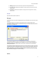
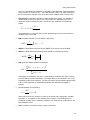
Messages
XLSTAT-PLS uses an innovative message system to give information to the user and to report
problems.
The dialog box below is an example of what happens when an optional selection field
(Quantitative variable(s)) has been activated but left empty. The software detects the problem
and displays the message box.
The information displayed in red (or in blue depending on the severity) to indicate which
object/option/selection is responsible for the message. If you click on back, the dialog box of
the PLS regression will be displayed again and the field corresponding to the Quantitative
variable(s) is activated.
This message should be explicit enough to help you solve the problem by yourself. If a tutorial
is available, the hyperlink "http://www.xlstat.com" links to a tutorial on the subject related to the
problem. Sometimes an email address is displayed below the hyperlink to allow you send an
email to Addinsoft using your usual email software, with the content of the XLSTAT message
being automatically displayed in the email message.
Options
9
XLSTAT-PLS
XLSTAT-PLS offers several options in order to allow you to customize and optimize the use of
the software.
To display the options dialog box of XLSTAT-PLS, click on "Options" in the menu or on the
button of the XLSTAT-PLS toolbar.
: click this button to save the changes you have made.
: click this button to close the dialog box. If you haven’t previously saved the
options, the changes you have made will not be kept.
: click this button to display the help.
: click this button to reload the default options.
General tab:
Language: use this option to change the language of the interface of XLSTAT-PLS.
Dialog box entries:
•
Memorize during one session: activate this option if you want that XLSTAT-PLS
memorizes during one cession (from opening until closing of XLSTAT-PLS) the entries
and options of the dialog boxes.
•
Memorize from one session to the next: activate this option if you want that XLSTATPLS memorizes the entries and options of the dialog boxes from one session to the
next.
− Included for data selections: activate this option so that XLSTAT records the
data selections from one session to the next. This option is useful and saves
your time if you work on spreadsheets that always have the same layout.
Ask for selections confirmation: activate this option so that XLSTAT prompts you to confirm
the data selections once you clicked on the OK button. If you activate this option, you will be
able to verify the number of rows and columns of all the active selections.
Outputs tab:
Position of new sheets: if you choose the "Sheet" option in the dialog boxes of the XLSTAT
functions, use this option to modify the position if the results sheets in the Excel workbook.
Number of decimals: choose the number of decimals to display for the numerical results.
Notice that you always have the possibility to view a different number of decimals afterwards,
by using the Excel formatting options.
Display titles in bold: activate this option so that XLSTAT displays the titles of the results
tables in bold.
10
Using XLSTAT-PLS
Display table headers in bold: activate this option to display the headers of the results tables
in bold.
Display the results list in the report header: activate this option so that XLSTAT displays
the results list at the bottom of the report header.
Display the project name in the report header: activate this option to display the name of
your project in the report header. Then enter the name of your project in the corresponding
field.
Charts tab:
Display charts on separate sheets: activate this option if you want that the charts are
displayed on separate chart sheets. Note: when the charts are displayed on a spreadsheet you
can still transform them into a chart sheet, by clicking the right button of the mouse, and then
selecting "location" and then "As new sheet".
Charts size:
•
Automatic: choose this option if you want that XLSTAT automatically determines the
size of the charts using as a starting value the width and height defined below.
•
User defined: activate this option if you want that XLSTAT displays charts with
dimensions as defined by the following values:
− Width: enter the value in points of the charts width;
− Height: enter the value in points of the charts height.
Display orthonormal charts: activate this option to display orthonormal charts when this is
relevant. Displaying orthonormal allows making sure that there is no distortion effect due to
different scales of the abscissa and ordinates axes that could lead to misinterpretations.
Advanced tab:
Random numbers:
Fix the seed to: activate this option if want to make sure that the computations involving
random numbers always give the same result. Then enter the seed value.
Path for the user's files: this path can be modified if and only if you have administrator rights
on the machine. You can then modify the folder where the user’s files are saved by clicking the
[…] button that will display a box where you can select the appropriate folder. User’s files
include the general options as well as the options and selections of the dialog boxes of the
various XLSTAT functions. The folder where the user’s files are stored must be accessible for
reading and writing to all types of users.
11
PLS/PCR/OLS Regression
Use this module to model and predict the values of one or more dependant quantitative
variables using a linear combination of one or more explanatory quantitative and/or qualitative
variables.
In this section:
Description
Dialog box
Results
Example
References
Description
The three regression methods available in this module have the common characteristic of
generating models that involve linear combines of explanatory variables. The difference
between the three method lies on the way the correlation structures between the variables are
handled.
OLS Regression:
From the three methods it is the most classical. Ordinary Least Squares regression (OLS) is
more commonly named linear regression (simple or multiple depending on the number of
explanatory variables).
In the case of a model with p explanatory variables, the OLS regression model writes
p
Y = β0 + ∑ β j X j + ε
j =1
th
where Y is the dependent variable, β0, is the intercept of the model, Xj corresponds to the j
explanatory variable of the model (j= 1 to p), and ε is the random error with expectation 0 and
variance σ².
In the case where there are n observations, the estimation of the predicted value of the
th
dependent variable Y for the i observation is given by:
p
yˆ i = β 0 + ∑ β j xij
j =1
The OLS method corresponds to minimizing the sum of square differences between the
observed and predicted values. This minimization leads to the following estimators of the
parameters of the model:
13
XLSTAT-PLS
βˆ = ( X ' DX ) −1 X ' Dy
n
1
wi ( yi − yˆ i ) 2
σˆ ² =
∑
∗
W − p i =1
where
β̂ is the vector of the estimators of the β i parameters, X is the matrix of the explanatory
variables preceded by a vector of 1s, y is the vector of the n observed values of the dependent
variable, p* is the number of explanatory variables to which we add 1 if the intercept is not
th
fixed, wi is the weight of the i observation, and W is the sum of the wi weights, and D is a
matrix with the wi weights on its diagonal.
The vector of the predicted values writes:
yˆ = X ( X ' DX ) X ' Dy
−1
The limitations of the OLS regression come from the constraint of the inversion of the X’X
matrix: it is required that the rank of the matrix is p+1, and some numerical problems may arise
if the matrix is not well behaved. XLSTAT-PLS uses algorithms due to Dempster (1969) that
allow circumventing these two issues: if the matrix rank equals q where q is strictly lower than
p+1, some variables are removed from the model, either because they are constant or
because they belong to a block of collinear variables.
Furthermore, an automatic selection of the variables is performed if the user selects a too high
number of variables compared to the number of observations. The theoretical limit is n-1, as
with greater values the X’X matrix becomes non-invertible).
The deleting of some of the variables may however not be optimal: in some cases we might
not add a variable to the model because it is almost collinear to some other variables or to a
block of variables, but it might be that it would be more relevant to remove a variable that is
already in the model and to the new variable.
For that reason, and also in order to handle the cases where there a lot of explanatory
variables, other methods have been developed.
PCR Regression:
PCR (Principal Components Regression) can be divided into three steps: we first run a PCA
(Principal Components Analysis) on the table of the explanatory variables, then we run an OLS
regression on the selected components, the we compute the parameters of the model that
correspond to the input variables.
PCA allows to transform an X table with n observations described by variables into an S table
with n scores described by q components, where q is lower or equal to p and such that (S’S) is
invertible. An additional selection can be applied on the components so that only the r
components that are the most correlated with the Y variable are kept for the OLS regression
step. We then obtain the R table.
The OLS regression is performed on the Y and R tables. In order to circumvent the
interpretation problem with the parameters obtained from the regression, XLSTAT-PLS
transforms the results back into the initial space to obtain the parameters and the confidence
intervals that correspond to the input variables.
14
Using XLSTAT-PLS
PLS Regression:
This method is quick, efficient and optimal for a criterion based on covariances. It is
recommended in cases where the number of variables is high, and where it is likely that the
explanatory variables are correlated.
The idea of PLS regression is to create, starting from a table with n observations described by
p variables, a set of h components with h<p. The method used to build the components differs
from PCA, and presents the advantage of handling missing data. The determination of the
number of components to keep is usually based on a criterion that involves a cross-validation.
The user may also set the number of components to use.
Some programs differentiate PLS1 from PLS2. PLS1 corresponds to the case where there is
only one dependent variable. PLS2 corresponds to the case where there are several
dependent variables. The algorithms used by XLSTAT-PLS are such that the PLS1 is only a
particular case of PLS2.
In the case of the OLS and PCR methods, if models need to be computed for several
dependent variables, the computation of the models is simply a loop on the columns of the
dependent variables table Y. In the case of PLS regression, the covariance structure of Y also
influences the computations.
The equation of the PLS regression model writes:
Y = ThCh' + Eh
= XWh∗Ch' + Eh
(
= XWh Ph'Wh
)
−1
Ch' + Eh
where Y is the matrix of the dependent variables, X is the matrix of the explanatory variables.
Th, Ch, W*h , Wh et Ph, are the matrices generated by the PLS algorithm, and Eh is the matrix of
the residuals.
The matrix B of the regression coefficients of Y on X, with h components generated by the PLS
regression algorithm is given by:
(
B = W h Ph'Wh
)
−1
C h'
Note: the PLS regression leads to a linear model as the OLS and PCR do.
Notes:
1) The three methods give the same results if the number of components obtained from the
PCA (in PCR) or from the PLS regression is equal to the number of explanatory variables.
2) The components obtained from the PLS regression are built so that they explain as well as
possible Y, while the components of the PCR are built to describe X as well as possible.
XLSTAT-PLS allows partly compensating this drawback of the PCR by allowing the
selection of the components that are the most correlated with Y.
15
XLSTAT-PLS
Dialog box
The dialog is divided into several tabs that correspond to a variety of options ranging from the
selection of data to the display of results. You will find below the description of the various
elements of the dialog box.
: click this button to start the computations.
: click this button to close the dialog box without doing any computation.
: click this button to display the help.
: click this button to reload the default options.
: click this button to delete the data selections.
: click these buttons to change the way XLSTAT handles the data. If the arrow points
down, XLSTAT considers that rows correspond to observations and columns to variables. If
the arrow points to the right, XLSTAT considers that rows correspond to variables and columns
to observations.
General tab:
Dependent variable(s): select the dependent variable(s). The data must be numerical. If the
"Variable labels" option is activated make sure that the headers of the variables have also
been selected.
Quantitative variable(s): activate this option if you want to include one or more quantitative
explanatory variables. Then select the corresponding data. The data must be numerical. If the
"Variable labels" option is activated make sure that the headers of the variables have also
been selected.
Qualitative variable(s): activate this option if you want to include one or more qualitative
explanatory variables. Then select the corresponding data. Whatever their Excel format, the
data are considered as categorical. If the "Variable labels" option is activated make sure that
the headers of the variables have also been selected.
Weights: activate this option if you want to weight the observations. If you do not activate this
option, the weights are considered to be equal to 1. The weights must be greater or equal to 0.
If the "Variable labels" option is activated make sure that the header of the selection has also
been selected.
Range: activate this option if you want to display the results starting from a cell in an existing
worksheet. Then select the corresponding cell.
Sheet: activate this option to display the results in a new worksheet of the active workbook.
16
Using XLSTAT-PLS
Workbook: activate this option to display the options in a new workbook.
Variable labels: activate this option if the first row of the data selections (dependent and
explanatory variables, weights, observations labels) includes a header.
Observation labels: activate this option if observations labels are available. Then select the
corresponding data. If the "Variable labels" option is activated you need to include a header in
the selection. If this option is not activated, the observations labels are automatically generated
by XLSTAT-PLS (Obs1, Obs2 …).
Method: choose the regression method you want to use:
•
PLS: activate this option to compute a Partial Least Squares regression.
•
PCR: activate this option to compute Principal Components Regression.
•
OLS: activate this option to compute an Ordinary Least Squares regression.
Options tab:
Common options:
Confidence interval (%): enter the size in % of the confidence interval that is used for the
various tests, parameters and predictions. Default value: 95.
Options for PLS regression:
Stop conditions:
•
Automatic: activate this option so that XLSTAT-PLS automatically determines the
number of components to keep.
•
Qi² threshold: activate this option to fix the threshold value of the Qi² criterion used to
determine if the contribution of a component is significant or not. The default value is
0.0975 which corresponds to 1-0.95².
•
Qi² improvement: activate this option to fix the threshold value of the Qi² improvement
criterion used to determine if the contribution of a component is significant or not. The
default value is 0.05 which corresponds to a 5% improvement. This value is computed
as follows:
Q² ( h ) Imp =
Q ² ( h ) − Q ² ( h − 1)
Q ² ( h − 1)
•
Minimum Press: activate this option so that the number of components used in the
model correspond to the model with the minimum Press statistic.
•
Max components: activate this option to set the pour fixer le maximum number of
components to take into account in the model.
17
XLSTAT-PLS
Options for PCR regression:
Standardized PCA: activate this option to run a PCA on the correlation matrix. Inactivate this
option to run a PCA on the covariance matrix (unstandardized PCA).
Filter components: you may activate one of the two following options to reduce the number of
components used in the model:
•
Min %: activate this option and enter the minimum percentage of total variability that the
selected components should represent.
•
Max number: activate this option to fix the maximum number of components to take
into account.
Sort components by: choose one of the following options to determine "which criterion should
be used to select the components on the basis of the "Min %", or of the "Max Number":
•
Correlations with Ys: activate this option so that the components selection is based on
the sorting down of R² coefficient between the dependent variable Y and the
components. This option is recommended.
•
Eigenvalues: activate this option so that the selection of the components is based on
the sorting down of the eigenvalues corresponding to the components.
Options for PCR and OLS regression:
Intercept: activate this option to fix the intercept (or constant) of the model to a given value.
Then enter the value in the corresponding field (0 by default).
Tolerance: activate this option to allow the OLS algorithm to automatically remove the
variables that would either be constant or highly correlated with other variables or group of
variables (Minimum and default value is 0.0001. Maximum value allowed is 1). The higher the
tolerance, the more the model tolerates collinearities between the variables.
Options for OLS regression:
Constraints: this option is active only if you have selected qualitative explanatory variables.
Choose the type of constraint:
•
a1 = 0: for each qualitative variable, the parameter of the model that corresponds to the
first category of the variable is set to 0. This type of constraint is useful when you
consider that the first category corresponds to a standard, or to a null effect.
•
Sum(ai) = 0: for each qualitative variable, the sum of the parameters corresponding to
the various categories equals 0.
•
Sum(ni.ai) = 0: for each qualitative variable, the sum of the parameters corresponding
to the various categories weighted by their frequency equals 0.
Model selection: activate this option if you want to use one of the following model selection
methods:
•
18
Best model: this method allows choosing the best model among all the models that are
based on a number of variables that is bounded by "Min variables" and "Max variables".
The quality of the model depends on a selection "Criterion".
Using XLSTAT-PLS
20. Criterion: select the criterion in the following list: adjusted R², Mean Squares of
Errors (MSE), Mallows’ Cp, Akaike’s AIC, Schwarz’s SBC, Anemiya’s PC.
21. Min variables: enter the minimum number of variables to take into account in the
model.
22. Max variables: enter the maximum number of variables to take into account in the
model.
Note: this method can lead to very long computations because the total number of
models explored is the sum of the Cn,k where k varies between "Min variables" and
"Max variables", and where Cn,k is n!/[(n-k)!k !]. It is therefore highly recommended that
you increase step by step the value of "Max variables".
•
Stepwise : the selection process starts with the adding of the variable that contributes
the most to the model (the criterion used here is the Student’s t statistic). If a second
variable is such that the probability of its t is lower than the "Threshold level", it is added
to the model. The procedure is the same for the third variable. Then, starting with the
third variable, the algorithm evaluates how the removal of one of the variables would
impact the model. If the probability corresponding to the Student’s t of one of the
variables is greater than the "Threshold level", the variable is removed. The procedure
continues until no variable can be either added or removed from the model.
•
Forward: the procedure is identical to the stepwise, except that there are no removal
steps.
•
Backward: the procedure starts with the selection of all the available variables. The
variables are then removed from the model one by one using the same methodology as
for the stepwise selection.
•
Threshold level: enter the value of the threshold probability for the Student’s t statistic
during the selection process.
Validation tab:
Validation: activate this option if you want to use a sub-sample of the data to validate the
model.
Validation set: choose one of the following options to define how to obtain the observations
used for the validation:
•
Random: the observations are randomly selected. The "Number of observations" N
must then be specified.
•
N last rows: the N last observations are selected for the validation. The "Number of
observations" N must then be specified.
•
N first rows: the N first observations are selected for the validation. The Number of
observations » N must then be specified.
•
Group variable: if you choose this option, you need to select a binary variable with only
0s and 1s. The 1s identify the observations to use for the validation.
Prediction tab:
19
XLSTAT-PLS
Prediction: activate this option if you want to select data to use them in prediction mode. If
activate this option, you need to make sure that the prediction dataset is structured as the
estimation dataset: same variables with the same order in the selections. On the other hand,
variable labels must not be selected: the first row of the selections listed below must
correspond to data.
Quantitative variable(s): activate this option to select the quantitative explanatory variables.
The first row must not include variable labels.
Qualitative Variable(s): activat e this option to select the qualitative explanatory variables. The
first row must not include variable labels.
Observations labels: activate this option if observations labels are available. Then select the
corresponding data. If this option is not activated, the observations labels are automatically
generated by XLSTAT-PLS (PredObs1, PredObs2 …).
Missing data tab:
These options are available only for PCR and OLS regression. With PLS regression, the
missing data are automatically handled by the algorithm.
Remove observations: activate this option to remove the observations with missing data.
Estimate missing data: activate this option to estimate missing data before starting the
computations.
•
Mean or mode : activate this option to estimate missing data by using the mean
(quantitative variables) or the mode (qualitative variables) of the corresponding
variables.
•
Nearest neighbor: activate this option to estimate the missing data of an observation
by searching for the nearest neighbor of the observation.
Outputs tab:
Options common to the three methods:
Descriptive statistics: activate this option to display the descriptive statistics for all the
selected variables.
Correlations: activate this option to display the correlation matrix for the quantitative variables
(dependent and explanatory).
Standardized coefficients: activate this option to display the standardized parameters of the
model (also name beta coefficients).
Equation: activate this option to explicitly display the equation of the model.
Predictions and residuals: activate this option to display the table of predictions and
residuals.
Option for PLS regression:
20
Using XLSTAT-PLS
Bootstrap intervals: activate this option to compute the confidence intervals of the
standardized coefficients. The computations involve a bootstrap method and can therefore
slow down the computations depending on the number of observations. The intervals are
computed using the BC_a intervals suggested in Bastien et al. (2005).
t, u and u~components: activate this option to display the tables corresponding to the
components. If this option is not activated the corresponding charts are not displayed.
c, w, w* and p vectors: activate this option to display the tables corresponding to the vectors
obtained from the PLS algorithm. If this option is not activated the corresponding charts are not
displayed.
VIPs: activate this option to display the table and the charts of the Variable Importance for the
Projection.
Outliers analysis: activate this option to display the table and the charts of the outliers
analysis.
Options for PCR regression:
Factor loadings: activate this option to display the factor loadings. The factor loadings are
equal to the correlations between the principal components and the input variables if the PCA
is based on the correlation matrix (standardized PCA).
Correlations Factors/Variables: activate this option to display the correlations between the
principal component and the input variables.
Factor scores: activate this option to display the factor scores (coordinates of the
observations in the new space) generated by the PCA. The scores are used in the regression
step of the PCR.
Options for PCR and OLS regression:
Analysis of variance: activate this option to display the analysis of variance table.
Adjusted predictions: activate this option to compute and display the adjusted predictions in
the predictions and residuals table.
Cook’s D: activate this option to compute and display the Cook’s distances in the predictions
and residuals table.
Press: activate this option to compute and display the Press statistic.
Charts tab:
Options common to the three methods:
Regression charts: activate this option to display the regression charts:
•
Standardized coefficients: activate this option to display a chart with the standardized
coefficients of the model, and the corresponding confidence intervals.
21
XLSTAT-PLS
•
Predictions and residuals: activate this option to display the following charts:
(1) Regression line: this chart is displayed only if there is one explanatory variable
and if that variable is quantitative.
(2) Explanatory variable versus standardized residuals: this chart is displayed only if
there is one explanatory variable and if that variable is quantitative.
(3) Dependent variable versus standardized residuals.
(4) Predictions versus observed values.
(5) Bar chart of the standardized residuals.
23. Confidence intervals: activate this option to display the confidence intervals on
charts (1) and (4).
Options for the PLS regression and the PCR:
Correlation charts: activate this option to display the charts involving correlations between
components and input variables. In the case of PCR, activate this option to display des
correlation circle.
•
Vectors: activate this option to display the input variables with vectors.
Observations charts: activate this option to display the charts that allow visualizing the
observations in the new space.
•
Labels: activate this option to display the observations labels on the charts. The
number of labels can be modulated using the filtering option.
Biplots: activate this option to display the charts where the input variables and the
observations are simultaneously displayed.
•
Vectors: activate this option to display the input variables with vectors.
•
Labels: activate this option to display the observations labels on the biplots. The
number of labels can be modulated using the filtering option.
Colored labels: activate this option to display the labels with the same color as the
corresponding points. If this option is not activated the labels are displayed in black.
Filter: activate this option to modulate the number of labels displayed:
22
•
Random: the observations to display are randomly selected. The "Number of
observations" N to display must then be specified.
•
N first rows: les N first observations are displayed on the chart. The Number of
observations » N to display must then be specified.
•
N last rows: the N last observations are displayed on the chart. The "Number of
observations" N to display must then be specified.
•
Group variable: if you choose this option, you need to select a binary variable with only
0s and 1s. The 1s identify the observations to display.
Using XLSTAT-PLS
Results
Descriptive statistics: the tables of descriptive statistics display for all the selected variables
a set of basic statistics. For the dependent variables (colored in blue), and the quantitative
explanatory variables, XLSTAT-PLS displays the number of observations, the number of
observations with missing data, the number of observations with no missing data, the mean,
and the unbiased standard deviation. For the qualitative explanatory variables XLSTAT-PLS
displays the name and the frequency of the categories.
Correlation matrix: this table is displayed to allow your visualizing the correlations among the
explanatory variables, among the dependent variables and between both groups.
Results of the PLS regression:
The first table displays the model quality indexes. The quality corresponds here to the
cumulated contribution of the components to the indexes:
•
The Q²cum index measures the global contribution of the h first components to the
predictive quality of the model (and of the sub-models if there are several dependent
variables). The Q²cum(h) index writes:
q
h
Q²cum(h) = 1 − ∏
j =1
∑ PRESS
k =1
q
kj
∑ SCE (
k =1
k j −1)
The index involves the PRESS statistic (that requires a cross-validation), and the Sum
of Squares of Errors (SSE) for a model with one less component. The search for the
maximum of the Q²cum index is equivalent to finding the most stable model.
•
The R²Ycum index is the sum of the coefficients of determination between the
dependent variables and the h first components. It is therefore a measure of the
explanatory power of the h first components for the dependent variables of the model.
•
The R²Xcum index is the sum of the coefficients of determination between the
explanatory variables and the h first components. It is therefore a measure of the
explanatory power of the h first components for the explanatory variables of the model.
A bar chart is displayed to allow the visualization of the evolution of the three indexes when the
number of components increases. While the R²Ycum and R²Xcum indexes necessarily
increase with the number of components, this is not the case with Q²cum.
The next table corresponds to the correlation matrix of the explanatory and dependent
variables with the t and u components. A chart displays the correlations with the t components.
The next table displays the w vectors, followed by the w* vectors and the c vectors, that are
directly involved in the model, as it is shown in the "Description" section. If to h=2 corresponds
a valid model, it is shown that the projection of the x vectors on the y vectors on the variables
23
XLSTAT-PLS
on the w*/c axes chart, gives a fair idea of the sign and the relative weight of the
corresponding coefficients in the model.
The next table displays the scores of the observations in the space of the t components. The
corresponding chart is displayed. If some observations have been selected for the validation,
they are displayed on the chart.
The next table displays the standardized scores of the observations in the space of the t
components. These scores are equivalent to computing the correlations of each observation
(represented by an indicator variable) with the components. This allows displaying the
observations on the correlations map that follows where the Xs, the Ys and the observations
are simultaneously displayed. An example of an an interpretation of this map is available in
Tenenhaus (2003).
The next table corresponds to the scores of the observations in the space of the u and then
the u~ components. The chart based on the u~ is displayed. If some observations have been
selected for the validation, they are displayed on the chart.
The table with the Q² quality indexes allows visualizing how the components contribute to the
explanation of the dependent variables. The table of the cumulated Q² quality indexes allows
measuring the quality that corresponds to a space with an increasing number of dimensions.
The table of the R² and redundancies between the input variables (dependent and
explanatory) and the components t and u~ allow evaluating the explanatory power of the t and
u~. The redundancy between an X table (n rows and p variables) and a c component is the
part of the variance of X explained by c. We define it as the mean of the squares of the
correlation coefficients between the variables and the component:
Rd ( X , c ) =
1 p 2
∑ R (x j , c )
p j =1
From the redundancies one can deduce the VIPs (Variable Importance for the Projection)
that measure the importance of an explanatory variable for the building of the t components.
The VIP for the jth explanatory variable and the component h is defined by:
VIPhj =
h
p
h
∑ Rd (Y ,t )
i =1
∑ Rd (Y , t ) w
i =1
i
2
ij
i
On the VIP charts (one bar chart per component), a border line is plotted to identify the VIPs
that are greater than 0.8: this threshold suggested by Wold (1994) allows identifying the
variables that contribute significantly.
The next table displays the outliers analysis. The DModX (distances from each observation
to the model in the space of the X variables) allow identifing the outliers for the explanatory
explicatives, while the DModY (distances from each observation to the model in the space of
the Y variables) allow identifying the outliers for the dependent variables. On the
corresponding charts the threshold values DCrit are also displayed to help identying of the
outliers: the DMod values that are above the DCrit threshold correspond to outliers. The DCrit
are computed using the threshold values classically used in box plots. The value of the DModX
th
for the i observation writes:
24
Using XLSTAT-PLS
p
DModX i =
n
n − h −1
∑ e( X ,t )
2
ij
j =1
p−h
th
where the e(X,t)ij (i = 1 … n) are the residuals of the regression of X on the j component. The
th
value of the DModY for the i observation writes:
q
DModYi =
∑ e ( Y, t)
j =1
2
ij
q−h
where q is the number of dependent variables and the e(Y,t)ij (i = 1 … n) are the residuals of
th
the regression of Y on the j component.
The next table displays the parameters of the models corresponding to the one or more
dependent variables. It is followed by the equation corresponding to each model, if the number
of explanatory variables does not exceed 20.
For each of the dependent variables a series of tables and charts is displayed.
Goodness of fit statistics: this table displays the goodness of fit statistics of the PLS
regression model for each dependent variable. The definition of the statistics is as follows:
The table of the standardized coefficients (also named beta coefficients) allows comparing
the relative weight of the variables in the model. To compute the confidence intervals, in the
case of PLS regression, the classical formulae based on the normality hypotheses used in
OLS regression do not apply. A bootstrap method suggested by Tenenhaus et al. (2004)
allows estimating the confidence intervals. The greater the absolute value of a coefficient, the
greater the weight of the variable in the model. When the confidence interval around the
standardized coefficients includes 0, which can easily be observed on the chart, the weight of
the variable in the model is not significant.
In the predictions and residuals table, the weight, the observed value of the dependent
variable, the corresponding prediction, the residuals and the confidence intervals are displayed
for each observation. Two types of confidence intervals are displayed: an interval around the
mean (it corresponds to the case where the prediction is made for an infinite number of
observations with a give set of values of the explanatory variables) and an interval around an
individual prediction (it corresponds to the case where the prediction is made for only one
observation). The second interval is always wider than the first one, as the uncertainty is of
course higher. If some observations have been selected for the validation, they are displayed
in this table.
The three charts that are displayed afterwards allow visualizing:
•
the residuals versus the dependent variable,
•
the distance between the predicted and observed values (for an ideal model the all the
points would be on the bisecting line),
•
the bar chart of the residuals.
25
XLSTAT-PLS
If you have selected data to use in prediction mode, a table displays the predictions on the
new observations and the corresponding confidence intervals.
Results of the PCR regression:
The PCR regression requires a Principal Component Analysis step. The first results concern
the latter.
Eigenvalues: the table of the eigenvalues and the corresponding scree plot are displayed.
The number of eigenvalues displayed is equal to the number of non null eigenvalues. If a
components filtering option has been selected it is applied only before the regression step.
If the corresponding outputs options have been activated, XLSTAT-PLS displays the factor
loadings (the coordinates of the input variables in the new space), then the correlations
between the input variables and the components. The correlations are equal to the factor
loadings if the PCA is performed on the correlation matrix. The next table displays the factor
scores (the coordinates of the observations in the new space), and are later used for the
regression step. If some observations have been selected for the validation, they are displayed
in this table. A biplot is displayed if the corresponding option has been activated.
If the filtering option based on the correlations with the dependent variables has been selected,
the components used in the regression step are those that have the greatest determination
coefficients (R²) with the dependent variables. The matrix of the correlation coefficients
between the components and the dependent variables is displayed. The number of
components that are kept depends on the number of eigenvalues and on the selected options
("% Min" or "Max components").
If the filtering option based on the eigenvalues has been selected, the components used in the
regression step are those that have the greatest eigenvalues. The number of components that
are kept depends on the number of eigenvalues and on the selected options ("% Min" or "Max
components").
Results common to the PCR et OLS regressions:
Goodness of fit statistics: this table displays statistics that are related to the goodness of fit
of the regression model:
•
Observations: the number of observations taken into account for the computations. In
the formulae below, n corresponds to number of observations.
•
Sum of weights: the sum of weights of the observations taken into account. In the
formulae below, W corresponds to the sum of weights.
•
DF: the number of degrees of freedom of the selected model (corresponds to the error
DF of the analysis of variance table).
•
R²: the coefficient of determination of the model. This coefficient, which value is
between 0 and 1, is displayed only if the intercept of the model has not been fixed by
the user. The value of this coefficient is computed as follows:
n
R² = 1 −
∑w ( y
i =1
n
i
∑w(y
i =1
26
i
i
i
− yˆi )
2
, with
− y )2
y=
1 n
∑ wi yi
n i=1
Using XLSTAT-PLS
The R² is interpreted is the proportion of variability of the dependent variable explained
by the model. The close the R² to 1, the better fitted the model. The major drawback of
the R² is that it does not take into account the number variables used to fit the model.
•
Adjusted R²: the adjusted coefficient of determination of the model. The adjusted R²
can be negative if the R² is close to zero. This coefficient is displayed only if of the
model has not been fixed by the user. The value of this coefficient is computed as
follows:
R̂² = 1 − (1 − R ² )
W −1
W − p −1
The adjusted R² is a correction of the R² that allows taking into account the number of
variables used in the model.
•
MSE: the Mean Squares of Errors (MSE) is defined by:
MSE =
n
1
2
wi ( yi − yˆi )
∑
W − p * i=1
•
RMSE: the Root Mean Squares of Errors (RMSE) is the square root of the MSE.
•
MAPE: the Mean Absolute Percentage Error (MAPE) is computed as follows:
MAPE =
•
100 n
y − yˆ i
wi i
∑
W i=1
yi
DW: the Durbin-Watson statistic is defined by
n
DW =
∑ ( y
i= 2
i
− yˆ i ) − ( yi −1 − yˆi −1 )
n
∑w ( y
i =1
i
i
2
− yˆi )
2
This statistic corresponds to the order 1 autocorrelation coefficient and allows verifying
if the residuals are not autocorrelated. The independence of the residuals is one of the
hypotheses of the linear regression. The user will need to look at a Durbin-Watson table
to know if the hypothesis of independence between the residuals is accepted or
rejected.
•
Cp: the Mallows’ Cp is defined by :
Cp =
SCE
+ 2 p * −W
σˆ
where SSE is the sum of squares of errors for the model with p explanatory variables,
and where σ̂ corresponds to the estimator of the variance of the residuals for the
model that includes all the explanatory variables. The closer the Cp coefficient to p* the
less biased the model.
•
AIC: the Akaike’s Information Criterion (AIC) is defined by:
27
XLSTAT-PLS
SCE
AIC = W ln
+ 2p *
W
This criterion suggested by Akaike (1973) derives from the information theory and is
based on the Kullback and Leibler measure (1951). It is a models selection criterion that
penalizes models for which the addition of a new explanatory variable does not bring
sufficient information. The lower the AIC, the better the model.
•
SBC: the Schwarz’s Bayesian Criterion writes:
SCE
SBC = W ln
+ ln (W ) p *
W
This criterion suggested by Schwarz (1978) is close to the AIC, and the goal is to
minimize it.
•
PC: the Anemiya’s Prediction Criterion) writes
PC =
(1 − R² )( W + p *)
W − p*
This criterion suggested by Anemiya (1980) allows as the adjusted R² to take into
account the parsimony of the model.
•
Press RMCE: la Press RMSE statistic is displayed only if the corresponding option has
been activated in the dialog box. The Press statistic is defined by
Press = ∑ wi ( yi − yˆ i (− i) )
n
2
i =1
where
yˆ i( − i) is the prediction of the ith observation when it is not included in the data
set used for the estimation of the parameters of the model. When obtain:
Press RMCE =
Press
W - p*
The Press RMSE can then be compared to the RMSE. A large difference between
both indicates that the model is sensitive to the presence or absence of some
observations.
The analysis of variance table allows evaluating how much information the explanatory
variables bring to the model. In the case where the intercept of the model is not fixed by the
user, the explanatory power is measured by comparing the fit of the selected model with the fit
of a basic model where the dependent variable equals its mean. When the intercept is fixed to
a given value, the selected model is compared to a basic model where the dependent model
equals the fixed intercept.
In the case of a PCR regression, the first table of model parameters corresponds to the
parameters of the model based on the selected components. This table is not easy to interpret.
For that reason a transformation is performed to obtain the parameters of the model
corresponding to the input variables. The latter table is directly obtained in the case of an OLS
regression. In this table you will find the estimate of the parameters, the corresponding
28
Using XLSTAT-PLS
standard error, the Student’s t, the corresponding probability, as well as the confidence
interval.
The equation of the model is then displayed to facilitate the visualization or the reuse of the
model.
The table of the standardized coefficients (also named beta coefficients) allows comparing
the relative weight of the variables in the model. The greater the absolute value of a coefficient,
the greater the weight of the variable in the model. When the confidence interval around the
standardized coefficients includes 0, which can easily be observed on the chart, the weight of
the variable in the model is not significant.
In the predictions and residuals table, the weight, the value of the explanatory variable if
there is only one, the observed value of the dependent variable, the corresponding prediction,
the residuals and the confidence intervals, the adjusted prediction and the Cook’s D, are
displayed for each observation. Two types of confidence intervals are displayed: an interval
around the mean (it corresponds to the case where the prediction is made for an infinite
number of observations with a give set of values of the explanatory variables) and an interval
around an individual prediction (it corresponds to the case where the prediction is made for
only one observation). The second interval is always wider than the first one, as the
uncertainty is of course higher. If some observations have been selected for the validation,
they are displayed in this table.
The charts that follow allow visualizing the results listed above. If there is only one explanatory
variable in the model, and if that variable is quantitative, then the first chart allows visualizing
the observations, the regression line and the confidence intervals around the prediction. The
second chart displays the standardized residuals versus the explanatory variable. The
residuals should be randomly distributed around the abscissa axis. If a trend can be observed,
that means there is a problem with the model.
The three charts that are displayed afterwards allow visualizing respectively the standardized
residuals versus the dependent variable, the distance between the predicted and observed
values (for an ideal model the all the points would be on the bisecting line), and the bar chart of
the standardized residuals. The third chart makes it possible to quickly see if there is an
unexpected number of high residuals: the normality assumption for the residuals is such that
only 5% of the standardized residuals should be out of the ]-2, 2[ interval.
If you have selected data to use in prediction mode, a table displays the predictions on the
new observations and the corresponding confidence intervals.
OLS regression results:
If the Type I SS and Type III SS (SS: Sum of Squares) options have been activated, the
corresponding tables are displayed.
The Type I SS table allows visualizing the influence of the progressive addition of new
explanatory variables to the model. The influence is given by the Sum of Squares of Errors
(SSE), de la Mean Squares of Errors (MSE), the Fisher’s F statistic, and the probability
corresponding to the Fisher’s F. The smaller the probability, the more information the variable
brings to the model. Note: the order of selection of the variables influences the results obtained
here.
The Type III SS table allows visualizing the influence of the withdrawal of an explanatory
variable on the goodness of fit of the model, all the other variables being included. The
influence is measured by the Sum of Squares of Errors (SSE), de la Mean Squares of Errors
(MSE), the Fisher’s F statistic, and the probability corresponding to the Fisher’s F. The smaller
29
XLSTAT-PLS
the probability, the more information the variable brings to the model. Note: the order of the
variables in the selection does not influence the results in this table.
Examples
Tutorials on how to use XLSTAT-PLS are available on the Addinsoft website on following
pages:
http://www.xlstat.com/demo-pls.htm
http://www.xlstat.com/demo-pcr.htm
References
Akaike H. (1973). Information Theory and the Extension of the Maximum Likelihood Principle,
Second International Symposium on Information Theory, V.N. Petrov and F. Csaki, Budapest:
Akailseoniai-Kiudo, pp 267 -281.
Anemiya T. (1980). Selection of Regressors. International Economic Review, 21, pp 331-354.
Bastien P., Esposito Vinzi V. and Tenenhaus M. (2005). PLS Generalised Regression.
Computational Statistics and Data Analysis, 48, pp 17-46.
Dempster A.P. (1969). Elements of Continuous Multivariate Analysis. Addison-Wesley, Reading,
MA.
Kullback S. and Leibler R. A. (1951). On information and sufficiency. Annals of Mathematical
Statistics, 22, pp 79-86.
Schwarz G. (1978). Estimating the Dimension of a Model," Annals of Statistics, 6, pp 461-464.
Tenenhaus M. (1998). La Régression PLS, Théorie et Pratique. Technip, Paris.
Tenenhaus, M., Pagès, J., Ambroisine L. and & Guinot, C. (2005). PLS methodology for
studying relationships between hedonic judgements and product characteristics. Food Quality
an Preference. 16, 4, pp 315-325.
Wold S. (1995). PLS for multivariate linear modelling. In: van de Waterbeemd H, ed. QSAR:
Chemometric Methods in Molecular Design. Vol 2. Weinheim, Germany. Wiley-VCH pp 195218.
30