1
Windows QTL Cartographer 2.5
User Manual
© 2010 N.C. State University, Bioinformatics Research Center
I
Windows QTL Cartographer 2.5
Table of Contents
About Windows QTL Cartographer
1
WinQTLCart
...................................................................................................................................
features
1
Compatible
...................................................................................................................................
programs and formats
1
System...................................................................................................................................
requirements
2
Installing,
...................................................................................................................................
uninstalling, upgrading
2
Using WinQTL - a high-level overview
2
When to
...................................................................................................................................
use WinQTLCart
4
WinQTLCart Windows & Menus
4
Main window
...................................................................................................................................
- Menus
4
Main w indow
Main w indow
Main w indow
Main w indow
Main w indow
Main w indow
- ..........................................................................................................................................................
Menus - File
4
- ..........................................................................................................................................................
Menus - Edit
5
- ..........................................................................................................................................................
Menus - View
5
- ..........................................................................................................................................................
Menus - Method
5
- ..........................................................................................................................................................
Menus - Tools
6
- ..........................................................................................................................................................
Menus - Help
7
Chromosome
...................................................................................................................................
graph display - Menus
7
Chrom osom e ..........................................................................................................................................................
graph - Menus - File
7
Chrom osom e graph
..........................................................................................................................................................
- Menus - View
7
Chrom osom e graph
..........................................................................................................................................................
- Menus - Setting
8
Main window
...................................................................................................................................
tour
9
Main w indow ..........................................................................................................................................................
- Tree Pane
10
Main w indow ..........................................................................................................................................................
- Form Pane
12
Main w indow ..........................................................................................................................................................
- Data Pane
12
Graph...................................................................................................................................
window - Menus
12
Graph w indow..........................................................................................................................................................
- Menus - File
13
Graph w indow..........................................................................................................................................................
- Menus - Chrom
13
Graph w indow..........................................................................................................................................................
- Menus - Traits
14
Graph w indow..........................................................................................................................................................
- Menus - Effects
14
Graph w indow..........................................................................................................................................................
- Menus - Tools
15
Graph w indow..........................................................................................................................................................
- Menus - Setting
15
One-page
...................................................................................................................................
display window - Menus
16
One-Page w indow
..........................................................................................................................................................
- Menus - File
16
One-Page w indow
..........................................................................................................................................................
- Menus - View
16
One-Page w indow
..........................................................................................................................................................
- Menus - Setting
17
Graph...................................................................................................................................
window - Procedures
17
Tracing coordinates
..........................................................................................................................................................
on the graph
19
Selecting traits
..........................................................................................................................................................
for graph display
20
Selecting chrom
..........................................................................................................................................................
osom es for graph display
21
Setting display
..........................................................................................................................................................
param eters
21
Setting a test ..........................................................................................................................................................
hypothesis
23
Show ing QTL ..........................................................................................................................................................
inform ation
24
© 2010 N.C. State University, Bioinformatics Research Center
Contents
WinQTLCart Procedures
II
25
Setting
...................................................................................................................................
the working directory
25
Importing
...................................................................................................................................
and exporting
25
Im porting files
.......................................................................................................................................................... 25
Exporting source
..........................................................................................................................................................
data and results
29
Exporting source
.........................................................................................................................................................
data to QTL Cartographer
30
Exporting source
.........................................................................................................................................................
data to an MCD file
30
Exporting results
.........................................................................................................................................................
from the Graph w indow
31
Working
...................................................................................................................................
with source data files
31
Opening source
..........................................................................................................................................................
data files
32
Working w ith ..........................................................................................................................................................
a source file's m arker genotype data
32
Working w ith ..........................................................................................................................................................
a source file's traits values
33
Working w ith ..........................................................................................................................................................
a source file's basic inform ation
34
Working w ith ..........................................................................................................................................................
source file's individual inform ation
35
Working w ith ..........................................................................................................................................................
source file's chrom osom e inform ation
37
Working w ith ..........................................................................................................................................................
source file's trait inform ation
38
Working w ith ..........................................................................................................................................................
source file's other trait inform ation
39
MCD file form..........................................................................................................................................................
at
39
Creating
...................................................................................................................................
a new source data file from raw data
44
Creating
...................................................................................................................................
simulation data
51
Single-marker
...................................................................................................................................
analysis
55
Setting
...................................................................................................................................
threshold levels (IM & CIM)
56
Setting threshold
..........................................................................................................................................................
levels m anually
57
Setting threshold
..........................................................................................................................................................
levels via perm utations
57
Interval
...................................................................................................................................
Mapping
58
Running interval
..........................................................................................................................................................
m apping analysis
58
Composite
...................................................................................................................................
Interval Mapping
60
Running com posite
..........................................................................................................................................................
interval m apping analysis
60
Multiple
...................................................................................................................................
Interval Mapping
63
About the MIM..........................................................................................................................................................
form
63
Creating MIM ..........................................................................................................................................................
initial m odel
65
Regression.........................................................................................................................................................
options
66
CIM search.........................................................................................................................................................
option
68
MIM search.........................................................................................................................................................
option
69
Refining the MIM
..........................................................................................................................................................
m odel
70
Multiple-trait
...................................................................................................................................
MIM
72
About the Mt-MIM
..........................................................................................................................................................
form
72
Mt-MIM Control
..........................................................................................................................................................
File
74
Mt-MIM Functions
.......................................................................................................................................................... 75
Bayesian
...................................................................................................................................
Interval Mapping
76
Running Bayesian
..........................................................................................................................................................
interval m apping analysis
77
Multiple-trait
...................................................................................................................................
analysis
78
Drawing
...................................................................................................................................
a chromosome tree
78
Adding QTL positions
..........................................................................................................................................................
to the chrom osom e graphics
80
Tutorials
81
Import...................................................................................................................................
data files
81
© 2010 N.C. State University, Bioinformatics Research Center
II
III
Windows QTL Cartographer 2.5
Im port data - INP
..........................................................................................................................................................
form at
81
Using Em ap function
.......................................................................................................................................................... 81
Im port data - OUT
..........................................................................................................................................................
form at
81
Im port data - MapMaker
..........................................................................................................................................................
form at
82
Im port data - Excel
..........................................................................................................................................................
form at
82
Im port data - CSV
..........................................................................................................................................................
form at
82
Simulation
...................................................................................................................................
source data file
82
Create...................................................................................................................................
new source data file
83
Single...................................................................................................................................
marker analysis
83
Interval
...................................................................................................................................
mapping
84
Composite
...................................................................................................................................
interval mapping
84
Multiple-trait
...................................................................................................................................
analysis
84
Multiple
...................................................................................................................................
Interval Mapping
84
Bayesian
...................................................................................................................................
interval mapping
85
Result...................................................................................................................................
manipulation
85
Technical notes
85
Troubleshooting
................................................................................................................................... 85
1. Errors even..........................................................................................................................................................
to run Single Marker Analysis
85
2. Why m y trait
..........................................................................................................................................................
values are truncated into integers
86
3. WinQTLCart..........................................................................................................................................................
cannot im port Map inform ation from selected file
86
4. Invalid file or
..........................................................................................................................................................
w rong form at m essages
86
5. Failures w hen
..........................................................................................................................................................
I try to creat MCD file from text files
86
Technical
...................................................................................................................................
Support
86
Credits
...................................................................................................................................
& acknowledgements
87
Index
88
© 2010 N.C. State University, Bioinformatics Research Center
About Windows QTL Cartographer
1
About Windows QTL Cartographer
WinQTLCart features
Windows QTL Cartographer maps quantitative trait loci (QTL) in cross populations from inbred lines.
WinQTLCart includes a powerful graphic tool for presenting mapping results and can import and export
data in a variety of formats.
WinQTLCart incorporates many of the modules found in its command-line sibling, QTL Cartographer, and
provides a graphical interface to many of QTL Cartographer's features.
WinQTLCart implements the following statistical methods:
Single-marker analysis 55
Interval mapping 58
Composite interval mapping 60
Bayesian interval mapping 76
Multiple interval mapping 63
Multiple trait analysis 78
Multiple trait MIM analysis 78
Features
Supports various QTL mapping methods
View, copy, and print graphs
Includes an interface to help you build a source data file that WinQTLCart can use for analysis
Import 25 data from Mapmaker / QTL and Microsoft Excel and CSV formats
Export 29 graph data to Windows Excel format
View, copy, and print chromosome information 78 graphically
Produce a simulation 51 data file
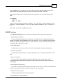
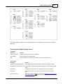
Compatible programs and formats
WinQTLCart can import and export data files in a variety of formats.
Import success depends on the data file's format. Some data may need to be formatted manually before
WinQTLCart can import it.
Applications
Formats Supported
MapMaker/QTL
.MAP – Map file
.MPS – Map file
.RAW – Cross data file
X
Microsoft Excel
.XLS
X
Microsoft CSV
.CSV
X
QTL Cartographer
.INP – Map and Cross data files
.MAP – Map file
.CRO – Cross data file
X
X
WinQTLCart
.MCD – Source data file
X
X
© 2010 N.C. State University, Bioinformatics Research Center
Import
Export
X
2
Windows QTL Cartographer 2.5
Related topics
Creating a new source data file 44
Troubleshooting import errors 86
Importing files 25
Exporting source data and results
29
System requirements
WinQTLCart can run on the following operating systems: Windows 95, 98, ME, NT, 2000, XP and
Windows 7.
Because some WinQTLCart windows are quite large, the suggested minimum monitor resolution is
1024x768.
20MB free disk space for program files.
512MB RAM.
Any mouse or pointing device supported by Windows.
Installing, uninstalling, upgrading
Installing
To install, double-click the WQTLSetup.exe file and follow the prompts. The default install directory is C:
\NCSU\WinQTLCart2.5, though you can specify a different directory.
The installer places a shortcut to the Windows QTL Cartographer program on your PC's Desktop,
labeled WinQTLCart. Double-click the icon to run the program.
Uninstalling
To uninstall, run the Add/Remove Programs control panel and select Windows QTL Cartographer from
the installed programs list.
Upgrading
If you have a prior version of WinQTLCart already on your PC, simply run the installer program.
Upgrading to a new version of WinQTLCart does not overwrite your working files. However, the upgrade
will replace the sample files that are part of the WinQTLCart distribution.
Note
You should close current running version of WinQTLCart first before installing the upgrading version.
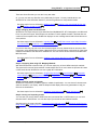
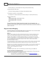
Using WinQTL - a high-level overview
Your goals in using WinQTLCart may include preparing data for publication or continued research into
possible QTL sites.
Step 1—Preparing your source data
Your data files may come from another program or they may exist as raw data files. For WinQTLCart to
work with your files, they need to conform to the program's .MCD file format 39 . Review that file, as well
as the other files included in the WinQTLCart distribution, such as the .QRT, .QPE, and other files.
© 2010 N.C. State University, Bioinformatics Research Center
Using WinQTL - a high-level overview
3
These are all text files that you can view in any text editor.
Or, you may not have any data files or any data ready for import. You may instead want to use
WinQTLCart to create simulation data to try out some hypotheses to view potential results.
See these topics for more information: MCD file format
data 44 , Creating simulation data 51
39
, Creating a new source data file from raw
Step 2—Bringing data into WinQTLCart
WinQTLCart can import map and cross data files from MapMaker/QTL, QTL Cartographer, and Microsoft
Excel. As part of the import, WinQTLCart runs verification checks against the data. If the data does not
conform to the accepted format, WinQTLCart displays an error message that should indicate the source
of the problem.
See these topics for more information: Importing files 25 , WinQTLCart cannot import Map information
from selected file 86 , Invalid file or wrong format messages 86
Your source data may not have come from another program, but may instead exist as raw source files.
In that case, using WinQTLCart's Create a New Source File command steps you through all of the steps
needed to translate the raw data into a readable form. The new source file will conform to WinQTLCart's
MCD file format.
See these topics for more information: Creating a new source data file from raw data
format 39
44
, MCD file
Step 3—Analyzing data using QTL Mapping Methods
With WinQTLCart able to view the data, you can then select any of seven different analysis methods.
The end result for some of these methods is another MCD file, but in most cases the process will create
a .QRT result file that WinQTLCart can use to graph QTL information.
See these topics for more information: Single-marker analysis 55 , Interval Mapping 58 , Composite
Interval Mapping 60 , Multiple Interval Mapping 63 , Bayesian Interval Mapping 76 , Multiple-trait
Analysis 63 , Multiple-trait MIM.
Step 4—Viewing results and graphs
WinQTLCart can present your data in graphics suitable for publication. You can show all chromosomes
and their intervals in one display, while the Graph window display offers many parameters to help you
fine-tune the visualization.
See these topics for more information: Drawing a chromosome tree
78
, Graph Window tour
17
Step 5—Saving and exporting results
You can save your source data in .MCD format and your results files in .QRT format so you can work
with them later in WinQTLCart. You can also export your results to other selected formats.
See these topics for more information: Exporting source data and results 29 , Exporting results from the
Graph window 31 , Exporting source data to an MCD file 30 , Exporting source data to QTL Cartographer
30
© 2010 N.C. State University, Bioinformatics Research Center
4
Windows QTL Cartographer 2.5
When to use WinQTLCart
You can use WinQTLCart for any kind of data that is cross populations from inbred lines. WinQTLCart is
a particularly powerful tool when you want to explore your results graphically.
Prior to doing experiments, you could use WinQTLCart to explore some "what-if" scenarios in planning
your experimental design. In WinQTLCart, you can create simulation data and then vary parameters
setting to explore various QTL models.
However, if you're working on a repetitive task that would be better off scripted, you may want to turn to
QTL Cartographer, WinQTLCart's command-line sibling. For example, if you have expression data with
thousands of features, you might want to run interval mapping on each feature, which would take a long
time. This task can be automated via a shell script and made to run overnight. The results can then be
imported into WinQTLCart and its graphs charted.
WinQTLCart Windows & Menus
Main window - Menus
Menus in Main window include File
4
, Edit
5
, View
5
, Method
5
, Tools
6
, and Help
7
.
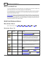
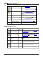
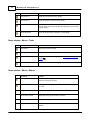
Main window - Menus - File
Icon
Command
Shortcut Key Function
New...
Ctrl + N
Create a new source data file from raw text files.
See Creating a new source data file 44
Open...
Ctrl + O
Open a data file, result file or text file.
Source data files you can open in WinQTLCart have the .
MCD extension. Results files have the .QRT extension.
Files with any other extension are opened as text files.
Close
Close the currently selected file. (The currently selected .
MCD file's name is in the title bar and highlighted in the
Tree pane).
Save As...
Save the currently active source data to a file with mcd
format or a file with Microsoft Excel format.
Import...
Ctrl + I
Import files in a variety of formats. See the importing files
25 topic
Simulation...
Opens the Simulate Data dialog. See creating a
simulation data file 51
Export...
Export the selected file to a different format. See Exporting
source data and results 29
© 2010 N.C. State University, Bioinformatics Research Center
WinQTLCart Windows & Menus
Print...
Ctrl + P
5
Print the selected file in data pane.
Print Setup...
Opens Windows' Print Setup dialog box.
Recently used
files
WinQTLCart displays the last 6 data files you've worked
with.
Exit
Closes WinQTLCart.
If you have unsaved data, you'll be prompted to save it.
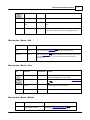
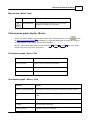
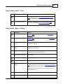
Main window - Menus - Edit
Command
Shortcut Key Function
Copy
Ctrl + C
Copy selected text in Data pane
Select All
Ctrl + A
Click in the Data pane 12 and then choose this command to select all text
in the data pane. Enables you to easily select and copy the text to a
separate file.
12
to the Windows clipboard.
Main window - Menus - View
Icon
Command
Shortcut Key Function
Data Summary
Result Graph...
Summarizes statistical information of active source
data file and displays in Text window.
Ctrl + G
View result file in the Graph window. See Graph Window
tour 17
Toolbar
Select to toggle the Toolbar display.
Status bar
Select to toggle the Status bar display.
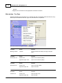
Main window - Menus - Method
Icon
Command
Function
Single Marker Analysis...
Displays the Single Marker Analysis
© 2010 N.C. State University, Bioinformatics Research Center
55
form.
6
Windows QTL Cartographer 2.5
Interval Mapping...
Displays the Interval Mapping
Composite Interval Mapping...
Displays the Composite Interval Mapping form
Multiple Interval Mapping...
Displays the Multiple Interval Mapping 63 form.
Click "OK" button to start MIM analysis and click
"MtMIM" button to choose multiple-trait MIM
analysis.
Multiple Trait MIM Analysis...
Display the Multiple Trait MIM Analysis form.
58
form.
Multiple Traits IM-CIM Analysis... Displays the Multiple Trait Analysis
78
60
.
form.
Category Trait Analysis...
Displays the Category Trait Analysis form.
Bayesian Interval Mapping...
Displays the Bayesian Interval Mapping
eQTL MIM Analysis...
Displays the eQTL MIM Analysis form.
76
form.
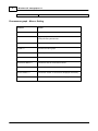
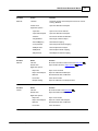
Main window - Menus - Tools
Icon
Command
Shortcut
Key
Function
Set Working directory...
Set the default working directory. See Setting the
working directory 25
Draw chromosome graph...
Show and print graphic displays of chromosomes
from the Current active .MCD file. See Drawing a
chromosome tree 78
Copy between trait and
otrait...
Copy normal trait to Other trait (category trait) or vise
verse.
Delete markers of same
position...
Delete markers that have the same position in a
chromosome and only keep one marker.
Notepad...
Ctrl + Shift + Opens Notepad. Use Notepad as a convenient text
N
editor to help format source data files.
Calculator...
Ctrl + Shift + Open the Windows Calculator accessory.
C
© 2010 N.C. State University, Bioinformatics Research Center
WinQTLCart Windows & Menus
7
Main window - Menus - Help
Icon
Command
Function
About WinQTLCart
Display About dialog of WinQTLCart. You can open
WinQTLCart upgrade site in this dialog.
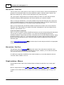
Chromosome graph display - Menus
Open a mcd source data file. From the Main window, select Tools>DrawChrom or click
to draw
the trees of chromosome graph 78 and markers in a single large window that is suitable for copying to
an image program for later editing or printing and publication.
Menus in Chromosome graph display window include File
that will Copy content in window to the clipboard.
7
, View
7
, Setting
8
, and Copy_Graph
Chromosome graph - Menus - File
Command
Function
Copy to Clipboard
Copies content in window to the clipboard.
Print Graph…
Print the graph.
Exit
Close the window and return to the Main window.
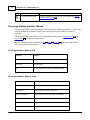
Chromosome graph - Menus - View
Command
Function
Proportion of Marker Number
Show length of chromosome graph in proportion of marker number
Proportion of Chromosome
Len
Show length of chromosome graph in proportion of chromosome length
in cM
Next Page >>
Show next page of the graph if there are multiple pages.
First Page
Show First page of the graph.
Add QTL Positions...
Display QTL positions in the graph.
© 2010 N.C. State University, Bioinformatics Research Center
8
Windows QTL Cartographer 2.5
Chromosome graph - Menus - Setting
Command
Function
Select Chromosomes
Select chromosomes to be showed in graph.
Show Chromosome Name
Toggle display between chromosome names or chromosome
labels produced by WinQTLCart.
Font Size >>
Increase font size of graph.
Font Size <<
Decrease font size of graph.
Space Between >>
Increase space between chromosomes.
Space Between <<
Decrease space between chromosomes.
Chromosome Name >>
Increase font size of chromosome names.
Chromosome Name <<
Decrease font size of chromosome names.
Column Number >>
Increase the number of chromosome displayed horizontally.
Column Number <<
Decrease the number of chromosome displayed horizontally.
© 2010 N.C. State University, Bioinformatics Research Center
WinQTLCart Windows & Menus
9
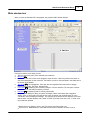
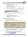
Main window tour
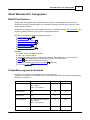
When you start up Windows QTL cartographer, the program's Main window displays.
From top to bottom, here's what you see:
1. Title bar. Shows the name of the selected source data file.
2. Menu bar 4 .
3. Toolbar with one-click access to the program's major functions. Hover the pointer over a button to
see a brief description of that command. The button's function is also described in the Status bar at
the bottom of the window.
4. Tree pane 10 for file management. Lists open files and organizes files under various category
names (Source Files, Text Files, Results Files).
5. Form pane 12 for displaying and controlling analysis of source data files. The form pane contents
change based on the analysis method you select.
6. Data pane 12 for displaying data of currently selected file.
7. The Status bar displays a variety of system messages; select View>Status bar to toggle its
display. Click on each node in the tree pane or hover the pointer over a toolbar button or menu
command to see the displayed message. The right area of the status bar also displays the current
date and time, and also displays CAP, NUM, or SCRL if the Caps Lock, Num Lock, or Scroll Lock
keys have been pressed.
Double-click on a category name in the Tree pane to open files of that type.
Left-click on a .MCD filename to make that the active source data file on which to run an
© 2010 N.C. State University, Bioinformatics Research Center
10
Windows QTL Cartographer 2.5
analysis.
Right-click on a filename to see appropriate commands for that file.
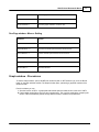
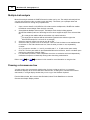
Main window - Tree Pane
The Main Window's Tree pane allows you to manage open files. The following table describes the many
different options available via left-click, right-click, and double-click operations.
Source file selected with right-click options displayed
Tree Item
Action
Function
Message window
Left-click
Displays WinQTLCart startup message in the data
pane.
Tree Item
Action
Function
Source files root
Double-click
Open a source data file (.MCD)
Right-click>Open a File
Open a source data file (.MCD)
Tree Item
Action
Function
Result files root
Double-click
Open a result file (.QRT)
Right-click>Open File
Open a result file
Tree Item
Action
Function
Text files root
Double-click
Open a text file (.TXT).
Right-click>Open File
Open a text file
© 2010 N.C. State University, Bioinformatics Research Center
WinQTLCart Windows & Menus
11
Tree Item
Action
Function
.MCD file
Left-click
Show file contents in the Data pane and set as current
working .MCD file
Double-click
Open the .MCD file in Notepad
Right-click options…
>Open File
Open a new source data file
>Open with Notepad
Open the .MCD file in Notepad
>Refresh
Re-load the file after modification
>Single Marker
Start single marker analysis
>Interval Mapping
Start interval mapping
>Composite IM
Start composite interval mapping
>Multiple Traits
Start multiple traits analysis
>Multiple IM
Start multiple interval mapping
>Bayesian IM
Start Bayesian interval mapping
Tree Item
Action
Function
.QRT file
Left-click
Show this result file in text format via the Data pane
Double-click
Open the QRT file in the Graph window
Right-click options…
>Open File
Open a new result file
>Open with Notepad
Open the .QRT file with Notepad
>Refresh
Re-load the file after modification
>Close File
Close the result file
>Graphic Dialog
Open the .QRT file in the Graph window
Tree Item
Action
Function
.TXT file
Left-click
Show this text file in the Data pane
Double-click
Open the text file with Notepad
Right-click options…
>Open File
Open a new text file
>Open with Notepad
Open the .TXT file with Notepad
>Refresh
Re-load the file after modification
>Close File
Close the text file.
© 2010 N.C. State University, Bioinformatics Research Center
12
17
12
.
12
Windows QTL Cartographer 2.5
Main window - Form Pane
The Form pane is the control panel you use to analyze your source data. It serves as a dashboard that
presents a lot of information about your source data file at a glance. (The Form pane is keyed to the .
MCD source data file only; it does not show information for any other file format.)
This "control panel" changes based on the analysis method you select. For each analysis method,
WinQTLCart displays different parameters and controls that help you control the analysis.
When you first open WinQTLCart, you see the standard Source Data File Information form. Most of the
options are disabled because no source data file has been loaded. Select an analysis method from the
drop down list in the Analysis box on the right to begin working with the data.
When you have opened a file, WinQTLCart enables the buttons and controls on the Source Data File
Information form. These enable you to perform some basic manipulations to the source data (such as
add traits, map information, etc.)
Forms and disabled commands
When you select an analysis method, WinQTLCart assumes you want to keep working with that method
until you save your data or cancel the analysis. If you select the Interval Mapping (IM) method,
WinQTLCart disables several toolbar and menu commands (such as the other analysis methods, setting
the working directory, and so on). You need to either save your data or press the Cancel button on the
IM form to leave the IM analysis mode. Leaving an analysis method re-displays the Source Data File
Information pane.
See the Source data file information 31 topic and the topics for each analysis method for the appropriate
screen shot relevant to that method.
Main window - Data Pane
The large pane under the Form pane 12 displays the content of the active data or results file in text
format. You cannot edit the displayed information from this pane. However, you can select the text with
your cursor and copy the selected text to the clipboard.
For .MCD source data files, WinQTLCart color-codes the data so you can easily determine what are
comments, labels, headers, and so on.
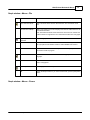
Graph window - Menus
From the Main window, select View>Visualize Result to display the result file (*.qrt) in result graph
window.
Menus in Graph window include File
13
, Chrom
13
, Traits
14
, Effects
14
, Tools
15
, and Setting
15
.
In addition to the toolbar and menu commands, some functions are available by right-clicking on the
graph.
© 2010 N.C. State University, Bioinformatics Research Center
WinQTLCart Windows & Menus
13
Graph window - Menus - File
Command
Function
Open QTL Result File...
Open a result file. Files with the .QRT extension are considered result
files.
Add QTL Result Graph...
Adds a new graph to the current display. Files with the .QRT extension are
considered result files.
Note: The added result file should have same chromosome number and
marker number as original one. You could add more than one new graph.
Copy Graphic to
Clipboard
Copies the graph to the Windows clipboard.
Save As New Name...
Save the file under a different name in .QRT format. You may want to do
this if you plan to work with the results in a later WinQTLCart session.
Save As Text File...
Save the results as a text file. You may want to do this if you plan to use
the text file in another program.
Save As Excel File...
Save the data as an Excel file. Use Excel's charting capabilities to draw
the graph.
Save As EQTL File..
Save the data as the EQTL format that is used on Command-line version
of QTL Cartographer.
Print Graph...
Print the graph to a selected printer.
Exit
Closes the Graph window. If you have unsaved data, you'll be prompted to
save it.
Graph window - Menus - Chrom
© 2010 N.C. State University, Bioinformatics Research Center
14
Windows QTL Cartographer 2.5
Command
Function
Next Chrom >>
Display the next chromosome in the file.
Prev Chrom <<
Display the previous chromosome in the file.
Select Chroms…
Choose the chromosomes you want to graph. You can also change
the order of the chromosome display. See Selecting chromosomes
for graph display.
Show All Chroms
Shows all chromosomes in the file in a single graph.
Graph window - Menus - Traits
Command
Function
Next Trait >>
Display the next trait in the file.
Prev Trait <<
Display the previous trait in the file.
Select Trait(s)…
Choose the traits you want to graph. See Selecting traits for graph
display 20 .
Show All Traits
Shows all traits in the file in a single graph.
Graph window - Menus - Effects
Command
Function
Show Additive Effect
Display additive effect graph at bottom of window. This is on by
default for new Graph windows.
Show Dominant Effect
Display dominant effect graph at bottom of window if cross type is
SFn or RFn.
Show Values of R2
Display R2 value graph at bottom of window.
Show Values of TR2
Display TR2 value graph at bottom of window.
Show Values of S
Display S value graph at bottom of window.
One Standard Deviation
Normalize the additive and dominant effect in one standard
deviation.
© 2010 N.C. State University, Bioinformatics Research Center
WinQTLCart Windows & Menus
15
Graph window - Menus - Tools
Command
Function
Display One Page Format...
Show the graph information in a smaller, one-page format, for
publication purposes. See One-page display window - Menus
16 for more information.
Show QTLs information...
Display QTL information from a simulation parameter file or
summary QTL peaks. See Showing QTL information 24 .
Graph window - Menus - Setting
Command
Function
Set Display Parameters…
Allows you to customize the graph display. See Setting display
parameters 21 .
Set Test Hypothesis…
Display result of different tests, such as H1:H3. See Setting a test
hypothesis. 23
Show Graph in LR/LOD
Scale
Toggles between LR and LOD scale displays. Look for LR or LOD at
the top of the y-axis line.
Show Black and White
Graph
Toggle between color and black-and-white display. Use black-andwhite graphs for publication.
Show Colorful Background
Activate a color or white background; might be useful for printing or to
provide better contrast for color graph lines.
Hide/Show Threshold Lines
Toggle display.
Show Horizontal Grids
Toggle display.
Show Vertical Grids
Toggle display.
Show Trait Names or
Legend
Toggle display. If traits are present, WinQTLCart defaults to showing
legends on the right side of the graph. Use Set Display Parameters
21 to switch the legends to above the graph.
Turn the trait name display on when you're loading more than one
result file into a graph.
Show Marker Names
Toggle display.
Show Chromosome Names
Toggle display.
© 2010 N.C. State University, Bioinformatics Research Center
16
Windows QTL Cartographer 2.5
Trace Coordinate in Graph
Provides coordinates for a specific point on the graph. See Tracing
coordinates on the graph 19 .
One-page display window - Menus
From the Graph window, select Tools>Display One Page Format to display the graphs in a single, large,
scrolling window that is suitable for copying to an image program for later editing or printing for
publication.
The chromosomes and traits shown in the one-page display depends on the Select Chroms
Select Traits 20 settings in the Graph window.
Menus in One-page display window include File
16
, View
16
, Setting
17
21
and
, and Copy_Graph that will
Copy content in window to the clipboard.
One-Page window - Menus - File
Command
Function
Copy to Clipboard
Copies content in window to the clipboard.
Print Graph…
Print the graph.
Quit
Close the window and return to the Graph window.
One-Page window - Menus - View
Command
Function
Show Frame
Puts a border around the graph(s).
LR Proportion
Graph heights according to LR values.
Show Color Graphic
Toggle display of colors (axis lines remain black).
Show Threshold Line
Toggle display of threshold line.
Show Marker Number
Toggle display of marker numbers.
Row Number>>
Increase graph number in a row by 1.
© 2010 N.C. State University, Bioinformatics Research Center
WinQTLCart Windows & Menus
Row Number<<
Decrease graph number in a row by 1.
Column Number>>
Increase graph number in a column by 1.
Column Number<<
Decrease graph number in a column by 1.
17
One-Page window - Menus - Setting
Command
Function
HSpace Between >>
Increase horizontal space between chromosomes.
HSpace Between <<
Decrease horizontal space between chromosomes.
VSpace Between >>
Increase vertical space between chromosomes.
VSpace Between <<
Decrease vertical space between chromosomes.
Title Font Size >>
Increase title size.
Title Font Size <<
Decrease title size.
Graph window - Procedures
To see the Graph window, open a WinQTLCart results file (with a .QRT extension) by click the Result
button on the Main window's toolbar. The Graph window opens, presenting a graphical overview of the
results file data.
From this window you can:
Spot the location of QTLs. A graph peak that extends past the threshold line is the site of a QTL.
Load multiple results files at one time and compare them. This could be useful when comparing the
results of the same dataset pushed through different analysis methods and parameters.
© 2010 N.C. State University, Bioinformatics Research Center
18
Windows QTL Cartographer 2.5
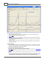
From top to bottom, here's what you see:
1. Title bar. Shows the name of the selected results data file. You can have multiple results files
loaded and multiple Graph windows open at a time.
2. Menu bar 12
3. Toolbar with one-click access to the program's major functions. Hover the pointer over a button to
see a brief description of that command.
4. The large graph charts the data as a LOD (or LR) score profile. The higher the LOD, the greater the
evidence for a QTL.
5. The smaller graph at the bottom is the QTL effects window, showing additive or dominant effects or
R2 or TR2 or S values.
Graph window tips
You can add several result files so they display at the same time on the current graph. You might
want to run your data through the IM, CIM, and MIM analysis methods, for example, and then pull
them all into the same graph to see how they compare.
Peaks above the threshold line indicate a QTL.
A high LOD value on the graph indicates a good QTL candidate.
Right-click on the graph to see appropriate commands. (Commands described in the Graph windowMenus 12 topic.)
You can minimize the Graph window to the bottom of the Main window; a small bit of the title bar is
visible.
You can have the same result file open in several windows at the same time. This might be useful if
you're testing various viewing parameters. To do this, minimize the current Graph window, go back
to the Main window, ensure the result file is still active, and click the Graph toolbar button.
© 2010 N.C. State University, Bioinformatics Research Center
WinQTLCart Windows & Menus
Related topics
Graph Window - Menus 12
Tracing coordinates on the graph 19
Selecting traits for graph display 20
Selecting chromosomes for graph display
Setting display parameters 21
Setting a test hypothesis 23
Showing QTL information 24
19
21
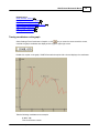
Tracing coordinates on the graph
Select Settings>Trace Coordinate in Graphic or click
. As you move the cursor around the screen,
note that the graph coordinates are displayed in the graph's upper right corner.
Double-click a point on the graph; WinQTLCart marks that point with a dot and displays the coordinates.
Take the following coordinates as an example:
(1, 46.7, 3.0)
1=the chromosome number
© 2010 N.C. State University, Bioinformatics Research Center
20
Windows QTL Cartographer 2.5
46.7=the cM location along the chromosome
3.0=the LOD score
After marking one or more points, copy the graphic to the clipboard (File>Copy to Clipboard) for use in
another application or for publication.
Re-select the command to toggle the coordinate display; WinQTLCart also clears from the display the
coordinate points you selected.
Related topics
Setting display parameters
21
Selecting traits for graph display
Select Traits>Select Trait(s)… or click
when you want to focus the graph on only a few traits,
rather than all of the traits in the data. Selecting the command displays the Select Traits dialog.
Click anywhere in a column to toggle display of the trait in the Graph window.
In the screen shot above, the Trait 1 Deletion cell is cleared, meaning this trait will be displayed. An
asterisk in the Deletion cell a trait means it will not be displayed.
Click Select All to show all the traits.
Click Select First to show only the first trait.
Click Help to display help text for this dialog.
Note
You cannot change the display order of traits. However, you can change the display order of
chromosomes.
© 2010 N.C. State University, Bioinformatics Research Center
WinQTLCart Windows & Menus
21
Selecting chromosomes for graph display
Select Chrom>Select Chroms… or click
when you want to focus the graph on only a few
chromosomes, rather than all of the chromosomes in the data. Selecting the command displays the
Select Chromosomes dialog. Use this dialog both to select chromosomes for display and to juggle their
display order.
The lower text field shows the chromosomes and the order in which they will be displayed.
To delete a chromosome from the graph display, click the cell in the Delete row below that
chromosome. An asterisk in a field means the chromosome will not be displayed; a clear field
means the chromosome will be displayed. Click the Deletion cell to toggle display on and off.
In the screen shot above, the Deletion cells for 1, 2, 3, and 6 are cleared, meaning those
chromosomes will be displayed. When a chromosome is removed from the display, its number
disappears from the lower text field, also. In the box above, clicking the empty cell under "3" would
remove chromosome chromo3 from the graph display.
To reorder chromosomes, click on a number in the Chromosomes row. It swaps places with the
next displayed cell to its right. Clicking the last displayed cell swaps it with the first displayed cell.
Example: In the screen shot above, clicking 1 will swap 1 and 2, and the display order will be 2 1 3
6. Clicking 3 will swap 3 and 6, so the display order would be 1 2 6 3. Clicking 6 will swap 6 and 1,
so the display order would be 6 2 3 1.
Click Select All to show all the chromosomes.
Click Select First to show only the first chromosome.
Click Help to display help text for this dialog.
Setting display parameters
Select Settings>Display Parameters or click
from the toolbar to display the Set Graph Display
Parameters dialog. Use this dialog to refine the display, change font sizes and colors used, and so on.
© 2010 N.C. State University, Bioinformatics Research Center
22
Windows QTL Cartographer 2.5
Show LOD profile as block graph view. Check to show color block for LOD / LR profile instead of line
curve. Use continuously or block radio button to set the total colors in color block display.
Ratio between effect window size and LOD window size. Use the spin dials to affect the display
ratio. You can choose, for example, to make the LOD window the same size as the effect window by
selecting 1:1. By default, the LOD window is 3 times the effects window size.
Title. Enter a title for the graph display. Use the X and Y coordinate boxes and the Font size box to
precisely place the title so it looks as you want.
Show QTL info. Check to toggle display of QTL information. See Showing QTL information
information.
24
for more
No LOD window. Check to suppress display of the LOD / LR graph window (upper window) and only
show the effect window.
No LOD line. Check to suppress display of the LOD / LR line curve in upper window.
© 2010 N.C. State University, Bioinformatics Research Center
WinQTLCart Windows & Menus
23
Legend on right. Check to show the legends to the right of the graphs. Uncheck to show the legends
above the graphs.
Show trace hairs. By default, WinQTLCart will not show X and Y cross hairs when you select use the
Trace Position command. Check this box if you do want to see the cross hairs.
Number of scale lines for X axis. Specify the number of hash marks spread across the cM scale of
the graph.
Number of scale lines for Y (LOD) axis. Specify the number of hash marks spread along the LOD
scale.
Number of scale lines for Y (effect) axis. Specify the number of hash marks spread along the effect
scale of the graph.
Space between two chromosomes. Specify a distance as a percentage of the graph scale to
separate the chromosomes in the graph. (Put in about 5 or 10 to see the effect.)
Threshold value for traits. Select a trait from the drop down list and enter a number to set as that
trait's threshold value. Click the Set all traits with this value button to impose a consistent threshold on
all displayed traits.
Trait color and line styles. Select a trait from the drop down list. Press the Color button to select its
color; select a Line Style from the drop down list to further differentiate it from other traits in the display.
Maximum LR value in graph. Check and input a value to limit the max LR (not LOD) value into the
value for the LOD / LR curve line, default value is max LR value in the selected chromosomes and traits.
Minimum LR value in graph. Check and input a value to set the minimum LR (not LOD) value into the
value at Y-axis, default value is 8.0.
Marker label font size. To adjust marker label's font size after selecting showing marker label in LOD /
LR window.
Setting a test hypothesis
Select Setting>Test Hypothesis to play with the results further by trying out different LOD / LR and
effects (additive, dominant, R2, TR2, S) settings on the displayed results.
Note: This option is only for crosses with three kinds of genotype such as SF2.
© 2010 N.C. State University, Bioinformatics Research Center
24
Windows QTL Cartographer 2.5
This dialog is fairly self-explanatory. The Hypothesis definitions box describes the conditions for each
hypothesis, with a=additive and d=dominant. The LR setting box describes pre-set likelihood ratio
hypotheses.
Click OK to apply the selected hypotheses options to your display.
Showing QTL information
Select Effects>Show QTL Information… or click
on the toolbar to display the Show QTL Information
dialog. From here, you can show QTLs from a simulation parameter file or show summary QTL
information from the likelihood ratio graph peaks.
Select the Open QTL information file option and then the Browse… button to select a file that has the
QTL positions and effects settings you want to use for the display.
Select the Show one or two LOD interval options, as desired, to show empiric QTL confidence
intervals—95 percent is one LOD and 99 percent is two LOD.
Select the Automatically locate QTLs option to specify parameters WinQTLCart will use to find QTLs
in the results. Use the spin dials to specify the minimum acceptable cM range that defines a QTL peak;
if the peak's distance is less than this value, then the highest peak will be considered a QTL. The
minimum acceptable LOD scale as measured by the highest and lowest points of a QTL peak on the
graph. Both of these requirements must be met for a peak to be considered a QTL.
© 2010 N.C. State University, Bioinformatics Research Center
WinQTLCart Windows & Menus
Related topics
Creating simulation data
25
51
WinQTLCart Procedures
Setting the working directory
By default, WinQTLCart looks for data files and other working files in its home directory (typically C:
\NCSU\WinQTLCart) or directory of last opened source data (mcd) file. WinQTLCart saves all files it
creates to the current working directory.
But if your data files reside in another directory or on a network drive, you can tell WinQTLCart to look for
and save its files there.
1.
Select Tools>Set Working Directory to display the Set Working Directory dialog.
2.
To change the directory, click Modify…, navigate to the directory you want, and click OK. The
new directory appears in the Set Working Directory dialog.
3.
Click Set.
Importing and exporting
Importing files
Unless the files you're working on have already been saved as WinQTLCart mapping source data files
(files with a .MCD extension) or are already in the .MCD format 39 , then you need to import them into
WinQTLCart. WinQTLCart will read in the files, verify the data formatting, and save the files in .MCD
format automatically.
WinQTLCart can import files from the following applications:
Application
Formats supported
MapMaker/QTL
.MAP – Map file
.MPS – Map file
.RAW – Cross data file
QTL Cartographer
.INP – Map and Cross data files
© 2010 N.C. State University, Bioinformatics Research Center
26
Windows QTL Cartographer 2.5
.MAP – Map file
.CRO – Cross data file
Microsoft Excel
.XLS
.CSV
Note If WinQTLCart displays an error message saying the file format is invalid or can't be recognized,
then the extension may be wrong or the file's formatting renders it unusable in WinQTLCart. Open
the file in Notepad and compare it to one of the sample files in the WinQTLCart directory.
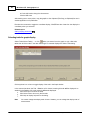
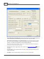
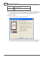
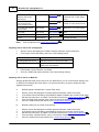
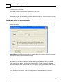
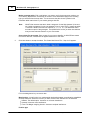
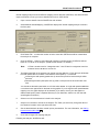
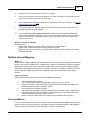
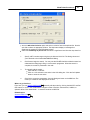
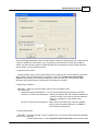
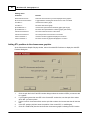
Importing source data files
1.
Select File>Import. The Source Data Import dialog appears.
2.
Select the import option you want. The first extension listed for each option is for the Map file, the
second extension for the Cross Data file. After clicking Next, the second import dialog appears.
© 2010 N.C. State University, Bioinformatics Research Center
WinQTLCart Procedures
27
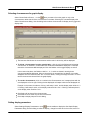
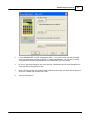
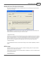
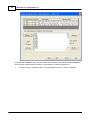
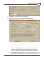
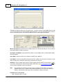
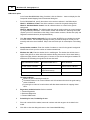
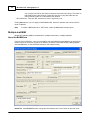
3.
For the MapMaker/QTL and QTL Cartographer options, you need to locate and select the Map
and Cross Data files by clicking the buttons. For Excel spreadsheets, you only need to specify
one spreadsheet (WinQTLCart disables the Cross Data button for Excel imports).
4.
By check "Infer map information from cross data file", WinQTLCart will infer map information from
cross data file by using Emap function.
5.
Enter a file name for the source data file that WinQTLCart will create. You don't need to specify an
extension—WinQTLCart will take care of that.
6.
Click the Finish button.
© 2010 N.C. State University, Bioinformatics Research Center
28
Windows QTL Cartographer 2.5
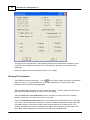
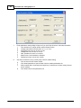
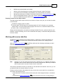
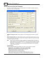
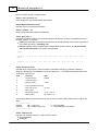
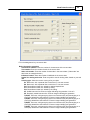
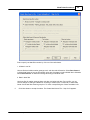
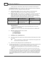
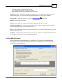
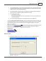
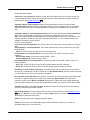
7.
Emap parameters setting dialog will pop-out if you use Emap function to infer map information.
Click the button to change random seed for Emap function.
Linkage map method can take value 10, 11, 12, or 13.
Segregation test size can be 0.01 to 0.20.
Linkage test size can be 0.15 to 0.49.
Now, permutaion function is not active.
Map function can be Haldane or Kosambi.
Objuective function can be SAL or SAR.
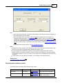
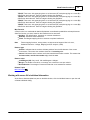
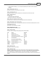
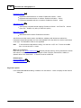
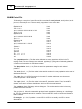
8.
Set anchor markers by using control group of Anchor marker setting .
Click to select anchor marker number.
Click button parameter to open window of Anchor marker parameters set
Select marker label, chromosome and position on chromosome for each marker (Current
anchor marker).
Click button OK to finish parameters set.
© 2010 N.C. State University, Bioinformatics Research Center
WinQTLCart Procedures
29
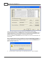
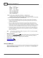
Note:
If the import was successful, you'll see a dialog saying the files were successfully imported and
the source data file has been saved.
If the import didn't work, the reason is likely that the files' formatting does not conform to a
standard WinQTLCart expects. To troubleshoot 86 this problem, open one of WinQTLCart's
sample files in Notepad and compare it to the file you specified. (The topic MCD file format 39
in this manual also describes the file format.) Correct any formatting problems in your specified
file and try importing again. If you're still unsuccessful, please contact WinQTLCart tech support
86 .
More detail help for Emap function, see QTL Cartograhper's manul.
Notes
WinQTLCart includes sample source data files for import. Run some tests using these files or open
them up to see the kind of data formatting WinQTLCart expects to see.
For Excel worksheets, WinQTLCart expects to see the following worksheet names in the file:
BasDat, ChrDat, and CroDat. WinQTLCart includes a sample file, NewMcd.xls, that demonstrates
the formatting it expects to see. (If you want, you can make a copy of NewMcd.xls and modify it for
your data.)
For INP format, one cross data file is needed if you use Emap to infer map information.
Related topics
Compatible programs and formats
1
Exporting source data and results
The following table summarizes WinQTLCart's export options:
Export …
…from the…
…to…
…in these formats…
Source data
Main window
QTL Cartographer
.INP – Map and cross data files
30
Source data
Main window
QTL Cartographer
30
© 2010 N.C. State University, Bioinformatics Research Center
.MAP – Map file
.CRO – Cross data file
30
Windows QTL Cartographer 2.5
Source data (minus
individuals with certain
OTrait values)
Main window
WinQTLCart
30
.MCD (with option to delete
individuals with a certain OTrait
value)
Source data (one or more
chromosome(s) with
reverse marker position)
Main window
WinQTLCart
30
.MCD (with reverse marker
position in some chromosomes)
Source data (with certain
selected traits)
Main window
WinQTLCart
30
.MCD (with some selected traits)
Source data
Main window
Microsoft Excel
31
.XLS
Results
Graph window
Microsoft Excel
31
.XLS
Results
Graph window
Text
Notes
.TXT (tab-delimited)
Files are exported to the current work ing directory
25
.
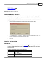
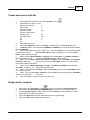
Exporting source data to QTL Cartographer
1.
2.
With the source data displayed in the Main window's Data pane, select File>Export.
In the Export Source Data dialog, select one of the following options:
Select this…
…to output these files
QTL Cartographer INP format
.INP files for both the map and cross data
QTL Cartographer OUT format
.MAP for the map file
.CRO for the dross data file
3.
4.
Edit the Map or Cross filenames, as needed.
Click OK. WinQTLCart exports the files to the current working directory.
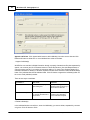
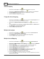
Exporting source data to an MCD file
Although WinQTLCart saves source data to its own .MCD format, you can use the export dialog to strip
an .MCD file of individuals with OTrait values. You would do this when you want to analyze the data
separate from the traits.
A.
MCD file (delete individuals with a certain OTrait value)
1.
2.
3.
4.
5.
With the source data displayed in the Main window's Data pane, select File>Export
In the Export Source Data dialog, select MCD file (delete individuals with a certain OTrait value).
Edit the source file name, as needed. The file will be saved to the current working directory 25 .
From the OTrait Value pull-down menu, select the trait to be stripped from the MCD file.
Click OK. WinQTLCart exports the file to the current working directory 25 .
B.
MCD file (reverse one or several chromosomes)
1.
2.
3.
4.
5.
With the source data displayed in the Main window's Data pane, select File>Export
In the Export Source Data dialog, select MCD file (reverse one or several chromosomes).
Edit the source file name, as needed. The file will be saved to the current working directory
From the Chrom. Number Edit Box, type in chromosome numbers separated by comma.
Click OK. WinQTLCart exports the file to the current working directory 25 .
25
.
© 2010 N.C. State University, Bioinformatics Research Center
WinQTLCart Procedures
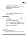
C.
31
MCD file (only selected traits are included)
1.
With the source data displayed in the Main window's Data pane, select File>Export
2.
In the Export Source Data dialog, select MCD file (only selected traits are included).
3.
Edit the source file name, as needed. The file will be saved to the current working directory
4.
From the Trait Number Edit Box, type in trait numbers separated by comma or hyphen.
5.
Click OK. WinQTLCart exports the file to the current working directory 25 .
Exporting results from the Graph window
25
.
The Graph window doesn't export results, per se (there's no Export menu), but you can save the results
in these formats:
WinQTLCart mapping result file (.QRT).
Excel file (.XLS), LR/LOD values to a worksheet labeled "LR", QTL information to a worksheet
labeled "QTLs", and points obtained through graph trace function to a worksheet labeled "Points".
Text file (.TXT), in a tab-delimited format.
Simply select the appropriate command from the Graph window's File menu, specify the directory and
filename in the Save As dialog, and click OK. WinQTLCart will display a confirmation dialog that the file
has been created.
Working with source data files
WinQTLCart's source data files have a .MCD extension. A .MCD file is a text file that adheres to a
specific format 39 that includes all the information WinQTLCart needs for QTL mapping analysis.
When you open a source data file 32 , WinQTLCart verifies the file's formatting and displays its basic
information in the Main window's Form pane.
Note
Although you can open other text and result files in WinQTLCart, only .MCD file information is
displayed in the Form pane. WinQTLCart will continue showing the last .MCD file you viewed in
the Form pane, even if you open or switch to text or result files.
The Summary Information box tells you the basics on the selected source data file. From here, you can
go ahead and select an analysis method, if you wish.
However, the form's buttons and pull-down lists let you look at the source data file in more detail and
also perform the following actions:
View information of markers, traits and other traits (also called categorical traits) in a formatted
way.
Add/edit/delete marker genotype data 32 for each chromosome in the file, including adding or
© 2010 N.C. State University, Bioinformatics Research Center
32
Windows QTL Cartographer 2.5
deleting individuals
Add/edit/delete trait values 33 and other traits
Edit map 34 and cross 35 information
Add new experimental data (individuals)
Try out different data configurations, such as retaining certain individuals' chromosomes
You may find that you need to add, edit, or delete data due to import errors. Some errors can be caused
by mistaking cross data for map data, and vice versa.
WinQTLCart's tools for editing marker, trait, and other information offer a safer and more organized
approach than if you were to do the same thing by hand in a text editor. If you need to alter the source
data's information in any way, it is highly recommended you use WinQTLCart.
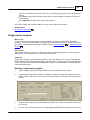
Opening source data files
There are several ways to open a prepared source data file from the Main window.
Select File>Open
Click the Open button on the toolbar
Use the keyboard command Ctrl+O
Double-click or right-click on the Source Files node in the Tree pane 10
Any of these methods opens the standard Windows Open dialog box. The dialog defaults to the current
working directory 25 . If you open an .MCD file from a different directory, WinQTLCart will save the
mapping result files to that location.
Also you can double click a .MCD file in Windows File Explorer to open the source data file
automatically.
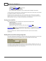
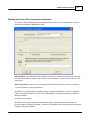
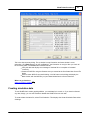
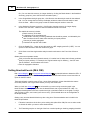
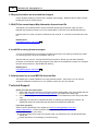
Working with a source file's marker genotype data
At the Source data view and modify pane on the Main window, select the chromosome you want to work
with from the pull-down list and click Markers button to open the Marker Information dialog.
At the Marker Information dialog, Marker Labels are the column headings, Individuals are the rows. You
can enlarge the dialog by dragging its border toward or away from the center of the screen. (The pointer
is a two-headed arrow when it is in the correct position.)
© 2010 N.C. State University, Bioinformatics Research Center
WinQTLCart Procedures
33
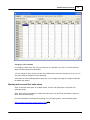
Changing a cell's contents
For modifying a cell's value, click in the cell and type in a new value. (Or, click in a cell and enter the
value in the Edit selected cell value field.)
You can change as many cells as you like. Click Update Cell to save your changes as you go. you can
click OK to save all changes and close the dialog.
Click Cancel to close the dialog without saving any of your changes (including any changes saved with
the Update Cell button).
Working with a source file's traits values
Traits: At the Trait values pane on the Main window, click the Trait View button to open the Trait
Information dialog.
Other Traits: If the source data file contains other traits, then click the OTrait View button to open the
Other Trait Information Dialog.
For more information on working with this dialog, and on modifying values, see the following topics:
Working with a source file's marker genotype data
© 2010 N.C. State University, Bioinformatics Research Center
32
34
Windows QTL Cartographer 2.5
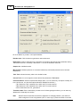
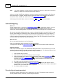
Working with a source file's basic information
At the Source data manipulations pane on the Main window, click the Basic Info button to open the
Manipulation of Basic Information dialog.
Symbol for missing trait value. Enter a symbol to use for missing traits value, based on your trait
data.
Marker translation table. Edit or add symbols you want to use for these genotype markers; you can
enter any alphanumeric character(s) as a symbol. These translations apply to the experimental design
you selected at the left of the dialog.
Note
WinQTLCart assumes that the A allele is diagnostic for the High (parental 1) line and the a
allele is diagnostic for the Low (parental 2) line. A minus sign (-) means the allele is unk nown.
WinQTLCart uses the numbers (2, 1, 0, 12, 10, -1) to determine how to encode the output of
the genotypes. The alphanumeric tok ens you enter here indicate how you have coded the
mark ers in the source data.
Cross Information
Select the experimental design option based on your data. You can select only one option.
B1. Backcross, with 1=parental line to which the F1 line was crossed.
B2. Backcross, with 2=parental line to which the F1 line was crossed.
Ri0. Recombinant inbred line, derived by doubled haploid lines.
Ri1. Recombinant inbred line, derived by selfing.
Ri2. Recombinant inbred line, derived by sib mating.
SF. Selfed intercross line. Enter an integer indicating the generation. Limit of 2.
RF. Randomly mated intercross line. Enter an integer indicating the generation.
© 2010 N.C. State University, Bioinformatics Research Center
WinQTLCart Procedures
T(B1)SF. Test cross, with genotyping done on an intercross (SF) and phenotyping on a cross
derived from that intercross. Enter an integer indicating the generation.
T(B1)RF. Test cross, with genotyping done on an intercross (RF) and phenotyping on a cross
derived from that intercross. Enter an integer indicating the generation.
T(B2)SF. Test cross, with genotyping done on an intercross (SF) and phenotyping on a cross
derived from that intercross. Enter an integer indicating the generation.
T(B2)RF. Test cross, with genotyping done on an intercross (RF) and phenotyping on a cross
derived from that intercross. Enter an integer indicating the generation.
35
(B1)
(B1)
(B2)
(B2)
Map Function
A map function is a mathematical relationship between recombination probabilities and map distances.
Select the function you want, based on the interference to be assumed.
Haldane. The default option. Assumes no crossover interference.
Kosambi. Assumes some interference.
Fixed. The Morgan mapping function. Assumes complete interference.
Note
These mapping functions, among others, are discussed at length in Ben Lui's book ,
Statistical Genomics: Linkage, Mapping and QTL Analysis (1998).
Distance type
Position. Indicates that the numbers indicate positions from the left telomere of the current
chromosome. This means the numbers should be in increasing order.
Interval. Indicates that the numbers are for the interval distance after a marker. This means that
the last number, and the last number only, should be zero.
Distance units
centiMorgan (cM). Very small. 100 centiMorgans=1 Morgan.
Morgan. The distance over which, on average, one crossover occurs per meiosis.
Recombination. Percentage of crossover events that occur between two markers.
Related Topics
MCD file format 39
Working with source file's individual information
At the Source data manipulations pane on the Main window, click the Individual button to open the Add
or Delete Individuals dialog.
© 2010 N.C. State University, Bioinformatics Research Center
36
Windows QTL Cartographer 2.5
Append and Delete. Click Append radio button to add individual(s) into active source data and click
Delete radio button to delete one or more individual from active source data.
1. Append individual(s)
WinQTLCart can read the individual information through a properly formatted text file (data separated by
spaces, not commas) and click Filename button to indicate the filename. (Use the Notepad button to
call up an empty text file if you need to do impromptu editing.) To check From Clipboard button if the
individual information is already in Windows clipboard. Please check the Data include individual label(s)
button if the individual data include individual label. Click OK button to append the individual(s) after set
the correct Total (individual) number.
There are two ways to read data.
If your data is...
Then click...
Comments
In a text file
Filename… to display the
Open dialog box.
In the Open dialog, select the
text file that has the values you
want to add and click OK.
On the Windows clipboard
Data from clipboard check You should select and copy
it to transfer the data to the the data in other text editor
edit window.
such as Windows notepad.
2. Delete individual(s)
In the Individual Number text edit box, enter the individual(s) you want to delete, separated by commas
or hyphen. Click OK button to finish.
© 2010 N.C. State University, Bioinformatics Research Center
WinQTLCart Procedures
37
Working with source file's chromosome information
At the Source data manipulations pane on the Main window, click the Chromosome button to open the
Chromosome and Markers Manipulation dialog.
Add and Delete. Click Add radio button to add a chromosome or a marker into active source data and
click Delete radio button to delete current chromosome or marker(s) in current chromosome from active
source data.
Select chromosome. Select one chromosome from the pull-down menu as the current chromosome.
1. Insert one marker in current chromosome
WinQTLCart can read the marker information through a properly formatted text file and click Filename
button to indicate the filename. To check From Clipboard button if the marker information is already in
Windows clipboard.
2. Insert one chromosome
WinQTLCart can read the chromosome information through a properly formatted text file and click
Filename button to indicate the filename. To check From Clipboard button if the chromosome information
is already in Windows clipboard.
© 2010 N.C. State University, Bioinformatics Research Center
38
Windows QTL Cartographer 2.5
3. Delete current chromosome
Click Delete current chromosome radio button and click OK button.
4. Delete marker(s) in current chromosome
Click Delete markers radio button and in the Marker Number text edit box, enter the marker(s) you want
to delete, separated by commas or hyphen.
Working with source file's trait information
At the Source data manipulations pane on the Main window, click the Trait button to open the Add or
Delete Traits dialog.
Add and Append. Click Append radio button to append trait(s) into active source data and click Delete
radio button to delete trait(s) from active source data.
1. Append trait(s)
WinQTLCart can read the trait information through a properly formatted text file and click Filename
button to indicate the filename. To check From Clipboard button if the trait information is already in
Windows clipboard. Please check the Data include trait label(s) button if the trait data include trait label.
Click OK button to append the trait(s) after set the correct Total (trait) number.
2. Delete trait(s)
In the Trait Number text edit box, enter the Trait(s) you want to delete, separated by commas or
hyphen.
© 2010 N.C. State University, Bioinformatics Research Center
WinQTLCart Procedures
39
Working with source file's other trait information
At the Source data manipulations pane on the Main window, click the OTrait button to open the Add or
Delete Other Traits dialog.
Add and Append. Click Append radio button to append other trait(s) into active source data and click
Delete radio button to delete other trait(s) from active source data.
1. Append other trait(s)
WinQTLCart can read the other trait information through a properly formatted text file and click Filename
button to indicate the filename. To check From Clipboard button if the other trait information is already in
Windows clipboard. Please check the Data include otrait label(s) button if the other trait data include
label. Click OK button to append the other trait(s) after set the correct Total (other trait) number.
2. Delete other trait(s)
In the OTrait Number text edit box, enter the Other Trait(s) you want to delete, separated by commas or
hyphen.
MCD file format
WinQTLCart .MCD source data files use tokens to indicate the meaning of data. This topic describes
valid tokens used in .MCD source data files.
The line numbers in this topic refer to the sample .MCD file, "NewMcd.mcd," which is included as part of
the WinQTLCart distribution.
Token #FileID (line 1)
© 2010 N.C. State University, Bioinformatics Research Center
40
Windows QTL Cartographer 2.5
File's ID number; usually a 10-digit number.
Token /* and */ (Lines 2 – 5)
Insert multiple-line comments between these tokens.
Token #bychromosome (Line 6)
Indicates start of chromosome information.
Token // (Lines 6 – 10)
Insert one-line comments after the double-slash.
Token –type (Line 7)
Indicates how marker positions are numbered along the chromosome. It takes one parameter that can
be either "position" or "interval".
Position indicates that the numbers are positions from the left telomere of the current chromosome.
So numbers should be in increasing order.
Interval indicates that the numbers are the interval distance after a marker. So the last number
and only the last number in the series should be zero.
-type
position
116.5
0.0
9.3
17.2
29.9
interval
9.3
7.9
12.7
8.8
38.7
14.1
52.8
5.0
57.8
14.6
72.4
4.2
76.6
16.6
93.2
3.8
97.0
18.5
1.0
115.5
0.0
Token –function (Line 8)
Indicates which map function is used to transfer recombination frequency (r) between markers to
distance in Morgan (M). The parameter can be an integer from 1 – 8. Haldane and Kosambi are the two
most useful map functions.
Code
Reference
Note
1
Haldane (1919)
Default
2
Kosambi (1944)
3
Morgan (1994)
4
Carter and Falconer (1951)
5
Rao et al. (1979)
0£p£1
6
Sturt (1976)
L
7
Felsenstein (1979)
-¥ < K < ¥, K ¹ 2
8
Karlin (1984)
Binomial, N > 0
"Fixed"
The following Haldane and Kosambi formula can be used to convert marker distance from r to M or vice
versa.
-----------------------------Haldane:
dM = -0.5ln(1-2r)
r = 0.5(1-exp(-2dM)
Kosambi:
dM = 0.25ln((1+2r)/(1-2r))
r = (1-exp(-4dM))/(2(1+exp(-4dM)))
-----------------------------Token –Units (Line 9)
Indicates unit of marker positions. There are three choices:
cM (centiMorgan)
M (Morgan)
© 2010 N.C. State University, Bioinformatics Research Center
WinQTLCart Procedures
41
r (Recombination frequency) - If you choose this parameter, then token -function should be 3
(Morgan)
Token –chromosome (Line 10)
Indicates total number of chromosomes for source data.
Token –maximum (Line 11)
Indicates the maximum number of markers for a chromosome for all of the source data.
Token –named (Line 12)
Either yes or no.
Yes means markers have names
No means markers will not have names.
Token –start and –end (Line 13 and Line 55)
Use these tokens to start and end the marker position data of all chromosomes.
Token –Chromosome (Line 14, 28, and 41)
Indicates chromosome name. The marker position data for this chromosome will start with the next line.
Token #bycross (Line 56)
Indicates that cross information is to begin.
Token –SampleSize (Line 57)
Indicates sample size or individual number.
Token –Cross (Line 58)
Indicates codes for crosstype mating design (see the following table).
Code
Design
Examples
Bi
Backcross to Pi
B1, B2
Bij
Backcross j times to Pi
B13, B25
SFi
Selfed generation i intercross
SF2, SF6
RFi
Randomly mated generation i intercross RF2, RF3
RI0
Doubled haploid
RI0
RI1
Recombinant inbred via selfing
RI1
RI2
Recombinant inbred via sib mating
RI2
T(Bi)SFj
Testcross of SFi to Pj
T(B1)SF3
T(SFi+j)SFi
Testcross of SFi for j generations
T(SF4)SF3
T(Bj)RFi
Testcross of RFi to Pj
T(B1)RF3
T(D3)SFi
Design III
T(D3)SF5
Token –traits (Line 59)
Indicates trait number of source data.
Token –otraits (Line 60)
Indicates other trait number of source data. Other trait (also called a categorical trait) is the trait with
qualitative or categorical values, such as sex; color, and so on. Other traits can be used as factors that
can be "regressed out" in regression analysis. This means a regression of the quantitative trait of
interest on the categorical trait will have been performed and the residuals used as the phenotypes in the
analysis.
© 2010 N.C. State University, Bioinformatics Research Center
42
Windows QTL Cartographer 2.5
Token –missingtrait (Line 61)
Indicates the symbol for missing trait value.
Token –case (Line 62)
Either yes or no.
Yes means all comparisons are case dependent.
No means all names of individuals, markers and traits are converted to lower case to make
comparisons.
Token –TranslationTable (Line 62)
The token with the table (next 6 lines of data) will define how marker genotype data are translated. There
are six rows and three columns (18 positions) in the table. Here is the default translation table:
-TranslationTable
AA
2
2
Aa
1
1
aa
0
0
A- 12 12
a- 10 10
-- -1 -1
The first column is the genotype. The program assumes that the A allele is diagnostic for the High
(parental 1) line and the a allele is diagnostic for the Low (parental 2) line. A minus sign (-) means
the allele is unknown (missing). Dominant as well as co-dominant markers can be encoded.
The middle column is how the output of these genotypes will be encoded.
The third column is how you will code the marker genotype data in this source data file. Just about
any set of tokens can be used for the third column (corresponding to your dataset), but DO NOT
change the first two columns.
The above TranslationTable maps 2 to 2, 1 to 1, 0 to 0, etc. Just about any set of tokens
can be used for the third column, but DO NOT change the first two columns. If you encoded
your P1 homozygotes as BB, heterozygotes as Bb, etc, your translation table might appear as:
-TranslationTable
AA
2 BB
Aa
1 Bb
aa
0 bb
A- 12 B
a- 10 b-- -1 --
Anything in the data file that is not recognized (doesn't match something in
column 3) will become unknown (-1) in the output.
Important: You need all 18 tokens following the -TranslationTable token and the
first two columns can't be altered. You should only alter the last column.
Token –start markers and –stop markers (Line 70 and Line 109)
Use these tokens to start and end the marker genotype data of all chromosomes. Please keep the
same chromosome and marker order as the data between token –start and token -end above.
You can organize the data by marker or individual:
Order by marker: For each marker, you provide the genotype data for all individuals. The order of the
© 2010 N.C. State University, Bioinformatics Research Center
WinQTLCart Procedures
43
individuals must be the same for each marker.
Order by individuals: For each individual, you provide the genotype data for all markers (all
chromosomes). The order of chromosomes and markers has to be the same.
-start individuals markers
Ind1 2 2 1 1 2 2 2
Ind2 2 2 2 1 2 1 2
Ind3 2 2 2 2 2 1 2
Ind4 2 1 2 2 2 2 1
Ind5 2 1 2 2 2 2 1
-stop individuals markers
2
2
1
1
1
2
1
1
1
1
Note that the tokens are different and the first column is the individual's label.
Token –start traits and –stop traits (Line 110 and Line 114)
Use these tokens to start and end the trait values. The data should be organized by the trait's order for
the trait value. That is, for each trait, you give the trait value of all individuals. If organized by the
individual, then for each individual, you provide the trait value of all traits.
-start individuals traits 2 Trait_1 Trait_2 named
Ind1
5.0
15.0
Ind2
5.3
15.3
Ind3
6.2
16.2
Ind4
4.1
24.1
Ind5
5.5
25.5
-stop individuals traits
Note that the tokens are different and there are trait number and trait labels after the token -start
individuals traits. The label "named" means data has trait names.
Token –start otraits and –stop otraits (Line 115 and Line 118)
Use these tokens to start and end the other trait values. The data must be organized by the other trait's
order; that is, for each other trait, you give the other trait value of all individuals. If you order by
individuals, then for each individual, you give the other trait value of all other traits.
Example:
-start individuals otraits 2 sex brood named
Ind1
M
1
Ind2
F
1
Ind3
M
0
Ind4
M
1
Ind5
M
1
-stop individuals otraits
Please notice that the tokens are different and there are other trait numbers and other trait labels after
the token -start individuals otraits. Label "named" means data has other trait names.
Token –quit and –end (Line 119 and Line 120)
Indicate the end of the source data file.
Token -population
Indicate the population number and the rest of .MCD filename.
Please notice that you should build one .MCD file for each population.
Example:
© 2010 N.C. State University, Bioinformatics Research Center
44
Windows QTL Cartographer 2.5
-population 4 env2-jun3.mcd env3-jun3.mcd env4-jun3.mcd
There are totally 4 populations and the 4 .MCD files include current file, and file "env2-jun3.mcd", file
"env3-jun3.mcd" and file "env4-jun3.mcd". All .MCD files should be in same directory.
Token -xchromosome
Indicate the X chromosome number and cross type that will not be the same as rest of chromosomes.
Creating a new source data file from raw data
WinQTLCart can help you convert your raw source data (including map and cross information) into
formatted MCD files. WinQTLCart can run analysis methods only on MCD files.
The goal of this process is to create a file that looks like the MCD data file (described in the MCD data
file format 39 topic). Although WinQTLCart can't automate this process for you, it does provide you with
tools to make a clean transition from raw source data to rigorously formatted data file.
The easiest way to work with this function is to have individual, properly formatted text files for each data
type (marker genotype, individuals, etc.). Individual files are quicker to select and import. Otherwise, you
do have to do a lot of copy and paste.
Here's a checklist of files you should have on hand, along with sample files in the WinQTLCart2.5\AddNew directory you can use to create your own files.
Chromosome labels and number. See 201-chlab-mknum.txt
Marker labels. See 301-mklab.txt that shows one file for all chromosomes.
Marker positions. See 302-mkpos.txt that shows one file for all chromosomes.
Marker genotypes. One file for all chromosomes and there are 4 different cases:
Case 1: Individual order with individual label, See 521-mkgen-ind-lab.txt
Case 2: Individual order without individual label, See 521-mkgen-ind-nolab.txt
Case 3: Marker order with marker label, See 541-mkgen-mk-lab.txt
Case 4: Marker order without marker label, See 541-mkgen-mk-nolab.txt
Trait values and labels. One file for all traits:
Case 1: Individual order with trait label, See 522-tt-ind-lab.txt
Case 2: Individual order without trait label, See 522-tt-ind-nolab.txt
Case 3: Trait order with trait label, See 542-tt-tt-lab.txt
Case 4: Trait order without trait label, See 542-tt-tt-nolab.txt
Other trait values and labels. One file for all other traits:
Case 1: Individual order with other trait label, See 523-ot-ind-lab.txt
Case 2: Individual order without other trait label, See 523-ot-ind-nolab.txt
Case 3: other trait order with other trait label, See 543-ot-ot-lab.txt
Case 4: other trait order without other trait label, See 543-ot-ot-nolab.txt
An alternative to use separate files is to create a single file holding marker genotype, trait, and other trait
information. But the data must be in individual order:
Case 1: has individual label, See 511-mkttot-lab.txt
Case 2: has not individual label See 511-mkttot-nolab.txt
1.
Select File>New to open the Create New Source File – Step 1 of 6 dialog box.
© 2010 N.C. State University, Bioinformatics Research Center
WinQTLCart Procedures
45
Fill in the dialog based on your source data.
Basic information group box
Chromosome number. Enter the number of chromosomes in the source data.
Trait number. Enter the number of traits in the source data.
Other trait number. Enter the number of other traits in the source data. ("Other traits" are
also known as categorical traits.)
Individual number. Enter the number of individuals in the source data.
Symbol for missing trait value. Enter a symbol to use for missing traits, based on your trait
data.
Crossing type. Select the correct cross type for your data:
B1. Backcross, with 1=parental line to which the F1 line was crossed.
B2. Backcross, with 2=parental line to which the F1 line was crossed.
Ri0. Recombinant inbred line, derived by doubled haploid lines.
Ri1. Recombinant inbred line, derived by selfing.
Ri2. Recombinant inbred line, derived by sib mating.
SF. Selfed intercross line. Enter an integer indicating the generation. Limit of 2.
RF. Randomly mated intercross line. Enter an integer indicating the generation.
T(B1)SF. Test cross, with genotyping done on an intercross (SF) and phenotyping on a
cross (B1) derived from that intercross. Enter an integer indicating the generation.
T(B1)RF. Test cross, with genotyping done on an intercross (RF) and phenotyping on a
cross (B1) derived from that intercross. Enter an integer indicating the generation.
T(B2)SF. Test cross, with genotyping done on an intercross (SF) and phenotyping on a
cross (B2) derived from that intercross. Enter an integer indicating the generation.
T(B2)RF. Test cross, with genotyping done on an intercross (RF) and phenotyping on a
cross (B2) derived from that intercross. Enter an integer indicating the generation.
© 2010 N.C. State University, Bioinformatics Research Center
46
Windows QTL Cartographer 2.5
Marker genotype table. Edit or add tokens you want to use for these genotype markers; you
can enter any alphanumeric character(s) as a token. These translations apply to the Crossing
type you selected from the drop down. You must ensure that the chosen symbols in this
translation table match those in your marker genotype data file.
Note
WinQTLCart assumes that the A allele is diagnostic for the High (parental 1) line and
the a allele is diagnostic for the Low (parental 2) line. A minus sign (-) means the allele
is unk nown. WinQTLCart uses the numbers (2, 1, 0, 12, 10, -1) to determine how to
encode the output of the genotypes. The alphanumeric tok ens you enter here indicate
how you have coded the mark ers in your source data.
Source data file stem name. Enter a name for your source data file. As WinQTLCart creates
new source data files, WinQTLCart will append extensions to this stem.
2.
Click Next button to accept the values. The Create New Source File – Step 2 of 6 appears.
Fill in the dialog based on your source data.
Map function. A map function is a mathematical relationship between recombination probabilities
and map distances. Select the function you want, based on the interference to be assumed.
Haldane. The default option. Assumes no crossover interference.
Kosambi. Assumes some interference.
Fixed. The Morgan mapping function. Assumes complete interference.
Position type
© 2010 N.C. State University, Bioinformatics Research Center
WinQTLCart Procedures
47
Position. Indicates that the numbers indicate positions from the left telomere of the current
chromosome. This means the numbers should be in increasing order.
Interval. Indicates that the numbers are for the interval distance after a marker. This means
that the last number, and the last number only, should be zero.
Position units
centiMorgans (cM). Very small. 100 centiMorgans=1 Morgan.
Morgan. The distance over which, on average, one crossover occurs per meiosis.
Recombination. Percentage of crossover events that occur between two markers.
Data-window. All the numbers you see here are place holders, waiting for you to input the real
data.
Edit window. Data from your raw data file (or in Windows clipboard) is copied to this window
first. You can edit data in this window.
Browse Displays Windows Open dialog so you can select the data file. Selecting the file copies
its contents to the Edit window.
Clipboard. Paste contents of Windows clipboard to Edit window.
Send Data. Check Include label if necessary, then click Send Data to update the data-window.
Notepad. Open a blank Notepad file, for use as a holding area for data, provide an editing
scratchpad, and so on.
3.
Click Next button to accept the values. The Create New Source File – Step 3 of 6 appears.
© 2010 N.C. State University, Bioinformatics Research Center
48
Windows QTL Cartographer 2.5
Click radio button Labels to input and send marker label information and click radio button Positions to
input and send marker positions information. Other operation is similar to above step 2.
4.
Click Next button to accept the values. The Create New Source File – Step 4 of 6 appears.
© 2010 N.C. State University, Bioinformatics Research Center
WinQTLCart Procedures
49
First to specify raw data file's number by click one of the radio button.
1. All data in one file
Use one file that includes marker genotype, trait, and other trait information. Select Data format 1
in Select data format of one raw file situation group box if the data include individual label. Otherwise
select Data format 2. All data must arrange according to individual order.
2. Data in three files
Use three files for marker genotype data, trait data, and other trait data. For each file, you can
choose arrange according to individual or according to marker (trait, or other trait) in Select data
format of three raw files situation group box. To check corresponding box if there are labels in file.
5.
Click Next button to accept the values. The Create New Source File – Step 5 of 6 appears.
© 2010 N.C. State University, Bioinformatics Research Center
50
Windows QTL Cartographer 2.5
Please notice that the buttons in this dialog is depend on the selections of previous dialog.
For marker genotype information, use Browse button to indicate the filename and Send Data button to
update the Data-Window. It is same for the trait value also. The Browse and Send Data button will be
disabled if there is no other trait, Otherwise, you can do the same as trait value.
Only one set of Browse and Send data button will be enabled if you choose one data file format in the
previous dialog.
Note: The Data file's format should be comparable with the setting of previous dialog. For example, if
there is no individual label in the genotype data file and you check the include individual labels button
in previous dialog. Then a warning message box will pop-out when you click the Send Data button in
Marker genotype filename group.
6.
Click Next button to accept the values. The Create New Source File – Step 6 of 6 appears.
© 2010 N.C. State University, Bioinformatics Research Center
WinQTLCart Procedures
51
This is the data summary dialog. The up window is map information and lower window is cross
information. Click Back button to do the modification if the information is not right. After you check all
the necessary data, click Finish button WinQTLCart will:
Verify the data and display error messages if the data file is incomplete or formatted
incorrectly.
Create the .MCD file using the filename stem you entered at the first Create New Source File
dialog.
Show a create .MCD file successful dialog, click OK button to the dialog and display the
Main window, with the MCD file you just created loaded into the Source Data form.
Where to go from here
Select an analysis method
2
Creating simulation data
To use WinQTLCart's results graphing abilities, you need data for it to work on. If you haven't collected
any data, though, you can still simulate a dataset that WinQTLCart can work with.
To create a data simulation file, select File>Simulation. This displays the Create Simulation Data series
of dialogs.
© 2010 N.C. State University, Bioinformatics Research Center
52
Windows QTL Cartographer 2.5
Fill in the blanks for yourself, or accept the defaults.
Random seed. Click the button to generate a new random seed.
Replications. Produce a file with many replications of simulation data with the same parameter setting.
The filename look like ***SimuRep-1.dat and the ***.mcd is the simulation .MCD file.
Sample size. Individual number.
Map function. Haldane (assumes no crossover interference) or Kosambi (assumes some crossover
interference).
Total Trait. Indicate how many traits in the simulation data.
Current Trait. You can change the current trait and set parameter of Trait mean.
Cross Information. Select an experimental design option. You can select only one option to modify at a
time. (At this time, only the three options below are available for selection.)
B1. Backcross, with 1=parental line to which the F1 line was crossed.
B2. Backcross, with 2=parental line to which the F1 line was crossed.
SF2. Selfed intercross line, generation 2.
Translation table. Edit or add tokens you want to use for these genotype markers; you can enter any
alphanumeric character(s) as a token.
Note
WinQTLCart assumes that the A allele is diagnostic for the High (parental 1) line and the a
allele is diagnostic for the Low (parental 2) line. A minus sign (-) means the allele is unk nown.
© 2010 N.C. State University, Bioinformatics Research Center
WinQTLCart Procedures
53
WinQTLCart uses the numbers (2, 1, 0, 12, 10, -1) to determine how to encode the output of
the genotypes. The alphanumeric tok ens you enter here indicate how you have coded the
mark ers in the source data. See the topic MCD file format 39 for more information.
Chromosome and marker information
Total chromosome number. The total number of chromosomes. Click the spin dial to the
right of this field to select more or fewer.
Current chromosome. Shows the active chromosome you're working on. Click the spin dial to
the right of this field to select a new chromosome. You'll see the new chromosome's
information in the Distance and Label boxes to the right.
Markers for chromosome. Total number of markers for this chromosome.
Average space between markers (cM). Produces marker positions randomly.
Variations of the marker positions (%). How many deviations are allowed, on average
Check Read marker positions from a text file and click Browse to select a text file
containing that information. Also, select a marker distance type.
Position. Indicates that the numbers indicate positions from the left telomere of the current
chromosome. This means the numbers should be in increasing order.
Interval. Indicates that the numbers are for the interval distance after a marker. This means
that the last number, and the last number only, should be zero.
From QSI file. To produce the simulation data by loading a QSI file alone. In Step 3, you can save all
simulation parameters into a QSI file.
Filename. The file name of the MCD file that will be created.
Directory. The directory that the simulated MCD file will be created.
© 2010 N.C. State University, Bioinformatics Research Center
54
Windows QTL Cartographer 2.5
Next Trait. Click this button to reach each trait and you can set following parameters.
QTL numbers. Set the number of QTLs to appear in the file.
Heritability. Requires a value in the range 0.0 to 1.0. Default is 0.8.
Vd/Va. Dominant variance/Additive variance
Vi/Va. Epistatic variance/Additive variance
For the Additive, Dominant, and Epistatic effects you want to see in the simulation, you can select
the following:
Effects direction
Same—All values are positive
Both—Values are positive and negative
Sign's Ratio—Ratio of negative:positive.
Effects distribution
Equal—All effects have the same value
Normal—Values derive from normal distribution
Gamma—Values derive from gamma distribution
Parameter—Value for gamma distribution
Note
For more information on effects distribution and the additive, dominant, and epistatic effects,
please refer to the QTL Cartographer's manual.
After inputting the parameters in the previous two dialogs, the final dialog presents the data simulation
model you have built. Click in any cell to see that cell's values represented in the fields below.
Next Trait (or First Trait). Click this button to reach each trait.
Use the fields to edit a cell's contents. Click the Update button to write the change to the model.
Click Save to save your model to a .QSI (QTL Simulation Information) file. The current working
© 2010 N.C. State University, Bioinformatics Research Center
WinQTLCart Procedures
55
directory is selected as the default. (Click the X in the dialog's upper right corner to close without
saving.)
Click Load to load a .QSI file to this window. The file's values replace the values you see in the
current window.
Click Adjustment to adjust values for the entire genome.
Click OK to produce the simulation data file. You can then use that file for analysis.
Related topics
Showing QTL information
24
Single-marker analysis
When to use
For quick scanning of the entire genome (all chromosomes) to find best possible QTLs and identify
missing (or incorrectly formatted) data. Use single-marker analysis first to ensure your data file is clean;
then move on more sophisticated analysis methods, such as Interval Mapping 58 and Composite Interval
Mapping 60 .
How it works
Single-marker analysis is based on the idea that if there is an association between a marker genotype
and trait value, it is likely that a QTL is close to that marker locus.
Comments
Single-marker analysis can be somewhat useful for a quick look at data, but it has been superceded by
Interval Mapping and Composite Interval Mapping. IM and CIM are more thorough and accurate indicators
of QTL. The prime value of WinQTLCart's single-marker analysis is its identification of missing data that
could affect later analysis.
Running a single-marker analysis
1.
Open a mapping source data file (an .MCD file) into the WinQTLCart main window.
2.
Select Method>Single-Marker Analysis. WinQTLCart analyzes the data and displays the singlemarker analysis controls in the form pane. The information pane on the right includes the analysis
results.
3.
Select a trait for display from the Trait Selection pull-down list. All the traits present in the file will
be on the list.
4.
For each trait, the information pane on the right displays WinQTLCart's statistical summary of the
© 2010 N.C. State University, Bioinformatics Research Center
56
Windows QTL Cartographer 2.5
file. (You can view this summary in a larger window by clicking the Result button in the Statistical
Summary group box, just to the left of the information pane.)
5.
In the Single Marker Analysis group box, click Result to view the analysis result for the selected
trait. You can change the font used by the display window to make the results easier to read.
Click the Save… button in this group to save the marker analysis results to a text file.
6.
In the Statistical Summary group box, click Result to view the summary in a larger display
window. Click the Save… button to save the statistical results to a text file.
The statistical summary includes:
Basic summary of the data
A histogram for the quantitative trait
WinQTLCart's summary of missing individuals that should be present, as indicated by the
data. If markers show 0% data, there was likely an import problem.
Summary of marker segregation
Combines LR map QTL and Q stats
7.
Click the Graphic File… button to save the results to a QTL mapping result file (*.QRT). You can
open this .QRT file later to view the results as a graph.
8.
Click Close to end the single-marker analysis session and return to the Form View of Source
Data.
Qstats show some important results:
Tells you that the data were imported correctly. If a marker has 0% data, that indicates a problem
(likely an import problem). For example, the original marker may be *Marker_1, but QTL sees
that as *Marker-1, and the values won't match.
Tests for segregation distortion
Setting threshold levels (IM & CIM)
Both Interval Mapping 58 and Composite Interval Mapping 60 use threshold values to determine QTLs. If
you don't know the threshold value for a trait, you can have WinQTLCart find them out and use them as
inputs for the QTL search.
The threshold levels control the rate of Type 1 errors (false positives). A lower threshold value means
more false positives; but a higher value means you may miss more QTLs.
When you look at a result graph 17 , the horizontal line you see running across the graph is the
threshold level. When the graph peaks over the threshold level, that is good evidence for a QTL. So,
setting the threshold level in this form controls how high or low that line will sit on the graph. Too high
and you'll see no QTLs; too low and you'll see too many. (The threshold value can be changed later in
the Graph window.)
Getting a very accurate threshold level may take a long time. Recommendations are included in the
threshold procedures.
1.
Follow the instructions for the form you're working with (either IM or CIM). Be sure to select a trait
or all traits for which you want to set a threshold level.
2.
The Threshold group box on the right of the form controls inputting or obtaining mapping threshold
© 2010 N.C. State University, Bioinformatics Research Center
WinQTLCart Procedures
57
values for each trait. Select a different trait number to see the threshold value of that trait.
3.
Select whether you want to set the threshold levels manually or have WinQTLCart determine the
threshold via permutations.
If you...
Do this...
Comments
Know the threshold values you
want to use
Input them into the Manual Input
57 box
Don't know the threshold values
you want to use
Select By Permutations 57 to have Permutations take a long time to
WinQTLCart calculate them.
run. If 1 permutation runs for 10
seconds, than 1000 permutations
will take 2-3 hours.
Setting threshold levels manually
This analysis occurs before you start the QTL analysis.
Use this procedure to set the threshold for each trait manually. This is useful if you know the value for
each trait. Alternatively, select All Traits and apply this threshold setting to all the traits.
1.
From the Trait Selection pull-down, select a trait to find the threshold value for that trait. (The All
Traits selection is available for permutations only.)
2.
Click the By Manual Input option.
3.
Input a threshold value into the box.
4.
Optional: Click Set as Default if you want to assign the threshold value you entered to all traits.
Setting threshold levels via permutations
This analysis occurs before you start the QTL analysis.
Setting values via permutations allows WinQTLCart to empirically estimate the genome-wide significance
threshold. Use this procedure if you don't know the value and you want WinQTLCart to find the optimal
threshold.
Threshold values will be filled in automatically for every trait according to significance level.
Following threshold analysis, WinQTLCart will display the results in the Data pane and save them in a
text file. The text file's name is displayed in the form after the analysis completes.
1.
2.
3.
From the Trait Selection pull-down, do one of the following:
Select one trait to find the threshold value for that trait.
Select All Traits to find threshold values for all traits.
Click the By Permutations option.
Enter a value for Permutation Times to set the permutation repeating times.
Note
4.
5.
If you want a quick run, use the default value of 300. But if you're going to publish, use
the 1000 value; this will tak e several hours to run but will yield very precise results. We
recommend starting this analysis before you leave for the day and letting it run
overnight.
Enter a value for Significance Level.
Click OK to begin threshold analysis.
© 2010 N.C. State University, Bioinformatics Research Center
58
Windows QTL Cartographer 2.5
Note
You cannot update the All Traits check box. WinQTLCart check s or clears this box based on
whether you select one or all traits from the drop down list.
After you click OK, WinQTLCart displays a countdown showing its progress through the file. When the
threshold analysis is complete, WinQTLCart will display the results in the Data pane and display the
results file's name. (WinQTLCart saves the file to the current working directory 25 .)
After setting the threshold value, move on to finish the IM
58
or CIM
60
analysis procedure.
Interval Mapping
What it is
Interval mapping (IM) is an extension of single-marker analysis 55 . In single-marker analysis, only one
marker is used in QTL mapping but effects are underestimated and the QTL position cannot be
determined. Interval mapping provides a systematic way to scan the whole genome for evidence of QTL.
IM uses two observable flanking markers to construct an interval within which to search for QTL. A map
function (either Haldane or Kosambi) is used to translate from recombination frequency to distance or
vice visa. Then, a LOD score is calculated at each increment (walking step) in the interval. Finally, the
LOD score profile is calculated for the whole genome. When a peak has exceeded the threshold value,
we declare that a QTL have been found at that location.
When to use it
IM is a good general standard to use for all datasets.
Use it in combination with or as part of a process including
You may wish to start with a single-marker analysis 55 and then run IM to further refine the analysis.
High-level process
Here's a quick overview of how to use WinQTLCart's IM implementation. The first few times you run this
analysis, go with the WinQTLCart default values for the form's parameters. The defaults provide the best
all-around parameter settings, especially for initial analysis sessions.
1.
2.
3.
4.
5.
6.
Select the IM analysis method.
Select the chromosome(s) and trait(s) you want to analyze.
Select a threshold level to apply to the selected trait(s). Select either By manual input 57 (the
WinQTLCart default) or By permutations 57 (to have WinQTLCart determine an optimum
threshold). See Setting the threshold level 56 for more information on the impact of each of
these choices.
Click OK to start the calculations for the threshold level.
Following threshold calculation, set IM form parameters 58 . Select a walk speed in cM. It's
recommended you use the same walk speed for your entire dataset. Don't reset the walk speed
between runs or your results will not be comparable.
Click Start to begin the analysis.
Running interval mapping analysis
WinQTLCart provides default values for the parameters in this form. The defaults provide the best allaround parameter settings, especially for initial analysis sessions.
© 2010 N.C. State University, Bioinformatics Research Center
WinQTLCart Procedures
59
Interval mapping analysis uses WinQTLCart mapping source data files (.MCD files). Use WinQTLCart's
import commands to move your source data files from text to .MCD format.
1.
Open a source data file into the WinQTLCart main window.
2.
Select Method>Interval Mapping. WinQTLCart displays the interval mapping analysis controls in
the form pane.
3.
Click Result File… to select the location of and to name the .QRT file that will be created when
the analysis is complete.
4.
Click the OTraits… button to enter other trait numbers or number ranges. WinQTLCart will use
these as a co-factor in the analysis. (WinQTLCart's default is no OTraits.)
Note
5.
OTraits is another term for "categorical traits." Use OTraits for back ground control as
nuisance factors we want to account for.
The Walk speed (cM) is the genome scan interval. and the default is 2. Click the spin dial beside
the Walk speed value to increase or decrease the walk speed by .5 increments.
Increasing the walk speed (greater than 2) means less precision but the analysis takes
less time.
Decreasing the walk speed (less than 2) yields a more precise result but will take more
time.
You should set the walk speed value once for the entire dataset. A single walk speed establishes
a consistent norm against which the data can be graphed. If you change the walk speed between
mapping runs, the graph displays will be skewed. (If you want to check your data against a
different walk speed, create a separate directory for your data files, and then run the new walk
speed against those files.)
6.
Select one or all chromosomes to include in the analysis.
7.
Select one or all traits to include in the analysis. The Traits you select may change the value of
the Threshold controls on the right side of the form.
8.
Set the threshold level via either manual input or permutations. For more information, see Setting
threshold levels (IM & CIM) 56 .
9.
Click Start to begin QTL mapping analysis.
Following the analysis, WinQTLCart will:
© 2010 N.C. State University, Bioinformatics Research Center
60
Windows QTL Cartographer 2.5
Create a QTL mapping result file (*.QRT) and open it in the Graph window
Create a QTL summary information file using the EQTL function.
Display a confirmation box asking if you want to display QTL summary information in the Main
window's Data pane.
Composite Interval Mapping
What it is
Composite interval mapping (CIM) adds background loci to simple interval mapping 58 (IM). CIM fits
parameters for a target QTL in one interval while simultaneously fitting partial regression coefficients for
"background markers" to account for variance caused by non-target QTL.
"In theory, CIM gives more power and precision than simple IM because the effects of other QTL are not
present as residual variance. Furthermore, CIM can remove the bias that would normally be caused by
QTL that are linked to the position being tested."
Background markers are usually 20-40cM apart.
High-level workflow
Here's a quick overview of how to use WinQTLCart's CIM implementation. The first few times you run this
analysis, go with the WinQTLCart default values for the form's parameters. The defaults provide the best
all-around parameter settings, especially for initial analysis sessions.
1.
2.
3.
4.
5.
6.
Select the CIM analysis method.
Select the chromosome(s) and trait(s) you want to analyze.
Select a threshold level to apply to the selected trait(s). Select either By manual input 57
(the WinQTLCart default) or By permutations 57 (to have WinQTLCart determine an optimum
threshold). See the Setting the threshold level 56 topic for more information on the impact of
each of these choices.
Click OK to start the calculations for the threshold level. This may take from several minutes
to several hours to run.
Following threshold calculation, set CIM form parameters 60 . Select a walk speed in cM. It's
recommended you use the same walk speed for your entire dataset. Don't reset the walk
speed between runs or your results will not be comparable.
Click Start to begin the analysis. The analysis may take from 20 minutes to several hours to
run.
Running composite interval mapping analysis
WinQTLCart provides default values for the parameters in this form. The defaults provide the best allaround parameter settings, especially for initial analysis sessions.
Composite interval mapping analysis uses WinQTLCart source data mapping files (.MCD files). Use
WinQTLCart's import commands to move your source data files from text to .MCD format.
1.
Open a source data file into the WinQTLCart main window.
2.
Select Method>Composite Interval Mapping. WinQTLCart displays the CIM analysis controls in
the form pane.
© 2010 N.C. State University, Bioinformatics Research Center
WinQTLCart Procedures
3.
Click Result File… to select the .QRT file you want to create.
4.
Click the Control… button to display the Set CIM Control Parameters dialog.
61
4a.
For the CIM Model field, specify the markers to be used as cofactors in the CIM analysis:
Model 1: All Marker Control—Use all the markers to control for the genetic background.
Model 2: Unlinked Marker Control—Use all unlinked markers to control for the genetic
background.
Model 6: Standard Model—The default model that selects certain markers as control
markers by using additional parameters: control marker number and window size.
Selecting this model requires you to fill in extra fields on the dialog: Control marker
numbers, Window size (cM), and Regression method selection (all explained below).
4b.
Click Set control markers manually if you do not want WinQTLCart to automatically select
the control markers. This will display a dialog box after you start the analysis so that you can
© 2010 N.C. State University, Bioinformatics Research Center
62
Windows QTL Cartographer 2.5
manually select the control markers. Skip to step 10 for a description of this dialog box.
The Background Controls group box specifies the number of background controls and regression
type WinQTLCart should use in applying the selected CIM model.
4c.
Control marker numbers—Enter the number of markers to control for the genetic
background. WinQTLCart will use up to the number of markers entered here.
4d.
Window size (cM)—Enter the window size in centiMorgans. The window size will block out
a region of the genome on either side of the markers flanking the test site. Since these
flanking regions are tightly linked to the testing site, if we were to use them as background
markers we would then be eliminating the signal from the test site itself.
If the control marker number is… And if the window size is…
This is the result
The total number of markers
0.0
Model 6 reduces to Model 1
The total number of markers
Large (such as the size of the
largest chromosome)
Model 2
Zero
N/a
Model 3
Recommendations
Model 6 is good for starting an analysis. Start with the default values of 5 for control
markers and 10 for window size.
Increasing the number of control markers will allow better resolution for mapping linked
QTLs.
4e.
Regression method selection—Select a method.
1: Forward Regression
2: Backward Regression
3: Forward & Backward
4f.
Probability for into:, Probability for out:
4g.
If the OTrait number field is enabled, enter other trait numbers and their ranges to be included
in the model.
Note
4h.
5.
OTraits is another term for "categorical traits." Use QTraits for back ground control
as nuisance factors we want to account for.
Click OK to close the dialog and return to the CIM analysis form.
The Walk speed (cM) default is 2. The walk speed is the genome scan interval. Click the spin dial
beside the Walk speed value to increase or decrease the walk speed by .5 increments.
Increasing the walk speed (greater than 2) means less precision but the analysis takes
less time.
Decreasing the walk speed (less than 2) yields a more precise result but will take more
time.
You should set the walk speed value once for the entire dataset. A single walk speed establishes
a consistent norm against which the data can be graphed. If you change the walk speed between
runs, the graph displays will be skewed. (If you want to check your data against a different walk
speed, create a separate directory for your data files, and then run the new walk speed against
those files.)
© 2010 N.C. State University, Bioinformatics Research Center
WinQTLCart Procedures
63
6.
Select one or all chromosomes to include in the analysis.
7.
Select one or all traits to include in the analysis. The Traits you select may change the value of
the Threshold controls on the right side of the form.
8.
Set the threshold level via either manual input or permutations. For more information, see Setting
threshold levels (IM & CIM) 56 .
9.
Click Start to begin QTL mapping analysis. WinQTLCart will open a Save As dialog for you to
save the result file that will be created.
10.
If you selected Set control markers manually in step 4b, then WinQTLCart will display the
Select CIM Control Markers dialog box. Enter or edit the marker numbers you want to using the
text box; separate each number with a space. Click on the marker row's cells to toggle their
display in the text box.
When the analysis is complete
WinQTLCart will
Create a QTL mapping result file (*.QRT) and open it in the Graph window
Create a QTL summary information file using the EQTL function.
Display a confirmation box asking if you want to display QTL summary information in the Main
window's Data pane.
Multiple Interval Mapping
What it is
Multiple interval mapping (MIM) uses multiple marker intervals simultaneously to fit multiple putative QTL
directly in the model for mapping QTL. The MIM model is based on Cockerham's model for interpreting
genetic parameters and the method of maximum likelihood for estimating genetic parameters. MIM is
well suited to the identification and estimation of genetic architecture parameters, including the number,
genomic positions, effects and interactions of significant QTL and their contribution to the genetic
variance.
High-level process
Here's a quick overview of how to use WinQTLCart's MIM implementation:
1.
2.
3.
4.
5.
6.
Select the MIM analysis method.
Pick a trait you want to work with. (MIM works with only one trait at a time.)
Decide if you want to create a model using WinQTLCart's default search procedures or an
alternative (such as Forward, Backward, or CIM).
Run the analysis to generate the model.
Refine the model as needed by editing individual cells in the model, adding or deleting QTL,
searching and testing QTLs or epistatics, and re-estimating. This part of the analysis can
iterate for as long as you want to search for QTLs.
Save the model as a .MDS file (or as a result file using the Refine Model function).
About the MIM form
From the Source Data form, open a source data file and select Multiple Interval Mapping as the analysis
method. If there is more than one trait in the dataset, the Select Trait for MIM Analysis dialog appears.
Select a trait from the drop down list and Click MIM... button to open MIM form.
© 2010 N.C. State University, Bioinformatics Research Center
64
Windows QTL Cartographer 2.5
The MIM form appears. Before you can use this form, you need to load or create a MIM analysis model.
You can open existing files containing MIM model parameters or you can use WinQTLCart to create a
model. The following screen shot shows the MIM form with a model loaded and analyzed.
Model drop down list. Contains the list of MIM models to be used for the analysis. You can create or
load several different models for selection.
New Model / Add Model. Have WinQTLCart create a new inital MIM model or create additional MIM
model for analysis.
Save Model. Save the model you've created or modified to an .MDS file.
Load Model. Load an existing MIM model parameters file (.MDS). Click the button to display an Open
dialog; navigate to the .MDS file containing the parameters and click OK.
Summary. Click to create a text summary file and a graph result file (.QRT). At the prompts, confirm
you want to create the files. WinQTLCart by default saves them to the current working directory 25 , but
you can specify a different location and filename.
Note
The summary file information includes position, lik elihood ratio and effect of each QTL,
epistatic effects of QTL, partition of the variance explained by QTL (main and interaction
effects), and estimates of genotypic value of individuals based on the model.
Parameters for current model
QTLs. Number of QTLs in model
© 2010 N.C. State University, Bioinformatics Research Center
WinQTLCart Procedures
65
Epistasis. Number of epistatic genes in model
L(k). Likelihood of the mode, k is the QTL number.
BIC. Bayesian Information Criteria (BIC) value of the mode.
QTL Effects. Click to test additive, dominant and epistatic effects. The data pane under the form will
show the test results. You can select the text and then Edit>Copy to copy it to the clipboard.
Refine Model…. Select an option and click OK to refine the model
70
's parameters.
Add QTL. Adds a QTL to the model.
Del QTL. Select a QTL column and click Del QTL to delete that QTL from the model.
Cell Edit / Cell Update. Click on a cell in the model to select it and then update its value in this field.
Click the Cell Update button to write the value to the cell.
Close. Close the MIM form and return to the Source Data form. If you have not saved your work, you can
save your work at this time.
The Model. Occupies the right half of the form. Click the blue <<QTL cell to expand the model so it fills
the form pane; click the QTL>> cell to re-display the MIM form.
Creating MIM initial model
Click the New Model (or Add Model) button on the MIM form. The following Create New MIM Model
dialog appears. At the Create New MIM Model dialog, select an enabled option from the Initial MIM
model selection method group box.
© 2010 N.C. State University, Bioinformatics Research Center
66
Windows QTL Cartographer 2.5
Regression options
66
Regression forward selection on markers. Enables the Criterion… button
Regression backward selection on markers. Enables the Criterion… button
Forward and backward selection on markers. Enables the Criterion… button
CIM search option
68
Scan through composite interval mapping. Enables the Control… and From File… buttons.
(From File… displays only after you select this option.)
MIM search option
69
MIM forward search method. Enables the OK button
After finishing the initial model creation, the MIM form redisplays with the buttons enabled, the
Parameters group fields populated, the new model available in the drop down list, and the model values
on the right . The Parameters fields are now populated.
Note
To see the entire model without scrolling, click the blue <<QTL cell. To return to the MIM
form, click the blue QTL>> button.
Where to go from here
From here, you can refine the MIM model 70 , manually edit the model by clicking the Add QTL and Del
QTL buttons, or click in the model field to change the value of Position, Chromosome, Additive, or
epistatic values. Click Save Model… to save the model as a .MDS file.
Related topics
About the MIM form 63
Refining the MIM model
70
Regression options
In the Create New MIM Model dialog: If enabled, click the Criterion… button to display the Set Criterion
dialog box.
© 2010 N.C. State University, Bioinformatics Research Center
WinQTLCart Procedures
67
Select the BIC-related criteria option and select a criterion from the drop down list. Use the
spin dial to select an appropriate X Value. The Help button displays a message box
explaining the meanings of the BIC-related criteria.
Select the Probability of partial R^2 and select a significance level from the drop down list.
1.
Specify a QTL number range using the spin dials and click OK. The dialog closes and
you're returned to the Create New MIM Model dialog.
2.
Click Start to begin the search. You may see the WinQTLCart Main window's status bar
underneath the dialog begin filling in as the search progresses. When the search is
complete, the model is presented in the cells.
3.
To manually edit the model:
Click Add QTL or Del QTL
Click on a cell and enter a new value in the Cell editing box. Click the Cell Update
button to enter the new value.
4.
Click OK to accept the parameters, close the dialog and return to the MIM form. The
model you created is now displayed in the form.
Where to go from here
From here, you can refine the MIM model 70 , manually edit the model by clicking the Add QTL and Del
QTL buttons, or click in the model field to change the value of Position, Chromosome, Additive, or
epistatic values. Click Save Model… to save the model as a .MDS file.
Related topics
About the MIM form 63
Refining the MIM model
70
© 2010 N.C. State University, Bioinformatics Research Center
68
Windows QTL Cartographer 2.5
CIM search option
In the Create New MIM Model dialog: If enabled, click the Criterion… button to display the Set
Composite Interval Mapping Control Parameters dialog box.
1.
For the CIM Model field, specify the markers to be used as cofactors in the CIM analysis:
Model 1: All Marker Control. Use all the markers to control for the genetic background.
Model 2: Unlinked Marker Control. Use all unlinked markers to control for the genetic
background.
Model 6: Standard Model. The default model that selects certain markers as control markers
by using additional parameters: control marker number and window size. Selecting this model
requires you to fill in extra fields on the dialog: Control marker numbers, Window size (cM), and
Regression method selection (all explained below).
2.
Click Set control markers manually if you do not want WinQTLCart to calculate the number
of control markers. This will display a dialog box after you start the analysis so that you can
manually select the control markers. Skip to the end of this topic for a description of this dialog
box.
3.
Control marker numbers. Enter the number of markers to control for the genetic background.
WinQTLCart will use up to the number of markers entered here.
4.
Window size (cM). Enter the window size in centiMorgans. The window size will block out a
region of the genome on either side of the markers flanking the test site. Since these flanking
regions are tightly linked to the testing site, if we were to use them as background markers we
would then be eliminating the signal from the test site itself.
If the control marker number
is…
And if the window size is…
This is the result
The total number of markers
0.0
Model 6 reduces to Model 1
The total number of markers
Large (such as the size of the
largest chromosome)
Model 2
Zero
N/a
Model 3
Recommendations
Model 6 is good for starting an analysis.
The default values of 5 for control markers and 10 for window size should be good starting
points for Model 6.
Increasing the number of control markers will allow better resolution for mapping linked
QTLs.
5.
Regression method selection. Select a method:
1: Forward Regression
2: Backward Regression
3: Forward & Backward
6.
Probability for into:, Probability for out:.
7.
If the trait number field is enabled, enter trait numbers and their ranges to be included in the
model.
8.
Click OK to close the dialog and return to the Create New MIM dialog.
© 2010 N.C. State University, Bioinformatics Research Center
WinQTLCart Procedures
69
9.
Click the Criterion button. The Set Threshold dialog appears. Enter a threshold value or click
Default to accept the default value (recommended). Click OK to accept the value and close the
dialog and return to the Create New MIM dialog.
10.
Click the Start button to begin the search. The CIM form may display during the calculations.
When the search is complete, the model is presented in the cells.
11.
To manually edit the model:
Click Add QTL or Del QTL
Click on a cell and enter a new value in the Cell editing box. Click the Cell Update button
to enter the new value.
12.
Click OK to accept the parameters, close the dialog and return to the MIM form.
If you selected Set control markers manually in step 2, then WinQTLCart will display the Select CIM
Control Markers dialog box. Enter or edit the marker numbers you want to using the text box; separate
each number with a space. Click on the marker row's cells to toggle their display in the text box.
Where to go from here
From here, you can refine the MIM model 70 , manually edit the model by clicking the Add QTL and Del
QTL buttons, or click in the model field to change the value of Position, Chromosome, Additive, or
epistatic values. Click Save Model… to save the model as a .MDS file.
Related topics
About the MIM form 63
Refining the MIM model
70
MIM search option
1. At the Select Parameters dialog, select a model selection criteria from the drop down list:
BIC-M0 ---> c(n) = ln(n)
© 2010 N.C. State University, Bioinformatics Research Center
70
Windows QTL Cartographer 2.5
AIC
---> c(n) = 2
BIC-M1 ---> c(n) = 2ln(ln(n))
BIC-M2 ---> c(n) = 2ln(n)
BIC-M3 ---> c(n) = 3ln(n)
BIC-X ---> c(n) = 10*X*ln(n)
Score - 0.05 significant level
Score - 0.10 significant level
Score - 0.20 significant level
Score - X significant level
Note: The first 6 options are BIC search criteria. BIC = n*ln(Q*Q)+p*c(n)
n: sample size, Q*Q: residula varance of model, p: regressor (marker) number
Choose last 4 options (Score), WinQTLCart will use score statistics (not LR) to do the forward
search for both main and epistatic QTLs as initial MIM model.
2. Click the spin dial beside MIM walk speed in cM to select the walk speed. The smaller the
number, the more precise the model, but the longer the analysis will take. (We recommend
accepting the default value.)
3. Click OK. WinQTLCart builds the model based on the trait and the model parameters you
selected. Under the Cancel button in the form, WinQTLCart displays its progress as it works
through the file. The process may take several minutes or several hours, depending on your data.
You can safely minimize the WinQTLCart window and work on other apps in the foreground.
4. The MIM form redisplays with the buttons enabled, the Parameters group fields populated, the
new model available in the drop down list, and the model values on the right . The Parameters
fields are now populated.
Note
To see the entire model without scrolling, click the blue <<QTL cell. To return to the MIM
form, click the blue QTL>> button.
Where to go from here
From here, you can refine the MIM model 70 , manually edit the model by clicking the Add QTL and Del
QTL buttons, or click in the model field to change the value of Position, Chromosome, Additive, or
epistatic values. Click Save Model… to save the model as a .MDS file.
Related topics
About the MIM form 63
Refining the MIM model
70
Refining the MIM model
After you've specified the model and criteria for the search, the model and its values are loaded into the
MIM form. At this point, you can further refine the model. From the MIM form, click Refine Model to
display the Refine MIM Model dialog.
© 2010 N.C. State University, Bioinformatics Research Center
WinQTLCart Procedures
71
At the refine MIM model dialog, select a model selection criteria from the drop down list. Choose the first
6 options, WinQTLCart will do search, test, or optimizing in the principle of LR test and use BIC as
criteria. By select the last 4 options, WinQTLCart will use score statistics test and certain significant
level as search, test and optimizing criteria.
1. Optimizing QTL positions
Move main QTLs one by one along the chromosome to maximize LR or Score statistics (choose the
first 6 options is LR and otherwise is score statistics). Check box Test both main and epistatic
effects is only worked in score statistics testing. By check this check box, both main QTL and its
interaction with other QTL(s) are considered in score statistics calculation.
2. Searching for new QTLs
Main QTLs - Search for new main QTL(s) using LR or Score statistics test.
QTL interactions:
Interaction between Identified QTLs - Try to find more interaction among existing main QTLs.
1D Scan of 1 new QTL and Interactions - Search one new main QTL plus interaction between the
new QTL and QTL in the model by test the interaction
effect only. Aavailable in Score statistics test
situation.
2D Scan of 2 new QTL and Interaction - Search two new main QTLs plus interaction between
them by test the interaction effect only. Aavailable in
Score statistics test situation.
3. Testing existing QTLs
Main QTLs - Test each main QTL to see it is significant or not. The QTL will be deleted from the MIM
model if it's not significant.
In Score statistics test, to check Only QTLs without interaction check box will do test
© 2010 N.C. State University, Bioinformatics Research Center
72
Windows QTL Cartographer 2.5
only on those main QTL(s) that have no interaction with other main QTL(s). The reason is
that WinQTLCart is allow existing of main QTL that has no (very little) effect but has
strong interaction effect in score statistics test situation.
QTL Interactions - Test each QTL interaction to see it's significant or not.
Clicking Start returns you to a slightly modified MIM model, where the operation will continue until the
result is obtained.
Note
To create a MIM results file in .QRT format, select the MIM model summary option.
Multiple-trait MIM
Multiple QTL Mapping (MIM) for multiple-trait or multiple-environment in multiple-population .
About the Mt-MIM form
From the Source Data form, open a source data file and select Multiple Interval Mapping as the analysis
method. If there is more than one trait in the dataset, the Select Trait for MIM Analysis dialog appears.
Click Mt-MIM button to open MT-MIM Parameters and Analysis Dialog.
Result File. Click Result File button change the result filename and click + button to open the result
© 2010 N.C. State University, Bioinformatics Research Center
WinQTLCart Procedures
73
file with Windows notepad.
Control File. Click Control File button to change the control filename and click + button to open the
control file with Windows notepad. The control file includes all initial parameters setting in the dialog,
detail please to see Mt-MIM Control File 74 .
Population Group. Total population refers to the total population number in the source data.
Selected number indicates how many populations will be in the QTL mapping model. To use Index
edit box to indicate the index of selected populations comparing to all populations in original source
data.
Parameter setting for current population Group. Click the spin dial beside the Current population
value to set current population number first. Then to fill other parameters in the rest of group.
Note: The current population number depends on selected population number only. For example, if the
selected population number is 3, then the current population will be 1, 2, and 3 despite where these
population is located in source data file.
For each current population:
Total traits in current population. The number refers to the total traits (or environments) in the source
data.
Selected traits in current population. The number indicates that how many traits will be in the QTL
mapping model.
index. The number string indicates the index of selected traits.
Selected QTLs in current population. Click the spin dial to set the QTL number for current
population.
Chromosome String. Chromosome number for QTL1, QTL2, ...
Position (cM) String. Positions for QTL1, QTL2, ...
Selected Epistasis in current population. Click the spin dial to set the QTL interaction terms for
current population.
QTL-1. QTL number list. They are the first QTL number between two QTL interaction.
QTL-2. QTL number list. They are the second QTL number between two QTL interaction.
Pleiotropy vs. Close Linkage Test Group. The purpose of the test is to see that two or more QTL is
the same or not statistically. The QTL number list is in QTL Number String edit box. Please notice that
you can do the test for one or more population all together.
Genome wide test of QTL effects. The purpose of the test is to see that two group of QTL effects (QTL
main effect or epistatic effect) are the same or not statistically. Effect number is the QTL effect
numbers in a effect group. Effect1 and Effect2 indicate group 1 effects and group 2 effect respectively.
Each QTL effect includes three number that are population number, trait number and QTL effect number.
Trait Pair wise Test. Click Trait Pair wise Test button to open the control file and click + button to
open the control file with Windows notepad.
Refine Model Group. Click the pull-down menu to select a function (please to see Mt-MIM Functions
75 ) and click Go button to start calculation. Modifying Step Edit Box to indicate the walk step in cM
while searching through chromosomes.
Update. Click the button after changing parameters setting.
Finish. Click the button to finish Mt-MIM analysis and the software will remind you to save the
parameters setting into a new control file.
© 2010 N.C. State University, Bioinformatics Research Center
74
Windows QTL Cartographer 2.5
Mt-MIM Control File
The following is a example of control file used for source data file env1-jun3.mcd, env2-jun3.mcd, env3jun3.mcd, and env4-jun3.mcd. There are totally 4 populations in the source data.
-populations 3 1 3 4
#population-1#
-traits 3 1 2 3
-qtls 4 1 46.09 2 155.23 3 60.09 3 172.53
-epis 2 1 2 2 3
#population-2#
-traits 2 2 3
-qtls 3 1 46.09 2 155.23 3 60.09
-epis 1 1 3
#population-3#
-traits 2 1 3
-qtls 3 1 46.09 3 60.09 3 172.53
-epis 0
-pvsltest 2
-p 1 2 3 4
-p 3 2 2 3
-gqtltest 2
-str1 1 1 1 1 1 2
-str2 2 1 1 2 1 2
-end
line 1
line 2
line 3
line 4
line 5
line 6
line 7
line 8
line 9
line 10
line 11
line 12
line 13
line 14
line 15
line 16
line 17
line 18
line 19
line 20
Token -populations. (line 1) The first number indicates how many populations will be in the QTL
mapping model. The rest number(s) is/are selected population(s). (using index of selected populations
comparing to all populations in original source data.)
Token #population. (line 2, 6, 10) This is the star line of parameters setting for each selected
population.
Token -trait. (line 3, 7, 11) The first number is the total trait number for current population and the rest is/
are selected trait index.
Token -qtls. (line 4, 8, 12) The first number is the total QTL number and the rest are chromosome
number and position in cM for each QTL.
Token -epis. (line 5, 9, 13) The first number is the total QTL interaction number. Then, for each QTL
epistasis, there are two numbers that indicate which two QTLs that are interacted.
Token -pvsltest. (line 14) Pleiotropy vs. close linkage test. The number after the token is how many
populations that are in the test.
Token -p. (line 15, 16) One line started with -p token for each population of pleiotropy vs. close linkage
test. The first number indicates which population. Then the total QTL number to be test and followed by
the QTL indexes.
For example. -p 1 2 3 4, Population 1, to test QTL 3 and QTL 4 are actually one QTL or are two
different QTLs.
© 2010 N.C. State University, Bioinformatics Research Center
WinQTLCart Procedures
75
Token -gqtltest. (line 17) To test two sets of QTL effects (see token -str1 and -str2) have the same
effects or not. The number followed by the token is the QTL effect number of each set.
Token -str1 and -str2. (line 18, 19) Every three numbers (population, trait, and QTL) indicate a QTL
effect.
For example.
-gqtltest 2
-str1 1 1 1 1 1 2
-str2 2 1 1 2 1 2
This is to test the following assumption: population 1, trait 1, QTL effect 1 equal to population 2, trait 1,
QTL effect 1 as well as population 1, trait 1, QTL effect 2 equal to population 2, trait 1, QTL effect 2. or
not.
Token -end. (line 20) End of Mt-MIM Control File.
Mt-MIM Functions
In the Refine Model Group, you can select one of following functions from the pull-down menu.
1. Model parameter estimation
To do the parameters estimation for current model. The likelihood value is displayed in information
window on the bottom and the detailed result is in the result file. You can compare the likelihood values
between two QTL models (likelihood test) to do certain decision, such as the new QTL is significant or
not, The two QTL is the same or not etc.
2. Test all QTL effects
To test the value is zero or not for each of the QTL effects (additive, dominant, and epistasis).
3. Optimize QTL positions
To go through whole genome (you can set the walk speed, such 1.0 cM), find best position for each
QTL.
4. Search main QTL(s)
If you do not know the new QTL's chromosome and position, then to assign value -1 to the
chromosome string and WinQTLCart will search the best chromosome number and position for you
automatically.
5. Search epistasis interaction(s)
If you want to find the best QTL interaction, then assign value -1 to QTL-1 and QTL-2 and WinQTLCart
will find out the best QTL number 1 and QTL number 2 for you automatically.
6. Graphic and summary result
To obtain the graph result file and text summary file.
7. Test Pleiotropy in current population
© 2010 N.C. State University, Bioinformatics Research Center
76
Windows QTL Cartographer 2.5
To do the pleiotropy vs. close linkage test according to above parameter setting.
8. Genome wide test of QTL effects
To do the QTL effect(s) equality test according to above parameter setting.
9. Trait pairwise co-relation in current population
To calculate QTL co-relation between pairs of traits according to a control file (TPControl.txt).
Example of TPControl file:
#begin
1 gene_563 gene_2694 3 3 54.6 15 52.5 13 288.1
2 gene_563 gene_4898 2 3 54.6 15 52.5
3 gene_563 gene_5323 2 3 54.6 15 52.5
#end
The control file start with line of #begin and end with line of #end. For each line between is the
information for a pair of traits. The first number is the numbering, and second and third are the marker
labels for the first and second trait. After that is the total QTL number follow by chromosome number and
position for each QTL.
Bayesian Interval Mapping
WinQTLCart's Bayesian interval mapping (BIM) module is an implementation of the command-line BIM
library, provided courtesy of the R Project for Statistical Computing.
What it is
Bayesian interval mapping library R/bim provides Bayesian analysis of multiple quantitative trait loci
models. This includes posterior estimates of the number and location of QTL and of their effects.
Bayesian interval mapping for controlled experiment provides a nice complement to the classical
analysis for mapping QTLs. It is recommended that the standard IM, CIM, MIM, etc. analyses be run
first. The Bmapqtl implements Bayesian analysis for either a fixed or random number of QTLs.
(WinQTLCart's default is random.)
The program generates a random sample from the joint posterior of QTL and effects. Note that the BIM
estimates should generally agree with those of MIM, and should be similar to those from CIM.
BIM allows one to look deeper at the properties of those estimates, such as how effects estimates are
related to loci estimates. It also provides handy tools to explore research questions, such as the
posterior chance of multiple QTL in an interval.
How to use
The defaults are quite robust, and it is recommended you use them during your first BIM runs.
For more information on the BIM parameters
Please refer to the R implementation, particularly the function bmapqtl.options(). The best way to get
library(bim) is to already have R 1.9.0 installed on your PC.
1.
If you don't have R 1.9.0 installed on your computer, go to http://cran.r-project.org/
2.
Download the precompiled binary distribution of R (Linux or Windows is preferred.) Follow
© 2010 N.C. State University, Bioinformatics Research Center
WinQTLCart Procedures
3.
4.
5.
6.
Note
77
instructions for installation and run R.
While connected to the Internet, select R's Packages menu and select Install packages from
Bioconductor.
Scroll down to the "bim" package and click on it.
Use the R Help to get HTML Help.
Select Packages and click BIM from the list. There is an overview document but the options
are explained in detail in bmapqtl.options.
Pre-1.9.0 releases of R can get the bmapqtl pack age from the CRAN website cited above.
Bioconductor is a companion project to CRAN focused on biological applications. Brian
A quick summary of BIM implementation in a previous version of QTL Cartographer can be found at
http://www.cs.wisc.edu/~yandell/qtl/software/Bmapqtl/Bmapqtl.pdf.
High-level workflow
The first few times you run this analysis, go with the WinQTLCart default values for the form's
parameters. The defaults provide the best all-around parameter settings, especially for initial analysis
sessions.
1.
2.
3.
4.
5.
Select the BIM analysis method.
Select the chromosome(s) and trait(s) you want to analyze.
Click New Seed to select a new random seed.
Click Parameters… and set the BIM parameters of interest to you.
Click Start to begin the analysis.
Running Bayesian interval mapping analysis
1.
2.
Open a source data file into the WinQTLCart main window.
Select Method>Bayesian Interval Mapping. WinQTLCart displays the BIM analysis controls in the
form pane.
3.
4.
5.
Click Result File… to name the .QRT file you want to create and to specify its location.
Click New Seed to generate a new random seed number.
Select one or all chromosomes from the Chromosome Selection drop down to include in the
analysis.
Select one or all traits from the Trait Selection drop down to include in the analysis.
Click the Parameters… button to display the Set BIM Parameters dialog.
For more information on each of these parameters, please refer to the R bmapqtl documentation
cited in the topic, "Bayesian Interval Mapping 76 ".
Click Start to begin QTL mapping analysis.
6.
7.
8.
© 2010 N.C. State University, Bioinformatics Research Center
78
Windows QTL Cartographer 2.5
Multiple-trait analysis
Most of the analysis methods in WinQTLCart work on traits one by one. The multiple trait analysis lets
you pick and choose the traits you want to work with jointly. This allows you to perhaps derive and
correlate structures from among many separate traits.
1.
2.
3.
4.
5.
6.
Open a source data file in WinQTLCart. If the data contains multiple traits, WinQTLCart enables
the Method menu's Multiple Traits Analysis command.
Select Method>Multiple Traits Analysis. The Multiple Traits Analysis dialog appears.
WinQTLCart disables portions of the dialog box that cannot support analysis of the selected data
file.
B1 crosstype has additive effects and enables only method selection
F2 crosstype has dominant effects and enables hypothesis test selection (open the
WinQTLCart sample file "cod.mcd" for an example)
Select the analysis method you want to use, IM or CIM.
Select the traits you want to use in the analysis. Click the Trait List button to see available traits
for selection. In the Trait selection text box, enter the traits you want to use, separated by
commas.
So, if you want to use traits 1, 4, and 5, you would enter "1, 4, 5" (without the quote marks).
Click OK. The form pane takes on the standard IM/CIM look and function, but the countdown pane
prefixes the method with "Multiple Traits."
For permutation procedure, check Independent check box to randomize each trait independently.
Otherwise to keep the co-relationship among traits when doing randomization.
Refer to the IM
58
and CIM
60
procedures in this manual for more information on using the form.
Drawing a chromosome tree
You may need to use chromosome graphics when it's time to write an article on your research.
WinQTLCart displays all the source data file's chromosomes, including each chromosome's markers
and intervals, in a single display window that you can copy to the Windows clipboard.
From the Main window, with a source data file loaded, select Tools>DrawChrom to show the
Chromosome Graphic Display window.
© 2010 N.C. State University, Bioinformatics Research Center
WinQTLCart Procedures
79
This sample graphic shows you the chromosome names, the markers on the chromosomes, and their
distances.
Chromosome Graphic Display menus
File menu
Command
Function
Copy to Clipboard
Copies the graphs to the Windows clipboard.
Print Graphic
Print the graphic to a selected printer.
Exit
Closes the window. If you have unsaved data, you'll be prompted to save it.
View menu
Command
Function
Proportion of Marker Number
Show length of chromosome graph in proportion of marker number
Proportion of Chromosome Len Show length of chromosome graph in proportion of chromosome length
in cM
Next Page >>
If there are lots of chromosomes, displays the next group of graphs
First Page
If there are more than one screen of chromosomes, return to the first
page.
Add QTL positions…
Mark a QTL position on the chromosome. See Adding QTL positions to the
chromosome graphics 80 for more information.
© 2010 N.C. State University, Bioinformatics Research Center
80
Windows QTL Cartographer 2.5
Setting menu
Command
Function
Select Chromosomes…
Select the chromosomes you want displayed in the graphic.
Show Chromosome Name
Toggle between showing the chromosome name or its label
Font Size >>
Increase font size for graph
Font Size <<
Decrease font size for graph
Space Between >>
Increase the space between markers (graph gets longer)
Space Between <<
Decrease the space between markers (graph gets shorter)
Chromosome Name>>
Go to the next chromosome in the series
Chromosome Name<<
Go to the previous chromosome in the series
Column Number >>
Increase number of graphics displayed in a column
Column Number <<
Decrease number of graphics displayed in a column
Adding QTL positions to the chromosome graphics
At the Chromosome Graphic Display window, select View>Add QTL Positions to display the Add QTL
Positions dialog box.
1.
2.
3.
4.
5.
Click the spin dial in the Total QTL number dialog to select the number of QTLs you want to add
to a graphic.
If you're placing more than one QTL in the Current QTL number box, use the spin dial to select
which QTL you want to place.
For the In which chromosome field, use the spin dial to select the chromosome that will hold the
QTL.
In the QTL position (cM) field, enter the position of the current QTL, in centiMorgans.
Click OK. WinQTLCart places a band over the chromosome graphic indicating the QTL location.
© 2010 N.C. State University, Bioinformatics Research Center
WinQTLCart Procedures
A chromosome graphic before adding QTL positions...
...and after adding QTL positions
Tutorials
Import data files
Create source data file (*.mcd) by using different formats of data file(s).
Import data - INP format
1.
2.
3.
4.
5.
Start WinQTLCart and select menu item File>Import or click
.
Select QTL cartographer INP format and click Next button.
Click button Map File to select file "wqcart-map.inp".
Click button Cross Data to select file "wqcart-cro.inp".
Enter file name "wqcart_inp_In" in edit box and click button Finish.
Using Emap function
1.
2.
3.
4.
5.
Start WinQTLCart and select menu item File>Import or click
.
Select QTL cartographer INP format and click Next button.
Check "Infer map information from cross data file".
Click button Cross Data to select file "Csamp0.inp".
Enter file name "Csamp0_inp_In" in edit box and click button Finish.
Import data - OUT format
1.
2.
3.
4.
5.
Start WinQTLCart and select menu item File>Import or click
.
Select QTL cartographer OUT format and click Next button.
Click button Map File to select file "wqcart.map".
Click button Cross Data to select file "wqcart.cro".
Enter file name "wqcart_out_In" in edit box and click button Finish.
© 2010 N.C. State University, Bioinformatics Research Center
81
82
Windows QTL Cartographer 2.5
Import data - MapMaker format
1.
2.
3.
4.
5.
Start WinQTLCart and select menu item File>Import or click
.
Select Mapmaker/QTL format and click Next button.
Click button Map File to select file "mapmaker-samp.map".
Click button Cross Data to select file "mapmaker-samp".
Enter file name "mapmaker-samp_In" in edit box and click button Finish.
Import data - Excel format
1.
2.
3.
4.
Start WinQTLCart and select menu item File>Import or click
.
Select Microsoft Excel format and click Next button.
Click button Excel File to select file "wqcart-samp.xls".
Enter file name "wqcart-samp_xls_In" in edit box and click button Finish.
Import data - CSV format
1.
2.
3.
4.
Start WinQTLCart and select menu item File>Import or click
.
Select Microsoft CSV format and click Next button.
Click button CSV File to select file "NSimuB1-01-OnePop.csv".
Enter file name "NSimuB1-01-OnePop_in" in edit box and click button Finish.
Simulation source data file
1.
2.
Start WinQTLCart and select menu item File>Simulation or click
.
In step 1/3, set parameters as:
Sample size:
200
Trait mean:
15.85
Random seed:
any
Map function:
Haldane
Cross type:
B1
Translation table:
AA>2, Aa>1, A>*
Total chromosome number:
3
3.
Set The current chromosome as 1, Markers for chromosome 1 as 15, Average space
between marker as 9,
Variations of the marker position as 10%. Click button Set as
default for all chromosomes to set parameter for
other chromosome. Click button Next to step
2/3 dialog window.
4.
In step 2/3, set parameters as:
QTL numbers:
7
Heritability:
0.82
Additive effect:
Effects direction>Same
Effects distribution>Normal
Epistatic effect:
None by uncheck the check box
Filename:
"Nsimu-01"
Click button OK to step 3/3 dialog window.
5.
In step 3/3, Click button Adjustment to adjust all parameters. Click button Save to save the
parameter setting to file
"Nsimu-01.qpe". Click button OK to finish.
© 2010 N.C. State University, Bioinformatics Research Center
Tutorials
83
Create new source data file
1.
2.
Start WinQTLCart and select menu item File>New or click
.
Set parameters in step 1 of 2 as:
Chromosome number:
2
Trait number:
2
Other trait number:
1
Individual number:
125
Symbol of missing trait:
.
Crossing type:
B1
File stem name:
Test
AA
2
Aa
1
Aa
*
3.
Click OK to step 2 of 2.
4.
Click button Notepad to open file "Text.txt" in default directory (C:\NCSU\WinQTLCart).
5.
In Notepad, select chromosome label (CHROM-1, CHROM-2) and copy to Windows clipboard.
Minimize Notepad.
6.
Back to Create New Source File – Step 2 0f 2. Click button Paste to show chromosome labels
in Edit Window. Select
Chromosome Labels in Data Type Selection. Click button Send
Data to input chromosome labels.
7.
Select and copy Marker Number in Notepad. Click button Paste, click Marker numbers in
Data Type Selection and
click button Send Data to input marker numbers.
8.
Select and copy Marker Label and Position in Notepad. Click button Paste, Select Marker
positions in Data Type
Selection and click button Send Data. Answer "Y" in the dialog to
input marker labels and positions.
9.
Select and copy Marker Genotype and paste. Click Marker genotypes and click button
Send Data . Answer "Y" to
input marker genotype data.
10.
Select, copy and Paste Trait Value. Select Trait Values and click button Send Data. Answer
"Y" to input trait values.
11.
Select, copy and Paste Other Trait Value. Select OTrait Values and click button Send Data.
Answer "Y" to input other
trait values.
12.
Click button OK to create source data file (Test.mcd).
Single marker analysis
1.
2.
3.
4.
5.
Select Menu Item File>Open or click
to open source data file "wqcart-samp0.mcd".
Select Menu Item Method>Single Marker Analysis to open the Form of single analysis.
Use the poll-down menu to select a trait. Click button Result to show information of single
marker analysis or statistical summary.
Click button Graph File to produce result file and show in graph dialog.
Click button OK to finish single marker analysis.
© 2010 N.C. State University, Bioinformatics Research Center
84
Windows QTL Cartographer 2.5
Interval mapping
1.
Select Menu Item File>Open or click
to open source data file "mouse.mcd".
2.
3.
4.
5.
Select Menu Item Method>Interval Mapping or click
to open the Form of IM analysis.
Select By Permutation and click button OK to start threshold value calculation.
Click button Start to start IM analysis.
Click "Y" to show QTL summary in Text Window.
Composite interval mapping
1.
Select Menu Item File>Open or click
to open source data file "wqcart-samp0.mcd". You
can just click the tree item if the file has already been opened.
2.
Select Menu Item Method>Composite Interval Mapping or click
to open the Form of
CIM.
Click button Control to set the parameter. Set Control marker number as 8, Window size as
15.0, Other trait as 1,2 and click button OK to back.
Select All traits in trait selection pull-down menu.
Click button Start to begin CIM analysis.
3.
4.
5.
Multiple-trait analysis
1.
2.
3.
4.
Select Menu Item File>Open or click
to open source data file "wqcart-samp0.mcd".
Select Menu Item Method>Multiple Traits Analysis.
Select IM Method and input 1,3 in edit box for Multiple Traits Setting Dialog.
Click button Start to begin multiple traits analysis.
Multiple Interval Mapping
1.
Select Menu Item File>Open or click
to open source data file "wqcart-samp0.mcd".
2.
Select Menu Item Method>Multiple Interval Mapping or click
and select trait MECIAIA to
enter the Form of MIM.
3.
Click button New Model, click "Y", and click button OK to obtain an initial MIM model.
4.
Click button Refine Model. Select Optimizing position and click button OK.
5.
Click button Start to start QTL position optimization procedure.
6.
Click button Save Model to save the QTL model.
7.
Click button Refine Model. Select Searching for new QTLs and click button OK.
8.
Select Search for QTLs and click button Start for searching for more QTL.
9.
Click button Refine Model and optimize QTL position again.
10. Click button Test All to see LR values for each QTL in Text window.
11. Click button Save Model to save the QTL model again. You may change filename if you want to
keep the previous QTL model.
© 2010 N.C. State University, Bioinformatics Research Center
Tutorials
12.
13.
14.
15.
16.
17.
85
Click button Refine Model. Select Searching for new QTLs and click button OK. Select
Search for Epistasis and click button Start for searching for QTL interact (epistasis). Answer "Y"
to add the epistatic effect.
click button Refine Model. Select MIM Model Summary and click button OK.
Select Graphic Result File and click Start to produce result file and show it in graph dialog.
click button Refine Model. Select MIM Model Summary and click button OK. Select Model
Summary File and click Start to produce MIM summary information.
In tree pane, you can click to show information of breed value, QTL information, R2 partition, and
variance and co-variance table.
Click button Finish and button Save to finish the MIM session.
Bayesian interval mapping
1.
2.
3.
4.
Select Menu Item File>Open or click
to open source data file "wqcart-samp0.mcd".
Select Menu Item Method>Bayesian Interval Mapping to enter the Form of BIM.
You can click button Parameter to set the BIM parameters.
Click button Start to begin CIM analysis.
Result manipulation
1.
2.
3.
Start WinQTLCart and select menu item View>Visualize Result or click
to open result
file "wqcart-samp0-C.qrt".
Use menu item Chrom to select and show one chromosome, all chromosomes, and any number
of chromosomes with different order.
Use menu item Traits to select and show any number of traits.
4.
Select menu item Tools>Display one page format or click
format.
5.
Select menu item Setting>set display parameters or click
6.
7.
8.
to show graph in different
to adjust parameter of graph.
Select menu item Tools>Show QTL information or click
to obtain the QTL summary
information from the graph or open a QTL summary file (*.qtl).
you can trace on graph by selecting menu item Setting>Trace coordinate in graph or click
. Double click to show the coordinate numbers in graph.
You can combine two graphs into one by selecting menu item File>Add QTL result file.
Technical notes
Troubleshooting
1. Errors even to run Single Marker Analysis
WinQTLCart has problem to deal with complex folder and file name. To avoid this problem, please try put
your MCD file in a simple folder such \NCSU\Work1\ and only letter and digital are in file name.
© 2010 N.C. State University, Bioinformatics Research Center
86
Windows QTL Cartographer 2.5
2. Why my trait values are truncated into integers
Correct Windows setting by Control Panel - Regional and Language - Regional Options. Make sure that
the Number format is 123,456,789.00
3. WinQTLCart cannot import Map information from selected file
The Map file you've selected doesn't have a format that WinQTLCart recognizes. Open your file in
Notepad and compare its format to one of the sample MAP or CRO files in the WinQTLCart directory.
Problems also occur when a map file is selected as the cross file, or a cross file is selected as the map
file.
Related topics
Compatible programs and formats
1
4. Invalid file or wrong format messages
You may see WinQTLCart error messages complaining that a file you're opening or importing is invalid,
is in the wrong format, cannot be recognized, and so on.
The file's data may not be in a format WinQTLCart recognizes or the file may have been formatted
incorrectly or its extension might have changed. Open up the file in Notepad and compare it to a sample
file of the same extension in the WinQTLCart directory.
Related topics
Compatible programs and formats
1
5. Failures when I try to creat MCD file from text files
The easiest way to create a MCD file is by using method of Import - CSV format. You can use the
sample file "NSimuB1-01-OnePop.csv" as a model to create your own CSV data file.
Technical Support
Ensure you have the latest release
1. Select Help>About WinQTLCart and look at the software release date. Click on the Update Site link
to go to http://statgen.ncsu.edu/qtlcart/WQTLCart.htm, the WinQTLCart release page.
2. If the date on the page is more recent, then scroll down to the Downloads section and get the latest
copy.
3. Upgrading to a new version of WinQTLCart does not overwrite your working files. However, the
upgrade will replace the sample files that are part of the WinQTLCart distribution.
If you have questions
Send an email to WinQTLCart Tech Support at <mailto:[email protected]?
subject=WqtlcartUser>. Please include the following details in your mail:
WinQTLCart version you're using
Describe the task you're trying to accomplish, what you expected to see, and what WinQTLCart
actually did
Please describe the error message you received (if any)
© 2010 N.C. State University, Bioinformatics Research Center
Technical notes
Credits & acknowledgements
Windows QTL Cartographer was created by Shengchu Wang, C.J. Basten, and Z.-B. Zeng.
Thanks to P. Gaffney, Sara Via, Ann Stapleton, Heike Kross, and Janice Cuthbert.
This file was originally written by Michael E. Brown and was produced using EC Software's Help &
Manual. Site: http://www.helpandmanual.com
© 2010 N.C. State University, Bioinformatics Research Center
87
88
Windows QTL Cartographer 2.5
selecting traits for display
showing QTL Information
test hypothesis
23
tracing coordinates
19
Index
analysis methods
Bayesian interval mapping
76
composite interval mapping
60
interval mapping
58
multiple interval mapping
63
multiple-trait
78
single-marker
55, 58
bayesian
85
Bayesian interval mapping
76, 77
R Project for Statistical Computing
BIM
85
IM
84
importing
25
INP
81
interval mapping
58, 78, 84
setting threshold levels
57
threshold levels
56
76
Emap
25
Excel
82
exporting
29
results
31
source data
12
30
file formats
import and export
1
form pane
9, 31
disabled commands
12
leaving analysis modes
12
Graph window
display parameters
21
exporting results
29, 31
menus
12
one-page display of graphics
16
selecting chromosomes for display
likelihood ratio
24
LOD
12, 19, 21, 24
LR
12, 21
Main window
components of 9
data pane
12
form pane
12
status bar
9
tree pane
9, 10
MapMaker
82
MapMaker/QTL
1
importing
25
Microsoft Excel
1
expected worksheet names for importing
exporting results to
29, 31
MIM
84
mulitple-trait
84
multiple interval mapping
63, 84
form pane
63
refining MIM model
70
summary files in tree pane
10
multiple-trait analysis
78
chromosome graphics display
78
adding QTL positions
80
CIM
84
composite interval mapping
60, 78, 84
setting threshold levels
57
threshold levels
56
current working directory
29, 30, 32
data pane
9
copying data from
12
source files color-coded in
20
24
new source data
83
one marker
83
other traits
33
deleting an OTrait during export
deleting during export
30
OUT 81
21
QRT 85
Qstats
55
QTL Cartographer
25
29
1, 4
© 2010 N.C. State University, Bioinformatics Research Center
Index
when to use
working directory
setting
25
QTL Cartographer
1, 4
export formats
30
exporting to
29
importing
25
refine the model's parameters
result
85
results files
32
63
setting the working directory
25
setting threshold levels
manually
57
permutations
57
simulation
82
simulation data file
24
creating
51
single marker
83
single-marker analysis
55, 58
source data files
31
checklist for creating
44
creating from raw data
44
cross information
31, 35
format of 39
map information
31, 34
marker genotype data
31, 32
opening
32
trait values
31, 33
status bar
9
threshold levels
56
traits
33
tree pane
9, 32
mouse click options in
10
troubleshooting
86
troubleshooting import errors
1
WinQTLCart
compatible programs
1
exporting
29
features
1
high-level overview
2
installing
2
source data files
31
system requirements
2
technical support
86
uninstalling
2
upgrading
2
© 2010 N.C. State University, Bioinformatics Research Center
4
89