1
ADEP User Manual
ADEP 1.0 User Manual
Compiled By
Xianshun Chen
Intellisys Center
ST Engineering
Singapore
Overview
Introduction
This is a user manual about ADEP. Algorithm Development Environment for Problem
Solving (ADEP) is a Problem Solving Environment for configuring meta-heuristics for
solving real-life combinatorial optimization problems. it was developed to address the
need for rapid generation of efficient algorithms that target the real-life problems.
Who Should Read This Manual?
This manual assume its reader has some background in programming and some basic
understanding in C++ or Java programming.
Source codes generated by ADEP are Object-Oriented source codes that can be in
any languages. Currently ADEP supports code generation in C++ and Java. To get
the most from this manual, you should have some understanding of the C++ or Java
algorithms and data structure and some Object-Oriented Programming concepts such
as class and methods. If you are just starting out, you will still be able to use this
book, although you should consider acquiring a C++ or Java tutorial.
ADEP generated source codes were designed to be capable of parsing XML by
incorporating XML parser in the source codes. We include a short introduction to
XML.
How This Manual Is Organized?
1
Contents
1 Getting Started
1.1 What ADEP is? . . . . . . . . . . . . . . . . . . . . . . . . . . . . . . .
1.2 What Needs Does ADEP Fullfile? . . . . . . . . . . . . . . . . . . . . .
1.2.1 What Are Real-life Combinatorial and Numerical Optimization
Problems? . . . . . . . . . . . . . . . . . . . . . . . . . . . . . .
1.2.2 What Are Meta-heuristic Algorithms? . . . . . . . . . . . . . .
1.2.3 ADEP Allow Users To Design and Implement Complex and Effective Meta-heuristic Algorithms . . . . . . . . . . . . . . . . .
1.2.4 ADEP Allow Users To Configure An Algorithms’ Performance
towards On a Particular Problem . . . . . . . . . . . . . . . . .
1.2.5 ADEP Can Automatically configure algorithms . . . . . . . . .
1.3 What Features Does ADEP Have? . . . . . . . . . . . . . . . . . . . .
1.3.1 Intuitive GUI . . . . . . . . . . . . . . . . . . . . . . . . . . . .
1.3.2 Automatic Generation of Source Codes . . . . . . . . . . . . . .
1.3.3 Highly extensible algorithm framework . . . . . . . . . . . . . .
1.3.4 ADEP Has Built-in C++ Compilers . . . . . . . . . . . . . . .
1.3.5 ADEP Has Built-in Java Compiler . . . . . . . . . . . . . . . .
1.3.6 ADEP allow configured algorithm to test run in the ADEP . . .
1.3.7 ADEP can replace the task of looking for the best configured
algorithm on the problem . . . . . . . . . . . . . . . . . . . . .
1.3.8 Other Features of ADEP . . . . . . . . . . . . . . . . . . . . . .
1.4 Why Choose ADEP? . . . . . . . . . . . . . . . . . . . . . . . . . . . .
2 Installing ADEP
7
7
7
8
8
9
10
11
12
12
13
13
14
15
15
16
17
17
19
2
2.1
2.2
2.3
2.4
Launch ADEP Installer . . . . . .
Enter ADEP Installer Password .
Select a Directory for Installation
Enter Registration Serial Number
.
.
.
.
.
.
.
.
.
.
.
.
.
.
.
.
.
.
.
.
.
.
.
.
.
.
.
.
.
.
.
.
.
.
.
.
.
.
.
.
.
.
.
.
.
.
.
.
.
.
.
.
.
.
.
.
.
.
.
.
.
.
.
.
.
.
.
.
.
.
.
.
.
.
.
.
.
.
.
.
.
.
.
.
3 Generate and Compile ADEP Source Codes
3.1 How to Use ADEP to Generate C++ Source Codes . . . . . . . . . . .
3.1.1 Explain ADEP GUI . . . . . . . . . . . . . . . . . . . . . . . .
3.1.2 Generate Source Codes . . . . . . . . . . . . . . . . . . . . . . .
3.2 What are the C++ source codes generated . . . . . . . . . . . . . . . .
3.3 Understand 8-Queens Problem and How it can be solved as an optimization Problem . . . . . . . . . . . . . . . . . . . . . . . . . . . . . . . .
3.3.1 How to Solve an optimization problem effectively . . . . . . . .
3.3.2 What is The 8 Queens Problem and What are its constraints? .
3.3.3 How to Formulate 8 Queens Problem Solution as Integer Permutation Problem? . . . . . . . . . . . . . . . . . . . . . . . . . . .
3.3.4 How to Define an Objective Value for a 8-Queens Problem Solution? . . . . . . . . . . . . . . . . . . . . . . . . . . . . . . . . .
3.4 How to modify the generated C++ source codes to solve 8-Queens Problem
3.4.1 How to Locate and Open the Problem.h File . . . . . . . . . . .
3.4.2 Understand problem.xml and Problem<T>::readInput() method
3.4.3 Understand _evaluate() method and How Objective Function Is
Implemented in the Method . . . . . . . . . . . . . . . . . . . .
3.4.4 Compile and Run the Modified Source Codes for 8-Queens Problem
3.5 Obtain Solution from ADEP algorithm . . . . . . . . . . . . . . . . . .
3.5.1 Obtain Solution from results.xml . . . . . . . . . . . . . . . . .
3.5.2 Obtain Solution by overriding Problem_Base<T>::interpret() in
the Problem<T> class . . . . . . . . . . . . . . . . . . . . . . .
3.5.3 Obtain Solutions at Different Generations by Overriding Problem_Base<T>::record_individual() in Problem<T> class . . .
3.5.4 Obtain Solutions for the Entire Population of solutions for each
Generation . . . . . . . . . . . . . . . . . . . . . . . . . . . . .
3.6 Solve a N-Queens Problem . . . . . . . . . . . . . . . . . . . . . . . . .
19
19
22
24
27
27
28
30
31
34
34
35
35
38
40
40
42
46
49
51
51
55
58
62
63
4 Configure ADEP Algorithm
4.1 How to Test Run algorithm on 100-Queens Problem . . . . . . . . . . .
4.1.1 How to Create Problem TestBench project and upload files to
the project . . . . . . . . . . . . . . . . . . . . . . . . . . . . . .
4.1.2 How to Test Run a ADEP TestBench project . . . . . . . . . .
4.1.3 Understand the statistics measure generated by ADEP during
the test run of 100-Queens Problem . . . . . . . . . . . . . . . .
4.1.4 What are the Files and Folders generated during ADEP Test
Run of 100-Queens Problem? . . . . . . . . . . . . . . . . . . .
4.2 How to Configure an Algorithm to Improve its Performance . . . . . .
4.2.1 Basic concept of Hybrid Genetic Algorithm . . . . . . . . . . . .
4.2.2 Understand the symbols used in the Functional Block Panel and
Code Hint available in Node Information Panel . . . . . . . . .
4.2.3 Understand the default configuration of Hybrid GA . . . . . . .
4.2.4 Use ADEP "Statistics" panel to view the currently selected operators and parameter settings . . . . . . . . . . . . . . . . . . .
4.2.5 How to Configure ADEP algorithm using the GUI . . . . . . . .
4.2.6 How to Save a Configuration . . . . . . . . . . . . . . . . . . . .
64
64
5 Working With Various Algorithms
5.1 How to Switch Between Different Algorithms, Representations, and Languages within ADEP? . . . . . . . . . . . . . . . . . . . . . . . . . . .
5.1.1 Select Simulated Annealing algorithm . . . . . . . . . . . . . . .
5.1.2 Generate and Modify Simulated Annealing Algorithm Source
Codes to solve N-Queens Problem . . . . . . . . . . . . . . . . .
5.1.3 Test Run Simulated Annealing algorithm on the 100-Queens
Problem . . . . . . . . . . . . . . . . . . . . . . . . . . . . . . .
5.1.4 Configure Simulated Annealing Algorithm through ADEP GUI .
5.2 Understand Hybrid GA under different representations . . . . . . . . .
5.3 Brief Descriptions of the Meta-Heuristic algorithms available in ADEP
5.3.1 Simulated Annealing . . . . . . . . . . . . . . . . . . . . . . . .
5.3.2 Tabu Search . . . . . . . . . . . . . . . . . . . . . . . . . . . . .
5.3.3 Ant Colony Optimization . . . . . . . . . . . . . . . . . . . . .
100
66
71
75
78
80
81
83
86
89
89
98
100
100
103
103
105
105
107
107
109
111
5.3.4
Simple Random Search . . . . . . . . . . . . . . . . . . . . . . . 114
6 ADEP Example: Quadratic Assignment Problem
116
7 ADEP Example: Traveling Salesman Problem
117
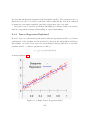
8 ADEP Example: Regression Analysis
8.1 What is Regression Analysis? . . . . . . . . . . . . . . . . . . . . . . .
8.1.1 Regression Explained . . . . . . . . . . . . . . . . . . . . . . . .
8.1.2 Linear Regression Explained . . . . . . . . . . . . . . . . . . . .
8.2 A Simple Linear Regression Example . . . . . . . . . . . . . . . . . . .
8.2.1 Least Squares Method . . . . . . . . . . . . . . . . . . . . . . .
8.2.2 Weighted Least Squares Method . . . . . . . . . . . . . . . . . .
8.3 Simple Linear Regression using ADEP Generated algorithm with Binary
Solution Representation . . . . . . . . . . . . . . . . . . . . . . . . . .
8.3.1 Represent Simple Least Squares Solution using Binary String . .
8.3.2 Define the Objective Function for Simple Linear Regression . . .
8.3.3 Generate HGA with Binary Representation using ADEP . . . .
8.3.4 Create and Save sample data in Excel . . . . . . . . . . . . . . .
8.3.5 Modify problem.xml . . . . . . . . . . . . . . . . . . . . . . . .
8.3.6 Modify Problem<T>::readInput() method in Problem.h . . . .
8.3.7 Modify Problem<T>::_evaluate() . . . . . . . . . . . . . . . . .
8.3.8 Override Problem_Base<T>::interpret() in Problem<T> . . .
8.3.9 Configure Binary Hybrid GA to improve algorithm performance
8.4 Simple Linear Regression using ADEP Generated algorithm with Continuous Solution Representation . . . . . . . . . . . . . . . . . . . . . .
8.4.1 Represent Simple Least Squares Solution using Floating Point
String . . . . . . . . . . . . . . . . . . . . . . . . . . . . . . . .
8.4.2 Define the Objective Function for Simple Linear Regression . . .
8.4.3 Generate HGA with Floating Point String Representation using
ADEP . . . . . . . . . . . . . . . . . . . . . . . . . . . . . . . .
8.4.4 Create and Save sample data in Excel . . . . . . . . . . . . . . .
8.4.5 Modify problem.xml . . . . . . . . . . . . . . . . . . . . . . . .
8.4.6 Modify Problem<T>::readInput() method in Problem.h . . . .
118
118
118
119
120
120
121
121
122
124
124
124
125
126
129
131
134
136
136
136
137
137
137
138
8.4.7
8.4.8
8.4.9
Modify UpperLowerBounds.xml file . . . . . . . . . . . . . . . . 138
Modify Problem<T>::_evaluate() . . . . . . . . . . . . . . . . 138
Override Problem_Base<T>::interpret() in Problem<T> . . . 140
9 ADEP Example: A Minimization Problem
142
List of Figures
143
List of Tables
147
Chapter 1
Getting Started
What you will learn in this chapter:
1. What ADEP is?
2. What Needs Does ADEP Fullfill?
3. What Features Does ADEP have?
4. Why Choose ADEP?
1.1
What ADEP is?
ADEP stands for Algorithm Development Environment for Problem solving. It is a
Problem Solving Environment (PSE) that allow user to configure and generate stateof-art meta-heuristic hybrid algorithms in C++ or Java source codes for solving various
real-life combinatorial and numerical optimization problems.
1.2
What Needs Does ADEP Fullfile?
To answer this questions, we must clarify what we mean by real-life combinatorial and
numerical optimization problems and what are meta-heuristic hybrid algorithms in 1.1
7
1.2.1
What Are Real-life Combinatorial and Numerical Optimization Problems?
Many real-life problems in industries and financial markets are essentially optimization
problems. Optimization refers to the study of problems in which one seeks to minimize
or maximize a real function by systematically choosing the values of real or integer
variables from within an allowed set. An optimization problem can be represented in
the following way
Given: a function f : A −→ R from some set A to the real numbers
Sought: an element x0 in A such that f (x0 ) ≤ f (x) for all x in A ("minimization")
or f (x0 ) ≥ f (x) for x all in A ("maximization").
Combinatorial optimization is a branch of optimization. Its domain is optimization problems where the set of feasible solutions is discrete or can be reduced to a
discrete one, and the goal is to find the best possible solution. Examples of combinatorial optimization include Quadratic Assignment Problem (QAP), Traveling Salesman
Problem (TSP), Vehicle Routing Problem (VRP), Hamiltonian Cycle Problem (HCP),
N-Queens Problem, Knapsack Problem and so on.
Numerical optimization is another branch of optimization. Its domain is optimization problems where the set of feasible solutions is continous or numerical values and
the goal is to find the best possible set of numerical values. Examples of numerical
optimization include linear and nonlinear regression analysis and so on
Each of those combinatorial and numerical problems can find numerous real-life
applications.
1.2.2
What Are Meta-heuristic Algorithms?
Many practical real-world combinatorial and numerical optimization problems tend
to be computationally intractable. they usually belong to the category of NP-hard
problem, implying they cannot be solved by exact method in tractable time period.
While advancement in computer technology is able to provide significant headway by
making available immense computing horsepower, it is far from being able to address
the needs of solving complex optimization problems. The challenge is really in the
algorithms front. Since traditional exact techniques such as branch and bound cannot
8
solve those problems in tractable time, heuristic algorithms were developed to look for
solution with good enough quality and find those solutions within short period of time.
however those heuristics usually suffered from the tendency of being trapped in the
local optimima and their performance become highly unreliable. As a results, in recent
years many highly effective meta-heuristic algorithms were developed that incorporate
mechanism to help the algorithm to escape from local optimia. this branch of algorithms include evolutionary algorithms, simulated annealing, tabu search, ant colony
optimization and neural networks have surfaced as viable stochastic optimization techniques.
1.2.3
ADEP Allow Users To Design and Implement Complex
and Effective Meta-heuristic Algorithms
With these basic understanding of real-life optimization problems and meta-heuristic
algorithms, let’s examine what needs does ADEP fullfill.
The state of the art research on meta-heuristic algorithms has made significant advancement in the last two decades. This coupled with the technological advancement in
computational horsepower have opened up avenues to explore problems of complexity
level that were previously considered insurmountable. In this regards, rapid design and
development of meta-heuristic algorithms has become an important and challenging
issue. The current meta-heuristic algorithm development methodology usually requires
significant effort in codes generation and modifications. As a result, the quality of the
meta-heuristic algorithm that solves a NP hard problem may be far from optimal in
terms of performance. This is likely due to the fact that the designer may not have the
resources or resolve to fine tune the algorithm. It is also likely that the programmer
may not possess the necessary experience and knowledge on meta-heuristics algorithms
to effectively make the necessary improvement.
ADEP was developed to address the need for rapid generation of efficient algorithms that target the real-life problems. the user only needs to modify the objective
function to convert the codes for solving the target problem. As a result, the time
to implement the bulk of codes for the HGA operators such as crossover, mutation,
parents selection, fitness scaling, population update, etc. can be devoted to other more
productive solution integration tasks. ADEP allows users to focus on the high-level
9
problem abstraction, significantly reduces the algorithm development time and effort
in designing and implementing the meta-heuristic algorithm to solve the problem.
1.2.4
ADEP Allow Users To Configure An Algorithms’ Performance towards On a Particular Problem
One of the main issues faced by system developers of meta-heuristic algorithms is that
there seem to be no "one size fits all" type of search algorithms. In other words, for
any given meta-heuristic algorithm with a particular parametric setting, it is unlikely
that it will perform equally well for all the problems of the same class. Hence, it is
common to mix and match between metaheuristics, or at least one metaheuristic and
one local search technique. It has also become a norm in algorithms development to
mix and match between the various available techniques to develop algorithms that
are able to capitalize on the strengths and merits of the various techniques. This has
also given rise to a group of algorithms known as memetic algorithm.
To configure a meta-heuristic algorithm to improve its performance on a problem,
it usually involves tremendous amount of time in inventing new algorithm operators
as well as testing the those operators by embedding them back in the algorithm. The
process of configuring such hybrid algorithms can be made easier if there is a computational platform to facilitate the algorithm design process. Thus ADEP comes in
handily in helping the users to design and configure highly efficient algorithm on a
problem by making numerous configuration options available (so that the user does
not need to reinvent the wheels and focus on the high level of designing and configuring
the algorithm).
ADEP makes the algoritm configuration process a much easier task by making the
following features available:
1. prev-written modules and algorithm operators that the user can easily add or
remove from the algorithm in designed by a few click of mouse
2. different parameters tunable in the algorithm can be fine tuned through ADEP
GUI
3. built-in compiler to compile and run the configured algorithm within the ADEP
10
environment that relieve the user the copy and replacement manual operation
during the numerous algorthm testing
4. charts and algorithm performance stastics displayed once the configured algorithm complete its run
5. automatic configuration engine for automatic algorithm configuration to be discussed in 1.2.5
1.2.5
ADEP Can Automatically configure algorithms
The increasing complexity of both problems and algorithms makes algorithm development and problem-solving more and more challenging. Conventional algorithm
development methodology usually requires significant effort in codes generation and
modifications. Furthermore, the quality of the algorithm depends very much on the
designer’s experience, level of knowledge specific to the problem being addressed, as
well as the algorithm flow stucture. A programmer without profound algorithm design
experience will find developing an effective and robust algorithm extremely challenging.
Not to mention that in practical scenarios, users may face with various requirements
of the algorithm. An algorithm that solves one particular class of problems well may
not work for other classes of problems or scenarios at all. This makes the algorithm
development for complex real-life applications even tougher.
ADEP can take over the user’s task of configure an algorithm to make it efficient to
solving the problem at hand. This was realized by the automatic algorithm configuration engine in ADEP. by using this engine, the user only need to specify the objective
function of the problem, and the algorithm take over the task of algorithm configuration to automatically look for algorithm configurations that achieve the optimum
performance.
It can be seen that with ADEP, the highly complicated and tedious process of
algorithm design and implementation as well as configuration is almost taken over by
the PSE. this makes the process of solving complex real-life problem an almost RAD
(Rapid Application Development) process, even for people who are not experienced
problem domain expert or experienced programmers.
11
1.3
What Features Does ADEP Have?
Some of those features have been briefly mentioned in 1.2.4 and 1.2.5, there are numerous available features in ADEP to help the user design and implement as well as
test run algorithms, some of the main features are listed below and illustrated in the
subsequent chapters
1.3.1
Intuitive GUI
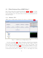
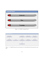
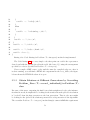
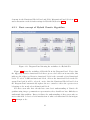
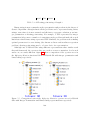
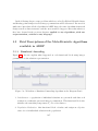
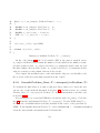
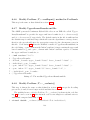
ADEP features a highly intuitive Graphical User Interface as illustrated in 1.1
Figure 1.1: ADEP Features A Highly Intuitive GUI
As can be seen in figure 1.1, a Memetic Algorithm (or Hybrid Genetic Algorithm
as it was previously known) is represented as a flow chart that consists of blocks of
function unit of the algorithm. this represents the control of the algorithm. when
one of the block is selected (in figure 1.1, the block "Stopping Condition" is selected),
the tree control below the algorithm flow chart displays the various options available
in this functional block what are configurable. The tree control display the various
12
operators that reside in the functional block and are organized into the tree structure
to indicate their execution sequence and relationships. the value and selection of those
operators can be easily accessed or updated by double-clicking the node that represent
the operator.
In the Command Panel at the top right corner of the application GUI, there are
three buttons "Generate" (to generate codes), "Run", (to run the configured algorithm), "Learning" (to invoke the automatic configuration engine to learn the problem
and configure the algorithm for the problem), the caption of which indicate the three
main functions of ADEP.
Below the Command Panel is the Algorithm Panel, in which there is a button
whose caption reads "Hybrid GA", indicating the current configuration is for a Hybrid
Genetic Algorithm. the bottom right panel next to the tree control always display
updated information about the selected node in the tree control.
The intuitive GUI allow an user with some fundamental understanding of an algorithm to quickly figure what each parts of the algorithm accomplish and behave and
quickly reduces the learning curve of the software
1.3.2
Automatic Generation of Source Codes
ADEP can generate highly efficient and complex algorithm complete complete project
files in VC6 and VC2005 as well as makefile, with just one click of button, by clicking
the "Generate" button on the Command Panel, the source codes generated can be
in any language (due to the way ADEP was designed) with current ADEP version
supporting the generation of C++ and Java source codes. the source codes generated
share highly similar framework albeit the languages of implementation are different.
and the codes were tested numerous times for cross platform compatibility so that they
are run on machines with different platform and operating systems.
1.3.3
Highly extensible algorithm framework
ADEP has a highly extensible algorithm framework, it incorporates a 3 layer architecture in which the actually code implementation is hidden by layer of XML database,
the XML data is a distributed tree structure file system consisting of many XML files
linked by execution order and relationship defined as rules in the ADEP environment,
13
ADEP environment communicate directly with the XML database layer but without
knowing where the actually source codes are located and not even aware which language
the source codes are written, XML database layer acts as a glue between many different subsystem, such as the compiler-driven subsystem, the source codes, the ADEP
environment. this makes the ADEP environment highly adaptable and extensible. To
include a new module for algorithm or algorithm operators into the ADEP framework
is as simple as copy the source code module into a folder and insert an XML file (with
links to that source code) into appropriate hierarchy of the file system. when the next
time the ADEP is started, the new code module will automatically be available.
because of this, an entire new branch of algorithms written in different languages
can be easily incorporated into ADEP without recompiling the ADEP source codes. In
fact, the ADEP environment was originally developed for Hybrid Genetic Algorithm
in C++, but due to its extensible nature of its architecture, other algorithms such as
Tabu Search, ACO and so on are added, and even in a different language Java.
The high extensibility of ADEP framework is also manifest in its source code framework, it is designed such that a user-defined objective function source code can be used
by any algorithm in its algorithm framework database, as long as they share the same
representation.
1.3.4
ADEP Has Built-in C++ Compilers
ADEP has its own built-in compilers, this means the user of ADEP does not need
to purchase another IDE such as Microsoft Visual Studio or Borland C++ Builder,
when the user generate the C++ source codes by clicking the "Generate" button on
the Command Panel, a batch file containing the compilation scripts is also generated
in the same folder where the generated source codes reside. To compile the source,
simply double clicking the batch file (if the user is using Windows as the OS) or copy
and paste the content in the batch file to the command line of the console (if the user
is using other OS) and press ENTER. an executable file will be generated as the batch
file calls the embedded compiler in ADEP.
14
1.3.5
ADEP Has Built-in Java Compiler
ADEP also has built in java compiler, so that user do not need to install Java SDK or
Java runtime in order to compile and run the ADEP generated java source codes. the
ADEP built-in java compiler automatically compile the java source code into executable
file (this also make the execution of the algorithm faster now that the source code is
compiled or native machine code instead of java bytecode). indeed ADEP compilerdriver architecture to be described in the later chapters allow incorporation of any type
of compiler for any language into ADEP without the need to modify the source code of
ADEP, which makes the system highly extensible for incorporating other programming
languages.
1.3.6
ADEP allow configured algorithm to test run in the ADEP
ADEP allow user to upload their objective function in the problem solving environment
and directly run a configured algorithm with that objective function without leaving the
environment. This feature might seen trivial in the first place. but without this feature,
the task of test running algorithms for fine-tuning and configuration can be daunting.
imagine that the user is adjusting a particular parameter for 10 different values, without
using this feature, the user has to generate the code from the current configuration,
replace the default objective function with the problem-specific objective function,
and then compile and run the source codes, after that try to record the different
performance statistics. now that since the problem the user is trying to solve requires
a lot of paramter tunning, say that the user will have try to change around 20 different
operators and parameters in order to obtain the desire configuration. The repeated
non-brain-involved process may finally kill the user’s very creative brain cells or lead to
the user having an enhanced vision of quiting his job. On the other hand, having this
"Run" feature, the user can just upload his objective function to the environment, click
the button "Run" which automatically compile the algorithm with the user’s uploaded
objective function and other information, run the compiled algorithm and report the
performance measures nicely in table format and chart figure which the user can then
save, all being done by only the clicking of "Run" button
15
1.3.7
ADEP can replace the task of looking for the best configured algorithm on the problem
as mentioned in 1.3.6, the process of configuring algorithm can be daunting, even with
the "Run" feature, especially for a new problem for which approach to obtain the
best configuration is unknown (since the user cannot tell whether the configuration he
obtained so far is good enough). In such a situation, the automatic configuration engine
become extremely useful, the process of preparing is also extremely easy and almost
identical to that of the "Run" feature in 1.3.6, the user upload the objective function,
then click "Learn" button on the Command Panel, the automatic configuration engine
is exported to a user specified folder and in there it is compiled and run. No more
user interaction is required, the automatic configuration engine periodically look for
promising configuration and save them to files. the user can leave the configuration
engine to run on its own and only come back later to collect the best configuration
found by the engine. those configuration files can then be converted back to source
code by ADEP.
instead of performing a brute force searching for best configuration (which will
be next to impossible since the sheer number of possible configuration and the time
taken to test run each configurable), the automatic configuration engine makes use of
meta-heuristic machine learning algorithm to perform intelligent search for the best
configuration.
the automatic configuration engine is generated entirely in C++ source codes by
ADEP and then compiled and set to run. this is highly advantageous. Firstly, the
engine is written in C++ source codes that is platform independent, therefore, the
whole engine can be brought to another machine to run, regardless of the OS running
on that machine. Secondly, even when the engine is running on the same machine
as the ADEP, the ADEP can perform other tasks at the time the engine is running
without any delay or application hanging issues, since the engine and ADEP are now
run as two totally independent processes on the same machine. Thirdly, the engine is
exported by ADEP as C++ source codes, the user can modify the engine to suit his
need if that is necessary.
16
1.3.8
Other Features of ADEP
Apart from those features listed above, ADEP has many other features such as saving configured algorithms (not as source codes but as configuration file that can be
loaded back into ADEP), print current configuration, extend different algorithm frameworks by adding in new operators, view list of configurable parameters and operators,
extensive instruction and information knowledge for various operators, programming
language extension and so on.
1.4
Why Choose ADEP?
So ADEP is another PSE to be use for meta-heuristic algorithms on optimization
problem, you may say, and nowaday there is abundant libaries and package that does
this job, and even MATLab has one too, then why should I choose ADEP? Well,
You should choose ADEP because ADEP does this job...MUCH better than other
available libaries. there are many reasons, some of which can be seen as that ADEP
combine many benefits and advantages of those available packages, other can be seen
as useful feasible only available in ADEP.
First of all, all any of those PSE and package are as extensible as ADEP itself. The
3 tier structure makes the system high extensible from many different aspects such as
compiler installation, language installation, algorithm installation.
Many libraries such as GALib are just libraries, and are basically only useful for
Genetic Algorithm algorithm expert with some intermediate level of programming
skill and have been spending some time to study the document of the library. they
do not have the fancy look of the intuitive GUI of ADEP, cannot perform run test,
and automatically generate statistics, does not have automatic configuration engine.
moreover, when a libary whose name read like GALib, you know that they won’t
include other meta-heuristics algorithm such as Simulated Annealing, Tabu Search, or
ACO.
Other PSE such as TOMLAB (optimization PSE of MATLAB) or HEEDS (stands
for Hierarchical Evolutionary Engineering Design System), although incorporating various optimization techniques, including genetic algorithm (GA) and with user-friendly
interface for exploring various optimization tools for solving a myriad of optimization
17
problems being addressed. Those environements are essentially simulation environments. Though various algorithms can be configured and executed efficiently in these
environments, the execution depends on the entire system. For many applications
which require embedded real-time solver, this class of environments does not offer
the flexibility to configure an efficient stand-alone program, albeit a turnkey problemsolving algorithm. Moreover, PSE like TOMLAB require expensive third party software such as MATLab.
Other PSE was developed in Java, with nice facilities to output test run results
and performance statistics, but they were also designed mostly with simulation in
mind, with little freedom for configuring efficient stand-alone program. ADEP has the
freedom to generate C++ source codes whenever it needs, and even its java code can
be compiled into executable. moreover, the automatic configuration engine is rarely
offered by any other PSEs available. the source codes generated by ADEP are totally
decoupled from the ADEP environment whereas many Java GA PSE requires its own
presence as well as the Java Virtual Machine to run.
ADEP - generated source codes and the generate automatic configuration engine
are highly portable, which makes ADEP virtually cross-platform. the source codes
framework were designed using Design Patterns making them highly structured. From
the above discussion we can also see than many of the useful features available in
ADEP as discussed in 1.3 are not available in other meta-heurist PSE or software
package currently available. This makes ADEP stands out from those other software
packages.
18
Chapter 2
Installing ADEP
This chapter you will learn
1. How to set up ADEP in your computer
2. How to register your copy of ADEP
2.1
Launch ADEP Installer
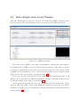
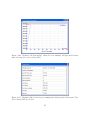
The ADEP setup file is available as a Windows installer. To install ADEP in your
computer, launch the ADEP Windows installer. The following figure is the screen shot
of the installer program after it is launched:
Click "Next" to proceed
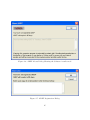
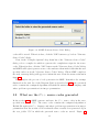
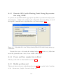
2.2
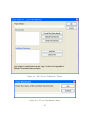
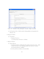
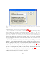
Enter ADEP Installer Password
The figure 2.2 shows the next screen of the installer that appear
Figure 2.2 asks the user to enter the ADEP installer password, the default password
is "adep" (or it might be specified otherwise by the software distributor from whom
the user can obtain the installer password).
Enter the installer password then press "Next"
19
Figure 2.1: ADEP Installer Screen Shot After Launch
20
Figure 2.2: Enter installer password
21
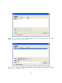
Figure 2.3: Select a directory to install ADEP
2.3
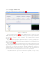
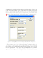
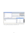
Select a Directory for Installation
In the next screen 2.3 , the user is asked to select a directory for installation, the
default is "C:\ Program Files\ ADEP"
Select the target directory or use the default installation directory, and press
"Next". At this point, the installer begin to install the ADEP files to the selected
directory, as illustrated in figure 2.4
In subsequent screens, the users are asked the options to create desktop and quick
launch short cuts. After the user make his prefered selections and press "Next", the
installation is completed.
22
Figure 2.4: ADEP Installation in Progress
23
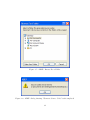
2.4
Enter Registration Serial Number
After the installation is completed, the user can launch the ADEP application from
the Start menu. The following figure is the screen shot of the ADEP on launch.
Figure 2.5: ADEP on Launch
The full license of ADEP comes with a serial number, without this serial number,
the full function of ADEP is only provided for the first 90 days. After this period, the
user need to purchase the license in order to enjoy its function. The current license
of ADEP after its installation can be view in the About dialog by selecting the menu
Help→About. The About dialog is shown in figure 2.6
If the user already purchased the licence and has the serial number, the serial
number can be entered by selecting the menu Help→Register. After the menu selection,
the Register dialog appeared as seen in figure 2.7
In the registration dialog, the user can copy and paste the serial number in the
text box and press "OK". If the serial number is entered correctly, the user will be
informed about the success of registration. and the About dialog after registration is
shown in figure 2.8
24
Figure 2.6: ADEP About Dialog Showing the Software is unlicenced
Figure 2.7: ADEP Registration Dialog
25
Figure 2.8: ADEP About Dialog Showing the Software is now Licenced
26
Chapter 3
Generate and Compile ADEP Source
Codes
In this chapter, you will learn
1. How to use ADEP to generate C++ source codes
2. What are the C++ source codes generated
3. Understand the process involved in solving an optimization problem
4. How to modify the generated C++ source codes to solve the optimization problem
5. How to obtain the solution output form the ADEP generated algorithm for use
To allow you to have a better understanding of the last two topics, we will show you
an real-life problem-solving example using the generated code. Section 3.3.2 describe
the 8-Queens problem which is a real life combinatorial problem — the 8-Queens
Problem
3.1
How to Use ADEP to Generate C++ Source Codes
Before we go into the tutorial on how to use ADEP to generate C++ source codes, let
us be familiarized with the ADEP GUI.
27
3.1.1
Explain ADEP GUI
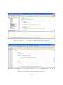
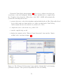
Launch the ADEP application as shown in figure 3.1.
Figure 3.1: ADEP GUI
As was explained in Section1.3.1 about the ADEP GUI, the top right corner of the
ADEP GUI features the Command Panel, which hosts the three main commands of
the application: "Generate", "Run", "Learning". The Command Panel is shown in
the figure 3.2.
The default loaded algorithm is Hybrid GA which is a memetic algorithm framework. The work flow of the Hybrid GA framework displayed by the Diagram Panel as
illustrated in figure 3.3
Notice that at the title bar of the Diagram Panel, three different information about
the current loaded algorithm framework are displayed: the algorithm framework name
("Hybrid GA"), the problem representation ("[Integer Permutation]"), and the programming language for the generated source codes ("[cpp]"). The 3 informations displayed in the title bar in the Diagram Panel deserves some explanations:
1. algorithm framework: typical for meta-heuristics algorithm, each type of algo28
Figure 3.2: ADEP Command Panel
Figure 3.3: ADEP Diagram Panel showing the default Hybrid GA framework work
flow
29
rithm usually has numerous different configuration consisting of a wide variety
of parameters and opertors. those configurations all together for the algorithm
framework for a particular branch of the algorithm
2. problem representation: in meta-heuristic algorithms, a candidate solution generated by the algorithm is usually represented in some form of symbols, this is
known as the problem’s representation. for example, in the Travelling Salesman
Problem (TSP), the TSP candidate solution solution is usually represented by an
integer permutation in which each integer is unique and represent the city which
the salesman travel in sequence. this representation is the "Integer Permutation"
representation.
3. programming language: any algorithm can be written in a number of high level
programming language, the programming language indicated in the title bar of
Diagram Panel simply indicate to the user that the source code generated for the
Hybrid GA would be in C++ ("[cpp]") language
The panel directly below the Command Panel is known as Algorithm Panel, it is
through the command in this panel that the user can switch between different algorithm
frameworks as well as problem representation and the programming language of the
generated source codes. The panel directly below the Diagram Panel is the Functional
Block Panel which display a tree representing various options available for a selected
functional block of the algorithm framework as displayed in the Diagram Panel. To
the right of the Functional Block Panel is the Operator Node Panel which display the
information pertaining to the information about the selected node in the tree control
of the Functional Block Panel. These features will be further explained in the chapter
that discuss about how to configure the ADEP generated algorithm.
3.1.2
Generate Source Codes
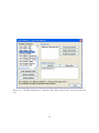
To generate the source codes from ADEP, click the "Generate" button in the Command
Panel, the "Generate Source Code" dialog appeared as shown in figure 3.4
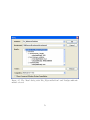
In the "Generate Source Codes" dialog as shown in figure 3.4, click the "Browse"
button and the "Browse for a folder" dialog will pop up, as shown in figure 3.5. In the
"Browse for a folder" dialog, select or create a folder into which the generated source
30
Figure 3.4: ADEP Generate Source Code Dialog
codes will be stored. When it is done, click the "OK" button to go back to "Generate
Source Codes" dialog.
Next, in the "Compiler Options" drop down list of the "Generate Source Codes"
dialog, select a compiler for which to generate the compilation scripts for the source
codes. When it is done, click the "OK" button on the "Generate Source Codes" dialog
and ADEP will begin to generate source codes and store them in the folder that the user
specified earlier on in the "Generate Source Codes" dialog. When ADEP completes
the task, a message dialog will appear to inform the user about the status as shown in
figure 3.6
This complete the process of code generation in ADEP. Remember the settings
displayed at the title bar of the Diagram Panel as described in 3.1.1, the generated
source contains the configured algorithm of Hybrid GA written in C++ language and
whose problem representation is in integer permutation.
3.2
What are the C++ source codes generated
In the section 3.1.2, ADEP generate and store the C++ source codes in the userspecified root_folder "C1". The source codes contains the configured algorithm of
Hybrid GA written in C++ language and whose problem representation is in integer
permutation.Now Let us take a look at what files have actually been generated. Open
the root_folder "C1" in which the generated source codes are stored. Figure 3.7
31
Figure 3.5: ADEP: Browse For a Folder
Figure 3.6: ADEP: dialog showing "Generate Source Code" task completed
32
illustrate the files and folders contained inside root_folder "C1".
Figure 3.7: The list of folders and files generated by ADEP in the root_folder "C1"
We will now explain what those folders and files are about in figure 3.7.
1. adep.dsw, adep.dsp: these are the Visual C++ 6.0 workspace and project files.
they can be used to modify and compile the ADEP generated source codes in
Visual Studio 6.0
2. adep.sln, adep.vcproj: these are the Visual C++ 2005 workspace and project
files. they can be used to modify and compile the ADEP generated source codes
in the Visual Studio 2005
3. makefile: the make file can be used on other OS to compile the ADEP generated
source codes
4. compile.bat: this is a batch file that contains the compilation scripts to compile
the ADEP generated source codes. The reason that this file is generated is for
33
the user who does not have any compiler installed in his computer (in this case,
none of the adep.dsw, adep.sln, or makefile is of usage). Since ADEP comes
with built-in compilers, the compile.bat simply invokes a user-specified built-in
compiler(remember the steps performed in the "Generate Source Codes" dialog
in section 3.1.2) to compile the source codes after the user add in the problem
specific evaluation function into the source code.
5. problem.xml: this is an xml file that contains the specified XML configuration
settings for a problem instance. By default, three information about the problem
instance is contained in this file: chromosome length, search direction, and best
known solution found in the past. The details of this file will be further explained
in section 3.4
6. the rest of them are folders that contains the source codes generated by ADEP,
the generated source codes are nicely separated into different modules (that is,
folders) according to their functions. For examples, the "csv_doc" folder contains
the C++ class file that can read in a specific Excel file of the "comma separated
values" file format, on the other hand, "tinyxml" folder contains the C++ class
files that can parse and write XML files.
3.3
Understand 8-Queens Problem and How it can
be solved as an optimization Problem
Before we rush into modifying the source codes, we need to understand the paradigm
in problem solving for optimization problem. To facilitate the understanding on how
to solve optimization, the 8-Queens optimization problem is taken as an example and
illustrated in the subsequent sections.
3.3.1
How to Solve an optimization problem effectively
To learn the approach on how to solve an optimization problem, follow the steps below
1. Understand the problem and its constraints (refer to 3.3.2)
34
2. Understand how to formulate the problem solution using a particular representation (refer to 3.3.3)
3. Understand how to define the objective function (refer to 3.3.4)
4. The rest of the steps is just to write the algorithm to solve the problem by making
use of the objective function and the representation
3.3.2
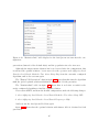
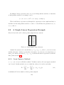
What is The 8 Queens Problem and What are its constraints?
The eight queens puzzle is the problem of putting eight chess queens on an 8 × 8
chessboard such that none of them is able to capture any other using the standard
chess queen’s moves. The queens must be placed in such a way that no two queens
would be able to attack each other. Thus, a solution requires that no two queens share
the same row, column, or diagonal. The eight queens puzzle is an example of the more
general n queens puzzle of placing n queens on an n × n chessboard, where solutions
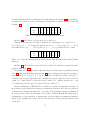
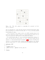
exist only for n = 1 and n ≥ 4. figure 3.8 demonstrate one of the possible solution for
8 Queens Problem.
The puzzle was originally proposed in 1848 by the chess player Max Bezzel and
appeared in the popular early 1990s computer game The 7th Guest. The problem can
be quite computationally expensive as there are 283,274,583,552 (64x63x..x58x57/8!)
possible arrangements, but only 92 solutions. Therefore it is computationally very
expensive to use brute force computational technique. This is exactly the type of
problem where meta-heuristic algorithm such as Hybrid GA can obtain high quality
solution within relatively short period of time.
3.3.3
How to Formulate 8 Queens Problem Solution as Integer
Permutation Problem?
Before we go into the details of formulation, we will try to explain what is a permutation
for those users who do not have any background on combinatorial optimization. In
combinatorial optimization, a permutation is usually understood to be a sequence
containing each element from a finite set once, and only once. The concept of sequence
35
Figure 3.8: A 8 Queens Solution
is distinct from that of a set, in that the elements of a sequence appear in some order:
the sequence has a first element (unless it is empty), a second element (unless its length
is less than 2), and so on. In contrast, the elements in a set have no order; {1, 2, 3}
and {3, 2, 1} are different ways to denote the same set.
In the Hybrid GA source codes, the values in integer permutation usually has a
range with minimum value being 0 and maximum value being n-1 (where n is the length
of the permutation. therefore some examples of an integer permutation of length 4 will
be {0, 1, 2, 3}, {3, 1, 2, 0} and {2, 1, 0, 3} and so on. the particular reason that
it starts with zero is because in most of high level programming language, an array
usually start with 0.
Now that you understand what is an integer permutation, we will define some
syntax for integer permutation here suppose an integer permutation x̄={5, 3, 4, 2, 1,
0}. then length(x̄)=6 is defined as the length of the permutation x̄, and x̄(0)=5 and
x̄(2)=4 indicate that the value at the 0-th index of x̄ is 5 while the value at the 2-th
index of x̄ is 4.
The 8-Queens problem solution can be easily represented by an integer permutation,
36
we will demonstrate how to transform the solution displayed in figure 3.8 into an integer
permutation. below is a table showing the arrangement of quenes on the chessboard
in figure 3.8.
Queens
row
col
1
1
f
2
2
a
3
3
e
4 5 6
4 5 6
b h c
7
7
g
8
8
d
Table 3.1: 8 Queens Arrangement in Chess Board
In table 3.1, the Queen 1 is placed in row 1 and col f.
Now since the Queens, row and col symbols are all arbitrary, we can use {0, 1, ...,
7} to replace {1, ...., 8} for Queens symbol; use {0, 1, ..., 7} to replace {1, ...., 8} for
row symbols;use {0, 1, ... , 7} to replace {a, b, c, ..., h, g}, and the table becomes
Queens
row
col
0
0
5
1
1
0
2
2
4
3
3
1
4
4
6
5
5
2
6
6
7
7
7
3
Table 3.2: 8 Queens Arrangement in Chess Board with Redefined Row and Column
Symbols
In table 3.2, the Queen 0 is placed in row 0 and col 5, which is actually the same
position as in table 3.1.
Observant users at this point would have discovered the integer permutation from
table 3.2. The Queen arrangement in table 3.2 can be simply represented by an integer
permutation x̄={5, 0, 4, 1, 6, 2, 7, 3}. To illustrate how this is possible, take x̄(0)=5
and x̄(1)=0, these two equations can be translated to mean "Queen 0 is placed at row
0 and col 5" and "Queen 1 is placed at row 1 and col 0". And in generate x̄r=c can
be translated to mean "Queen r is placed at row r and col c".
In the terminology of Hybrid GA, a solution is called a chromosome, therefore if
the solution is represented as an integer permutation x̄, then we will called a solution x̄
a chromosome, and in expression x̄(i)=v we will call i (an index of integer permutation
x̄) as locus and j (value at i-th index of x̄) as allae. Thus in Hybrid GA using integer
permutation as representation, a chromosome is just an integer permutation with the
index of the permutation being called locus and value at the particular index begin
called allae.
37
3.3.4
How to Define an Objective Value for a 8-Queens Problem Solution?
Now the formulation of 8-Queens problem solution as a Hybrid GA chromosome in
the form of integer permutation has been described, we need an objective function to
define a objective value for each chromosome.
But first of all, what is meant by an objective value? for the sake of those users
who do not have background in optimization, an objective value can be understood as
the quality of a solution. An objective function is therefore a function that measure
the quality of a solution and then assign it an objective value. As defined in 1.2.1, an
optimization problem is to look for a solution whose objective value is maximum or
minimum.
For some problem the objective value can be defined as the cost, for example, in a
travelling salesman problem, a solution will be the sequences of cities that the traveling
salesman visits in order. and the objective value can be define to be the cost of traveling
all the cities using the sequences of cities indicated by the solution, which can simply
mean the total distance travelled when the traveling salesman visit each city according
to the tour sequency indicated by the solution. For this type of objective value that
stands for a cost, the purpose of the meta-heuristic is therefore to look for a solution
that has minimum cost, that is, the objective of the meta-heuristic algorithm is to look
for a solution that has a minimum objective value as defined by the cost.
For some other problems, the objective value can be defined as the gain, for example,
In the Halmitonion Cycle Problem, a solution is tour travelled by an agent such that
each city is visited by the agent once and only once and the last cities reached by
the agent is the first city that the agent left for the tour. For this kind of problem,
the objective value of the solution is defined by the total number of cities that can be
included in the Halmitonian cycle toured by the agent. Then the problem becomes the
search for a solution that has a maximum objective value as defined by the gain (the
total number of cities included in the Halmitonian cycle).
From the above analysis, in optimization, an objective function can be defined such
that the search is for maximization or for minimization. Therefore, before we start to
define the objective function for the 8-Queens Problem, we need to decide whether the
algorithm is a maximization or a minimization search.
38
for the 8-Queens problem, there are three constraints: any two queens cannot be on
the same row, or same column, or same diagonal. the chromosome representation as integer permutation has removed the first two constraints (since the integer permutation
automatically ensures that no two queens will be in the same row or same column).
then to determine quality of a solution is to determine how many not-in-same-diagonal
constraints violation are created or removed by the solution. if the objective value is
defined as the total number of not-in-same-diagonal constraints violation are created,
the search will be minimization(to minimize the total number of not-in-same-diagonal
constraints violation created). if the objective value is defined as the total number of
not-in-same-diagonal constraints violations are removed by the solution, the search will
be maximization (to maximize the total number of not-in-same-diagonal constraints
violations removed).
if we decide to use maximization search, that is, the objective value of a solution
is defined as the total number of not-in-same-diagonal constraints violation created by
the solution, we can define the objective function as follows:
f (~x) =
N
−2 N
−1
X
X
conf lict_removed(i, j)
(3.1)
1 |rowi − rowj | =
6 |~x[rowi ] − ~x[rowj ]|;
0 otherwise
(3.2)
i=0 j=i+1
where
(
conf lict_removed(rowi , rowj ) =
The equation 3.2 defines a function conf lict_removed(i, j) which return 1 if the
queen at row i and the queen at row j are not on the same diagonal and return 0
otherwise. the statement |rowi − rowj | 6= |~x[rowi ] − ~x[rowj ]| simply means that the
Queen occupying row i is not in the same diagonal as the Queen occupying row j.
The objective function f (~x) defined in equation 3.1 is the total number of not-insame-daigonal constraint conflicts removed. N is the total number of queens (which is
8 for 8-Queens problem). and ~x[rowi ] is the column index for the queen at row i.
39
3.4
How to modify the generated C++ source codes
to solve 8-Queens Problem
This Section will explain how to add the problem objective function to the ADEP
generated source codes so that the generated algorithm can actually solve a problem.
The following steps are taken:
1. How to locate and open the source code files for modification
2. How to understand and modify the source code to solve a problem
3.4.1
How to Locate and Open the Problem.h File
To add the objective function to the generate source codes, the class to which the
objective function is to be added should be located, this class is stored in the Problem.h file. The following paragraph explains where to locate the Problem.h file in the
root_folder "C1"
Assume that you have VC 6.0 (or VC 2005) installed in your computer, double click
adep.dsw (or adep.sln) workspace file to open the ADEP generated project. After VC
6 is launched, switch to the "FileView" in the Workspace of the studio, navigate to
the "problem" folder in the "FileView" panel, open the folder and double click the
"Problem.h" file listed in the folder. At this time, the "Problem.h" will be loaded and
display in the studio editor windows as shown in figure 3.9
For user that use VC 2005, similar steps can be taken to load the Problem.h file
into the editor panel.
If you do not have any of those IDEs, you can still access and modify the Problem.h
file, by navigating to the folder "problem" in root_folder "C1", and open the Problem.h
file in the folder using your favorite editor. Figure 3.10 shows the Problem.h file opened
in notepad++.
ADEP source code files usually contains extensive comments to explain the various
features in the source codes, Problem.h is no exception. Ignore those comments, Problem.h essentially contains the definition of the class Problem<T> under the namespace
ADEP. In the Problem<T> declaration, apart from the constructor and destructor
method (which the user does not need to pay attention during most implementations),
40
Figure 3.9: Visual C++ 6 workspace with Problem.h file displayed
Figure 3.10: Problem.h file opened in notepad++
41
there are two method: readInput() and _evaluate(). The readInput() method is to initialize the problem specific data while the _evaluate() method is the default objective
function. The details of readInput() method and _evaluate() method are explained in
the comments as well as the accopany Code Library Help.chm document.
3.4.2
Understand problem.xml and Problem<T>::readInput()
method
Since we have understood the integer permutation representation for a solution in
N-Queens as well as how the objective function for 8-Queens can be defined. we
can implement the objective function in the Problem<T>::_evaluate() method. But
before we go into that there are algorithm configuration that we need to take care.
The following list the source code contained in the Problem<T>::readInput() of the
Problem.h file:
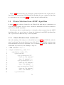
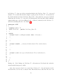
1 v i r t u a l bool r e a d I n p u t ( const char∗ f i l e n a m e )
2 {
3 XmlProblemReader r e a d e r ;
4
5 // r e a d e r l o a d d a t a from t h e xml f i l e
6
i f ( ! r e a d e r . loadXmlDoc ( f i l e n a m e ) )
7 {
8
debug << " f a i l e d ␣ t o ␣ l o a d ␣" << f i l e n a m e ;
9
debug . e n d l ( ) ;
10
11
return f a l s e ;
12 }
13
14 // r e a d e r a c t i o n #1
15
i f ( reader . isBestKnownSolutionAvailable ( ) )
16 {
17
this−>setBestKnownSolution ( r e a d e r . getBestKnownSolution ( ) ) ;
18 }
19 // r e a d e r a c t i o n #2
42
20
this−>setChromosomeLength ( r e a d e r . getChromosomeLength ( ) ) ;
21 // r e a d e r a c t i o n #3
22
this−>enableSearchForMaximum ( r e a d e r . isSearchForMaximum ( ) ) ;
23
24 //TODO: l o a d o t h e r d a t a from i n p u t f i l e s or do o t h e r
25 // i n i t i a l i z a t i o n h e r e
26
27 return true ;
28 }
Listing 3.1: Code Listing for ADEP generated Problem<T>::readInput() method
The source codes in 3.1 will be explained line by line here.
In line 1 of source codes 3.1, the virtual method readInput() is declared with a const
char* parameter which specifies a file name. This parameter is the problem.xml file
that is briefly described section 3.2. that means whatever information that is contained
in problem.xml file, we will make use of in the algorithm. Before we go on to describe
other source codes, Let’s take some time to understand problem.xml file first. below
shows the problem.xml file generated by ADEP:
1 <?xml version=" 1 . 0 " ?>
2 <problem name=" problem ">
3
4 <o v e r v i e w>
5
<chromosome_length v a l u e=" 15 " />
6
<best_known_solution e x i s t e d=" t r u e " v a l u e="0" />
7
<maximization v a l u e=" t r u e " />
8 </ o v e r v i e w>
9
10 <p a r a m e t e r s>
11
<param name="dummy1" v a l u e="0" type=" i n t " />
12
<param name="dummy2" v a l u e="0" type=" double " />
13
<param name="dummy3" v a l u e=" t r u e " type=" b o o l " />
14
<param name="dummy4" v a l u e=" f a l s e " type=" b o o l " />
15
<param name="dummy5" v a l u e="dummy" type=" s t r i n g " />
43
16 </ p a r a m e t e r s>
17
18 </ problem>
Listing 3.2: Code Listing for problem.xml
In the code listing of the problem.xml in 3.2, there are two sections, the "<overview>"
section contains the algorithm setting, while the "<parameters>" section specifies the
user-defined parameter to be loaded by reader in 3.1. For the moment, the "<parameters>" section can be ignored, "<overview>" section contains 3 critcal information
that is to be read by the algorithm: chromosome_length, best_known_solution, maximization. those parameters were explained in the comment of readInput() method in
the Problem.h file.
In line 3 of source codes 3.1, an object of class XmlProblemReader, reader, is
created. its loadXmlDoc() method is called in line 6 is called to load the data into
reader.
The statement below the comment //reader action #1 is executed to load in
the information about the best known solution found in the past. Only the objective value of best known solution found in past is of interest to us, this objective
value can be either a calculated value or obtained by some other algorithms in the
past. In a sense, the objective value of the best known solution can be thought of
as the global optimal value that we wish to reach. The information about the best
known solution found in the past is useful in the sense that if that information is available, the algorithm is able to terminate when it find this solution, if the algorithm
is configure to terminate in this way. This ensures that no extra CPU is wasted if
we already know the global optimal fitness value. If no such an objective value information is available (when reader.isBestKnownSolutionAvailable() return false, which
is resulted from the "<best_known_solution..." line in problem.xml being written as
"<best_known_solution existed="false" value="0""), the algorithm will continue to
search until other termination criteria reached.
The statement below the comment //reader action #2 is executed to set the
length of the chromosome used in the algorithm. (Remember from 3.3.3 that the
length of a chromosome is the length of the integer permutation in an algorithm using integer permutation as representation, for example, in 8-Queens, the chromosome
44
length will be 8). The reader object obtain the value of chromosome length from
"<chromosome_length..." statement in problem.xml.
The statement below the comment //reader action #3 is executed to set the
search direction of the algorithm. The reader object obtain the value of search direction
from "<maximization..." statement in problem.xml
In some cases, user might also want load in some other data from other sources,
readInput() method is a perfect place to start, because it is almost the first method
to be called by the algorithm. To put in user-define initialization code, just enter
them after the comment line "//TODO: load other data from input files or do other
initialization here".
This completes the analysis of the source codes in readInput(), basically, readInput
load the algorithm information from problem.xml file and used it to initialize parameters used in the algorithm. The advantages of loading algorithm settings from external
XML file is obvious when it comes to use the algorithm to solve another problem, for
example, instead of solving the 8-Queens problem, the algorithm is asked to solve the
9-Queens problem, the compiled source codes for 8-Queens problem does not need to
be modified and recompiled, all that is needed is to open the problem.xml file, and
edit the chromosome_length setting in the XML file. When this is done, run the previously compiled source code, and the correct solution will automatically be generated
for 9-Queens problem instead of 8-Queens problem.
Now we have gone through a detailed discussion about readInput() and problem.xml, let us start to work on the 8-Queens Problem. below is the modified problem.xml file for the 8-Queens Problem.
1 <?xml version=" 1 . 0 " ?>
2 <problem name="8−Queens ␣ Problem ">
3
4 <o v e r v i e w>
5
<chromosome_length v a l u e="8" />
6
<best_known_solution e x i s t e d=" t r u e " v a l u e=" 28 " />
7
<maximization v a l u e=" t r u e " />
8 </ o v e r v i e w>
9
10 <p a r a m e t e r s>
45
11 </ p a r a m e t e r s>
12
13 </ problem>
Listing 3.3: Code Listing for problem.xml prepared for 8-Queens Problem
In the problem.xml file prepared for 8-Queens Problem shown in 3.3, the best_known_solution
value is set to 28, this is the optimal objective value for 8-Queens problem, since the
= 28. maximaximum number of conflict violation that can be removed is 8×(8−1)
2
mization is set to true since we want the algorithm to search for a maximum objective
value. chromosome_length is set to 8 which is the integer permutation length for a
8-Queens solution. since the "<parameters>" section is not used in this case, their
dummy entries are removed.
The readInput() in the case of 8-Queens problem does not require any modification.
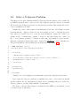
3.4.3
Understand _evaluate() method and How Objective Function Is Implemented in the Method
After the modification done in the problem.xml, we can add in the objective function
in to the Problem<T>::_evaluate() method in the Problem.h file.
Before we go into modifying the _evaluate() method, let us try to understand the
source codes generated in the _evaluate() by ADEP. Below is the code listing generated
by ADEP
1 v i r t u a l double _evaluate ( I n d i v i d u a l <T>& i n d i v i d u a l )
2 {
3 // a c t i o n #1
4 double o b j e c t i v e _ v a l u e = 0 . 0 ;
5 Chromosome<T>∗ pChrom=i n d i v i d u a l [ 0 ] ;
6
a s s e r t ( pChrom!=NULL ) ;
7 Chromosome<T>& chromosome=∗pChrom ;
8
9
a s s e r t ( ! chromosome . empty ( ) ) ;
10
11 // a c t i o n #2
46
12
int chromosomeLength=chromosome . s i z e ( ) ;
13
a s s e r t ( chromosomeLength<=this−>getChromosomeLength ( ) ) ;
14
15 //TODO: add c o d e s f o r f i t n e s s c a l c u l a t i o n h e r e
16
17 return o b j e c t i v e _ v a l u e ;
18 }
Listing 3.4: Code Listing for ADEP generated Problem<T>::_evaluate() method
In the code listing 3.4, there is a parameter that individual is passed into the
_evalate(), this parameter is an Individual<T> object which represents a solution
generated by Hybrid GA. The purpose of _evaluate() is to calculate an objective
value of the parameter individual and return the calculated objective value.
Earlier on in section 3.3.3 and 3.3.4, we have already written the pseudo code for
the objective function of 8-Queens. The first thing that we need to clarify is that in the
code listing 3.3.3, what is representing the integer permutation x̄ in the equation3.1.
To answer this question, let us start to analyze the code below the comment
// action #1, in this code, a local reference chromosome is created that is referenced
to the first Chromosome<T> object stored in individual. this reference chromosome
refer to the actual integer permutatin x̄ that we are interested in. In the source code
design of ADEP. ADEP algorithms have an Individual<T> object as a single solution,
each Individual<T> object may keep one or more copies of Chromosome<T> objects.
The reason that ADEP algorithms have the solution representation data structure in
this way is because for some algorithms, there might be chances that a solution cannot
be represented by a single Chromosome<T> object but need to be kept in multiple
Chromosome<T> objects. To ensure that such a case can be taken into account, the
Individual<T>←Chromosome<T> data structure is used so that an Individual<T>
object can represent a solution not matter how is the solution represented. In the
case of Hybrid GA with integer permutation representation, however, one Chromosome<T> object is sufficient to represent the entire integer permutation which is a
solution. Therefore in the ADEP generated code as listed in 3.4, the reference chromosome will be representing the integer permutation x̄ in the equation 3.1.
Let us now move to the source code below the comment //action #2 in the code
47
listing 3.4, a local variable chromosomeLength is created and assigned the value of
the size of chromosome. For the users who are wondering what value will be for 8Queens Problem, the variable chromosomeLength=8 in the case of 8-Queens Problem,
the ADEP generated Hybrid GA algorithm has taken care of reading in the chromosome_length as declared in the problem.xml (refer to section 3.4.2) and making correct
use of this value.
Now that we have the chromosome and chromosomeLength declared in the source
codes of _evaluate() method that represents the integer permutation as well as the
permutation length, we can start to implement the objective function in equations 3.1
and 3.2. This should be pretty straightforward for anyone with some experience in
C++ or C programming language. The code listing 3.5 lists the modified source code
of _evaluate() method with the 8-Queens objective function implemented.
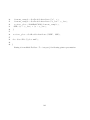
1 v i r t u a l double _evaluate ( I n d i v i d u a l <T>& i n d i v i d u a l )
2 {
3 // a c t i o n #1
4 double o b j e c t i v e _ v a l u e = 0 . 0 ;
5 Chromosome<T>∗ pChrom=i n d i v i d u a l [ 0 ] ;
6
a s s e r t ( pChrom!=NULL ) ;
7 Chromosome<T>& chromosome=∗pChrom ;
8
9
a s s e r t ( ! chromosome . empty ( ) ) ;
10
11 // a c t i o n #2
12
int chromosomeLength=chromosome . s i z e ( ) ;
13
a s s e r t ( chromosomeLength<=this−>getChromosomeLength ( ) ) ;
14
15 //TODO: add c o d e s f o r f i t n e s s c a l c u l a t i o n h e r e
16
for ( int i =0; i <chromosomeLength −1; i ++)
17 {
18
for ( int j=i +1; j <chromosomeLength ; j ++)
19
{
20
int rowDif=abs ( i −j ) ;
21
48
22
int c o l D i f=abs ( chromosome [ i ]−chromosome [ j ] ) ;
23
i f ( rowDif != c o l D i f )
24
{
25
o b j e c t i v e _ v a l u e +=1.0;
26
}
27
}
28 }
29
30 return o b j e c t i v e _ v a l u e ;
31 }
Listing 3.5: Code Listing for modified Problem<T>::_evaluate() method with 8Queens objective function implemented
3.4.4
Compile and Run the Modified Source Codes for 8-Queens
Problem
Now that we have completed the tasks of modifying problem.xml and Problem<T>::_evaluate(),
we can now run the algorithm to solve the 8-Queens Problem. To do this, compile the
source codes using one of the following approaches:
1. If you have VC 6 or VC 2005 installed in your computer, you can just build
the project using adep.dsw (VC 6) or adep.sln (VC 2005). the default build
configuration for adep.dsw and adep.sln is set to Debug mode, so if you are
planning to use the executable for real time running test, you might want to
change the active configuration to Release mode.
2. If you have neither of this tool but has ADEP setup in your computer, simply
double click the compile.bat batch file in the "C1" root_folder (refered to section
3.2) to compile the source codes.
3. If you have ported the modified ADEP generated source codes on an OS other
than Windows, open the compile.bat file which would look something like the
code listing 3.6. The line that starts with "g++ -O3..." in code listing 3.6 is the
compile command, change the directory of the files in this command and copy
49
and run this command in your OS and the source codes will be compiled to the
executable.
1
2
3
4
5
6
7
8
SET PATH=
SET PATH=C: \ Program F i l e s \ADEP\MinGW\ b in
SET LIB=
SET LIB=C: \ Program F i l e s \ADEP\MinGW\ l i b
SET INCLUDE=
SET INCLUDE=C: \ Program F i l e s \ADEP\MinGW\ i n c l u d e
g++ −O3 −Wall −o "C: \ Documents␣ . . .
pause
Listing 3.6: Code Listing for compile.bat
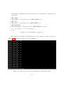
After you have successfully compiled the source codes, run the executable "adep.exe".
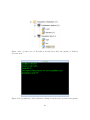
Figure 3.11 illustrate the adep.exe as it is running
Figure 3.11: Screen shot of adep.exe running on 8-Queens Problem
50
Figure 3.11 shows that adep.exe obtain the optimal solution for the 8-Queens Problem in the 71th generation of the Hybrid GA algorithm (for user confused about what
is a generation refer to section 4.2.1 for a short tutorial on Hybrid GA).
3.5
Obtain Solution from ADEP algorithm
In figure 3.11, the solution obtained by the Hybrid GA with integer permutation on
8-Queens is not shown. So how can we obtain the information about the solution as
generated by ADEP algorithm?
For the users who are wondering how to obtain the solution output from the ADEP
algorithm, there are several ways to obtain the solutions from ADEP algorithm that
can be generated at different stage of the algorithm.
3.5.1
Obtain Solution from results.xml
After the running of the adep.exe as described in section 3.4.4, an XML file with the
name "results.xml" is generated in the root_folder "C1". This XML file contains many
useful information about the algorithm. The code listing 3.7 shows the content of the
results.xml as produced by the running of adep.exe
1 <?xml version=" 1 . 0 " ?>
2 <output s i m u l a t i o n _ c o u n t="1">
3
<s i m u l a t i o n i n d e x="1">
4
<g e n e r a t i o n s>
5
<gen g e n e r a t i o n="1"
6
f i t n e s s=" 2 6 . 0 0 0 0 0 0 "
7
time=" 0 . 0 0 0 0 0 0 " />
8
<gen g e n e r a t i o n=" 37 "
9
f i t n e s s=" 2 7 . 0 0 0 0 0 0 "
10
time=" 1 6 . 0 0 0 0 0 0 " />
11
<gen g e n e r a t i o n=" 184 "
12
f i t n e s s=" 2 8 . 0 0 0 0 0 0 "
13
time=" 7 8 . 0 0 0 0 0 0 " />
14
</ g e n e r a t i o n s>
51
15
<s o l u t i o n>
16
<gene i n d e x="0" v a l u e="4" />
17
<gene i n d e x="1" v a l u e="1" />
18
<gene i n d e x="2" v a l u e="3" />
19
<gene i n d e x="3" v a l u e="6" />
20
<gene i n d e x="4" v a l u e="2" />
21
<gene i n d e x="5" v a l u e="7" />
22
<gene i n d e x="6" v a l u e="5" />
23
<gene i n d e x="7" v a l u e="0" />
24
</ s o l u t i o n>
25
<problem d a t e="Thu␣Jun␣ 12 ␣ 11 : 5 8 : 0 1 ␣2008
 ; "
26
chromosome_length="8"
27
best_known_solution=" 2 8 . 0 0 0 0 0 0 "
28
best_known_solution_exist=" t r u e "
29
search_max=" t r u e "
30
/>
31
</ s i m u l a t i o n>
32 </ output>
Listing 3.7: Code Listing for results.xml as produced by the running of adep.exe on
8-Queens Problem
Let us analyze the <simulation> section of the XML code above, the <simulation>
section contains 3 sub sections <generations>, <solution>, <problem>.
1. The <generations> section include information about the fitness change at different generation (for user confused about what is a generation refer to section
4.2.1 for a short tutorial on Hybrid GA), only the generation at which the fitness
change will be recorded in this section, <generations> contains one more more
<gen> elements, each <gen> elements record the generation number, fitness
value at the generation, as well as time from the start running time of adep.exe
in milliseconds
2. The <solution> section include the global best solution found by the algorithm
until the last generation of the algorithm. Therefore this is the solution that the
52
user is looking for the 8-Queens problem. using the information in this section,
the arrangement of 8 queens on the chess board can be easily reconstructed by
treating each <gene> elements in <solution> section as a queen, and its index
and value attributes as the row and column position that the queen occupies.
We can therefore reconstruct the 8-Queens solution as following table 3.3 using
the <solution> section
Queens
row
col
0
0
4
1
1
1
2
2
3
3
3
6
4
4
2
5
5
7
6
6
5
7
7
0
Table 3.3: Arrangement of 8 Queens using the solution provided by results.xml
3. The <problem> section basically record the information that is originally available in the problem.xml in the root_folder "C1", except that it also records the
exact time at which the algorithm is started.
The generation of results.xml file is enabled by default in the algorithm (it can also
be disabled using the ADEP GUI, which we will discuss later). one of the benefits is
that the ADEP generated algorithm is able to record multiple simulations (a simulation
is a run of adep.exe). Therefore if the adep.exe is run twice, then two <simulation>
section will appear in the results.xml file. the code listing 3.8 shows the contents of
results.xml after the adep.exe was run two times.
1 <?xml version=" 1 . 0 " ?>
2 <output s i m u l a t i o n _ c o u n t="2">
3
<s i m u l a t i o n i n d e x="1">
4
<g e n e r a t i o n s>
5
<gen g e n e r a t i o n="1"
6
f i t n e s s=" 2 6 . 0 0 0 0 0 0 "
7
time=" 0 . 0 0 0 0 0 0 " />
8
<gen g e n e r a t i o n=" 37 "
9
f i t n e s s=" 2 7 . 0 0 0 0 0 0 "
10
time=" 1 6 . 0 0 0 0 0 0 " />
11
<gen g e n e r a t i o n=" 184 "
12
f i t n e s s=" 2 8 . 0 0 0 0 0 0 "
53
13
14
15
16
17
18
19
20
21
22
23
24
25
26
27
28
29
30
31
32
33
34
35
36
37
38
39
40
41
42
43
44
45
time=" 7 8 . 0 0 0 0 0 0 " />
</ g e n e r a t i o n s>
<s o l u t i o n>
<gene i n d e x="0" v a l u e="4" />
<gene i n d e x="1" v a l u e="1" />
<gene i n d e x="2" v a l u e="3" />
<gene i n d e x="3" v a l u e="6" />
<gene i n d e x="4" v a l u e="2" />
<gene i n d e x="5" v a l u e="7" />
<gene i n d e x="6" v a l u e="5" />
<gene i n d e x="7" v a l u e="0" />
</ s o l u t i o n>
<problem d a t e="Thu␣Jun␣ 12 ␣ 11 : 5 8 : 0 1 ␣2008
 ; "
chromosome_length="8"
best_known_solution=" 2 8 . 0 0 0 0 0 0 "
best_known_solution_exist=" t r u e "
search_max=" t r u e " />
</ s i m u l a t i o n>
<s i m u l a t i o n i n d e x="2">
<g e n e r a t i o n s>
<gen g e n e r a t i o n="1"
f i t n e s s=" 2 6 . 0 0 0 0 0 0 "
time=" 0 . 0 0 0 0 0 0 " />
<gen g e n e r a t i o n="4"
f i t n e s s=" 2 7 . 0 0 0 0 0 0 "
time=" 0 . 0 0 0 0 0 0 " />
<gen g e n e r a t i o n=" 22 "
f i t n e s s=" 2 8 . 0 0 0 0 0 0 "
time=" 1 5 . 0 0 0 0 0 0 " />
</ g e n e r a t i o n s>
<s o l u t i o n>
<gene i n d e x="0" v a l u e="5" />
<gene i n d e x="1" v a l u e="3" />
54
46
<gene i n d e x="2" v a l u e="0" />
47
<gene i n d e x="3" v a l u e="4" />
48
<gene i n d e x="4" v a l u e="7" />
49
<gene i n d e x="5" v a l u e="1" />
50
<gene i n d e x="6" v a l u e="6" />
51
<gene i n d e x="7" v a l u e="2" />
52
</ s o l u t i o n>
53
<problem d a t e="Thu␣Jun␣ 12 ␣ 12 : 3 3 : 0 8 ␣2008
 ; "
54
chromosome_length="8"
55
best_known_solution=" 2 8 . 0 0 0 0 0 0 "
56
best_known_solution_exist=" t r u e "
57
search_max=" t r u e " />
58
</ s i m u l a t i o n>
59 </ output>
Listing 3.8: Code Listing for results.xml after running of adep.exe two times
3.5.2
Obtain Solution by overriding Problem_Base<T>::interpret()
in the Problem<T> class
For some user who is looking for customized output from ADEP generated algorithm
(for example so that the output can be read and displayed by a GUI), results.xml
might not be suitable. This may be because the user is responsible for the algorithm
design while another developer is working on the GUI, and they have already agreed
on the format of the solution to be passed to the GUI developer, or because the user
is not familiar with XML parsing which is required if the user is going to develop
an GUI to read the results.xml file. In this case, ADEP generated algorithm does
provide a way for the user to create their customize output. This is to override the
Problem_Base<T>::interpret() method in the Problem<T> class. To understand how
this is done, we need to analyze a bit of the ADEP generated algorithm class heirarchy.
The Problem<T> class declared in Problem.h file is a class inherited from the class
Problem_Base<T> class declared in Problem_Base.h (residing in the root_folder\problem
folder). any virtual method declared in Problem_Base<T> can therefore be overriden
55
in Problem<T> class, one of these virtual methods is the Problem_Base<T>::interpret()
method. To override this method, simply copying it into Problem<T> declaration in
the Problem.h file from the Problem_Base.h file. Now with the interpret() method
added into the Problem<T> class, the code listing in the Problem.h file (with comments
omitted and source codes in readInput() and _evaluate() omitted) for the Problem<T>
will look something like the code listing 3.9
1 namespace ADEP
2 {
3 template<c l a s s T>
4
c l a s s Problem : public Problem_Base<T>
5 {
6 public :
7
v i r t u a l bool r e a d I n p u t ( const char∗ f i l e n a m e )
8
{
9
...
10
}
11
12
v i r t u a l double _evaluate ( I n d i v i d u a l <T>& i n d i v i d u a l )
13
{
14
...
15
}
16
17
v i r t u a l void i n t e r p r e t ( I n d i v i d u a l <T>& i n d i v i d u a l )
18
{
19
20
}
21
};
22 }
Listing 3.9: Code Listing for Problem<T> delcaration in Problem.h file with the
virtual method interpret() added
Once the interpret() has been copied into Problem<T> class declaration in the
Problem.h file, Let us try to analyze how this method does and how the user can
56
reimplement the method to obtain the user-desired output solution form.
The interpret() method is automatically called by the ADEP algorithm just before
the program terminates with the global best solution passed to the method(which is
the parameter individual to the interpret() method) to allow the global best solution
to be saved to some form.
There are many ways that the user can reimplement this method, some of the ways
suggested will be
1. the user can directly write the GUI code in Problem<T>::interpret() to display
the solution individual
2. the user can write the information about the individual to another file with his
user-defined format
Just as a simple demo, we are going to output the solution as a table format in a
HTML file output.htm, Code Listing 3.10 list the source codes that we implements in
the interpret() method
1 v i r t u a l void i n t e r p r e t ( I n d i v i d u a l <T>& i n d i v i d u a l )
2 {
3
std : : ofstream o u t f i l e ;
4
o u t f i l e . open ( " output . htm" ) ;
5
6
o u t f i l e << "<html><body>\n" ;
7
8
o u t f i l e << "<t a b l e ␣ b o r d e r=1>\n" ;
9
10 Chromosome<T>& s o l u t i o n =∗( i n d i v i d u a l [ 0 ] ) ;
11
int N=s o l u t i o n . s i z e ( ) ;
12
for ( int i =0; i <N; i ++)
13 {
14
o u t f i l e << "<t r >\n" ;
15
for ( int j =0; j <N; j ++)
16
{
17
i f ( j==s o l u t i o n [ i ] )
57
18
{
19
o u t f i l e << "<td>Q</td>" ;
20
}
21
else
22
{
23
o u t f i l e << "<td>  ;</ td>" ;
24
}
25
}
26
o u t f i l e << "</t r >\n" ;
27 }
28
o u t f i l e << "</t a b l e >\n" ;
29
30
o u t f i l e << "</body></html>\n" ;
31
outfile . close ();
32 }
Listing 3.10: Code Listing for Problem<T>::interpret() method reimplemented
The Code listing 3.10 is a very simple code that print out a table the represents a
chess board with the queens placed in the table (the letter ’Q’) using the arrangement
specified by solution specified in Problem<T>::interpret()
Now recompile ADEP source codes and the runs the compiled adep.exe, after it
is done running, you will find a HTML file output.xml in the root_folder, the figure
belows shows the HTML file when it is open.
3.5.3
Obtain Solutions at Different Generations by Overriding
Problem_Base<T>::record_individual() in Problem<T>
class
For some of the users, outputing the final best solution might not be the only information that he needs, he might also be looking for the trend on how the global best solution
is "evolved" from the first generaton to the last generation. That is, the user might
be looking for the global best solutions generated at each generation of the algorithm.
The overriden Problem<T>::interpret() method simply cannot fullfill this requirement
58
Figure 3.12:
The table printed by output.htm file generated by Problem<T>::interpret()
since it is called only once, at the exit of the program to output the final solution. What
the user should do is to override the Problem_Base<T>::record_individual() method
in the Problem<T> class.
record_individual() is the method called by the ADEP algorithm whenever the
global best solution has changed. Therefore by implementing this method, the user
can save the global best solution whenever that solution has changed.
To override Problem_Base<T>::record_individual() method in the Problem<T>
class, copy and paste the Problem_Base<T>::record_individual() method into the
Problem<T> class declaration in the Problem.h file. 3.11 shows the code listing of the
Problem<T> class declaration (with comments and implementation codes omitted)
after the Problem_Base<T>::record_individual() has been added to Problem.h file
1 namespace ADEP
2 {
3 template<c l a s s T>
4
c l a s s Problem : public Problem_Base<T>
5 {
6 public :
59
7
virtual
8
{
9
...
10
}
11
12
virtual
13
{
14
...
15
}
16
17
virtual
18
{
19
20
}
21
22
virtual
23
24
{
25
26
}
27
};
28 }
bool r e a d I n p u t ( const char∗ f i l e n a m e )
double _evaluate ( I n d i v i d u a l <T>& i n d i v i d u a l )
void i n t e r p r e t ( I n d i v i d u a l <T>& i n d i v i d u a l )
void r e c o r d _ i n d i v i d u a l ( I n d i v i d u a l <T>& i n d i v i d u a l ,
std : : s t r i n g filename )
Listing 3.11: Code Listing for Problem<T> delcaration in Problem.h file with the
virtual method record_individual() added
Let us study the Problem<T>::record_individual() as listed in 3.11, the method is
passed to parameters, individual and filename, the parameter indivuidal the the global
best solution passed to the individual by the ADEP algorithm while the parameter filename is the filename generated by the ADEP algorithm which the user can optionally
use to save the information of global best solution individual in the current algorithm
generation (of course, the user can use his invented file name for the file to which to
save the solution).
Now suppose that we use the filename generated by the ADEP algorithm, and
60
implement the Problem<T>::record_individual() as shown in Code Listing 3.12.
1 v i r t u a l void r e c o r d _ i n d i v i d u a l ( I n d i v i d u a l <T>& i n d i v i d u a l ,
2
std : : s t r i n g filename )
3 {
4
std : : ofstream o u t f i l e ;
5
o u t f i l e . open ( f i l e n a m e . c_str ( ) ) ;
6
7
o u t f i l e << " Current ␣ G e n e r a t i o n : ␣"
8
<< this−>g e t C u r r e n t G e n e r a t i o n ( )
9
<< "\n" ;
10
o u t f i l e << " S o l u t i o n ␣ O b j e c t i v e ␣ Value : ␣"
11
<< i n d i v i d u a l . m _ f i t ne s s [ 0 ]
12
<< "\n" ;
13
14
o u t f i l e << " ////////////////////////////\ n" ;
15
16 Chromosome<T>& s o l u t i o n =∗( i n d i v i d u a l [ 0 ] ) ;
17
int N=s o l u t i o n . s i z e ( ) ;
18
for ( int i =0; i <N; i ++)
19 {
20
o u t f i l e << "Queen␣#" << i
21
<< " : ␣ ( row=" << i
22
<< " , ␣ c o l=" << s o l u t i o n [ i ]
23
<< " ) \ n" ;
24 }
25
o u t f i l e << " ////////////////////////////\ n" ;
26
outfile . close ();
27 }
Listing 3.12: Code Listing for Problem<T>::record_individual() method reimplemented
Now we recompile the source codes and run the adep.exe. After adep.exe is done
running, you should find a new folder "global_solution_records" is placed in the
61
root_folder, in this folder, there are the generation-changed solution files (with filenames "generation##.dat") generated by the algorithm using the format as specified
by Problem<T>::record_individual(), code listing 3.13 shows the content of one of
those file with file name "generation6.dat"
1
2
3
4
5
6
7
8
9
10
11
12
Current G e n e r a t i o n : 6
S o l u t i o n O b j e c t i v e Value : 27
// //////////////////////////
Queen #0: ( row=0, c o l =6)
Queen #1: ( row=1, c o l =0)
Queen #2: ( row=2, c o l =5)
Queen #3: ( row=3, c o l =1)
Queen #4: ( row=4, c o l =4)
Queen #5: ( row=5, c o l =2)
Queen #6: ( row=6, c o l =7)
Queen #7: ( row=7, c o l =3)
// //////////////////////////
Listing 3.13: content of the file generation6.dat in the "global_solution_records" folder
3.5.4
Obtain Solutions for the Entire Population of solutions
for each Generation
There is also ways for the user to print the entire population of solutions at each generations to files by overriding Problem_Base<T>::record_population() in the Problem<T> class declaration. Of course, to print all those data is computationally very
expensive and requires user to have sufficient disk space. normally this option is disabled in the ADEP algorithm (but can be enabled through ADEP GUI). More about
how this can be done will be discussed when it comes to introduce the statistics analysis
capability of ADEP.
62
3.6
Solve a N-Queens Problem
Now that you are quite familiar with the 8-Queens problems and are able to make use
of ADEP-generated source codes to solve the 8-Queens problem, what if you would
like to solve the N-Queen problem, say 100-Queens problem. How should the source
code be modified to do that?
Luckily the source codes require no modification at all, the only change is in the
problem.xml file. Suppose that you are now trying to solve a 100-Queens problem, what you need to do is to open the problem.xml file change the "value" attribute in the "<chromosome_length>" select to 100 and change the "value" in
the "<best_known_solution>" element to 4950 (the total number of not-on-same= 4950, and that’s it.
diagonal constraint violation that can be removed is 100×(100−1)
2
The problem.xml file after modification look likes the code listing 3.14
1 <?xml version=" 1 . 0 " ?>
2 <problem name="100−Queens ␣ Problem ">
3
4 <o v e r v i e w>
5
<chromosome_length v a l u e=" 100 " />
6
<best_known_solution e x i s t e d=" t r u e " v a l u e=" 4950 " />
7
<maximization v a l u e=" t r u e " />
8 </ o v e r v i e w>
9
10 <p a r a m e t e r s>
11 </ p a r a m e t e r s>
12
13 </ problem>
Listing 3.14: Code Listing for problem.xml prepared for 100-Queens Problem
Now rerun the adep.exe without recompiling the source codes and you should
get the solution for the 100-Queens problem (before rerunning adep.exe, delete the
"global_solution_records" folder and the "results.xml").
The source codes for this chapter is included in the ADEP as an example, it can
be found at "[to be fill later]"
63
Chapter 4
Configure ADEP Algorithm
In this chapter, you will learn
1. How to Configure an algorithm to improve its performance
4.1
How to Test Run algorithm on 100-Queens Problem
If you have followed through the Chapter 3 and worked on the examples thouroughly,
you will notice that you would not usually get the global optimal solution for the 100Queens Problem. This implies that the algorithm that is generated by ADEP is not
optimized for an N-Queens Problem by default and therefore you need to configure the
algorithm to optimize it for the N-Queens Problem. There are two ways to do this:
1. expert-mode:
(a) get the documentation to study the algorithm source codes generated by
ADEP,
(b) study the books on Genetic Algorithm,
(c) then study the books on Genetic Algorithm that solve integer-permutation
representation problem,
(d) then begin to tweak the codes generated by ADEP to configure the algorithm.
64
(e) refer now and then if you are not familiar with C++ and its standard
template class implementation
This the approach usually taken by researchers when working with a Genetic
Algorithm library package such as GALib or TOMLab. You will get a lot out
this approach by investing heavily in understand the GA paradigm and implementation while GALib or other GA library saves you times to code many of the
modules. The downside is that the learning curve is steep and you want to solve
your problem urgently
2. ADEP-GUI-mode: Through the GUI of ADEP, you can visually configure the
algorithm and run the test on the algorithm to the point until you are satisfy
with the results produced by the ADEP configured algorithm. To make this an
easier process, you can upload your modified Problem.h file as well as other data
files into the ADEP environment, and have the algorithm automatically combine
the files into the project when compiling and test running. this allow the user to
quickly add in or remove an advanced operator modules or change a parameter
without the need to understand how the coding is done.
In this chapter, we will basically focus on the ADEP-GUI-mode.
As discussed in section 1.3.6, the tranditional way of configuring and then testing
the performance of an algorithm on a problem can be quite tedious when this process
is to be repeated many times, what ADEP-GUI-mode offered is a much faster and
more convenient way of configuring and test running an algorithm. ADEP-GUI-mode
is able to complete this process by using the "project" concept. The concept works
like this:
1. the user first create a TestBench project in the ADEP environment, and
2. then the user upload whatever files that he changed in the generated ADEP
source codes (refer to chapter 3) into the corresponding folders in the created
project directory
3. the user configure the algorithm through ADEP GUI, and
4. then the user click on "Run" command on the Command Panel, and in the
"Run Command" Dialog that appear, select his created project in step 1. ADEP
65
will then combine the configured algorithm with the user-modified files in the
project, and then compile and test run on those hybrid source codes, returning
the performance statistics when it is done.
This section started with the assumption that the user is working on the 100Queens problem, and has modified the problem.xml and the Problem.h file with the
source code compiled and run successfully, but the user was not able to get the best
result that he was looking for. He started by reading the next section 4.1.1.
4.1.1
How to Create Problem TestBench project and upload
files to the project
To create a TestBench project, select menu Run→New Project. the "Create TestBench..." dialog appear which is illustrated in figure 4.1
In the "Create TestBench" dialog in figure 4.1, enter a project name in the "Project
Name" text box, for example, Let us assume "Ex_NQueensProblem" is entered in the
textbox. Click on the "Create New Benchmark" button in the "Benchmark" section,
the "Create Benchmark" dialog appear which is illustrated in figure 4.2. Entering
a name, say, "100QueensBenchmark", into the textbox of the "Create Benchmark"
dialog and press OK. This bring up a "Benchmark Configuration" dialog as shown in
figure 4.3.
The "Benchmark Configuration" dialog in figure 4.3 show very similar layout to
the problem.xml file contents (refer to section 3.4.2 for the problem.xml analysis). The
dialog also consists of "overview" and "parameters" section. This brings up a question,
"What is a benchmark?" which we have not answer up to this point. Remember that
in section 3.4, the ADEP algorithm is designed to be highly flexible, such that the
algorithm is written to work with a problem, but not with a problem instance. To
differentiate a problem and a problem instance. N-Queens Problem will be a problem,
but 100-Queens Problem is a problem instance. what is contained inside the problem.xml file is the problem instance setting (100 Queens Problem setting), whereas
the algorihtm itself can solve the N-Queens problem (remember, to solve 100 Queens
Problem in section 3.6, the source codes does not require to be modified and recompiled at all) and the TestBench project created represent the problem itself (N-Queens
Problem). Now Let us go back to answer the question of "what is a benchmark?":
66
Figure 4.1: The "Create TestBench " Dialog
Figure 4.2: "Create Benchmark" dialog
67
Figure 4.3: The "Benchmark Configuration" Dialog
68
a benchmark is the particular problem setting for a problem instance. When we create the "100QueensBenchmark", we are creating the problem setting for the problem
instance — 100 Queens Problem. The information entered into the "Benchmark Configuration" dialog is highly similar to what is being done to the problem.xml file. figure
4.4 shows the settings entered for the "100QueensBenchmark" configuration dialog.
Figure 4.4: Settings Entered for the "100QueensBenchmark" configuration
When settings are entered in the "100QueensBenchmark" configuration dialog, click
"OK" button. At this point, the user is brought back to the "Create Testbench"
dialog, with the newly created "100QueensBenchmarks.benchmark" appear in the list
box of the "Benchmarks" section. More than one benchmarks can be created for
a particular TestBench project by Clicking the "Create New Benchmark" command
69
Figure 4.5: "Add file" dialog to upload files to the "Ex_NQueensProblem" project
folder
again(Remember earlier in our discussion, the TestBench project represent the problem
while a particular benchmark represent a particular problem instance). a created
Benchmark can be update or delete by selecting the Benchmark in the list box and
pressed the Update or Delete benchmark options also available to the "Benchmarks"
section. To test out these functions, the user can try to add an 500-Queens benchmarks.
After the benchmark is created, the next step is to update the modified source
codes files and other files (changed or added to the generated source codes earlier) to
the project folder. First, Let us upload the Problem.h file that we modified in the
chapter 3. Click "Add File" button in the "Testbench Directory" section, an "Add
File" dialog appear as shown in the figure 4.5
In the "Add File" dialog, click the "Browse", to bring up the "browse for file" dialog,
navigate to the root_folder in which the previously generated source codes were stored
(which is the "C1" folder refered in section 3.1). navigate to the problem folder, and
select the Problem.h file. When this is done, the user is brought back to the "Add
File" dialog with the file path of the selected Problem.h file appearing in the "File to
Upload" text box. Next in the "Directory" drop down list, select "problem" (this allow
ADEP to put the modified Problem.h file uploaded into the corresponding "problem"
folder later during the compiling and testing running stage). Always remember that
whichever folder under the root_folder that you get the modified file from, you should
also set the folder name in the "Directory" drop down list edit box (if it is in the
root_folder, then leave the "Directory" dropdown list edit box empty, if the name of
the folder does not appear in the drop down list, then try it in the edit box). when
this is done, click "OK" on the "Add File" dialog, the user is brought back to the
"Create TestBench" dialog, with "problem\problem.h" appearing in the list box of the
70
"Testbench Directory" section.
In Chapter 3, we modified two files: problem.xml and Problem.h. But we only
uploaded the Problem.h file to the "Ex_NQeensProblem" project folder because the
"100QueensBenchmark" will be translated into the problem.xml file by ADEP during
the later compiling and test running stage. At this point, press the "OK" button on
the "Create TestBench" dialog and this completes the process to create project and
upload files.
One thing to pay attention, although the manual so far only demonstrate Hybrid GA with integer permutation and C++ programming language. ADEP is highly
extensive with other algorithm frameworks, problem representations, and with other
programming language such as Java. The "Ex_NQueensProblem" project is built
only for integer permutation representation and C++ language (the project can work
with other algorithm frameworks with integer permutation though, refered to Section
5.1). The connection between the project and the representation+language setting is
automatically taken care of by ADEP based on the currently select representatin and
language (Remember the title bar of the Diagram Panel that reads "Hybrid GA[Integer
Permutation][cpp], as discussed in section 3.1.1).
To see the created project, select menu Run→TestBench Manager. In the "TestBench Manager" dialog that appear (shown in figure 4.6), select the "Ex_NQueensProblem"
from the "Available TestBenches" list box. When the "Ex_NQueensProblem" is selected in the list box, the "Benchmarks" and the "TestBench Directory" section as
well as the status bar at the bottom of the "TestBench Manager" dialog are automatically updated for the selected project. the status bar reads "The TestBench
<Ex_NQueensProblem> is based on the [cpp] version of an algorithm in Integer
Permutation representation
4.1.2
How to Test Run a ADEP TestBench project
With the "Ex_NQueensProblem" TestBench project properly set up and the modified
files uploaded, it is ready to test run the 100-Queens problem, to do this. Click "Run"
command in the Command Panel of ADEP. In the "Run" dialog that appear (shown
in figure 4.7), select the "Ex_NQueensProblem" from the "Problem" drop down list,
and then select the "100QueensBenchmark" from the "Benchmark" drop down list.
71
Figure 4.6: "TestBench Manager" with the "Ex_NQueenProblem" selected in the list
box
72
Figure 4.7: The "Run" dialog with "Ex_NQueensProblem" and "100QueensBenchmarks" selected
73
Next in the "Run" dialog shown in figure 4.7, select a root_folder to stored the generated source codes by Pressing the "Browse" button. and then select a compiler from
the "Compiler" drop down list. When done, click "OK". ADEP will automatically
perform the following task in order:
1. generate the source codes of the algorithm combined with the files in "Ex_NQueensProblem"
project folder and store them int the root_folder specified in the "Run" dialog
earlier (assume the user selected the root_folder to be "C2")
2. compile the source codes in the root_folder "C2".
3. run the compiled adep.exe file
4. display the statistics in the "Fitness Versus Generation" chart and the "StatisticsInfo" table (as shown in figure 4.8)
Figure 4.8: The "Fitness VS Generation" chart and the "StatisticInfo" table showing
perfomance measure of the generated algorithm after the test running
74
4.1.3
Understand the statistics measure generated by ADEP
during the test run of 100-Queens Problem
Now let us spend some time to understand the statistics produced by test running the
Hybrid GA with integer permutation on the 100-Queens problem. Firstly, we turn
our attention to the "Fitness versus Generation" chart (shown in figure 4.9) which
shows the change of objective value of the global best solution against the generation
number. The Chart can be saved by selecting the menu File→Save from the "Fitness
VS Generation" chart window.
In the "Fitness VS Generation" chart obtained by test running the hybrid algorithm on 100-Queens problem, the curve shows a ascending trend, indicating that the
Hybrid GA is improving the solution quality, the ascending gradient decrease at later
generations which is logical since at the later generations, the solution quality is already quite good and to look for solution with quality better than the currently found
one will be more and more difficult. the maximum objective value obtained is only
4920 which is smaller than the optimal 4950 that we are looking for, suggesting that
the current configuration fail to find the optimal solution.
Next Let us look at the "StatisticInfo table" (as shown in figure 4.10). The recorded
statistics in the table are explained below:
1. Simulation Run at: the time at which the test running is started
2. Number of Simulation: total number simulations or test runs recorded, both "Fitness VS Generations" and "StatisticInfo" can record multiple test runs. Which
will be further explained later.
Ps=N
CP U _time(s)
3. avg CPU time (ms) = s=1 N
where CPU_time(s) is the CPU time
spent for the simulation s and N is the total number of simulations.
4. min CPU time (ms) = min{CP U _time(s)|s ∈ {1, · · · , N }}
Ps=N
total_generation(s)
5. avg Generations= s=1
where total_generation(s) the number of
N
generations spent in simulation s before the algorithm finds the final global best
solution.
6. min Generations=min{total_generation(s)|s ∈ {1, · · · , N }}
75
Figure 4.9: The "Fitness VS Generation" chart obtained by test runing the hybrid GA
on 100-Queens Problem
76
Figure 4.10: "StatisticInfo" table obtained by test running the hybrid algorithm on
100-Queens Problem
Ps=N
best_f itness(s)
7. avg Fitness= s=1 N
where best_fitness(s) is the best fitness/objective
value found for the simulation s and N is the total number of simulations.
(
min{best_f itness(s)|s ∈ {1, · · · , N }} min_search
8. best Fitness=
max{best_f itness(s)|s ∈ {1, · · · , N }} max_search
9. best known solution: the fitness value of the best known solution for the 100Queens Problem, this is the calculated optimal fitness value (entered during the
create of "100QueensProblem" benchmark)
× 100%
10. avg Gap= |avg_F itness−best_known_solution|
best_known_solution
11. min Gap= |min_F itness−best_known_solution|
× 100%
best_known_solution
In case you accidentally close the "Fitness VS Generation" chart and "StatisticInfo"
table, if you are looking for those values recorded in "Fitness VS Generation" chart
and "StatisticInfo" table, you can go to folder "C2" (the root_folder that stores the
77
generated source codes and the compiled adep.exe by ADEP at the time the test run
is conducted) and active the Chart.exe and StatisticInfo.exe to view the results again.
4.1.4
What are the Files and Folders generated during ADEP
Test Run of 100-Queens Problem?
Figure 4.12 shows the list of files and folders in the "C2" folder. Compared the contents
of "C2" with those of "C1" in figure 3.7 of section 3.2, we notice that a few other files
are created, they are
1. Chart.exe, Chart.exe.intermediate.manifest: this is the "Fitness VS Generation
Chart" application
2. StatisticsInfo.exe, results.htm: this is the "StatisticInfo" application
3. cmd.bat: this is the batch file written to invoke Chart.exe and StatisticsInfo.exe
applications at the end of the algorithm test run
4. algorithm_information.xml: this is a generated XML file that describes the algorithm’s representation and programming language used.
5. benchmarks: a folder that contains all the Benchmark files created for the
"Ex_NQueensProblem" project
Among those items, algorithm_information.xml and benchmarks folder are not involved with any processing (they are merely there as information and can be removed
without affecting the algorithm running). The "Fitness VS Generation Chart" application, cmd.bat as well as the "StatisticInfo" application forms the performance
measurement reporting subsystem that is invoke at the time the algorithm is about to
exit.
Now in the folder "C2", double click the adep.exe to run it. An interesting observation will appear: as shown by figure 4.11, just before adep.exe terminates, the "Fitness
VS Generation Chart" and the "StatisticInfo" application are automatically invoked
and both applications showed the statistics information of two simulations instead of
a single simulation! How can this be possible? This is because both "Fitness VS Generation Chart" and "StatisticInfo" are capable of reading and analysing data from the
78
results.xml file described in section 3.5.1. the adep.exe compiled is able to write the
simulation resuls of as many simulations as possible into the results.xml file as long as
it is not deleted before adep.exe is run again.
Figure 4.11: Screen shots at the end of the program execution of adep.exe when run
from folder "C2"
The other question that some of the users might want to ask is what modification is done in the source codes by ADEP such that the compiled adep.exe is able
to invoke the "Fitness VS Generation Chart" and "StatisticInfo" just before adep.exe
terminates? This is actually quite easily done, ADEP simply open the main.cpp file
(located in root_folder\main folder), and add a line system("cmd.bat"); before the return 0; statement in the main() function. So just before adep.exe terminate, it invokes
the cmd.bat batch file, which then invokes "Fitness VS Generation" and "StatisticInfo"
which then reads data from results.xml and display the statistics accordingly.
79
Figure 4.12: The files and folders in the root_folder "C2" generated by the ADEP test
run procedure
4.2
How to Configure an Algorithm to Improve its
Performance
In section 4.1.3, the "Fitness VS Generation" chart obtained by test running the default
Hybrid GA algorithm (this is the same settings as the Hybrid GA algorithm in chapter
3) on 100-Queens Problem showed that the maximum objective value obtained is only
4920. This is smaller than the optimal 4950 that we are looking for, suggesting that
the current configuration of the Hybrid GA algorithm is not optimized to solve the
N-Queens Problem.
In this section, we will show how to configure an algorithm using the ADEP GUI.
The next sections shows how one can configure a Hybrid GA using integer permutation
representation to optimally solve the N-Queens Problem. Section 4.2.2 will illustrate
how to access the code hint of those operators as well). Just to refresh the users’s
memories about the Genetic Algorithm concept, a short introduction of Genetic Algorithm is presented below (Section 4.2.1)followed by a description of the graphical
80
elements in the Functional Block Panel and Node Information Panel (Section 4.2.2)
and a discussion on the default settings for Hybrid GA(Section 4.2.3)
4.2.1
Basic concept of Hybrid Genetic Algorithm
Figure 4.13: Diagram Panel showing the workflow of a Hybrid GA
Figure 4.13 shows the workflow of Hybrid GA in the Diagram Panel. Notice that
the Offspring Mutation functional block has a green color border on its two sides, this
indicates the Offspring Mutation functional block is the currently selcted functional
block. To select a different functional block, click on the functional block in the Diagram Panel and it will be selected. notice that the Functional Block Panel below
the Diagram Panel automatically update the tree control to reflect the operator trees
belonging to the newly selected functional block.
For those users who have already have some basic understanding of Genetic Algorithm using integer permutation representation, they should not have difficulty to
understand this workflow. But to facilitate the understanding of those users who are
new to this field. below is a brief introduction of what each functional blocks in figure
4.13 attempts to do:
81
1. Population Initialization: This generates a population of individual solutions
each of which is a randomly created integer permutation
2. Population Evaluation: This assigns to each of the individual solutions generated
in the Population Initialization a fitness value (fitness value is different from the
objective value in that only the more positive fitness indicate the individual solution is better, this is different from the objective value assigned to an individual
due to objective value having a search direction, there are many ways to convert
an objective value to a fitness value, the simplest way is to invert the sign of the
objective value if the search is minimization, for maximization, simply assign the
objective value as the fitness value)
3. Local Search: This is optional (the default Hybrid GA does not use it). Basically,
this functional block applies local search to the individual solution generated by
Population Initialization.
4. Stopping Condition: this functional block determine the Hybrid GA should terminate and terminate the algorithm when certain termination conditions are
fullfilled. notice it is in a while loop, usually in the terminology of GA, one
single loop of this while loop is considered to be one generation as the population go through reproduction selection, crossover, mutation, local search, survival
selection and so on to generate a new population in one generation.
5. Offspring Producer : this functional blocks select some individuals from the current population into a mating pool (using some selection methods based on the
fitness of the individual solution), and a offspring population of individual solutions is generated from the mating pool by performing crossover between individual solutions in the mating pool Offspring Mutation: this functional blocks try
to mutate some of the individual solutions in the offspring population Offspring
Evaluation: this functional blocks calculate and assign a fitness value for each
individual solution in the offspring population Offspring Local Search: this is
also optional (the default Hybrid GA does not use it). basically it performs local search on certain individual solutions of the offspring population. Population
Updating: this functional block selects individual solutions from both the current
population and the offspring population form the next generation population. it
82
can be seen from figure 4.13, then the next functional block that will be run is
Stopping Condition and hence the generation loop is form.
4.2.2
Understand the symbols used in the Functional Block
Panel and Code Hint available in Node Information Panel
figure 4.14 shows the operator trees displayed in the Functional Block Panel when the
Population Initialization functional block is selected.
Figure 4.14: Operator Tree of the Population Initialization functional block
In figure 4.14, the tree node that has a "(+)" sign next to its caption is the operator
currently selected to be used in the algorithm, the operator tree in figure 4.14 indicates
that the initialization method is Random and the population size is low. What some
observant users will discover now is that in figure 4.14, the operator node with a black
icon is the one that is can is alway selected to be used in the configured algorithm
(this is termed property) whereas the operator node that has an blue icon next to
it is one that can be selected or deselected (this is termed variance). Therefore the
selection of operator node Initialization method (with black icon) is compulsory (In a
GA, one definitely need to one way to initialize the population), but the selection of
the operator node Random under Initialization method (with blue icon) is optional
(In a GA, one do not need to use Random to initialize the population all the time,
83
initialization can be done by using other methods)
To see what each of those operator is about, activate the node that represents
the operator in the Functional Block Panel (by clicking at the node), and the Node
Information Panel to the right of the Functional Block Panel will automatically display
the information of the represented operator. As shown in figure 4.15, the currently
activated operator in the operator tree of Population Initialization is the node Random
under the tree node Initialization Method, the Node Information Panel automatically
display the code hint related to the activated operator node.
Figure 4.15: Random Operator Node being selected in the Functional Block Panel
Let us pay some attention to the code hint displayed in the Node Information Panel
in figure 4.15. The following is a short descriptions of the elements contained in the
code hint in figure 4.14
1. Random is selected : this line tell us that the current operator node Random is
selected to be used in the algorithm
2. Priority Code: used for internal node keeping and the user does not need to
pay particular attention to it. This code can be understood as a code that
is used to indicate the execution order of each operator node in the operator
tree. For example, the operator nodes Initialization Method and Population Size
are at the same node level of the operator tree, but Population Size has Priority
Code "AAA" whereas Initialization Method has Priority Code "AAB", therefore,
Population Size operator will be executed before Initialization method in the algorithm generated by ADEP. (actually, we define the operator precedence rule
using the full Priority Code of the operator node. Since the Population Initialization functional block also has a Priority Code "AAA", the full Priority Code
84
for Population Size is "AAA-AAA" whereas the full Priority Code for Initialization method is "AAA-AAB"). When we compare the Random operator node
under Initialization method and the Low operator node under Population Size,
they are also at the same node level, and both have Priority Code "AAA", but
the full Priority Code of operator node Random is "AAA-AAB-AAA" whereas
that of operator node Low is "AAA-AAA-AAA", therefore operator node Low
is executed by the ADEP generated algorithm than operator node Random
3. Node Id : a unique id assigned to each node and is used for internal node keeping.
The user does need to understasnd its mechanism.
4. Description: This describes the function of the operator or parameter, and how
it can be appropriately used.
Notice there are two command below the Node Information Panel that read "Update" and "Description", the purpose of the "Update" command is to update the
status of the operator node currently activated in the Functional Block Panel and
how to use it is to be discussed in Section 4.2.5. The purpose of the "Description"
command is to display the code hint for the activated operator node in the Functional
Block Panel, but it offers additional information other than those displayed in the Code
Hint of the Node Information Panel. Now with the operator node Random selected in
the Functional Block Panel, click on the "Description" command, A "Operator Node
Description" dialog pop up as shown in figure 4.16
The three tabs in the "Operator Node Description dialog are described below:
1. Operator Description: This is the same as the Description element in the Code
Hint of the Node Information Panel. Due to the size of the Node Information
Panel, longer description may not display fully in the Panel, but the Operator
Description can show the full length description of the operator node
2. Operator Detail : This tab displays the other 3 elements available in the code hint
of the Node Information Panel. Furthermore, it also displays the C++ source
codes file will be transferred from ADEP into the root_folder selected by the
user when activating the "Generate", "Run", or "Learning" commands in the
Command Panel.
85
Figure 4.16: "Operator Node Description" dialog
3. Operator Initialization Code: This is the initialization code that will be used by
ADEP to do the initialization of the activated operator node during the process of algorithm generation. the initialization is editable (if you make change,
the "Update" command will be enabled) but unless the user understand the algorithm design patterns and flow (require the user to be advanced user of the
ADEP system), it is recommended that the user do not attempt to modify the
initialization code
4.2.3
Understand the default configuration of Hybrid GA
Now that we have a basic understanding of the Hybrid GA as well as the graphical
elements in the Functional Block as well as the Node Information, I will explain the
default configuration used by the Hybrid GA in each functional blocks. (The user can
refer to the operator tree of each functional block and the operator information as we
go along this section.
1. Population Initialization:
86
(a) Initialization method is selected as Random indicating the initial population
is a set of individual solution each of which is a random integer permutation
Population Size is selected as low which set [population_size]=20
2. Local Search:
(a) Local Search Method is set to Disabled indicating that no local search will
be applied to the individual solutions in the population
(b) Local Search Frequency is set to Medium ([local_search_frequency=0.5])
but this Local Search Method is Disabled, this parameter is not used
(c) Local Search Sorting is set to None means the population wont be sorted
by fitness
3. Stopping Condition:
(a) Termination
i. Stopping Criteria is set to Generation_Limited indicating the algorithm
will be terminated when certain number of generations is reached Optimal Reached is set to Terminate indicating that if the best known
solution found in the past is available and if the algorithm already find
that solution, then terminate
ii. Stopping Parameters
A. Maximum Duration is set to Low ([max_duration_in_secs]=120),
this parameter is not used as Stopping Criteria is not set to
Time_Limited or Time_Gen_Limited
B. Maximum Generation is set to Low ([max_generations]=2000) indicating the algorithm will terminate after 2000 generations
C. Maximum Stagnation is set to Low ([max_stagnation_count]=300),
this parameter is not used as Stopping Criteria is not set to Stagnation_Gen_Limited
(b) Update Global Solution
i. Record Candidate Solutions is set to Disabled indicating the
Problem<T>::record_population() (referred to Section 3.5.4) will not
be called
87
ii. Record Solution in XML is set to Enabled indicating that the results.xml
will be generated (referred to Section 3.5.1)
4. Offspring Producer
(a) Fitness Scaling is set to No Scaling indicating that the fitness of the individual solutions will not be scaled before the Selection of individuals into
mating pool is started
(b) Parent Selection
i. Parent selection method is set to Random indicating the individual solutions are randomly picked from the current population into the mating
pool
ii. Mating Pool Size is set to Low ([selected_parent_count]=2) indicating
that only 2 individual solutions are selected from the current population
into the mating pool
(c) Cross Over
i. Cross Over Method is set to Two Point
ii. Cross Over Rate is set to High ([crossover_rate]=1.0) indicating that
Two Point Crossover will be applied to all pairs of individual solutions
in the mating pool to generate children for the offspring population. (if
it is less than 1, then some pairs of individual solution in the mating
will be copied directly into the offspring population
5. Offspring Mutation
(a) Mutation Method is set to k Swap
(b) Mutation Rate is set to High ([mutation_rate]=0.01) indicating that each
individual solution in the offspring population will have 1% chance of mutation
6. Offspring Local Search:
(a) Offspring Local Search Method is set to Disabled indicating that no local
search will be applied to the individual solutions in the offspring population
88
(b) Offspring
Local
Search
Frequency
is
set
to
Medium
([local_search_frequency=0.5]) but this Offspring Local Search Method is
Disabled, this parameter is not used
(c) Offspring Local Search Sorting is set to None means the offspring population
wont be sorted by fitness
7. Population Updating
(a) Survival is set to Worst Replacement indicating only the least fit individual
in the current population will be replaced by the best individual solution in
the offspring population (and this only happen if the least fit individual in
the current population is not better than the best individual in the offspring
population). This strategy is known as the "Steady State" Replacement
(b) Divergence is set to Disabled indicating that the population will not be
re-boiled when convergence occurs
For the users who are familiar with the concept of Hybrid GA or Memetic Algorithm, the default Hybrid GA is not actually a Hybrid GA but a canonical Genetic
algorithm with steady-steady population replacement since local search is not used to
improve the indivdiual solution in the populations.
4.2.4
Use ADEP "Statistics" panel to view the currently selected operators and parameter settings
ADEP provides extra feature for the users to view all the current configuration, select
from ADEP menu Statistics→Parameters, and the "Statistics" dialog will appear as
shown in figure 4.17 which shows the currently configured settings of the algorithm
4.2.5
How to Configure ADEP algorithm using the GUI
Now we have understand the default configuration of the Hybrid GA in ADEP and we
wish to make the following change from the default configuration:
1. Population Initialization
89
Figure 4.17: "Statistics" dialog showing the currently configure algorithm
(a) Set Population Size to Medium and set the [population_size] parameter in
Medium to 60
2. Stopping Condition
(a) Termination
i. Stopping Parameters
A. Set Maximum Generations to Medium
3. Offspring Producer
(a) Parent Selection
i. Set Mating Pool Size to High and set the parameter [selected_parent_count]
in High to 60 (therefore the offspring population size will also be 60 since
two parents produce two children)
ii. Set Parent Selection Method to Roullet Wheel
90
4. Offspring Mutation
(a) Set the parameter [mutation_range] in k Swap under Mutation Method to
0.005
(b) Set the parameter [mutation_rate] in High under Mutation Rate to 0.2
5. Population Updating
(a) Set Survival to (mu+lambda) Selection, this operator will combine the 60
individual solution in the current population with the 60 individual in the
offspring population and pick the 60 most fit individuals from the 120 individual as the population into the next generation
To make changes suggested above, we need to update the operator tree at each of
those functional blocks. Let us start with the Population Initialization, Select the Population Initialization functional block in the Diagram Panel, in the operator tree of the
Functional Block Panel, Select Population Initialization←Population Size←Medium
branch by double clicking the Medium operator node (or activate Medium operator
node and click "Update" command under the Node Information Panel). A "Operator
Node Configuration" dialog will pop up as shown in figure 4.18
At the bottom of the "Operator Node Configuration" dialog as shown in figure
4.18 is a radio button that reads "Select This Node" and is unselected, proceed to
select the radio button (this will select the operator node). Next select the line the
reads "[pop..." in the list box, this will enable the parameter [population_size] to be
displayed in the text fields below the list box as shown in figure 4.19
In the "Value" text fields of the dialog shown in figure 4.19, change the value of the
[population_size] from 50 to 60, and click the "Close" button on the "Operator Node
Configuration" dialog.
figure 4.20 shows that change in the operator tree in the Functional Panel after the
operator node update above, and figure 4.21 shows the change in the [population_size]
in the Node Information Panel.
One thing to take notice is that although we did not deselect Low under Population,
when Medium under Population is selected, Low is automatically deselected, ADEP
makes sure that conflicting settings wont be selected at the same time.
91
Figure 4.18: "Operator Node Configuration" dialog for the Medium operator node
under Population Size operator node
Figure 4.19: "Operator Node Configuration" dialog with the parameter [population_size] selected in the list box
92
Figure 4.20: operator tree of Population Initialization after the update of Medium
operator node
Figure 4.21: [population_size] is shown to change to 60 after the operator node update
93
The Stopping Condition←Termination←Stopping Parameters←Maximum Generations←Medium can be selected by double clicking the operator node and select the
radio button "Select This Node" in the "Operator Configuration" dialog that pops up
The Offspring Producer ←Parent Selection←Mating Pool Size can be manipulated
in the similar way as the above. To select Offspring Producer ←Parent Selection←Parent
Selection Method ←Roulette Wheel, double clicking the operator node, and select the
radio button in the "Operator Node Configuration" dialog that pop up and then close
the dialog.
The rest of the configuration is left as an exercise to the users as they take basically
the same steps as the above processes.
When the configuration is done, test run the 100-Queens Problem again (refer to
Section 4.1 on How to do the test run).
Figure 4.22: "Fitness VS Generation" Chart display for the 100-Queens test run after
the configuration
figure 4.22 shows that the solution quality found by the algorithm improves from
4922 to 4947.
figure 4.23 shows that the solution with fitness 4947 is obtained after 4.500 seconds
is longer than the default configuration since the algorithm is now allowed run 6000
94
Figure 4.23: "Statistics Info" table display for the 100 Queens test run after the configuration
generations (instead of the default 2000) and the population size also increases.
Although the improvement of fitness has been observed after the configuration, this
is still not the optimal solution. let us now select the operator node Offspring Local
Search←Local Search Method ←Two Genes Swap Step from the currently configured
algorithm, and to the test run again.
The "Fitness VS Generation" chart in figure 4.24 shows that this time the algorithm
finds the global optimal solution with fitness 4950 in the 113-th generation
The "StatisticsInfo" table in figure 4.25 shows that it took 40.8 seconds for the
newly configured algorithm to find the optimal solution.
Now restart ADEP, and from the default configuration, make the following changes:
1. select Offspring Local Search←Local Search Method ←Two Genes Swap DFL
2. select Offspring Local Search←Local Search Frequency←High
And test run the 100-Queens Problem again
figure 4.26 shows that the optimal solution with fitness 4950 is obtained in 11th
generation.
95
Figure 4.24: "Fitness VS Generation" chart for test running 100-Queens after the Two
Genes Swap Step is selected
Figure 4.25: "Statistics Info" table for test running 100-Queens Problem after Two
Genes Swap Step is selected
96
Figure 4.26: "Fitness VS Generation" Chart for test running 100-Queens Problem
after selecting Two Genes Swap DFL
Figure 4.27: "Statistics Info" table for test running the 100-Queens Problem after Two
Genes Swap DFL is selected
97
figure 4.27 shows that the optiaml solution is obtained in 1.5 seconds which is way
faster than the previous configuration that obtain the optimal solution.
The above shows 3 configurations, each of which improves the solution quality of
the final solution obtained by the configured algorithm, with the last configuration
obtained the best results in terms of solution quality and times spent. But this is by
no means all the configurations that are possible to be tried out and there might be
even better configuration than the last configuration shown above.
4.2.6
How to Save a Configuration
What the user will notice is that whenever the user make changes to the current
configuration, the configuration setting change and the previous configuration cannot
be kept. Moreover, when the user want to get back the default configuration, he
has to close the ADEP application and then reopen it. This is quite inconvenient,
especially when the user has already found an good configuration but want to try
some other configurations. ADEP solve this problem by providing feature to save the
user configured settings into *.adep file which can be loaded back into ADEP by double
clicking the file or select ADEP menu File→Open.
To save the current algorithm configuration settings to the *.adep file, select ADEP
menu File→Save or File→Save As.
The intereting feature is that adep automatically save configuration settings in
all the algorithm framework available in ADEP including the different representation
as well as language, so if you configure an algorithm in integer permutation representation and another algorithm in binary representation (selection of representation
will be discussed later chapters), both of these two algorithm settings will be saved
automatically.
the *.adep file is written in XML format and so is human reader, to open the file in
applications other than ADEP to view its content, right click the file and select "Open
With" popup menu. figure 4.28 shows the myConfig.adep file open in notepad.
98
Figure 4.28: myConfig.adep file opened in notepad
99
Chapter 5
Working With Various Algorithms
So far we have been working with the Hybrid GA with integer permutation representation on the N-Queens Problem. But ADEP is not merely application that generate
Hybrid GA using integer permutation. Currently ADEP supports Hybrid GA using
integer permutation representation, binary string representation, and floating point
value representation. Apart from the Hybrid GA, ADEP also support code generations of other popular meta-heuristic algorithms that include Simulated Annealing,
Tabu Search, Ant Colony Optimization, Multiple Random Restart Adaptive Search.
This chapter you will learn:
1. How to switch between different algorithm, representation, and language within
ADEP?
2. Brief description of Hybrid GA with different representations
3. Brief description of other meta-heuristic algorithms
5.1
How to Switch Between Different Algorithms, Representations, and Languages within ADEP?
5.1.1
Select Simulated Annealing algorithm
Start the ADEP application, and click the command that reads "Hybrid GA" in the
Algorithm Panel (which is below the Command Panel in the ADEP GUI). The "Al100
Figure 5.1: "Algorithm Selection" dialog pop up after click the button in the Algorithm
Panel
gorithm Selection" dialog appear as shown in figure 5.1
In the "Algorithm Selection" dialog as shown in figure 5.1, The "Language" drop
down list display the currently use programming language is cpp (C++). The "Representation" drop down list display the currently used representation for problem solution. Below These two drop down lists are the algorithm drop down list that display
"Hybrid GA" which is the currently used algorithm. At the bottom of the "Algorithm
Selection" dialog is a information panel that displays some brief description of the
current algorithm.
Now in "Algorithm Selection" dialog, with the "Language" and "Representation"
unchanged, select "Simulated Annealing" from the algorithm drop down list. Notice
that the information panel at the bottom automatically updates and display a brief
paragraph describing Simulated Annealing algorithm. this is shown in figure 5.2
With "Simulated Annealing" selected in the algorithm drop down list, click OK.
The user is brought back to the ADEP GUI, but this time, The Diagram Panel shows
the work flow of the Simulated Annealing algorithm as shown in figure 5.3
With the newly selected algorithm framework displayed in the Diagram Panel, the
techniques discussed in previous sections are all applied.
101
Figure 5.2: "Algorithm Selection" dialog with Simulated Annealing selection
Figure 5.3: Diagram Panel showing Simulated Annealing algorithm workflow after the
change in "Algorithm Selection" dialog
102
5.1.2
Generate and Modify Simulated Annealing Algorithm
Source Codes to solve N-Queens Problem
this part is exactly the same as that for Hybrid GA as discussed in chapter 3. Just follow
the same steps to modify problem.xml and Problem.h file in the root_folder\problem
folder
5.1.3
Test Run Simulated Annealing algorithm on the 100Queens Problem
Remember that in Section 4.1 at which we create a TestBench project
"Ex_NQueensProblem" with a benchmark "100QueensBenchmark", the project is created in an environment in which Hybrid GA, integer permutation representation, and
C++ languages are 3 selected settings. ADEP’s algorithm framework design allow
this project to be seamlessly incorporated into other algorithms as long as integer
permutation and C++ languages are the other selected settings. In the environment that we have just configured, Simulated Annealing, integer permutation and
C++ language are the selected settings. therefore, we can use the previously created "Ex_NQueensProblem" project to test run the Simulated Annealing algorithm
without any modification required. To test run the Simulated Annealing algorithm
on the 100-Queens Problem, following the instructions in Section 4.1. That is, click
on the "Run" Command in the Command Panel, in the "Run" dialog appear select "Ex_NQueensProblem" from the "Problem" drop down list and "100QueensBenchmark.benchmark" from the "Benchmark" drop down list. and then selected a
root_folder to store the generated source codes as well as a compiler from the "Compiler" drop down list. Finally, press OK. The generated Simulated Annealing (with
the "Ex_NQueensProblem" project incorporated) should be compiled and run successfully. figure 5.4 shows that "Fitness VS generation" chart and the "StatisticInfo"
table displayed when the Simulated Annealing test run on 100-Queens Problem was
completed.
103
Figure 5.4: "Fitness VS Generation" and "StatisticInfo" Application invoked at the
exit of Simulated Annealing algorithn on 100-Queens Problem
104
5.1.4
Configure Simulated Annealing Algorithm through ADEP
GUI
This part is the same as that for Hybrid GA in chapter 4, the user, with some experience
in Simulated Annealing, and under the guide of Code Hint as well as the Code Library
Help, should have no problem understand the various operators and how they can be
changed for configuration.
5.2
Understand Hybrid GA under different representations
different optimization problem usually require different solution representation in order
to be solved naturally and optimally. Among the most common representations are
binary string, integer permutation, and floating point string. To Select Hybrid GA
with a different representation, click the button in the Algorithm Panel of ADEP GUI.
and select the representation from the "Representation" drop down list (floating point
string option is labeled "Continuous" in the drop down list).
If you have read through the previous chapters on the example of N-Queens Problem, you should be quite familiar with the integer permutation by now. For those
user who are not familiar with binary and floating point strings representations, the
following some some examples of the 3 representations.
0
5
3
7
2
4
1
8
9
Table 5.1: An integer permutation of length 10
1.
0
1
1
0
1
1
1
0
1
Table 5.2: A Binary string of length 10
2.
3.
105
0.345
7.23
8.8888
Table 5.3: A Floating point string of length 3
Binary string is most commonly used representation and prevalent in the theory of
Genetic Algorithm. Altough almost all the problems can be represented using binary
strings, some times it is more natural and efficient to represent a solution as an integer permutation or floating point string. For example, a TSP represented by integer
permutation help remove a number of constraints on the problem and make the search
much faster than binary string represented TSP. Similarly, for problem such as finding
optimal parameters for curve fitting (also known as linear and non-linear regression
problem), floating point string may be a better choice for representation.
Although any of Hybrid GAs using different representations share similar work
flow and framework, the operators they use, such as crossover, mutation, local search
and so on, are vastly different. figure 5.5 show a comparison of the operator trees in
the Offspring Muation functional block for Hybrid GA with integer permutation and
binary string respectively.
Figure 5.5: Comparison between the Offspring Mutation operator trees for Hybrid
GAs with Integer Permutation and Binary string representations respectively
106
In the following chapter, some problems which are solved by Hybrid GA with binary
and floating point strings as well as integer permutations will be discussed. For now it is
sufficent to know that all the algorithm in ADEP share the same algorithm framework
design as well as data structures, and the users would be happy to know that whatever
they have learned in the previous chapters applied to any algorithms, with any
respresentation, written in any language.
5.3
Brief Descriptions of the Meta-Heuristic algorithms
available in ADEP
5.3.1
Simulated Annealing
Figure 5.6. Let me explain what happened at each functional block using integer
permutation as the solution representation.
Figure 5.6: Work flow of Simulated Annealing algorithm in the Diagram Panel
1. Initialization: a population of individual solutions are generated such that each
solution is a randomly generated integer permutation. This functional block also
initialize the annealing temperature Ts for each solution s
2. Population Evaluation: this functional block calculate and assign an objective
value for each individual solution in the population
107
3. Stopping Condition: this functional block determine the Simulated Annealing algorithm should terminate and terminate the algorithm when certain termination
conditions are fullfilled. notice it is in a while loop which we have called a generation (refer to Section 4.2.1). In this functional block , the global best solution
sbest is also updated if its fitness is found to be less than one of the individual
solution in the population.
4. Anneal : the main mechanism of Simulated Annealing known as Metropolis process is executed in this functional block. the Metropolis process runs on each
individual solution in the population. We illustrate the Metropolis process on an
individual solution s as follows
for i = 0 to M-1
s0 = neighboring_solution(s)
∆f = f itness(s) − f itness(s0 )
if ∆f < 0 then
if f itness(s0 ) > f itness(sbest ) then
sbest = s0
end if
s = s0
else
r = rand(0, 1)
) then
if r ≤ exp(− ∆f
Ts
0
s=s
end if
end if
end for
where sbest is the global best solution of the algorithm, s0 is the neighboring
solution generated from the current solution s by mutation. M is call the MonteCarlo steps. Ts is the annealing temperature of current solution s The default
setting for the Disturb Mechanism that mutate the current solution s to obtain
the neighboring solution s0 is Two Genes Swap in which two genes are randomly
selected from the integer permutation chromosome of s and swapped.
108
5. Lower Temperature: this functional block applied the cool schedule for the annealing tempature Ts of each individual in the population. The default setting
for the Lower Temperature is Multiplication which is the a cool schedule that set
the new annealing temperature Ts for a solution s by
Ts = Ts × α
where α is a value close to 1 but is smaller than 1.
5.3.2
Tabu Search
Figure 5.7: Diagram Panel showing work flow of Tabu Search algorithm
figure 5.7 shows the work flow of Tabu Search Algorithm in the Diagram Panel when
"Tabu Search" with "Integer Permutation" representation and "C++" language are
selected in the "Algorithm Configuration" Dialog. We will explain what has happened
in each of the functional blocks
1. Initialization: In this functional block , a population of individual solutions are
randomly generated integer permutation. in additional, for each of those solution
a tabu list is created.
2. Population Evaluation: In this functional block, an objective value is calculated
and assigned to each individual solution in the population
109
3. Stopping Condition: this functional block determine the Simulated Annealing algorithm should terminate and terminate the algorithm when certain termination
conditions are fullfilled. notice it is in a while loop which we have called a generation (refer to Section 4.2.1). In this functional block , the global best solution
sbest is also updated if its fitness is found to be less than one of the individual
solution in the population.
4. Navigate Neigborhood : in this functional block, for each solution s in the population, a disturbance mechanism generates a temptative move that can transit the
current solution s to another solution s0 in the neighborhood of s. If this temptative move is not tabued (a move is defined as tabued if its tabu value in the tabu
list is higher than a threshold value) or the move pass some aspiration criteria
(for example, the solution s0 reached from the current solution s by the move
has a fitness value higher than the current solution s), in either case, the fitness
different ∆f = f (s0 ) − f (s) is recorded. After a neighborhood of s of certained
defined size has been searched, the temptative move movebest that produce the
highest ∆f (movei ) is selected to be the next move and is recorded for s.
5. Perform Move: in this functional block, for each solution s in the population, if
the movebest is available for s, the move is performed to transit s to its neighboring
solution s0 , and the tabu value of movei in the tabu list is increased by an amount
known as tabu tenure and the move is tabued (usually moves that move cannot
be selected at least in the next tabu-tenure steps)
6. Update Tabu List: in this functional block, the tabu list is updated, usually
meaning all the moves recorded in the tabu list have the tabu values decreased
by 1, so that after tabu-tenure generations, the movei that is tabued in the
current generation can become non-tabu move again.
7. Update Global Solution: in this functional block, the best individual solution in
the current population is selected, and if its fitness value is higher than the global
best solution sbest , sbest is updated to that best individual solution in the current
population.
110
5.3.3
Ant Colony Optimization
The ant colony optimization algorithm (ACO), introduced by Marco Dorigo in 1992
in his PhD thesis, is a probabilistic technique for solving computational problems
which can be reduced to finding good paths through graphs. They are inspired by the
behaviour of ants in finding paths from the colony to food.
In ACO, the solution of a problem is usually the tour traversed by an ant. The tour
consists of a sequence of states that the ant visit as that ant wonder on a state map
guided by the heuristic cost between two states as well as the pheromone deposited
on the arc between two states. For integer permutation, a state is represented by an
integer and a tour is therefore an integer permutation since each state cannot be visited
more than once usually.
Figure 5.8: workflow of the Ant Colony Optimization algorithm displayed in the Diagram Panel
Figure 5.8 shows the work flow of the Ant Colony Optimization algorithm in the
Diagram Panel which is selected by selecting the algorithm in the drop down list in the
"Algorithm Selection" dialog. The default configuration of ACO algorithm in ADEP
is the Ant Colony System. We will discuss the mechanism involved in each functional
block as shown in the work flow of default configured ACO algorithm.
1. Map Initialization: in this functional block, the state map is created an an initiail
pheromone τ0 is deposited on each arc between any two states that an ant might
traversed.
111
2. Ant Reset: This is the start of a ACO generation, a population of ants are
generated, and each ant is randomly placed at a state initially .
3. Tour Construction: In this functional block, each ant in the population is set
to wonder on the state map to create an ant tour. the process of ant tour
construction is described in the following pseudo code:
for i=0 to N − 1
for each anti in ant_population
Do: state_transition(anti )
end for
end for
where N is the total number of states that an ant can possibly reached. In the
state_transition() method, anti checks if it can move from its current state r to
any other unvisited states. If no, then anti stops and its tour is considered to
be completed. If yes, anti select the next state s to move according to probability p(r, s). The state transition probability p(r, s) is determined by using the
so-called pseudo-random proportional state transition rule. In pseudo-random
proportional state transition rule, a random number p between 0 and 1 is generated and compared with Q0 (a constant between 0 and 1 known as Exploitation
Bias).
if p ≤ Q0 then
(
p(r, s) =
1 s = argmaxu∈Ji (r) {[τ (r, u)]α · [η(r, u)]β
0 otherwise
else
(
p(r, s) =
P
[τ (r,s)]α ·[η(r,s)]β
α ·[η(r,u)]β
u∈Ji (r) [τ (r,u)]
0
s ∈ Ji (r)
(5.1)
(5.2)
otherwise
end if
In equation 5.1 and 5.2, τ (r, u) is the pheromone deposited on the arc from
current state r to neighboring state u. η(r, u) is the heuristic cost from current
112
state r to u. Ji (r) is the set of neighboring states from r that have not been
visited by anti . α is pheromone weight. β is heustic cost weight.
Equation 5.1 perform exploitation search in that the next state selected is a
neighboring state s ∈ Ji (r) such that the product [τ (r, s)]α · [η(r, s)]β ≥ τ (r, u)]α ·
[η(r, u)]β for all u ∈ Ji (r)
Equation 5.2 perform exploration search and is known as random proportional
rule.
when anti finds the next state to move s, it transits from r to s, and perform a
local pheromone update by
τ (r, s) = (1 − ρ) × τ (r, s) + ρ × ∆τ (r, s)
(5.3)
Equation 5.3 is applied to the currently traversed arc (r, s) so as to reduce the attractiveness of (r, s) to other ants (τ (r, s) is reduced), this encourage exploration.
ρ is between 0 and 1.
4. Calculate cost: in this functional block, an objective value is calculated and
assigned to each ant tour generated in Tour Construction
5. Local Search: Local search technique is applied to each ant tour (optional and is
not selected by default configuration)
6. Select Best Ant Tour : the ant tour that has the highest fitness is selected from
all the ant tours generated by the current ant population. if the fitness of the
best ant tour is greater than the fitness of the global best ant tour obtained so
far, the global best ant tour is updated to the best ant tour generated by the
current ant population.
7. Termination Condition: this functional block determine whether the algorithm
should terminate and terminate the algorithm when certain condition have been
fullfilled
8. Pheromone Update: The pheromone on each arc between any two states in the
113
state map is updated by using the global best ant pheromone update rule
τ (r, s) = (1 − α0 ) × τ (r, s) + α0 × ∆τ (r, s)
where
(
∆τ (r, s) =
1
Lgb
(r, s) ∈ tourgb
0
otherwise
(5.4)
(5.5)
In Equation 5.5, Lgb is the number of states visited by the global best tour tourgb .
5.3.4
Simple Random Search
Figure 5.9: work flow of Simple Random Search displayed in the Diagram Panel
Figure 5.9 shows a Simple Random Search algorithm. this algorithm can be easily
configure as a multple individual local search algorithm or a multiple random generated
algorithm or the combination of both. we will briefly go through its functional blocks.
1. Randomize: this functional block generate a population of randomly generated
individual solutions if the population has not been created or mutate the individual solution if the population exists already (optional)
2. Population Evaluation: this functional block assigns a calculated objective value
to each individual solution in the population.
114
3. Local Search: Local search to be applied to the individual solution in the population (optional)
4. Stopping Condition: control the termination of the algorithm.
by using different configuration, the Simple Random Search algorithm can be
changed to a single solution local search, or a multiple individual local search, or a
multiple solution mutation-improving algorithm and so on.
115
Chapter 6
ADEP Example: Quadratic
Assignment Problem
The quadratic assignment problem (QAP) is one of fundamental combinatorial optimization problems in the branch of optimization or operations research in mathematics,
from the category of the facilities location problems.
The problem models the following real-life problem:
There are a set of n facilities and a set of n locations. For each pair
of locations, a distance is specified and for each pair of facilities a weight
or flow is specified (e.g., the amount of supplies transported between the
two facilities). The problem is to assign all facilities to different locations
with the goal of minimizing the sum of the distances multiplied by the
corresponding flows.
The problem statement resembles that of the assignment problem, only the cost
function is expressed in terms of quadratic inequalities, hence the name.
116
Chapter 7
ADEP Example: Traveling Salesman
Problem
117
Chapter 8
ADEP Example: Regression Analysis
In this chapter, you will learn
1. What is Regression Analysis?
2. How to solve a regression analysis problem?
3. How to represent the parameters solution as binary string in binary GA
4. How to represent the parameters solution as floating point string in Continuous
GA
5. How to define objective function for regression analysis
6. How to use ADEP to generate and modify codes to solve regression problem?
8.1
8.1.1
What is Regression Analysis?
Regression Explained
Regression analysis is a technique used for the modeling and analysis of numerical data
consisting of values of a dependent variable (response variable) and of one or more independent variables (explanatory variables). The dependent variable in the regression
equation is modeled as a function of the independent variables, corresponding parameters ("constants"), and an error term. The error term is treated as a random variable.
118
It represents unexplained variation in the dependent variable. The parameters are estimated so as to give a "best fit" of the data. Most commonly the best fit is evaluated
by using the least squares method, but other criteria have also been used.
Regression can be used for prediction (including forecasting of time-series data),
inference, hypothesis testing, and modeling of causal relationships.
8.1.2
Linear Regression Explained
In linear regression, the model specification is that the dependent variable, y is a linear
combination of the parameters (but need not be linear in the independent variables).
For example, in simple linear regression for modeling N data points there is one independent variable x, and two parameters β0 and β1 :
y = β0 + β1 x (straight line)
as shown in figure 8.1
Figure 8.1: a Simple Linear Regression Model
119
In multiple linear regression, there are several independent variables or functions
of independent variables, an example can be
y = β0 + β1 x1 + β2 x21 + β3 cos(x2 ) + β4 tan(x1 )
This is still linear regression as although the expression on the right hand side is
non-linear in the independent variable x1 and x2 . it is still linear in parameters β0 , β1 ,
β2 , β3 , and β4 .
8.2
A Simple Linear Regression Example
Given below is the table of data points sampled from a system:
x
10
20
31
40
50
100
y
2.569
2.319
2.058
1.911
1.598
0.584
Table 8.1: Data Sample from a System
Assume the system can be modelled by yi = β0 + β1 xi + i , where i is an error term
and the subscript i indexes a particular observation. our objective is to find values βˆ0
and βˆ1 in a linear regression yi = βˆ0 + βˆ1 xi such that the linear regression best fit the
data points in table 8.1.
8.2.1
Least Squares Method
ei = yi − (βˆ0 + βˆ1 xi ) is called the residual. To find βˆ0 and βˆ1 , the least squares method
can be used. In this method, we are to find the values of βˆ0 and βˆ1 such that
E=
i=N
X−1
i=0
e2i =
i=N
X−1
[yi − (βˆ0 + βˆ1 xi )]2
i=0
is minimized.N is the number of data points sampled.
120
(8.1)
8.2.2
Weighted Least Squares Method
One of the common assumptions underlying linear and nonlinear least squares regression, is that each data point provides equally precise information about the deterministic part of the total process variation. In other words, the standard deviation of the
error term is constant over all values of the predictor or explanatory variables. This
assumption, however, clearly does not hold, even approximately, in every modeling
application. In situations like this, when it may not be reasonable to assume that
every observation should be treated equally, weighted least squares can often be used
to maximize the efficiency of parameter estimation. This is done by attempting to
give each data point its proper amount of influence over the parameter estimates. A
procedure that treats all of the data equally would give less precisely measured points
more influence than they should have and would give highly precise points too little
influence. In weighted least squares method, the objective is to find the values of βˆ0
and βˆ1 such that
E=
i=N
X−1
i=0
wi e2i
=
i=N
X−1
wi [yi − (βˆ0 + βˆ1 xi )]2
(8.2)
i=0
is minimized wi in equation 8.2 is used to estimate the values of the unknown parameters are inversely proportional to the variances at each combination of dependent
variable y
1
(8.3)
wi ∝ 2
σi
There are a number of ways to estimate wi in equation 8.2, interested readers can
refer to literatures on feasible Weighted Least Squares, or iterated 2-steps Weighted
Least Squares methods.
8.3
Simple Linear Regression using ADEP Generated
algorithm with Binary Solution Representation
In this section, we will show how solve simple linear regression using ADEP generated
algorithm with binary solution representation, the algorithm that we would be using
is the Hybrid GA, with code generated in C++.
121
8.3.1
Represent Simple Least Squares Solution using Binary
String
The solution of the simple least squares regression is the values βˆ0 and βˆ1 in y = β0 +β1 x
that best fit the samples (x, y) in table 8.1.
We need to find a decoding method to translate a binary string into the floating
point values of βˆ0 and βˆ1 . There are several ways to do this. But first of all we need
to know roughly the upper bound and lower bound of both parameters, let βˆ0 max and
βˆ0 min be the upper and lower bounds for βˆ0 , and βˆ1 max and βˆ1 min be the upper and
lower bounds for βˆ1 .
assume that we have a binary string chromosome of length 2l, we divide the chromosome into two section of equal length. Each section will then represent the value
of β̂i , i = 0, 1. For each of those chromosome sections, the maximum value will be a
binary string of l 1’s, this can be convert to a maximum decimal value zmax = 2l − 1,
the minimum binary value will be a binary string of l 0’s, this can be verted to a minimum decimal value of zmin = 0, we must then convert the decimal value z obtained
by binary-to-decimal conversion, to a value β̂i which will be in the range of value to
between βˆ0 .
Let us try an example, suppose that the binary string chromosome is
1
1
0
1
1
0
1
0
Table 8.2: binary string chromosome
we divide the binary string 8.2 into two chromosome section of length 4 as shown
below
1
1
0
1
Table 8.3: chromosome section for βˆ0
1
0
1
0
ˆ 1
Table 8.4: chromosome section for beta
122
Binary Decoding Method 1
In this method, we translate the binary string in 8.3 to decimal value z(βˆ0 ) = 1 ·
23 + 1 · 22 + 0 · 21 + 1 = 13, and the binary string in 8.4 to decimal value z(βˆ1 ) =
1 · 23 + 0 · 22 + 1 · 21 + 0 = 10. The upper and lower bounds of z are zmax = 24 − 1 = 15
and zmin = 0. Assume that βˆ0 max = 5 and βˆ0 min = 0. βˆ1 max = 10 and βˆ1 min = 0. then
βˆ0
− βˆ0 min
5−0
βˆ0 = max
· z(βˆ0 ) + βˆ0 min =
· 13 + 0 = 4.333
zmax − zmin
15 − 0
βˆ1
− βˆ1 min
5−0
βˆ1 = max
· z(βˆ1 ) + βˆ1 min =
· 10 + 0 = 3.333
zmax − zmin
15 − 0
thus complete the translation from a single binary string chromosome to two floating
point parameters βˆ0 and βˆ1
Binary Decoding Method 2
Another way to convert binary string to solution parameters is manually place a decimal point in the binary section, treating the first bit of the binary string section as
the sign bit. again using the binary string in 8.2 which is then divided into two binary
string sections as in 8.3 and 8.4. The first bit in each section determines the sign of
β̂i , if the first bit of the section is 1, then the decoded β̂i < 0, otherwise, the decoded
β̂i ≥ 0. and we place the decimal point at the middle of the binary string section.
Using this decoding method, the binary string section as in 8.3 can be decoded as
βˆ0 = |1|1|0|1| = −1.012 = −(1 · 20 + 0 · 2−1 + 1 · 2−2 ) = −1.25
And the binary string section as in 8.4 can be decoded as
βˆ1 = |1|0|1|0| = −0.102 = −(0 · 21 + 1 · 2−1 + 0 · 2−2 ) = −0.5
In this case, the upper and lower bound for the two parameters are
βˆ0 max = βˆ1 max = |0|1|1|1| = 1.112 = 1 · 20 + 1 · 2−1 + 1 · 2−2 = 1.75
and
123
βˆ0 min = βˆ1 min = |1|1|1|1| = −1.112 = −(1 · 20 + 1 · 2−1 + 1 · 2−2 ) = −1.75
If βˆ0 and βˆ1 have different upper and lower bounds, their range can be determined
by changing the place between two bits where the decimal place is being inserted.
8.3.2
Define the Objective Function for Simple Linear Regression
Now that we know how to decode a individual solution of binary string chromosome
into the value of βˆ0 and βˆ1 , we need to define an objective function to assign a fitness
to the solution.
We define the objective function using the Least Squares method. With the objective value for the solution as being defined as
E=
i=N
X−1
i=0
e2i
=
i=N
X−1
[yi − (βˆ0 + βˆ1 xi )]2
i=0
where N is the number of sample data points. Hence the algorithm is to look for the
individual solution whose objective value E is minimum. (the problem become the
minimization search)
8.3.3
Generate HGA with Binary Representation using ADEP
To generate the algorithm with the appropriate algorithm, representation and programming language, configure the settings in the "Algorithm Selection" dialog (accessed
through the command in the Algorithm Panel) as shown in figure 8.2
Generate the source codes using the settings in figure 8.2, in the root_folder that
stores the generated source codes, create a folder called "data".
8.3.4
Create and Save sample data in Excel
Open Excel application, and enter the sample data for x and y and save the file as
"samples2.csv" in the root_folder\data folder. figure 8.3 shows the content of the
124
Figure 8.2: "Algorithm Selection" dialog configuration to generate codes for solving
simple linear regression
samples2.csv file:
In the samples2.csv file shown in figure 8.3, the first column is the data for x and
the second column for y.
8.3.5
Modify problem.xml
Open problem.xml, and edit the file as shown in figure 8.1
1
2
3
4
5
6
7
8
9
10
11
<?xml version=" 1 . 0 " ?>
<problem name=" Simple ␣ L e a s t ␣ S q u a r e s ">
<o v e r v i e w>
<chromosome_length v a l u e=" 100 " />
<best_known_solution e x i s t e d=" f a l s e " v a l u e="0" />
<maximization v a l u e=" f a l s e " />
</ o v e r v i e w>
<p a r a m e t e r s>
<param name=" c s v " v a l u e=" data \ samples2 . c s v " type=" s t r i n g " />
125
Figure 8.3: samples2.csv
12 </ p a r a m e t e r s>
13
14 </ problem>
Listing 8.1: The problem.xml for the Simple Least Squares problem
8.3.6
Modify Problem<T>::readInput() method in Problem.h
Open the Problem.h file in the root_folder\problem folder. add the include statement
#include "../csv_doc/CSVDoubleDocument.h" below the other include statements
at the top of the Problem.h file. CSVDoubleDocument.h file contains definition for
CSVDoubleDocument class. the object of this class is able to read csv file which
contains only floating point values.
Add a member variable m_samples of class CSVDoubleDocument to Problem<T>
below the comment line //TODO: define the data structure for the problem here
in the Problem.h file. as shown below
1
...
126
2
3
4
5
6
7
8
9
10
11
12
13
14
15
16
17
18
19
20
#include . . .
#include " . / csv_doc /CSVDoubleDocument . h"
namespace ADEP
{
template<c l a s s T>
c l a s s Problem : public Problem_Base<T>
{
public :
v i r t u a l bool r e a d I n p u t ( const char∗ f i l e n a m e )
{
...
}
...
//TODO: d e f i n e t h e d a t a s t r u c t u r e f o r t h e problem h e r e
CSVDoubleDocument m_samples ;
};
}
Listing 8.2: Add member variable m_samples to Problem<T> class
Add source codes into Problem<T>::readInput() below the comment line
//TODO: load other data from input files or do other initialization here
so that m_samples can load the data from root_folder\data\samples.csv. The modify
source codes for Problem<T>::readInput() is shown figure 8.3
1 v i r t u a l bool r e a d I n p u t ( const char∗ f i l e n a m e )
2 {
3 XmlProblemReader r e a d e r ;
4
5 // r e a d e r l o a d d a t a from t h e xml f i l e
6
i f ( ! r e a d e r . loadXmlDoc ( f i l e n a m e ) )
7 {
8
debug << " f a i l e d ␣ t o ␣ l o a d ␣" << f i l e n a m e ;
127
9
10
11
12
13
14
15
16
17
18
19
20
21
22
23
24
25
26
27
28
29
30
31
32
33
34
35
36
37
38
39
40
debug . e n d l ( ) ;
return f a l s e ;
}
// r e a d e r a c t i o n #1
i f ( reader . isBestKnownSolutionAvailable ( ) )
{
this−>setBestKnownSolution ( r e a d e r . getBestKnownSolution ( ) ) ;
}
// r e a d e r a c t i o n #2
this−>setChromosomeLength ( r e a d e r . getChromosomeLength ( ) ) ;
// r e a d e r a c t i o n #3
this−>enableSearchForMaximum ( r e a d e r . isSearchForMaximum ( ) ) ;
//TODO: l o a d o t h e r d a t a from i n p u t f i l e s or
// do o t h e r i n i t i a l i z a t i o n h e r e
bool found=f a l s e ;
const char∗ csv_file_name=r e a d e r . getParamValue ( " c s v " , found ) ;
i f ( found )
{
m_samples . L o a d F i l e ( csv_file_name ) ;
}
else
{
debug << " f a i l e d ␣ t o ␣ f i n d ␣ parameter ␣ c s v ␣ i n ␣ th e ␣"
<< "<parameters >␣ s e c t i o n ␣ o f ␣ th e ␣"
<< f i l e n a m e << "\n" ;
return f a l s e ;
}
return true ;
128
41 }
Listing 8.3: modified Problem<T>::readInput()
in Code listing 8.3, reader.getParamValue("csv", found) looks for <param> element with name "csv" in the <parameters> section of the problem.xml file. if the
<param> element is found, found is set to value, the "value" attribute of the <param>
element is returned. As seen in the modified problem.xml (listed in 8.1), the "value"
attribute of the <param> element is the relative file path to the samples2.csv file.
m_samples.LoadFile(csv_file_name) loads the content of the samples2.csv file into
m_samples.
8.3.7
Modify Problem<T>::_evaluate()
As discussed in section 8.3.2. There introduces two decoding method to obtain the
parameters βˆ0 and βˆ1 . In the Problem<T>::_evaluate(), the Method 2 is used for
decoding. in the modified problem.xml, it is defined that the chromosome length is
100. this is divided into 2 equal chromosome section of length 50. the decimal point is
placed after the 9th bit from the left of the chromosome section. the first bit of each
chromosome section is used for signed bit. Therefore both β̂ has a range between -512
to 512. The modified source codes for Problem<T>::_evaluate() is shown in the code
listing
1 v i r t u a l double _evaluate ( I n d i v i d u a l <T>& i n d i v i d u a l )
2 {
3 double o b j e c t i v e _ v a l u e = 0 . 0 ;
4 Chromosome<T>∗ pChrom=i n d i v i d u a l [ 0 ] ;
5
a s s e r t ( pChrom!=NULL ) ;
6 Chromosome<T>& chromosome=∗pChrom ;
7
8
a s s e r t ( ! chromosome . empty ( ) ) ;
9
10
int chromosomeLength=chromosome . s i z e ( ) ;
11
a s s e r t ( chromosomeLength<=this−>getChromosomeLength ( ) ) ;
12
129
13
14
15
16
17
18
19
20
21
22
23
24
25
26
27
28
29
30
31
32
33
34
35
36
37
38
39
40
41
42
43
44
45
//TODO: add c o d e s f o r f i t n e s s c a l c u l a t i o n h e r e
double b et a 0 =0;
double b et a 1 =0;
int h1 =0;
int h2=chromosomeLength / 2 ;
int i =0;
int h1dp =9;
double s i g n 0 =(chromosome [ h1]==1) ? ( − 1 ) : 1 ;
for ( i =1; i<=h2 −1; i ++)
{
int i n d e x =(h1dp−1)− i ;
i f ( chromosome [ i ]==1)
{
beta0+=pow ( 2 . 0 , static_cast<double>( i n d e x ) ) ;
}
}
beta0∗=s i g n 0 ;
int h2dp=h2 +9;
double s i g n 1 =(chromosome [ h2]==1) ? ( − 1 ) : 1 ;
for ( i=h2 +1; i <chromosomeLength ; i ++)
{
int i n d e x =(h2dp−1)− i ;
i f ( chromosome [ i ]==1)
{
beta1+=pow ( 2 . 0 , static_cast<double>( i n d e x ) ) ;
}
}
beta1∗=s i g n 1 ;
double SSE=0;
130
46
for ( i =0; i <m_samples . GetRowCount ( ) ; i ++)
47 {
48
double x=m_samples . GetValue ( i , 0 ) ;
49
double y=m_samples . GetValue ( i , 1 ) ;
50
double y_bar=b e ta 0 + b eta1 ∗x ;
51
SSE+=(y − y_bar ) ∗ ( y − y_bar ) ;
52 }
53
54
o b j e c t i v e _ v a l u e=s q r t ( SSE ) ;
55
56 return o b j e c t i v e _ v a l u e ;
57 }
Listing 8.4: modified Problem<T>::_evaluate()
In the code listing 8.4, the local variable SSE is the sum of squared errors.
m_samples.GetRowCount() returns the number of rows (which is the number of sample data points as well). m_samples.GetValue(i, 0) return the double value for x in
the first column, i-th row of the csv file. m_samples.GetValue(i, 1) returns the double
value for y in the second column, i-th row of the csv file.
Now compile the modified source codes and run the adep.exe, you should see the
the objective value decreased with generation on the console.
8.3.8
Override Problem_Base<T>::interpret() in Problem<T>
To obtained the final value of βˆ0 and βˆ1 and store those values to be used, the user
can use one of the methods discussed in Section 3.5. In this section, we override
Problem_Base<T>::interpret() in Problem<T> (to understand how to do this, refer
to Section 3.5.2.
For our purpose, we created an XML file to stored the value of βˆ0 and βˆ1 . Code listing 8.5 shows the implemented Problem<T>::interpret(). To write XML using C++,
we make use of tinyxml which is already included in the source codes generated by
ADEP. To use tinyxml classes in Problem<T> class, add #include "../tinyxml/tinyxml.h
below the other include statements in the Problem.h file.
131
1 v i r t u a l void i n t e r p r e t ( I n d i v i d u a l <T>& i n d i v i d u a l )
2 {
3 TiXmlDocument doc ;
4 TiXmlElement∗ doc_root=new TiXmlElement ( " s i m p l e _ l i n e a r _ r e g r e s s i o n " ) ;
5
6 doc . LinkEndChild (new TiXmlDeclaration ( " 1 . 0 " , "" , "" ) ) ;
7 doc . LinkEndChild ( doc_root ) ;
8
9 Chromosome<T>& chromosome=∗( i n d i v i d u a l [ 0 ] ) ;
10
int chromosomeLength=chromosome . s i z e ( ) ;
11
12 double b et a 0 =0;
13 double b et a 1 =0;
14
15
int h1 =0;
16
int h2=chromosomeLength / 2 ;
17
18
int i =0;
19
int h1dp =9;
20 double s i g n 0 =(chromosome [ h1]==1) ? ( − 1 ) : 1 ;
21
for ( i =1; i<=h2 −1; i ++)
22 {
23
int i n d e x =(h1dp−1)− i ;
24
i f ( chromosome [ i ]==1)
25
{
26
beta0+=pow ( 2 . 0 , static_cast<double>( i n d e x ) ) ;
27
}
28 }
29
beta0∗=s i g n 0 ;
30
31
int h2dp=h2 +9;
32 double s i g n 1 =(chromosome [ h2]==1) ? ( − 1 ) : 1 ;
33
for ( i=h2 +1; i <chromosomeLength ; i ++)
132
34
35
36
37
38
39
40
41
42
43
44
45
46
47
48
49
50
51
52
53
54
55
56
57
58
59
60
61
62
63
64
65
66
{
int i n d e x =(h2dp−1)− i ;
i f ( chromosome [ i ]==1)
{
beta1+=pow ( 2 . 0 , static_cast<double>( i n d e x ) ) ;
}
}
beta1∗=s i g n 1 ;
TiXmlElement∗ element_parameters=new TiXmlElement ( " p a r a m e t e r s " ) ;
element_parameters−>S e t D o u b l e A t t r i b u t e ( " beta0 " , beta0 ) ;
element_parameters−>S e t D o u b l e A t t r i b u t e ( " beta1 " , beta1 ) ;
doc_root−>LinkEndChild ( element_parameters ) ;
TiXmlElement∗ s e c t i o n _ p l o t=new TiXmlElement ( " p l o t " ) ;
doc_root−>LinkEndChild ( s e c t i o n _ p l o t ) ;
double SSE=0;
for ( i =0; i <m_samples . GetRowCount ( ) ; i ++)
{
double x=m_samples . GetValue ( i , 0 ) ;
double y=m_samples . GetValue ( i , 1 ) ;
double y_bar=b e ta 0 + b eta1 ∗x ;
TiXmlElement∗ element_sample=new TiXmlElement ( " sample " ) ;
element_sample−>S e t D o u b l e A t t r i b u t e ( "x" , x ) ;
element_sample−>S e t D o u b l e A t t r i b u t e ( "y" , y ) ;
element_sample−>S e t D o u b l e A t t r i b u t e ( "y_bar" , y_bar ) ;
s e c t i o n _ p l o t −>LinkEndChild ( element_sample ) ;
SSE+=(y − y_bar ) ∗ ( y − y_bar ) ;
}
s e c t i o n _ p l o t −>S e t D o u b l e A t t r i b u t e ( "SSE" , SSE ) ;
doc . S a v e F i l e ( " p l o t . xml" ) ;
133
67
68 }
Listing 8.5: modified Problem<T>::interpret()
Now recompile the source codes and run adep.exe again. and we would obtain a
plot.xml file whose content is shown in code list 8.6
1 <?xml version=" 1 . 0 " ?>
2 <s i m p l e _ l i n e a r _ r e g r e s s i o n>
3
<p a r a m e t e r s b e ta 0=" 2 . 7 7 4 3 9 4 " beta1=" −0.022163 " />
4
<p l o t SSE=" 0 . 0 0 7 1 3 5 ">
5
<sample x=" 1 0 . 0 0 0 0 0 0 " y=" 2 . 5 6 9 0 0 0 " y_bar=" 2 . 5 5 2 7 6 4 " />
6
<sample x=" 2 0 . 0 0 0 0 0 0 " y=" 2 . 3 1 9 0 0 0 " y_bar=" 2 . 3 3 1 1 3 4 " />
7
<sample x=" 3 1 . 0 0 0 0 0 0 " y=" 2 . 0 5 8 0 0 0 " y_bar=" 2 . 0 8 7 3 4 0 " />
8
<sample x=" 4 0 . 0 0 0 0 0 0 " y=" 1 . 9 1 1 0 0 0 " y_bar=" 1 . 8 8 7 8 7 3 " />
9
<sample x=" 5 0 . 0 0 0 0 0 0 " y=" 1 . 5 9 8 0 0 0 " y_bar=" 1 . 6 6 6 2 4 3 " />
10
<sample x=" 1 0 0 . 0 0 0 0 0 0 " y=" 0 . 5 8 4 0 0 0 " y_bar=" 0 . 5 5 8 0 9 2 " />
11
</ p l o t>
12 </ s i m p l e _ l i n e a r _ r e g r e s s i o n>
Listing 8.6: The plot.xml generated by Problem<T>::interpret()
Figure illustrate a 2D graph plotting application that shows the ploting of simple
linear regression together with the sample points by reading the content of plot.xml
generated by Problem<T>::interpret()
8.3.9
Configure Binary Hybrid GA to improve algorithm performance
Binary Hybrid GA can be configured through the ADEP GUI to improve the performance of the algorithm (for how to configure algorithm through ADEP GUI, refer to
Section 4), in particular, the user should try the local search operators as those operators normally have a very dramatic effects on the solution. quality and efficiency of
the algorithm (Note that the default binary Hybrid GA generated is actually canonical GA without local search configured). Further more, the user may want to apply
134
Figure 8.4: Graph Plotter that reads and display the plot.xml generated by Problem<T>::interpret()
135
Gray Code conversion in the Problem<T>::_evaluate() method which is supposedly
improve the quality of the algorithm solutions generated by binary Hybrid GA.
8.4
Simple Linear Regression using ADEP Generated
algorithm with Continuous Solution Representation
In this section, we introduce continuous Hybrid GA which is Hybrid GA using floating
point string for solution representation. For the users who have tried out the binary
HGA above for the simple linear regression, you will find the the floating point string
for Continuous GA is a much more natural way to represent the parameters solution
for the Simple Linear Regression Problem..
8.4.1
Represent Simple Least Squares Solution using Floating
Point String
To use the floating string to represent the solution for the simple linear regression
problem shown above, the individual solution in the Hybrid GA is a solution that
contains a floating string chromosome of length 2 as shown by the example in table 8.5
1.23
34.2
Table 8.5: floating string chromosome in Continuous Hybrid GA to represent βˆ0 and
βˆ1
in this floating chromosome, we simple let βˆ0 = 1.23 and βˆ1 = 34.2.
8.4.2
Define the Objective Function for Simple Linear Regression
The objective function is the same as that defined in section 8.3.2
136
8.4.3
Generate HGA with Floating Point String Representation using ADEP
To generate the algorithm with the appropriate algorithm, representation and programming language, configure the settings in the "Algorithm Selection" dialog (accessed
through the command in the Algorithm Panel) as shown in figure 8.5
Figure 8.5: "Algorithm Selection" dialog showing Hybrid GA with floating string representation
Generate the source codes using the settings in figure 8.5, in the root_folder that
stores the generated source codes, create a folder called "data".
8.4.4
Create and Save sample data in Excel
This step is the same as that defined in section 8.3.4
8.4.5
Modify problem.xml
This step is almost the same as that defined in section 8.3.5 except the "value" attribute
of the <chromosome_length> element is change to 2.
137
8.4.6
Modify Problem<T>::readInput() method in Problem.h
This step is the same as that defined in section 8.3.6
8.4.7
Modify UpperLowerBounds.xml file
The ADEP generated Continuous Hybrid GA relies on an XML file called "UpperLowerBounds.xml" to provide the upper and lower bounds for βˆ0 = chromsoome[0]
and βˆ1 = chromosome[1] respectively. The default entries in the file is sufficient but
the default range is extremely large which will cause the algorithm to converge slower,
therefore the user should enter the appropriate ranges for the chromosome genes in
this file. Code listing 8.7 shows the modified content of UpperLowerBounds.xml, in
the code listing, <gene> element with "index" attribute being 0 contains the upper and
lower bounds for βˆ0 and <gene> element with "index" attribute equal to 1 contains
the upper and lower bounds for βˆ1
1
2
3
4
5
6
7
8
<?xml version=" 1 . 0 " ?>
<UpperLowerBounds>
<default_bounds upper_bound=" 1000 " lower_bound=" −1000" />
<individual_gene_bounds>
<gene i n d e x="0" upper_bound=" 1000 " lower_bound=" −1000" />
<gene i n d e x="1" upper_bound="0" lower_bound="−2" />
</ individual_gene_bounds>
</ UpperLowerBounds>
Listing 8.7: The modified UpperLowerBounds.xml file
8.4.8
Modify Problem<T>::_evaluate()
This step is almost the same as that defined in section 8.3.7, except the decoding
process for βˆ0 and βˆ1 is not longer needed and therefore removed.
The modified source codes for Problem<T>::_evaluate() is shown in the code listing 8.8. It can be seen in 8.8, that inserted code become simpler to add and easier to
understand compared with that of 8.4.
1 v i r t u a l double _evaluate ( I n d i v i d u a l <T>& i n d i v i d u a l )
138
2 {
3 double o b j e c t i v e _ v a l u e = 0 . 0 ;
4 Chromosome<T>∗ pChrom=i n d i v i d u a l [ 0 ] ;
5
a s s e r t ( pChrom!=NULL ) ;
6 Chromosome<T>& chromosome=∗pChrom ;
7
8
a s s e r t ( ! chromosome . empty ( ) ) ;
9
10
int chromosomeLength=chromosome . s i z e ( ) ;
11
a s s e r t ( chromosomeLength<=this−>getChromosomeLength ( ) ) ;
12
13 //TODO: add c o d e s f o r f i t n e s s c a l c u l a t i o n h e r e
14 double b et a 0=chromosome [ 0 ] ;
15 double b et a 1=chromosome [ 1 ] ;
16
17 double SSE=0;
18
for ( i =0; i <m_samples . GetRowCount ( ) ; i ++)
19 {
20
double x=m_samples . GetValue ( i , 0 ) ;
21
double y=m_samples . GetValue ( i , 1 ) ;
22
double y_bar=b e ta 0 + b eta1 ∗x ;
23
SSE+=(y − y_bar ) ∗ ( y − y_bar ) ;
24 }
25
26
o b j e c t i v e _ v a l u e=s q r t ( SSE ) ;
27
28 return o b j e c t i v e _ v a l u e ;
29 }
Listing 8.8: Modified Problem<T>::_evaluate() for floating point representation
139
8.4.9
Override Problem_Base<T>::interpret() in Problem<T>
This step is almost the same as that defined in section 8.3.8, except the decoding
process for βˆ0 and βˆ1 is not longer needed and therefore removed.
1 v i r t u a l void i n t e r p r e t ( I n d i v i d u a l <T>& i n d i v i d u a l )
2 {
3 TiXmlDocument doc ;
4 TiXmlElement∗ doc_root=new TiXmlElement ( " s i m p l e _ l i n e a r _ r e g r e s s i o n " ) ;
5
6 doc . LinkEndChild (new TiXmlDeclaration ( " 1 . 0 " , "" , "" ) ) ;
7 doc . LinkEndChild ( doc_root ) ;
8
9 Chromosome<T>& chromosome=∗( i n d i v i d u a l [ 0 ] ) ;
10
int chromosomeLength=chromosome . s i z e ( ) ;
11
12 double b et a 0=chromosome [ 0 ] ;
13 double b et a 1=chromosome [ 1 ] ;
14
15 TiXmlElement∗ element_parameters=new TiXmlElement ( " p a r a m e t e r s " ) ;
16
element_parameters−>S e t D o u b l e A t t r i b u t e ( " beta0 " , beta0 ) ;
17
element_parameters−>S e t D o u b l e A t t r i b u t e ( " beta1 " , beta1 ) ;
18 doc_root−>LinkEndChild ( element_parameters ) ;
19
20 TiXmlElement∗ s e c t i o n _ p l o t=new TiXmlElement ( " p l o t " ) ;
21 doc_root−>LinkEndChild ( s e c t i o n _ p l o t ) ;
22 double SSE=0;
23
for ( i =0; i <m_samples . GetRowCount ( ) ; i ++)
24 {
25
double x=m_samples . GetValue ( i , 0 ) ;
26
double y=m_samples . GetValue ( i , 1 ) ;
27
double y_bar=b et a 0 + b eta1 ∗x ;
28
TiXmlElement∗ element_sample=new TiXmlElement ( " sample " ) ;
29
element_sample−>S e t D o u b l e A t t r i b u t e ( "x" , x ) ;
140
30
element_sample−>S e t D o u b l e A t t r i b u t e ( "y" , y ) ;
31
element_sample−>S e t D o u b l e A t t r i b u t e ( "y_bar" , y_bar ) ;
32
s e c t i o n _ p l o t −>LinkEndChild ( element_sample ) ;
33
SSE+=(y − y_bar ) ∗ ( y − y_bar ) ;
34 }
35
36
s e c t i o n _ p l o t −>S e t D o u b l e A t t r i b u t e ( "SSE" , SSE ) ;
37
38 doc . S a v e F i l e ( " p l o t . xml" ) ;
39
40 }
Listing 8.9: modified Problem<T>::interpret() for floating point representation
141
Chapter 9
ADEP Example: A Minimization
Problem
142
List of Figures
1.1
ADEP Features A Highly Intuitive GUI . . . . . . . . . . . . . . . . . .
12
2.1
2.2
2.3
2.4
2.5
2.6
2.7
2.8
ADEP Installer Screen Shot After Launch
Enter installer password . . . . . . . . . .
Select a directory to install ADEP . . . . .
ADEP Installation in Progress . . . . . . .
ADEP on Launch . . . . . . . . . . . . . .
ADEP About Dialog Showing the Software
ADEP Registration Dialog . . . . . . . . .
ADEP About Dialog Showing the Software
20
21
22
23
24
25
25
26
. . . . . . . . . .
. . . . . . . . . .
. . . . . . . . . .
. . . . . . . . . .
. . . . . . . . . .
is unlicenced . .
. . . . . . . . . .
is now Licenced .
.
.
.
.
.
.
.
.
.
.
.
.
.
.
.
.
.
.
.
.
.
.
.
.
.
.
.
.
.
.
.
.
.
.
.
.
.
.
.
.
.
.
.
.
.
.
.
.
3.1
3.2
3.3
ADEP GUI . . . . . . . . . . . . . . . . . . . . . . . . . . . . . . . . . 28
ADEP Command Panel . . . . . . . . . . . . . . . . . . . . . . . . . . 29
ADEP Diagram Panel showing the default Hybrid GA framework work
flow . . . . . . . . . . . . . . . . . . . . . . . . . . . . . . . . . . . . . 29
3.4 ADEP Generate Source Code Dialog . . . . . . . . . . . . . . . . . . . 31
3.5 ADEP: Browse For a Folder . . . . . . . . . . . . . . . . . . . . . . . . 32
3.6 ADEP: dialog showing "Generate Source Code" task completed . . . . 32
3.7 The list of folders and files generated by ADEP in the root_folder "C1" 33
3.8 A 8 Queens Solution . . . . . . . . . . . . . . . . . . . . . . . . . . . . 36
3.9 Visual C++ 6 workspace with Problem.h file displayed . . . . . . . . . 41
3.10 Problem.h file opened in notepad++ . . . . . . . . . . . . . . . . . . . 41
3.11 Screen shot of adep.exe running on 8-Queens Problem . . . . . . . . . . 50
3.12 The table printed by output.htm file generated by Problem<T>::interpret() 59
4.1
The "Create TestBench " Dialog . . . . . . . . . . . . . . . . . . . . . .
143
67
4.2
4.3
4.4
4.5
4.6
4.7
4.8
4.9
4.10
4.11
4.12
4.13
4.14
4.15
4.16
4.17
4.18
4.19
4.20
4.21
4.22
"Create Benchmark" dialog . . . . . . . . . . . . . . . . . . . . . . . . 67
The "Benchmark Configuration" Dialog . . . . . . . . . . . . . . . . . . 68
Settings Entered for the "100QueensBenchmark" configuration . . . . . 69
"Add file" dialog to upload files to the "Ex_NQueensProblem" project
folder . . . . . . . . . . . . . . . . . . . . . . . . . . . . . . . . . . . . . 70
"TestBench Manager" with the "Ex_NQueenProblem" selected in the
list box . . . . . . . . . . . . . . . . . . . . . . . . . . . . . . . . . . . . 72
The "Run" dialog with "Ex_NQueensProblem" and "100QueensBenchmarks" selected . . . . . . . . . . . . . . . . . . . . . . . . . . . . . . . 73
The "Fitness VS Generation" chart and the "StatisticInfo" table showing perfomance measure of the generated algorithm after the test running 74
The "Fitness VS Generation" chart obtained by test runing the hybrid
GA on 100-Queens Problem . . . . . . . . . . . . . . . . . . . . . . . . 76
"StatisticInfo" table obtained by test running the hybrid algorithm on
100-Queens Problem . . . . . . . . . . . . . . . . . . . . . . . . . . . . 77
Screen shots at the end of the program execution of adep.exe when run
from folder "C2" . . . . . . . . . . . . . . . . . . . . . . . . . . . . . . 79
The files and folders in the root_folder "C2" generated by the ADEP
test run procedure . . . . . . . . . . . . . . . . . . . . . . . . . . . . . 80
Diagram Panel showing the workflow of a Hybrid GA . . . . . . . . . . 81
Operator Tree of the Population Initialization functional block . . . . . 83
Random Operator Node being selected in the Functional Block Panel . 84
"Operator Node Description" dialog . . . . . . . . . . . . . . . . . . . . 86
"Statistics" dialog showing the currently configure algorithm . . . . . . 90
"Operator Node Configuration" dialog for the Medium operator node
under Population Size operator node . . . . . . . . . . . . . . . . . . . 92
"Operator Node Configuration" dialog with the parameter [population_size]
selected in the list box . . . . . . . . . . . . . . . . . . . . . . . . . . . 92
operator tree of Population Initialization after the update of Medium
operator node . . . . . . . . . . . . . . . . . . . . . . . . . . . . . . . . 93
[population_size] is shown to change to 60 after the operator node update 93
"Fitness VS Generation" Chart display for the 100-Queens test run after
the configuration . . . . . . . . . . . . . . . . . . . . . . . . . . . . . . 94
144
4.23 "Statistics Info" table display for the 100 Queens test run after the
configuration . . . . . . . . . . . . . . . . . . . . . . . . . . . . . . . .
4.24 "Fitness VS Generation" chart for test running 100-Queens after the
Two Genes Swap Step is selected . . . . . . . . . . . . . . . . . . . . .
4.25 "Statistics Info" table for test running 100-Queens Problem after Two
Genes Swap Step is selected . . . . . . . . . . . . . . . . . . . . . . . .
4.26 "Fitness VS Generation" Chart for test running 100-Queens Problem
after selecting Two Genes Swap DFL . . . . . . . . . . . . . . . . . . .
4.27 "Statistics Info" table for test running the 100-Queens Problem after
Two Genes Swap DFL is selected . . . . . . . . . . . . . . . . . . . . .
4.28 myConfig.adep file opened in notepad . . . . . . . . . . . . . . . . . . .
5.1
5.2
5.3
5.4
5.5
5.6
5.7
5.8
5.9
8.1
8.2
8.3
8.4
"Algorithm Selection" dialog pop up after click the button in the Algorithm Panel . . . . . . . . . . . . . . . . . . . . . . . . . . . . . . . . .
"Algorithm Selection" dialog with Simulated Annealing selection . . . .
Diagram Panel showing Simulated Annealing algorithm workflow after
the change in "Algorithm Selection" dialog . . . . . . . . . . . . . . . .
"Fitness VS Generation" and "StatisticInfo" Application invoked at the
exit of Simulated Annealing algorithn on 100-Queens Problem . . . . .
Comparison between the Offspring Mutation operator trees for Hybrid
GAs with Integer Permutation and Binary string representations respectively . . . . . . . . . . . . . . . . . . . . . . . . . . . . . . . . . . . . .
Work flow of Simulated Annealing algorithm in the Diagram Panel . .
Diagram Panel showing work flow of Tabu Search algorithm . . . . . .
workflow of the Ant Colony Optimization algorithm displayed in the
Diagram Panel . . . . . . . . . . . . . . . . . . . . . . . . . . . . . . .
work flow of Simple Random Search displayed in the Diagram Panel . .
a Simple Linear Regression Model . . . . . . . . . . . . . . . . . . . . .
"Algorithm Selection" dialog configuration to generate codes for solving
simple linear regression . . . . . . . . . . . . . . . . . . . . . . . . . . .
samples2.csv . . . . . . . . . . . . . . . . . . . . . . . . . . . . . . . . .
Graph Plotter that reads and display the plot.xml generated by Problem<T>::interpret() . . . . . . . . . . . . . . . . . . . . . . . . . . . .
145
95
96
96
97
97
99
101
102
102
104
106
107
109
111
114
119
125
126
135
8.5
"Algorithm Selection" dialog showing Hybrid GA with floating string
representation . . . . . . . . . . . . . . . . . . . . . . . . . . . . . . . . 137
146
List of Tables
3.1
3.2
3.3
8 Queens Arrangement in Chess Board . . . . . . . . . . . . . . . . . .
8 Queens Arrangement in Chess Board with Redefined Row and Column
Symbols . . . . . . . . . . . . . . . . . . . . . . . . . . . . . . . . . . .
Arrangement of 8 Queens using the solution provided by results.xml . .
5.1
5.2
5.3
An integer permutation of length 10 . . . . . . . . . . . . . . . . . . . . 105
A Binary string of length 10 . . . . . . . . . . . . . . . . . . . . . . . . 105
A Floating point string of length 3 . . . . . . . . . . . . . . . . . . . . 106
8.1
8.2
8.3
8.4
8.5
Data Sample from a System .
binary string chromosome . .
chromosome section for βˆ0 . .
ˆ 1.
chromosome section for beta
floating string chromosome in
and βˆ1 . . . . . . . . . . . . .
. . . . . . . . . . .
. . . . . . . . . . .
. . . . . . . . . . .
. . . . . . . . . . .
Continuous Hybrid
. . . . . . . . . . .
147
. . . . . . . . . . . .
. . . . . . . . . . . .
. . . . . . . . . . . .
. . . . . . . . . . . .
GA to represent βˆ0
. . . . . . . . . . . .
37
37
53
120
122
122
122
136