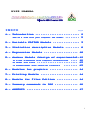
1
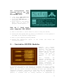
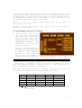
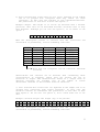
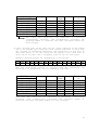
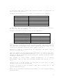
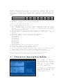
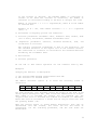
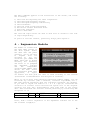
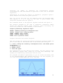
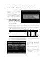
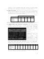
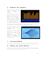
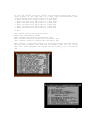
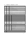
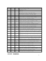
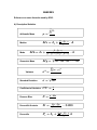
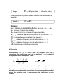
USER MANUAL INDEX Page 1.1.- Introduction ........................ ......................... 2 How do I load onto your computer SDG ATARI? ....... ........ 3 2.2.- Variable EDITOR Module ............... 3 3.3.- Statistics descriptive Module ........ 8 4.4.- Regression Module ................... 10 5.5.- Andeva Module (design of experiments).12 experiments).12 a) Fixed Treatments Treatments with complete randomization b) Model full block .... 12 ....................... 13 c) Random Model with factorial structure ........ 13 6.6.- Modules for for graphics ................ 14 7.7.- Printing Module ..................... 14 8.8.- Module for Files Edition ............ 14 9.9.- Summary commands in SDG ............. 16 A.- ANNEXES ANNEXES ............................. 17 1 1.- Introduction Graphs and statistics (SDG) is a powerful software and easy to use. Through menu you can create and edit variables, manage files, describe variables in statistical form, perform simple and multiple regression, analysis of variance for experimental designs, two-dimensional and three-dimensional graph equations, build scatter diagrams and histograms. It may also generate random variables, transform variables, variables to convert various formats to interact with various programs, create pie charts, bar, etc. All results are easy to interpret and the user requires only minimal knowledge of statistics. SDG consists of several modular programs that interact with each other through interactive menus with the user. All modules are scheduled in TURBO BASIC with some subroutines into machine code that makes some processes more efficient. All programs are unprotected and can be listed and or modified. With SDG you can graph their monthly expenses, statisticians calculate averages and other complexes, pooling their data in tables and get immediate histograms, to differentiate between products, predicting its sales or expenses, graph complex mathematical functions, and so on. The configuration physical ATARI: that requires you to use SDG in a 1) A computer ATARI with a minimum of 48 Kb RAM. 2) A floppy drive ATARI 3) A diskette SDG (A and B sides system or two separate floppy disks) with modular programmes. 4) A blank floppy disk to store files: variables (data), graphics, tables, etc. 5) A printer EPSON RC-220 or equivalent, optional. 6) An optional graphics. printer plotter ATARI 1020 for three-dimensional 2 The configuration that requires you to use SDG in emulation with Atari800Win Plus: 1) Load Image SDG-side-A.atr in the Disk Drive 1 2) Load Image SDG-Data.atr in Disk Drive 2 3) Reset emulator and disable BASIC. When you start the program, choose Option 2 How do I load onto your computer SDG ATARI? 1) Turn on the drive 1 (and 2 drive in case of using two Drives) 2) Insert the SDG system disk by side A (or Diskette 1 if the system is recorded in two separate floppy disks). 3) Turn on your computer pressing OPTION 4) Choose the appropriate instructions below. option on the screen and follow the 2.- Variable EDITOR Module Purpose: To create, modify or add data from a variable. The variables must be created or modified one by one, and before editing another variable, the above is recorded on the disk data. Once released all relevant variables, the modules can be used for descriptive statistics, graphs, regression, or analysis of variance for design of experiments. To increase the speed in the edition of variables and allow a greater degree of automation in the subsequent analysis of information, the editor lets you create variables according to their type (discrete or continuous variable), and agree to form that will be transferred to computer (or many variables with little data to be repeated). In general, a variable that is usually discreet is represented by 3 categories or classes only because it makes no sense to establish ranks continued with their values. The variables are considered continuous if it makes sense to group their values range or ranges. However, even if the variable is discreet, can be classified as if it were ongoing when the number of different values is very high. Options 1 and 3 are similar, introduced or edit data. they differ only in how they are Options 2 and 4 are similar, introduced or edit data. they differ only in how they are The SDG EDITOR distinction between: a) Data isolated with values that are very repeated in the sample and to be grouped into categories with only tables (no class intervals). In this case the variable is considered Discrete. The publication of such data is done with option 1 Example: Variable daughter. The number of children from 27 families. As we enter the 27 data of this variable (daughter), it is easier to enter using the OPTION 1 program, ie variable discrete values with repeated. 2 2 2 2 3 1 1 2 3 2 1 2 3 2 1 2 3 0 2 2 0 0 0 2 1 1 1 Note that the value 0 has a frequency of 4, the value 1 a frequency of 7, the value 2 a frequency of 12, and worth 3 a frequency of 4, ie, with many repeated values. 1 with the option of SDG facilitates the entry or editing of this type of variable. When the descriptive process of variable with SDG (tabulation calculation of parameters), will be something like this: Daughter 0 1 2 3 Totales Frequency 4 7 12 4 27 Frec. Acum. 4 11 23 27 - Frec. % 14.81 25.93 44.44 14.81 100 and Frec.Acum. % 14.81 40.74 85.19 100 - Note that the categories are not intervals (Discrete Variable) 4 b) Data isolated with values that are not (very) repeated in the sample and to be grouped into categories with only tables (no class intervals). In this case the variable is also considered Discrete. The publication of such data is done with Option 3. Example: Height. The height of 13 floors (m) measures with a decimal precision. Note that can be described discrete variables even if they have decimals. Although you can also use option 1, it is easier to use option 3 1.6 1.5 1.5 1.7 1.8 1.7 1.0 1.5 1.8 1.0 1.3 1.7 1.7 When the descriptive process of variable with SDG (tabulation calculation of parameters), will be something like this: HEIGHT 1.0 1.3 1.5 1.6 1.7 1.8 Totals Frecuency 2 1 3 1 4 2 13 Frec. Acum. 2 3 6 7 11 13 - Frec. % 15.38 7.69 23.08 7.69 30.77 15.38 100 and Frec.Acum. % 15.38 23.08 46.15 53.85 84.62 100 - Note that the categories are not intervals (Discrete Variable) Observations: The variable can be discreet when considering their classification in frequency tables does not involve the use of intervals or ranges. The classification tables in a unique class of discrete variables are possible only if the number of values "different" observed in the variable does not exceed 20. c) Data isolated with values that are repeated in the sample and to be grouped into categories with tables intervals. In this case the variable continue is considered. The publication of such data is done with Option 2. We can also use option 4, but I would write one to one data. Example: Variable weight. The weight (kg) of 40 persons: 45 45 45 50 50 52 40 50 48 48 38 45 50 40 50 45 45 50 37 37 45 37 37 39 50 37 42 48 45 45 45 50 52 37 37 45 45 45 48 38 When the descriptive process of variable with SDG (tabulation calculation of parameters), will be something like this: and 5 WEIGHT (kg) Lim. Inf. - Lim. Sup. 36 ≤ x ≤ 39 39 < x ≤ 42 42 < x ≤ 45 45 < x ≤ 48 48 < x ≤ 51 51 < x ≤ 54 Totals Average Frecuency 37.5 40.5 43.5 46.5 49.5 52.5 - 10 3 13 4 8 2 40 Frec. Acum. 10 13 26 30 38 40 - Frec. % 25.00 7.50 32.50 10.00 20.00 5.00 100 Frec.Acum. % 25.00 32.50 65.00 75.00 95.00 100 - Note that the categories are expressed by intervals (continuously variable). SDG automatically calculates the required number of intervals and lower and upper limits for each category. d) Data isolated with values that are not (very) repeated in the sample and to be grouped into categories with tables intervals. In this case the variable is considered Continuing. The publication of such data is done with Option 4. It also could use the option 2 but would have to write one to one data over a frequency value of one for each input. Example: Variable height (in centimeters) of 30 persons: 146 155 145 167 178 177 160 145 178 180 173 157 177 165 171 148 175 165 176 149 150 162 163 166 147 151 154 177 157 152 When the descriptive process of variable with SDG (tabulation calculation of parameters), will be something like this: HEIGHT (cm) Lim. Inf. - Lim. Sup. 145 ≤ x ≤ 151 151 < x ≤ 157 157 < x ≤ 163 163 < x ≤ 169 169 < x ≤ 175 175 < x ≤ 181 Totals Average Frecuency 148 154 160 166 172 178 - 8 5 3 4 3 7 30 Frec. Acum. 8 13 16 20 23 30 - Frec. % 26.67 16.67 10.00 13.33 10.00 23.33 100 and Frec.Acum. % 26.67 43.33 53.33 66.67 76.67 100 - Note that the categories are expressed by intervals (continuously variable). SDG automatically calculates the required number of intervals and lower and upper limits for each category. 6 e) The data come from a table with discrete classes or categories. In this case use the Option 5. Example: Classification of the number of children in 100 families: Number of children Clase 1: 0 Clase 2: 1 Clase 3: 2 Clase 4: 3 Clase 5: 4 Clase 6: 5 Number of families (frecuency) 12 33 30 15 8 2 f) The data come from a table with classes or categories of intervals. In this case the use OPTION 6 Example: Classification of salaries of 300 employees.: SALARIES Lim. Inf. Lim. Sup. Clase 1: 0 ≤ x ≤ 20000 Clase 2: 20000 < x ≤ 40000 Clase 3: 40000 < x ≤ 60000 Clase 4: 60000 < x ≤ 80000 Clase 5: 80000 < x ≤ 100000 Number of employees (frecuency) 100 80 70 30 20 Observations: The module Descriptive Statistics processed properly only when all these tables have equal intervals breadth. The upper limit of the intervals is included in each class, however the lower limit of the intervals is excluded from each class, except in Class 1. Options 1, 2 and 3, 4 respectively, are equivalent and differ only in how you can enter data. When the module is used descriptive statistics to analyze the data, must be chosen carefully between options 1, 2, 3, 4, 5 or 6, because it depends on which tables are incorporated into classes resulting unique or Ranges (Intervals). The modules to build chart, making regressions, or to design experiments, they can only use variables entered with options 1, 2, 3 or 4. Options 1 to 6 of the editor of variables are used only to enter variable (data) through the keyboard. Option 7 is used to edit variables taped drive through any of the options described above, Note: If you mistakenly entered the publisher, to leave him with enough pressure <Esc>. 7 Example: Enter through the editor the following variables (will be used later to exemplify processes). As there are few data and are not repeated, use option 3 of the publisher. There are two variables: An independent variable YEARS (YEARS) and a dependent variable production (PROD): Var1: Var2: YEARS PROD 2000 5 2001 10 2002 2003 2004 2005 2006 2007 165 25 38 52 68 84 To edit the variables above, follow these steps: 1) Turn on the drive Atari 1050 2) It floppy system by the side A 3) When the home screen of SDG, 1 choose whether their data are saved on a diskette that will drive the 1 (exchange with the floppy System), or 2 if their data is saved on a diskette that will drive the 2 (Another floppy 1050). 4) When displayed the main menu, choose Option 1 (EDITOR variable). 5) Choose option 3 Editor Variables (Keyboard - Discretos - not to repeat). 6) Enter the number of data containing the variable: 8. 7) Enter the data for one to one variable YEARS: 2000<return> 2001<return> 2002<return> 2003<return> 2004<return> 2005<return> 2006<return> 2007<return> 8) Check your data and verify they are correct. 9) Accept the income of the variable (Press A) 10) Insert the disk data and press <return>. 11) If you have not created variables that floppy, the directory will appear empty. Press "E" to finish watching the directory. 12) Enter the name of the variable: write YEARS and press <return>. Repeat entire process prior to the variable PROD (Production). Finally, return to the main menu by pressing <return>. 3.- Statistics descriptive Module This module can describe any statistically variable hospitalized with options from 1 to 6 Editor variables. Handing the following information: a) Table of frequencies with complete and absolute frequency percentage, and accumulated partial . 8 If the variable is discreet, the maximum number of categories or classes is 20. When the variable is continuous, the number of intervals is calculated according to the Rule of Sturges, who said: Number of intervals = 1 + 3.3 * Logbase10(N), where N is the number of isolated data. Example: If N = 200, then number intervals = 1 + 3.3 * Logbase10 (200) = 9 b) Histograms of frequency partial and cumulative. c) Position parameters: Arithmetic mean, Geometric mean, median, mode (one or more), Percentiles, Minimum and maximum value. d) Dispersion parameters: Variance, coefficient of variation. Standard deviation, rank, and The variance calculated corresponds to that of the population, and the Standard deviation is the square root of the variance earlier. The coefficient of variation is calculated as the standard deviation divided by the arithmetic mean. e) Bias Pearson f) kurtosis percentile At the end of this manual specifies all the formulas used by SDG. Examples: Studying the behavior of descriptive: a) the variable PROD defined enteriormente with SDG b) The variable X as defined below. Use Editor variables variable X: (option 12.23 13.00 18.07 15.36 15.22 18.76 12.25 14.56 4) to enter the 17.23 12.22 22.34 34.24 17.23 16.33 following values of 26.21 18.78 11.09 16.00 18.45 23.67 For both variables, once recorded, insert the floppy on the side B and choose Option Descriptive (4B). Then follow the instructions on screen. When asked if he recorded the results and you answered yes, the original data will be recorded and ordered not ordered (as admitted). These data will be recorded as a screen and can only be read later with the printing module (7B). When the results appear on screen Module descriptive, they will be distributed over six screens, the first two for the table of frequencies, for the following parameters, and the last three for Percentiles. 9 The menu commands appears on the bottom line of the screen, and allows the following: 1) 2) 3) 4) 5) 6) 7) 8) Show from the beginning the table frequencies. Show Histogram Frequency Partial Show Histogram Frequency Cumulatively Show Parameters Show the first screen Percentiles Record six screens described above. Print the reultados. Exit to Main Menu The left and right arrows are used to move half of screens to the left or right respectively. To print or save the results, previously always press Option 1. 4.- Regression Module The module is loaded from the Main Menu B-side of the disk system. Insert the disk data and press <return>, you'll see that in diquete data are recorded by the two variables you: YEARS and PROD. Press "E" to finish watching the directory and enter as it prompted the dependent variable and the independent variable PROD YEARS. Then choose the menu screen the regression model most appropriate, or adjust all models and then pick the best of them according to the results (Coefficient of Determination and analysis of variance). While it can be done using multiple regression models simple, you can transform any variable (add a constant, calculate logarithms, etc.). And then perform regression with the variables processed. For example, if you want to adjust the model is Y = A + B / SQR (X) transforms the variable X as follows: first calculate the square root of the original variable and save this transformation with some name in the floppy data. Then transform the variable created previously by calculating the reciprocal of it. Notación Guardar como X Var1 SQR(X) Var2 (o var 1) 1/SQR(X) Var3 (o var2 o var 1) Later, make a linear regression of the dependent variable "Y" on the new variable "1/SQR(X)". 10 Virtually all models of equations are linearization through transformations. The same method is applicable to the case of multiple regression. Observation: To record the results of regression, pre-press option 1 which rewrites the screen and press option 6. Also you can see the chart all the sampling points and adjusted model with options 3, 4 or 5. Only you can save or print figure high resolution obtained with the option 5. The estimated values of the equation adjusted obtained with option 2. The graphics produced by the form of regression (regression simple charts and diagrams scatter graph functions) while increasing its resolution greater the time remaining on the screen. Graphics produced by regression simple: SELECT: amending intensity of background color. OPTION: changes color intensity points. START + SELECT: chart records. START + OPTION: graphic prints. START: back to previous screen. Graphics functions and scatter diagrams: When the graphic has reached the desired resolution pressures START and you'll see a menu on the bottom line of the screen that lets you: 1, 2 and 3: modify the intensity of background color, and border points respectively. 4: graphic record. 5: graphic print. 6: leave the graph. The possibilities are many delivery this module, and only practice with the different options will allow you to take full advantage. All screens are sufficiently interactive with the user. All programs are modular unprotected, so you can review and modify some of its characteristics. Any problem that has to run the programs, you can reset with SYSTEM RESET and re-run with RUN. 11 5.- Andeva Module (design of experiments) The module calculates and constructs the table Analysis of Variance (Andeva) to study the existence of significant differences between different treatments. You have the option of bringing their design of experiments to one of the following models: a) Fixed Treatments with complete randomization. This model is used when the treatments were randomly assigned to the experimental units. Example: Suppose you have four treatments (A, B, C and D) relating to four different drugs to combat disease. The drugs are tested in groups of people, repeating the process five times. The response of the drug was measured by calculating the percentage of people who Sanaa. The results were as follows: Treatment % of people who heal (5 repetitions for each drug) A 40 30 20 10 50 B 50 70 60 40 30 C 80 80 90 50 100 D 30 40 50 50 30 The Analysis of Variance helps us to determine with any degree of confidence (as proof F) if possible to say that the effects of drug A, B, C or D are significantly different. To solve this problem, you must enter each of the treatments through EDITOR variable SDG. In other words, you must create 4 variable data with 5 each. This can be used for instance option 3 Editor. After creating the variables in the data disc, go to the Main Menu, where Choosing 6, which bear the form of analysis of variance. Then choose 12 option 1 of the following menu that appears on screen (Model treatments fixed completely randomized). Put your floppy and enter data from one to one variable (treatments) released earlier. b) Model full block. When there is no uniformity for all experimental units, can be separated into blocks, each with characteristics uniform. So for example, a soil fertility of different stripes, each of the strips to form a bloc passes, and within each bloc, the experimental units are assigned randomly. Example Blocks Block I Block II Block III Block IV 1 2 3 4 3 2 4 6 8 10 Treatments 3 12 14 15 11 4 9 6 4 5 5 3 6 3 4 Similar to previous point, each treatment (1 to 5) should be paid in advance with Editor Variables, and then use the module Andeva. c) Random Model with factorial structure. When each treatment consists of the variation of 2 or more factors, the design has factorial structure. By example, if one takes 2 factors, the first with two different levels and the second with three levels, treatments will be trained 2 x 3 = 6. Example: Suppose that a trial is conducted with two fertilizers (A and B) to test its effectiveness in separately and together (interaction). Using three doses for each fertilizer (A1, A2, A3 and B1, B2, B3), the combination therapies will be formed among them: A1B1, A1B2, A1B3, A2B1, A2B2, A2B3, A3B1, A3B2 and A3B3 (3 x 3 = 9 treatments). Suppose you are four replicates per treatment, and results in production are as follows: PRODUCTION (ton/acre). 4 repeticions per treatment A1B1 A1B2 A1B3 A2B1 A2B2 A2B3 A3B1 A3B2 A3B3 2 3 1 2 4 3 2 5 4 6 4 2 4 3 2 1 5 3 7 5 4 8 4 8 4 3 5 4 6 5 8 7 10 4 8 10 The 9 treatments are paid in advance as variables through Editor Variables, and then uses the module Andeva. 13 6.- Modules for graphics The graphics are the most common statistical bar (simple and grouped) and circulars (sectoral or cakes). Any variable can be created with SDG graficada with this module, provided it is within their capabilities. The pie charts require a maximum of one variable, however, the bar allowed up to three variables (all with the same number of data for each figure represents a bar). These graphs can be recorded and printed on paper. This module also allows the variables are entering through the keyboard directly without passing through the publisher of variables. Another interesting option is to graph functions of three variables in threedimensional shape. Observations: These graphics capability are not creción the author of SDG. The bar charts and circulars come from the software "GRAFIQUELO", and threedimensional graphics are known as "Z_PLOTTER". These programs have been adapted to use modular SDG. 7.- Printing Module It serves to recover on the screen and / or any file printer (graphic or not) product of the process of recording them from any form of SDG. 8.- Module for Files Edition Lets see any floppy directory, rename, delete, protect or unprotect files. Also used to format disks. In other words, it avoids having to leave the DOS to conduct these operations. 14 It also has another option to convert the variables created with SDG in other formats of the same SDG or to make them interchangeable with other programs. This option allows the following: -- Make variables with DIF format to format SDG -- Make variables with SDG format to format DIFF -- Make variables with SDF format to format SDG -- Make variables with SDG format to format SDF -- Make variables with SDD format to format SDC -- Make variables with SDC format to format SDD Format: SDG: Format used by the program itself. DIFF: Data Interchange Format. SDF: Standard Data Format (Column pure data) SDD: Discrete Variable created with the Editor SDG SDC: Variable cpntinua created with the Editor SDG The transfer to DIF format makes the variables created with SDG can be used by other programs like VisiCalc for example. They can also create data with other programs and through the DIF format, can be caught by SDG. 15 9.- Summary commands in SDG Click 1 1 Click 2 1 Result in the Editor of Variables 1 2 1 3 1 4 1 5 1 6 1 7 Click 1 2 2 2 2 2 2 2 2 2 Click 2 D B R P E C C C C Click 3 1 2 3 4 2 C 5 2 C 6 Click 1 Click 2 Click 3 Create, edit and burn discrete variables with values that are repeated. Create, edit and burn continuous variables with values that are repeated. Create, edit and burn discrete variables with values that are not repeated constantly. Create, edit and burn continuous variables with values that are not repeated constantly. Edit and recorded discrete variables that are tabulated in frequency tables to be processed by the module Descriptive Statistics. Edit and recorded discrete variables that are tabulated in frequency tables to be processed by the module Descriptive Statistics. Edit any variable disk previously recorded through Module Editor Variables SDG. 3 D B 3 D C 3 T B 3 T C 3 T T Click 1 4 Result in the File Editor Displays directory of any disc Clears files of any disc. renames files from one disk Protects files from one disk Unprotected files from one disk Converts variables with DIF format to format SDG Converts variables with SDG format to format DIFF Converts variables with SDF format to format SDG Converts variables with SDG format to format SDF Converts admitted as discrete variables to be processed by the processor as continuing Description of SDG Converts admitted as a continuous variable to be processed by the processor as discrete Description of SDG Result in Gráphics Create Bar graphs, capturing data variables recorded in Disk. Create pie charts, capturing data variables recorded in Disk. Create Bar graphs, entering data directly from the keyboard. Create pie charts, entering data directly from the keyboard. Create thridimentional graphics to enter with the keyboard the function of three variables. Result in Graphics Process the variables entered with descriptive statistics. 16 Click 1 Click 2 Click 3 5 1 - 5 2 - 5 3 - 5 4 - 5 5 A 5 5 B 5 5 C 5 5 D 5 5 E 5 5 F 5 5 G 5 5 H 5 5 I 5 5 J 5 5 K 5 5 L 5 5 M 5 5 N 5 5 O 5 5 P 5 5 Q 5 5 R 5 5 S 5 5 T 5 5 U 5 5 V Results in Graphics, Regressions and tranformations. Graf Dispersion Diagram between two variables recorded in Disk Graf functions of two variables entered with the keyboard. Make simple linear regression between two variables recorded on the Data Disk. Make Multiple Linear regression between 2, 3, or 4 variables recorded on the Data Disk. Generates variables with random data. Generates another variable ordering growing data in the form of a variable saved on disk. Generates a variable adding a constant to another variable of data recorded on disk. Generates a variable multiplying a constant per another variable of data recorded on disk. Generates another variable bringing to power a variable data recorded on disk. Generates another variable adding one to one of the data of two variables recorded on disk. Generates another variable by subtracting one-one data recorded on disc of two variables. Generates another variable multiplying one-one data of two variables recorded on disk. Generates another variable dividing one-one data of two variables recorded on disk. Generates another variable by calculating the square root of the data variable saved in a disk. Generates optionally another variable calculating the natural logarithm of data variable saved in a disk. Generates optionally another variable calculating the Briggs logarithm of data variable saved in a disk. Generates another variable by calculating the reciprocal of the data variable saved in a disk. Generates another variable by calculating the absolute value of a data variable saved on disc. Generates another variable becoming zeros the negative values of a variable saved to disk. Generates another variable becoming -1 the negative values of a variable saved to disk. Generates another variable calculating Sin(x) to a variable data recorded on disk. Generates another variable calculating Cos(x) to a variable data recorded on disk. Generates another variable calculating ArcTan(x) to a variable data recorded on disk. Generates another variable calculating the whole party to a variable data recorded on disk. Generates another variable rounding to the decimal specified recorded in disk. Generates another variable calculating Exp(x) to a variable data recorded on disk. USER MANUAL 17 ANNEXES Reference on some formulas used by SDG: A) Descriptive Statistics 8 ! \3 Arithmetic Mean .œ 8 Q / œ P3 Median Q o œ P3 Mode 3œ" Geometric Mean R # JÐ3"Ñ 03 03 0Ð3"Ñ Ð03 0Ð3"Ñ ÑÐ03 0Ð3"Ñ Ñ †E †E 8 Q1 œ È B" † B# † B$ † † † B 8 8 Variance 5# œ ! ÐB3 .Ñ# 3œ" 8 Standard Deviation 5 œ È5# Coefficient of Variation GZ œ Pearson Bias Wœ Percentilic Kurtosis Oœ Percentile 5 . .Q 9 5 T(& T#& #ÐT*! T"! Ñ T< œ P3 !Þ#'$ < "!! 8JÐ3"Ñ 03 E V œ ÐL 312/< .+>+Ñ ÐW7+66/< .+>+Ñ Range Other measures of position can be obtained from percentiles, for example: U" œ T#& Quartile 1 Notation: B3 À values of a variable Ð.+>+Ñ À B" ß B# ß B$ ß ÞÞÞß B8 8 À Number of data in the variable P3 À Lower Limit in the i-interval of frequencies table. JÐ3"Ñ À absolute frequency accumulated in the interval Ð3 "Ñ 03 À absolute frequency parcial in the interval Ð3Ñ 0Ð3"Ñ À absolute frequency parcial in the interval Ð3 "Ñ 0Ð3"Ñ À absolute frequency parcial in the interval Ð3 "Ñ E À Size intervals of the frequencies table A) Regression If the model ˜ œ ! " B %, then + and , are estimators of ! and " respectively. The coefficients + and , of the equation ] œ + ,B obtained using the method of least squares. Thus: 8 8 8 8 3œ" 8 3œ" 3œ" 3œ" 8! ÐB3 C3 Ñ! B3 ! C3 ,œ 3œ" 8! B#3 Ð! B3 Ñ# + œ ] ,\ In a similar manner calculated parameters in multiple linear regression. The variance analysis for regression is used to determine the extent to which the regression model used explains the phenomenon being studied across the variables used. It also measures the significance of each variable. The value of F calculated to be compared with the value of … Snedecor in the distribution of probabilities F given in statistical tables in books. We must employ the necessary degrees of freedom (given in the analysis of variance), and a confidence level desired (90, 95 or 99%). If the value of F calculated on the analysis of variance is greater than the F to the table of probabilities, then the ratio is significantly different from zero, ie should be part of regression model. The variance analysis to design experiments is studied in a similar manner, except that in this case is discussed if there are significant differences between treatments, or between factors if the design has factorial structure. In the latter case shows whether or not there is significant contributions of the various factors and their interactions in the response observed in the experiment.