Download User manual in PDF format - Kovach Computing Services

Oriana
Version 4
Users’ Manual
© 1994-2011 Kovach Computing Services, All Rights Reserved
Published by Kovach Computing Services, Pentraeth, Wales, U.K.
Last revised October 2011
Oriana - Copyright © 1994-2011 Kovach Computing Services. All Rights Reserved.
LIMITED USER LICENCE
Kovach Computing Services ("the licensor") grants the purchaser ("the licensee") a licence for the
computer program Oriana ("the program"), in accordance with the terms and conditions contained in
this agreement. The program is owned by us and is protected by copyright law, and we reserve
ownership of all Intellectual Property Rights in it, and all rights other than those expressly granted
by this Agreement.
The program is licensed for use by one user. The program may be transferred between computers or
users, so long as there is NO POSSIBILITY that the program will be used by more than one user at
any one time. The licensee may make additional copies of the software for archival purposes only. Any
accompanying printed user documentation may not be copied in any way. You must keep any
activation or registration code provided to you confidential. You must take reasonable steps to
protect the Software from unauthorised copying, publication, disclosure or distribution.
The licensee shall not use, copy, rent, lease, sell, modify, decompile, disassemble, otherwise reverse
engineer, or transfer the licensed program except as provided in this agreement. Any such
unauthorised use shall result in immediate and automatic termination of this licence.
This licence is non-transferrable and non-exclusive. Kovach Computing Services warrants that it is
the sole owner of the software and has full power and authority to grant the site licence without the
consent of any other parties.
LIMITED WARRANTY
Kovach Computing Services warrants the physical diskettes and physical documentation provided
under this agreement to be free of defects in materials and workmanship for a period of sixty days
from the purchase.
KOVACH COMPUTING SERVICES SPECIFICALLY DISCLAIMS ALL OTHER WARRANTIES OF
ANY KIND, EXPRESSED OR IMPLIED, INCLUDING BUT NOT LIMITED TO ANY WARRANTIES
OF MERCHANTABILITY AND/OR FITNESS FOR A PARTICULAR PURPOSE.
The total liability of Kovach Computing Services for any claim or damage arising out of the use of
the licensed program or otherwise related to this licence shall be limited to direct damages that shall
not exceed the price paid for the program.
IN NO EVENT SHALL THE LICENSOR BE LIABLE TO THE LICENSEE FOR ADDITIONAL
DAMAGES, INCLUDING ANY LOST PROFITS, LOST SAVINGS OR OTHER INCIDENTAL OR
CONSEQUENTIAL DAMAGES ARISING OUT OF THE USE OF OR INABILITY TO USE THE
LICENSED PROGRAM, EVEN IF LICENSOR HAS BEEN ADVISED OF THE POSSIBILITY OF
SUCH DAMAGES.
This agreement does not affect your statutory rights. The agreement shall be interpreted and
enforced in accordance with and shall be governed by the laws of England and Wales.
Contents
II
Table of Contents
Introduction
Part I - Introduction
Part II - Getting Started
0
1
3
1
2
3
What
.....................................................................................................................
is Oriana?
3
KCS
.....................................................................................................................
Desktop Metaphor
4
Oriana
.....................................................................................................................
Concepts
12
29
Part III - Tutorial
1
2
3
4
5
6
7
8
9
10
11
12
13
14
15
16
17
18
19
20
21
22
23
Creating
.....................................................................................................................
a data file
29
Entering
.....................................................................................................................
data
30
Selecting
.....................................................................................................................
spreadsheet cells
32
Editing
.....................................................................................................................
data
34
Entering
.....................................................................................................................
frequency data
36
Saving
.....................................................................................................................
data
38
Opening
.....................................................................................................................
an existing data file
38
Importing
.....................................................................................................................
data
39
Calculating
.....................................................................................................................
statistics
41
Selecting
.....................................................................................................................
a subgrouping variable
43
Filtering
.....................................................................................................................
data
44
Comparing
.....................................................................................................................
samples
45
Plotting
.....................................................................................................................
graphs
47
Adjusting
.....................................................................................................................
graph axes
49
Customizing
.....................................................................................................................
graphs
51
Saving
.....................................................................................................................
the desktop
54
Stacked
.....................................................................................................................
histograms
54
Two-variable
.....................................................................................................................
histograms
55
Circular-linear
.....................................................................................................................
plots
57
Printing
.....................................................................................................................
graphs and results
58
Saving
.....................................................................................................................
graphs and results to file
59
Changing
.....................................................................................................................
variable type
59
Summarizing
.....................................................................................................................
data
60
63
Part IV - Analyses
1
2
3
4
Statistics
..................................................................................................................... 63
Multisample
.....................................................................................................................
Test
71
Correlations
..................................................................................................................... 75
Second
.....................................................................................................................
Order Statistics
76
79
Part V - Graphs
1
2
3
4
5
6
7
8
9
10
Rose
.....................................................................................................................
Diagrams
79
Circular
.....................................................................................................................
Histograms
81
Raw
.....................................................................................................................
Data Plots
81
Arrow
.....................................................................................................................
Graphs
83
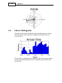
Linear
.....................................................................................................................
Histograms
84
Stacked
.....................................................................................................................
and Stepped Histograms
85
Two-variable
.....................................................................................................................
Histograms
86
Circular-linear
.....................................................................................................................
Plot
87
Distribution
.....................................................................................................................
Plots
88
Two-sample
.....................................................................................................................
Graphs
89
91
Part VI - Menus
1
File
..................................................................................................................... 91
III
Oriana 4
2
3
4
5
6
7
8
Edit
..................................................................................................................... 101
Data
..................................................................................................................... 105
Analyses
..................................................................................................................... 120
Graphs
..................................................................................................................... 127
Options
..................................................................................................................... 147
Window
..................................................................................................................... 153
Help
..................................................................................................................... 155
157
Part VII - Technical Support
1
2
Technical
.....................................................................................................................
support
157
Further
.....................................................................................................................
reading about circular statistics
158
159
Part VIII - Appendices
1
2
3
4
5
Drag
.....................................................................................................................
and Drop
159
Using
.....................................................................................................................
the keyboard
159
ISO
.....................................................................................................................
8601
160
Data
.....................................................................................................................
file structure
161
Example
.....................................................................................................................
data files
165
Index
167
Introduction
1
1
Introduction
Welcome to the manual for Oriana, the circular statistics
program for Windows. This manual will explain how to use the
program, what each menu item does, and gives some
background about the statistical analyses and graphs.
The first section, entitled Getting Started, explains the
structure of the program, while the second is a tutorial. To get
the most out of the program you should work through the
samples in the tutorial.
Throughout the text you will encounter symbols like this:
.
These symbols are page references. They point you towards the
section of the manual that gives you more information about
the term or concept that you have just read.
We hope that you find Oriana useful.
Suggested Citation
If you have used Oriana in study that you are publishing, the
following is a suggested format for the citation:
Kovach, W.L., 2011. Oriana – Circular Statistics for Windows,
ver. 4. Kovach Computing Services, Pentraeth, Wales, U.K.
We are always interested to see how Oriana is being used. We
would appreciate receiving reprints of any papers you have
published in which Oriana was used for data analysis. Thank
you!
Address for Correspondence
Kovach Computing Services
85 Nant-y-Felin
Pentraeth, Anglesey LL75 8UY
Wales, U.K.
E-mail: [email protected]
Web: http://www.kovcomp.com/
Tel.(UK): 01248-450414, (Intl.): +44-1248-450414
Fax (UK): 020-8020-0287, (Intl.): +44-20-8020-0287
Note: Please see the technical support section of this manual
before contacting us for technical support.
2
Oriana 4
We also maintain a mailing list for notifying customers of new
programs and other items of interest. It is a low volume list,
with at most one or two messages a month.
To join the KCS-ANNOUNCE mailing list send an e-mail
message to:
[email protected]
with the following text as the subject or first line of the body of
the mail message:
subscribe kcs-announce
Getting Started
2
Getting Started
2.1
What is Oriana?
3
Oriana is a program for Microsoft Windows that analyzes
orientations and other circular data. It will calculate a variety of
the special types of statistics necessary for working with data
measured in degrees, time of day or other circular scales. It will
also graph the data in a number of different ways.
Oriana will calculate basic statistics 63 such as the circular
mean and median, various measures of circular dispersion such
as mean vector length (r), concentration and circular variance
and standard deviation, along with confidence intervals for the
mean. A number of single-sample statistics are available for
testing whether the data adhere to uniform or other
distributions. There are also several multisample tests for
determining whether two or more samples differ significantly
from each other. Finally the program can calculate correlations
between circular samples as well as between sets of circular and
linear data.
A number of graph types 79 are available for plotting the data.
These include variants of the histogram for circular data,
including rose diagrams, circular histograms, linear histograms
and arrow plots, plus raw data plots and vector plots for circular
data. There are also distribution plots for comparing data to
theoretical distributions, Q-Q plots for comparing the
distributions of two samples, and scatterplots for plotting
circular as well as linear data.
Oriana has powerful data handling capabilities. It can work
with a variety of circular data types 13 in their native formats:
these include angles, time, day of the week, month, day or week
of the year, and compass directions. You can also include any
type of linear numerical data (for example if you wish to record
both wind direction and speed, or direction of movement of an
animal and distance traveled), which can then be used in some
of the graph types and in the circular-linear correlation. You can
also include full dates (which can later be summarized into the
various circular types) and labels for each observation. There is
also a subgrouping data type which allows you to assign each
data point to one of the groups you define, so that you can
analyze each subgroup separately as well as all data together.
4
Oriana 4
Data can be entered in a spreadsheet form, with separate
columns for each set of data or each variable, as well as in the
form of a frequency table. Data sorting, automated filling of
data, and search and replace facilities aid in entry and
maintenance of your data.
Oriana is designed to be as easy to use as possible and to be
compatible with all your other Windows applications. It closely
follows the modern Windows standards for menu structures and
the behavior of the Windows elements. It also allows you to
easily move data, results and graphs between Windows
programs, so that you can paste data from another application
into Oriana or transfer a table of results and a graph into your
word processor. Oriana also tailors itself to the way you work, so
that your favorite program options are saved automatically and
reinstated later. You can also save whole sets of graphs and
results using the KCS Desktop Metaphor 4 , allowing you to
return to work at the point where you left off.
This program is meant to be a tool rather than a teaching
program; this manual does not purport to teach you about
circular statistics. You should make sure you understand the
basic theory and assumptions behind the methods presented in
this package. There are a number of good books and papers
listed in the References 158 section that will help you in
learning about these methods.
2.2
KCS Desktop Metaphor
Oriana uses the KCS Desktop Metaphor. You can spread out
your data, the statistical results and the graphs in front of you
while you study them, just like paper on your desktop. Each
“piece of paper” is collected into notebook-like windows, one for
graphs and one for results. These have tabs to access each page.
There is also a notepad window that allows you to keep notes
about the analyses you are performing. All these windows are
contained within the main Oriana program window and they all
relate to a single data file.
The windows can each be resized, minimized, or moved around
while you study them and generate new pages. Each page can
then be printed and/or saved to a file if desired.
You can save your desktop to a file using the File|Save
Desktop command; later you can restore it to the same state,
Getting Started
5
using File|Open Desktop, so each window is just where you
left it with the same contents as before. You can continue
working where you left off. Multiple desktops can be saved for
different projects.
2.2.1
Windows
The Oriana desktop can have a number of different types of
windows open at any one time. These types of windows have
different appearances and characteristics, depending on their
function. In most cases you need not worry about these
differences. For example choosing the “Print” option will print
the currently active window, no matter what type it is; you will
notice no difference in the procedure.
The different windows automatically save their characteristics
for future use. For example, if you resize the status window so
that it is small and place it in the lower right corner, new status
windows will always be that size and position. Other types of
windows can have their own default size and placement.
Similarly, each type of window has its own characteristic font
147 and each can be set up to print to a different printer. 100
2.2.1.1
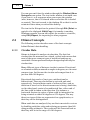
Main window
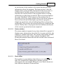
The Oriana program interface consists of a single main window
(a so-called multiple document window). A number of windows
can be displayed within this main window, as shown below.
All these windows relate to a single data file; if you wish to have
data and results from a second data file on your screen you can
run Oriana again to create a second main window.
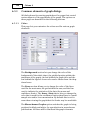
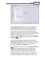
The image below shows a typical layout of the main window
during an analysis session.
6
Oriana 4
Note that most of the commands from the menus are also
represented as buttons on the toolbars at the top and left hand
side in the image above. These toolbars can be customized to
show just the buttons you want, and can be positioned anywhere
you would like.
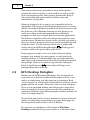
There are eight different toolbars that you can display, one for
each top level item in the main menu. You can choose which
toolbars to display by right clicking the mouse in an empty area
next to one of the toolbars and clicking on the name of the
desired toolbar. The buttons displayed on each toolbar can be
customized by clicking on the downward pointing triangle on
the right hand side of the toolbar, hovering the mouse over the
“Add or Remove Buttons” item, then over the toolbar name. A
list of all possible buttons for that toolbar will appear, with a
checkmark next to those that are visible. You can then click on
the items to check or uncheck the desired buttons.
The toolbars themselves can be moved around by clicking and
holding the mouse on the bar at the left end of the toolbar
(indicated above). The toolbars can be moved around to
different positions at the top or left hand side of the main
window, as shown above. They can also be placed on the right
hand side or bottom of the window by dragging them to those
positions. Finally you can drag the toolbar to float over the
center of the window, or float outside of the window.
Getting Started
7
At the bottom of the window is the status bar that provides
information about the program. The large section to the left
displays hints, giving a fuller description of the menu item or
toolbar button currently under the mouse pointer. It also
describes the current status of the program when it is doing
calculations or other long operations. The next section displays
the word “Modified” if the contents of the window that is
currently on top (the graph window above) have been modified.
Next to this is a button that lights up when the program is
doing long operations, such as loading large files or doing long
calculations. You can stop the current activity by clicking on this
button. Finally there is a progress bar that indicates how much
of the current operation has been completed.
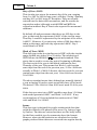
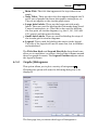
2.2.1.2
Status window
The status window is opened every time a data file is opened. It
displays some information about the file: its name and title, the
number of variables and cases, the current subgrouping variable
and defined vector pairs (if any), and the descriptive title.
Closing this window causes the data file and all other associated
files to be closed.
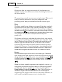
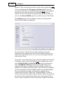
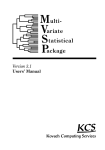
2.2.1.3
Data editor
This window is a spreadsheet that allows you to edit 34 your
data. The variables are displayed as columns, with the
observations for each sample filling the rows. Each column can
have different numbers of observations.
8
Oriana 4
The first row, headed Type, displays the data type for that
column. You can change the type of the data by simply clicking
on the down arrow labeled “Change data type” above.
The data are displayed in a format that matches the data type
12 . You can adjust certain aspects of the format, such as
number of decimal places or whether seconds should be
displayed, through the Options/Preferences 149 dialog box.
The display of certain data types, such as date or Day of Week,
will be displayed in your local format and language, as set up in
the Windows Control Panel.
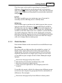
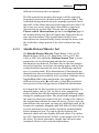
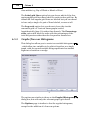
2.2.1.4
Results window
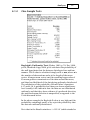
The results of the statistical analyses are displayed in a tabular
format in the Results window. This is basically a spreadsheet
and works in a similar way to the Data Editor, except that you
cannot change any of the values. Also this single window can
contain the results of many different analyses, each on different
pages. You can select the page you wish to view by clicking on
the tab along the bottom. Double-clicking the tab lets you
change the text on the tab.
Getting Started
9
The contents of this window can be saved using the File|
Export menu item when the window is the active window. The
results are written to the file in a tab-delimited plain text (i.e.
ASCII) format that can be read into any other program. The
columns will be separated by tabs, so that the alignment will be
preserved in any program that can interpret these tabs to form
a table.
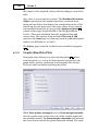
2.2.1.5
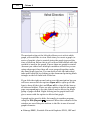
Graph windows
The graph window displays all the graphs so far produced, one
on each page. When you first create a graph 47 you can change
various settings that determine how the graph is drawn. You
can then modify the appearance of the graph by choosing the
Graph|Edit graph 147 menu item, or by right-clicking on the
graph and choosing Edit Graph.
The size of the graph can be changed by resizing the window.
Some of the graphs have a fixed length/width ratio, but the
shape of others can be adjusted by changing the shape of the
window.
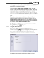
10
Oriana 4
The navigation bar at the left side allows you to select which
graph you would like to view. Each time you create a graph (or
series of graphs) a bar is created giving the graph type and the
time of creation. Below this is one or more tabs labeled with the
variable(s) used in the graph. If more than one graph is created
(because you either have multiple variables selected or you are
using subgroups) then these all occur grouped together under
the same graph type bar. You can show or hide the individual
tabs under each bar by clicking on the downward pointing black
triangle on the left hand side of the bar.
If you click the right mouse button over this navigation bar you
will see a menu with the options Open all (to open up all the
bars to show all the tabs) and Close all (to close all the bars so
all tabs are hidden). There are also options to delete the graph
page corresponding to the tab clicked, and to delete the whole
group of pages clicked. Right clicking on the graph itself will
give a menu with the option to delete that graph.
A graph can be saved to disk, for transfer to another program,
using the File|Export 97 command. When the contents of this
window are saved they are written to the file in one of several
graphic formats:
Bitmap (BMP), Portable Network Graphics (PNG), GIF and
Getting Started
11
JPEG (JPG) formats save the graph as individual pixels. The
resolution is limited to what you see on the screen. Note,
though, that the graph is saved at its current size, so if you
want a larger bitmap with higher resolution and fewer jagged
edges, increase the window to its maximum size. This format
can be edited in a painting type of program (such as the Paint
program included with Windows), but only on a pixel by pixel
basis.
The metafile formats (EMF and WMF) saves the graph as a
vector based drawing. This means that the graphic elements,
such as lines and circles, are saved as descriptions of those
elements rather than as a collection of pixels. Thus the graph
can be resized or printed in another program at the highest
resolution available. Also, the graph can be modified in a
vector-based drawing package. This would allow you, for
instance, to change the dashed line to a dotted one or change
the text of the labels.
The format used for saving the file is specified using the List
Files of Type option on the File|Export dialog box.
A graph can also be transferred to another program using the
Windows clipboard. Just choose the Edit|Copy menu item
when the graph window is the active window. You can then
switch to another program and use Edit|Paste to make the
transfer. Oriana places both bitmap and metafile versions of the
graph on the clipboard, so you can paste either one into your
other program.
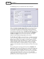
2.2.1.6
Notepad
The Notepad window provides a space for you to make notes
about the analyses you’ve done and any trends you’ve noticed. It
is a simple text editor with word wrap.
12
Oriana 4
You can open and close the window through the Window|Show
Notepad menu option. The text in the window is retained even
if you close it, so it reappears when you reopen the window
(note, however, that it is cleared when a new data file is loaded
or created). The text is saved to the desktop file so that it can be
reinstated later when you reload the desktop.
The text in the Notepad can be printed (through File|Print) or
copied to the clipboard (Edit|Copy) for transfer to another
Windows program You can also export the results to a text file,
using File|Export, for importing to other programs.
2.3
Oriana Concepts
The following section describes some of the basic concepts
behind Oriana’s data handling.
2.3.1
Circular Data
Oriana is designed to analyze circular data. The fact that
circular data are measured on a closed, cyclical scale means that
most of the more common types of statistical analyses are
unsuitable. Oriana performs analyses designed specifically for
circular data.
Many different types of data are circular in nature. Directional
or orientation data, measured as angles in degrees, are the most
common type. In this case the circular scale ranges from 0 to
just less than 360 degrees.
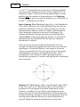
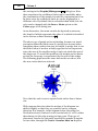
Directional data can be of two types, unidirectional or
bidirectional. These are also known as vectorial and axial
respectively. Vectorial data consist of a directed line, such as
direction of travel or the direction someone is facing. Axial data,
on the other hand, consist of an undirected line; either end of
the line could be taken as the direction. For instance, a
horizontal fracture in a piece of glass could be interpreted as
being oriented as either 90 degrees or 270 degrees. The way
these two types of data are represented on a graph varies, so
that they can be distinguished.
When axial data are analyzed, they are first converted to vectors
by doubling each data value and reducing any greater than 360
using modulo arithmetic. The results will be converted back so
that they will be in the range of 0-180 degrees.
Getting Started
13
There are other types of cyclical or circular data. Time of day is
another common type; with values measured on a closed scale
from 00:00 hours to 23:59 hours. Other variations on
chronological data can also be analyzed as circular data (e.g. day
of week, month of year, day of year, etc.)
Oriana has a wide range of native circular data types to match
the data with which you are working. There are also several
other non-circular data types for associating other data, such as
text labels or data measured on a linear scale, with your circular
data. You can find a summary of the data types in the section
entitled Oriana Data Types 13 .
When you create a new data file 29 , you specify the type of data
for each variable. You can later change the type of data in a
variable using the Data|Change data type 107 menu option.
2.3.2
Oriana Data Types
Each variable in an Oriana file is declared as one of 12 data
types. These determine the type of data that can be entered in
the data editor. The editor will restrict entry so that only valid
data can be entered. It also provides assistance in entering the
data, such as automatically entering the separators for times
and dates, or allowing you to enter day and month names from a
drop-down list or by typing just the first one or two letters.
The data types will also dictate how the data are handled
during analyses and graphing. For example, some data types are
inherently grouped (see section on Grouped Circular Data 26 ).
Oriana will automatically adjust graphs such as the rose
diagram to reflect the group width of the data (e.g. Month of
Year data will have 12 segments in the diagram, each 30° wide).
Some analyses cannot be reliably performed on grouped data,
and others must be adjusted to work properly, so Oriana takes
this into account.
Variables can be changed 59 between one type and another, but
data that do not fit into the range and assumptions of the
destination type may be lost or converted to nonsensical values.
The characteristics of the different variable types are listed
below.
14
Oriana 4
Angles
This is the basic circular type, where data are measured within
the range of 0°-360°. The data editor will not allow any values
outside of this range to be entered.
Occasionally researchers find it useful to measure angles as a
deviation from a home direction. So, for example, if the
expected direction of travel is 0°, and one subject travels 10° to
the left, then a value of -10° would be recorded. The Oriana
Angles variable type will not allow negative numbers to be
entered. However, you can get around this by entering the data
into a Linear variable (described below), which will accept
negative numbers. Once all data have been entered you can
change the variable type 59 to Angles. Any negative numbers
will be converted to the appropriate degrees (e.g. -10° will
become 350°).
Axial
This is similar to the Angles type, but the data are bidirectional
rather than unidirectional, as discussed in the Circular Data 12
topic above. Data can still be entered in the full 0°-360° range,
but when analyses are performed the data are doubled and then
back converted, so that they are within the range of 0°-180°.
Circular Proportional
This is also similar to the Angles type, but instead of entering
data in the range of 0-360 the data are entered as a proportion
of the whole circle, ranging from 0-1. So a value of 0.5 would be
the same as 180°. The range of 0-1 is also used for labeling
graphs and output.
Circular Percentage
This is like Circular Proportional, but the data are on a
percentage scale ranging from 0-100.
Compass Direction
This data type presents angular data as directions of the
compass. Data are entered into the editor as letters indicating
the direction (e.g. N for North, SW for South-west, NNE for
North-north-east, etc.). You can use up to 16 compass points
(including the three letter ones such as NNE) or restrict the
data to the four or eight main points (e.g. N or SW). Oriana will
automatically detect which you are using and adjust the
histogram bar widths and chi-square class widths accordingly.
Getting Started
15
The underlying data are still angular, and all calculations are
performed on and reported as angles. For mean and median
directions the corresponding compass direction is also reported.
The actual angle stored is the midpoint of the compass sector, so
North would be 0°, East 90°, South-east 135°, etc.
You can customize the abbreviations used for compass points (e.
g. NNE) to match your own preferences or local language
through the Options|Preferences 149 menu item.
Time
The Time data type presents the circular data as time in hours,
minutes and seconds on a 24 hour scale. The data can range
from 00:00:00 to 23:59:59 (or 12:00:00 AM to 11:59:59 PM).
The format used to display the time depends on the settings in
the Windows Control Panel.
As with other circular data, the data are stored as angles.
However, the mean and median times and the confidence limits
are reported as time values.
Day of Week (DOW)
This circular type divides the 360° range into 7 groups,
representing the seven days of the week. The order of the days
follows the ISO 8601 160 international standard, where Monday
is the first day and Sunday the last.
As with other circular data the underlying data are in angles,
with the midpoint of the sector being the angle stored. Each
sector is 360/7 or approximately 51.4286° wide, so the first day
has an angle of around 25.7143°, and day 7 is ca. 334.2857°.
Means and medians are reported in angles, but the associated
DOW is also reported. The actual text displayed in the results,
graphs and data editor are in the user’s local language, as set up
in the Windows Control Panel, so Monday is displayed for the
first day in English, Lunes in Spanish, etc. Currently Oriana
cannot properly display day names that do not use the Roman
alphabet.
Month of Year (MOY)
This data type works in a similar way to DOW, except it is
divided into 12 groups for the months of the year, with January
first and December last. Each sector is 30° wide, with January
being 15°, February 45° and December 345°.
16
Oriana 4
Day of Year (DOY)
This circular type stores the numeric day of the year, ranging
from 1 to 365 (or 366 for leap years), with day 1 being 1 January
and day 365 (or 366) being 31 December. They are actually
entered into the data editor as numbers, and the results are
reported as angles (although, as with DOW and MOY the
equivalent numeric Day of Year is also reported for means and
medians).
By default all analyses assume that there are 365 days in the
year, so that each day represents 0.9863° of the circular range.
Thus Day 1 would be represented by the midpoint of the sector,
0.49315°. However, if you enter any values of 366 then that is
taken as the range, and each day represents 0.9836°. Day 1
would then be 0.4918°.
Week of Year (WOY)
This data type works in a similar way to DOY, with the circular
range divided into either 52 or 53 weeks. The calculation of
WOY follows the ISO 8601 160 international standard. This
states that a week is a seven day period, beginning on Monday.
The first week of the year is that which contains the first
Thursday of the year. This means that Week 1 could contain
some days from the end of the previous year; 31 Dec. 2002 was
actually in Week 1 of 2003. Likewise, the last week of a year can
contain some days from the next year; 1 Jan. 2000 was in week
52 of 1999.
The above standard means that, although we normally think of
a year as having 52 weeks, some can actually have a 53rd week.
The dates 27 Dec. 2004 to 2 Jan. 2005 were week 53 of the year
2004.
If the data you enter into a WOY variable range from 1-52 then
each week represents 6.9231° and Week 1 is 3.4615°. If any
week numbers of 53 are included then each week is 6.7924°
wide and Week 1 is 3.3962°.
Lunar
This data type is designed for people working with data that
might be related to the phases of the moon (e.g. laying of eggs
by turtles). The data are entered as dates (see the entry below
for the Date variable type for comments about the format).
However, when circular statistics are calculated or circular
graphs produced these dates are converted into angular data by
Getting Started
17
calculating the length of the lunar month and the day of the
lunar cycle. For example, a date of 3 April 2011 will be plotted
on a circular histogram at the top, in the 0° position, since that
is the date of a new moon, and 18 April 2011, a full moon day,
will be at the 180° position.
Note that all dates are based on the Gregorian calendar, in
accordance with ISO standard 8601 160 . This is the calendar
that was adopted in 1582 by the Vatican and many Catholic
countries, 1752 by the British Empire, 1918 in Russia, and
numerous other dates in other countries around the world. If
you are working with dates that were recorded under the Julian
calendar before these years they will need to be converted to the
Gregorian calendar for the moon phase to be calculated
correctly. This can be done by adding a certain number of days
depending on the date range. A table in the Wikipedia topic on
the Proleptic Gregorian Calendar gives the required number of
days.
Note too that you can specify the time zone in which the lunar
dates were recorded. The exact point in time at which the moon
phase becomes new or full is the same all over the world, but
because of differing times zones the clock time and perhaps the
date will be different. For example, a new moon occurred on 4
March 2011 at 20:46 UTC. Thus the date of the new moon
would have been 4 March in Great Britain. However, when that
new moon occurred it was 07:46 on 5 March in Sydney,
Australia. The difference in dates can affect how graphs are
drawn and statistics calculated.
By default Oriana will use the time zone specified in the
Windows system on which it is running (which can be changed
through the Control Panel or the clock on the Task Bar). If you
are regularly analyzing data from a different time zone you can
change the zone that Oriana will use through the Default
Time Zone option on the Lunar Phases tab of the Options|
Preferences 149 dialog. You can also change the time zone for
individual variables through the Data|Change Variable
Type 107 dialog. The time zone for each variable is saved in the
data file, so if you send the file to a colleague in a different time
zone the original time zone will still be used.
The Options|Preferences 149 dialog also allows you to
customize the names used for different phases of the moon.
These names are used on the graphs and the basic statistics
18
Oriana 4
output.
Please note that no correction is made for local summer or
daylight savings time differences when calculating the dates of
the moon phases.
The remaining variable types are non-circular types. They can be
used for labeling data cases, specifying subgroups, and
providing linear data for correlation with the circular types.
Date
The Date variable type allows you to specify the date on which
an observation took place. This could be auxiliary data, which
allows you to group your circular data observations according to
calendar periods. Or it could be your main data, which will later
be summarized 60 into circular types, such as days of the week
or months of the year, then analyzed statistically and
graphically.
The format of the date (including the order of the year, month
and day portions) follows that specified as the short date format
in the Windows Control Panel. Normally this would be an all
numeric type such as 2003-05-27, 27-05-03 or 05/27/2003.
Currently the data editor requires numeric format for direct
data input. However, if you are pasting or importing data from
another source that is in mixed format (such as 27 May 2003)
Oriana will recognize this and convert it to numeric format.
Linear
The linear data type can be used to store any type of numeric
data, both positive and negative. These data can then be plotted
along with the circular data on the two-variable histograms 138 ,
circular-linear plots 87 or the two sample scatter plots 145 , and
compared to the circular data with circular-linear correlation
125 .
When the linear variable represents the length of a vector (e.g.
wind speed or distance traveled) then you can define an angle
variable and a linear variable as a vector pair, through the
Data|Define Vector Pair 114 menu item. This allows you to
calculate weighted mean values (where the mean angle is
weighted by the length of the vectors) in the basic statistics, as
well as add a weighted mean vector to circular plots.
Getting Started
19
This data type is also used for specifying the frequency of
different values when data are being entered in a frequency
table format 22 , and for specifying the r value when means and
mean vector lengths are being input for second order statistical
analysis 76 .
Labels
The label variable type can contain any type of text and is
normally used for labeling cases to identify them.
Subgroup
This variable type is similar to the Labels type in that you can
type any text into it. However, it is specialized to be used for
dividing cases up into subgroups 43 , so that each subgroup can
be analyzed separately. When text is entered into a Subgroup
variable in the data editor that text is added to an internal list
of possible subgroups. That list can be displayed by using the
drop-down box that appears in every cell of a Subgroup variable.
You can use this drop-down box to enter new data into empty
cells, or to change that in existing ones.
2.3.3
Data Structure
Data within Oriana can be structured in several different ways.
Raw Data
The first is the one that was the sole method in version 1 of
Oriana. Here each column in the data editor represents an
independent collection of measurements. If all your data are
repeated observations of a single type of object or event then
you would have just a single column of data. Examples might
include:
Directions that pigeons fly after release
Orientation of tool marks in sedimentary rocks
Direction of wind at a single station
Time of arrival of patients at the emergency ward of a
hospital
You might also want to divide the data up into different groups
so that you can compare the groups and look for similarities or
differences. For example:
Directions that pigeons fly from different release points
20
Oriana 4
Orientation of tool marks in different strata of rock
Direction of wind in different months or seasons
Time of arrival of emergency patients on different days of the
week
In these cases you would have a separate column for data from
each release point, strata, month or day. Here is an example of
data of wind directions from each month. Notice that each
column can have different numbers of observations.
Paired Data
Oriana version 2 introduced a new method of structuring the
data that allows much more flexibility. With this new method
each column is a separate variable rather than set of
observations. You might have one column with all the
directional or time data, plus another with a variable that you
can optionally use to divide the data into subgroups. For
example, with the arrival time example above, the first column
would have all of the arrival times, and the second would have
the day that each arrival time was recorded. The data are
paired, so that each row of the data matrix gives all the data
about a single event. Here is the data matrix:
Getting Started
21
Row 1 records the arrival of a patient at 18:42 on a Sunday,
Row 2 records an arrival at 16:51 on Thursday, etc. With this
format you can, for example, produce a rose diagram of all the
arrival times, then produce a series of diagrams, one for each
day.
With data of this type each column must have the same number
of rows, since the data are paired. However, Oriana can handle
missing data, so if one of the variables doesn’t have data for a
particular observation you can just leave that cell blank. Oriana
will deal with the missing data in the most appropriate way for
the given analysis or graph. For example, if some of the values
in the Day column above are missing, then, when producing
graphs for each day, a separate graph will be produced for those
where the day is not known. Any missing circular data are just
ignored and not included in the graphs or statistics.
With this type of paired format you can also add other variables,
allowing you to subgroup the data in different ways, or to
correlate the circular data with other types of data. Here is an
example of some wind data:
22
Oriana 4
Here each row represents an hourly wind measurement. For
each observation we have recorded the date and time of the
observation, along with the wind direction at that time, the
wind speed, the temperature and atmospheric pressure. We can
now analyze all the wind direction data together. We can also
use the Date variable for grouping by various methods, such as
month of year, day of week or year. Finally, we can use the Wind
Speed variable to compare wind speed with wind direction. This
can be done with a two-variable rose diagram, 86 circular-linear
plots 87 or by circular-linear correlation 76 .
You can switch between having the data in the old Oriana 1
format and the new paired format with the Data|Change
Data Structure 109 command. See that section for more
details and restrictions. Also, when opening a file created with
the old Oriana version 1 you will be asked if you wish to convert
it to the paired format.
Note: with paired data it is most suitable to describe each
column in the data editor as a variable. However, with the
original Oriana version 1 method of structuring the data each
column is better thought of as a set of observations. Throughout
the program and this document the term variable is usually
used for each column, but in data sets using the latter method
of structuring the term set of observations can be substituted.
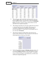
Frequency Data
Often data are collected or provided in the form of a frequency
table, where the number of times a particular direction was
Getting Started
23
observed is recorded as the frequency, for example:
Direction
Frequency
0.000
15
15.000
25
30.000
35
45.000
45
60.000
35
75.000
25
90.000
15
180.000
15
195.000
25
210.000
35
225.000
45
240.000
35
255.000
25
Oriana has two ways of dealing with data like this.
1. The first is a special data editing mode called Frequency
Editing, which allows you to enter and edit data in this
fashion. To enter data in this method you would first create a
new data file 29 as normal, then select a cell in the
appropriate column of the data editor and choose the Data|
Edit Frequencies menu command. This will open a dialog
box with a frequency table like the one above, allowing you to
enter the observations and their frequency. Once you are done
the column of the data editor will be filled with data
representing all the observations summarized in the
frequency table, in a single column.
2. You can also enter frequency data directly in the data editor.
To do this you need to have two variables, the first being one
of the circular types and the other a Linear type variable. You
can then enter the data in the same form as the table above,
as in this example:
24
Oriana 4
When this method is used for entering frequency data you
must specify that the data are in frequency format on the
Select page 120 of the Analyses or Graphs dialog boxes.
Note that the second method can only be used for basic
statistics and histograms. If you need to do multisample
comparison tests then you will need to use the first method, or
use Data|Change Data Structure to convert the frequency
table to raw data.
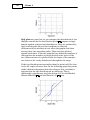
Deviation Data
Occasionally data are measured as deviations from a particular
direction. For example, it might be expected that bees would fly
in a particular direction, and observations are made of the
actual angle of travel compared to the expected. Thus some
observations might be negative numbers (flight to the left of
the expected direction) and others positive.
Oriana expects angular data to be in degrees ranging from 0360, so the data editor does not allow entry of negative data for
angular variables. However, this can be worked around by
entering the deviation data into a variable of the Linear type,
which allows numbers of any type. Once the data have all been
entered the type of the data variable can be changed 59 to
Angles. When this is done Oriana will automatically convert the
negative data to the equivalent on the 0°-360° scale. So -10°
would be converted to 350°. The following shows the data before
and after conversion:
Getting Started
25
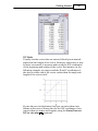
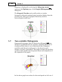
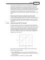
X/Y Data
Usually circular vector data are entered directly as measured
angles and the length of the vector. However, sometimes it may
be more convenient to measure and record the X/Y coordinates
of the beginning and ending of the vector. For instance, in the
following example you may record the X and Y coordinates of
the dots at either end of the vector, rather than the angle and
length of the vector itself:
If your data are in this format then you can enter them into
Oriana as four sets of linear data for the X/Y coordinates, then
convert them to angles and lengths, using the Data|Convert
X/Y to circular 111 command.
26
2.3.4
Oriana 4
Grouped Circular Data
Often circular data can be considered as grouped. This should
not be confused with grouping data into different subgroups
(such as arrival times on different days or wind direction in
different months). Grouped circular data means that the
observations have been recorded approximately, to the nearest
interval, rather than exactly. For example:
A rough approximation might be made as to direction of
travel (0°, 45°, 90°, 135°, 180°, etc.)
The direction might be recorded to the nearest 10° rather
than a more exact measure (e.g. 20° rather than 21.25°), or
time to the closest hour.
The data might be collated into a frequency table based on
intervals, such as 10 observations between 0° and 30°, 12
between 30° and 60°, etc.
Many of the Oriana circular data types are inherently
grouped. Day of Week has seven intervals, one for each day,
Month of Year has 12 intervals, and Compass Direction can
have four, eight or 16.
This can simplify data collection, but it can also cause problems
in data analysis. It can introduce a bias into the results, or
indeed can completely invalidate the statistical procedure.
Where possible Oriana will attempt to correct for this bias,
using recognized corrections or alternative calculations, but
some analyses simply cannot be calculated on these types of
data.
After you have entered or imported a new set of data, and before
saving or analyzing the data, Oriana will scan through them to
see if they appear to be grouped. If so, Oriana will prompt you
with a dialog box, asking if the data actually are grouped and, if
so, what the grouping interval is. If you confirm that the data
are grouped then Oriana will record this and will take the
grouping into account in all analyses. If you clear the Data Are
Grouped tick box then Oriana will remember this and will
always proceed as if the data are not grouped. You can change
this declaration later through the Data|Change Variable
Type 107 menu item.
2.3.5
Missing Data
Oriana can easily handle missing data. There is no need to enter
a special missing data marker; simply leave a cell in the
Getting Started
27
spreadsheet blank and Oriana will consider that data as
missing.
With all single sample statistics, tests and graphs the missing
data are ignored and not included in the results. With pairwise
tests missing data are handled by pairwise deletion (leaving out
any pair of data where one is missing). For multisample tests
listwise deletion is performed (any row that contains one or
more missing data is ignored).
Tutorial
3
29
Tutorial
The following topics give step-by-step instructions on using
Oriana.
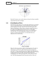
3.1
Creating a data file
The first step in using Oriana is to create a new data file. Do
this using the File|New command from the main menu. A
multi-step “wizard” dialog box will be displayed; this helps you
in setting up your data file. You will be asked various questions
about your type of data. For now let’s assume we just have one
set of circular data. You should:
1.
2.
3.
4.
5.
6.
7.
Choose Angles as the type of data you are working with,
then click on the Next button.
Choose the Separate option on the data layout page, then
click on Next.
Pick Circular data only and press Next.
Make sure Number of columns is set to 1.
Enter a label for this column of data in the Labels box and
press Next.
Enter a descriptive title for the file, then Finish.
The dialog will close and the status window 7 and data
editor 7 will appear.
Now you can start entering data. The data editor has a single
column for typing in the single set of data. New columns can be
added by simply pressing the left arrow key, or using the Edit|
Insert Column 104 command.
The spreadsheet will be empty except for two rows of grey cells
across the top. One contains the data type, the other the label
you entered in the New File wizard. Data can then be typed
into the main body of the spreadsheet. The following image
shows a new data matrix in which five data points have been
entered:
30
3.2
Oriana 4
Entering data
To begin entering data you must open the Data Editor 7
window, if it isn’t already. Do this by choosing Data|Edit Data
from the menu. A spreadsheet-like editor will appear. Initially
the cell in the upper left corner will have a dark line around it.
This is the active cell and is where any characters or numbers
that are typed will appear. You can move the active cell around
the spreadsheet, using the mouse to select a new one or by using
the arrow keys. Other keystrokes are also recognized for
navigating the spreadsheet; see the section on using the
keyboard 159 for a full list.
The spreadsheet has column headers labeled A, B, C, etc. and
row headers labeled 1, 2, 3, etc. These headers indicate the
position within the spreadsheet and also can be clicked to select
the whole row or column for editing purposes.
You can change the width of the columns and height of the rows
Tutorial
31
by using the mouse to drag the separator between the headers.
Normally each row or column is changed individually. However,
holding down the shift key while you resize a row or column
causes all others to be changed to the same size.
The first two rows are shaded. The first row contains the
indicator of the type of the variable. You can change the variable
type, say from Angles to Time, by clicking on the little arrow
next to each cell (labeled “Change data type” above) and
choosing a new type.
The second row contains the name of each variable. These labels
are used on the output to identify the variables or sets of
observations. New variables are by default given the same name
as their data type. You can change these by making the
appropriate cell active and typing any characters. Spaces may be
included and the labels may be up to 60 characters long
(although shorter labels allow you to keep the columns widths
narrow and see more data on the screen).
Typing in data
Once labels have been entered you can start typing in the
numeric data. This is done by making the appropriate cell
active and typing the numbers. You then press the Enter or Tab
key or the up or down arrow keys to finish entering the data;
the Enter key will also move the active cell to next cell down
ready to enter the next datum while the Tab key will move to
the cell to the right.
As you type in data, the values are checked to make sure they
are valid (e.g. in the range of 0-360 degrees or 00:00-23:59
hours). The program will beep and refuse to accept any values
that are not valid. Some data types, such as Day of Week, have a
fixed list of possible values. You can choose the desired entry by
clicking on the down arrow labeled “Change datum” in the
image above. You can also go straight to an entry by just typing
the first few characters of the desired entry.
With Date and Time cells a small scroller (labeled “Increment
Date” in the image above) will appear next to the cell when you
begin typing. You can use this to increment and decrement the
date or time. With Date cells, if you double click on the cell
when the scroller is visible a monthly calendar will be
displayed; you can pick a new date from this.
32
Oriana 4
You can close the data editor at any time by again selecting
Data|Edit Data from the menu (or clicking on its matching
button on the toolbar) or by clicking on the close button (the
one with the x) in the upper right corner. The data are
maintained in memory and will appear when you open the
editor again. They are not saved to disk yet, though. You can do
this by explicitly saving the data with File|Save Data. If you
try to exit the program or open/create a new file when the data
have not been saved you will be warned and asked if you wish to
save the data.
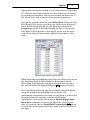
3.3
Selecting spreadsheet cells
Normally the spreadsheet will have a single active cell while
you are working on it. The active cell can be selected by
positioning the cursor (which is a
when it is over the
spreadsheet) over the desired cell and clicking the left mouse
button. Alternatively, you can move the selected box around
using the arrow keys.
This image shows the active cell in column A, row 2.
To select a number of cells (in preparation for deleting them or
copying them to the clipboard), you can simply hold down the
left mouse button and drag the cursor over the desired cells.
Alternatively, hold down the shift key while you move the
cursor with the arrow keys. The resulting selected block of cells
will look like this:
Tutorial
33
You can select whole rows or columns by clicking on the row or
column headers. Multiple rows or columns can be selected by
dragging the cursor across the headers. The current row can also
be selected by pressing Shift-Space; a column can be selected
with Ctrl-Space. The following images show the result (the
is positioned over the header that was clicked to perform the
selection):
34
Oriana 4
The entire spreadsheet can be selected by pressing the button
in the upper left corner of the spreadsheet. You can also select
the whole spreadsheet using the Edit|Select all command, or
by pressing Shift-Ctrl-Space. The result looks like this:
3.4
Editing data
There are a number of editing actions you can perform on
existing data.
Overwriting old data with new
Make the cell active (click with the mouse or move to that cell
with the cursor keys), type the new value, and press the Enter
key.
Modifying data within a cell
Make the cell active and press F2 (or double click on the cell
with the mouse). This will cause the contents of the cell to be
selected. Clicking again or press the right or left arrow keys will
cause a caret (vertical line) to appear. You can move this back
and forth with the cursor keys.
Any new letters or numbers typed will appear at the position of
the cursor. With labels, and the portion of numeric data to the
left of the decimal, the new characters will be inserted. With
the fractional part of numeric data the typed digits will replace
those at the caret (which will be shown as a triangle under the
digit).
Some variable types, such as Day of Week, have a fixed list of
possible data values. This list can be seen by clicking on the
down arrow button to the right of each cell (see below). The
Tutorial
35
entry for that cell can then be selected from the list. You can
also just start typing while the cell is active; the data editor will
automatically insert the data value that matches what you have
typed so far.
With time and date variables the separators between elements
of the data value are automatically included; there is no need to
type them.
Clearing data in one or more cells
Make the cell active and press the Del key, choose Edit|Delete
from the menu, or choose Delete from the context menu.
To clear several cells at once select the desired cells and use one
of the above commands.
Pasting data from the clipboard
Make active the cell at the upper left of where you wish the
clipboard contents to be pasted. Then choose Edit|Paste, press
Ctrl-V, or choose Paste from the context menu. The pasted data
will overwrite existing data.
The data will be validated as they are pasted to ensure they are
valid given the variable type. Any data that are not valid are
ignored and the cell remains blank. A warning will be displayed
if this happens. If the column into which you are pasting does
not yet have any data, then Oriana will try to guess the most
appropriate data type, given the data on the clipboard. If this
guess is wrong you can set the column to the appropriate type,
make sure there is data in at least one cell, then try pasting
again.
If the data in the clipboard contains more rows or columns than
will fit in the spreadsheet then more rows or columns will be
added automatically.
Adding new columns and rows
New rows or columns can be added singly by going to the last
cell in the row or column and pressing the right or down arrow
keys.
36
Oriana 4
To insert new rows or columns in the middle of the spreadsheet
select a whole row or column, then choose Edit|Insert Row/
Column (or Insert Row/Column from the context menu). To
insert two or more rows or columns select two or more existing
ones.
If Insert Row/Column is chosen when there are not any whole
rows or columns selected a dialog box will appear. This lets you
specify exactly what to insert.
Deleting columns and rows
To completely remove rows or columns from the spreadsheet
select a whole row or column, then choose Edit|Delete Row/
Column (or Delete Row/Column from the context menu). To
delete two or more rows or columns select two or more existing
ones. (Note - pressing the Del key while columns or rows are
selected will not remove them, but instead will delete their
contents).
If Delete Row/Column is chosen when there are not any whole
rows or columns selected a dialog box will appear. This lets you
specify exactly what to delete.
Reversing editing changes
The Oriana data editor keeps track of all changes you have
made. Changes can be undone, in the reverse order that they
were performed, by choosing Edit|Undo from the menu (or
pressing Ctrl-Z). The menu item and the hint on the status bar
at the bottom of the window will tell you exactly what change
will be undone next.
To reinstate a change that you have undone choose the Edit|
Redo menu item.
The list of editing changes is only maintained while the data
editor is open. If you close the data editor and reopen it you will
not be able to undo previous changes.
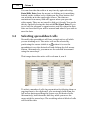
3.5
Entering frequency data
In most cases you will be entering raw data, the individual
measurements collected in your study. However, in some cases
you may be provided with data that are in the form of a
frequency table, where the number of measurements of each
Tutorial
37
unique data value are recorded (e.g. 25 observations of the angle
45°). Data in this format can also be entered directly in Oriana
by creating two variables, one for your circular data and one, of
the Linear type, that is used for entering the frequencies.
You can set up such a data file using Files|New. Using the New
File Wizard, first choose your data type, then on the next page,
where different data file layouts are described, choose the
Frequency option. Following through the rest of the wizard
will result in a file similar to that below, where you can enter
your data in the left-hand column and the frequencies in the
right.
When analyzing and graphing these data you will need to choose
the Frequency option (rather than the Raw option) on the
Select page of the analysis or graph dialog box. See the end of
the tutorial about Calculating Statistics 41 for more details.
Note that this method can only be used when calculating basic
statistics and plotting histograms. If you need to do
multisample comparison tests then you will need to convert the
frequency data into raw data (columns of individual
observations). You can do this using the Data|Change Data
Structure command to convert the frequency tables to raw
data. You can also use the Data|Edit Frequencies 106 option
to enter data as frequencies but have them saved as columns of
raw data.
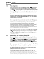
38
3.6
Oriana 4
Saving data
Data are saved through the File|Save Data 93 menu item. If
you have created a new data file (and the status window says
“Unnamed” for the filename) you will then be presented with a
Save As 93 dialog box. You can choose the appropriate disk and
directory, then type a name into the File name edit box and
press OK.
If the file already has a name (which will appear in the status
window) then choosing File|Save Data will save any changes
directly, with no dialog box.
If no changes have been made to the data the Save Data menu
item will be dimmed and cannot be selected. You can tell if the
data have been modified by looking at the status bar when
either the status window or data editor are the topmost
window; the word “Modified” will appear in the second panel
from the left (note that if the results, graphs or notepad
windows are topmost then this modified indicator will reflect
their modified status, not that of the data).
To save the data under a new name choose File|Save Data As
93 , which will produce the dialog box described above. Make
sure that the Save file as type section of the dialog is set to
“Data files (*.ORI)”
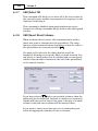
3.7
Opening an existing data file
Existing data files can be loaded into Oriana using the File|
Open 91 dialog box. Alternatively, you can choose a previously
used file from the File|Reopen 93 menu or use the drag and
drop 159 feature of Oriana. You can also load a whole set of
windows related to a data file using the desktop 4 functions.
You can keep your data files in any location you wish. The File|
Open dialog box allows you to switch to any disk or directory
accessible to your machine and will remember the last location
at which you looked for a data file. If you wish, you can have
separate directories for each project.
The Oriana program only allows a single data file (and its
related results and graph windows) to be open at any one time.
You can start a second copy of Oriana if you wish to have a
second data file open. If you already have a data file open when
Tutorial
39
you choose the File|Open command, it will be closed before
the new file is opened.
Oriana comes with a number of example data files. You can use
these to try out the program or to see the correct format for the
data files. They can be found in the SampData folder of the
Oriana program directory (usually C:\Program Files\Oriana\)
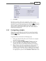
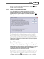
3.8
Importing data
Data can be imported into Oriana from a variety of sources,
including many spreadsheet and database formats as well as
plain text. See the section on the File|Import 94 command for
a full list of formats.
To import a file follow these steps:
1.
2.
3.
4.
Choose the File|Import command from the menu.
An Open File dialog box will be displayed. Use the Files
of type drop-down box at the bottom to choose the type of
file you wish to import. We will choose Excel for this
example.
Now select the file you wish to import. We can try
importing the ImportEx.xls file that can be found in the
Sample Data folder of the Oriana data folder (usually
found in your My Documents folder). Once the file is
selected press Open.
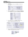
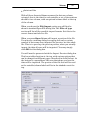
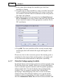
You will now be presented with an import preview dialog
box, which shows a preview of your imported data. You can
use this to check that the data are being imported
properly. If they are not then you can use the options at the
top to adjust various parameters. With this example data
set you should see six columns of data, each with a column
label (Set1, Set5, etc.) in the shaded portion at the top of
each column.
40
Oriana 4
5.
This is how we expect the data to be imported, so we can
press the OK button. The data will be imported and the
Status Window will be opened. You can use the Data|Edit
Data command to open the editor and confirm that the
data have been imported properly.
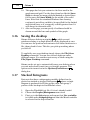
6.
This example data file has two pages of data. We can choose
to import data from the other pages. These pages are
accessed by clicking on the tabs just below the date
preview spreadsheet. To preview the second page click on
the tab named Intensive.
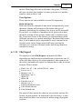
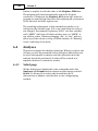
7.
This time the desired column label (Arrival) does not
appear in the shaded area. This is because the file has two
extra blank lines at the top of the sheet.
8.
To fix this problem change the Names at row option to 3,
then press Update Preview. This tells Oriana to look at
row 3 of the worksheet for the column labels. You should
now see the Arrival label in the shaded area, and the data
will now be imported properly.
Tutorial
41
Note that if you hadn’t changed the row for the column labels
Oriana would still have imported this file. However, it would
have treated the whole column as text rather than times, and
the variable type in the imported file would have been Label.
Cut and Paste
An alternative method for importing data into Oriana is to use
the Windows clipboard to transfer data directly between two
programs. To do this follow these steps:
1.
2.
3.
3.9
Create a new blank file in Oriana, as described in the File|
New 91 section. You can simply create a file with a single
column of any type.
Go to the program that you wish to copy the data from (for
example, a spreadsheet). Use the mouse to select the data
you wish to copy and choose the Edit|Copy command for
that program (clicking on the upper left corner of the sheet
headers will select all data).
Switch back to Oriana, place the cursor in the second row of
the data editor (the one with the row label Name). Then
choose Edit|Paste. The data will then be pasted into the
editor. Oriana tries to guess the correct data type for each
column, as described in the section on the Edit|Paste 103
command.
Calculating statistics
Once a data file has been created or loaded you can then
perform analyses. The Analyses 120 menu lists the various
types of analyses available. Selecting any one of these will cause
a dialog box to be displayed, giving the various options for the
analysis. When the OK button is pressed a new page will be
added to the Results window and the analysis will be
performed.
Here is an example of the steps required to calculate basic
statistics:
1.
2.
Open 38 a data file (the Wind2002.ori example data file
distributed with Oriana can be used).
Select Analyses|Stats 123 from the menu. A multi-page
dialog box, with tabs along the side, will appear. The first
page contains options to select the basic statistics you want
calculated.
42
Oriana 4
3.
4.
5.
6.
To discover what each option does you can press the large
button labeled Help to display a help page describing all
the options.
By default all circular variables in the file are included in
the analyses. If you wish to drop some of the variables go to
the Select page of the dialog. All the circular variables will
be listed on the left, with a tick mark before each. To drop
a variable just click the box containing the tick mark so
that it is cleared. We want to calculate statistics on just the
Direction variable, so clear the checkmarks on the other
variables. (Hint: You can clear all checkmarks by right
clicking on the list and choosing Deselect All from the
context menu.)
Press OK. The Results window will open, if it isn’t already
visible. A new page will be added, to which the results will
be written.
Once the analysis is finished you can look at and print the
results or export them to a file for inclusion in another
program.
Tutorial
43
Note: if you are working with frequency data (where the data
file contains a frequency table summarizing your data) then you
will need to select the Frequency option on the Select page,
rather than Raw. Then ensure that the variables selected in the
Variable and Frequency sections of the page are the desired
ones.
3.10
Selecting a subgrouping variable
By default Oriana will calculate statistics and draw graphs using
all the data from each variable. However, you may sometimes
want to calculate separate statistics and do separate graphs for
subsets of the data. You can do this by using a subgrouping
variable. This is a separate variable that contains data
specifying to which subgroup each case (or row) in the data
matrix belongs.
For example, the Wind2002.ori data file has a variable called
Month which indicates in which month each observation was
made. (See the section entitled Summarizing Data 60 to learn
how this subgrouping variable was created.) To calculate
separate statistics for each subgroup follow these steps:
1.
2.
3.
Follow steps 1-4 in the Calculating Statistics 41 section.
On the Select page of the dialog box go to the
Subgrouping box and tick the Use variable: option.
In the drop-down box below this option chose the desired
subgrouping variable (Month in this case).
44
Oriana 4
4.
Click OK. The results page will have a column of statistics
for each month.
The Subgrouping box also has options for summarizing dates.
If the variable you select as subgrouping variable is a Date one
then these options are enabled, allowing you to group the data
by Day of Week, Month of Year, Day of Year or Week of Year.
3.11
Filtering data
There are often times when you want to analyze just a subset of
your data, rather than all of it. You may want to analyze data
from just a single month, rather than the whole year, or only
those data for which an associated linear variable exceeds a
certain value. You can do this through the Filter Data 113
dialog box. You can access this in two ways: either choose the
Data|Filter Data menu item after a data file has been opened,
or click on the Filtering button on the Select page of any
analysis or graph dialog box.
To define the subset of data you wish to use you must select a
variable that contains the data you want to use to define the
subgroup, then declare the criterion to filter on. Lets say we
want to calculate statistics of the wind data in the Wind2002.
ori example data file in September alone. To do this:
1.
2.
3.
4.
5.
6.
Open 38 the Wind2002.ori data file.
Choose the Data|Filter Data 113 menu item.
Click on the Filter Data button.
Select the variable “Month” in the Variable drop-down
box.
In the Comparison Type section click the “Equal”
button.
In the Value box enter “sep” for September.
Tutorial
7.
45
Click OK.
The Status window will now be updated to show you are
filtering on the selected criterion. Now when you calculate basic
statistics, as in the Calculating Statistics tutorial 41 , only those
data recorded in September will be used. The number of
observations in the analysis will be just 700, rather than the
4495 in the full data set.
3.12
Comparing samples
Oriana has several different methods for comparing samples
within a set of data. Descriptions of each test are given in the
Analyses 63 section.
To perform these tests take the following steps:
1.
2.
3.
4.
First open the file. We will use the Termites.ori example
data file for this example.
Select the Analyses|Multisample Tests menu item.
On the first page of the dialog box select the desired
analysis. We will use the Watson-Williams F-Test here.
Most of these tests can be performed in either a pairwise
fashion (where the test is calculated for each pair of
samples) or multisample (where a single test is calculated
for all samples). Let’s first choose multisample by ticking
the appropriate option in the Calculate Tests As section.
46
Oriana 4
5.
Press OK. The test will be calculated and the results
placed in the Results window. In the first column are the
names of the samples and the numbers of observations.
The F statistic, the associated probability (p) and the two
degrees of freedom are in the following columns. A p below
your chosen alpha level (usually 0.05) means that the null
hypothesis that the samples have the same mean can be
rejected. In this case the p is 0.0104, so we can accept the
alternative hypothesis that the samples do not all have the
same mean.
6.
Let’s now investigate each pair of samples. Repeat steps 24, but this time choose the pairwise option, and press OK.
The results are reported with a line of values for each pair
of variables. The F and p values are also reported in a
matrix format at the bottom of the results page, for easier
comparisons.
Tutorial
47
We can see that most of the pairs do not have a significant
result (so the null hypothesis is not rejected), but there are
a few with p values below 0.05. For those pairs where the
null hypothesis is not rejected then Oriana also reports the
estimated population mean of the two samples.
3.13
7.
Comparing these results alongside the basic statistics
(calculated through Analyses|Stats) we can see that there
appear to be two groups of samples, some with means
around 172°-174° and some with means from 177°-181°
(note that sample Set1 has the mean reported as 0.6443°,
but since these are axial data the mean could also be
considered to be 180.6443°).
8.
We can test this by doing multisample tests of these two
groups. Again, follow steps 2-4, but this time go to the
Select page of the dialog box and untick Set1, Set6 and
Set14. The results of the F-Test on just Set5, Set8 and
Set10 gives p=0.8329, so we retain the null hypothesis
that these three samples have the same population mean,
which Oriana estimates as 173.187°. We can reverse the
state of the checkboxes so that we calculate the F-Test on
Set1, Set6 and Set14, which gives p=0.6198 and an
estimated mean of 179.491°.
Plotting graphs
Diagrams are produced through the Graphs 127 menu. We will
produce some rose diagrams and a distribution plot of the
Wind2002.ori data.
1.
2.
Open the Wind2002.ori data file.
Choose the Graphs|Histogram menu item. A dialog box
48
Oriana 4
3.
will appear.
On the first page make sure that Rose is ticked as the
graph Type.
4.
Click on the Options tab to go to that page. In Statistics
tick the Mean option, along with Confidence Intervals.
5.
On the Axes page set the Number of bars to 24 to
produce a graph with 24 bars, each 15° wide.
6.
Click on the Select tab, then untick the Month and Time
variables, so that only Direction is ticked.
Tutorial
7.
49
Press OK. The Graphs 9 window will open, if it isn’t
already visible. A new page will be added, to which the plot
will be drawn.
This diagram shows the wind direction distribution of all the
data in the file. Now let’s try creating a rose diagram for each
month.
1.
2.
3.
3.14
Again choose the Graphs|Histogram menu item. All the
options will be at the same settings used previously, so you
don’t need to follow steps 3-5 above, unless you wish to
change them.
On the Select page, in the Subgrouping box, tick the
Use variable: button then select Month from the dropdown box below it.
Press OK. Seven new graphs will be added to the Graphs
window, one for each month from June-December. These
demonstrate the variation in the wind direction through
the seasons, with it being primarily southwesterly in the
summer, but more varied in the autumn and winter.
Adjusting graph axes
Oriana has a wide variety of options that allow you to customize
the appearance of the graph. Let’s first try out some of the
options for changing the axes of the circular graph. Here is what
our graph looks like so far:
50
Oriana 4
1.
2.
3.
With the graph window topmost, showing the graph you
want to change, choose the Graphs|Edit Graph menu
item. The Histogram dialog box will appear again.
Now go to the Axes page. This has two sections, the first
for adjusting various aspects of the Angular or X Axis. This
is the one around the circumference of the circle, which
represents the angles, time of day, or other circular data. In
the graph above it is labeled 0, 90, 180, 270. The second
section is for changing the Circular or Y Axis. This is the set
of concentric rings that provide the grid representing the
frequencies in the histogram.
First lets change the Angular axis. Notice that the first
wedge in the histogram starts at 0° and goes to 15°. With
directional data, particular those based on the compass
(like our wind direction data) some people prefer to have
this first bar centered on 0°, rather than starting there. We
can do this with the Center circular bars on 0 option.
We can also tell Oriana to label the axis with compass
directions (e.g. N, S, etc.) rather than the actual angles.
Tutorial
4.
5.
3.15
51
The Label angles as compass option will do this.
By default Oriana will divide the graph into four sectors,
for N, E, S and W. We might want more gridlines than this.
We can use the Minor divisions option to specify that we
want a medium number of divisions. With compass labels
this will give us 16 divisions. We can also tick the Label
minor divisions option so that the compass directions
such as NNE and SW are used.
Finally we can reduce the number of circular gridlines in
the Circular/Y Axis section with the Number of grid
lines option. Let's set this to 3. Now press OK. Our graph
now looks like this:
Customizing graphs
1.
2.
3.
Let’s customize other aspects of the appearance of the
graph. Choose the Graphs|Edit Graph menu item. The
Histogram dialog box will appear again.
If you wish to change any of the options or even the graph
type you can do it here. We can change the current graph
into a circular histogram type by choosing the Circular type
on the Main page. Also, on the Options page we can
change the mean direction indicator into a vector, the
length of which reflects the r value for this set of data, by
selecting the R Vector option.
Go to the Fonts page by clicking on the tab at the side
labeled Fonts. Click on the button labeled Main Title. A
standard font dialog will appear. Use this to change the
52
Oriana 4
font to be used for the graph title, then press OK. Just
below this is a drop-down box labeled Title Box Style.
Use this to change the box style to Drop Shadow.
4.
5.
6.
Press OK. The graph will now be changed to a circular
histogram with an r vector, the font of the main title will
be changed to the chosen one, and a box will have appeared
around the title. These new settings will have been saved,
so all future graphs will be of this appearance, until you
change them again.
Many other options can be changed to alter the appearance.
For example, we can change the text of the title that
appears at the top of the graph. By default this is the name
of the variable. Choose the Graphs|Edit Graph menu
item again, go to the Titles page and change the Main
Title to “Wind Direction”. You could also remove the title
completely by clearing the checkbox next to the title.
Now go to the Colors page. The bars/segments of the
histograms are currently plotted in blue. You can change
this by going to the list box titled Plot Series Colors,
selecting Series 1, then changing the color with the dropdown box labeled Set Series Colors. If this plot were a
stacked or two-variable graph 54 then you could use the
other series to change the colors of other segments of the
bars.
Tutorial
7.
8.
9.
53
You can also use this page to change the background color
of various parts of the graph, and also of the lines. Click
OK to see the results.
You may wish to produce a monochrome graph, with
shaded areas rather than colored ones, for reproduction in a
print journal. You can do this by going to the Colors page
and ticking the Monochrome Graphs option. This will
disable the color selection options.
Now go to the Lines and Patterns page, where you can
use the Plot Series Patterns and Set Series Pattern
option to configure the various shading patterns, in a
similar way that you did with the colors.
54
Oriana 4
10. This page also lets you customize the lines used in the
graph axes and grid. Use the drop-down box labeled Axes
Style to change between solid and dashed or dotted lines
for the axes, and Axes Width for the width of the solid
lines. Note that the standard Windows line drawing
routines do not allow a width to be specified for the dashed
and dotted lines, so if you specify a width greater than 1 it
will always be drawn as solid.
11. Also on this page you can specify if outlines should be
drawn around the bars and symbols of the graph.
3.16
Saving the desktop
Oriana follows a desktop metaphor 4 in which several
windows relating to a single data file can be displayed at once.
You can save the position and contents of all these windows to a
file, then reload it later. This lets you pick up working where
you left off.
To explicitly save your desktop simply choose the File|Save
Desktop command. You can save several desktops under
different names. You can then restore any of them using the
File|Open Desktop command.
Oriana can be set up to automatically save your desktop when
you exit and reload it next time you run the program. This
option can be turned on in the Options|Preferences 149
dialog box.
3.17
Stacked histograms
Data sets that have a subgrouping variable defined can be
plotted as stacked or stepped histograms 85 , where a single
diagram is produced for all the groups, with each group’s
portion of the bar depicted in different colors.
1.
2.
3.
Open the Wind2002.ori file, if it isn’t already loaded.
Choose the Graphs|Histograms menu item
First go to the Select page and ensure that Use variable:
is ticked under Subgrouping and that the Month variable
is selected in the drop-down box.
Tutorial
4.
5.
3.18
55
Go to the Main page and select the type of stacked/stepped
graph you wish to produce (say, Stacked Rose).
Press OK and the graph will be produced.
Two-variable histograms
Let’s now try plotting a two-variable 86 rose diagram. This is a
rose diagram with each bar divided up into segments that
represent a frequency table of a second variable. We can use this
to show both the wind direction and wind speed from our
Wind2002.ori file.
1.
2.
3.
Open the Wind2002.ori file, if it isn’t already loaded.
Choose the Graphs|Two-Var Histograms menu item.
On the Main page of the dialog choose the Stacked Rose
option (see the section on stacked and stepped diagrams
85 for the difference between these).
4.
Now go to the Select page, where we can specify the
variable to be used as the second one. This time the
Variable box only allows a single variable to be selected.
We will select the Direction variable.
56
Oriana 4
5.
Below this is a new listbox labeled Second variable. Use
this to specify the second variable that will make up the
segments of each bar in the diagram. We will choose the
Speed variable, which represents wind speed.
6.
Let’s now look at the Options page. There is a new option
here called Exclude 0.0 values. With diagrams depicting
wind speed it is customary to not include data when the
wind speed is zero; the associated direction could be
unreliable as the wind vane could be pointing in any
direction in becalmed situations. When this option is
ticked any zero values are not included in the rose
diagram. Instead the legend box will give the percentage of
the zero values in the data set.
You can choose to have Oriana automatically divide each
wedge of the rose diagram into a certain number of
segments, using the Automatic option and the Number
of Segments setting. Each segment will represent that
proportion of the total range of the second variable. For
example, if the second variable ranges from 0 to 100,
choosing 5 segments means that the first one will
represent the number of observations between 0 and 20,
the second from 20-40, and so on.
7.
Tutorial
8.
57
If you prefer you can set the boundaries between each
segment manually, using the Manual option above. This
lets you enter the exact boundaries for each segment. So, in
the above example of a variable ranging from 0-100, if you
enter a 15 in this option as the first boundary and a 30 as
the second then all values from 0-15 will be in the first
segment, all values greater than 15 and up to 30 are in the
second segments, and so on.
To build up your list of boundaries tick the Manual
option, then enter the first boundary into the Boundary
box and click the Add button. This will add the boundary
to the box below. Continue doing this for all boundaries. If
you need to remove a boundary you can select it in the list
and click the Remove button.
If your second variable consists of discrete values (e.g. just
the numbers 1, 2, 3 and 4) and you want a separate
segment for each you can use the Segment for each
unique value option.
3.19
Circular-linear plots
The process of producing circular-linear plots 87 is similar to
that described in the previous section for two-variable
histograms. However, in this case the value of the second
variable is represented by the length of the arrows or bars, or by
the placement of the points on the graph, each of which
represents a single case (or row of the data matrix). We can
58
Oriana 4
demonstrate this graph type by again using the Wind2002.ori
file.
1.
2.
3.
4.
5.
6.
7.
8.
3.20
Open the Wind2002.ori file, if it isn’t already loaded.
Choose the Graphs|Circular-linear Plot menu item
On the Select page ensure that subgrouping is by Month,
as done in step 3 of the Stacked Histogram 54 tutorial.
Also ensure that the primary and second variables are set
to Direction and Speed respectively, as in steps 3-4 of the
Two-variable Histogram 55 tutorial.
On the Main page of the dialog you can choose to have the
data represented as a scatterplot, or with arrows, bars or
wedges.
You can use the Symbol size option on the Symbols page
to determine the size of the scatterplot symbols, and the
Arrowhead size option on the same page to adjust the
arrowheads. If the Variable arrowhead size option is
ticked then arrowheads closer to the center of the graph
will be made smaller. Since shorter arrows have their
heads packed more closely together this helps make the
individual arrowheads more easily visible.
If instead you are using bars the width of the bar is
controlled by the Bar width option on the Axes page. By
default this is set to 1 degree wide, but you may wish to
make them a bit wider.
By default, using Month as the subgrouping variable means
that a separate graph is created for each month. If you
instead wish to have all data on the same graph, with
different colors or symbols representing the different
subgroups, you can tick the Subgroups on single plot
option on the Main page. For scatterplots you can choose
to use different colors, symbols, or both with the
Represent subgroups with option on the Symbols
page.
Printing graphs and results
The contents of most window types can be printed using the
File|Print command. You must first make sure that the
window you want to print is the currently active window. In the
Print Range section you can select to have just the current
graph printed or all graphs.
You can specify which printer to use and change other options
with the File|Printer setup 100 command. The size of the
Tutorial
59
margins on the printed page can be changed with the File|
Page setup 101 command.
3.21
Saving graphs and results to file
The contents of the graph and results windows can be saved to a
file using the File|Export 97 command. You must first make
sure that the window you want to save is the currently active
window and that the page with the graph or results you want to
save is visible. If you tick the Export all pages option on the
dialog all graphs or result pages will be exported. For graphs
each files is exported to a separate file. The file names will have
sequential numbers appended to your chosen file name to
distinguish them. All result pages will be exported to a single
file.
Different types of windows have their contents saved in
different formats; some may have a choice of formats for saving.
See the descriptions of the window types 5 for more details.
3.22
Changing variable type
You may occasionally find that you need to change the type of a
variable. Most often this is when you are creating a new data file
in expert mode. In this mode a blank data editor window is
displayed with all the variables set to be of the type Angle. You
will then need to change the variable types to suit your purpose.
You may also decide later, after entering some data, that
another data type might be more appropriate.
The simplest way is to use the drop-down boxes at the top of
each column. Just click on the small downward pointing arrow
and select the new type from the list.
60
Oriana 4
You can also use the Data|Change Variable Type 107 menu
item. This will display a dialog box with all possible data types.
It will also let you change the grouping state 26 of the circular
data.
3.23
Summarizing data
You may sometimes wish to summarize a variable to allow for
particular types of analyses. For example, if you have recorded
the exact date of an event you may wish to summarize these by
month, so that you can look at trends throughout the year.
You can do this by creating a new variable from the original
date one. This is done with the Data|Change Variable Type
command.
1.
Place the cursor in the column of the desired date variable
in the data editor and choose the Data|Change Variable
Type menu item.
Tutorial
2.
3.
4.
61
In the Basic Type section choose the desired type of the
new variable (Month of year in this case).
Ensure that the Create new variable option is ticked.
Click OK. A new variable will be inserted next to the date
variable, containing the month of year corresponding to
each date.
Analyses
4
63
Analyses
There are several types of analyses that Oriana can perform.
Some procedures will give you basic statistics on each sample
whereas others will allow you to compare samples to test
whether they differ significantly.
In the descriptions that follow the basic concept behind the
analyses and Oriana’s particular implementation is given. For
details and a greater understanding of the analyses you should
look to some of the circular statistics literature. The references
158 section of this document lists many references, and in the
following text page references are given to some of the
textbooks that describe the analyses.
4.1
Statistics
Oriana calculates a variety of special circular statistics on each
sample. These are mainly descriptive statistics, similar to those
provided by other general statistics packages, but they are
special versions designed for circular data. There are also a
number of one sample tests of probability. The statistics
included in Oriana are described briefly in the next two
sections. See the section on the Analyses|Stats 123 command
for details on how to run these analyses.
4.1.1
Basic Statistics
Many of the basic statistical parameters are based on the
concept of the mean vector. A group of observations (or
individual vectors) have a mean vector that can be calculated by
combining each of the individual vectors (the calculations are
explained in most books 158 about circular statistics).
64
Oriana 4
The mean vector will have two properties; its direction (the
mean angle, µ) and its length (often referred to using the letter
r). The length will range from 0 to 1; a larger r value indicates
that the observations are clustered more closely around the
mean than a smaller one.
The concentration ( is a parameter specific to the von Mises
distribution and measures the departure of the distribution
from a perfect circle (or a uniform distribution). It is related to
the length of the mean vector. The value reported by Oriana is
the maximum likelihood estimate of the population
concentration, calculated using the formula in Fisher (1993,
p.88) and Mardia & Jupp (2000, p.85-6).
The circular variance and circular standard deviation are
equivalent to their linear counterparts, but are calculated in a
much different way. Variance is calculated from the length of
the mean vector through the simple formula V = 1 - r;
standard deviation is then calculated by S = (-2 ln(r))½. The
result S, which is in radians, may then be converted to degrees
by multiplying by 180/
Analyses
65
The standard error of the mean is also calculated based on the
length of the mean vector (r) and the concentration, and is
calculated using formula 4.42 in Fisher (1993). It assumes that
your data adhere to the von Mises distribution. The 95% and
99% confidence intervals are then derived from the standard
error as would be done for the normal distribution (i.e.
multiplying by 1.9604 or 2.5762). When the standard error is
calculated a check is made of the concentration for the sample
as well as the sample size. The standard error can be unreliable
if the combination of these is low. If this occurs a warning will
be printed.
The circular median direction can be difficult to calculate, due
to the problem of choosing an appropriate axis on the circular
scale, which wraps around. In Oriana the median is calculated
by minimizing the function:
d( )
1
n
n
i
i 1
This is from equation 2.32 of Fisher (1993; note that earlier
hardback printings of that book accidentally leave out part of
this equation) and finds the absolute difference between the
test median direction and all the data values i. This
minimization process can take a long time for large data sets, so
it is advised that you leave the Median option on the
Analyses|Stats 123 dialog box unticked unless you need the
median.
When circular data are grouped 26 a bias can occur in the
calculation of r. This can be corrected by multiplying r by a
correction term (Zar, 1999, p.601; Mardia & Jupp, 200, p.23),
calculated as c = (cw/2) / (sin(cw/2), where cw is the width of
each class of the grouped data, in radians. For classes less than
30° in width this correction is negligible, so is not applied.
If the variable type 13 being analyzed is Axial then the data are
doubled (modulo 360) before being analyzed. The resulting
mean direction is then back converted to be within 0°-180°. The
other mean-related statistics are also back-converted.
Weighted Statistics
If your data consist of vectors (where both the angle and the
length have been recorded) and you have defined vector pairs
66
Oriana 4
using the Data|Define vector pair 114 command, then a
weighted mean vector will also be displayed. This is the angular
mean, but weighted by the lengths of the vectors. The length of
this mean vector is also given, first in the native units of the
weighting variable, then scaled 0-1 like the unweighted r. This
is followed by the X and Y components (sin and cosine) of the
standard deviation ellipse. This is an ellipse depicting the
standard deviation that can be drawn around the weighted
mean centroid on circular-linear graphs 142 . Basic statistics
about the weighting variable will also be displayed.
Also displayed are two hypothesis tests. Hotelling's test
(Batschelet, 1981, p. 144) tests whether the centroid of the end
points of the weighted vectors differs from the origin effectively, whether the weighted angles have a significant
mean direction. The null hypothesis is that there is no mean
direction. A probability less than your chosen significance level
(usually 0.05) indicates that there is a common mean direction
to the population. It is assumed that the data are not grouped,
and that they conform to the bivariate normal distribution.
Note that the test is particularly sensitive to departures due to
skewness.
Moore's Modified Rayleigh Test (Zar, 1999, p.639-641) is a
nonparametric analogue of the Rayleigh test for testing if angles
are uniformly distributed around the circle. The null hypothesis
is that the data are uniformly distributed. If the p value is less
than the chosen significance level (usually 0.05) then the
alternative hypothesis that the data are not uniformly
distributed is accepted.
Analyses
4.1.2
67
One Sample Tests
Rayleigh’s Uniformity Test (Fisher, 1993, p. 70; Zar, 1998,
p.616; Mardia & Jupp, 2000, p.94) calculates the probability of
the null hypothesis that the data are distributed in a uniform
manner. The Z value is calculated simply as Z = nr2, where n is
the number of observations and r is the length of the mean
vector. A longer mean vector (and the resulting larger value of
Z) means greater concentration of the data around the mean,
and thus less likelihood of the data being uniformly distributed.
The calculation of the probability follows Fisher’s equations
4.17 and 4.18. A probability less than your chosen significance
level (usually 0.05) indicates that the data are not distributed
uniformly and that they show evidence of a preferred direction;
the preferred mean direction is unspecified, as opposed to the
V-test discussed below.
In the above example the Rayleigh Z value is very high and the
probability vanishingly small, so we reject the probability that
the data are uniformly distributed.
Note that in the Results window a ‘< 1E-12’ (which stands for
68
Oriana 4
< 1x10 - 1 2 ) means that the actual value is indistinguishable
from zero at the maximum accuracy of the computer (15-16
significant digits). Values that are somewhat larger, but still
smaller than the number of decimal places set in Options|
Format 149 , are given in scientific notation (e.g. 0.0000025, or
2.5x10 - 6 , is displayed as 2.5E-6).
Rao’s Spacing Test (Mardia & Jupp, 200, p. 108; Batschelet,
1981, p.66) also takes as its null hypothesis that the data are
uniformly distributed. This is tested by looking to see if the
spacing between adjacent points is roughly equal around the
circle (using the equations on the above cited pages). For
uniform distribution the spacing between points should be
roughly 360°/n. If the actual spacings deviate too much from
this value then the likelihood that the data are uniformly
distributed is reduced.
This test can be more powerful than Rayleigh’s test. For
example, the data in the graph below seem to be non-uniform,
appearing to be bimodal. However, the length of the mean
vector is very small (note the short mean arrow on the graph)
and Rayleigh’s test gives a non-significant result, with a
probability of 0.811. However, Rao’s spacing test gives a
probability less than 0.01, and the null hypothesis of uniformity
can be rejected.
Watson’s U² Test (Fisher, 1993, p. 84; Mardia & Jupp, 2000,
p.104; Zar, 1999, p.657; Batschelet, 1981, p.79) performs a
goodness-of-fit test against a specified distribution, either
uniform or von Mises. It does this by calculating the mean
square deviation for the fitted distribution. If the deviation is
too high (resulting in a high U² and a low probability) then the
null hypothesis that the data fit the chosen distribution is
rejected. When the uniform distribution is selected the
Analyses
69
modified statistic, as shown in Fisher’s (1993) formula 4.36 or
Mardia & Jupp’s (2000) formula 6.3.36 is used.
This test cannot be calculated on grouped
used for sample sizes less than 10.
26
data, nor can it be
Kuiper’s Test (Fisher, 1993, p.66; Mardia & Jupp, 2000, p.99;
Batschelet, 1981, p.76) takes the alternative approach of
directly comparing the distribution of the data to the desired
distribution, either uniform or von Mises. It can be viewed
graphically by referring to the distribution plots 88 produced
by Oriana. The Kuiper’s V statistic is based on the largest
vertical deviations above and below the diagonal line
(representing the desired distribution). Too great a deviation,
giving a high V and low probability, leads to rejection of the null
hypothesis that the data fit the distribution.
The formula used in Oriana incorporates the correction factor
shown in Fisher’s (1993) equation 4.12 and Mardia & Jupp’s
(2000) 6.3.30. As with Watson’s U², this cannot be calculated
on grouped 26 data.
For grouped data the Chi-squared Test (Batschelet, 1981,
p.72; Zar, 1999, p.656) is instead calculated. This simply
performs a standard chi-squared test based on the expected
number of observations in each class given a uniform
distribution. A probability below the chosen alpha level (usually
0.05) leads to the rejection of the null hypothesis that the data
are distributed uniformly. The sample size must be sufficient so
that the expected frequencies in each class are 2 or greater.
If you wish to perform the chi-squared test on data that are not
grouped you will have to first declare them as grouped and set
the class width, using the Data|Change Variable Type 107 dialog
box.
The V-Test (Fisher, 1993, p.69; Mardia & Jupp, 2000, p.98;
Batschelet, 1981, p.58; Zar, 1999, p. 618) is a variant of the
Rayleigh test, but instead of testing the null hypothesis of
uniformity against an unspecified alternative, the V-test tests
against an alternative hypothesis that the distribution is a nonuniform one with a specified mean direction. The specified
mean direction is a hypothetical one chosen in advance (for
example, the expected vanishing direction of released homing
pigeons).
70
Oriana 4
Note that Zar (1999) calculates V from R, the total length of the
resultant vector of the data, rather than from r, the length of
the mean vector, which is what most other authors (and Oriana)
use. However, Zar’s formula for u corrects for this; thus u and p
will be the same for all methods.
4.1.3
Second Order Statistics
If two or more circular variables are present in the file, or if a
subgrouping variable is being used to analyze sets of data, then
second order statistics are also calculated. These are statistics
that focus on further analyses of the basic statistics for each
variable.
The first statistics are the calculation of the grand mean
vector, or the mean of means. This is calculated in a similar
way to the mean of each variable,with the means for each
variable being used as the data rather than the original angles.
Also, each mean is weighted by its r value (the length of the
mean vector). The result is a grand mean angle and its resulting
length r. Also provided are the 95% and 99% confidence
limits, calculated using the method of Batschelet (1981), also
described in Zar (1998, p. 611) . Note that, unlike the
confidence intervals for the sample means, these are not
necessarily symmetric around the grand mean. Also, the
confidence intervals often cannot be calculated when the
number of means are small (e.g. less than 4-5).
Two hypothesis tests are also calculated. Hotelling's one
sample test (Zar, 1998, p. 638; Batschelet, 1981, p. 144) tests
whether the whole population has a significant mean direction.
The null hypothesis is that there is no mean direction. A
Analyses
71
probability less than your chosen significance level (usually
0.05) indicates that there is a common mean direction to the
population. It is assumed that the data are not grouped, and
that they conform to the bivariate normal distribution. Note
that the test is particularly sensitive to departures due to
skewness.
A nonparametric test is also available. Moore's modified
Rayleigh test (Zar, 1998, p. 641) is an analogue of the Raleigh
test that is based on weighting the mean angles with the rank
order of the r values of each. The null hypothesis is that the
means of the population are uniformly distributed around the
circle. A significant probability indicates that the data are not
distributed uniformly and that they show evidence of a
preferred direction.
4.2
Multisample Test
The multisample tests in Oriana allow you to compare two or
more sets of data to determine if their distributions differ. Most
tests can be performed either as pairwise, where each pair of
samples are compared, or as multisample, where all samples are
compared at once. The tests included in Oriana are described
briefly in the next sections. See the section on the Analyses|
Multisample Tests 124 command for details on how to run
these analyses.
4.2.1
Watson-Williams F-Test
Watson-Williams F-test (Fisher, 1993, p.126; Mardia & Jupp,
2000, p.129; Batschelet, 1981, p.95; Zar, 1999, p. 625)
compares two or more samples to determine if their mean
angles differ significantly. The test can be performed in a
pairwise fashion, so that the selected samples are compared
with each other, a pair at a time, or an overall test can be
calculated for all samples.
The F-test basically proceeds by comparing the lengths of the
mean vectors for each sample with that for the pooled data of
the two or more samples. The resulting F statistic is the same
as Fisher’s variance ratio statistic which is commonly used in
linear statistics, including analysis of variance. The p value
printed for each test is the probability associated with the null
hypothesis that the two mean angles are equal. If this
probability is less than your chosen significance level (usually
0.05) then the null hypothesis can be rejected in favor of the
72
Oriana 4
hypothesis that the means are different. If the null hypothesis
is not rejected (i.e. the probability is greater than 0.05) then
Oriana will report the overall mean for all samples in the test,
which can be used as an estimate of the overall population
mean.
This test assumes that the two samples are independent and
drawn at random from a population with a von Mises
distribution. It also assumes that the concentrations of the two
samples are similar and that they are sufficiently large (>2). If
the concentration is too low, a warning is printed. Finally the
data may not be grouped 26 .
The formula for the F-test can incorporate a correction factor,
based on the concentration, to correct for bias. Some authors
only use this when concentrations are low, whereas others use it
for all calculations; Oriana ver. 2 takes the latter approach
(Oriana ver. 1 only used it for estimated concentrations between
1 and 2).
4.2.2
Chi-Squared Test
Oriana can perform pairwise or multisample Chi-squared
Tests (Batschelet, 1981, p.109) on the samples. This test
determines whether the samples differ significantly from each
other in some unspecified way.
The test is the basic chi-squared test as used for a variety of
purposes. The data must first be grouped into classes. For data
that are already grouped 26 their specified class width is used;
otherwise the class width can be set through the option on the
Options page of the Analyses|Multisample Tests 124 dialog
box. A contingency table is then constructed and the expected
frequencies determined (based on the row and column totals).
The Chi-Squared statistic is then calculated based on the
differences between the observed frequencies of the samples.
The p value printed for each test is the probability associated
with the null hypothesis that the samples are drawn from the
same population. If this probability is less than your chosen
significance level (usually 0.05) then the null hypothesis can be
rejected in favor of the hypothesis that the samples are from
different populations that differ in some way. The difference
may be in the distribution, mean direction, or other parameter;
further investigation will be needed to determine what the
Analyses
73
difference is between the two samples.
The Chi-squared test assumes that most or all the expected
frequencies used in the calculation will be greater than 5. This
is checked during calculations and a warning is printed if more
than 20% of the classes have expected frequencies less than 5. If
this occurs you can try using large class widths so that more
observations are in each class. You can also use the Drop
Classes with 0 Observations option on the Options page of
the analysis dialog box. This will ignore any classes that do not
have any observations. This is particularly useful if your
observations are clustered fairly closely around the mean, with
the result that a large portion of the circle will not have any
data.
4.2.3
Mardia-Watson-Wheeler Test
The Mardia-Watson-Wheeler Test (Fisher, 1993, p.122;
Mardia & Jupp, 2000, p.147; Batschelet, 1981, p.101; Zar,
1999, p. 633), also called the Uniform Scores Test, is a nonparametric test for determining whether two or more
distributions are identical. The basic idea is that the samples
are pooled together, sorted into increasing angles, and are then
evenly distributed around the circle by calculating a uniform
score (or circular rank). If the distributions of the samples are
identical then the new uniform scores for the samples should be
evenly interspersed around the circle, and their resultant vector
lengths R should be short and similar. Any significant
difference between the Rs will lead to a large W test statistic
and rejection of the null hypothesis of identical distributions.
It is important for this test that any ties between samples (e.g.
identical angles, such as 135°, in two or more samples) are
broken. Oriana does this by randomly assigning different ranks
during the ranking procedure. The actual ranks assigned will be
the same for subsequent runs of the test, so long as the order of
the original data remains the same. However, if you re-sort the
data and run this test again you may get a different result for W,
because the randomly assigned ranks will differ. If this is likely
to cause problems you may wish to break any ranks manually
before running the test. You can do this by replacing the
identical values with two slightly different values (e.g. replace
two 135° observations with 134.999° in one sample and 135° in
the other). You must remember, though, that this may cause
unwanted effects in other statistical procedures.
74
Oriana 4
This test cannot be performed on grouped
4.2.4
26
data.
Watson's U2 Test
Watson’s U² Test (Mardia & Jupp, 2000, p.150; Batschelet,
1981, p.114; Zar, 1999, p. 630) is a two-sample analogue of the
single sample Watson’s U² 68 test; instead of comparing a set
of data to a theoretical distribution two sets of data are
compared using mean square deviations. The null hypothesis is
that the two samples have the same distribution. A significant p
value leads to the rejection of this hypothesis and the
acceptance of the alternative hypothesis that the samples are
from populations that differ in some way. The difference may be
in the distribution, mean direction, or other parameter; further
investigation will be needed to determine what the difference is
between the two samples.
As with the single sample test, the two-sample Watson’s test
cannot be performed on grouped 26 data.
4.2.5
Hotellings Paired Test
Hotelling's Paired Test (Zar,1999, p. 645) compares two
samples of paired data using Hotelling's procedure. This tests
whether the paired observations differ between the two
samples. The null hypothesis is that there is no difference
between the two samples. A probability less than your chosen
significance level (usually 0.05) indicates that the pairs differ
between the samples. It is assumed that the data are not
grouped, and that they conform to the bivariate normal
distribution. Note that the test is particularly sensitive to
departures due to skewness.
Note that this test is for use with paired sample experimental
designs and that it is assumed that each row in the matrix is for
an individual case (for example, each row contains data for an
individual organism before and after treatment or in two
different situations). If one sample has more cases than the
other all the extra cases will be treated as missing data and will
be ignored.
4.2.6
Moore's Paired Test
Moore's Paired Test (Zar,1999, p. 647) is a nonparametric
alternative to Hotelling's Paired Test. This also tests whether
Analyses
75
the paired observations differ between the two samples, using
Moore's modified Rayleigh test. The null hypothesis is that
there is no difference between the two samples. A probability
less than your chosen significance level (usually 0.05) indicates
that the pairs differ between the samples.
As with Hotelling's, this test is for use with paired sample
experimental designs and that it is assumed that each row in
the matrix is for an individual case.
4.3
Correlations
Oriana provides two different correlation procedures for
comparing variables, one between two circular variables and one
between a circular and a linear one. These correlations assume
that the data are entered in a pairwise fashion; that is, each row
in the data matrix contains data related to the same
observation or sample. For example, a data set may contain two
variables, one the direction of travel of an insect and the other
the direction to a light source. Each row would represent the
observation of these two directions at a single point in time.
These correlations are described briefly in the next sections. See
the section on the Analyses|Correlations 125 command for
details on how to run these analyses.
4.3.1
Circular-circular correlation
The circular-circular correlation coefficient (Fisher, 1993,
p.151; Mardia & Jupp, 2000, p.250; Zar, 1999, p. 649)
calculates the correlation between two circular variables. This
uses the Fisher & Lee (1983) method, which is analogous to the
Pearson product-moment correlation commonly used for linear
data. As with Pearson’s this coefficient ranges from -1 to +1,
with the former indicating a perfect negative correlation, the
later a perfect positive correlation, and 0 indicating no
correlation.
The formula used for the calculation is the alternative form
given in Fisher’s (1993) equation 6.36. The significance of the
correlation is tested by using the jackknife method described in
Zar (1999, p.649-650). With this the correlation is calculated
multiple times, each time with one pair of data being dropped.
The confidence limits of the series of calculated coefficients is
then calculated; if 0 does not fall within the limits then the null
hypothesis that the correlation is 0 is rejected, and the
76
Oriana 4
alternative that the correlation is significantly different than 0
is accepted.
Note that the jackknife calculation can take a long time for
large data sets, so this is an option in the Analyses|
Correlations 125 dialog box.
4.3.2
Circular-linear correlation
The circular-linear correlation coefficient (Fisher, 1993, p.145;
Mardia & Jupp, 2000, p.245; Zar, 1999, p. 651) calculates the
correlation between a circular variable and a linear one.
Examples of data where one might want to calculate this type of
correlation could include wind direction and ozone level, or
direction of travel of an animal along with the distance traveled.
This correlation coefficient ranges from 0 to 1, so there is no
negative correlation. The calculation of the significance of the
correlation follows Mardia & Jupp (2000) in using their
approximation of the F distribution in equation 11.2.2.
4.4
Second Order Statistics
The Basic Statistics analysis in Oriana will provide second order
stats (e.g. the grand mean) if there are more than one variable of
raw data. It will do this by calculating the means and mean
vector length for each variable, then calculating the second
order statistics.
However, you may already have your data in the form of means
and mean vector lengths, so may wish to calculate the second
order statistics directly on those means. The analyses in
Oriana's Second Order Statistics command will do this. To run
these analyses your data file needs to have pairs of variables,
one circular and one linear, which contain the polar coordinates
of the mean vectors - the means and their associated lengths.
You can have a number of pairs of variables, but Oriana will
always assume that the first linear variable is associated with
the first circular one, the second linear with the second circular,
etc.
4.4.1
Basic Second Order Statistics
The first section of the Second Order Statistics output is similar
to that produced when calculating the basic statistics 70 on raw
data. The grand mean and its length, the confidence intervals,
Analyses
77
and Hotelling's and Moore's tests are output. If the data file
contains more than one pair of variables containing the means
and lengths then a column of results is produced for each pair.
4.4.2
Two Sample Second Order Statistics
If there are two or more pairs of mean and mean vector length
variables in the data file then two sample second order tests are
also calculated. First in the table of results are the names of the
two sets of means/lengths that are being compared, along with
the number of means in each sample. This is followed by a
number of test results.
78
Oriana 4
Hotelling's two sample test (Zar, 1999, p.641-642;
Batschelet, 1981, p. 150-154) compares the grand means of two
populations. The null hypothesis is that the means of the two
populations are equal. A probability less than the chosen
significance level (usually 0.05) indicates that the two means
differ. As with other variations on the Hotelling test, this
assumes that the data are not grouped, and that the data are
from a bivariate normal distribution with similar variances.
However, this two-sample test is somewhat more robust to
departures from normality than the one sample and paired
tests.
A nonparametric alternative to the above is Mardia's two
sample test (Zar, 1999, p.643-645; Batschelet, 1981, p. 154156). With this test the differences between the individual
means and the grand mean for both samples is further analyzed
using one of the circular two sample tests. In Oriana Watson's
U² is used for the analysis. The null hypothesis is that the two
samples come from the same population. The alternative
hypothesis is that the populations that differ in some way (in
the distribution, mean direction, or other parameter). This test
cannot be used on grouped data.
These tests are followed by Hotelling's paired two sample
test 74 , and Moore's nonparametric alternative 74 . These
are identical to the paired tests described above in the
Multisample Test section, except that they are calculated on
samples of means rather than raw data. As with those it is
assumed that the data are paired (e.g. each row in the data
matrix contains the means for the same population, but
measured before and after some treatment or change in
circumstances).
Graphs
5
79
Graphs
Oriana allows you to plot your data in a number of ways. There
are a variety of circular graphs as well as traditional linear
histograms and scatterplots. There is also a graph that plots
your data against an expected uniform distribution to allow you
to assess whether your data depart from uniformity, and a
similar graph that compares two sample distributions.
For more details about how to actually produce these charts, see
the tutorial section on graphing your data. 47
5.1
Rose Diagrams
This is one of the most commonly used types of graphs for
circular data. It is basically a histogram that has been wrapped
around a circle. Each section of the histogram, which in this case
is wedge-shaped, depicts the number of observations falling
within that portion of the range. In the graphs shown below
each wedge represents 10° of the total circular range and the
length of each wedge (the radius from the center) represents the
number of observations falling within that range. The data are
tabulated so that the lower end of the range is included in the
bar, but not the upper end (e.g. the first bar includes values
ranging from 0° to just less than 10°, the second one ranges from
10° to just less than 20°, etc.).
Note that the above graph has a black line running from the
center of the diagram to the outer edge, at approximately
17:00. This is the mean angle of the data. The arcs extending to
either side represent the confidence limits of the mean. They
can be either the 95% or 99% confidence limits, depending on
80
Oriana 4
the setting in the Graphs|Histograms 133 dialog box. Note
that sometimes the confidence limits can be unreliable when
the combination of the sample size and the concentration is low.
In these cases the confidence limit arc can be displayed in a
different color. By default this is red rather than black, but the
color can be changed with the Inacc. Stats option on the
Colors page of the dialog box.
As an alternative, the mean can also be depicted as an arrow,
the length of which represents the value of r (which is described
in the section on Basic Statistics 63 ).
The above type of graph can be misleading, because our visual
perception takes the whole area of a wedge into account when
comparing them, rather than just its length. A wedge that is one
third the radius of another actually appears far less important,
since the area of the smaller wedge is only one ninth the area of
the larger one. To avoid this problem, the wedges can be drawn
so that the frequency is represented by the area of the wedge.
The following graph uses the same data as the one above, but
the area option has been selected.
Note that the scale is now a squared scale rather than a linear
one.
With compass direction data the wedges of the diagram are
shifted slightly so that they are centered on the compass
direction. For example, in the diagram below the wedge for
North directions is centered on the vertical axis (0° or N), rather
than having its left edge starting at that point. This type of
placement can also be optionally specified for graphs of angular
or time data, through the Center circular bars on 0 option
Graphs
81
on the Axes page of the Graphs|Histograms 133 dialog box.
5.2
Circular Histograms
These graphs are similar to the rose diagram, but they are made
up of parallel-sided bars that show the number of observations
within each class range. The actual width of the bars (= the
width of the class range) can be set when the graph is drawn.
The graph below has a bar width of 10 degrees.
5.3
Raw Data Plots
These circular diagrams plot individual symbols for each datum
in the sample. This allows you to assess the sample size at a
glance as well as seeing the distribution of the data.
Here is an example of one traditional way of presenting the raw
data, with the points stacked from the outer rim of the circle
82
Oriana 4
towards the middle:
You can also have the points stacked on the outer rim, pointing
outwards:
Finally you can have the points stacked from the middle
pointing outwards:
Graphs
83
Note: For samples with very large numbers of observations,
each symbol may represent multiple observations; a note will
be placed on the graph if this occurs. If you want to reduce it to
one symbol per observation you can try taking one or more of
the following steps:
Reduce the size of the symbols on the Symbols page of the
graph dialog box
Switch to using a different type of raw plot (e.g. from points
arranged margin inwards to margin outwards)
Adjust the Basal Circle option on the Axes page to make it
smaller (for margin outwards and center outwards graphs
only).
Increase the overall size of the graph by making the graph
window and/or the whole Oriana window bigger.
5.4
Arrow Graphs
This graph is similar to a circular histogram 81 , but instead of
parallel-sided bars it has arrows indicating the frequencies for
each class.
84
5.5
Oriana 4
Linear Histograms
Circular data can also be plotted on linear histograms. In this
case the mean vector and the confidence limits are show as
vertical lines.
If you wish to emphasize the cyclicity of the data you can choose
to have the X axis doubled, so two complete cycles of the data
are plotted:
Graphs
85
You can also choose to have just half the scale depicted. This is
useful if you are working with axial data all in the 0-180° range.
5.6
Stacked and Stepped Histograms
If your current data file has a grouping variable defined then
normally separate graphs will be produced for each group.
However, you can also produce a single graph that has
differently colored segments for each group, showing the
relative proportions of each.
The above graph was produced by first ensuring that a grouping
variable was selected (DOW in this case) and then choosing the
Stacked Rose option on the Graphs|Histograms 133 dialog
box. Choosing Stacked Circular will give a similar graph, but
with parallel-sided bars, and Stacked Linear will give a linear
histogram 84 with stacked segments.
By default a single mean will be displayed for the whole data
set. However, you can optionally specify that the mean for each
86
Oriana 4
subgroup is displayed by selecting the Subgroup means
option on the Options page of the Graphs|Histograms 133
dialog box.
The Stepped Circular option will produce a circular
histogram with each segment being somewhat thicker than the
previous one. This type of graph is commonly used for
meteorological wind roses.
5.7
Two-variable Histograms
Segmented histograms like the Stacked and Stepped 85 ones
can also be produced from two separate variables, where one is
circular and the other is a set of associated data. Examples
would be wind direction and speed, or the direction and
distance of travel of an animal. This graph is formed by dividing
up the second variable into frequency classes and using those as
the segments of the graph.
In the above graph zero values for the wind speed are left out of
Graphs
87
the graph, as is common in meteorological studies, where the
direction measured during becalmed periods could be
misleading. This is an option on the Graphs|Two-Var
Histograms 138 dialog box. Also on this dialog box is the
Subgroup means option, which specifies that separate means
are displayed for each class of the second variable.
5.8
Circular-linear Plot
This graph type, like the two-variable histogram, also plots two
variables, one circular and one linear. However in this case the
second variable is depicted not as frequencies in segments of the
histogram, but as individual points. Each observation, or row in
the data matrix, is depicted as a point, arrow, bar or wedge.
The first type, the scatterplot, has each observation represented
by a point. The position around the circular axis represents the
circular variable, while the position on the concentric grid
represents the linear value. Here is an example:
The vector type of circular-linear plot is superficially like the
Arrow Histogram 83 , but in this case each arrow corresponds to
a single observation. The direction the arrow is pointing is
taken from the selected circular variable, while the length of
the arrow is determined by the chosen second variable. So you
could, for example, use this graph to plot the direction and
distance traveled for each animal observed, or the orientation
and length of individual toolmarks in sedimentary rocks.
88
Oriana 4
Instead of arrows, you can also choose to have the linear variable
represented by bars or wedges.
5.9
Distribution Plots
Distribution plots allow you to assess the departure of your data
from a certain distribution, such as uniformity. Each datum is
plotted against the value expected for that datum given the
desired distribution. The points on the plot should lie along a
45° angle; the diagram has a reference line at this angle.
Departures from the distribution can be seen as departures
from this line. The following graph compares arrival time
against a uniform distribution; it is clear that there are
departures from uniformity.
Since the data are circular, and the starting point of the plot is
arbitrary you could have important patterns becoming less
noticeable if they occur split over the wrapped around part of
the plot (i.e. going off the graph at the upper right and wrapping
around back to the lower left). This can be alleviated by
extending the axes and repeating 20% of the points at either
end. The following graph is the extended version of the one
Graphs
89
above.
The next graph compares the data to the von Mises distribution.
Here you can see a close correlation, suggesting that the data
follow the von Mises distribution.
5.10
Two-sample Graphs
The Graphs|Two-sample 145 command produces scatterplots
and two sample Q-Q-plots. With the Scatterplots option you
can plot any two variables against each other. This is useful to
give a graphical representation that can be used in interpreting
the results of a correlation 75 analysis. Options on the dialog
box allow you to reverse the X and Y axes, and also to specify
whether the whole 0-360 range for circular data is plotted, or
only that part of the scale that actually has data.
90
Oriana 4
Q-Q plots are ones that let you compare the distribution of two
samples, much like the distribution plots 88 compare a single
sample against a theoretical distribution. They are produced by
first centering the data on their medians (so that any
differences in the medians do not affect the graphs) and then
sorting them into ascending order. These are then plotted
against each other. If the two samples have different numbers of
observations the number of points plotted is the lower of the
two. Observations to be plotted from the larger of the samples
are chosen to be evenly distributed throughout the range.
If the two distributions are similar then the points will lie close
to the 45° angle reference line. In the following graph the points
make a distinct departure from the reference line, and thus it
appears that the two distributions are different. This is
confirmed by significance levels far below 0.05 for the MardiaWatson-Wheeler 73 and the Watson’s U² 74 test.
Menus
6
91
Menus
This section describes the menu structure of Oriana.
6.1
File
The File menu contains the commands for opening and saving
data and desktop files, as well as the printer related functions.
All of the save and print functions act on the currently active
window.
6.1.1
File|New
This option allows you to set up a new data file. You can specify
the initial size of the data file and the types of data. 12
When you choose the File|New command, one of two New Data
dialog boxes will be displayed, depending on which you used
last. By default the New File Wizard is displayed. This takes
you step by step through declaring what type of data you are
going to enter and how many columns there are, and giving
labels to each variable and the whole file. At the end, after
pressing the Finish button the status window will be displayed
and an empty spreadsheet will be opened, ready for you to enter
data.
You can also switch to Expert Mode by pressing the appropriate
button. In this mode you simply enter the number of columns
you wish to have in your file and press OK. Once the data editor
is displayed you can then declare the type of each variable with
the Data|Change Variable Type 107 option, or by using the
drop-down boxes in the first row of each column.
6.1.2
File|Open
This command lets you open an existing data file. If another
data file is already open it will be closed (after asking if you
want to save any changes or results).
When you choose the File|Open command, the Open File
dialog box will be displayed. This is similar to the standard file
dialogs used in many Windows programs, but with some
additions:
92
Oriana 4
A panel at the bottom of the dialog shows information about the
currently selected file, so that you can be certain you are
opening the correct file.
Above this is a Recent Folders drop-down list, which shows
the most recently visited folders. This makes it easy to move to
different folders scattered around your hard disk or network
without having to browse through the whole directory structure.
Note that this list does not appear under Windows Vista or
later, as the standard dialog boxes in these operating systems
have their own Recent Places folder on the left hand side that
performs the same function.
When you have specified a file to open, click on the Open
button to open the file. Oriana will then check to make sure the
file exists, is a valid Oriana file, and can be opened with no
problems. The program will then read the data and open a
status window telling you some information about the file. Once
this is displayed you can then choose one of the data editing,
graphing or analysis options.
You can also open a new file using the drag and drop
of Oriana.
159
feature
Menus
6.1.3
93
File|Reopen
When this is selected a submenu is displayed showing the most
recently used files. You can reopen one of these files by clicking
on it.
The number of recent files displayed here can be changed in the
Options|Preferences 149 dialog box.
6.1.4
File|Close
This will close the current data file, along with all other
windows containing the graphs and results associated with this
data file. If the data have been modified but not saved you will
be asked if you wish to save them.
If you have previously opened or saved the current desktop, and
have added new results or graphs to it, then you will also be
asked if you wish to save the desktop.
6.1.5
File|Save Data
Choosing this option will save the currently loaded data to a
file. If you have already specified a filename (by saving it
previously) then the file will be saved straight away. Otherwise,
you will be asked to enter a file name in the Save Data As 93
dialog box.
6.1.6
File|Save Data As
This option lets you save the currently loaded data to a file,
after specifying a filename. When you choose the File|Save
Data As command, the Save File dialog box will be displayed.
It looks much the same as the File|Open Data 91 dialog
Once you have entered a valid file name in this box, click on the
Save button. Oriana will first check to see if the file already
exists; if so you will be asked if you wish to overwrite the
existing file. The program will then write the data to the file.
Subsequent saves to the same filename can be done without
having this dialog box appear by using the File|Save Data 93
command.
94
6.1.7
Oriana 4
File|Open Desktop
This option allows you to reload a previously saved desktop file.
The data file will be reloaded and all the results and graphs
windows will be recreated.
When this option is chosen, you will be presented with a dialog
box similar to that used in the File|Open 91 option. You can
choose which desktop file you wish to open. All currently opened
data files and results and graphs windows will be closed before
the desktop is restored.
You can also open a new desktop file using the drag and drop 159
feature of Oriana.
6.1.8
File|Save Desktop
Oriana uses a desktop metaphor 4 in dealing with data
analysis projects. The Save Desktop option lets you save your
current working environment to disk. The position, size, and
contents of each window currently displayed will be saved.
Later, you can use the Open Desktop 94 option to reload all
the windows and their contents, letting you pick up where you
left off in your analyses.
You can have Oriana automatically save and restore your
desktop each time you exit or start the program. The Options|
Preferences 149 dialog box allows you to turn this feature on
or off. When it is on, your desktop will saved each time you exit
Oriana. When you next run Oriana, the desktop will be returned
to the same state.
6.1.9
File|Import
Oriana imports data through an import preview dialog box. This
shows you a preview of how the data will be imported and
allows you to change various options so that the data are
imported correctly. Oriana can import data from the following
formats:
Excel (ver. 2.1 through 2010)
Lotus 1-2-3 (ver. 1.0-5.0)
Symphony (ver. 1.0-1.1)
Quattro Pro (ver. 1.0-6.0)
dBase (all versions)
Paradox (ver 3.0-7.0)
Menus
95
plain text files
With all these formats Oriana assumes the data are column
oriented; that is the data for each variable or set of observations
should be in a column, with an optional column label at the top
of the column.
When you choose the File|Import option you will first be
shown a standard Open File dialog box. The Files of type
section will list all the possible import formats. Set this to the
correct format and select a file.
When you press Open Oriana will import a portion of the file.
You may see a warning dialog box saying that only a certain
number of data rows were imported for preview, not the whole
file. This is to speed up the preview process; when you actually
import the data all rows will be imported. You may simply
click OK for this dialog box.
You will next be presented with the Import Preview dialog box.
This has a tabbed section at the top, with various options that
can be changed on different pages (described in detail below). At
the bottom is a spreadsheet-like area that shows you how the
data will be imported. The portion of the file that will be read
as the variable/column labels will be in the shaded row at the
top.
96
Oriana 4
The actual data points will be below. At this point you need to
examine the previewed data to ensure that they are being
imported correctly. If they are not then adjust the options
described below to correct any problems. Once you have changed
any options you must press the button labeled Update
Preview to have the data preview pane reflect the new
settings.
Below the spreadsheet is one or more tabs. Most modern
spreadsheet programs allow multiple pages or sheets. These
tabs provide access to each page in the current spreadsheet.
When you select a different page by clicking on the tab that
page will be previewed. Note that only one page can be
imported at a time.
Options
Column names
This tells import where to find the text labels used for each
column (variable). The exact options available vary depending
on the file type being imported. Some file types don’t offer any
options here at all; for example, with database files the column
names are taken from the field names.
Guess names (for spreadsheets only) will examine the
spreadsheet, skip over any blank rows or rows that have text in
just a single cell (e.g. titles at the top of a page) and use the first
row it finds with text in more than one column as the column
names.
Names at row (for spreadsheets only). If the above doesn't
correctly find your column labels then you can use this option to
specify exactly which row they are in. Data in rows before this
are ignored. Note that the labels should have at least one nonnumeric character. When importing text files this option
becomes Names at row 1, and any labels included should be in
the first row of the text file.
If your file does not have column labels then you can choose the
Make up names option to have names, in the form of C1, C2,
etc., created.
Max. preview rows
When you change options on this dialog and press the Update
Preview button the data will be reimported to reflect the new
Menus
97
choices. With large files this could take a long time. To avoid
this you can limit the number of rows to preview to a smaller
number, such as 500 or 100.
Text Options
These options are only available for text file importing.
Field delimiter
With text files the columns of data must be separated by some
character. Oriana will attempt to determine the type of
character delimiting the columns, but it may not be successful.
If you don’t see columns of numbers in the preview box then
check the setting of this option to make sure it matches your
file. If you aren’t sure of the format you can experiment with
different options to see which works best. Be particularly aware
that, if the numbers in the imported file use a comma for the
decimal point rather than a period (full stop) setting the
delimiter to a comma will result in the data being imported
completely wrong.
6.1.10 File|Export
The function of the File|Export command will differ
depending on which window within Oriana is the active one. If
either the data editor or the status window is the topmost one
then this command will export the Oriana data to one of several
formats. These include:
Excel (ver. 97, *.xls, or 2007/2010, *.xlsx)
Lotus (ver. 1)
Quattro (ver. 1)
Symphony (ver. 1)
dBase II
dBase III
Paradox (ver. 4)
Oriana (ver. 1)
Comma-delimited text
Tab-delimited text
Fixed width text
For many of the formats the data are saved in the earliest file
format version possible (as indicated in the list above) so that
they should be able to be read by the widest range of program
versions.
98
Oriana 4
When you choose the File|Export command you will be
presented with the standard Oriana save file dialog box. To
choose the format you wish to save in use the Files of type
drop-down list at the bottom of the dialog. You can then switch
to the appropriate folder and enter a name for the resulting
exported file.
Graphs
If the Graphs window is the active one then this command will
let you export the currently visible graph to one of several
common graphics formats. By default just the currently visible
graph is exported, but if you tick the Export all pages option
then all graphs will be exported. They will each be exported to
separate files. Numbers will be appended to the file names to
make them unique.
The available export graphics formats include:
Enhanced Metafile (*.emf)
Windows Metafile (*.wmf)
Windows Bitmap (*.bmp)
Portable Network Graphics (*.png)
GIF or Compuserve (*.gif)
JPEG (*.jpg)
The Metafile options save the graph as lines, symbols and text,
so that it can be easily modified and rescaled in a drawing
program. The WMF format is an older one that is less flexible
and should only be used if your drawing program only imports
WMF files; you would normally use the more flexible EMF
format.
The last four options are bitmap formats, where the file
contains an exact picture of what is on the screen, made up of a
series of pixels. The elements of a bitmap cannot be as easily
modified as a metafile, although you can use a painting program
to add new things to the graph or erase some parts.
Note that the size and length/width ratio of the bitmap will be
exactly the same size as that of the window containing the
graph. If you wish to have a larger bitmap simply resize (or
maximize) both the Oriana main window and the graph window
so that they are the appropriate size.
Menus
99
The BMP files are Windows native bitmap format. Most
programs can import these, although they can’t be placed in
web pages. The size of BMP files is usually much bigger than
any of the other options.
PNG files are in a compressed format and are much smaller
than BMP files. Most modern painting programs can import
these, but this format isn’t as widely used as the BMP format.
PNG files can also be used in web pages, but older versions of
web browsers may not be able to display them. GIF files are
also compressed, and are more widely used, so will work with all
web browsers, but have a limited range of colors.
JPEG files can also be used in web browsers, even older
versions, and can be imported by most graphics programs. These
are also compressed, but the compression method is “lossy”,
which means it throws away some information in order to
compress the image. This method is better suited for
photographic images; for line drawings such as produced by
Oriana this compression can cause some of the lines to become
fuzzy and artifacts to appear in areas of solid color, as
demonstrated in the two pictures below (magnified five times).
Windows Bitmap
JPEG
Results
If the topmost window is the Results window then this
command will export the results on the current page to a text
file or Excel workbook. You can use the Files of type drop-
100
Oriana 4
down list at the bottom of the dialog to choose whether you
want the results in Excel, a tab-delimited text file (with tab
characters between the columns) or comma-delimited text file
(with commas between the columns).
By default just the currently visible results page is exported,
but if you tick the Export all pages option then all pages will
be exported. They will all be output to the same file. In Excel
each page will become a separate sheet in the workbook,
whereas in text files a page break will be used to separate the
results pages.
Notes
The contents of the Notepad can also be exported to a plain text
file with this command.
6.1.11 File|Merge Files
This option allows you to combine two or more Oriana files into
a single one. When the dialog box is displayed you can use the
“Folder” control to select the folder containing your files, then
tick the box next to each file that you wish to combine. When
you press the OK button you will be prompted for a name for
the new file.
6.1.12 File|Print
This option allows you to print the contents of the currently
active window.
When you choose the File|Print command, the standard
Windows Print dialog box will be displayed. You may change
the required printer, its properties, and the number of copies
and pages to be printed. With graphs you can choose to have just
the current graph printed, or all graphs in the graph window.
6.1.13 File|Printer Setup
The standard Windows Printer Setup dialog box can be
displayed by choosing the File|Printer Setup option.
You may choose which printer to use for printing the current
window, as well as modify its properties. Each type of window
in Oriana allows you to specify a certain printer. So, for instance,
you can always have graphics go to a high quality color printer
whereas results and data are always printed to a monochrome
Menus
101
laser or inkjet printer.
The specific printer chosen in this dialog box will apply to the
currently active window. These choices of selected printers are
saved and restored next time you run Oriana.
6.1.14 File|Page Setup
The File|Page Setup command allows you to specify the
margins to be used on your printouts. You would normally have
margins of about 2-3 cm (or 0.5-1 inch), although you may
prefer other settings.
If you wish to have printouts of graphs that do not fill the page,
then just increase the margins. For example, if you are using
8.5” x 11” paper and want graphs 2.5” wide, set both the left
and right margins to 3” (3 + 3 + 2.5 = 8.5).
6.1.15 File|Exit
Choosing this menu option will end your Oriana session. If the
data have been changed or new results have been generated but
not saved, you will first be prompted to save the files, if you
wish.
6.2
Edit
This menu contains functions for editing the current window as
well as transferring text and graphics between Oriana and the
Windows clipboard.
6.2.1
Edit|Undo
This reverses the last editing action performed on data or
graphs. Oriana will save all of your editing actions during the
current session, allowing you to undo them one by one. Note
that this menu item changes its caption to give a better idea of
102
Oriana 4
what type of action will be undone. When the cursor is over this
item the message area on the status bar will give greater detail
of the action.
Note that each window maintains a separate list of editing
actions that can be undone. Choosing this menu item will undo
the last action performed in the currently active window. Also
note that, if the data editor is closed and then later reopened
you will only be able to reverse actions that have occurred since
the window was reopened.
The Undo option will be disabled if there is nothing to undo.
6.2.2
Edit|Redo
If any editing actions have been undone this command will
reinstate that action. For example, if some text was deleted,
then restored by choosing the Undo item, the Redo item will
delete it again.
6.2.3
Edit|Cut
Choosing this option will delete the currently selected 32 data,
leaving the cell or cells blank. Anything deleted will be placed
in the Windows clipboard so that it can be pasted into another
application or to another spot within Oriana.
If you accidentally delete some data, then decide you want to
restore it, choose the Edit|Undo option.
The data editor and the notepad are the only windows that
allow the user to delete data, so this option is disabled when
any other window is activated. Text or graphics from other
windows can be placed in the clipboard using the Edit|Copy
command.
6.2.4
Edit|Copy
Choosing this option will copy text, data, or graphics to the
Windows clipboard so that it can be pasted into another
application or to another spot within Oriana.
With graphs, the entire diagram is placed in the clipboard in
both bitmap and metafile formats. With bitmaps, the graph is
copied at its current size, so if you want a larger bitmap with
fewer jagged edges, increase the window to its maximum size.
Menus
103
In the spreadsheets used for data editing and displaying the
results, the selected 32 cells are copied.
6.2.5
Edit|Paste
Choosing this option will paste data from the Windows
clipboard to Oriana. The data will be inserted at the currently
highlighted cell and will overwrite any existing data.
You must have first copied some text or data to the clipboard
before choosing this command, otherwise the Edit|Paste
command will be disabled. The data in the clipboard may have
been copied from the Oriana data editor or from another
spreadsheet program.
Data may also be pasted from programs such as word processors.
However, Oriana expects that the data for different cells are
separated by tabs, with carriage returns separating data that
belong on a new row. If no tabs or carriage returns are
encountered, Oriana will paste as much as possible into a single
cell.
When pasting data from other programs into empty columns
Oriana will do its best to guess the type of data and convert the
variable accordingly. If the column already contains data then
the newly pasted data must match the variable type. Any data
that doesn’t match the type (for example, pasting date format
data into an angle variable) will be left out and the cell will
remain blank. A warning message will be displayed if this
happens.
6.2.6
Edit|Delete
Choosing this option will delete the currently selected
leaving the cell or cells blank.
32
data,
If you accidentally delete some data, then decide you want to
restore it, choose the Edit|Undo option.
The data editor is the only window that allows the user to
delete data, so this option is disabled when any other window is
activated.
104
6.2.7
Oriana 4
Edit|Select All
This command will allow you to select all of the text or data in
the currently active window in preparation for copying it to the
clipboard or deleting it.
This command is disabled when graph windows are active
because the editing commands always work on the whole graph
window.
6.2.8
Edit|Insert Row/Column...
When the data editor is active, this command can be used to
insert new rows or columns into the spreadsheet. The exact
function of this command varies depending on how the cells in
the spreadsheet are currently selected. 32
If a single cell is selected, the dialog box below will be
displayed, allowing you to specify what you want inserted. You
can choose to insert either rows or columns and you can specify
whether they should be inserted at the end of the spreadsheet
or the current location.
If you have selected 32 whole rows or whole columns, then the
dialog will not be displayed. Instead, if a whole row is selected,
Oriana will insert a new row at that point. Likewise, if a whole
column is selected a new column will be inserted there.
If you want to insert more than one row or column then just
select the appropriate number of rows or columns.
Menus
6.2.9
105
Edit|Delete Row/Column
When the data editor is active, this command can be used to
delete rows or columns into the spreadsheet. The exact function
of this command varies depending on how the cells in the
spreadsheet are currently selected. 32
If a single cell is selected, the dialog box below will be
displayed, allowing you to specify what you want deleted. You
can choose to delete either rows or columns and you can specify
whether they should be deleted from the end of the spreadsheet
or the current location.
If you have selected 32 whole rows or whole columns, then the
dialog will not be displayed. Instead, if you have selected a
whole row, Oriana will delete that row. Likewise, if a whole
column is selected that column will be deleted.
If you want to delete more than one row or column then just
select the appropriate number of rows or columns.
6.3
Data
The Data menu contains functions that allow you to make
modifications to the currently loaded data file.
6.3.1
Data|Edit Data Title
Each data file has a title associated with it. You can use this
title to give your data file a description, so you know what the
data are. The title will be printed whenever you print out data
or results.
This command will open up a dialog box that allows you to
106
Oriana 4
enter or edit the title for the file.
If you have changed the title but not saved the file, you will be
asked if you would like to save it before you exit Oriana or open
a new file. If you wish to save the title straight away, choose the
File|Save Data 93 command.
6.3.2
Data|Edit Data
Choosing this option will open the Oriana data editor to allow
you to enter or modify data. See the section on modifying 34
data for more details.
6.3.3
Data|Edit Frequencies
Sometimes you may have recorded your data as a frequency
table. For example, you may have recorded that there were 20
objects oriented at 10°, 30 at 20°, etc. To enter these data into
Oriana you could go to the data editor and type in 20 10s, 30
20s, etc.
However, Oriana has a frequency editing mode that makes it
easier to enter this type of data. This allows you to enter the
value measured in one column and the frequency of those values
in the second column.
Once you have entered your data in this form you can press the
OK button. The current column of the data editor will then be
filled with the data.
Menus
107
If you open the Frequency Editor when the selected column in
the data editor already has data then that data will be
summarized in the dialog box. You can then modify the data as
required.
Note that you can now also enter frequency data directly into
the spreadsheet. See the tutorial 36 for more details.
Warning - Editing data in frequency mode can change the
order of your data values. If your data in the data editor are
paired (i.e. each row is a single case and each column contains
different data about that case, such as a label, subgroup or
linear data) then editing in frequency mode will change the
order of one variable so that they are no longer paired. Only use
the frequency editor if the columns are independent.
6.3.4
Data|Change Variable Type
This option allows you to change the type of data 12 contained
in each column. The following dialog box will be displayed:
The Variable drop-down box allows you to select the variable
to change. You can then use the options in the Basic Type box
to change the type.
108
Oriana 4
Oriana will do its best to convert existing data to the new
variable type. Conversion from angles to other circular types is
done by converting to the nearest angular equivalent (e.g. 90°
becomes 06:00 or March or week 13 or compass direction E).
Conversions back to angles will give the angle that is the mid
point for the sector of the circular type (e.g. January will become
15°).
Conversions to and between date summary types tries as much
as possible to give a sensible conversion. For example, if you
convert a Date variable to Day of Week it will convert each
datum to the appropriate day of week for that date. Conversion
from less specific to more specific date types is done with
reference to the current year, month or week. If you convert
from Day Of Week to full Date it will give the date for the DOW
in the current week; likewise conversion from Month Of Year to
Date will give the date of the first day of that month in the
current year).
Conversion of a Lunar variable works in a similar way as the
Date type. An addition for Lunar variables is that, if the
variable is converted to a Linear type, the result will be the
lunar day with a range of 29 or 30, depending on the length of
that lunar month. Day 1 represents the new moon day. Also, for
each Lunar variable you can set the time zone in which the data
were recorded (see the description of the Lunar variable 16 to
find out why you might need to do this). The value entered into
the Lunar time zone offset option is the number of hours
difference (positive or negative) from UTC or GMT
(Coordinated Universal Time or Greenwich Mean Time). If you
aren't sure of the difference you can press the Zones button,
which will display a list of time zones from which you can select
the appropriate one.
Some conversions can’t be made. If you have a Label variable
that you convert to Angles only those cells that have numbers
between 0 and 360 (or -180 to 180) will be converted. Any cells
with textual data, or numbers outside the circular range, will be
converted to blank cells (missing data).
If you wish to convert data to an alternative representation, but
keep the original data, then tick the Create New Variable
box. For example, if you have a date variable and wish to have a
second one summarizing the month of each date you can use
this option.
Menus
Finally, you can declare that circular data are grouped
set the width of the grouping.
6.3.5
109
26
and
Data|Change Data Structure
This command lets you change the structure of the data
between different layouts - raw data in separate columns,
grouped data in a single column, or frequency table data. For a
full explanation of these see the section on data structures 19 .
The dialog box that is displayed gives an explanation of the
process that is about to take place. This is so that you don’t
inadvertently run this command, which makes major changes to
your data structure. Your data will be examined to determine
which types of changes are feasible and the appropriate options
will then be enabled.
Consolidating data
If the current data file has two or more columns of the same
data type, with no subgrouping variable, then you are given the
option to consolidate the data into a single data column with an
associated subgrouping variable. The labels from each of the old
columns are used in the subgrouping variable to identify to
which group each of the data points belongs.
If you wish to consolidate data but the variables are not all of
the same type then you must first convert all data to the same
type, or delete the incompatible variables. See the section on
changing variable type 59 for information on how to do this.
110
Oriana 4
Separating data
If the data do contain a subgrouping variable then you will be
given the option to convert these to separate columns, with one
column for each subgroup. Each column will have a label
created by taking the label for the single data column and
appending the name of the subgroup. If there are more than one
data columns then each will be split into a set of separate
columns (e.g. if there are two data columns, plus a subgrouping
variable with four groups, the result will be eight separate
columns, four for each original data column). If there is more
than one subgrouping variable only the first one (counting from
the left) will be used; any others will be separated out like the
other variables.
If the multiple data columns in a subgrouped data file are of
different types then you can still separate them into individual
columns. However you will not be able to consolidate them back
to their original form. This is because Oriana always
consolidates data into a single data column, and will not be able
to combine the different data types. You will be given a warning
message if you do try to separate out data of different types.
Converting raw data to frequency table
This will take a column of data and turn it into a frequency
table, with one column containing the unique data values in the
original data, and a second containing the frequency that each of
those values occur. So, if the original variable has three 45°
values the restructured data file will have one 45° in the data
column, and a 3 in the frequency column.
If a data file has more than one variable then each of those will
be converted to frequency tables.
If a subgrouping variable is found then that will be used to
create a frequency table for each subgroup. The frequency tables
will all occur in the same columns and a subgrouping variable
will be created next to the frequency variable. For example, if
the subgrouping variable has three subgroups, A, B and C, and
each subgroup has a single value of 45° then the resulting
frequency table will have three entries for 45°, one for each
subgroup, with a frequency of 1 for each.
Converting frequency table to raw data
This option will be enabled if it appears that the file contains
Menus
111
one or more frequency tables. To be recognized as a frequency
table the file must have one Linear type variable holding the
frequencies (which must all be positive numbers), one other
data variable of any type, and optionally a subgrouping variable.
If the file contains more than one frequency table the variables
for all must be in the same order (e.g. if one has the data
variable before the frequency one, then all of them must be the
same).
When this option is selected each frequency table will be
converted into a single data variable, using the frequency
column to determine how many of each value are in the column.
If a subgrouping variable is also found then a new one will be
created and each data value will be assigned to the appropriate
subgroup.
6.3.6
Data|Convert XY to Circular
Usually circular vector data are entered directly as measured
angles and the length of the vector. However, sometimes it may
be more convenient to measure and record the X/Y coordinates
of the beginning and ending of the vector. For instance, in the
following example you may record the X and Y coordinates of
the dots at either end of the vector, rather than the angle and
length of the vector itself:
If your data are in this format then you can enter them into
Oriana in the following way:
1. Choose File|New to create a new file. If the File Creation
Wizard comes up switch to Expert mode using the button in
the lower left.
2. Set the number of variables to 4 and press OK.
112
Oriana 4
3. In the data editor change the variable type of all four
variables to Linear.
4. You can now use these variables to enter your data. Put the X
and Y coordinates of the start point of the vector in the first
two columns, and the X and Y coordinates of the end point in
the other two columns.
5. Once the data have been entered select the Data|Convert
X/Y to Circular menu item. Ensure that the four drop-down
boxes contain the names of the appropriate variables for the
X/Y coordinates.
6. Press OK. Two new variables will be created, named Angle
and Length, that will contain the angle and length of each
vector.
Please note that in the conversion process the starting point is
translated to the origin of the circular graph, so the angle will
be the direction towards which the end point is pointing.
6.3.7
Data|Set Subgrouping Variable
By default Oriana will calculate statistics and draw graphs using
all the data from each variable. However, you may sometimes
want to calculate separate statistics and do separate graphs for
subsets of the data. You can do this by using a subgrouping
variable. This is a separate variable that contains data
specifying to which subgroup each case (or row) in the data
matrix belongs. This dialog box allows you to specify which
variable to use for subgrouping. If a date variable is selected
then the Summarize Dates As section becomes available and
Menus
113
you can choose a variety of ways to have the dates summarized.
6.3.8
Data|Filter Data
This command lets you restrict the analyses or graphs to a
certain subset of data.
When you tick the Filter data button you can choose a variable
to use for selecting the data to analyse. You can then choose a
comparison type (e.g. “Equal” or “Greater than”) and enter a
114
Oriana 4
value to use for comparisons in the Value box. For example, if
you wish to only analyse data from September you would set up
the dialog box as shown above, with the variable “Month” and
the comparison type “Equal” selected, and the word
“September” in the Value box. You could also use the
abbreviated value “Sep”. If you instead wanted to restrict the
analysis to measurements where the wind speed was greater
than 20 miles per hour you would select the variable “Wind
Speed”, the “Greater than” comparison type, and enter “20” in
the Value box.
If the variable you are using is a Label or Subgrouping variable
then you can use the “Contains” and “Doesn't contain” options
to base the selection on a part of the data in that variable. For
example, if you had observations labels like “Sample1-1,
Sample1-2, Sample 1-3, Sample2-1, Sample 2-2, Sample 2-3”
and you wanted to restrict the analysis to just the first three,
you would select “Contains” and enter “Sample1” in the Value
box.
When you press the OK button Oriana will check that the value
entered in the Value box is appropriate given the variable type
chosen. If not a message will be displayed and you will be given
the opportunity to fix it.
6.3.9
Data|Define Vector Pair
Circular data are often accompanied by a second variable,
describing length, speed or other data measured on a linear
scale. The two variables together describe a vector. If you have
data in this format you can declare which pairs of variables are
supposed to be treated together as a vector. These vector pairs
can then be used to produce Two-variable histograms 86 and
Circular/Linear plots. 87 They can also be used to calculate
weighted means, where the mean is weighted by the linear
variable.
To define vector pairs use the Data|Define Vector Pair menu
item. The dialog box has two drop-down boxes that list the
circular and linear variables. Simply choose the appropriate
variables and press the Add button to add the variables to the
list of vector pairs. When you press the OK button the Status
window 7 will be updated to show the defined vector pairs.
Menus
115
6.3.10 Data|Sort Data
You can use this command to sort your data numerically or
alphabetically. You can sort on up to two different variables and
can reverse the order of either.
Normally the entire data matrix will be reordered, so that data
paired in each row remain paired. However, if just certain
columns are selected before choosing this menu item only those
columns are sorted.
6.3.11 Data|Transform
This command allows you to perform various transformations
on your data. You can transform a single variable by choosing
the variable from the drop-down list (labeled “Variable” below),
or transform all variables of the appropriate type (either Angles/
Axial or Linear) by choosing the “All Variables” option at the
top of the drop-down box.
116
Oriana 4
For circular data the only available transformation is from
radians to degrees. Oriana assumes that data in Angles or Axial
variables are in degrees. However, you may already have data in
the form of radians. This transformation will allow you to
import or paste radians data, then transform them to degrees so
they can be analyzed.
Linear data can have a variety of transformations applied,
including logarithmic (base 10 and e), square root, and
standardization.
When log transforming data, zero values can cause problems, as
the log of 0 is undefined. If your data have zeros you can tick the
“Use Log(X+1)” option to add 1 to all values, thus allowing the
log transformation to occur. If any negative values are found, for
either log or square root transformations, then the
transformation will not be performed.
6.3.12 Data|Fill
This command lets you fill a variable with a variety of
automatically generated data. You can generate identical data
for all rows, or an incrementing series of data. You can also fill
the variable with random data or data drawn randomly from a
von Mises distribution.
Menus
117
The Variable option above lets you select the variable to fill,
and the Start Row and Number of Rows options let you
define what part of the column to fill. If you have a block of cells
selected in the data editor when this command is chosen then
these two values will match the selected cells.
The two boxes below these change labels and function
depending on the Fill Type chosen. The Fill Types are:
Identical
This fills the variable with identical data. Enter the value to
place in the variable in the Value box. The data will be checked
for its validity when you press the OK button, and an error
message will be displayed if the value is not valid for the data
type of the selected variable. The program can cope with partial
data, so entering “Mon” in a Day of Week variable will fill it
with “Monday”, and entering “01/01” in a Date variable will fill
it with the date “01/01/2009”, if the current year is 2009.
Incrementing
This fills the variable with incrementing data. When this is
chosen the Value box above turns to Start Value and the
Increment box is enabled. To fill an angular variable with a
series of data such as 10, 20, 30, 40, etc. enter 10 in the Start
Value box and 10 in the Increment box. With circular data once
the data fill reaches the upper limit (e.g. 360 or 23:59) the
values will start again at the lowest value (0 or 00:00).
Random
118
Oriana 4
This will fill the variable with uniformly random data. When
this is chosen the Value box above will become Min. Value,
and Increment will become Max. Value. This allows you to
specify the range of possible values that are randomly
generated. For circular types, if these are left blank then the
data are randomly generated from the whole circular range.
von Mises Random
This will fill the variable with random data fitting a von Mises
distribution. When this is chosen the Value box above will
become Mean, and Increment will become Concentration.
This allows you to specify the parameters of the distribution. If
these are left blank the distribution used will have a mean of 0
and a concentration of 2.
Date
If the chosen variable is a Date variable then the Date option
will become available in the Fill Type box. When this is
selected the Date Fill box becomes enabled, allowing you to
fill the variable with an incrementing series of calendar dates.
The Day option will increment the value by one day for each
row, whereas the Weekday option will do the same, but skip
Saturdays and Sundays. The Week option will increment the
value by one week (i.e. seven days).
The Month option will increment the month by one for each
row; If the day portion of the starting date is one that occurs in
only some months (such as 31) the day used for shorter months
will be the last one (e.g. 28 or 29 for February). The Year
option will increment the date by a year for each row.
All the above date filling types take the Increment value into
account (e.g. if the increment is 3 and the fill type is Month,
then the dates generated will be three months apart).
6.3.13 Data|Find
This displays a standard Windows find dialog to search for
particular data values.
Menus
119
Type in the text you wish to find and press the Find Next
button. The program will search through the data in the
direction chosen, then will highlight that data cell, scrolling it
into view if necessary. The search proceeds columnwise,
searching either to the bottom or the top of a column before
moving on to the next one (to the left if Up Direction is chosen,
or to the right if Down is selected).
Ticking the Match Whole Word Only box will restrict the
search to only finding a cell if the Find text matches the entire
text in the cell. The search can be made case-sensitive by ticking
the Match Case box.
Once a value has been found you can search for the next
occurrence by clicking on Find Next again. The dialog box
remains open until you press the Cancel button. The dialog box
is non-modal, which means you can switch back to the data
editor and make changes if you wish while the Find dialog
remains open.
6.3.14 Data|Replace
This dialog box searches for values in the data editor in an
identical way to Data|Find, and lets you optionally replace the
found value with a new one.
Once a data value has been found you can click the Replace
120
Oriana 4
button to replace it with the value in the Replace With box.
The program will then automatically search for the next
occurrence. Clicking on the Replace All button will cause the
program to scan through the entire file replacing all occurrences
of the find text with the replace text.
The resulting replacement is first checked for whether it is
valid given the variable type. If it is not valid then the value is
not changed. For example, replacing “2003” in a date variable
with “ABCD” will leave all values as they were, as “ABCD” is
not valid in a date. Likewise changing “day” to “dog” will not
affect any of the values in a Day of Week variable, as “Mondog”
is not a valid day of the week.
6.4
Analyses
This menu contains the analyses functions. When you choose one
of these you will be presented with a dialog box that allows you
to select the samples to analyze and the options for how the
analysis should be performed. A table will be created in a
separate window to contain the results.
6.4.1
Select page
All the dialog boxes displayed by the commands under the
Analyses and Graphs menus contain a tabbed page entitled
Select. It allows you to select which variables/sets of
observations to analyze, and whether to use a subgrouping
variable.
Menus
121
The box marked Variable on the left hand side lists all the
circular variables in the data file. For most analyses and graphs
all of them will initially be ticked, indicating that they will be
used in the analysis or graph. You can remove a variable from
analysis by clearing the checkbox. Oriana will remember the
selection state of the variables during the current analysis
session so that you don’t need to reset them for every analysis
and graph.
In the above example a file with paired data 20 is being used
and the Raw option at the top is selected. If your data have
been entered directly in the spreadsheet as frequency data 22
you can select the Frequency option, then select the two
variables with your circular data and the associated frequencies,
like this:
122
Oriana 4
Note that this option will only be available if the data file
appears to have frequency table data (defined as pairs of
variables, one of which is Linear and contains the frequencies).
Also, only one pair of data and frequency variables can be
selected at a time. This type of selection is not available for
analyses and graphs that are used to compare two or more
variables, such as multisample statistics or two sample
scatterplots. If you need to do these you can use the Data|
Change Data Structure 109 option to convert the frequency
data into columns of raw data.
Subgrouping and Filtering
By default Oriana will calculate statistics and draw graphs using
all the data from each variable. However, you may sometimes
want to calculate separate statistics and do separate graphs for
subsets of the data. You can do this by using a subgrouping
variable. This is a separate variable that contains data
specifying to which subgroup each case (or row) in the data
matrix belongs. You can select which variable to use for this
purpose with the set of controls on the right entitled
Subgrouping.
Ticking the Use variable: box will allow you to use the dropdown box to select the variable you wish to use as the
subgrouping variable. If the selected variable is a date variable
then the Summarize Dates As section can be used to select
the method of subgrouping by date (e.g. by month of year or day
Menus
123
of week).
The Filtering button opens the Filter Data 113 dialog box.
This lets you restrict the analysis to a certain subset of data.
When filtering is active the caption of this button is changed to
Filtering - Active. See the description of the dialog box for
more details.
6.4.2
Analyses|Stats
This option allows you to calculate a variety of statistics 63 on
your data. This will cause the following dialog box to be
displayed. See the section on Basic Statistics 63 to learn more
about each option.
Choose the statistics you wish to have calculated by ticking the
box before each one. The ones above the horizontal line are basic
statistics about the sample, while those below are single sample
tests
Most statistics are calculated very rapidly, but the Median
Angle can take a long time for large sets of data. So, you may
wish to leave this one unticked unless you need it.
For the Watson’s U² and Kuiper’s single sample tests you
must select the desired Test distribution from the drop-down
box. The V Test requires that an Expected Mean is entered,
as with this test the alternative hypothesis is that the data are
124
Oriana 4
not uniform, but have a certain specified mean.
When you press the OK button the statistics you have chosen
will be calculated and the results placed in a table. The results
will be printed with the number of decimal points specified in
Options|Preferences 149 .
If you have ticked the Save to File checkbox then you will also
be prompted to enter a file name. This file will be used to store
the means and lengths of the mean vectors in a separate file.
You can then use these for further second order analyses 126 (in
particular for two sample and paired tests).
6.4.3
Analyses|Multisample Tests
This option allows you to calculate a variety of multisample test
on your data. This will cause the following dialog box to be
displayed. See the section on multisample analyses 71 to learn
more about each test.
The Calculate tests as option lets you decide whether to
compare the columns of the data matrix in a pairwise fashion
(where each column is compared to one of the others) or
multisample (where all columns are compared in a single
analysis).
When you press the OK button the tests you have chosen will be
calculated and the results placed in a table. The results will be
Menus
125
printed with the number of decimal points specified in
Options|Preferences 149 .
The Options page contains two options related to the Chisquared analysis.
The first option, Class Width, lets you set the class width (in
degrees) that is used in creating the frequency table for the chisquared analysis.
The chi-squared test assumes that the expected frequencies in
most classes are greater than five (a warning will be printed if
too many of them are below this level). However, your
measurements may be restricted to a portion of the full circle
(e.g. between 45 and 135 degrees). In this situation many of the
classes will be empty and the frequencies will be zero. The
Drop Classes with 0 Observations option lets you
automatically drop all classes which have no observations, thus
restricting the analysis to that portion of the circle that is of
interest.
6.4.4
Analyses|Correlations
This option allows you to calculate correlations between
variables in your data. This will cause the following dialog box
to be displayed. See the section on correlations 75 to learn
more about each test.
126
Oriana 4
When Circular-Circular Correlation is chosen you can also
select whether to have probabilities calculated using a
jackknifed procedure, using the option labeled Calc.
jackknifed probabilities. This can take a long time for large
data sets, so you may wish to leave it turned off.
When you press the OK button the tests you have chosen will be
calculated and the results placed in a table. The results will be
printed with the number of decimal points specified in
Options|Preferences 149 .
6.4.5
Analyses|Second Order Stats
This option allows you to calculate second order statistics
your data. This will cause the following dialog box to be
displayed.
76
on
Menus
127
The analyses on this dialog box assume that the data consist of
pairs of variables, one a circular variable that contains means
calculated from samples of raw observations, and a linear
variable that contains the length of each mean vector.
You can use these analyses when you have been supplied with
data in the form of means, or have calculated them yourself.
Note that if your data are raw observations you can use the
Basic Statistics 123 command to calculate the means for each set
of observations (column in the data matrix). That dialog box has
an option to save the means to a file, which can then be opened
and analysed with this second order stats command.
6.5
Graphs
This menu contains the graph functions. When you choose one of
these you will be presented with a dialog box that allows you to
select the samples to graph and the options for how the graphs
should be plotted.
Each graph will be created in a separate page of the graph
window. The size of the graph may be adjusted by resizing the
window. If you wish to change the type of graph on a page,
choose the Graphs|Edit graph 147 option; you will then be
presented with the dialog box originally used to create the
graph.
128
6.5.1
Oriana 4
Common elements of graph dialogs
All dialog boxes for creating graphs have five pages that control
various aspects of the appearance of the graph. The options on
these pages are described in the following sections.
6.5.1.1
Colors
This page lets you customize the colors used for various graph
elements.
The Background section lets you change the color of the
background of the whole chart, the gridded portion within the
main axes of the graph, the box behind the graph title and the
box behind the legend. A new color can be chosen from the dropdown boxes.
The Lines section allows you to change the color of the lines
used for the main axes, the grid within the axes, and the line
used to indicate the statistics of the data (the mean and
confidence limits). The Inacc. Stats choice lets you change the
color that is used for the confidence limits when there is a small
sample size and/or low concentration. By default this is red to
warn those viewing the graph that the limits may be unreliable.
The Monochrome Graphs option switches the graph to being
produced in black and white, for reproduction in monochrome
publications. All lines will be black and the graph elements
Menus
129
such as histogram bars and symbols will be filled with the
patterns selected on the Lines & Patterns page.
The Plot Series Colors section lists the different fill colors
used for filling bars and symbols in color graphs. The first color
is used in most graphs, and subsequent colors are used for
further data series in stacked/stepped histograms. The colors
can be changed by selecting the desired series and using the Set
Series Color option to the right.
6.5.1.2
Lines & Patterns
This page lets you customize the lines and patterns used for
various graph elements.
Axes Style changes the style of the lines forming the main axes
of the graph, and Axes Width changes the width of these lines.
Note that width can only be adjusted for solid lines. The Grid
Style and Grid Width options do the same for the grid lines of
the graph, and the Stats lines options affect the lines drawn for
mean, r vector and confidence limits.
Outline Around Bars sets whether there should be black
lines drawn around the bars in a histogram.
The Draw Grid option selects whether to draw gridlines on the
graph.
130
Oriana 4
The Plot Series Patterns section lists the different fill
patterns used for filling bars and symbols in monochrome
graphs. The first pattern is used in most graphs, and subsequent
patterns are used for further data series in stacked/stepped
histograms. The patterns can be changed by selecting the
desired series and using the Set Series Pattern option to the
right.
6.5.1.3
Symbols
This page lets you customize the symbols used on raw data and
scatterplots.
The Symbol Size option changes the size of the symbols used
in the plots.
The Plot Series Symbols section lists the different symbols
used for different groups of symbols on the graphs. The first
symbol is used in most graphs, and subsequent symbols are
used for further data series when subgrouped data are being
plotted. The symbols can be changed by selecting the desired
series and using the Set Series Symbol option to the right.
The Outline around symbols/arrows option lets you set
whether to have a black outline drawn around the symbol.
When this is not checked the symbol will just be a solid color.
The Represent subgroups with option lets you decide
Menus
131
whether the different subgroups should be represented by
different symbols, or whether the same symbol should be used
for all, but with different colors. You can also choose to use both
different colors and symbols.
The way the symbols are drawn can be set with the Rotate
symbols around origin option. With this ticked the symbols
will be rotated so that the top of the symbol (e.g. the top tip of
the triangle) always points outward on circular graphs. When
this is not ticked the symbols will all be oriented the same way.
You can change the size of the arrowheads for the r vectors,
arrow and vector plots with the Arrowhead size option. The
Variable arrowhead size option makes the arrowheads
towards the center of an arrow plot progressively smaller, so
that it is easier to see the shorter arrows towards the center.
6.5.1.4
Titles
This page allows you to customize the various titles that appear
at the top of the graph, near the axes and over the legend. The
tick boxes to the left of each title let you suppress the display of
the titles. If the text editing box for a particular title is left
blank then Oriana will create a default title, if appropriate.
The Append subgroup and filtering value checkbox
controls whether these values are added to the main title. If
subgrouping is in effect the particular subgroup being plotted
will be added to the title. If filtering is active the filtering
criterion will be added to the title (e.g. “Month = 'June'”).
Note that the X and Y axes titles are only displayed on graphs
with X and Y axes (e.g. scatterplots, distribution plots, etc.). The
have no effect on circular diagrams. The legend title is only
displayed on those graphs that have a legend (e.g. stacked
plots).
132
6.5.1.5
Oriana 4
Fonts
This page allows you to customize the fonts used for various
labels on the graphs. Clicking on any of the buttons will bring
up the regular Windows font dialog box 147 , allowing you to
select the characteristics of the new font.
The various graph elements are:
Menus
133
Main Title: The title that appears at the top center of the
graph.
Axes Titles: These are the titles that appear alongside the X
and Y axes of graphs like linear histograms, scatterplots, etc.
They do not appear on the circular graph types.
Large Axis Labels: These are the larger axis tick mark
labels. These are used for labeling the tick marks along X and
Y axes of scatterplots, etc. This font is also used for labeling
the four point on circular diagrams (e.g. the 0°, 90°, 180° and
270° points) and the minor divisions.
Small Axis Labels: These are used for labeling the steps of
the circular grid in circular diagrams.
Legend: This is used for labeling the entries in the legend.
The title of the legend will use the same font, but in boldface
and underlined.
The Title Box Style and Legend Box Style drop-down boxes
allow you to customize (or remove) the box that is drawn around
these two graph elements. The Legend Position adjusts where
the legend is drawn.
6.5.2
Graphs|Histograms
This option allows you to plot a variety of histograms 79 .
Choosing this option will cause the following dialog box to be
displayed:
The first page lets you choose which type of histogram to
134
Oriana 4
produce. They are described in the section about graph types 79
. For rose diagrams the Frequency Shown As box lets you
choose between the two methods for producing the rose diagram
sections (see the section about rose diagrams 79 for more
details). If one of the linear histogram types is chosen then you
can use the Linear Width option to set the extent of the X axis.
The Options page lets you change a variety of settings that
affect how the data are displayed.
You can choose to have the mean and confidence intervals
displayed on the graphs. The mean can be depicted either as a
line to the edge of the circle, or as a vector, the length of which
reflects the r value.
If you have vector data that consist of both an angle and a length
or distance, and you have defined the two variables as a vector
pair in Data|Define Vector Pair 114 then you can choose to
have a Weighted r/Mean plotted on the graph. This is the
angular mean that is weighted with the second variable. For
instance, in wind data you may want to have the mean weighted
by the wind speed, so that if higher winds occur predominantly
from a certain direction the mean will be weighted more
towards that direction. When the “Weighted Mean” option is
selected along with the Mean type of statistic then it is depicted
by an arrow that extends beyond the edge of the graph. If the “r
Vector” type of statistic is selected then the length of the mean
Menus
135
weighted vector will reflect the weighted r of the mean (scaled
0-1).
If the Subgroup means option is ticked then separate
statistics lines are drawn for each subgroup when a subgrouping
variable is in use. Otherwise just a single overall mean is drawn.
The Rayleigh critical value option lets you draw a circle on
the graph showing the level of the Rayleigh critical value. If the
r vector extends beyond the circle this indicates that the
Rayleigh test is significant at the chosen p value. This option is
only available when the r vector option is chosen, and is not
available if subgroup means are being plotted.
When the Print frequency table option is ticked a frequency
table will be created in the Results window 8 , showing the
frequencies for each class that are used to draw the histogram,
as well as the percentages.
The Axes page allows you to make extensive customizations of
the axes in the circular and linear graphs. There are two
sections. The first, labeled Angular/X Axis, is for adjusting
various aspects of the axis around the circumference of the
circle, which represents the angles, time of day, or other circular
data. The second section, labeled Circular/Y Axis, is for
changing the set of concentric rings that provide the grid
representing the frequencies in the histogram.
136
Oriana 4
Both sections have options called Decimal places. This adjusts
the number of decimal places used for numeric labels on either
axis. When set to “Auto” the shortest number possible will be
used (e.g. there will be no decimal portion if the number is a
whole number). If set to a specific number of decimal places
then all numbers will have that many places.
The second option occurring in both sections is Linear labels
angle. This only affects linear histograms. By default the labels
are oriented parallel to the bottom of the graph. You can use
this option to rotate the labels to any angle, up to 90° either
way.
Angular/X Axis
By default the Angular grid is oriented so that the 0° or North
point is at the top of the graph. In some disciplines it is more
usual to have the graph oriented differently, so you can use the
Placement of 0°/N option to set the position on the circle
where the 0° should occur (e.g. to the right or at the bottom).
The next option, Rotation sets whether the scale should
increase clockwise or counterclockwise. With clockwise, and the
0° point at the top, the 90° point will be on the right, whereas
with counterclockwise it will be on the left.
By default Oriana will divide the graph into four sectors, with
boundaries at 0°, 90°, 180° and 270°. We might want more
gridlines than this. We can use the Minor divisions option to
customize the minor division. You can set the minor divisions to
be every 45°, 22.5° or 10° (or their equivalents in Compass or
Time variables), or you can leave it at the Basic level (every 90°).
You can also turn off all divisions so there is no grid radiating
from the center. Note that for Time variables the finest division
occurs every 1:00 hour, rather than the time equivalent of 10°.
This option has no effect on the date-based variable types (such
as Day of Week) as they always have their own angular divisions.
If you want the minor divisions labeled you can tick the Label
minor divisions option.
The Center circular bars on 0 option specifies that the bars
or wedges should be arranged so that the first one is centered on
zero (e.g. first bar would range from 350°-10° instead of 0°-20°).
Usually Angle and Axial data are plotted with the actual
degrees (e.g. 90°) used as labels. However, if these data
Menus
137
represent geographical directions then you may wish to have the
graph labeled with the compass directions (such as E for East)
instead. You can do this by ticking the Label angles as
compass option.
The Include ° symbol on angles option determines whether
the degree symbol is used when printing angles on the circular
scale.
The Plot only 0-180° option allows you to create a graph that
only plots the data in the 0-180° range, but which cover the
whole of the circular graph. This type of graph can be used in
fields where data are always measured on a 0-180° scale, such as
the axis in ophthalmology. Note that any data values greater
than 180° will be ignored.
Circular/Y Axis
Normally Oriana will scale the Circular or Y Axis to the best
value to accommodate all frequencies in the histogram.
However you may want to produce multiple graphs with the
same scaling, for comparison. Ticking the Manually scale
option will allow you to specify (in the Maximum box) the
maximum extent of the circular/Y axis.
The Number of grid lines option will allow you to specify how
many concentric circles grid lines are on the graph. When set to
“Auto” it will use the optimum number of gridlines, with the
aim of producing a neatly scaled grid with values such as 10 or
25, if possible, rather than 33.33, 24.25, etc. You can set a
specific number of gridlines if you desire using this option, or
set it to 0 to remove all circular gridlines.
With circular histograms, which use bars with parallel sides
rather than wedges, the bars actually extend outwards from a
small circle around the middle of the graph rather than from
the very center, so that the bases of the bars do not overlap. You
can use the Basal circle diameter option to adjust the size of
this circle. The value is expressed as a fraction of the diameter
of the graph, so a setting of 1/5 means that the diameter of the
circle will be 1/5 the total diameter. The width of the bars will
be adjusted so that they do not overlap.
The Number of bars option lets you set the number of bars in
the histogram. The width of each bar will also be displayed.
Note that this option is not available for data types with fixed
138
Oriana 4
class widths (e.g. Day of Week or Month of Year).
The Label grid lines option lets you choose which of the four
main angular grid lines have labels for each circular grid line. By
default all four angular grid lines are labeled but you can choose
to have only a single of a pair of lines labeled, or none at all.
The Log scale option lets you choose to have the circular
concentric grid (or Y axis on linear graphs) scaled
logarithmically (base 10) rather than linearly. The Percentage
scale option will label the scale with the percentages of the
total frequencies rather than the frequencies themselves.
6.5.3
Graphs|Two-var Histograms
This dialog box allows you to create two-variable histograms 86
, which allow two variables to be plotted together on a single
graph, with the second variable being represented as stacked
segments of each bar or wedge.
+
The options are similar to those on the Graphs|Histogram 133
dialog box, but with only the relevant graph types listed.
The Options page is similar to that for regular histograms,
except for the addition of a few new options.
Menus
139
The Exclude 0.0 values option excludes any cases where the
second variable is 0. This is useful in meteorological graphs.
With diagrams depicting wind speed it is customary to not
include data when the wind speed is zero; the associated
direction could be unreliable as the wind vane could be pointing
in any direction in becalmed situations. Instead the legend box
will give the percentage of the zero values in the data set.
The Segments section allows you to specify the number of
frequency classes (and thus segments on each bar) to be used for
the second variable. When Automatic is selected you can choose
to have Oriana automatically divide each wedge of the rose
diagram into a certain number of segments, specified by the
Number of Segments setting. Each segment will represent
that proportion of the total range of the second variable. For
example, if the second variable ranges from 0 to 100, choosing 5
segments means that the first one will represent the number of
observations between 0 and 20, the second from 20-40, and so
on. If your second variable is better expressed on a logarithmic
scale, with many very large values as well as small ones, you can
tick the Log scale scale option to base the divisions on a log
scale (e.g. 0-10, 10-100 and 100-1000).
If you prefer you can set the boundaries between each segment
manually, using the Manual option above. This lets you enter
the exact boundaries for each segment. So if you enter a 15 in
this option as the first boundary and a 30 as the second then all
140
Oriana 4
values from 0-15 will be in the first segment, all values greater
than 15 and up to 30 are in the second segments.
To build up your list of boundaries tick the Manual option,
then enter the first boundary into the Boundary box and click
the Add button. This will add the value to the box below.
Continue doing this for all boundaries. If you need to remove a
boundary you can select it in the list and click the Remove
button.
If your second variable consists of discrete values (e.g. just the
numbers 1, 2, 3 and 4) and you want a separate segment for
each you can use the Segment for each unique value option.
The Select page is also slightly different from the Graphs|
Histogram 133 dialog box.
The Variable box now only allows one variable to be selected.
There is also a second box, labeled Second Variable, which
allows for selection of the second variable.
6.5.4
Graphs|Circular-linear
This dialog box allows you to create circular-linear plots 87 ,
which allow two variables to be plotted together on a single
graph, with the second variable determining the length or
placement of each of the graph elements.
Menus
141
The section titled Type allows you to specify the graph type.
The Scatterplot will plot points on the graph so that the
positioning around the graph represents the angle, and the
distance from the center of the graph represents the second
linear variable. You can also have the value of the second
variable represented by an arrow, bar or wedge. When bars are
used they, by default, are one degree wide. You may use the Bar
Width option on the Axes page to make them wider. For
wedges the Value shown as option lets you determine how the
wedges as scaled, just like in the rose diagrams in the Graphs|
Histogram 133 dialog box.
If you have a subgrouping variable in use then by default a
separate graph is created for each subgroup. You can tick the
Subgroups on single plot to have them all plotted on a single
plot, with different colors or symbols for each subgroup, as
specified on the Colors and Symbols pages.
The Options page is similar to that in the Graphs|Histogram
133 dialog box, with two exceptions. The Weighted Mean
options works slightly differently. If the weighted option is
selected for the “r Value” statistic then the length of the
weighted vector arrow will reflect the native units of the
weighting variable, so it can be compared to the individual data
points on the graph, rather than being scaled 0-1 like the
unweighted r. As a result, if you change the scaling of a graph
142
Oriana 4
the length of the weighted r arrow will also change to match the
data.
Also, there is a new statistics option. The Standard deviation
ellipse option plots the weighted mean as a centroid point,
along with an ellipse that depicts the standard deviation of the
data along the two major axes (the exact values of the centroid
and standard deviations are given in the Analyses|Stats 123
output as the angle, length and SD of the Weighted Mean
Vector). These are calculated from the weighted sines and
cosines data. This option, along with the Plot only 0-180
option on the Axes page, is commonly used in ophthalmological
studies (see Holladay et. al, 2001).
The Select page is similar to that for two-variable histograms
138 .
6.5.5
Graphs|Raw Data Plots
This graph type allows you to plot raw data plots 81 , where
each data point (i.e. row in the data matrix) is plotted on the
graph with a symbol, stacked up in a histogram-like format.
There are three methods of placing the points.
When Data points arranged is set to from margin inwards
then the points start at the outer rim of the circular graph and
are stacked inwards. The from margin outwards also starts at
the outer rim but stacks the points outwards instead. The circle
Menus
143
of the graph is much smaller, with the labels in the inside, to
give plenty of room for the points.
The third option, from center outwards, starts from the
middle of the graph and stacks the points outwards. The points
actually start from a circle plotted a small distance outside the
center of the plots, because if all points started at the very
center they would overlap too much. You can adjust the size of
this circle with the Basal circle diameter option on the Axes
page.
If you have a subgrouping variable in use then by default a
separate graph is created for each subgroup. You can tick the
Subgroups on single plot option to have them all plotted on
a single plot, with different colors or symbols for each subgroup,
as specified on the Colors and Symbols pages.
The Options and Select pages are identical to those in the
Graphs|Histogram 133 dialog box.
6.5.6
Graphs|Distribution
This option allows you to plot two different types of
distribution graphs 88 . These are helpful for assessing whether
your data fit a theoretical distribution. The data can be
compared to either the Uniform or von Mises distribution.
If you have a subgrouping variable in use then by default a
144
Oriana 4
separate graph is created for each subgroup. You can tick the
Subgroups on single plot to have them all plotted on a single
plot, with different colors or symbols for each subgroup, as
specified on the Colors and Symbols pages.
The Select page is identical to that in the Graphs|Histogram
133 dialog box.
The Axes page lets you customize the axes of the plot.
The Extent of Axes option allows you, for uniform
distributions, to have the axes of the graph extended so that any
patterns that overlap the wrap-around can be seen more easily
(see the section on distribution graphs 88 for an example).
The Number of grid lines option will allow you to specify how
many grid lines to draw on the graph. When set to “Auto” it will
use the optimum number of gridlines, with the aim of
producing a neatly scaled grid with values such as 10 or 25, if
possible, rather than 33.33, 24.25, etc. You can set a specific
number of gridlines if you desire using this option. Since the
main purpose of this graph is to compare the distributions on
the two axes the same number of gridlines is used for both axes.
The X Axis and Y Axis sections both have options called
Decimal places. This adjusts the number of decimal places
used for numeric labels on either axis. When set to “Auto” the
Menus
145
shortest number possible will be used (e.g. there will be no
decimal portion if the number is a whole number). If set to a
specific number of decimal places then all numbers will have
that many places.
The second option occurring in both sections is Labels angle.
By default the labels are oriented parallel to the bottom of the
graph. You can use this option to rotate the labels to any angle,
up to 90° either way.
You can use the Symbol Size option on the Symbols page to
adjust the size of the points on the graph.
6.5.7
Graphs|Two-sample
This dialog box lets you create two-sample plots 89 , either a
standard scatterplot (using either circular or linear data types)
or a Q-Q plot that compares the distributions of two circular
variables.
If you have a subgrouping variable in use then by default a
separate graph is created for each subgroup. You can tick the
Subgroups on single plot to have them all plotted on a single
plot, with different colors or symbols for each subgroup, as
specified on the Colors and Symbols pages.
The Select page is identical to that in the Graphs|Histogram
133 dialog box.
146
Oriana 4
The Axes page lets you customize the axes of the plot.
When the Scale circular data 0-360 option is ticked all axes
for circular data depict the whole range, even if the data are
restricted to a certain section of the graph. Otherwise the axes
are scaled to fit the data range. The Reverse X-Y axes lets you
change the samples that occur on the two axes. The Include °
symbol on angles option determines whether the degree
symbol is used when printing angles on the scales.
The X Axis and Y Axis sections both have a number of options
that let you change aspects of either of the axes. The Decimal
places option adjusts the number of decimal places used for
numeric labels on either axis. When set to “Auto” the shortest
number possible will be used (e.g. there will be no decimal
portion if the number is a whole number). If set to a specific
number of decimal places then all numbers will have that many
places.
The second option occurring in both sections is Number of
grid lines. This option will allow you to specify how many grid
lines are plotted on the graph. When set to “Auto” it will use
the optimum number of gridlines, with the aim of producing a
neatly scaled grid with values such as 10 or 25, if possible,
rather than 33.33, 24.25, etc. You can set a specific number of
gridlines if you desire using this option.
Menus
147
By default the labels are oriented parallel to the bottom of the
graph. You can use the Labels angle option to rotate the labels
to any angle, up to 90° either way.
If you are plotting linear data that are better expressed on a
logarithmic scale, with many very large values as well as small
ones, you can tick the Log scale for linear variables scale
option to base the scale on a log scale (e.g. 0, 10, 100, 1000).
Normally Oriana will scale the axes to the best value to
accommodate all data. However you may want to produce
multiple graphs with the same scaling, for comparison. Ticking
the Manually scale option will allow you to specify (in the
Minimum and Maximum boxes) the extents of the axis.
The Symbol Size option on the Axes page lets you adjust the
size of the points on the graph.
6.5.8
Graphs|Edit graph
Choosing this option allows you to modify the graph settings for
the diagram in the currently active window. A dialog box
similar to that used when first creating the graph will be
displayed. You can change most of the options; the graph will
then be redrawn with the new settings when you press OK.
These dialog boxes will not display the Select page that allows
you to select the samples for plotting. If you wish to plot a
different sample then you will need to create a new graph. Also,
scatterplot and Q-Q plots cannot be changed from one plot type
to the other; new graphs will also need to be created in this
case.
6.6
Options
This menu lets you change some of the options regarding how
the program acts and looks.
6.6.1
Options|Font
This option allows you to change the font used in the currently
active window. It will also change the font that will be used in
the future for that particular window type. 5
148
Oriana 4
With the graph window, different fonts can be used for the
numeric labels on the graphs and the axes labels and title.
When this window is active you will be shown the Font page of
the Graphs|Edit Graph 147 dialog, which allows you to
change these fonts individually. Clicking on each of the buttons
below will produce a font dialog like that above.
Menus
6.6.2
149
Options|Format
This dialog lets you change the various options for how data are
displayed in the data editor and results window.
First is the setting of the number of Decimal Places for
numeric data, followed by an option as to whether to Include
seconds in time data. These are followed by three buttons
that take you directly to the Windows format setting dialog
boxes, for setting the format of Numbers, Times and Dates.
Changing these three options will affect how these data are
displayed in all Windows programs, not just Oriana.
6.6.3
Options|Preferences
This option lets you change a variety of settings that affect the
whole of the program. These settings are automatically saved
for future use. When you choose it, the following dialog box is
displayed.
150
Oriana 4
Automatically save & restore desktop
If you choose this option your desktop 4 will be saved when
you exit Oriana. It will automatically be restored to the same
state next time you run the program.
Create backup data files (.~or)
By default, Oriana makes backup copies of your data files (with
the extension .~OR instead of .ORI) whenever you save your
data. Desktop files are also backed up to the extension .~OD
instead of .ODK. You can turn this off using this option.
Convert Oriana version 1 files to subgrouped data
When selected, any Oriana ver. 1 files that contain multiple
columns (samples) will be converted into one column of data
and another subgrouping variable, containing the labels of the
original samples.
Entries on recent file list
This allows you to set the number of entries on the Reopen
menu.
Display grid in:
This lets you choose whether to have grids displayed in the data
editor and results spreadsheets.
Theme:
This lets you change the visual appearance of the Oriana
Menus
151
window, including different colors and visual effects. By default
a scheme is chosen that will match your current Windows theme
as well as possible. The drop down box for this option lets you
change it to a different one. The new theme will be applied
immediately after you select a new one, so that you can easily
see the effects of the different themes, but the change is only
made permanent when you press OK. If you press Cancel the
theme will revert to the original one.
The second page of the dialog box, labeled Warnings, lets you
set whether certain warning messages are shown. When these
warnings are displayed they have a check box labeled Don’t
show this again that suppresses future display of the warning.
This dialog box lets you turn them back on again.
The Compass page lets you customize the abbreviation used on
graphs, results and in the data editor for the compass directions.
By default the standard English abbreviations are used (e.g. N
for North, SE for southeast). You can change these to the
equivalents in your own language by just typing the new
abbreviations into the table. You can reset the abbreviations to
their defaults with the Reset to English button.
152
Oriana 4
The Lunar Phases page contains options related to the Lunar
variable type. The table at the top lets you customize the
names used for the various lunar phases, in a similar way as the
compass abbreviations above. The Default time zone option lets
you change the time zone that Oriana assumes when calculating
lunar phases (see the description of the Lunar variable 16 to
find out why you might need to do this). This defaults to the
current Windows time zone, but if you change it the new setting
will be remembered next time you run Oriana.
Menus
6.7
153
Window
This menu makes it easier to arrange the various windows on
the Oriana desktop.
6.7.1
Window|Show Notepad
This option will open the Notepad window 11 for keeping notes
about the analyses of the current data file. Selecting it again
will close the window.
6.7.2
Window|Arrange Icons
When you iconize windows on the desktop they can be moved
around to any point on the desktop. This command will
rearrange them so that they are all neatly lined up at the
bottom of the desktop window.
6.7.3
Window|Cascade
This command rearranges and resizes the windows on the
Oriana desktop so that they are all the same size and are
arranged in an overlapping manner, with the title bars of all
windows visible. The following picture illustrates this:
Note that any windows that are iconized when the command is
chosen remains iconized; the other windows are adjusted so that
there is room for the icons at the bottom.
154
6.7.4
Oriana 4
Window|Close all
This command will close all the windows on the Oriana desktop.
If you have any results or changes to the data that haven’t been
saved you will first be prompted to save them. The current data
file will also be closed.
6.7.5
Window|Minimize All
This will minimize all windows within the Oriana program
frame to icons at the bottom of the frame.
6.7.6
Window|Tile
This command rearranges and resizes the windows on the
Oriana desktop so that they are all visible at one time. The
following picture illustrates this:
Note that any windows that are iconized when the command is
chosen remains iconized; the other windows are adjusted so that
there is room for the icons at the bottom.
6.7.7
Window|List of open windows
Any windows that are open on the Oriana desktop will be listed
at the bottom of the Windows menu. This lets you easily switch
between the windows, particularly when you are using keyboard
control 159 .
Menus
6.8
155
Help
This menu allows you to look at information about the
program.
6.8.1
Help|Index
This command will load the Oriana help file and display the
Contents page.
6.8.2
Help|Check for updates
This will allow you to check on the Kovach Computing Services
web site to see if a new version of Oriana is available. When you
chose this menu item a wizard will appear that will take you
through the process of checking over the Internet to see if there
is a new version. If there is the new version number and
information about the update will be displayed and you can
continue on with the wizard to download and install the new
version.
By default Oriana will check every month to see if there is a new
version. It performs this check when you start up the program.
You can change the frequency of the check, or disable it
completely, by clicking on the Options button on the update
wizard.
Please note that Oriana will ask you first before checking for
updates, and that no information about your computer or
software setup is transmitted to our web site. This update check
simply downloads a small file from our web site containing the
version number of the latest version and information about the
update.
6.8.3
Help|Order Oriana
This menu item takes you to the Kovach Computing Services
web site to order a copy of Oriana.
6.8.4
Help|About
This will display a dialog box giving some information about
this program, primarily the version number, copyright notice
and the address of the author. If you are using the evaluation
version of the program it will also tell you how many days or
runs you have left in the trial period, and will provide buttons
for ordering the program and entering the registration code.
Technical Support
7
Technical Support
7.1
Technical support
157
Registered users of Oriana are eligible for free technical support
on the use of the program for 90 days after purchase. This is
primarily meant to answer questions about installation of the
program and getting started in using it. Most questions will be
answered in the manual and help files, so look at those first
before contacting us.
After 90 days we will generally try to help with more technical
questions, but we reserve the right to refer users to the Oriana
or Windows manuals for more basic queries.
Please note that free technical support only applies to questions
on the actual use of the program and its features; it does not
extend to help on the statistical techniques themselves or
interpretation of the results. The user should refer to the
literature 158 about circular statistics. However, Kovach
Computing Services does offer data analysis consulting services
at reasonable rates. Please contact us for details.
Bug reports
If you encounter a problem that you think may be a bug in
Oriana (yes, all programs have the occasional bug in them!),
please contact us so that we can try to track down the cause.
Please send as much detail about the problem as possible: what
you were doing at the time, the exact wording of the error
message, a detailed description of what happened when the
problem occurred, details of your system configuration and
other software that was running on your machine at the time,
and a copy of the data file, if possible.
If the problem involves an error message then the message
dialog box will usually have a button labeled “Report”. If you
press the button and follow through the steps this will
automate the process of sending information about the error to
us.
Upgrades
Existing users of Oriana will be eligible for special prices on
major new versions of the program (e.g. upgrading from version
3 to 4). Minor upgrades (e.g. from 4.0 to 4.1) can be downloaded
for free from our web site.
158
7.2
Oriana 4
Further reading about circular statistics
There are several books that are either dedicated to discussions
of circular statistics or have substantial sections about the
subject. Many of these books are available from our web site at
http://www.kovcomp.com/books.html.
Batschelet, E., 1981. Circular statistics in biology. Academic
Press, London. 372pp.
Davis, J.C., 1986. Statistics and data analysis in geology. John
Wiley, New York. 646pp.
Fisher, N.I., 1993. Statistical analysis of circular data.
Cambridge University Press, Cambridge. 277pp.
Jammalamadaka, S. R. & Sengupta, A., 2001. Topics in Circular
Statistics (Series on Multivariate Analysis). World Scientific,
Singapore. 319pp.
Mardia, K.V. & Jupp, P.E., 2000. Statistics of directional data.
2nd Edition. John Wiley & Sons, Chicester. 429pp.
Reyment, R.A., 1971. Introduction to quantitative paleoecology.
Elsevier, London. 226pp.
Upton, G.J.G. and Fingleton, B., 1989. Spatial data analysis by
example: Volume 2. Categorical and directional data. John
Wiley, New York. 416pp.
Zar, J.H., 1998. Biostatistical Analysis. 4th Edition. Prentice
Hall, New Jersey. 663pp.
Cabreram J., Schmidt-Koenig, K. and Watson, G.S., 1991. The
statistical analysis of circular data. In: Bateson, P.P.G. and
Klopfer, P.H. (eds), Understanding and animal awareness.
Plenum Press, New York.
Fisher, N.I. & Lee, A.J., 1983. A correlation coefficient for
circular data. Biometrika, 70:327-332.
Appendices
8
Appendices
8.1
Drag and Drop
159
Oriana supports drag and drop actions with data and desktop
files. This allows you to easily open files by dragging them
around the screen, rather than having to navigate the Open File
91 dialog box.
To do this, simply drag a new data (*.ori) or desktop (*.odk) file
from a Windows Explorer window onto the Oriana program
window and it will be opened. You can also drag a file onto an
Oriana icon on the desktop; this will cause a new copy of the
Oriana program to be started. Double clicking on a data file in
Explorer or My Computer will also open a new copy of the
program and load the file.
8.2
Using the keyboard
Oriana, like most Windows programs, is strongly oriented
towards using the mouse to control the program. However, great
care has been taken to ensure that all functions can be
performed using the keyboard as well.
All main menus can be accessed by holding down the Alt key
and pressing the letter that is underlined on the menu. So, to
call up the File menu press Alt-F. To access items on each
menu, just press the letter that is underlined while the menu is
displayed. To save a file, press the “s” key while the file menu is
displayed.
All items on the dialog boxes also have underlined letters. You
can access them by holding down the Alt key and pressing that
letter. Alternatively, the Tab and arrow keys will move
sequentially through the dialog box items.
Besides the above principles, you can also use certain other
standard keystrokes. The following is a list of the keystrokes
that can be used.
Menu Items, etc.
160
Oriana 4
Ctrl-O
Ctrl-S
Ctrl-P
F1
Ctrl-F4
Alt-F4
Ctrl-F
Ctrl-H
Ctrl-Tab
Open data file
Save current window
Print current window
Context sensitive help
Close window on Oriana desktop
Close Oriana main window
Find datum
Find and replace data
Switch between windows within the main Oriana
window
Data editor & results window
Del
Delete current cell
Ctrl-Z
Undelete last deletion
ShiftCut selected cells to clipboard
Delete
Ctrl-X
same as Shift-Delete
Shift-Ins Paste clipboard contents at current cell
Ctrl-V
same as Shift-Ins
Ctrl-Ins Copy selected cells to clipboard
Ctrl-C
same as Ctrl-Ins
F2
Esc
F3
F4
Turn on edit mode *
same as F2
In date or time fields, when edit mode is on, sets cell
to current date or time
In date fields, when edit mode is on, displays
calendar
* Edit mode can be exited by pressing Enter, tab or one of the
arrow keys. Pressing Esc while in Edit mode will also exit, but
the cell will revert to its original value.
8.3
ISO 8601
The International Organization for Standardization has
produced a document, ISO 8601, that defines standards related
to date and time notations. Different countries around the
world traditionally use different methods for these notations,
which can cause problems. It is recommended that, particularly
for a global audience, the ISO 8601 standard be followed to
avoid confusion.
For example, the actual date represented by 5/2/2003 could be
Appendices
161
either February 5 or May 2, depending on the country. ISO
8601 recommends representing dates in the unmistakable form
YYYY-MM-DD, where YYYY is the year in the usual Gregorian
calendar, MM is the month of the year between 01 (January)
and 12 (December), and DD is the day of the month between 01
and 31.
Internally, Oriana follows the ISO standard in the way it stores
dates and times. However, the format used for displaying dates
and times in the data editor and results window follows the
regional settings in the Windows Control Panel.
ISO 8601 specifies that Monday is used as the first day of the
week. Thus any lists of days of the week in Oriana (e.g. the order
they are listed on histograms) follow this standard. Also, the
calculation of the week of year follows the ISO standard (see the
section on Oriana data types 13 for details).
An excellent summary of ISO 8601 can be found in the Internet
document “A Summary of the International Standard Date and
Time Notation” by Markus Kuhn (http://www.cl.cam.ac.uk/
~mgk25/iso-time.html), as well as on Wikipedia (http://en.
wikipedia.org/wiki/ISO_8601).
The full text of the ISO standard can be downloaded from the
International Organization for Standards at:
http://www.iso.org/iso/iso_catalogue/catalogue_tc/
catalogue_detail.htm?csnumber=40874
8.4
Data file structure
The data files used by Oriana are plain text (or ASCII) files.
This has the advantage that you can modify or edit them with a
simple text editor, as well as through the Oriana data editor. It
also means that it is possible to transfer data from any other
program to Oriana, so long as the other program can create an
ASCII file.
Header
The first three lines of the file is the header, which contains
necessary information about the file. This is an example data
file header:
162
Oriana 4
*ORI2 5 4495 Hourly wind data, garden weather station, JunDec 2002
“Direction” “Speed” “Date” “Month” “Time”
“Angles”
“Linear”
“Date” “Month of year” “Time-15”
The first line gives some overall information about the file.
First is a tag that identifies the file as an Oriana version 2 files:
*ORI2. If this is not found then Oriana will assume that the file
is an Oriana version 1 file and will try to read the header in that
format. If the first line does not fit the format of a version 1 file
then an error message will be displayed.
Next is the number of columns in the data file, followed by the
maximum number of rows (note that for paired data each
column must have the same number of rows, whereas with
unpaired data the length of each column can differ). Everything
after the number of rows is taken to be a descriptive title of the
data file; this will be displayed when you load the file and will
be placed on all printouts.
The second line contains the labels (or names) for each column.
Each label is enclosed within double quotes, so that the label
can contain multiple words with spaces in between. Each label
is then separated from the next by at least one space or a tab.
The number of labels must match the number of columns given
in the first line of the header.
The third line contains the data type of the column. These are
again enclosed within double quotes and separated by spaces or
tabs. The actual text of the data type must exactly match one of
the following (including capitalization):
“Angles”
“Axial”
“Time”
“Day of week”
“Month of year”
“Week of year”
“Lunar”
“Day of year”
“Compass Direction”
“Date”
“Linear”
“Label”
“Subgroup”
If the data within a particular variable are grouped 26 then the
data type indicator also contains a specification of the class
width of the grouped data. For example, if times are recorded to
the nearest hour, then the data are grouped with a class width
Appendices
163
of 15° (360°/24). This would be indicated in the data file as
“Time-15”. This is the data type indicator followed by a single
“-”, with no spaces, and a number giving the class width in
degrees.
For Lunar variables the time zone for that variable is indicated
after the data type label in a similar way to the grouping. If the
data in a variable were collected in the USA Eastern Time Zone
the label would be "Lunar--300", indicating a time zone
difference from GMT/UTC of -300 minutes (- 5 hours).
If any of the columns are of the Subgroup data type then the
header will contain further lines giving the actual text for the
various subgroups. Subgroup data are entered in the data editor
by the user as text (e.g. “GroupA”, “GroupB”, “GroupC”, etc.)
but are stored internally and in the data files as integer
numbers (e.g. 0, 1, 2, etc.). These extra header lines provide the
text for each subgroup. An example subgroup header line is:
SubgroupLabels 1
3
GroupA GroupB GroupC
The word “SubgroupLabels” indicates that this is a subgroup
text line and must be present and match exactly. Next is a
number indicating the position of the variable in the file (in the
above example the subgroup variable is the first column). Next
is the number of different groups (three in the above case),
followed by the text for each group. If there are more than one
subgroup variables then there will be a similar line for each
variable.
Data
The rest of the file contains the data. The variables are arranged
in columns, just like in the data editor, and the data are
separated by spaces or tabs. Any data that are missing are
stored as periods.
Numeric data, such as angles, axial angles and linear data are
written as floating point numbers, with a period representing
the decimal point. The number of digits after the decimal point
is controlled by the setting in Options|Format for the data
editor. Very large or very small numbers will be represented in
exponential form (e.g. 0.0000025, or 2.5x10 -6, is stored as 2.5E6).
Times and dates are stored in ISO 8601 160 format. The format
164
Oriana 4
for time is “hh:mm:ss” where hh is the hour, mm is the
minutes and ss is the seconds. A colon is always used as the
separator. Dates are stored in the format, YYYY-MM-DD, where
YYYY is the year, MM is the month, and DD is the day.
Days of the week are stored as the ordinal number for the day,
with Monday being 1, Tuesday 2, etc. Months are also stored as
ordinal numbers: 1 for January, 2 for February, etc. Day of the
year and week of the year are stored as the actual number.
Compass directions are stored as the angle of the mid-point of
the compass sector (e.g. 45 for NE, 90 for E, etc.). Subgroups are
stored as their ordinal number, starting from zero (0 for the
first group, 1 for the second, etc.). Finally labels are stored
enclosed in double quotes, so that they can contain embedded
spaces.
As the data are read they will be checked to make sure they are
in an appropriate format for the data type. If any entries are
found that are inappropriate that particular cell will be set to
missing and a warning message will be displayed.
If a subgrouping variable 112 has been set then the next line
after the data will specify which variable is the subgrouping
one. This line begins with the word “SubgroupingVar”, which is
followed by the ordinal number of the selected variable (e.g. 4
for the fourth variable). If the selected variable is a date
variable and the date is to be summarized (e.g. by day of week)
then the variable number will be followed by a dash and one of
four indicator of the summary type (“DOW”,“MOY”,“WOY” or
“DOY”). An example is:
SubgroupingVar 4-DOW
If any vector pairs 114 have been declared then the last line of
the file will identify these. The line begins with the word
“VectorPairs”, followed by one or more pairs of numbers
(separated by a colon) that identify the numbers of the two
variables in the vector pair. The line is terminated with a “-1”
to indicate that the last pair has been written. So, if the first
and second variable in the data file have been declared as a
vector pair the last line will look like this:
VectorPairs
1:2
-1
Appendices
8.5
165
Example data files
Oriana includes three example data files. These show you the
structure of the data files as well as allowing you to test out the
program before entering your own data. These can be found in
the folder SampData in the Oriana program directory. Oriana
should go to this folder first time you run the program.
Wind2002.ori
These are data from a weather station in the back garden of the
home of the owner of Kovach Computing Services in Pentraeth,
Isle of Anglesey, Wales (current readings can be found at http://
www.anglesey-history.co.uk/weather/weather.shtml). They are
hourly readings from 15 June - 31 December 2002. The
variables include wind direction, wind speed (in miles per
hour), date, time and month
Megaspor.ori
These data are from a study by Kovach (1989, Quantitative
methods for the study of lycopod megaspore ultrastructure.
Review of Palaeobotany and Palynology, 57:233-246). They
represent measurements of the orientation of the elements that
make up the wall of various fossil and modern lycopsid
megaspores.
The data are measured in degrees and represent the orientation
of the element relative to a base line drawn perpendicular to
the spore surface. Measurements were taken from several
species of modern Selaginella and Isoetes, as well as the
Cretaceous aged fossils Paxillitriletes vittatus and
Erlansonisporites erlansonii. It was hypothesized that the
orientation differed between the modern Selaginellaceae and
Isoetaceae and that the fossil spores could be related to one of
the two modern groups on the basis of this difference.
Termites.ori
This file has six of the data sets reproduced in Appendix B.13 in
Fisher (1993). They are axial orientations of termite mounds of
the species Amitermes laurensis at different sites in North
Queensland.
Index
creating data files 29, 91
creating graphs 9, 47, 79, 127
cut and paste 32, 102, 103, 104
Index
-D-
-Aanalyses - see also: tests 41, 45,
63, 120
arrow graphs 83
axes 50
axial 12, 14, 47, 65, 85
-Bbasic statistics
167
63, 123
-Ccalculating statistics 41, 45, 63,
120
Cartesian coordinates 25, 111
changing variable type 59
chi-squared multisample test
72
chi-squared one sample test 69
circular histograms 81, 133, 138
circular percentage 14
circular proportional 14
circular scatterplots 57, 87, 114,
140
circular-circular correlation 75
circular-linear correlation 76
circular-linear plots 57, 87, 114,
140
closing files 93
colors 52, 128
comparing samples 45
compass 14, 26, 50, 80, 136,
151, 164
concentration 63
confidence interval 48, 63, 79,
128, 129, 134
coordinates
Cartesian (X/Y) 25, 111
correlations 125
circular-circular 75
circular-linear 76
data
approximate 26
Cartesian coordinates 25,
111
deleting 34
deviations 24
display format 149
editing 30, 34
exporting 97
filling 116
filter 44, 113
frequencies 22, 36, 43, 106,
120
grouped 26, 65, 107
grouping - see also:
subgrouping variable 43, 112
importing 94
inserting 34
merge 100
missing 26
modifying 34
paired 20
radians 115
random 116
saving 38
select 44, 113
sorting 115
standardize 115
summarizing 60
transform 115
types - see also: variables 13
variables - see also: variables
13, 65
X/Y coordinates 25, 111
data editor 7, 29, 32
grid 149
data file
creating 29
structure 161
title 105
168
Oriana 4
data format 12, 13, 19, 107, 109
data import 39
data structure 19, 109
data types 12, 13, 91, 107
date 8, 18, 31, 44, 122, 163
day of week 8, 15, 26, 31, 34,
44, 108, 122, 136, 164
day of year 16, 44
decimal places 149
deleting data 102, 103, 105
description of data file 105
desktop 4, 54, 94, 159
automatically reloading 149
deviations 24
directional 12, 14
distribution plots 88, 143
-Eediting data 7, 30, 32, 34, 102,
103, 104, 105, 106, 107
editing graphs 147
exiting 101
exporting data 97
-Ffiles
backup 149
closing 93
exporting 97
importing 94
merge 100
opening 38, 91, 93, 94, 159
recently used 93
saving 54, 59, 93, 94
filling data 116
filter data 44, 113
find 118
fonts 51, 132, 147
format 149
frequencies 22, 36, 43, 106, 120
frequency table 106, 135
f-test 45, 71
-Ggrand mean 70, 76
graph types 9, 47, 79, 127
graph windows 9
graphs 79, 127, 145
arrow plots 83
axes 50
circular histograms 81, 133,
138
circular scatterplots 87, 114,
140
circular-linear plots 57, 87,
114, 140
colors 52, 128
creating 47
customizing 47, 49, 51, 128
distribution plots 88, 143
editing 147
fonts 51, 132
grid 53
gridlines 50
histograms 47, 49, 54, 55, 79,
81, 84, 85, 86, 114, 133, 138
labels 51
linear histograms 84, 133
lines 53, 129
modifying 147
monochrome 128
patterns 53, 129
printing 58
Q-Q plots 89, 145
raw data plots 81, 142
rose diagrams 47, 49, 54, 55,
79, 85, 133, 138
scatterplots 89, 145
scatterplots, circular 57, 87,
140
stacked & stepped histograms
52, 54, 85, 133, 138
symbols 54, 58, 129, 130
titles 51, 131
two-sample plots 89, 145
two-variable histograms 52,
55, 86, 114, 138
Index
graphs 79, 127, 145
two-variable vector plots 57,
87, 140
uniformity plots 88, 143
vector plots 57
von-Mises distribution plot
88, 143
gridlines 50
grouped 65
grouped data 26, 107
grouping variable 7, 19, 21, 43,
49, 54, 57, 85, 86, 109, 112, 120,
130, 131, 135, 141, 143, 145
-Hhistograms 49, 54, 55, 79, 81,
84, 85, 86, 114, 133, 138
Hotelling 66, 70, 76
Hotelling paired 74, 77
Hotelling two sample 77
169
grand 70, 76
of means 70, 76
weighted 18, 65, 114, 141
mean of means 70, 76
median 63
menus 91
merging data 100
missing data 26
modifying graphs 147
monochrome 128
month of year 8, 15, 26, 31, 34,
44, 108, 122, 136, 164
Moore's modified Rayleigh 66,
70, 76
Moore's paired 74, 77
multisample tests 45, 124
-Nnotepad 11, 153
notes 11
-I-
-O-
importing data 39, 94
inserting data 104
introduction 3
ISO 8601 15, 16, 160
one sample tests 123
opening files 38, 91, 93, 94, 159
options 147, 149
-K-
-P-
labels 19, 29, 51
linear 18
linear histograms 84, 133
lines 53, 129
log transform 115
lunar phase 16, 152
page setup 101
page size 101
paired data 20
pairwise 45
pasting data 102, 103
patterns 53, 129
percentage, circular 14
preferences 149
printer setup 100
printing 58, 100
proportional, circular 14
-M-
-Q-
keyboard 159
Kuiper's test 69
-L-
Mardia-Watson-Wheeler test 73
margins 101
mean 48, 63, 79, 85, 128, 129,
134, 135
Q-Q plots 89, 145
quitting 101
170
Oriana 4
-Rradians 115
Rao's spacing test 68
raw data plots 81
raw data plots plots 142
Rayleigh's uniformity test 67,
135
Moore's modified 66, 70, 76,
77
redo 102
replace 119
results window 8
rose diagrams 47, 49, 54, 55, 79,
85, 133, 138
r-vector 48, 63, 79, 85, 128,
129, 134
-Ssample labels 29
saving data 38
saving files 54, 59, 93, 94
scatterplots 89, 145
scatterplots, circular 57, 87,
114, 140
search 118
second order statistics 70, 76,
77, 126
seconds 149
select data 44, 113
sorting data 115
spreadsheet 7
stacked & stepped histograms
52, 54, 85, 133, 138
standard deviation 63
standard error 63
standardize 115
standards for data and time
format 160
statistics 8, 41, 45, 63, 120
basic 63, 123
printing 58
second order 70, 76, 126
status window 7
subgrouping variable 7, 19, 21,
43, 49, 54, 57, 85, 86, 109, 112,
120, 130, 131, 135, 141, 143, 145
summarizing data 60
symbols 54, 58, 129, 130
-Ttests
chi-squared multisample 72
chi-squared one sample 69
correlations 75, 125
Hotelling 66, 70, 76
Hotelling paired 74, 77
Hotelling two sample 77
Kuiper's 69
Mardia two sample 77
Mardia-Watson-Wheeler 73
Moore's modified Rayleigh
66, 70, 76
Moore's paired 74, 77
multisample 71, 124
one sample 67, 123
paired 74, 77
Rao's spacing test 68
Rayleigh's 67, 135
second order 76, 77, 126
uniform scores 73
V-test 69
Watson's U² multisample 74,
77
Watson's U² one sample test
68
Watson-Williams 45, 71
time 15, 31, 136, 163
title, file 105
titles, graphs 51, 131
transform data 115
two-sample plots 89, 145
two-variable histograms 52, 55,
86, 138
two-variable vector plots 57, 87,
140
-Uundelete
103
Index
undo 34, 101, 103
uniform scores test 73
uniformity plots 88, 143
-Vvariable selection 120
variables 13, 109
angle 114
angles 14
axial 12, 14, 47, 65, 85
changing type 59, 107, 109
circular percentage 14
circular proportional 14
compass 14, 26, 50, 80, 136,
151, 164
date 8, 18, 31, 44, 122, 163
day of week 8, 15, 26, 31, 34,
44, 108, 122, 136, 164
day of year 16, 44
directional 14
grouping 7, 19, 21, 43, 49,
54, 57, 85, 86, 109, 112, 120,
130, 131, 135, 141, 143, 145
labels 19
linear 18, 114
lunar 16, 152
month of year 8, 15, 26, 31,
34, 44, 108, 122, 136, 164
subgrouping 7, 19, 21, 43, 49,
54, 57, 85, 86, 109, 112, 120,
130, 131, 135, 141, 143, 145
time 15, 31, 136, 163
week of year 16, 44
variance 63
vector 25, 111, 114
von-Mises distribution plot 88,
143
V-test 69
-WWatson's U² multisample 77
Watson's U² multisample test
74
Watson's U² one sample test 68
Watson-Williams F-test 45, 71
171
week of year 16, 44
weighted means 18, 65, 114,
141
windows 4, 5, 7, 8, 9, 11, 153,
154
-XX/Y coordinates
25, 111