Download TDS3FFT FFT Application Module User Manual

®
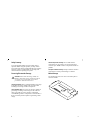
E stablished 1981
Advanced Test Equipment Rentals
www.atecorp.com 800-404-ATEC (2832)
User Manual
TDS3FFT
FFT Application Module
071-0349-01
*P071034901*
071034901
Copyright © Tektronix, Inc. All rights reserved.
Tektronix products are covered by U.S. and foreign patents,
issued and pending. Information in this publication supercedes
that in all previously published material. Specifications and
price change privileges reserved.
Tektronix, Inc., P.O. Box 500, Beaverton, OR 97077
TEKTRONIX, TEK, TEKPROBE, and Tek Secure are
registered trademarks of Tektronix, Inc.
DPX, WaveAlert, and e*Scope are trademarks of
Tektronix, Inc.
WARRANTY SUMMARY
Tektronix warrants that the products that it manufactures and
sells will be free from defects in materials and workmanship
for a period of one (1) year from the date of shipment from an
authorized Tektronix distributor. If a product proves defective
within the respective period, Tektronix will provide repair or
replacement as described in the complete warranty statement.
To arrange for service or obtain a copy of the complete
warranty statement, please contact your nearest Tektronix sales
and service office.
EXCEPT AS PROVIDED IN THIS SUMMARY OR THE
APPLICABLE WARRANTY STATEMENT, TEKTRONIX
MAKES NO WARRANTY OF ANY KIND, EXPRESS OR
IMPLIED, INCLUDING WITHOUT LIMITATION THE
IMPLIED WARRANTIES OF MERCHANTABILITY AND
FITNESS FOR A PARTICULAR PURPOSE. IN NO EVENT
SHALL TEKTRONIX BE LIABLE FOR INDIRECT,
SPECIAL OR CONSEQUENTIAL DAMAGES.
Contacting Tektronix
Product
Support
For questions about using Tektronix measurement
products, call toll free in North America:
1-800-833-9200
6:00 a.m. – 5:00 p.m. Pacific time
Or contact us by e-mail:
[email protected]
For product support outside of North America,
contact your local Tektronix distributor or sales
office.
Service
Support
Tektronix offers a range of services, including
Extended Warranty Repair and Calibration
services. Contact your local Tektronix distributor or
sales office for details.
Contents
Safety Summary . . . . . . . . . . . . . . . . . . . . . . . . . . . . 2
Installing the TDS3FFT Application Module . . . . . . . . 5
Introduction . . . . . . . . . . . . . . . . . . . . . . . . . . . . . . . 5
FFT Features . . . . . . . . . . . . . . . . . . . . . . . . . . . . . . . 6
Displaying an FFT Waveform . . . . . . . . . . . . . . . . . . . 7
FFT Math Menu . . . . . . . . . . . . . . . . . . . . . . . . . . . . . 8
FFT Windows . . . . . . . . . . . . . . . . . . . . . . . . . . . . . . 12
Aliasing . . . . . . . . . . . . . . . . . . . . . . . . . . . . . . . . . . . 14
FFT Examples . . . . . . . . . . . . . . . . . . . . . . . . . . . . . . 16
For a listing of worldwide service centers, visit our
web site.
Toll-free
Number
In North America:
1-800-833-9200
An operator can direct your call.
Postal
Address
Tektronix, Inc.
Department or name (if known)
P.O. Box 500
Beaverton, OR 97077
USA
Web Site
www.tektronix.com
1
Safety Summary
To avoid potential hazards, use this product only as
specified. While using this product, you may need to
access other parts of the system. Read the General Safety
Summary in other system manuals for warnings and
cautions related to operating the system.
Preventing Electrostatic Damage
CAUTION. Electrostatic discharge (ESD) can
damage components in the oscilloscope and its
accessories. To prevent ESD, observe these
precautions when directed to do so.
Handle Components Carefully. Do not slide sensitive
components over any surface. Do not touch exposed
connector pins. Handle sensitive components as little as
possible.
Transport and Store Carefully. Transport and store sensitive
components in a static-protected bag or container.
Manual Storage
The oscilloscope front cover has a convenient place to
store this manual.
Use a Ground Strap. Wear a grounded antistatic wrist strap
to discharge the static voltage from your body while
installing or removing sensitive components.
Use a Safe Work Area. Do not use any devices capable of
generating or holding a static charge in the work area
where you install or remove sensitive components.
Avoid handling sensitive components in areas that have a
floor or benchtop surface capable of generating a static
charge.
2
3
Installing the TDS3FFT Application Module
Refer to the TDS3000 & TDS3000B Series Application
Module Installation Instructions for instructions on
installing and testing the application module.
Introduction
The FFT application module adds FFT (Fast Fourier
Transform) measurement capabilities to your oscilloscope. The FFT process mathematically converts the
standard time-domain signal (repetitive or single-shot
acquisition) into its frequency components, providing
spectrum analysis capabilities.
Being able to quickly look at a signal’s frequency
components and spectrum shape is a powerful research
and analysis tool. FFT is an excellent troubleshooting aid
for:
H Testing impulse response of filters and systems
H Measuring harmonic content and distortion in
systems
H Identifying and locating noise and interference
sources
H Analyzing vibration
H Analyzing harmonics in 50 and 60 Hz power lines
4
5
FFT Features
Time Signals and FFT Waveforms Displayed Together
The FFT application module provides the following
features:
The time signals and FFT waveforms can be shown
together on the display. The time signal highlights the
problem; the FFT waveform helps you determine the
cause of the problem.
FFT Windows
Four FFT windows (Rectangular, Hamming, Hanning,
and Blackman-Harris) let you match the optimum
window to the signal you are analyzing. The Rectangular
window is best for nonperiodic events such as transients,
pulses, and one-shot acquisitions. The Hamming,
Hanning, and Blackman-Harris windows are better for
periodic signals.
Analyze Repetitive, Single-Shot, and Stored Waveforms
You can display an FFT waveform on any actively-acquired signal (periodic or one-shot), the last acquired
signal, or any signal stored in reference memory.
dB or Linear RMS Scales
The FFT vertical graticule can be set to either dB or
Linear RMS. A dB scale is useful when the frequency
component magnitudes cover a wide dynamic range,
letting you show both lesser and greater- magnitude
frequency components on the same display. A Linear
scale is useful when the frequency component magnitudes are all close in value, allowing direct comparison
of their magnitudes.
6
Displaying an FFT Waveform
1. Set the source signal Vertical SCALE so that the
signal peaks do not go off screen. Off-screen signal
peaks can result in FFT waveform errors.
2. Set the Horizontal SCALE control to show five or
more cycles of the source signal. Showing more
cycles means the FFT waveform shows more
frequency components, provides better frequency
resolution, and reduces aliasing.
If the signal is a single-shot (transient) signal, make
sure that the entire signal (transient event and ringing
or noise) is displayed and centered on the screen.
3. Push the Vertical MATH button to show the math
menu.
4. Push the FFT screen button to show the FFT side
menu.
5. Select a signal source. You can do an FFT on any
channel or any stored reference waveform.
6. Select the appropriate vertical scale and FFT window.
7. Use zoom controls and the cursors to magnify and
measure the FFT waveform.
7
FFT Math Menu
H Signals that have a DC component or offset can cause
incorrect FFT waveform component magnitude
values. To minimize the DC component, choose AC
Coupling on the source signal.
Bottom
Side
Description
FFT
Set FFT
Source to
Sets the FFT signal source.
Valid input sources are Ch 1
and Ch 2 (2-channel instruments), Ch 1 through Ch 4
(4-channel instruments), and
Ref 1 through Ref 4 (all instruments).
H To reduce random noise and aliased components in
repetitive or single-shot events, set the oscilloscope
acquisition mode to average over 16 or more samples.
Average mode attenuates signals not synchronized
with the trigger.
Set FFT Vert
Scale to
Sets the display vertical scale
units. Available scales are
dBV RMS and Linear RMS.
Sets which window function
(Hanning, Hamming, BlackmanHarris, or Rectangular) to apply
to the source signal. Refer to
page 12 for more FFT window
information.
H Do not use Peak Detect and Envelope modes with
FFT. Peak Detect and Envelope modes can add
significant distortion to the FFT results.
Set FFT
Window to
FFT Source Key Points
H Do not use the Average acquisition mode if the
source signal contains frequencies of interest that are
not synchronized with the trigger rate.
H For transient (impulse, one-shot) signals, set the
oscilloscope to trigger on the transient pulse in order
to center the pulse information in the waveform
record.
H Push the side menu button to select the source.
H Using FFT slows down the oscilloscope’s response
time in Normal acquisition mode (10k record length).
H A waveform acquired in Normal acquisition mode
has a lower noise floor and better frequency
resolution than a waveform acquired in Fast Trigger
mode.
8
9
FFT Vertical Scale Key Points
H Push the side menu button to select a scale. Available
scales are dBV RMS and Linear RMS.
H Use the Vertical POSITION and SCALE knobs to
vertically move and rescale the FFT waveform.
H To display FFT waveforms with a large dynamic
range, use the dBV RMS scale. The dBV scale
displays component magnitudes using a log scale,
expressed in dB relative to 1 VRMS, where 0 dB =1
VRMS, or in source waveform units (such as amps for
current measurements).
H To display FFT waveforms with a small dynamic
range, use the Linear RMS scale. The Linear RMS
scale lets you display and directly compare
components with similar magnitude values.
Nyquist Frequency Key Point
H To determine the Nyquist frequency, push the
ACQUIRE menu button. This displays the current
sample rate on the bottom right area of the screen.
The Nyquist frequency is one-half of the sample rate.
For example, if the sample rate is 25.0 MS/s, then the
Nyquist frequency is 12.5 MHz.
Zooming an FFT Display. Use the Zoom button
,
along with horizontal POSITION and SCALE controls,
to magnify FFT waveforms. When you change the zoom
factor, the FFT waveform is horizontally magnified
about the center vertical graticule, and vertically magnified about the math waveform marker. Zooming does not
affect the actual time base or trigger position settings.
NOTE. FFT waveforms are calculated using the
entire source waveform record. Zooming in on a
region of either the source or FFT waveform
will not recalculate the FFT waveform for that
region.
Measuring FFT Waveforms Using Cursors. You can use
cursors to take two measurements on FFT waveforms:
magnitude (in dB or signal source units) and frequency
(in Hz). dB magnitude is referenced to 0 dB, where 0 dB
equals 1 VRMS. Use horizontal cursors (H Bars) to
measure magnitude and vertical cursors (V Bars) to
measure frequency.
Magnitude cursors
10
Frequency cursors
11
FFT Windows
Applying a window function to the source waveform
record changes the waveform so that the start and stop
values are close to each other, reducing FFT waveform
discontinuities. This results in an FFT waveform that
more accurately represents the source signal frequency
components. The ’shape’ of the window determines how
well it resolves frequency or magnitude information.
FFT Window
Characteristics
Best for measuring
BlackmanHarris
Best magnitude,
worst at resolving
frequencies.
Predominantly single frequency waveforms to look
for higher order harmonics.
Hamming,
Hanning
Better frequency,
poorer magnitude
accuracy than
Rectangular.
Hamming has
slightly better frequency resolution
than Hanning.
Sine, periodic, and narrowband random noise.
Best frequency,
worst magnitude
resolution. This is
essentially the
same as no window.
Transients or bursts where
the signal levels before and
after the event are nearly
equal.
Source
waveform
Waveform
data points
×
=
Rectangular
Point-by-point
multiply
Window
function
(Hanning)
Source waveform
after windowing
Transients or bursts where
the signal levels before and
after the event are significantly different.
Equal-amplitude sine waves
with frequencies that are
very close.
Broad-band random noise
with a relatively slow varying
spectrum.
FFT
With windowing
12
13
Aliasing
Problems occur when the oscilloscope acquires a signal
containing frequency components that are greater than
the Nyquist frequency (1/2 the sample rate). The frequency components that are above the Nyquist frequency are undersampled and appear to “fold back” around
the right edge of the graticule, showing as lower frequency components in the FFT waveform. These incorrect
components are called aliases.
Nyquist frequency
(½ sample rate)
0 Hz
H Use a filter on the source signal to bandwidth limit
the signal to frequencies below that of the Nyquist
frequency. If the components you are interested in are
below the built-in bandwidth settings (20 MHz
bandwidth for all oscilloscopes, 150 MHz bandwidth
for 300 MHz and 500 MHz oscilloscopes), set the
source signal bandwidth to the appropriate value.
Push the Vertical MENU button to access the source
channel bandwidth menu.
Amplitude
Frequency
If the increased number of frequency components
shown on the screen makes it difficult to measure
individual components, use the Zoom button to
magnify the FFT waveform.
Aliased frequencies
Actual frequencies
Use the following methods to eliminate aliases:
H Increase the sample rate by adjusting the Horizontal
SCALE to a faster frequency setting. Since you
increase the Nyquist frequency as you increase the
horizontal frequency, the aliased frequency
components should appear at their proper frequency.
14
15
FFT Examples
T
FFT Example 1
A pure sine wave can be input into an amplifier to
measure distortion; any amplifier distortion will
introduce harmonics in the amplifier output. Viewing the
FFT of the output can determine if low-level distortion is
present.
You are using a 20 MHz signal as the amplifier test
signal. You would set the oscilloscope and FFT parameters as listed in the table:
1
1
2
3
FFT Example 1 Settings
Control
Setting
CH 1 Coupling
AC
Acquisition Mode
Average 16
Horizontal Resolution
Normal (10k points)
Horizontal SCALE
100 ns
FFT Source
Ch 1
FFT Vert Scale
dBV
FFT Window
Blackman-Harris
16
M
The first component at 20 MHz (figure label 1) is the
source signal fundamental frequency. The FFT waveform also shows a second-order harmonic at 40 MHz (2)
and a fourth-order harmonic at 80 MHz (3). The presence of components 2 and 3 indicate that the system is
distorting the signal. The even harmonics suggest a
possible difference in signal gain on half of the signal
cycle.
17
FFT Example 2
T
Noise in mixed digital/analog circuits can be easily
observed with an oscilloscope. However, identifying the
sources of the observed noise can be difficult.
The FFT waveform displays the frequency content of the
noise; you may then be able to associate those frequencies with known system frequencies, such as system
clocks, oscillators, read/write strobes, display signals, or
switching power supplies.
The highest frequency on the example system is
40 MHz. To analyze the example signal you would set
the oscilloscope and FFT parameters as listed in the
following table:
1
2
M
FFT Example 2 Settings
Control
Setting
CH 1 Coupling
AC
Acquisition Mode
Sample
Horizontal Resolution
Normal (10k points)
Horizontal SCALE
4.00 ms
Bandwidth
150 MHz
FFT Source
Ch 1
FFT Vert Scale
dBV
FFT Window
Hanning
18
1
Note the component at 31 MHz (figure label 1); this
coincides with a 31 MHz memory strobe signal in the
example system. There is also a frequency component at
62 MHz (figure label 2), which is the second harmonic
of the strobe signal.
19
20