1
Waveform analysis tools in seismology
SeismoGRAPHer
FOR WINDOWS
(V.3.7.4)
User Manual
Sgraph© 2008-2010
Programmed by
Dr. Mohamed Farouk Abdelwahed
National Research Institute of Astronomy and Geophysics
(NRIAG)-Egypt
2008-2010
Waveform Analysis Tools in Seismology
2
_________________________________________________________________________________
____________________________________________________________________________________
Sgraph V3.7 – User Manual
3
Waveform Analysis Tools in Seismology
_________________________________________________________________________________
About Sgraph
____________________________________________________________________________________
Sgraph V3.7 – User Manual
Waveform Analysis Tools in Seismology
4
_________________________________________________________________________________
Table of content
Preface ........................................................................................................ 10
Sgraph descriptions ............................................................................... 10
How to install: ........................................................................................ 12
Program arguments:.............................................................................. 12
File opening and filters .......................................................................... 13
File acceptance ....................................................................................... 13
Data insertion ......................................................................................... 15
Typing rules: ......................................................................................................... 15
Trace Selection ....................................................................................... 15
Single trace selection: ........................................................................................... 16
Multiple trace selection: ....................................................................................... 16
Menu ........................................................................................................... 17
1 File ........................................................................................................ 17
1.1 Load: ................................................................................................................ 17
1.2 New: ................................................................................................................. 18
1.2.1 Data format .............................................................................................. 18
1.2.2 Multi-column Data dialog box: .............................................................. 21
1.2.3 Data information: .................................................................................... 22
1.2.4 Green’s Function dialog box................................................................... 26
1.3 Open station .................................................................................................... 28
1.4 Delete ............................................................................................................... 29
1.5 Info ................................................................................................................... 29
1.6 Edit Data.......................................................................................................... 29
1.7 Setup ................................................................................................................ 30
1.8 PS preferences. ................................................................................................ 32
1.9 Save data: ........................................................................................................ 33
1.9.1
Save One-Column ASCII data (Sgraph 3.0 Y-format) .............. 33
1.9.2
Save Two-Column ASCII data (Sgraph 3.0 XY-format) .............. 33
1.9.3
Save Binary SAC format.................................................................. 34
1.9.4
Save SAN Format (Seismic ANalysis format) ................................ 34
1.9.5
Save GSE (INT) and (CM6) format ................................................ 34
1.9.6
Save WAV format............................................................................. 35
1.10 Save as BMP .................................................................................................. 35
____________________________________________________________________________________
Sgraph V3.7 – User Manual
5
Waveform Analysis Tools in Seismology
_________________________________________________________________________________
1.11 Save as PS ...................................................................................................... 35
1.12 Print ............................................................................................................... 36
1.13 Quit ................................................................................................................ 36
2. Routine tools ....................................................................................... 37
2.1 Zoom ................................................................................................................ 37
2.2 Tapering .......................................................................................................... 37
2.3 Fast Fourier ..................................................................................................... 37
2.4 Inv. Fourier ..................................................................................................... 38
2.5 Phase Trans. .................................................................................................... 38
2.6 Envelop Trans ................................................................................................. 39
2.7 Hilbert transform ........................................................................................... 39
2.8 Integration ....................................................................................................... 39
2.9 Differentiation ................................................................................................. 39
2.10 Rotation ......................................................................................................... 39
2.11 Add noise ....................................................................................................... 40
2.12 Plot Mecha ..................................................................................................... 41
2.13 Wadati diagram ............................................................................................ 42
2.14 Magnitude ..................................................................................................... 43
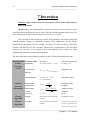
3 Filter ..................................................................................................... 46
3.1 Hipass............................................................................................................... 47
3.2 Lowpass ........................................................................................................... 47
3.3 Bandpass .......................................................................................................... 47
3.4 PoleZero........................................................................................................... 47
4 Math ..................................................................................................... 49
4.1 Power order ..................................................................................................... 49
4.2 Multiplication .................................................................................................. 49
4.3 Area under curve ............................................................................................ 49
4.4 Normalization ................................................................................................. 50
4.5 Absolute ........................................................................................................... 50
4.6 Cumulative Sum ............................................................................................. 50
4.7 CrossCalc......................................................................................................... 50
4.8 Spectral Ratio.................................................................................................. 51
4.9 Power Spectrum.............................................................................................. 51
4.10 Cross Spectrum ............................................................................................. 51
4.11 Cross correlation .......................................................................................... 52
4.12 Multi Cross correlation ................................................................................ 52
4.13 Auto correlation ............................................................................................ 53
4.14 Convolution ................................................................................................... 53
4.15 Deconvolution ............................................................................................... 53
____________________________________________________________________________________
Sgraph V3.7 – User Manual
Waveform Analysis Tools in Seismology
6
_________________________________________________________________________________
4.16 Distribution ................................................................................................... 53
4.17 Statistics ......................................................................................................... 54
4.18. Resampling ................................................................................................... 54
4.19. Calculator ..................................................................................................... 54
5 Correction ............................................................................................ 55
5.1 Instrumental .................................................................................................... 55
5.2 Site correction ................................................................................................. 55
5.3 Remove DC...................................................................................................... 55
5.4 Remove O.T..................................................................................................... 56
5.5 Reduce T.T ...................................................................................................... 56
6 Test Signal ........................................................................................... 57
6.1 Line .................................................................................................................. 57
6.2 Spike................................................................................................................. 57
6.3 Step Function .................................................................................................. 58
6.4 Sine/Cosine wave ............................................................................................ 58
6.5 Brune disp/vel ................................................................................................. 58
6.6 Sweep ............................................................................................................... 59
6.7 Mixed ............................................................................................................... 59
6.8 Polynomial ....................................................................................................... 59
6.9 Trapezoid......................................................................................................... 60
6.10 Noise Signal ................................................................................................... 60
7 Inversion .............................................................................................. 61
7.1 Linear fit (SVD) .............................................................................................. 62
Polynomial function: ................................................................................ 62
Arrival time vs distance relation: ............................................................ 62
Wadati diagram: S-P time = a0 + a1*T ................................................ 63
7.2 Nonlinear fit (Marquard)............................................................................... 64
How to fit a spectral trace with Brune model ................................................ 64
Source Parameters estimation: ....................................................................... 65
7.3 PGV-Dist relation : (Peak ground velocity- distance relation) ...................... 67
8 PhaseID ................................................................................................ 68
Phase data sources:............................................................................................... 68
1-Green function file: ..................................................................................... 68
2-Travel time table: .......................................................................................... 68
8.1 Search Phase ................................................................................................... 68
8.2 Insert Phase ..................................................................................................... 69
8.3 Compare Phase ............................................................................................... 71
8.4 Save Phases...................................................................................................... 72
____________________________________________________________________________________
Sgraph V3.7 – User Manual
7
Waveform Analysis Tools in Seismology
_________________________________________________________________________________
8.5 Load Table ...................................................................................................... 73
9 Picking .................................................................................................. 74
9.1 Pick/Del Phases ............................................................................................... 75
Change trace: .................................................................................................... 75
Pick phase automatically: ................................................................................ 75
Pick phase manually: ....................................................................................... 75
Modify Phase: ................................................................................................... 76
Delete Phase(s): ................................................................................................. 76
Assign Phases: ................................................................................................... 77
Amplitude picking: ........................................................................................... 77
9.2 Auto Picking .................................................................................................... 78
9.3 S-Pick Calc. ..................................................................................................... 78
9.4 Assigning Phases ............................................................................................. 78
9.5 MCCC .............................................................................................................. 79
How to see results: ............................................................................................ 81
How to confirm picking: .................................................................................. 82
9.6 Delete Picking.................................................................................................. 83
9.7 Load Picking ................................................................................................... 83
9.8 Load SAC Picking .......................................................................................... 83
9.9 Save Picking .................................................................................................... 83
10 Synthetic ............................................................................................ 85
10.1 GRT (Generalized Ray Theory) .................................................................. 85
Model file:.................................................................................................. 85
Ray file:...................................................................................................... 85
10.2 Wave Number (Discrete Wave Number method): .................................... 87
10.3 Modeling: ....................................................................................................... 89
General strategy: .............................................................................................. 90
Model parameters: ........................................................................................... 93
Model parameter space .................................................................................... 94
Fitness function:................................................................................................ 95
Dialog buttons description: .............................................................................. 95
How to perform waveform modelling: ........................................................... 97
Additional option. ............................................................................................. 98
Travel time joint modelling: ............................................................................ 98
Important notes for waveform modelling: ..................................................... 99
10.4 EMPIRE (for restricted versions only): ................................................... 100
How to do EMPIRE........................................................................................ 100
10.5 ASPO (for restricted versions only) .......................................................... 100
What is ASPO ? .............................................................................................. 100
____________________________________________________________________________________
Sgraph V3.7 – User Manual
Waveform Analysis Tools in Seismology
8
_________________________________________________________________________________
How to do ASPO ............................................................................................. 101
10.6 Model to GRF: ............................................................................................ 103
10.7 Path to BLN: ............................................................................................... 103
11 Attenuation ...................................................................................... 105
11-1 Qs Spectral ratio: Single station method, Giampiccolo et al., 2007) ..... 105
11-2 MLTW (Multiple Lag Time Window technique, Hoshiba (1993) ......... 106
MLTW overview ............................................................................................. 106
11-3 MLTW_INV ............................................................................................... 112
12 Site effect .......................................................................................... 113
12.1 Inversion method ........................................................................................ 113
13 Graph ............................................................................................... 116
13.1 Draw All ...................................................................................................... 116
13.2 Draw Spec.................................................................................................... 116
13.3 Multitrace .................................................................................................... 117
13.4 Overlay ........................................................................................................ 117
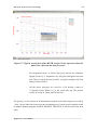
13.5 Record section ............................................................................................. 118
13.6 Rearrange .................................................................................................... 121
13.7 Sort ............................................................................................................... 122
13.8 Merge ........................................................................................................... 122
13.9 Align ............................................................................................................. 122
13.10 Navigate ..................................................................................................... 123
13.11 Compare .................................................................................................... 123
14 Location ........................................................................................... 126
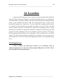
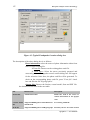
14.1 Hypoinverse................................................................................................. 126
How to locate an earthquake ......................................................................... 128
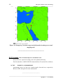
14.2 Genmap: Plot a location map of a customized event............................... 129
14.3 Plot map: Execute the Postscript viewer to show a map......................... 130
References ................................................................................................ 131
List of Figures .......................................................................................... 133
Appendix 1 ............................................................................................... 136
Appendix 2 ............................................................................................... 137
Appendix 3 ............................................................................................... 138
Appendix 4 ............................................................................................... 143
Appendix 5 ............................................................................................... 145
Appendix 6 ............................................................................................... 146
Appendix 7 ............................................................................................... 147
Appendix 8 ............................................................................................... 149
Appendix 9 ............................................................................................... 150
____________________________________________________________________________________
Sgraph V3.7 – User Manual
9
Waveform Analysis Tools in Seismology
_________________________________________________________________________________
Sgraph Limitations: ........................................................................ 151
____________________________________________________________________________________
Sgraph V3.7 – User Manual
Waveform Analysis Tools in Seismology
10
_________________________________________________________________________________
Preface
Sgraph descriptions
Sgraph is a program for Seismological data analysis. It provides facilities to plot
and analyse different types of data format. It is a FORTRAN Quick-Win application in
which dialogs are used to easily read and write information. The FORTRAN graphic
libraries are used for the plotting routine. In addition, Post Script facilities are inserted
to obtain a PS version of the Sgraph plotting.
The idea of writing this program comes during my master study. I faced a lot of
problems to analyse the data of the only digital seismographic station (KEG) in Egypt at
that time. The data of this station has a special format that needs to be reformatted to fit
in the available software at that time (PITSA). Pitsa helps a lot. But every time I use it I
need to reformat my data. The idea of Pitsa attracts me so much in a way I decided to
make a similar plotting program just for reading my own unique format. The idea grows
up until the Quick-Win FORTRAN comes to my hand. Sgraph starts and step by step I
insert all subroutines I need to establish my PhD study. I decided to insert all the
required data formats that I met to make it easier for the researchers to read and analyse
data. Finally, I found Sgraph a special program in seismology and I realize that it is
important to be released for researchers, and here it is.
In this version, the program read the data format of the types ASCII SAC,
Binary SAC, Multicolumn ASCII data, GSE formats, Y-format (Nanometrics), and
Focal mechanism files..
The program provides the principle waveform analysis tools such as, Zooming,
Integration, Differentiation, Filtering, FFT, Convolution, Correlation, ..etc.
Inversion processes are utilized in Sgraph to solve either linear or nonlinear
seismological problems. SVD (Singular Value Decomposition) tools are used for the
linear problems (e.g. travel time/slowness, Wadati Diagram, and others). Marquard
inversion tools are used to solve the nonlinear problems (i.e., Brune models, Q vs Freq,
MLTW, and others (see text below for detail). Global optimization method represented
____________________________________________________________________________________
Sgraph V3.7 – User Manual
11
Waveform Analysis Tools in Seismology
_________________________________________________________________________________
by Genetic Algorithm is implemented for waveform modelling, MLTW inversion, and
PGV-distance relation.
Intensive tools for constructing synthetic seismograms and waveform
modelling are provided. The Generalized Ray Theory (GRT) and Discrete Wave
Number (DWN) methods are available in Sgraph in a simple way. The waveform
modeling process is performed in Sgraph through many advanced tools such as,
Genetic Algorithm (GA), GRT, Navigation, Comparison, and others.
Phase identification tools are also included in special routines like Insert phase,
Search phase, Compare phases and others. Comprehensive tools for manual and Auto
phase picking are provided.
The earthquake hypocentral location tool is newly inserted in this version. The
picking tool and the station info provide the required information to accomplish a
complete hypocentral location procedure by using the hypoinv2000 code that is directly
linked with Sgraph. A GMT (Generic Map Tools) script available and automatically
executed to generate a PS plot of the hypocentral map with the event location and its
information (The GMT package should be installed for the mapping tools).
Restricted versions of Sgraph provides some advanced techniques not available
in the free versions, those techniques are, the ASPO technique for focal mechanism
estimation; spectral and inversion method for Site effect estimation; The Multiple Lag
Time Window (MLTW) technique and Q-coda method for attenuation study. All those
techniques are discussed in detail in this manual.
One important feature of Sgraph is the variety of the output data type. Sgraph
maintains the ‘Saving’ of the analysed waveforms in many ways. The whole analysed
traces can be either saved in one compressed binary file “SAN” (Seismic ANalysis file)
to be used later; or saved individually in one- or two-column ASCII data files to be
plotted in other plotting programs; or it can be saved in SAC format to be read by
“SAC” program (Seismic Analysis Code) for further analysis. Saving data as GSE (INT
and CM6) and WAV formats are also included. An audio (WAV) copy of the recorded
traces can also be obtained.
In general, Sgraph consists of useful tools to perform successful researches in
waveform analysis. Some parts look like the “SAC” program (William, et al. 1990),
other parts like “Pitsa” (Franck and James, 1992). However, the integration of all the
principle tools with the Sgraph tools makes Sgraph special. Many parts of this code are
____________________________________________________________________________________
Sgraph V3.7 – User Manual
Waveform Analysis Tools in Seismology
12
_________________________________________________________________________________
taken from different sources like Numerical recipes, Seismic Analysis Code (SAC),
Seisan code, and some others.
Zooming, Navigation and Picking tools are modified in this version for a better
usage of mouse and keyboard control.
How to install:
The installation disk consists of the Sgraph setup file necessary to
install the Sgraph package in your system. For the location purpose, the GMT
package and PostScript viewer are included as well. The user has to install
them individually if it doesn’t installed in the System.
To install Sgraph package, do the following:
- Launch the installation file: Sgraph_setup.exe
- Follow the setup procedures to save the application in the desired location.
N.B. This version is only valid for the win32 windows systems platform. (Win95, Win98,
Win98SE, Win2000, WinXp, Vista).
Program arguments:
Sgraph can read file names of different formats by passing through arguments.
Using the console window, or Windows Commander, a file can be opened by
Sgraph directly by typing its name after the Sgraph launching command.
-
From the Sgraph working folder, type “Sgraph” following by space following by
the filename(s) to open.
The file could be of any type. Sgraph, in this version, automatically detects the type
of file and open it by the appropriate way.
EX: To open the file “green.sac” by Sgraph.
Simply type:
” Sgraph green.sac “
____________________________________________________________________________________
Sgraph V3.7 – User Manual
13
Waveform Analysis Tools in Seismology
_________________________________________________________________________________
The description of the different file formats supported by Sgraph will be discussed in
the next sections.
Because the Sgraph supports a wide range of file types, it is convenient to
associate the different file extensions to Sgraph. This can be done using the windows
explorer folder option or the windows commander (see the OS helping manual for how
to do). Use icons provided by Sgraph for the corresponding data formats, this makes it
easier to distinguish the different data formats from among the variety of files in the
working folder. Once this is done, the specified files can be opened directly by Sgraph
by double click on it.
N.B. Every time a file is opened this way, a new Sgraph program will be launched. This
will exhaust the computer memory. It is recommended to close the old Sgraph before
open another file.
File opening and filters
Multifile opening: Sgraph gives the ability to open multiple files simultaneously.
Selection is done following windows way. Up to 200 files can be selected at once.
Sgraph will ask for the required parameters file by file.
Filter specification: From the filter box, a specific file terminals (wildcard) can be
requested (e.g. *.uer,*.001, etc...). This is useful for reading a specific file types among
a big number of files.
File acceptance
For managing the Computer memory, Sgraph has two types of memory
storage; a temporary storage for the files just being read and locatable storage for
the accepted files.
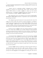
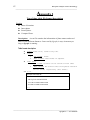
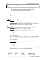
For files just being read or being processed a dialog asking for (Add, Replace,
Repeat, Ignore) is appeared for managing traces (See the next figure).
____________________________________________________________________________________
Sgraph V3.7 – User Manual
Waveform Analysis Tools in Seismology
14
_________________________________________________________________________________
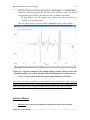
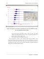
Figure 1: Process/trace Accept dialog box
The “All” check box controls the multitrace entry. If checked, the selected value
(or process) will be applied to all coming traces (e.g. Add all, Replace all, Ignore all).
To add a specific window only use zoom button. See the next table.
The button 'Put in Memory' serves to add the current trace in a temporary
memory (Buffer) to be used for further analysis. The idea of this buffer is to use the
current trace in another tools on air, or without put it in the main memory. It is
important to say that this buffer stores only one trace. The user has not to use it for
routine that requires multiple traces. Moreover, the user have to finish work with the
trace in memory before opening a trace from disk or do a single trace selection (Sgraph
buffer is used internally for memory management). To continue work with the trace in
memory, select Memory button from the select trace dialog (see the section of single
trace selection below).
All (Checked)
Add
Replace
Ignore
Repeat
Put in
memory
Add all traces
Replace all traces (this will delete all the old
traces)
Ignore all traces (this will ignore all the
coming traces in operation)
………………………………………..
All (not Checked)
Ask again for the coming traces
Ask again for the coming traces
Ask again for the coming traces
If during reading file: Open a new file.
If during a procedure: Repeat the procedure.
Put the current trace in temporary memory (not added to work screen). The user can apply
any of the Sgraph tools on it before add it to the permanent memory.
In case the Replace button in clicked the following check boxes are taken into consideration :
Replace plot : Force the replacement of all the current traces = delete all
before open
Replace trace: Normal case, replace the current trace.
____________________________________________________________________________________
Sgraph V3.7 – User Manual
15
Waveform Analysis Tools in Seismology
_________________________________________________________________________________
Custom replace: Force to replace a customized trace.
Data insertion
For the interaction between “user” and Sgraph, a dialog box is used. This
dialog is the main way to insert the required parameters needing for the requesting
process.
The insertion of data has different types; single value entry, and multiple values
entry. For that, specific typing rules are used.
Typing rules:
1- For one value data: Value should be a number (real or integer). Any
character is not permitted.
2- For multiple value data: Values should be numbers separated by spaces or
comas.
3- Some tools require mathematical operators; only (+,-,*,/,^) are permitted
(Spaces are not permitted with this).
4- If asking for trace indices, values should be within the plotted trace range.
5- For range of data: Type the two data limits separated by ’:’.
EX: [1:10] = from 1 to 10.
6- For selecting all traces: Type '0'. This is a special request when asking for
applying the process on all traces. For example when delete, [0] means,
delete all. (Notice, this is applied only when asked about trace indices).
7- No parentheses or spaces with separators are permitted.
N.B. The permitted separator characters are [+-*/^ :,].
For bad typing, an error message will appear.
Trace Selection
Because of the different tools included in Sgraph, some of these tools are
applied to a single trace, other tools are applied to multitraces and others can be
applied to both cases. For that, the trace selection will differs from a tool to
another. Sgraph uses two dialogs to receive trace selection.
____________________________________________________________________________________
Sgraph V3.7 – User Manual
Waveform Analysis Tools in Seismology
16
_________________________________________________________________________________
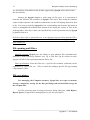
Single trace selection:
Select a single trace from the box given in the following dialog box.
Figure 2: Single trace selection dialog box
the Memory button serves to select the trace that was stored in temporary memory
instead of the conventional traces in the working memory. To store trace in memory, see
the above 'Add trace' section.
Multiple trace selection:
This is similar to the data insertion dialog but instead it deals with trace indices.
This also accepts (0) as select all traces.
_________________________
____________________________________________________________________________________
Sgraph V3.7 – User Manual
17
Waveform Analysis Tools in Seismology
_________________________________________________________________________________
Menu
These are the complete functions and tools included in Sgraph. These tools can not
be accessed from other place instead of the main menu (In this version). Here we
will describe the different tools and techniques provided in the form of 'Menu' and
'How to do'.
1 File
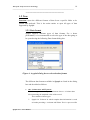
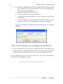
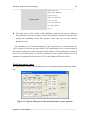
1.1 Load:
Function: Load the previously saved SAN file (Seismic ANalysis file).
It is a specific binary file written by Sgraph. It consists of the complete
information of the traces previously saved. (i.e., number of points, sampling rate, scales,
trace names, data limits, azimuth, distance, etc.). Single event or multiples of events
might be saved as SAN file. This is useful for saving the processed data for further
analysis. See the Save menu for how to save a SAN file.
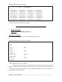
Select as much SAN files as required, then the following dialog box will appear
listing event names and the corresponding stations existing in the selected files. Use the
station name wildcard and component check boxes to retrieve specific station names
and components.
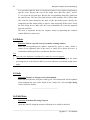
Figure 3: A typical dialog box to retrieve the data from SAN file(s).
____________________________________________________________________________________
Sgraph V3.7 – User Manual
Waveform Analysis Tools in Seismology
18
_________________________________________________________________________________
____________________________
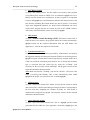
1.2 New:
Function: Open the different formats of data from a specific folder to be
plotted and analyzed. This is the main routine to open all types of data
supported by Sgraph.
1.2.1 Data format
Sgraph supports different types of data formats. For a better
performance, it is recommended to select the type of the data going to
be opened using the following Data format dialog box.
Figure 4: A typical dialog box to select the data format.
The different data formats available in Sgraph are listed in the dialog
box and described as follows:
One- Column/auto ASCII format:
This format type is used to open an unknown data or a 1-Column data
file representing the amplitude value of the record.
This could be of three types:
1.
Sgraph 3.0 Y-format. In which complete data information is saved
as header preceding a 1-column ASCII data. This is a pre-saved file
____________________________________________________________________________________
Sgraph V3.7 – User Manual
19
Waveform Analysis Tools in Seismology
_________________________________________________________________________________
by Sgraph. It is automatically identified once open the file by any
ASCII type.
2.
Any 1-Column data file with or without header. The header will be
automatically skipped by Sgraph. The value read represents the
Y-Axis or amplitude value of the trace. Time axis is calculated
according to the sampling rate inserted by the user in the info
dialog box during the file opening.
3. Unknown ASCII files of single or multi-columns. If multi-column
data, a special dialog box will appear to show a part of data and to
specify the columns corresponding to X and Y axis. The typical
multicolumn dialog box is shown below. (Notice, multicolumn
data should be only numbers).
Two-Column/auto ASCII format:
This format type used to open an unknown data or a 2-Column data file.
This could be of three types:
1.
Sgraph 3.0 XY-format. In which complete data information is
saved as header preceding a 2-column ASCII data. This is a
pre-saved file by Sgraph. It is automatically identified once
opened by any ASCII type format.
2.
Any 2-Column data file with or without header. The header
will be automatically skipped by Sgraph. The value read
represents the time and amplitude values of the trace. The
sampling rate is automatically calculated from the data and
assigned to the trace. No need for any additional information
corresponding to the trace of this type.
3.
Unknown ASCII files of single or multi-columns. Same as the
above one-column data format.
Mednet Format:
To force the program to read a MedNet Very Broadband seismic network
format. It is an ASCII file consisting of a header and 8 column data. The
program extracts all the required information from the header.
SAC ASCII format:
To open an SAC ASCII data format. The file could be pre-saved by SAC
program or any ASCII SAC format in UNIX or PC environment. The
program extracts all the required information from the SAC headers.
____________________________________________________________________________________
Sgraph V3.7 – User Manual
Waveform Analysis Tools in Seismology
20
_________________________________________________________________________________
SAC Binary format:
To open a SAC Binary format. The file could be pre-saved by SAC program
or any Binary SAC format in UNIX or PC environment. Sgraph can save a
Binary SAC file format to be read directly by SAC program. It is important
to notice that Sgraph saves all information related to the analysed trace in the
SAC headers including the Picked Phases (the first 9 phases), event name,
origin time, Magnitude, Moment, etc. Some of this information can not be
read by SAC program because it is stored in some of the “USER” headers.
This newly stored information can be read only by Sgraph.
GSE format:
To open a Global Seismic Exchange (GSE) file format in either INT or
CM6 formats. If not known, the program detects the format automatically.
Sgraph extracts all the required information from the GSE header. See
appendices 7, 8 for the description of GSE format.
Y-format (nanometrics):
To open Y-format data. This format provided by “Nanometrics” and used by
the Egyptian National Seismological Network (ENSN) as the storing format.
Sgraph can open Y-format data of ASCII type directly and plot all the file if
it did not exceed the maximum point allowed. The Y-format file of Binary
type is converted first into ASCII type by using the “Y5dump” code
necessary for this case (this is done internally). The program extracts all the
required information from the header.
Note: Make sure that the “Y5dump” code and its “lib,dll’s “ files exist is the
folder (“installing folder”¥bin¥). This is done automatically when install
Sgraph in the proper way (See above how to install Sgraph).
PITSA format:
To open a PITSA file format. This format is Pitsa specific format in which
data is stored in 1-column ASCII data preceding by headers corresponding to
the trace start date, Sampling rate, Number of points, etc. This format is
automatically recognized by Sgraph. The program extracts all the required
information from the header.
Green Function format:
To open a pre-saved Green function file. This is a Sgraph specific format
generated from the GRT tool. (See Appendix 4 for detail). Sgraph gives the
____________________________________________________________________________________
Sgraph V3.7 – User Manual
21
Waveform Analysis Tools in Seismology
_________________________________________________________________________________
green’s function dialog needed for the insertion of the synthetic seismogram
parameters.
Focal mechanism Plot:
To plot a pre-saved Focal mechanism file. This is a Sgraph specific
format generated from the Mecha tools..
Table summarizing the different data format supported by Sgraph:
#
Data Format
1
1- Column/auto ASCII
2
2- Column/auto ASCII
Description
Unknown or a 1-column data file represents the amplitude value of the
record.
Unknown or a 2-column data file. The first column is the time and the
second column is the amplitude. Sampling rate is automatically calculated.
The MedNet Very Broadband seismic network format. It is an ASCII file
3
MedNet
consists of a header and 8 column data. The program extracts all
information needing from the header.
4
SAC ASCII
The SAC ASCII format. No need to insert any information.
5
SAC BINARY
The SAC BINARY format, No need to insert any information.
6
GSE
7
Y-format (Nanometrics)
Y-format from Nanometrics either Binary or ASCII type.
8
PITSA
PITSA format. The program detects the format automatically.
9
Green Function
GSE format either INT or CM6. The program detects the format
automatically.
The generalized ray theory green’s function format. (See Appendix 3 for
detail).
A specific focal mechanism text format. This is Sgraph pre-saved file. It
represent the stereographic projection of a given strike, dip and slip of fault
10
Focal mechanism Plot
planes. Many planes can be presented simultaneously and can be plotted in
any plotting software as discontinuous X,Y data. See Focal mechanism
section for detail.
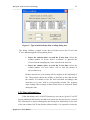
1.2.2 Multi-column Data dialog box:
The multi-column data requires a special way to manipulate the data
columns and to specify the columns to plot. This is done by using following
dialog box:
____________________________________________________________________________________
Sgraph V3.7 – User Manual
Waveform Analysis Tools in Seismology
22
_________________________________________________________________________________
Figure 5: Typical multicolumn data reading dialog box.
The dialog exhibits a sample of the data read and receives the X-Axis and
Y-Axis data through the corresponding boxes.
Insert the column where to read the X-axis data: Select the
column number of X-axis. Select “Construct” to generate the
X-axis from the sampling rate value entered in the info box.
Insert the column where to read the Y-axis data: Select the
column number of Y-axis. Select “All” to read all columns in
trace/column way.
Headers and uneven row formats will be skipped in the beginning of
file. The program checks the validity of data line by line and decides
the number of columns in the file and read them accordingly and
associates every trace with its corresponding column. The program
stops reading when a change in data format occurs or characters found
among the data.
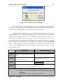
1.2.3 Data information:
If the data being read is of ASCII format type (except the Sgraph X and XY
format) additional information needed to be inserted to plot the trace(s) correctly.
This information is inserted through the Info dialog box. Particularly, in the case
of the one-column ASCII data format without header, it is required to insert the
____________________________________________________________________________________
Sgraph V3.7 – User Manual
23
Waveform Analysis Tools in Seismology
_________________________________________________________________________________
sampling rate of the trace being read (Default is 100 samples per sec).
Sometimes, it is necessary to skip some points (Nskip) from the beginning of file
or read a specific number of points (Nread). The Nskip and Nread and many
other information related to station or event can be inserted through the Info
dialog box.
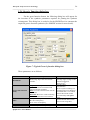
Info dialog box:
This dialog is the main dialog box for viewing and receiving data
information of the file opened or being opened (for ASCII format only). It
shows the total number of traces already plotted and their information stored in
memory. The following is the typical Info dialog box.
Figure 6: Typical trace information dialog box.
The parameters shown in the dialog are described in the following table:
Main
Parameter
Trace Info
Trace
Description
A text describing the
current trace.
Trace name
-
Remark
Optional,
Showed at the topmost part of each trace if “Display
info” is checked in Setup.
Default Info is extracted automatically from data file
Useful for giving detail information of the trace.
It represents the station name/component or filename
____________________________________________________________________________________
Sgraph V3.7 – User Manual
parameters
Trace
parameters
Station
parameters
Event
Waveform Analysis Tools in Seismology
24
_________________________________________________________________________________
(Optional).
name
- Shown at the rightmost part of each trace.
- Extracted automatically from data file if exist.
Otherwise, filename is used
- Used in sorting and save traces.
- String describing the trace starting year, month, day,
Starting date of the current
hour, min
trace date
trace.
- Extracted automatically from data file.
Starting time of the trace
- Starting time in second
St Time
- Extracted automatically from data format.
(sec).
- Default =100 s/sec.
Sampling rate of the trace
- Required only in the case of Y- format. In other data
S Rate
in sample/sec
format, it is automatically selected.
- Default =0.
- Number of lines to be skipped from the file being read.
Number of points to skip
It has no effect on traces already plotted.
N Skip
(NSKIP)
- This is useful for skipping the header in the X and X-Y
formats.
- Default=0 (read all).
- Number of points to read from the file after NSKIP.
Number of points to read
The program ignore any points exist in the file after
N Read
(NRead).
“NRead”, and read the available points if less than
“NRead”.
- Scale of the current trace
- Available scales are : Log-Log, Lin-Lin, Log-Lin,
Scale
Scale of the X-axis
Lin-Log, Lin-Lin
St Lat
Station latitude (degree)
-
Extracted automatically from data file if exists.
St Lon
Station longitude (degree)
-
Extracted automatically from data file it exists.
-
Default=0
Used for record section plotting and sorting traces.
Extracted automatically from data file if exists.
Distance
Epicentral distance
Distances are in km as default as long as range is less
than 1000 km. Otherwise, distance on Degree.
- Default =0
Azimuth to the station (in
- Used for record section plotting.
Azimuth
degree)
- Extracted automatically in SAC format
- The list box given consists of 99 different arrival times
picked from the given trace.
- In case of SAC format only 10 phases are read from the
Pickings
Picking arrival times (sec)
(T0-T9) User-defined time pick in the SAC headers.
During save in SAC format, selection of only 10 phases
is allowed.
Origin date of the current
- Optional
Name
- Extracted automatically from data file if exists.
event.
- String describing the event date (Optional).
Origin date of the current
- Extracted automatically from data file; SUM file or
Event date
event.
after location procedure.
- Extracted from data file; SUM file or after location
EV Lat
Event latitude (degree)
procedure.
- Extracted from data file; SUM file or after location
EV Long
Event Longitude (degree)
procedure.
- Extracted from data file; SUM file or after location
EV Dps
Event depth (km)
procedure.
- Extracted from data file; SUM file or after location
Otime
Event origin time (sec)
____________________________________________________________________________________
Sgraph V3.7 – User Manual
Data
limits
25
Waveform Analysis Tools in Seismology
_________________________________________________________________________________
procedure.
- Extracted from data file or SUM file if exists
Magnitude Event Magnitude
- Extracted from data file or from internal estimation
Moment
Event Moment (N.m)
- Extracted from data file or from internal mechanism
0
Mechanism Event Strike Dip, slip ( )
estimation
Flag for fixing the entire
- Click to fix event information of all the entire traces to
Fix event
event information of all
the current trace.
info
traces to the current one.
Minimum and Maximum
- It is automatically selected and can not be changed in
X
the current version.
values of time Axis (sec)
Minimum and Maximum
- It is automatically selected and can not be changed in
Y
the current version.
values of Y Axis.
Remarks
For displaying or changing the information of the given trace, switch on to its
index from the combo box (Marked in Blue).
Mostly of the parameters given in the Info dialog box can be changed in any
time during the Sgraph job.
When changing any parameter, the information will be automatically updated
into memory. “Update” button is not currently used.
'Export SUM' button is used to save all the info parameters of the traces
currently in memory.
'Import SUM' button is used to import event information corresponding to a set
of traces. The user will be prompted to type the desired trace(s) and the
corresponding SUM file.
'Import Info' button is used to import a pre-exported event information
corresponding to a set of traces.
The distance and azimuth value can be either calculated from the existing
locations of the station and event by pressing the “Dist/Azim calculation”
button, or imported from an external (INFO) file by using the “Import” button.
An example of the info file is as follow:
Info file example
N.TKHH
N.OBMH
N.FKCH
N.KIDH
N.SNTH
N.MYMH
N.OTUH
N.TAGH
0.000
0.000
0.000
0.000
0.000
0.000
0.000
0.000
0.000 146.441 352.825
0.000 141.616
1.392
0.000 135.301 338.271
0.000 142.998
30.010
0.000 142.465 330.117
0.000 121.171 354.323
0.000 119.552
8.210
0.000 132.605
27.671
The data descriptions of the info file in sequence are: Trace name, not used, not
used, distance (km), azimuth (degree).
____________________________________________________________________________________
Sgraph V3.7 – User Manual
Waveform Analysis Tools in Seismology
26
_________________________________________________________________________________
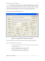
1.2.4 Green’s Function dialog box
For the green function format, the following dialog box will appear for
the insertion of the synthetic parameters required for plotting the synthetic
seismograms. This dialog box is used also for the EMPIRE tool to construct the
empirical green's function synthetics (See EMPIRE section for more detail).
Figure 7: Typical Green’s function dialog box.
These parameters are as follows:
Parameter
Description
Mechanism
Strike, Dip, Slip values and seismic
moment
Source time function
(STF)
Trapezoid : Trapezoid of T1, T2
parameters will be constructed and
Convolved with synthetics
None: No source time function will be
convolved
External : Browse to a file containing
the customized source time function
Remark
Focal mechanism: strike, dip
and slip angles in degree and
seismic moment in
dyne.cm/1020.
T1=Rise time
T2=Duration
If T2 is (0) the resulting is a
triangle pulse of T1 duration.
-External STF is a 2-column
ASCII file similar to that
constructed by test signal
tools.
Band path filter parameters
Unchecked the Filter check
Hi= Hi cut frequency
box for not using filter.
Low= Low cut frequency
Azimuth to the station in degree.
Azimuth
Number of points to skip from green’s
Nskip
____________________________________________________________________________________
Sgraph V3.7 – User Manual
Filter
27
Waveform Analysis Tools in Seismology
_________________________________________________________________________________
file.
Default = all.
Number of points to read from green’s
If Zero, the maximum of
Npoints
file.
allowed number will be read.
Components to
construct
Check Vertical, Radial or Tangential
component to construct.
Select Phases
Select/don’t select phases from the ray
file.
At least 1 component should
be checked
If checked: Gives ability to
select phases from the
predefined phases in the ray
file used in GRT.
Repeat the process with different parameters until getting accepted
result.
Sgraph supports only 99 phases per trace. In case of GRT synthetic
seismograms, this number is much exceeded. For that reason it is necessary
to select some important phases among the entire phases.
If “Select phases” is checked, the following dialog will help for this purpose
Figure 8: Typical Phase selection dialog box.
____________________________________________________________________________________
Sgraph V3.7 – User Manual
Waveform Analysis Tools in Seismology
28
_________________________________________________________________________________
In the above dialog box, all phases pre-assigned in the ray file are listed in
the “Available” box. (See appendix 3 for more detail).
To select the desired phases to be used in Sgraph do the following:
Select the phase(s) from the “Available box”(by Marking or extend
marking the desired phases).
Click the button to transfer the selected phases to the “Plotted box”
to be considered in Sgraph processes. To insert all, press “Insert all”
button. It one phase is selected, double click on the phase to select.
To remove phase(s) from the Plotted box, Mark them and click the
button. To delete all, press “Delete all” button.
See the modeling section for more detail on the usage of synthetic phases.
____________________________
1.3 Open station
Function: Open trace(s) of a specific station name and/or component from a
set of selected files from disk.
This is used to open a large number of files from successive folder in one step.
This is done by using the following dialog box.
Figure 9: Typical open station dialog box.
____________________________________________________________________________________
Sgraph V3.7 – User Manual
29
Waveform Analysis Tools in Seismology
_________________________________________________________________________________
It is considered that the data are stored into folders. Every folder corresponds to
specific event. Browse the root of the single trace data files (SAC, ASCII,
Y,..etc) from the file path box. Browse the corresponding Sum files path from
the sum file box. The sum files path consists of the summary file of all the data
The sum file name should be the same as the data folder name. Specify the
component and the station string to import. After importing all the traces, check
the info dialog box to make sure the event information are correctly imported
form the sum files.
This tool is important for the site response study by inspecting the common
station different events traces.
1.4 Delete
Function: Delete a specific trace(s) from the working window.
Insert the corresponding trace indices separated by space or coma. (Index is
written in the rightmost side of the trace) or insert (0) to delete all traces. A
confirmation dialog will ask to confirm the deletion of traces.
N.B.
After the trace deletion is confirmed, it cannot be recovered again.
After the trace deletion, the indices of the next traces will be changed. So, when
you assign traces to be deleted, delete it at once otherwise you should assign traces
again.
1.5 Info
Function: Display or change trace(s) information.
Select the desired trace using the combo given. The Information will be updated
when changing the trace index listed in the Combo box. (See the Info dialog
section for more details).
____________________________
1.6 Edit Data
Function: Edit data file using Notepad.
Open any data file using the windows Notepad to be edited or checked.
____________________________________________________________________________________
Sgraph V3.7 – User Manual
Waveform Analysis Tools in Seismology
30
_________________________________________________________________________________
Select the desired file name and edit in the opened “Notepad” window then save
the file and close “Notepad”. Notice, only Notepad is available for the data
editing in Sgraph. It is recommended to edit the large-sized files by an external
editor.
____________________________
1.7 Setup
Function: Change the Sgraph plotting setting like colors, graph options and
file naming method.
Changing is held through the following dialog:
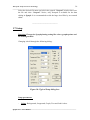
Figure 10: Typical Setup dialog box.
Setup parameters
-
Colors: Background, foreground, Graph, Text and Label colors.
____________________________________________________________________________________
Sgraph V3.7 – User Manual
31
Waveform Analysis Tools in Seismology
_________________________________________________________________________________
-
Display: Switch on/off plotting the X-grid, Y-grid lines, Info and phase
pickings.
-
File naming: File naming method in the case of multi trace saving in SAC
and ASCII formats.
When saving multiple of files in SAC or ASCII format, file names is
taken either related to index value (e.g. ***.001, ***001.SAC.. etc) or
from the trace name.(e.g. ABC.001, ABC.SAC).
Default is Name method.
The naming technique is shown in the following table.
Naming method
ASCII Formats
SAC Format
Index
Name
ABC.001, ABC.002, …etc
ABC***.001, ABC***.002, etc.
ABC001.SAC, ABC.002.SAC, …etc
ABC***.SAC, ABC***.SAC …etc.
GSE Format
ABC001-INT.GSE (for GSE INT)
ABC***-INT.GSE
ABC001-CM6.GSE (for GSE CM6)
ABC***-CM6.GSE
Where, ABC: File name inserted in the Save file dialog (constant for all files)
***: trace(s) name
001: Trace index.
Sgraph displays the new setting after closing the Setup dialog box. A
confirmation dialog box will ask for save the new setting. The setting will be
saved in an ASCII file named 'SGRAPH.SET'. Sgraph searches for this file
when start up. If not found, the default setting will be used.
N.B.:. The default and the user defined magnitude formula coefficient are saved
in this file once the magnitude tool is called.
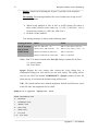
Example of a typical 'Sgraph.set' file
SGRAPH CONFIGURATION FILE
15
BACKCOLOR
7
FOREGROUND COLOR
1
GRAPHIC COLOR
12
TEXT COLOR
5
LABEL COLOR
0
Plot mode
0.20
Line width
____________________________________________________________________________________
Sgraph V3.7 – User Manual
Waveform Analysis Tools in Seismology
32
_________________________________________________________________________________
7
Symbol
2.00
Symbol size
T
X GRID LINES
T
Y GRID LINES
T
DISPLAY INFO
F
INDEX NAMING
T
PLOT PICKING
MAGNUTIDE
2
0.833000
0.000740
1.260000
ML=Log(A)+0.833Log(r)+0.00074*
0.700000
0.000400
1.400000
ML(QQ)
____________________________
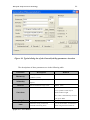
1.8 PS preferences.
Sgraph uses a facility to convert the screen plot into a Post Script file. PS
preferences dialog box receives the Post Script plotting parameters.
The plotting parameters in the PS file can be same as the Sgraph plotting
parameters defining in “Setup” (Default) or can be customized.
The following dialog defines the PS plotting parameters.
____________________________________________________________________________________
Sgraph V3.7 – User Manual
33
Waveform Analysis Tools in Seismology
_________________________________________________________________________________
Figure 11: Typical Post script properties dialog box.
The page size is only A4 in this version. Portrait and landscape modes
are allowed.
Text fonts and symbols can be chosen for a better plot. Plot mode can
be line without symbol, symbol without line or both.
Plot can be coloured or Black and white plot.
The PS file is available for a single trace, multi traces or a record section trace.
The single/multi trace PS plot can be done using the Save as PS menu
discussed below. The record section PS plot can be done using the Record
section dialog discussed later.
____________________________
1.9 Save data:
Tools for saving the current traces in different formats. For all data format,
insert the trace index to save and the output data format.
Insert a file name (without extension) in the save file dialog box. Null file is
accepted to have a full automatic file naming.
Save data formats allowed in Sgraph are as follow:
1.9.1 Save One-Column ASCII data (Sgraph 3.0
Y-format)
Function: Save the selected traces as 1-Column ASCII format
preceding by set of headers. This is a specific format of Sgraph called
“Sgraph 3.0 Y-format”. It consists of headers combining all information
related to the saved file including the phase pickings; station and event
information (See appendix 4 for the description of this format). The file can
be easily edited or plotted in other drawing software.
Traces are saved in separate files named according to the naming method
discussed in the setup section.
1.9.2 Save Two-Column ASCII data (Sgraph 3.0 XY-format)
Function: Save the selected traces as 2-Column ASCII format
preceding by set of headers. This is a specific format of Sgraph called
____________________________________________________________________________________
Sgraph V3.7 – User Manual
Waveform Analysis Tools in Seismology
34
_________________________________________________________________________________
“Sgraph 3.0 XY-format”. It consists of headers combining all information
related to the saved file including the phase pickings; station and event
information. See appendix 4 for the description of this format. The file can
be easily edited or plotted in other drawing software.
Traces will saved in separate files named according to the naming method
discussed in the setup section.
1.9.3 Save Binary SAC format
Function: Save the selected traces in Binary SAC format.
A full header SAC file will be written for the selected trace(s) including all
trace, station and event information. All information will be saved in the
corresponding header. Magnitude and Seismic moment are saved in USER0
and USER1, respectively. Phases picking are stored in the corresponding 9
SAC headers.
Traces will be saved in separate files named according to the naming
method discussed in the setup section.
N.B. Only the first 9 phases are saved, other phases will be omitted. The
focal mechanism values will be lost when saving trace in SAC format.
1.9.4 Save SAN Format (Seismic ANalysis format)
Function: Save the entire set of traces in a Binary file including all
traces information. This a special format for Sgraph in which a
compressed Binary file is constructed to combine the entire set of traces in
one file. To save a SAN file, insert the desired trace(s) to save and the SAN
file name.
The saved SAN file can be opened by the Load menu discussed above.
1.9.5 Save GSE (INT) and (CM6) format
Function: Save the selected traces as a Global Seismic Exchange (GSE)
format either uncompressed integer data (INT) or compressed (CM6)
data. Station and event information will be saved in the GSE header.
Traces are saved in separate files named according to the naming method
discussed in the setup section.
____________________________________________________________________________________
Sgraph V3.7 – User Manual
35
Waveform Analysis Tools in Seismology
_________________________________________________________________________________
N.B. Some information relating to the trace(s) being saved will be missed
when save data in this format. The GSE header can not support all the
information exists in Sgraph as a result the excess information will be lost.
1.9.6 Save WAV format
Function: Save the selected traces as a WAV audio format that can
be opened by any WAV player (i.e. Windows media player and
Real player).
The seismic traces might be resampled for a higher sampling rate before waved
as WAV file to simulate the audio frequency.
_______________________________
1.10 Save as BMP
Function: Save the working window as a Bitmap image (BMP).
This menu makes a BMP file for the traces being displayed in Sgraph window.
Insertion of the BMP file name is only required. To save a specific graph type or
trace(s) use the graph tools (e.g., redraw, Draw Spec, multitrace, etc..) before
save BMP. (See the Graph menu for details of this menu).
_______________________________
1.11 Save as PS
Function: Save the selected traces as a Post Script file (EPS).
Similar to save data formats. Sgraph makes a PS version of the selected trace(s)
in separate EPS files.
Once this menu is selected, the PS preferences dialog box will appear. Any
of the PS parameters can be changed if needed.
-
Insert the desired trace(s) index in the dialog box following the typing
rule. The saved traces will be similar to those being plotted in Sgraph
by Draw Spec menu.
____________________________________________________________________________________
Sgraph V3.7 – User Manual
Waveform Analysis Tools in Seismology
36
_________________________________________________________________________________
-
-
Insert a file name (without extension) in the Save file dialog box. The
file name will have extension “EPS”. No naming method is used in this
case.
To save a record section, use the Save PS button in the dialog box.
____________________________
1.12 Print
Function: Print the working screen to the default printer.
The desired traces can be printed during Zoom, Draw Spec, Multitrace or
Compare tools.
____________________________
1.13 Quit
Function: Quit the program.
Save your work before quitting.
_______________________________
____________________________________________________________________________________
Sgraph V3.7 – User Manual
37
Waveform Analysis Tools in Seismology
_________________________________________________________________________________
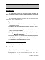
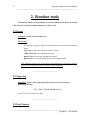
2. Routine tools
This menu consists of the principle waveform analysis tools. Refer to section
1 for the trace selection and the data entry of these tools.
2.1 Zoom
Function: Zoom in the selected trace.
How to do?
-
The mouse is using to drag and stretch the trace to the desired window
limits.
Left-Click on the trace and move mouse to drag.
CTRL+left-Click to stretch/destretch trace.
Double-Click to reset the original trace limits.
Right-Click to exit and confirm the current window limits.
N.B. Zooming routine can be applied in time domain and frequency domain
traces as well, in the last case, it uses as a type of filtering
____________________________
2.2 Tapering
Function: Apply Cosine tapering on the selected trace by using the
following function:
Y(i) = TAP - TAP*COS(PI*(i-1)/N)
Insert 'TAP' value between 0 and 1
____________________________
2.3 Fast Fourier
____________________________________________________________________________________
Sgraph V3.7 – User Manual
Waveform Analysis Tools in Seismology
38
_________________________________________________________________________________
Function: Apply Fast Fourier Transformation (FFT) on the selected trace.
Number of points used must be of integer power of 2. If not, the least closely
2n+1 value will be used.
N.B. This routine is only available for time domain traces.
____________________________
2.4 Inv. Fourier
Function: Apply the Inverse Fast Fourier Transformation (IFFT) on the
selected trace.
Convert the frequency domain trace into its corresponding time domain state.
The number of points of the new trace will be twice the number previously used
in the FFT.
N.B.
This routine is only available for Frequency domain traces
Only FFT traces produced by Sgraph can be inverted into their time domain trace.
The Inverse FFT can not recover FFT traces of the Saved San file or external FFT
traces.
____________________________
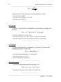
2.5 Phase Trans.
Function: Transformation of the selected trace into its Phase domain trace.
It is a simple conversion from the time domain trace into a phase domain
trace. The phase domain is transformed by using the following formula:
P( f ) e tan
1
( iY ( f ) / Y ( f ))
____________________________
____________________________________________________________________________________
Sgraph V3.7 – User Manual
39
Waveform Analysis Tools in Seismology
_________________________________________________________________________________
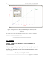
2.6 Envelop Trans
Function: Transform the selected trace into its envelop. This is done by
using the FFT transform of the selected trace after omitting the imaginary part.
The envelope Env(t) of a given trace (y(t) can be calculated as:
Env(t ) IFFT ( ABS (Y ( f ) / N / 2))
Y(f) is the frequency domain of the given trace with null imaginary part.
____________________________
2.7 Hilbert transform
Function: Do the Hilbert transform of a selected trace.
Insert the desired trace(s) index to be transformed
____________________________
2.8 Integration
Function: Integrate the selected trace using Fast Fourier Transformation.
The FFT trace is divided by the angular frequency (ω) before re-transform again
into time domain.
____________________________
2.9 Differentiation
Function: Differentiate the selected trace using Fast Fourier
Transformation. The FFT trace is multiplied by the angular frequency (ω)
before re-transform again into time domain.
____________________________
2.10 Rotation
____________________________________________________________________________________
Sgraph V3.7 – User Manual
Waveform Analysis Tools in Seismology
40
_________________________________________________________________________________
Function: Rotate the selected North and East components into Radial and
Tangential components.
The mathematical formulation of the rotation process is as follows:
R (t ) N (t ) * Cos ( ) E (t ) * Sin( )
T (t ) N (t ) * Sin( ) E (t ) * Cos ( )
Where, R(t) and T(t): the radial and tangential time series
N(t) and E(t): the north and east time series
θ: The rotation angle
How to do:
-
Insert trace(s) index of the North, East components.
The Azimuth will be extracted from the “Info” buffer. Be sure that the azimuth
value in Info is correct. If not, modify it manually.
Use “ Ignore”, “Add” or “Replace” to treat the old traces.
EX: 1,2 = (North comp is trace 1, East is trace 2)
_______________________________
2.11 Add noise
Function: Add a random noise to the selected trace.
The noise signal is proposed to be the average of three types of sine waves
with different frequencies and amplitudes (ref.). This can be represented as
follows:
Y1 = a1* rand * Sin (F1)
Y2 = a2* rand * Sin (F2)
Y3= a3* rand * Sin (F3)
For a combination of these functions with randomly weighed amplitude the
noise signal can be expressed follows:
____________________________________________________________________________________
Sgraph V3.7 – User Manual
41
Waveform Analysis Tools in Seismology
_________________________________________________________________________________
Noise = (Y1 + Y2 + Y3)/3.
The default frequencies used for F1, F2 and F3 are 10.0, 2.0, 0.1 Hz, respectively. The
amplitude of Y1 is less by 10 % from the others.
To add noise to any trace, select the appropriate frequencies and the S/N ratio. The
resulted noisy trace will be given for the acceptance.
_______________________________
2.12 Plot Mecha
Function: Plot the focal mechanism stereographic projection of a given
strike , dip and rake values.
How to do:
- Insert the strike, dip, rake values need to be plotted.
The lower hemi sphere stereographic projection plot will be shown on the
screen. The two nodal planes are given with the azimuth and plunges of the P
and T axis.
The file “Nodal.dat“ will be generated directly after plotting the mechanism plot.
To save the file as other name, type the new name in the dialog box given. The
“Nodal.dat” file can be plotted directly as a Line plot in Grapher program
(Golden Software).
The following figure is a typical Mecha plot of 45, 45 and 60, for strike, dip and
rake, respectively.
____________________________________________________________________________________
Sgraph V3.7 – User Manual
Waveform Analysis Tools in Seismology
_________________________________________________________________________________
42
Figure 12: Typical Mecha plot dialog box.
2.13 Wadati diagram
Function: Plot the Wadati diagram of the selected traces.
What is Wadati diagram?
It is a relation between the S-P time and the P arrival time. The linear regression
of this relation reveals the origin time and the (Vp/Vs) -1. The linear fitting of
this relation is done by using the SVD inversion in Sgraph tools.
How to do:
-
Select a set of traces of valid P and S phases.
The corresponding S-P vs P relation is shown to be added or ignored.
The linear regression of this plot will be automatically shown with the
resulted O.T and VP/Vs with their corresponding rms, as shown in the next
figure.
____________________________________________________________________________________
Sgraph V3.7 – User Manual
43
Waveform Analysis Tools in Seismology
_________________________________________________________________________________
Figure 12: A typical screen-shot of the Wadati diagram linear regression
dialog box.
The Wadati diagram plot can be manually inverted for the O.T and Vp/Vs parameters
by using the inversion tool as shown bellow.
____________________________
2.14 Magnitude
Function: Estimate the trace magnitude of a given trace by picking up the
maximum amplitude.
In this tool, Sgraph is able to estimate the magnitude of a given trace by navigating and
picking the maximum amplitude. The magnitude formula used in the calculation is
initially set to the ML formula used in the Egyptian National Seismic Network (ENSN),
which is as follows:
ML = Log (a) + 0.833 log (R) + 0.00074
____________________________________________________________________________________
Sgraph V3.7 – User Manual
Waveform Analysis Tools in Seismology
_________________________________________________________________________________
44
Where A is the peak to peak amplitude in meter measured from the simulated WoodAnderson record, R is epicentral distance in Km .
To accomplish this condition, the Picking process is held after the instrumental
correction and Wood Anderson simulation. This is internally done by default. The peak
to peak amplitude in this process is stored in memory and in SAN file. It is also possible
to pick the Peak to peak Wood Anderson amplitude by the Picking tool (see picking
menu). All set of amplitude picking is used later in the location process to calculate the
XMAG magnitude (See Hypoinv2000 documentation and the Location section in this
manual).
How to do :
Select the menu magnitude.
Select the trace to calculate the magnitude from (either instrumentally
corrected or not).
Follow the Amplitude picking procedure, stretch, and drag trace until a
clear view of the maximum amplitude then press R-click mouse button.
Once you got the cross cursor, press two successive L-click mouse
button for the two peaks of the maximum amplitude. Confirm the
selection by answering the given message.
The following dialog will appear:
Figure 13:Typical Magnitude estimation dialog box.
____________________________________________________________________________________
Sgraph V3.7 – User Manual
45
Waveform Analysis Tools in Seismology
_________________________________________________________________________________
The traces amplitude and the trace distance will be written in the
corresponding box. The resulted magnitude value of the default formula
will be given in the Magnitude box.
Change the magnitude formula if needed.
To retrace amplitude, press 'Amplitude' button.
To accept the resulted magnitude and store it into Info buffer, press
'Accept' button.
If it is not required to correct the instrument and/or simulate to Wood
Anderson, uncheck the corresponding boxes and retrace amplitude.
To add a new magnitude formula press 'Add' button and use the following
dialog box:
Figure 14: Typical dialog box of the new magnitude formula insertion.
Fill in the appropriate values of the new formula and write a label name of the
formula then press 'Add' button. This formula will be inserted in the magnitude
formula list of the magnitude dialog box to be used for magnitude estimation.
The new formula(s) will be saved in the 'Sgraph.set' file and will automatically
loaded with the next Sgraph execution.
____________________________
____________________________________________________________________________________
Sgraph V3.7 – User Manual
Waveform Analysis Tools in Seismology
_________________________________________________________________________________
46
3 Filter
This menu is used to apply filters to the selected traces. The filtering process
consists of two steps, one is the filter kind (i.e., low pass, high pass, etc..) . The
other is the filter type (i.e., Butterworth, Chebyshev, etc..). The user has to select
first the filter kind from the filter menu (shown below), then select the filter type
from the dialog box given.
Figure 15: A typical screen-shot of the filter type selection dialog box.
Filter types included in Sgraph are as follow:
Butterworth recursive filter
Butterworth filter (XAPIIR library)
Bessel filter (XAPIIR library)
Chebychev filter type C1 (XAPIIR library)
Chebychev filter type C2 (XAPIIR library)
Moving average filter
The XAPIIR library is the same routine used by SAC program.
In case of moving average filter type insert only odd numbers up to 11 [1,3,..11].
This filter can be specifically applied to frequency domain trace for smoothing the
spectral traces.
____________________________________________________________________________________
Sgraph V3.7 – User Manual
47
Waveform Analysis Tools in Seismology
_________________________________________________________________________________
3.1 Hipass
Function: Apply High-pass filter with any filter type on the selected
trace(s).
Select the filter type from the given dialog box and then insert the High-cut
frequency.
____________________________
3.2 Lowpass
Function: Apply Low-pass filter with any filter type on the selected trace(s).
Select the filter type from the given dialog box and then insert the Low-cut
frequency.
____________________________
3.3 Bandpass
Function: Apply Band-pass filter with any filter type on the selected
trace(s).
Select the filter type from the given dialog box and then insert the High-cut
frequency.
____________________________
3.4 PoleZero
Function: Apply a customized Pole and Zero filtering on the selected traces.
In this menu Sgraph uses the Pole and Zero values given either from a Pole-Zero
file (POZ) or from built-in or user-defined values assigned in the given response
file. The selected values will be used to construct the corresponding filter to be
convolved with the selected trace.
____________________________________________________________________________________
Sgraph V3.7 – User Manual
Waveform Analysis Tools in Seismology
_________________________________________________________________________________
48
Prepare a Pole-Zero file of the appropriate filter parameters. This tool
can be used to simulate a specific instrumental response of known Pole
and zero values or by built-In instruments.
Use the given dialog box to browse the Pole-Zero file or select a specific
instrument type.
Figure 16: Typical dialog box of the Pole and Zero filter and instrumental
correction.
The above dialog box gives the ability to use Pole-Zero values either from builtin responses or from external file or manually inserted.
- Check the POZ file box to browse a user made POZ file. See Appendix 1 for
detailed description of POZ file format.
- Check the Built-In Response to use one of the following:
Wood Anderson instrument
SS1, short period SS1 instrument.
STS2, Strekeizen2 Broad band instrument.
Trillium40
Trillium240
CMG-3T
The resulted traces are in meter.
This process is internally used in the magnitude menu by simulating the trace
into Wood Anderson instrument before the Amplitude Picking process. See the
Instrumental response section
____________________________________________________________________________________
Sgraph V3.7 – User Manual
49
Waveform Analysis Tools in Seismology
_________________________________________________________________________________
____________________________
4 Math
These routines perform mathematical operations with traces. Some
routines are single-trace processes. Others are multiple-trace processes. The
appropriate dialog box will be given for trace insertion.
In all these routines insert or select the desired trace(s) with which the
operation is to be applied. Then, follow the dialog box request for operation discussed
below. Data and/or operators should be inserted following the typing rule.
4.1 Power order
Function: Raise the amplitude of the selected trace(s) to the power “n”.
-Insert a real value “n” whose trace will be powered to. i.e. (Trace)N .
____________________________
4.2 Multiplication
Function: Multiply the amplitude of the selected trace(s) with the value
“X”.
-Insert the multiplication real value “X” whose trace will be multiplied with.
(Trace) * X
____________________________
4.3 Area under curve
Function: Calculate the area under curve for the selected trace.
-The area under curve will be hachured and the area value will be given.
____________________________________________________________________________________
Sgraph V3.7 – User Manual
Waveform Analysis Tools in Seismology
_________________________________________________________________________________
50
____________________________
4.4 Normalization
Function: Normalize the amplitude of selected trace(s).
____________________________
4.5 Absolute
Function: Absolute of the selected trace(s).
____________________________
4.6 Cumulative Sum
Function: Calculate the cumulative sum of the selected trace.
This is useful for the onset detection. It shows the abrupt changes in wave
amplitude. The mathematical formulation of the Cumulative Sum is shown in
the numerical Recipes book (Press et al., 1989).
____________________________
4.7 CrossCalc
Function: Interact with traces mathematically.
Insert the desired trace indices separated by a mathematical operator. The
accepted operators are (+,-,*,/,^). ('^' is the power).
EX: 1*2+3 = multiply trace 1 by trace 2 and add the result to trace 3.
N.B. -The trace indices and operators should be inserted without spaces or parentheses
in between.
____________________________
____________________________________________________________________________________
Sgraph V3.7 – User Manual
51
Waveform Analysis Tools in Seismology
_________________________________________________________________________________
4.8 Spectral Ratio
Function: Perform a spectral ratio operation between two frequency
domain traces. This tool is used in site correction process.
The process is performed for any frequency domain trace. The resampling
process will be conducted on the second trace to be synchronized in frequency
values.
-Insert the two trace indices separated by a space.
____________________________
4.9 Power Spectrum
Function: Perform a Power spectrum operation to a frequency domain
trace.
The power spectrum process (Pspec) between Y1,Y2 frequency traces is
expressed as follows:
Pspec (f) =
Y1 (f) . Y2 (f)
-Insert the two trace indices separated by a space.
____________________________
4.10 Cross Spectrum
Function: Perform a Cross spectrum operation between two frequency
domain traces.
The cross spectrum process (Xspec) between Y1,Y2 frequency traces is
expressed as follows:
Xspec (f) =
Y1 (f) . Y2 (f)*
Where '*' is complex conjugate
____________________________________________________________________________________
Sgraph V3.7 – User Manual
Waveform Analysis Tools in Seismology
_________________________________________________________________________________
52
-Insert the two trace indices separated by a space.
__________________________
4.11 Cross correlation
Function:
-
Calculate the cross correlation between two traces.
Insert the indices of the desired 2 traces. The Cross correlation curve and the
maximum correlation value with its corresponding lag time will be given.
________________________________
4.12 Multi Cross correlation
Function:
Calculate the Multi cross correlation of selected traces.
This process perform a successive X correlation processes between a set of
traces providing a 2-D mapping of cross-correlation coefficient and lag time. The
resulted values will be save in "MCORR.DAT" file.
-
Use the given section dialog to select the window and the indices of the
traces needed for correlation. (Don’t use a long sample of traces, this will
last a long time).
A typical example a 4 traces Multi cross correlation file is given below:
1
1
1.0000
0.0000
1
2
0.2110
0.2700
1
3
0.2222-48.5800
1
4
0.1652-51.6700
2
2
1.0000
2
3
0.2241-50.4500
2
4
0.2168-49.3700
3
3
1.0000
0.0000
0.0000
3 4
0.1928 -0.3800
4
1.0000
4
0.0000
The description of this file is a follows:
____________________________________________________________________________________
Sgraph V3.7 – User Manual
53
Waveform Analysis Tools in Seismology
_________________________________________________________________________________
First two numbers are indices of traces being correlated, third number is the maximum
X-correlation coefficient of that set, last number is the lag-time at the maximum
correlation .
____________________________
4.13 Auto correlation
Function:
Calculate the auto correlation of a selected trace.
-Select a trace to be auto correlate. The auto correlation curve will be given.
____________________________
4.14 Convolution
Function:
Convolve two selected traces.
-Insert the indices of desired 2 traces to convolve.
Result is: trace1 * trace2
____________________________
4.15 Deconvolution
Function:
Deconvolve two selected traces.
-Insert the indices of desired 2 traces to deconvolve. The second one is the
denominator.
Result is: trace1 / trace2
____________________________
4.16 Distribution
Function:
Calculate the distribution curve of a selected trace.
____________________________________________________________________________________
Sgraph V3.7 – User Manual
Waveform Analysis Tools in Seismology
_________________________________________________________________________________
54
- Select a trace to calculate the distribution.
The result is a point curve representing the recurrence of every Y value. X-axis
is the Y value. Y-axis is the recurrence or number of occurrence of this value within the
entire trace.
____________________________
4.17 Statistics
Function: Calculate some statistical parameters of a selected trace (e.g.
Mean, Standard deviation, Root mean square, number of points)
- Select a trace to calculate its statistics.
____________________________
4.18. Resampling
Function: Resample a selected trace with another sampling rate.
-
Insert the desired trace(s) index to be resampled .
Insert the new sampling rate in sample/sec.
____________________________
4.19. Calculator
Function: Open the Windows Calculator as a helping tool in waveform
analysis.
____________________________
____________________________________________________________________________________
Sgraph V3.7 – User Manual
55
Waveform Analysis Tools in Seismology
_________________________________________________________________________________
5 Correction
5.1 Instrumental
Function:
Remove the instrumental response from the selected trace(s).
Sgraph uses the user defined POZ file to deconvolve the station response from
the selected trace. (See the PoleZero filter for more detail).
Sgraph assumes that the POZ file name of the given trace is found in the Sgraph
response folder and constructed from the trace name (or station name) and the
component type as follows:
POZ file name = Tracename_comp.poz
EX:
FYM_Z.POZ
In case the POZ file is not exiting in the Response folder the Response dialog
box (See filter section) will appear for browsing a different file or use built-in
responses.
____________________________
5.2 Site correction
Function: Correction the seismic traces from a defined site effect signal.
This is done by performing the spectral ratio between the observed trace and the
Site effect trace and give the resulted trace in the time domain.
This process is internally done in the Site effect tool. Where, it corrects the
corresponding observed traces from the resulted Site effect (see Site Effect section for
detail).
5.3 Remove DC
____________________________________________________________________________________
Sgraph V3.7 – User Manual
Waveform Analysis Tools in Seismology
_________________________________________________________________________________
Function:
56
Remove the DC trend from the selected trace(s).
____________________________
5.4 Remove O.T.
Function:
Remove the Origin time from the arrival time trace(s).
The arrival time trace is subtracted from the origin time to produce the travel
time trace.
The origin time stored in buffer will be used in this process, if no origin time is
stored the program prompt of it.
N.B. Make sure to insert the correct O.T. value before proceeding.
____________________________
5.5 Reduce T.T
Function:
-
Reduce the selected trace(s) by the ratio (distance/velocity).
Insert trace(s) index to be reduced,
Insert the reduced velocity.
The distance of the selected traces will be extracted from the “Info” buffer. Be
sure that the distance values in Info are correct. If not, modify it manually.
____________________________
____________________________________________________________________________________
Sgraph V3.7 – User Manual
57
Waveform Analysis Tools in Seismology
_________________________________________________________________________________
6 Test Signal
Function:
Construct several types of signals for data analysis and testing.
The data in these tools are inserted through the following test signal dialog.
Figure 17: Typical dialog box of the Test wave generation.
Fill in the trace parameters (number of points and sampling rate) of the resulted
signal and follow the dialog request for each signal.
6.1 Line
Construct a line function of amplitude (A):
Y(t) = A.
- Insert the amplitude “A” of the function.
____________________________
6.2 Spike
____________________________________________________________________________________
Sgraph V3.7 – User Manual
Waveform Analysis Tools in Seismology
_________________________________________________________________________________
58
Construct a Spike of amplitude A and position T:
Y(t) = 0 at [t ≠ T]
and
Y(t) = A
at
[ t = T].
- Insert the amplitude (A)
- Insert the spike position in the trace (T) in sec.
(Times should be within the trace limits)
____________________________
6.3 Step Function
To construct a step function of Amplitude (A) and duration T1+T2:
Y(t) = 0
at [T1 >t > T2] and Y(t) = A at [T1 < t < T2].
- Insert the amplitude (A)
- Insert the Starting time of step (T1) in sec.
- Insert the Ending time of step (T2) in sec.
(Times should be within the trace limits)
____________________________
6.4 Sine/Cosine wave
Construct a Sine wave trace of amplitude (A), Frequency (F) and Phase (P):
Y(t) = A* Sin ( 2 π Ft +P)
- Insert the amplitude (A) of Sin wave
- Insert the Frequency (F) in Hz.
- Insert the Phase (P) in Deg.
____________________________
6.5 Brune disp/vel
Construct a simulation of Brune function for displacement and velocity
spectra. For a flat part (Ωo) and Corner frequency (fc) the Brune model
displacement is expressed as :
____________________________________________________________________________________
Sgraph V3.7 – User Manual
59
Waveform Analysis Tools in Seismology
_________________________________________________________________________________
Y( f )
o
1 ( fcf ) s
Brune model for velocity is the same function multiplied by 2*PI*F
- Insert the Flat part (Ωo)
- Insert the Corner Frequency (fc) in Hz
- Insert the slope fall off (s).
____________________________
6.6 Sweep
Construct a Sweep function of amplitude (A) and frequency ranging from
F1 to F2.
Y (t) = A * Sin (2 π F),
F= [F1:F2]
- Insert the amplitude (A) of Sine wave
- Insert the Frequency (F1) in Hz., the lower frequency of the signal.
- Insert the Frequency (F2) in Hz., the higher frequency of the signal.
____________________________
6.7 Mixed
Construct Sinusoidal wave of amplitude (A), Frequency (F) mixed with
attenuation operator of power (P).
Y (t ) ASin(2Ft ).e Pt
- Insert the maximum amplitude (A) of the signal.
- Insert the Frequency (F) in Hz.
- Insert the attenuation operator (P).
____________________________
6.8 Polynomial
Construct a polynomial function of the degree “3”.
Y(t) = a0 + a1t + a2t2 + a3t 3
- Insert the coefficients: a0 (A), a1(B), a2 (C) and a3 (D).
____________________________
____________________________________________________________________________________
Sgraph V3.7 – User Manual
Waveform Analysis Tools in Seismology
_________________________________________________________________________________
60
6.9 Trapezoid
Construct a trapezoid with Rise time (T1) and
Duration T2
- Insert the trapezoid rise time (T1) in sec
- Insert the trapezoid duration (T2) in sec.
T1
T2
N.B. A triangular function can be constructed by inserting the value T2=0.
____________________________
6.10 Noise Signal
Construct a randomized noise signal as proposed in the Add noise section.
- Insert the S/N ratio (relative to 1)
- Insert F1, F2, F3 frequencies in Hz.
____________________________
____________________________________________________________________________________
Sgraph V3.7 – User Manual
61
Waveform Analysis Tools in Seismology
_________________________________________________________________________________
7 Inversion
Function: Apply matrix inversion tools on the selected trace with respect to
built-in functions.
Sgraph makes the mathematical regression between selected trace(s) and a
selected function and plot the best-fit curve with the solved parameters and errors. For
more information of the inversion tools refer to Press et al. (1989).
The inversion is either linear type (SVD) for polynomial, arrival time fitting and
Wadati diagram fitting; or nonlinear inversion type (Marquard) for the Brune
displacement and Brune velocity models. Inversion for Q-Freq relation, PGV-Dist
relation, and MLTW are also provided. Because the requirements of the last three
relations are not able to be extracted from the working traces, those are either
implemented internally or from individual menu.
The next table shows the available functions for the SVD and Marquard inversions.
Inversion tool Function name
Polynomial
Linear
inversion
(SVD)
Arrival time vs
distance
Wadati diagram
Formula
Unknown parameters
2
a0 + a1*X + a2*X + …an*X
n
A0, a1,a2, … an
T t 0 t (V=slowness)
Origin time, Vp
S-P time = a0 + a1*T
Origin time, Vp/Vs
(T = arrival time)
Nonlinear
inversion
(Marquard)
Brune model
Y( f )
displacement
Brune model
o
1 ( fcf ) s
o * 2 * PI * f
1 ( fcf ) s
Y( f )
velocity
n
Q vs Freq
Q = Qo f
Genetic
Algorithm
MLTW
Energy function (see MLTW
Genetic
Algorithm
PGV-Dist
Flat part, corner
frequency
Flat part, corner
frequency
Qo, n
See MLTW section
section)
Peak ground velocity- distance
C1, C2 C3, and C4 coefficients
relation.
representing, amplitude scaling,
Magnitude scaling, geometrical
____________________________________________________________________________________
Sgraph V3.7 – User Manual
Waveform Analysis Tools in Seismology
_________________________________________________________________________________
62
spreading and anelastic attenuation,
respectively.
7.1 Linear fit (SVD)
Linear inversion using Singular Value Decomposition. Available functions
are:
The polynomial function, Arrival time function and Wadati plot.
Polynomial function:
Polynomial function of n orders. This is internally used to solve the linear
fitting problems (i.e. polynomial of order 1). As a tool it can be used for the
linear regression of any dataset.
Arrival time vs distance relation:
T t 0 t
Where,
T: is the phase arrival time
to: Origin time
△: epicentral distance
t : slowness of the phase.
This is an application of the one-order polynomial fitting for the
slowness (t) and the origin time (t0) of the selected traces. According to the
behaviour of the arrival times with distance, the best-fit curve reveals the
appropriate apparent velocity (1/t) and the origin time.
How to fit the arrival time curve for a set of traces.
-
Select the SVD tool from inversion menu.
-
Insert trace indices of to be used in inversion. Each trace must have at least
one phase picked.
____________________________________________________________________________________
Sgraph V3.7 – User Manual
63
Waveform Analysis Tools in Seismology
_________________________________________________________________________________
-
From the given dialog box (Record section dialog box) select the respected
phase to be used in inversion from the onset phase list box.
Select the function “Travel time fitting” from the inversion functions dialog
box.
If the inversion succeeded, the picking and the fitted curves with their
corresponding standard error will be given.
Repeat the inversion for different traces and functions if required.
Figure 18: A typical example of the linear regression of Pg arrivals. Blue curve
is Pg arrival times versus epicentral distance. Green is the corresponding best
fit curve. Internal dialog box shows the resulted values of to and t.
Wadati diagram: S-P time = a0 + a1*T
Another application of the one-order polynomial fitting where the relation
between the S-P time vs P arrival reveals the Vp/Vs value and the origin
time.
How to fit the Wadati diagram plot:
____________________________________________________________________________________
Sgraph V3.7 – User Manual
Waveform Analysis Tools in Seismology
_________________________________________________________________________________
64
The Wadati plot is automatically constructed and fitted by using the Wadati
plot menu (see above).
For a previously constructed Wadati plot, a fitting can be done by the next steps:
-
Select the SVD tool from inversion menu.
Insert trace index of the previously constructed Wadati plot
Select the function “Wadati plot function” from the given dialog box.
If the inversion succeeded, the observed points (Open circles) and the best-fit
line will be shown. The resulted Vp/Vs and origin time with their
corresponding errors will be shown in the giving dialog box. The resulted
line can be added to the Sgraph traces (if desired). See the Wadati plot menu
(above) for a typical screenshot of the Wadati plot fitting.
____________________________
7.2 Nonlinear fit (Marquard)
None-linear inversion using Marquard method.
The available functions are the following:
-
Brune1 for Displacement (see the above table),
Brune1 for Velocity (see the above table).
Brune2 for Displacement (under construction)
Brune2 for Velocity (under construction)
PGV-dist relation (see text below)
How to fit a spectral trace with Brune model
-
Select the nonlinear fit menu for inversion.
Select the suitable trace to fit
From the given dialog box select the function corresponding to the selected
trace for inversion (e.g. Brune displacement or Brune velocity).
If the inversion succeeded, the resulted fitted line and solved parameters will
be shown with the corresponding standard errors.
Repeat the inversion for different traces and functions if required.
Resulted curve can be added as a new trace to the Sgraph list.
Next Figure shows typical inversion of Brune displacement spectral fitting.
____________________________________________________________________________________
Sgraph V3.7 – User Manual
65
Waveform Analysis Tools in Seismology
_________________________________________________________________________________
Figure 19: A typical example of the nonlinear inversion of Brune model
displacement function. Blue curve is observed FFT trace, green curve is the
corresponding best fit curve. Internal dialog box shows the resulted values of
Flat part and corner frequency.
Source Parameters estimation:
According to the calculated spectral parameters, the earthquake source parameters are
automatically estimated. The seismic moment (Mo) is directly estimated form the
solved Flat part by using the Keilis-Borok (1959) relationship:
Mo 4v 3 R FUo
Where, ρ is the density of the medium, R is the epicentral distance, v is the P-wave
velocity, F is the free surface factor (assumed as 2), and Uθφ is the mean radiation
pattern (0.55). Accordingly, moment magnitude (Mw) is estimated by using Kanamori
(1977) relationship:
____________________________________________________________________________________
Sgraph V3.7 – User Manual
Waveform Analysis Tools in Seismology
_________________________________________________________________________________
M w log(
66
Mo
) 10.73
1.5
The source radius (r) and stress drop (∆σ) are estimated following Madariaga (1976):
r 0.32 Vpf c
7 Mo
16r 3
Next figure shows typical dialog box of the earthquake source parameters estimation of
the previous spectral fitting.
Figure 20: A typical example of source parameters estimation dialog box.
The above dialog box consists of all the parameters required for the source parameters
estimation. The fitted spectral parameters are inserted in place. It is important to change
the unit of the flat part (m.sec or cm.sec) that corresponds to the windows used if
required. This is to keep the resulted seismic moment in dyne.cm. The wave velocity
and density are required parameters for the Keilis-Borok equation. Insert the appropriate
wave velocity and density according to the window selected. Moreover, the anelastic
attenuation box is used to correct the spectra from attenuation. Insert the appropriate
value if desired. Use 'update' button to update the calculation. Use 'Repeat' button to
____________________________________________________________________________________
Sgraph V3.7 – User Manual
67
Waveform Analysis Tools in Seismology
_________________________________________________________________________________
repeat the spectral fitting. Use 'Save to disk' button to save the resulted parameters in an
external file.
___________________________
7.3 PGV-Dist relation : (Peak ground velocity- distance relation)
This tool implements a nonlinear inversion for PGV values measured from a
range of distance for a given earthquake magnitude value. A maximum distance points
can be used up to 999 points and number of magnitude values is up to 99. An example
of a pre-defined PGV-distance relation file in which the PGV is given for a number
distance points and different magnitude values is shown in Appendix 9.
The PGV attenuation relation with distance R for a given magnitude (M) is
given by:
Ln (PGV) = C1+ C2*M + C3* LOG (R) + C4*R
Where, C1, C2, C3 and C4 represent the Scaling coefficient, Magnitude
coefficient, Geometrical spreading and anelastic attenuation, respectively.
Simply, Sgraph searches for the values of those coefficients that best-fit the
observed PGV values by Genetic Algorithm.
How to do ?
-Use the PGV-Dist menu to browse for the pre-defined PGV-Dist file.
-The respected values of the PGVs with different magnitudes will be plotted
and a genetic dialog box will be prompted.
- Enter the appropriate searching parameters.
- The searching procedure will start and the plot will update when best fit
increase.
- The observed, best-fit-data and the resulted coefficient will be saved in the
file "PGV-Dist_res.dat".
___________________________
____________________________________________________________________________________
Sgraph V3.7 – User Manual
Waveform Analysis Tools in Seismology
_________________________________________________________________________________
68
8 PhaseID
Tools for phase identifications using travel time table or synthetic data.
These tools use 2 types of phase data sources and 2 types of phase identification
modes. This makes it easy to identify phases from observed or synthetic traces. The
2 modes of identifications maintain the user to either search about the phase
corresponding to the selected wavelet (Search mode) or insert a specific phase to
know its corresponding wavelet (Insert mode).
Phase data sources:
1-Green function file:
This is the output file given from the GRT Algorithm (see Appendix 3). It
consists of all the information needed to extract phases used in generating the
synthetic seismograms.
-Insert the origin time of the selected trace to fit with the travel time of phases.
2-Travel time table:
This is a user supply Travel Time Table. It gives the different phase names and
their travel times for the given distances.
-Insert the Origin time and distance to extract data from table. (See Appendix 2
for more information)
8.1 Search Phase
Function: Identify the phase name and type of a specific wavelet.
How to do?
-Select the desired trace to use.
- Do the required adjustment in the trace using the given navigation tools (see
Navigation for more details). If none, press No
-Select the source of phases, either from “LOADED TABLE” or “ASERIESO”.
____________________________________________________________________________________
Sgraph V3.7 – User Manual
69
Waveform Analysis Tools in Seismology
_________________________________________________________________________________
If “LOADED TABLE”:
Insert the origin time and distance to extract phases from table. (If there
is no table in memory, you will be asked to load a table).
If “ASERIESO”:
Select the Green function file name.
Insert the suitable origin time to match the arrival times of the plotted
trace.
If phases are successfully retrieved from the above two sources, do the following:
Left Click over the plotted trace on the desired place will insert the
closest phases to this position.
Left Click again will remove the plotted phases in this position.
Right Click to return.
N.B. once the desired phases are plotted. The phases will be stored in memory for
further use.
____________________________
8.2 Insert Phase
Function: Insert a specific phase name over the plotted trace in its exact
arrival time.
How to do?
Select the desired trace to use.
Do the required adjustment in the trace using the given navigation tools
(navigation for more details). If none, press “No”
Select the source of phases, either from “LOADED TABLE” or
“ASERIESO”.
If “LOADED TABLE”:
Insert the origin time and distance to extract phases from table. (If there
is no table in memory, you will be asked to load a table).
If “ASERIESO”:
Select the corresponding green function file.
Insert the suitable origin time to match the arrival times of the plotted
trace.
____________________________________________________________________________________
Sgraph V3.7 – User Manual
Waveform Analysis Tools in Seismology
_________________________________________________________________________________
70
If phases are successfully retrieved from the above two sources, the Insert phase
dialog box will appear as follows:
Figure 21: A typical screenshot of phase identification dialog box.
The Phase identification dialog box consists of two list boxes.
A right-side box listing all the available phases found in table or in green
file; and a left-side box listing the plotted phases.
Double-Click on the desired phase from the right-side list box to be
inserted and plotted at the corresponding position overlaying the trace.
Double-Click on the desired phase from the left-side list box to be
removed from the plot.
OK to return.
The following figure shows a typical example of Sgraph phase
identification routine.
____________________________________________________________________________________
Sgraph V3.7 – User Manual
71
Waveform Analysis Tools in Seismology
_________________________________________________________________________________
Figure 22: A typical example of the Phase identification routine. In this screen,
the phase(s) selected in the dialog box will be plotted in its corresponding time
in the trace.
____________________________
8.3 Compare Phase
Function: Compare a given set of phases with different traces.
This routine is almost the same as “Compare” tool, but instead of using 2 traces,
we use one trace and a set of phases.
How to do:
Follow the same way as “Compare” for selecting trace 1.
Insert the source of phases (either “TABLE” or “ASERIESO”).
____________________________________________________________________________________
Sgraph V3.7 – User Manual
Waveform Analysis Tools in Seismology
_________________________________________________________________________________
72
The phases which are already selected in the “Insert phase” or “Search phase”
modes or which are flagged in the RID file will be plotted over the trace at their
corresponding arrival times. (Be careful to insert a suitable origin time).
- To drag phases over the plotted trace, follow the same procedures of
“Compare” in the graph menu.
The next figure shows a typical example of Sgraph compare phase routine.
Figure 23: A typical example of the Compare phase routine. In this screen, the
nominated phases (in red) can be moved forward/backward over the trace in
use as a way to observe the most represented phases in waveform.
N.B. If the travel times of phases are not suitable with the plotted trace, there might be
phases appeared for the first while that because phases are either located after or
before the window limits. Drag phases backward or forward until find the phases.
____________________________
8.4 Save Phases
Function: Save the selected phases of either the Search or insert mode.
____________________________________________________________________________________
Sgraph V3.7 – User Manual
73
Waveform Analysis Tools in Seismology
_________________________________________________________________________________
N.B. The saved phases produced by Sgraph cannot be used in Phase ID tools for this
version.
____________________________
8.5 Load Table
Function: Load a user supply travel time table to be used in the Phase
Identification and comparison tools.
-Insert the filename of travel time table. See Appendix 2 for the table format
Once the table is loaded it will be available as long as Sgraph is running.
____________________________
____________________________________________________________________________________
Sgraph V3.7 – User Manual
Waveform Analysis Tools in Seismology
_________________________________________________________________________________
74
9 Picking
Here are comprehensive tools for picking phases either manually or
automatically. Modification and deletion of phases are provided similarly. The
amplitude picking is also provided. Sgraph has the ability to support 99 phases per
trace. Each phase is stored in a string consisting of the Phase name, Phase polarity,
Phase weight and Phase time. The string takes the following form:
Pg_D0_12345.00
Where:
Pg
: Phase name
D
: Polarity D or U
0
: Weight: 0-3
12345.00: Phase time in sec. Relative to the starting time of the trace.
This string is automatically constructed after phase picking and is shown in the Info
dialog in the picking box.
To pick phases or amplitude from the given traces, the Picking dialog box is given, as
shown below:
Figure 24: Typical PhasePicking dialog box.
____________________________________________________________________________________
Sgraph V3.7 – User Manual
75
Waveform Analysis Tools in Seismology
_________________________________________________________________________________
In the next menu, the functionality of this dialog box will be explained in
detail.
____________________________
9.1 Pick/Del Phases
Function: Picking or deleting phases.
The above dialog will be given once this menu is selected. By using this
dialog, you can run over the entire Sgraph traces (the time domain traces
only) and pick, modify, delete any phase.
Change trace:
Once the Picking dialog appears, watch the Trace# value. This shows the
current trace in process.
To change the trace under process
Use: |< First : Jump to the 1st trace in sequence
>| Last: Jump to last trace in sequence.
<< Prev: Go to the previous trace
>> Next: Go to next trace.
Pick phase automatically:
Press “Auto pick”:
The auto pick routine is applied on the current trace. If pick succeed, the resulted
picking will be added automatically to the current phases having a name of “Pa” (auto
pick). The polarity is given “?” and weight is given “3” because auto pick can not
calculate them. Modify them by using the “Modify Pick” button, see below.
Pick phase manually:
Press Manual picking.
____________________________________________________________________________________
Sgraph V3.7 – User Manual
Waveform Analysis Tools in Seismology
_________________________________________________________________________________
76
o Follow the zoom tool to stretch and adjust the trace until the phase
appears clearly in an appropriate window than press Right-Click mouse.
o When the cursor appears as a cross, put the cursor over the exact time of
phase and Left-click mouse.
o Insert/select the phase name, polarity, and weight, in the phase dialog
box given below then press Accept. The phase string is constructed and
added as a new phase belongs to the trace under processing.
Figure 25: Typical example of phase information insertion dialog box.
o After phase acceptance, the trace window will show again to pick
another phase if needed.
o To finish picking in that trace Right-Click mouse twice.
o Make sure that the phase is inserted in the picking dialog “Phase exist
“ box.
Modify Phase:
Select (Highlight) a Phase to modify from the “phase exists“ box and press
“Modify Pick” button.
A picking process will start giving a cross cursor to pick a phase. If you
don’t need to change phase time, Right-Click mouse.
The phase dialog will appear to modify its contents. Phase name, Polarity
or weight.
N.B.: Select only one phase at a time to be modified, if multiple phases are
selected; only the first will be used.
Delete Phase(s):
____________________________________________________________________________________
Sgraph V3.7 – User Manual
77
Waveform Analysis Tools in Seismology
_________________________________________________________________________________
Select (Highlighted) phase(s) to be deleted from the “Phase exists “ box
and press “Delete Phase” button. Multi-selection is accepted.
A confirmation dialog will ask to confirm the deletion. Press yes if you are
sure to delete (NO UNDO FOR THIS PROCESS).
Assign Phases:
In the case of picking a phase from traces belong to same station (e.g. three
components), it is convenient to assign the picking from one trace to others. In
other words, instead of pick the P-phase from every trace individually, we can
pick only one trace and assign the same phase time and name to other traces.
This can be done by “Assign phase”.
Select (Highlight) the phase to be associated to other traces.
Press “Assign phase”.
Select a trace from the given box to be assigned with the same phase.
Watch the trace information shown in the dialog to make sure of the trace
being assigned.
Repeat the process of any other trace having the same condition.
Amplitude picking:
To pick the Peak to Peak amplitude for the given trace, use the 'Pick amplitude'
button. Once the 'Pick amplitude' button is pressed the current trace will be corrected
instrumentally and simulated to Wood Anderson seismogram. During the instrumental
correction process, Sgraph searches for the default file name of the POZ file for the
current trace. In case the file does not exist, the response dialog box will be prompted
for the response parameters (see response correction section).
After this point, the picking navigation tool will be executed to enable the adjustment of
waveform to get a clear view of the maximum waveform amplitude.
Move/stretch trace for the maximum amplitude, then right-click mouse.
Press two successive left-click muse button at the minimum and maximum phase
amplitude.
The picking amplitude values of the entire traces will be stored in memory and will be
stored in SAN files.
____________________________________________________________________________________
Sgraph V3.7 – User Manual
Waveform Analysis Tools in Seismology
_________________________________________________________________________________
78
N.B. – The assign phase will be added to the new trace as a new phase with same time,
name, polarity and weight.
____________________________
9.2 Auto Picking
Function: Apply auto picking tool to specific trace(s).
Insert the index of trace(s) desired to be auto picked.
The auto picking routine will run assigning auto pick phase (Pa) for every trace
(if succeed). If not succeed, Sgraph gives warn.
In the case when the “Pa” phase coincides with a pre-existing phase, a request
will appear to confirm the replacement or ignorance of the new picking.
____________________________
9.3 S-Pick Calc.
Function: Calculate the S-phase arrival time from a predefined P-phase by
using the VP/Vs relation and Origin time. (VP/Vs = Sqrt (3) as fixed value)
This tool provides a rough estimation of S-wave arrival only for the purpose of
windowing. It is not accurate enough to be used for location or the travel time
estimation. Make sure to revise this picking by using the Picking tools for more S-wave
precision.
9.4 Assigning Phases
Function: Assign a set of phases to a specific trace.
Insert the indices of the source and target traces.
Source trace: trace from which the phases are used.
Target trace: trace to which the phases will be assigned.
____________________________________________________________________________________
Sgraph V3.7 – User Manual
79
Waveform Analysis Tools in Seismology
_________________________________________________________________________________
____________________________
9.5 MCCC
Function: Perform Multi-Channel Cross Correlation technique (VanDecar
and Crosson, 1990).
The idea is to invert a manually picked data set in a least square sense to obtain
a new set of picking depending on the cross correlation between the entire set of
traces. See VanDecar and Crosson (1990) for more detail.
It is required to assign a correlation window parameters within which the
correlation will be performed and some other parameters to control the MCCC
process. These are done using the following dialog box.
Figure 26: Typical MCCC setting dialog box.
The dialog box content is described as follows:
Phase: The phase index to be used. Phase 1 is the only permitted phase
in this version.
Win-len: whole correlated window length in sec
Onset-len: Onset time duration.
Tapering len: Tapering window length.
____________________________________________________________________________________
Sgraph V3.7 – User Manual
Waveform Analysis Tools in Seismology
_________________________________________________________________________________
80
Int. srate: Sampling rate of data to be used in resampling.
Attenuation: Attenuation value
BP filter: Band pass Chebyshev filter values if the “Apply filter” box is
checked.
Shifts: Levels of coarseness in the search
shift1, shift2, shift3: Shifting values in sec for level1, level2 and
level3.
Default P and S button are used for the default values for either P or S
wave picking.
After inserting the appropriate values, the selected traces will be aligned and plotted
according the inserted parameters. The typical MCCC window is shown below.
Figure 27: A typical screen-shot the MCCC windowing routine.
If the window parameters are not preferable, press “NO” to return to the window
parameter dialog.
____________________________________________________________________________________
Sgraph V3.7 – User Manual
81
Waveform Analysis Tools in Seismology
_________________________________________________________________________________
If acceptable, press “YES”, the following dialog will appear.
Figure 28: Typical MCCC Result dialog box.
This is a typical “MCCC Result” dialog box. The MCCC result is plotted in a record
section plot of Equi-distant type.
The purpose of this dialog is to show the MCCC result with a convenient way.
It is important to notice that the trace indices needed here is not the actual trace
indices but the trace number in the order of selection. I mean the first selected trace will
have index1 and so on.
How to see results:
-
-
Insert the trace(s) indices to be shown, [0] to show all.
Insert data limits to focus for a specific part of the trace. Or press “Mouse
selection” button for mouse selection tools.
The Scaling factor, Normalization and Relative X-axis are the same as in
Record Section Dialog.
The correlated window of the traces will be plotted in the equidistant section
overlaying by the original picking noted as “P0” and the MCCC picking
noted as ”P1”.
Press “Update” to Update/Draw the selected parameters.
After visual checking of the whole set of traces observing the original (P0)
and the final picking (P1), confirming that the MCCC improved the picking
go to the next step.
____________________________________________________________________________________
Sgraph V3.7 – User Manual
Waveform Analysis Tools in Seismology
_________________________________________________________________________________
-
82
Press “Confirm” button to open the “Confirm Dialog” as follows.
Figure 29: Typical MCCC confirm result dialog box.
The description of the list box content of this dialog is as follows
[Trace index] [Original picking] [MCCC picking] [Residual] [Trace name].
N.B. The residual above is the standard deviation of the residuals associated with the
corresponding trace. (Equation 8, page 158, VanDecar and Crosson, 1990).
-
How to confirm picking:
Mark on the trace(s) lines needed to be confirmed.
Confirm the picking by pressing “Confirm” button. This will replace the original
picking with the new one.
Press “Reject” to exit without confirmation. This will keep the original picking as it
is.
Press “Return” to go back to the “MCCC Result” dialog box to show another set of
traces.
Once “Confirm” Button is pressed, the MCCC picking and either replace the original
picking or added as new pickings. Follow the given dialog for the appropriate usage of
the MCCC picking.
For the non-marked lines, the picking value will be rejected.
____________________________________________________________________________________
Sgraph V3.7 – User Manual
83
Waveform Analysis Tools in Seismology
_________________________________________________________________________________
____________________________
9.6 Delete Picking
Function: Delete the entire set of phases from a selected trace(s) at once.
The process is a faster way than the delete phase in the Picking dialog. It is used to
delete all phases from a set of traces.
Insert the desired trace(s) to delete phases from.
A confirmation dialog will ask to confirm the deletion. Press yes if you are
sure to delete (NO UNDO FOR THIS PROCESS).
____________________________
9.7 Load Picking
Function: Load picking previously saved by Sgraph.
-Select the File name saved by Sgraph.
Once loaded the picking values will be shown in the plotting traces and in “Info”
____________________________
9.8 Load SAC Picking
Function: Load data picking previously saved by SAC. The SAC picking
file is the Standard file id “B” form. (See SAC document for more detail)
- Select the File name saved by SAC.
Once loaded the picking values will be shown in the plotting traces and in “Info”
____________________________
9.9 Save Picking
____________________________________________________________________________________
Sgraph V3.7 – User Manual
Waveform Analysis Tools in Seismology
_________________________________________________________________________________
84
Function: Save the current picking.
The entire phases existing in Sgraph will be saved in "DAT" format of comma
separator. The format preserves all the information of the station location and the
phase’s arrival time, polarity and weight. The file is tabulated in a rows and column.
Each row is a set of one trace phases. Columns are in sequence:
Index, station name, long, lat, phase1, phase2, phase3 ,etc…
The phases are sorted in the order of arrival in the first trace. Phases that
doesn’t exist in a given trace(s) are replaces by a Null values. See Appendix 8.
____________________________
____________________________________________________________________________________
Sgraph V3.7 – User Manual
85
Waveform Analysis Tools in Seismology
_________________________________________________________________________________
10 Synthetic
This section explains tools for generating synthetic seismograms using different
techniques and performing 1-D waveform modelling.
The available techniques in this Sgraph version are:
The Generalized Ray Theory (GRT) (Helmberger, 1974, 1983)
Discrete Wave Number (DWN) (Bouchon, 1981)
10.1 GRT (Generalized Ray Theory)
Function: Construct synthetic seismograms for a given velocity model and
ray types using the Generalized Ray Theory (GRT). See Helmberger (1974, 1983)
for detail.
How to do?
To construct a successful synthetic seismogram the following are needed:
Model file:
This is the velocity model of the media in “MODEL” format (See Appendix 3 for
detail).
Ray file:
This is file consisting of the specific rays to be generalized in synthetic
seismograms. This should be in “RAY” format (see Appendix 3).
Fill in the GRT dialog (shown below) with the required parameters to generate
the Green’s function and ASERIESO files.
____________________________________________________________________________________
Sgraph V3.7 – User Manual
Waveform Analysis Tools in Seismology
_________________________________________________________________________________
86
Figure 30: Typical dialog box of the Generalized Ray parameters insertion.
The descriptions of these parameters are in the following table.
Parameter
Distance(s)
Azimuth(s)
Interval
Description
Set of epicentral distance of
Remark
Default: 100 km
synthetics (in km).
Set of Azimuth for synthetics (in
Default: 50 km
Degree)
Interval of distance range in km
Default: 10 km
Start time of the synthetic (in sec)
= Distance /7
If not, synthetic record may be
Start time
outside window length.
-This value is automatically selected
when press Auto
Sampling Rate
Auto
Sampling rate of synthetics
Default : 20 SPS
Automatic setting of distances
Press to do automatic set of distance
Azimuth and starting times.
values using the inserted interval
____________________________________________________________________________________
Sgraph V3.7 – User Manual
87
Waveform Analysis Tools in Seismology
_________________________________________________________________________________
value. The starting time is selected
automatically.
Model file name
Ray file name
Model file name in “MODEL”
Velocity model, control parameters
format
of GRT (See appendices for detail).
Ray file name in “RAY” format
Ray segments to be used in GRT.
(See appendices for detail)
Output name of the green’s function
This is the base of the Green’s
file.
function file. The distance value will
be attached to this name for synthetic.
Green’s file name
This can be opened directly using
Open menu to construct synthetic
seismograms.
Fill in the distance box with the desired distances (using the typing rule). For
range of distance use ‘:’ between the 2 distance range. Make sure to insert a
suitable interval value in the interval box. Press ‘Auto’ button to set the
required distance. See the total trace box to verify the number of traces in the
accepted range. The Azimuth values will be constant in all distances as default,
modify it if required.
Check the GRT arguments checkboxes for the suitable case.
Press “START” to start GRT.
The “Message” box displays the progress result of the GRT technique. For every
distance range a green’s function file will be constructed having a name proceed by
‘_’ and the equivalent distance. The progress bar shows the progress rate for every
file.
If the GRT progress is successfully finished, press “Synthetic” button to open
the green’s function dialog box needed to construct the synthetic seismograms.
Fill in the green‘s function dialog (see green function section) to construct the
synthetic seismogram.
____________________________
10.2 Wave Number (Discrete Wave Number method):
(This tool under development)
____________________________________________________________________________________
Sgraph V3.7 – User Manual
Waveform Analysis Tools in Seismology
_________________________________________________________________________________
88
This tool employs the Discrete Wave Number method (Bouchon, 1981) and the
method of reflectivity and transmissivity matrices of Kennett (Muller, 1988) to
construct synthetic seismograms of a specific model and distance ranges. This code is
compiled from the Seisan package (Jen, 1992) after appropriate modifications.
This is done by using the following dialog box.
Figure 31: A typical Bouchon parameters dialog box.
The above dialog consists of all the requirements to perform a DWN seismogram.
How to do DWN synthetic seismograms:
o Fill in the Distance, azimuth, focal mechanism, Source time function
(STF), filter value, etc...
o Specify, sampling rate, number of points, depth.
o Browse/insert model file (as in Appendix 7).
o Browse/insert output file (green's function file).
____________________________________________________________________________________
Sgraph V3.7 – User Manual
89
Waveform Analysis Tools in Seismology
_________________________________________________________________________________
o To synthesize specific trace(s) that are loaded in Sgraph, insert their
indices and press "Get Dist/Azim" to retrieve their corresponding
distance and azimuth.
o To synthesize a specific distance range, fill in the box (no need to fill the
trace index in this case).
o Specify the trace type (displacement, velocity, acceleration) and
components to construct (Vertical, Radial, Tangential).
o To construct synthetic seismograms press "OK". Sgraph constructs the
specified Synthetic seismograms from the output file and consider them
as new traces in Sgraph.
For more information related to DWN refer to Bouchon (1981).
____________________________
10.3 Modeling:
Function: Perform a complete waveform modelling tools by using genetic
algorithm.
Here is powerful tools for matching the observed and synthetic seismograms and
solve the different parameters of 1-D velocity model and focal mechanism corresponds
to a set of observed seismograms. Abdelwahed (2006); and Abdelwahed and Zhao
(2005) 2006) develop this technique originally for a single 3-component station by
using a manual iterative technique to estimate the velocity structure beneath southwest
Japan. In this version of Sgraph, the technique is provided after being improved to be
applied on multiple of stations and to search the modelling parameters automatically by
the micro-genetic algorithm. This makes the waveform modeling process faster and
more stable.
The idea of performing the waveform modelling is to compare the synthetic
seismograms constructed by using the GRT technique with the corresponding observed
seismograms. The genetic algorithm is employed to handle the search over the entire
velocity model or focal mechanism parameters. The genetic search is guided by the
maximum cross correlation coefficient between the observed and synthetic traces. The
micro-genetic (micro-GA) algorithm (Caroll, 1996) is used to handle a large parameter
space of the velocity model parameters which is appropriate for the modelling
technique.
____________________________________________________________________________________
Sgraph V3.7 – User Manual
Waveform Analysis Tools in Seismology
_________________________________________________________________________________
90
General strategy:
The general strategy of the modelling routine is summarized as follows:
Apply the GRT technique for the parameters inserted in the “Modeling” dialog and
considered as initial values.
Apply the genetic search algorithm starting from the initial values and search for
the parameters that maximizes the evaluation function.
The evaluation function is either the maximum cross correlations between the
observed and synthetic traces or additional factor representing phase travel time
residuals is added, as shown later.
To start the modelling process at least one trace should be plotted in loaded in
Sgraph with full information. The trace represents observed traces to be modelled.
To handle the entire observed traces in the modelling, the distance, azimuth,
number of points and component type are retrieved from the info buffer and could not
be changed during the modelling process. The trace selections are held through a dialog
similar to the record section dialog (see record section tool) in which the selection of
traces from within the existing traces are to be made. The window of modelling is also
selected by the same dialog in a way similar to the record section limits by either
inserting the window limits in seconds or by mouse tool. The selected traces and the
window limits can be changed any time within the modelling dialog box. This maintains
the exclusion of the none-appropriate traces during the modelling. The modelling dialog
box will appear once the selection is confirmed by OK button. This is shown below.
____________________________________________________________________________________
Sgraph V3.7 – User Manual
91
Waveform Analysis Tools in Seismology
_________________________________________________________________________________
Figure 32: A typical screenshot of the Sgraph modelling dialog box.
This dialog box consists of all the requirements to perform the full waveform modelling
process either manually or by using the Genetic Search. The first appearance of the
modelling dialog box uses the default values of all the modelling parameters.
The data insertion in this dialog takes 3 forms.
1 – Files names: Input files: Model file, Ray file
Output files: green file
In all cases, the file name can be either browsed using the “Browse” button or edited
using “Edit” button.
2- Direct insertion of parameters: Like velocity models, focal mechanism, STF, Filter,
genetic parameters and others.
3- Check and Radio boxes: Used to switch on /off some process or assigning the active
parameters.
____________________________________________________________________________________
Sgraph V3.7 – User Manual
Waveform Analysis Tools in Seismology
_________________________________________________________________________________
92
The description of the parameters appears in the dialog box are shown in the following
table:
Parameter
Description
Remark
Distance(s)
Epicentral distance (km)
Retrieved from the INFO buffer
Azimuth(s)
Azimuth (degree)
Retrieved from the INFO buffer
parameters
Depth
Event Depth(km)
Focal
Strike
Strike value (degree)
mechanism
Dip
Dip value (degree)
parameters
Slip
Slip value (degree)
Trace and
hypocentral
Retrieved from the model file and
can be modified
Vp, Vs, Ro, Th
Velocity model parameters
(Surface layer)
Vp, Vs, Ro, Th
Vp: P-wave velocity (km/s)
(Layer1)
Vs: S-wave velocity (km/s)
This layer is where the source
Vp, Vs, Ro, Th
Ro: Density (kg/cm3)
lives. It is considered the same as
layer 1. It is added here just for the
(Auxiliary Layer)
Th: Thickness (km)
purpose of variable focal depth.
Vp, Vs, Ro, Th
(Lower crust)
Vp, Vs, Ro, Th
parameters
Genetic
(Upper mantle)
Fitting method
Mutate
Mutation value
Range [0-1]
Creep
Creep values
Range [0-1]
Cross
Crossover value
Range [0-1]
Number of iteration
Default=10
N pop
Number of population
Default =5
N possible
N possibility/parameter
Range=[2n] Default=128
Genetic
Use genetic algorithm
N iteration
Grid search
Not used in this version
The upper right corner of the dialog box receives the file names used in the modelling.
The basis of the modelling process is the model and ray files. Those files are similar to
those discussed above in the GRT tools. If the default model and ray file names are not
____________________________________________________________________________________
Sgraph V3.7 – User Manual
93
Waveform Analysis Tools in Seismology
_________________________________________________________________________________
found, a warning message will appear. It is necessary to locate the names and paths
correctly for all the files input or output used in the modelling. If the model file is
successfully loaded, the velocity model boxes will be filled by the model values.
The upper left of the dialog exhibits the distance, azimuth, and starting time of the
selected traces. Click on the combo box in the trace parameter part to switch to other
trace parameter values. These values retrieved from the info buffer and can not be
changed from this dialog. If required, modify the values from the info dialog box.
The middle left part shows the focal depth and number of points in the synthetic
response (NPOINT). The focal depth is retrieved from the model file name. (See
Appendix 3 and GRT user manual for model file format).
The number of point in response (NPOINT) should be selected properly. If NPOINT
is smaller than enough, the synthetic will be short and will not exhibit the necessary
phases. On the other hand, if it is large than enough, it is time consuming since a time
will be spend to calculate response outside the window selected. In general, a value of
512 and 1024 are sufficient for short and large distance, respectively.
The focal mechanism part receives the strike, dip, and slip and the source time
function of the synthetics in construct. The STF receives the width of a triangular source
time function of the synthetic in construct. Fill in with the appropriate values.
The component (V, R, T) of synthetic is selected similar to the corresponding observed
trace that is stored in INFO. The type of trace, Displacement, Velocity or Acceleration,
should be properly selected to be similar to the type of the observed traces.
Model parameters:
The model parameters used in the modelling are the values in the velocity model boxes
and the focal mechanism, STF, and depth. These are described in the next table.
Parameter
Hypocentral parameters
Distance
Depth
Strike
Focal mechanism
Dip
Slip
Source time function
STF
____________________________________________________________________________________
Sgraph V3.7 – User Manual
Waveform Analysis Tools in Seismology
_________________________________________________________________________________
Surface layer Vp
94
Surface layer thickness
Upper crust Vp
Velocity model
Upper crust thickness
Lower crust Vp
Lower crust thickness
Vp (Upper mantle)
Vp/Vs
The check boxes in the vicinity of the modelling parameters are used to switch on
the parameter need to be searched. At least one parameter should be checked before
starting the modelling search. The genetic search will run over the checked
parameters only.
The estimation of Vs is held through the Vp/Vs parameter. It is assumed that the
Vp/Vs relation is fixed for the entire model. The radio button (Fix Vs) at the bottom of
the velocity model part is used to keep the initial values of Vs fixed during the search. If
(Fix Vs) is not checked, the Vs will be calculated as Vp/Vs relation entered. If Vp/Vs
parameter is requested for search, the (Fix Vs) radio button will have no effect.
Model parameter space
The search space for the 12 model parameters are inserted through the following dialog
box.
Figure 33: Typical dialog box of the model parameter space insetion.
____________________________________________________________________________________
Sgraph V3.7 – User Manual
95
Waveform Analysis Tools in Seismology
_________________________________________________________________________________
Fitness function:
The objective function used in Sgraph is the normalized cross correlation
function proposed by Saikia (2000) as a direct measure of the degree fitness between the
observed and synthetic data. For ith station and jth component, the normalized correlation
function is defined by:
(1)
O (t ) S (t )
Cij (t )
ij
ij
max[ [Oij (t ) Oij (t )][S ij (t ) S ij (t )]]
where, O(t) and S(T) the observed and synthetic seismograms,
⊗
denotes the cross
correlation process. The denominator serves to normalize both the data and synthetic
and the nominator makes the function insensitive to the absolute amplitude. Thus, for
“nst” stations and “ncomp” components, the best-fit function is proposed to be:
nst ncomp
max Cij (t )
i 1 j 1
Bestfit
nst ncomp
(2)
Dialog buttons description:
The function of the modelling box buttons are as follows:
Button
Function
Start
Start genetic search using the current parameters
Phases
Conduct phase identification process for the resulted synthetics.
Navigate
Conduct navigation process for resulted traces.
Compare
Conduct Compare process for the observed and resulted traces with the active
phases.
Done
Accept the current solution and return.
Check
Apply the GRT technique once for the inserted parameters.
Save model
Save the model in “MODEL” format
Save genetic
Save the genetic results shown in the result box.
Default
Load the velocity model from the current model file
Edit
Edit the file content by using notepad.
Browse
Browse the file name
____________________________________________________________________________________
Sgraph V3.7 – User Manual
Waveform Analysis Tools in Seismology
_________________________________________________________________________________
Cancel the process and return.
Cancel
96
Start: Start the genetic search taking the parameter inserted as an initial trial. The
process proceed until the N iteration reached (This process can not be interrupted).
During this process, the dialog box is closed and the synthetic-observed comparison will
be plotted with the corresponding model parameters and the fitness value. The
parameters values appear in place of the info of the plotting graph. When the process
finished, the synthetics corresponding to the best parameters are plotted, the new
parameters are filled in place and the best fitness will be written in the Bestfit box of the
dialog. The Restart check box is used to re-search or continue-search for parameters. If
it is checked, the previous search memory will be removed and the genetic starts from
the beginning. If not checked, the search continues to search starting from the last
generation. This is useful to divide the search into several parts to observe the validity
of the modelling parameters or the genetic behaviour.
Phases: Select phases from the ray nominated phases. This is used for the alignment of
the correlation window and/or the phase joint inversion. A phase selection box will
appear exhibiting the existence phases in the farthest synthetic. Select the desired phases
as discussed in the GRT tool.
Check: Perform a one-shot modelling. The current parameters are used to construct
synthetic seismograms and estimate the fitness value. The synthetic-observed
comparison plot corresponding to the current parameters will be shown. The new
parameters are filled in place and the fitness value will be written in the Bestfit box of
the dialog.
Navigate: Apply the Navigation tool on a selected trace. Insert the trace index
corresponding to the selected traces (not the real index). Do the navigation as discussed
in the Navigate tool.
Seltraces: Reselect the traces for the modelling process. This close the modelling dialog
box and open the trace selection box as discussed early in this part. Reinsert the traces
to be used, reinsert window limits and press OK to return to the modelling dialog box
with preserving the same parameters.
Compare: Apply the Compare tool over a selected observed-synthetic pair. Select the
index of the desired observed trace (index of selection) and do Compare as discussed in
the Compare tool.
____________________________________________________________________________________
Sgraph V3.7 – User Manual
97
Waveform Analysis Tools in Seismology
_________________________________________________________________________________
Done: This is used after the satisfaction of the modelling. The new synthetics are
considered new traces in the Sgraph to follow the “Accept, replace, Ignore” commands.
For the importance of the phases produced in the modelling. It is possible to assign the
phases to the corresponding observed traces during the acceptance of the synthetics. The
important of this is the identification of the later phases on the corresponding observed
traces.
Cancel: Cancel the whole process and redraw the original traces.
How to perform waveform modelling:
Step 1: GRT initial model
Insert the appropriate velocity model (manually in the boxes or by browse)
Insert the appropriate ray file to use.
Insert the initial values of the focal mechanisms and STF and if required insert the
filter values.
Check boxes of the parameters need to be solved. At least one parameter should be
checked before starting the modelling search. The genetic search will run over the
checked parameters only.
Press “Check” to do a one-shot modelling to have a preview of the resulted
synthetics. Do the appropriate modification in the trace window limits by used
“Seltraces” if required.
Try different parameters and velocity models until satisfied with the best initial
synthetic.
Use “Phase” button to conduct the phase identification routine to activate the
desired phases. These phases are extracted from the green function of the farthest
distance.
Use “Compare” button to compare the observed with the synthetic traces overlying
by the active phases. If the comparison is not acceptable, Change the different
parameters manually from the dialog box and press “Check” to update.
Use “Navigate” if needed
When the synthetic is found suitable move to the next step.
Step 2: Do genetic search
Insert the proper genetic parameters (mutate, cross, N iteration, N population... etc)
for the genetic search.
____________________________________________________________________________________
Sgraph V3.7 – User Manual
Waveform Analysis Tools in Seismology
_________________________________________________________________________________
98
Switch on/off the parameters that need to be searched for. This is done by
check/unchecked the box preceding those parameters. In other words, the genetic
algorithm will only search for those checked parameters; the others will be kept
constant. Total numbers of parameters that can be searched are 13 (see the table
above).
Press “Start”, to start the search. Check the “Restart” button to clear the previous
genetic searches. If “Restart” button is not checked, the genetic search will
continue from the last iteration result. Don’t change the searching parameters in this
case. During the search, the resulted synthetic traces will be plotted with. The
search can not be interrupted.
Once the search finished, compare the resulted synthetic with the observed using
“Compare”.
If the results are not good enough, change the initial values or/and the genetic
parameters and try again.
If the results are acceptable. Save the resulted model using, “Save model” button.
Save the genetic result if needed using “Save genetic “button.
The resulted green’s function will be saved in the green files.
Press “Done” button to accept the resulted synthetics and move to the accepting
procedures of Sgraph, to decide either Add, Replace or ignore the resulted traces.
Additional option.
Travel time joint modelling:
The above tools deal with the waveform as the only source of the propagation
path information. However, the genetic algorithm needs additional information on the
arrival phases to increase the efficient of the search. This is strongly needed when too
much parameters are searched or in the case of the trade off.
How it works:
The idea is to use the arrival time value of a given phase or (phases) say “Pg”
and use in the evaluation function of the genetic search.
Normally, the theoretical travel times of the phases included in the Green’s function file
are calculated with correspondence with the new synthetic. If this option is used, the
evaluation function of the genetic algorithm will become a combination between the
cross correlation and the rms of the observed and theoretical travel times. This will
____________________________________________________________________________________
Sgraph V3.7 – User Manual
99
Waveform Analysis Tools in Seismology
_________________________________________________________________________________
force the genetic search to look for the synthetic whose arrival phases are closely to the
user insertion and in same time has a good matching with the observed trace.
How to do:
-
Check the “Fit” button from the travel time fit area of the dialog box.
From the Combo box, select the phase name of which the travel time value is
to be inserted. Here you can use many phases as long the travel time values
are accurately known. The available phases are as follow:
(Pg, Sg, P*, PcP (Conrad reflected), Pn, PmP, pP, pPcP, pPmP, sScS, SmS, sS,
sScS, sSmS).
- Insert the travel time of the selected phase in the text box just to the right,
- Repeat the last 2 steps for other phases if needed.
- Select the desired parameters to search following the above section and press
“Start”. Make sure the “Fit” button is pressed while the genetic search is
-
working.
Only phases of none-zero travel time values will be used in the evaluation.
Press “Reset” button for zeroing the travel time value of all phases.
Important notes for waveform modelling:
-
-
Don’t use a large iteration number or population number in the genetic search.
The process can not be interrupted and may take too much time to finish. The
total number of GRT running in the genetic search is N population* N iteration.
In case large number of iteration is needed, divide it into parts while uncheck
the “Restart” button.
Avoid using Ray file of big number of rays. That will slow down the GRT
routine and accordingly, slowing the genetic search.
Avoid using too much searching parameters. This will increase the chance of
the trade off in the search.
Avoid using a large correlation window, this will slowing the process.
The genetic algorithm will use the same number to point in the synthetic trace
you used in the first step. This can not be changed in the Modelling Dialog.
The focal mechanism and the velocity model can not be solved instantaneously
in one search. It produces a trade off.
If the observed trace is not suitable for the synthetic parameters used, the search
will fail.
In case the travel time fitting option is used, avoid using too much phases.
These will miss-guide the search if they are not accurately inserted.
____________________________________________________________________________________
Sgraph V3.7 – User Manual
Waveform Analysis Tools in Seismology
_________________________________________________________________________________
100
__________________________________
10.4 EMPIRE (for restricted versions only):
What is EMPIRE ?
Empire is a tool to calculate the empirical Green's tensor derivatives (EGTD) from weak
events (Vladimir Plicka). This tool inverts the time domain traces of weak events
recorded at a specific station. The simulation of a seismogram of user defined focal
mechanism is also provided.
How to do EMPIRE
Select the time domain traces of a specific station by using the open station tool,
or from multi SAN files.
Make sure that the Event and station information is correctly inserted in the
INFO dialog box, if not fill it correctly.
Click Dist/Azim button to calculate Distance and azimuth of traces (if not
calculated).
Pick the first onset of all traces including the Polarity by using the ADD/Pick
tool. (See Picking section in this manual for detail).
Select SYNTHETIC/EMPIRE menu.
Insert the traces and window needed to be used in EMPIRE (same as modelling
part in Sgraph, see Modelling part in this manual).
Once the traces are selected, the inversion will start internally and the resulted
EGTD will be shown (this process consumes some time depending on the
window length and number of traces used).
The synthetic Dialog box will then be given. Fill in the appropriate values of
the focal mechanism parameter to construct the corresponding synthetic
seismogram.
______________________________________
10.5 ASPO (for restricted versions only)
What is ASPO ?
____________________________________________________________________________________
Sgraph V3.7 – User Manual
101
Waveform Analysis Tools in Seismology
_________________________________________________________________________________
ASPO is a tool to determine the focal mechanism of a set of (source-station)
paths by using the Amplitude Spectra and POlarity technique (Zahradnik et al, 2001).
ASPO search for focal mechanism and moment values for the best-fit
Observed-Synthetic traces. The technique is proven to be powerful, insensitive to
crustal model.
For more detail, See, Zahradnik et al. (2001).
How to do ASPO
Load the traces needed to be solved.
Make sure that the Event and station information is correctly inserted in the
INFO dialog box, if not fill it correctly.
Click Dist/Azim button to calculate Distance and azimuth of traces (if not
calculated).
Make sure that the component box in INFO is correctly inserted for all traces.
(ASPO only accept ZRT and ZNE components).
Pick the first onset of all traces including the Polarity by using the ADD/Pick
tool. (See Sgraph user manual for detail).
Select SYNTHETIC/ASPO menu.
Insert the traces and window needed to be used in ASPO (same as modeling
part in Sgraph , see Sgraph user manual).
The ASPO dialog will now appear:
o Fill in the box you find related to event information and filter bands.
(Defaults are the ASPO default values).
o Make sure that response file exists in the working folder, otherwise
browse on it.
o If response is unchecked no need to do this.
o Make sure the crustal structure exists in the working folder. This should
be prepared according to the area of study. Formats should be same as
the "CRUSTAL.dat" provided in the synthetic folder here.
o Press OK
o If the things going well, you will have the CHECK ASPO windowing
plot in which the Observed before and after processing is shown to be
checked. If the traces appear appropriate, press Next/Accept all. If not
press return to repeat the trace selection.
o The processed traces used in ASPO are saved in:
time traces
: ***_t.dat
where ***: trace name
frequency traces: ***_f.dat
where ***: trace name
____________________________________________________________________________________
Sgraph V3.7 – User Manual
Waveform Analysis Tools in Seismology
_________________________________________________________________________________
102
o Wait for a while in this step, the green vectors need time to be
constructed.
o Once finished, the synthetic spectrum will be displayed for the 1st 10
receivers (Z-component only) to make sure that the synthetic
seismograms are reliable.
The grid search dialog will now appear:
Fill in the frequency band within which the error is to be evaluated.
Fill in the grid search limits for strike dip and slip (coarse and fine search).
In the next step, the comparison between the observed and synthetic spectra for
the decreasing errors search once the coarse search ended.
The best values are selected according to polarity distributions and the fine search
will proceed to fine search the least error in the fine range.
The best-fit synthetic traces are saved in:
time traces
***_t_best.dat where ***: trace name
frequency traces ***_f_best.dat where ***: trace name
The Nodal.dat file constructed by ASPO will be displayed on the screen.
The best values of strike, dip, slip, and moment will appear in a dialog box.
o Press TRY AGAIN to repeat the search with other parameters.
o Press accept to return to SGRAPH main screen.
o The intermediate files will be deleted at this stage to save the storage
space.
o Press plot synthetics to plot the best-fit time domain synthetic traces.
Files created by SGRAPH ASPO
o ALLMOM.dat: contains all the grid search trials with errors, best
moment is included.
o BESTMOM.dat: contains the trial of the minimum error for all
frequencies, from here the moment is evaluated.
o VSE.dat: best trials within 5% error range
o ZNA.dat : best polarity and amplitude (VSE.dat) satisfying solution
o ZNA_OPT.dat : Best polarity satisfying solution
o NODAL_OPT.dat : Nodal planes from ZNA_OPT.dat file
o NODAL_BEST.dat : Nodal planes best of ZNA_OPT.dat file
____________________________________________________________________________________
Sgraph V3.7 – User Manual
103
Waveform Analysis Tools in Seismology
_________________________________________________________________________________
For make sure of the reasonability of the solution.
PLOT the files ALLMOM.dat, BESTMOM.dat, VSE.dat,
ZNA.dat, ZNA_OPT.dat in the “SEARCH.GRF” file provided
with this package.
Inspect the global minima of the different parameters within the
search and the satisfaction of polarities and amplitude.
____________________________
10.6 Model to GRF:
Convert the crustal model file format used in the GRT routine into an
appropriate plotting format. This tool is used to plot the initial and final velocity model
used in the modeling.
How to do ?
-Insert /browse the INNPUT file.
- The output file name with have the same name with the extension ‘DAT’.
The resulted file is a XYZ file representing, Depth, VP and VS. It can be
plotted in Grapher application as velocity model steps..
____________________________
10.7 Path to BLN:
Construct a BLN file corresponding to the selected Source-receiver paths. This
is used to make a post map file for the traces used in modelling to be plotted with the
base map in plotting software.
How to do
-Insert /browse the desired trace(s)
-Insert/browse the output file name (without extension)
The resulted file is a BLN file used directly in a Surfer application as a base
map file.
____________________________________________________________________________________
Sgraph V3.7 – User Manual
Waveform Analysis Tools in Seismology
_________________________________________________________________________________
104
____________________________
____________________________________________________________________________________
Sgraph V3.7 – User Manual
105
Waveform Analysis Tools in Seismology
_________________________________________________________________________________
11 Attenuation
(for restricted versions only)
In this menu, a set of tools for seismic Attenuation studies are included. Those
studies uses the waveform of the respected traces to estimate either the Quality factor of
Shear wave (QS) or the Coda wave attenuation (Qcoda) or an approach to separate the
scattered attenuation and the intrinsic attenuation in the Multiple lag time widow
(MLTW) technique.
11-1 Qs Spectral ratio: Single station method, Giampiccolo et al.,
2007)
The observed amplitude (A(f)) of body wave at frequency f can be related as:
A( f ) Ao( f )R ( f )e ft / Q / r
Where, Ao spectral amplitude at the source, R, site response, r source-receiver distance.
Having assigned two frequencies f1, f2 , we have the following
ln
A( f 1)
Ao( f 1)
R( f 1) ( f 1 f 2)t
ln
ln
A( f 2)
Ao( f 2)
R( f 2)
Q
Ao, and R are independent on travel time t, thus, the above function plotted versus t will
display a slope of -π(f1-f2)/Q. See Giampiccolo et al, (2007) for detail.
thus, using the SVD method in Sgraph, Q can be solved.
How to do:
Fill in the following dialog box with the appropriate frequencies.
Here f1 varies from low to high frequency band. f2 is constant.
- Fill in the output file name
- Insert the trace indices to use.
The FFT of the selected traces will be shown and the output file is written.
-
____________________________________________________________________________________
Sgraph V3.7 – User Manual
Waveform Analysis Tools in Seismology
_________________________________________________________________________________
106
Figure 34: Typical dialog box of the Quality factor estimation.
____________________________
11-2 MLTW (Multiple Lag Time Window technique, Hoshiba
(1993)
MLTW overview
The basis of the MLTW technique (Hoshiba, 1993) is to measure the seismic
wave energy as a function of distance and frequency for three consecutive time
windows defined on the seismogram of a local event, starting from the S-wave onset.
The window length is chosen in such a way the first window contains a significant
contribution of the direct S-wave energy and the last two windows mainly contain the
contribution of the scattered energy. The integrated seismic energy for the three time
windows is calculated by measuring the rms amplitudes over bandpass filtered
seismograms. Each integral is normalized according to the coda-normalization method
(Aki, 1980) to correct for different source and site amplifications (Giampiccolo et al.,
2006; Goutbeek F.H., 2004).
The MLTW method, not only calculate the Q coda attenuation factor but also,
separate the scattering attenuation from intrinsic absorption.
The attenuation due to intrinsic absorption and scattering can be characterized
by the extinction length Le, the distance over which the primary S-wave energy is
decreased by e-1, and the seismic albedo, Bo, the ratio of the scattering loss over the
total energy loss (Wu, 1985):
____________________________________________________________________________________
Sgraph V3.7 – User Manual
107
Waveform Analysis Tools in Seismology
_________________________________________________________________________________
Le-1 =
(Qs-1 + Qi-1). 2 π f / v
Bo = Qs-1/Qt-1
Refer to Hoshiba et al., 1991, Hoshiba, 1994, Goutbeek et al., 2004. The energy ratio of
the three windows with respect to constant lag time window reference (i.e.
E(w1)/E(wref), E(w2)/E(wref), E(w3)/E(wref)) representing the behavior of the coda
wave attenuation with respect to distance and reveal the values of Le-1 and Bo. Sgraph
estimates the Le-1 and Bo values by using the Genetic Algorithm.
The full algorithm to conduct the Multiple Lag Time Window technique is inserted in
Sgraph and can be applied to any analysed traces to estimate the Qcoda attenuation and
separates the intrinsic and scattering attenuation in terms of Qt, Qs and Qi.
How to do
Prepare a set of analyzed traces belongs to on earthquake and do the following:
-
Pick P and S- Phases.
Import the corresponding SUM file if needed.
Do Dist/Azim calculation to calculate distance and Azimuth if not yet
done.
Sort the entire traces with respect to distance from (graph/sort menu) to
check the phase slowness with distance.
Do the instrumental correction for the entire traces.
Save the analyzed traces as SAN file.
Repeat the above steps for the entire set of earthquakes need to study the
attenuation and follow the steps below for every SAN file individually:
Click on Attenuation/ MLTW menu
-
-
Select the appropriate traces to use in this approach. Select the traces
according to the maximum distance available in the whole SAN files
that will be used.
Fill in the MLTW dialog box that will appear (description is shown
below).
____________________________________________________________________________________
Sgraph V3.7 – User Manual
Waveform Analysis Tools in Seismology
_________________________________________________________________________________
108
Figure 35: Typical screenshot of the MLTW dialog box.
Where:
-
W1, W2, W3 are the end limits of the three windows starting from the S
arrival. The default values are the optimum values proposed in the
method.
-
Genetic parameters: Control the genetic search (same as the Modeling
section).
-
Reference window: Assign the reference window starting time to be at a
constant lag time to all the traces.
Ref distance: The maximum distance at which the attenuation need to
be estimated.
Wref: Reference window lag time relative to S-wave arrival. Default
is 2 sec. If Wref = 1, reference window starts at S-wave for the
maximum distance trace.
-
Vs: S-wave velocity.
Press update to check the validity of the inserted values of windows parameters, the
following plot will be shown
____________________________________________________________________________________
Sgraph V3.7 – User Manual
109
Waveform Analysis Tools in Seismology
_________________________________________________________________________________
Figure 36: Typical screen-shot of selected traces used in the MLTW tool and
the corresponding windows limits.
-
The first line mark in the above figure is the O.T mark. The three
windows are represented by successive lines. The reference window is a
smaller window with the purple color.
If the window limits are acceptable, press OK.
- The E(wi)/E(wref) values of the selected traces will be plotted versus
hypocentral distances and the genetic search will starts according to the genetic
parameters inserted until reach the best values of Le-1 and Bo that fit the observed.
From these best values, the Qi, Qs, Qt will be calculated. A typical example of
Energy curves is shown in the next figure.
____________________________________________________________________________________
Sgraph V3.7 – User Manual
Waveform Analysis Tools in Seismology
_________________________________________________________________________________
110
Figure 37: Typical screen-shot of the MLTW result. Circles represent observed
data, lines represent the best-fit curves.
-
For frequencies from 1 to 24 Hz, the Qt, Qi and Qs are estimated.
Sgraph fit the Q vs frequencies by using the Marquard inversion
tool. This reveals the Qo and n values. A typical example of Q-Freq
fitting is shown below.
-
All the above processes are saved in a file having a name of
***Qcoda_res.dat. Where *** is the event time tag. The genetic
results are saved in 'Gaout_MLTW.dat' file.
The Qcoda_res file consists of all information required to plot the Energy curves and Q
–Freq. Curves either the observed or the calculated ones. It can be used to plot the result
in another Plotting program. DONOT MODIFY THIS FILE. It will be used in the next
steps.
____________________________________________________________________________________
Sgraph V3.7 – User Manual
111
Waveform Analysis Tools in Seismology
_________________________________________________________________________________
Repeat the above processes to all other SAN files of the different earthquakes.
The following figure shows the Q-freq best-fit curve for the last frequency (24 Hz). The
dialog box summarizes the entire MLTW results including the Le-1, Bo and their
corresponding Qs, Qi, Qt for the frequencies 1,3,6,12,20, 24 Hz. The resulted Qo, and n
are also provided with their rms error. All this information is stored in the
'Qcoda_res.dat' file.
To complete the MLTW technique, combine the Qcoda_res files in one file. This is
done by using the MLTW_INV menu described below.
Figure 38: Typical screen-shot of the Q-freq. best-fit curve with the entire
MLTW resulted parameters.
____________________________
____________________________________________________________________________________
Sgraph V3.7 – User Manual
Waveform Analysis Tools in Seismology
_________________________________________________________________________________
112
11-3 MLTW_INV
Combine a set of Qcoda_res files to a one file and do the inversion as the above.
How to do:
-
Select the Qcoda_res files that have been done in the previous step.
Fill-in the appropriate genetic parameters for the inversion.
Watch the searching process for all the 5 frequency values and press OK in the
given dialog box.
Watch Q-Frequency fitting plot for the three windows.
At this step, the Attenuation parameters have been solved.
The resulted values of all the process are stored in the file"MLTW_res.dat".
N.B.
• The selected traces used in the MLTW tool should be of epicentral distance less than
the reference distance.
• The event information, particularly the Origin time, of all traces should be accurately
inserted.
____________________________
____________________________________________________________________________________
Sgraph V3.7 – User Manual
113
Waveform Analysis Tools in Seismology
_________________________________________________________________________________
12 Site effect
(for restricted versions only)
Function: Estimates the site effect by :
- Inversion method, Moya et. Al., (2000)
____________________________
12.1 Inversion method
Review of the method:
If the observed spectrum of a given station is O(f) and the source spectra are
S(f), the site response G(f) can be expressed as:
G(f) = O(f)/S(f)
The method is based on the estimation of the best Omega-square models S(f) that fit the
observed traces of single station and different events. This reveals the common site
effect of this station. For more information refer to Moya et al. (2000). Sgraph in this
tool applies intensive genetic algorithm scheme to search for the large space of
unknown parameters of number equal twice the number traces. This done by using the
'Inversion method' menu
How to do:
Prepare a set of traces of single station different events. Each trace should have
accurate information of source and station (to see how to open traces of a specific
station see Open Station section in the File menu). Pick P and S arrivals in all traces
and save it to a SAN file then do the following:
o Select the appropriate traces by using the record section dialog box
given.
o Select the window limits to be in the S-wave part by assigning the
desired window length starting from the existing S phase (see Record
Section section to see how to do this).
____________________________________________________________________________________
Sgraph V3.7 – User Manual
Waveform Analysis Tools in Seismology
_________________________________________________________________________________
114
o Press update to check the validity of the selected traces and window
limits. If accept the selection, press OK.
o Fill in the Site effect dialog box, as follows:
Figure 38: Typical Site effect dialog box.
The Genetic Algorithm parameters are the same as Modeling, and MLTW sections.
Check the boxes to activate the Response correction (if not done), Baseline correction,
Filter, and Attenuation. Browse the response file for all stations used (in case the Do
response box is checked). Write the appropriate values of filter and attenuation if
required. Atten is the Qo, eta values. To reselect traces, press Select traces. After
confirmed the inserted values press Start
.
o The FFT of the selected traces after the response, filter and attenuation
correction will be shown in overlay plot. In case the FFT shape is not
acceptable, or traces need to be reselected, press No. if the FFT is
acceptable, press Yes.
o The genetic algorithm will start to optimize the best source spectral parameters
for every trace and plot the Site effect plot for the best fit trials. When
stopped, the GA results and the solved parameters will be saved as
'Gaout_site.dat'. The average resulted site effect is shown and saved as
'site_rep.out'. The resulted site response can be added to the Sgraph traces
or ignored.
____________________________________________________________________________________
Sgraph V3.7 – User Manual
115
Waveform Analysis Tools in Seismology
_________________________________________________________________________________
This process can be repeated several times for different stations for better
results.
N.B. The resulted files, (Gaout_site.dat, site_resp.out) will be overwritten in every
trial.
_________________________
____________________________________________________________________________________
Sgraph V3.7 – User Manual
Waveform Analysis Tools in Seismology
_________________________________________________________________________________
116
13 Graph
This menu consists of all routines related to trace plotting
13.1 Draw All
Function:
- Redraw all traces exit in Sgraph in a long window
Note: Sgraph may need a few seconds to Redraw 99 traces of maximum limit of
data points. Try to avoid using this option when Sgraph is full loaded (time
consuming). Instead use the Draw Spec menu in which a specific trace index is
plotted. See notes in next menu.
____________________________
13.2 Draw Spec
Function:
- Draw a specific trace(s) index in the working window
How to do:
The data insertion for this function is either single or multiple values.
Insert trace(s) index to be plotted
If single number is inserted, this will be considered the index of one
single trace to be plotted.
If multiple numbers (following the typing rules) are inserted. It will be
considered the set of selected traces to be plotted.
Again “0” to plot all traces.
N.B.
Plotting a big trace in Sgraph is a time consuming. A single Max points trace may
take 10s second to be plotted. It is a non interruptible job. In this case it is
recommended to draw only the important traces to proceed your work in Sgraph
smoothly.
By default, after every process in Sgraph only the 1st 10 traces are plotted.
____________________________
____________________________________________________________________________________
Sgraph V3.7 – User Manual
117
Waveform Analysis Tools in Seismology
_________________________________________________________________________________
13.3 Multitrace
Function: Display traces in sequence with a specific intervals.
How to do:
-
Insert the desired trace(s) index to plot. The number of traces you insert will be
the number of traces per window.
Insert window limits in second. Should be in the time range of the plotted traces.
“0” to plot all time range.
The requested traces will be plotted in one window.
Press Left Click mouse button for the next group of traces (Endless
cycle). The number of traces to display in each cycle is the number of
traces selected.
Press Right Click mouse button to exit.
____________________________
13.4 Overlay
Function: Plot traces overlaying each other in a single graph with common
X and Y scale.
Every trace will have a different color, legend will be shown at the rightmost
part of the graph.
- Insert the desired trace(s) index to plot.
-
Press Right Click mouse button to exit.
____________________________________________________________________________________
Sgraph V3.7 – User Manual
Waveform Analysis Tools in Seismology
_________________________________________________________________________________
118
Figure 39: A Typical screen-shot of an overlay plot.
____________________________
13.5 Record section
Function: Plot the record section of the selected traces.
Tool for plotting traces with respect to distance, Azimuth or Equal spacing.
How to do:
Fill in the record section dialog box parameters.
____________________________________________________________________________________
Sgraph V3.7 – User Manual
119
Waveform Analysis Tools in Seismology
_________________________________________________________________________________
Figure 40: Typical Record Section dialog box.
Insert Record section title (optional)
Insert traces in sequence
Insert the corresponding distances in sequence. Press “Get dist” to retrieve
the stored distances from Info. Or insert the desired values.
Insert Window limits:
Use Manual to insert the minimum and maximum limits of the
common X-axis.
Insert traces Min x-axis limits in sec. (-999=all).
Insert traces Max x-axis limits in sec (-999=all).
Or. Use mouse selection to select two limits of the desired window
(similar to Zooming menu).
In mouse selection mode, a right-click will reset the limits
to the original state.
Use W-length to insert limits relative to the first picked phase in each
trace.
Insert Onset length (sec). Time before the 1st picked phase in each
trace
Insert W length (sec). Time length of that trace(s).
If a trace has no phases, this length will be applied on the first
sample of the trace.
____________________________________________________________________________________
Sgraph V3.7 – User Manual
Waveform Analysis Tools in Seismology
_________________________________________________________________________________
120
Traces out of the selected limits will be omitted.
In case the desired window length is not uniform or the above window
limits tools are not appropriate, check 'Individual limits' and click the
'Select limits' button. This will maintain the selection of window limits
for every trace individually by using mouse.
Insert scaling factor [1-9] to increase/decrease the trace amplitudes and
improve the trace appearance.
Check “Normalized” to normalize the plotted traces. If not checked, traces
will be plotted relative to the 1st plotted trace in the section.
Check “Relative X axis” to force the whole traces to follow the time axis of
trace 1.
Check “Reduced” to reduce traces with inserted reduced velocity.
Use section type to select the type of the plotted section, either Distance,
Azimuth or Equi-spaced plot. Default is distance.
Check “Plot phase” to plot the traces with the corresponding phases.
Press “Update” to see the record section plot. Re-insert or modify values for
the convenient view.
Press :Show info” to display info dialog box to check traces information.
Press :Spec traces” to use traces of specific characteristics (station name or
component, specific event, etc..
Press Overlay to plot a “Time-distance” data from an external file
overlaying the section.
Press: Save as Ps to save a copy of the entire section in a Postscript file.
- After plotted the record section, use redraw to plot the original working window. This
is not automatically redrawn to allow printing the screen if needed.
____________________________________________________________________________________
Sgraph V3.7 – User Manual
121
Waveform Analysis Tools in Seismology
_________________________________________________________________________________
Figure 41: A typical screen-shot of an equi-spaced record section of 60 sec
window limit.
____________________________
13.6 Rearrange
Function:
window.
Rearrange traces. Replace or exchange trace positions within the
How to do:
-
-
-Insert the indices of the 2 traces to be rearranged in a format “From-To”.
1st number is the current index of the trace needed to be moved
(INDX1).
2nd number is the trace new index (INDX2)
-Select either “Insert” or “Exchange”.
Press “Insert” to move trace INDX1 directly after the trace
(INDX2).
____________________________________________________________________________________
Sgraph V3.7 – User Manual
Waveform Analysis Tools in Seismology
_________________________________________________________________________________
122
Press “Exchange” to exchange the position of the traces INDX1
and INDX2.
____________________________
13.7 Sort
Function:
Sorting of traces with respect to Distance, Azimuth or Name.
-Select the desired sorting parameter from the Combo box given.
-Sgraph retrieves the required information from the Info buffer.
- The entire traces in Sgraph will be sorted with respect to the selected sorting
parameter.
____________________________
13.8 Merge
Function:
Merging two traces in one time scale.
How to do:
-Insert the indices of the 2 traces to be merged. The second trace will be merged
after the first one.
This merging routine is also called during the opening of a filename that has
similar name of the current plotted traces. In this case Sgraph asks for (Merge, Open
new, Ignore).
Merge: Merge and replace the existing trace.
Open new: Add the trace with the same name.
Ignore: The new file is ignored.
____________________________
13.9 Align
Function: Aligning traces relative to a selected position.
How to do:
Insert the indices of the traces to be aligned.
- Locate by mouse the desired time to be aligned in each trace.
____________________________________________________________________________________
Sgraph V3.7 – User Manual
123
Waveform Analysis Tools in Seismology
_________________________________________________________________________________
All the selected traces will be aligned leftward or rightward relative to the first
trace.
N.B. –Data values outside the plotting window will be lost. And new points of zero
amplitude will be added to complete the data alignment.
* - Time scale of the original traces can not be recovered.
____________________________
13.10 Navigate
Function: Navigate through a selected trace by
stretching the Axis ranges and moving
Forward/Backward along the trace.
How to do:
Follow the navigation dialog box buttons:
Vertical bar: Increase and decrease amplitude.
Upper horizontal bar: Stretch and Compress the
horizontal axis.
Lower horizontal bar: Moving trace forward and
backward.
Reset: Return to the original position.
Figure 41: Navigation
dialog box.
- Press OK button to close the navigation dialog and proceed the work in
Sgraph.
N.B. X,Y values of the mouse position is displayed in the lowermost window message
box
____________________________
13.11 Compare
Function: Comparison of two traces. The two traces are overlaying and
one is displaced over the other.
How to do?
-
Insert 2 traces indices to be compared.
____________________________________________________________________________________
Sgraph V3.7 – User Manual
Waveform Analysis Tools in Seismology
_________________________________________________________________________________
124
-
Zoom along the first trace until the desired part of comparison is reached; this is
done by the same way as zoom tool.
-
Click “Yes” for relative amplitude, “No” for absolute amplitude.
Relative amplitude: Trace2 amplitude is plotted with its own amplitude scale.
Absolute amplitude: Trace2 amplitude follows the amplitude scale of trace1.
Now, the second trace will appear overlaying the first one.
To displace the second trace, do the following:
Select a catching point on the 2nd trace and Click left-button mouse.
Drag the trace by moving the mouse while keeping the left button
-
-
pressed.
Release and move mouse to change the catching position.
During this process the correlation value and the lag time between the two traces are
displayed in the lower window message. It is allowed to print or save the working
screen.
Right click to return to main window.
The following figure shows an example of comparing two traces.
Figure 42: A typical screen-shot of the trace comparison tool. The brown trace
is moved forward/backward over the fixed blue trace. The correlation
____________________________________________________________________________________
Sgraph V3.7 – User Manual
125
Waveform Analysis Tools in Seismology
_________________________________________________________________________________
coefficient between the two traces is calculated in every position and written in
the lower part of the window.
This tool is very important in the waveform modelling studies since it maintains the
comparison between the observed and synthetic traces for both the period and
amplitude.
N.B
- Comparison is not allowed for frequency domain traces.
- The first trace, after the navigation step, could not be changed during the
displacement of the second trace.
- The user can not change the amplitude or x axis of the second trace during the
comparison procedure; it is completely following the first trace.
____________________________________________________________________________________
Sgraph V3.7 – User Manual
Waveform Analysis Tools in Seismology
_________________________________________________________________________________
126
14 Location
Sgraph provides integrated tools to estimate the hypocentral location efficiently
using the Hypoinv2000 code. Sgraph, as an analysis program that serves to simplify the
waveform analysis and phase picking, exports the station information and phase picking
stored in info database into phase cards file 'HypoSgraphIn' that is used by the
hypoinv2000 program in a simple way. The user inserts the commands and file names
in a dialog box that maintains the browsing and editing of any file before and after
location. Sgraph generates a command file 'Sgraph.hyp' accordingly and use all this
information to calculate the hypocentral location by calling the included Hypoinv2000
program externally. Mapping tools are also included in Sgraph to generate a PS map of
the hypocentral location and the event information. This is maily based o the GMT
scripts. The GMT package should be installed for this purpose. In the next section we
will describe how to use the Location and mapping tools and the corresponding dialog
boxes.
14.1 Hypoinverse
Used to estimate the hypocentral location of an earthquake from an
analysed Sgraph traces or from an existing Hypoinv2000 phase card file. This is
done through the following dialog box:
____________________________________________________________________________________
Sgraph V3.7 – User Manual
127
Waveform Analysis Tools in Seismology
_________________________________________________________________________________
Figure 43: Typical Earthquake Location dialog box.
The description of the above dialog box is as follows:
Phase information: select the source of phase information either from
traces or from existing file.
If From file: Browse on the existing phase card file.
If From traces: Select the traces previously prepared and
accurately picked. The popular record section dialog box will appear
for the selection. Once done, the phase card file will be generated. To
check on the corresponding phase card file, press "From file" check
box and Edit the file 'HypoSgraphIn'.
Output files: Browse the Station, crustal model, Sum and PRT file:
the default files are listed in the next table.
File
Default name
Description
Station file
.¥info¥stations.hinv
Public file, used as the source of
station information in all Sgraph
tools
Crustal model
.¥hypoinv2000¥hypoinverse¥models¥crus
file
talmodel.crh
SUM file
.¥hypoinv2000¥hypoinverse¥HypoSgraph
Pre-existing model file
Summary file for all events located
____________________________________________________________________________________
Sgraph V3.7 – User Manual
Waveform Analysis Tools in Seismology
_________________________________________________________________________________
.sum
by Sgraph
PRT file
.¥hypoinv2000¥hypoinverse¥HypoSgraph
PRT
file
.prt
information
for
location
128
process
How to locate an earthquake
To locate an earthquake, do the following:
(For an existing phase file skip the first 2 steps.)
Open a set of traces corresponding to the respected event.
Pick all the clear phases from all traces using the picking
procedure.
Click on menu: Location/Hypoinverse
Fill in the location dialog box with the appropriate file names press
Locate button.
If not successful check the PRT file for error detail.
For a successful location, the resulted values will be shown in place
in the dialog box and the message area will show the detail. The
event location will automatically passes to the GMT script to
generate a location map of the solved event.
Press Map to plot the Map.
To confirm and accept the resulted location, press accept result.
This will replace the existing event information with the resulted
one.
N.B. –The Distance /Azimuth calculation is automatically calculated for the new event
information.
-Make sure that the stations and component selected for the location procedure
exist in the stations.hinv file.
-The location process produces many helping files; those will be replaced
every time the procedure runs.
- To plot a location map, the script used a file named 'Event.dat' which is
resulted from the location process.
____________________________________________________________________________________
Sgraph V3.7 – User Manual
129
Waveform Analysis Tools in Seismology
_________________________________________________________________________________
Figure 44: Example of a location map resulted from the location process and
mapping tools.
____________________________
14.2 Genmap: Plot a location map of a customized event.
Select a file for a specific Lat long value to be plotted in PS map
The file should be a GMT PSTEXT format similar to 'Event.dat' file as follows:
34.7845
29.9885 12 0 1 0200908260631
representing, long, lat, font size, rotation angle, font and text, respectively.
Refer to GMT user guide for more information.
____________________________
____________________________________________________________________________________
Sgraph V3.7 – User Manual
Waveform Analysis Tools in Seismology
_________________________________________________________________________________
130
14.3 Plot map: Execute the Postscript viewer to show a map
Select the respected PS file to show.
A PS viewer should be installed to apply this tool.
______________________________________________
Last modified: June 2010
____________________________________________________________________________________
Sgraph V3.7 – User Manual
131
Waveform Analysis Tools in Seismology
_________________________________________________________________________________
References
Abdelwahed M.F, Zhao, D., 2005. Waveform modeling of local earthquakes in
southwest Japan. Earth Planet. Space 57, 1039–1054.
Abdelwahed M.F., 2006. Waveform modelling and Tomographic Imaging in Japan
Island, Ph.D. Thesis, Geodynamics Research Center, Ehime University, Japan.
Aki, K., 1980. Scattering and attenuation of shear waves in the lithosphere, J.
geophys. Res., 85, 6496-65504.
Bouchon, M., 1981. A simple method for calculating Green's functions for elastic
layered media. Bull. Seism. Soc. Am. 71, 959-972.
Carroll, D.L., 1996. Chemical Laser Modeling with Genetic Algorithms, AIAA
Journal, Vol. 34, No. 2, pp. 338-346.
Compaq Corporation, 2000. Compaq Visual Fortran Compiler V6.6, Compaq
computer corporation, Copyright 2000.
Giampiccolo, E., D'Amico S., Patane D., Gresta S., 2007: Attenuation and Source
Parameters of Shallow Micorearthquakes at Mt. Etna Volcano, Italy. Bull. Soc. Am.,
97, 184-197.
Goutbeek F.H., Dost B., van Eck T. 2004. Intrinsic absorption and scattering
attenuation in the southern part of the Netherlands J. Seismol., 8, 11-23.
Helmberger, D.V. 1974. Generalized ray theory for shear dislocations. Bull. Seism.
Soc. Am. 64, 45-64.
Helmberger, D.V. 1983. Theory and application of synthetic seismograms in
earthquakes: Observation, theory and interpretation, Proc. Int. Sch. Phys. ‘Enrico
Fermi’ course LXXXV, H. Kanamori and E. Boshi (Editors), North-Holland,
Amsterdam, 174-221.
Hoshiba, M. 1993. Separation of scattering attenuation and intrinsic absorption in
Japan using the multiple lapse time window analysis of full seismogram envelope.
J.Geophys. Res., 98, B9, 15809-15824.
Jens Javskov. 1992: Seismic analysis system. National institute of earth science,
Bergen Univ. Norway.
Klein Fred., 1999. Hypoinv2000, a computer program for hypocentral location, PC
version.
____________________________________________________________________________________
Sgraph V3.7 – User Manual
Waveform Analysis Tools in Seismology
_________________________________________________________________________________
132
Moya, A., Aguire, J, Irikura, K, 2000: Inversion of Source Parameters and Site Effects
from strong Ground Motion Records using Genetic Algorithm. Bull. Soc. Am. 90, 977992.
Press H. W., Flannerry P. B, Teukolsky A. S. and Vetterling T. W. 1989: Numerical
Recipes. The Art of scientific computation (Fortran version). Cambridge University
press.
Saikia,C.K., 2000. A method for path calibration using regional and teleseismic
broadband seismograms: Application to the May 1997 Jabalpur, India earthquake
(Mw 5.8). Curr. Sci. 79, 1301-1315.
Scherbaum, F., 1996. Of POLES AND ZEROS. Fundamentals of digital seismology,
Kluwer academic publishers.
Scherbaum, F., Johnson, J.,1992. Programmable interactive toolbox for
seismological analysis (PITSA). Copyright 1992, by international association of
seismology and physics of the earth’s Interior (IASPEI).
VanDeCar and R.S. Crosson. 1990: Determination of teleseismic relative phase
arrival times using Multi-Channel Cross-Correlation and least squares. Bul. Soc.
Am. Vol. 80, No. 1, pp.159-169.
Wessel P. and Smith W. H. F. 2006. Generic Map Tools (GMT ) a computer
program, Hawaii Univ., Copyright © 1991-2006.
William C. Tapley and Joseph E. Tull, 1990: Seismic Analysis Code (SAC). Copyright
(1990) Regents of the University of California.
Wu R.S., 1985. Multiple scattering and energy transfer of seismic waves, separation
of scattering effect from intrinsic attenuation, I. theoretical modelling. Geophys. J.R.
astr. Soc., 82, 57-80.
Zahradnik, J., Jansky, J., Papatsimpa, K., 2001. Focal mechanism of weak
earthquakes from amplitude spectra and polarities. Pure Appl. Geophys.158, 647665, 2001
____________________________________________________________________________________
Sgraph V3.7 – User Manual
133
Waveform Analysis Tools in Seismology
_________________________________________________________________________________
List of Figures
Figure 1: Process/trace Accept dialog box ..................................................................... 14
Figure 2: Single trace selection dialog box .................................................................... 16
Figure 3: A typical dialog box to retrieve the data from SAN file(s)............................. 17
Figure 4: A typical dialog box to select the data format. ............................................... 18
Figure 5: Typical multicolumn data reading dialog box. ............................................... 22
Figure 6: Typical trace information dialog box. ............................................................. 23
Figure 7: Typical Green’s function dialog box. ............................................................. 26
Figure 8: Typical Phase selection dialog box. ................................................................ 27
Figure 9: Typical open station dialog box. ..................................................................... 28
Figure 10: Typical Setup dialog box. ............................................................................. 30
Figure 11: Typical Post script properties dialog box...................................................... 33
Figure 12: Typical Mecha plot dialog box. .................................................................... 42
Figure 12: A typical screen-shot of the Wadati diagram linear regression dialog box. . 43
Figure 13:Typical Magnitude estimation dialog box. .................................................... 44
Figure 14: Typical dialog box of the new magnitude formula insertion. ....................... 45
Figure 15: A typical screen-shot of the filter type selection dialog box......................... 46
Figure 16: Typical dialog box of the Pole and Zero filter and instrumental correction. 48
Figure 17: Typical dialog box of the Test wave generation. .......................................... 57
Figure 18: A typical example of the linear regression of Pg arrivals. Blue curve is Pg
arrival times versus epicentral distance. Green is the corresponding best fit curve.
Internal dialog box shows the resulted values of to and t............................................... 63
Figure 19: A typical example of the nonlinear inversion of Brune model displacement
function. Blue curve is observed FFT trace, green curve is the corresponding best fit
curve. Internal dialog box shows the resulted values of Flat part and corner frequency.
........................................................................................................................................ 65
Figure 20: A typical example of source parameters estimation dialog box. .................. 66
Figure 21: A typical screenshot of phase identification dialog box. .............................. 70
Figure 22: A typical example of the Phase identification routine. In this screen, the
phase(s) selected in the dialog box will be plotted in its corresponding time in the trace.
........................................................................................................................................ 71
Figure 23: A typical example of the Compare phase routine. In this screen, the
nominated phases (in red) can be moved forward/backward over the trace in use as a
way to observe the most represented phases in waveform. ............................................ 72
Figure 24: Typical PhasePicking dialog box. ................................................................. 74
Figure 25: Typical example of phase information insertion dialog box......................... 76
Figure 26: Typical MCCC setting dialog box. ............................................................... 79
____________________________________________________________________________________
Sgraph V3.7 – User Manual
Waveform Analysis Tools in Seismology
_________________________________________________________________________________
134
Figure 27: A typical screen-shot the MCCC windowing routine. .................................. 80
Figure 28: Typical MCCC Result dialog box................................................................. 81
Figure 29: Typical MCCC confirm result dialog box. ................................................... 82
Figure 30: Typical dialog box of the Generalized Ray parameters insertion. ................ 86
Figure 31: A typical Bouchon parameters dialog box. ................................................... 88
Figure 32: A typical screenshot of the Sgraph modelling dialog box. ........................... 91
Figure 33: Typical dialog box of the model parameter space insetion........................... 94
Figure 34: Typical dialog box of the Quality factor estimation. .................................. 106
Figure 35: Typical screenshot of the MLTW dialog box. ............................................ 108
Figure 36: Typical screen-shot of selected traces used in the MLTW tool and the
corresponding windows limits. ..................................................................................... 109
Figure 37: Typical screen-shot of the MLTW result. Circles represent observed data,
lines represent the best-fit curves. ................................................................................ 110
Figure 38: Typical screen-shot of the Q-freq. best-fit curve with the entire MLTW
resulted parameters. ...................................................................................................... 111
Figure 38: Typical Site effect dialog box. .................................................................... 114
Figure 39: A Typical screen-shot of an overlay plot. ................................................... 118
Figure 40: Typical Record Section dialog box. ............................................................ 119
Figure 41: A typical screen-shot of an equi-spaced record section of 60 sec window
limit............................................................................................................................... 121
Figure 41: Navigation dialog box. ................................................................................ 123
Figure 42: A typical screen-shot of the trace comparison tool. The brown trace is moved
forward/backward over the fixed blue trace. The correlation coefficient between the two
traces is calculated in every position and written in the lower part of the window...... 124
Figure 43: Typical Earthquake Location dialog box. ................................................... 127
Figure 44: Example of a location map resulted from the location process and mapping
tools. ............................................................................................................................. 129
____________________________________________________________________________________
Sgraph V3.7 – User Manual
135
Waveform Analysis Tools in Seismology
_________________________________________________________________________________
Acknowledgments:
The writing of this program has been started in the National
Research Institute of Astronomy and Geophysics (NRIAG,
Helwan, Egypt) and completed under the supervision of
Ehime University (Geodynamics Research Center, Japan).
Great thanks and appreciations to all advisors in NRIAG and
GRC for their help. Special thanks to Prof. Dapeng Zhao for
encouraging and providing all the facility to complete and
improve this program. I appreciate the motivation and helps
of my colleagues in NRIAG.
____________________________________________________________________________________
Sgraph V3.7 – User Manual
Waveform Analysis Tools in Seismology
_________________________________________________________________________________
136
Appendix 1
Pole and Zero file format description
Used in - Pole-Zero filter.
-Instrumental response.
Description:
A text file contains the pole and zero information of a given filter response.
Formats are as follows:
line1: POZ and comment as a header. 'POZ' must be here as an
indication of the POZ file
Line2: Number of zeroes (nz).
Line3:3+nz: Real component of zero followed by Imaginary
component of zero (listed in lines up to number of zeroes).
Line3+nz+1: Number of poles (np).
Line3+nz+1:3+nz+1+np: Real component of pole followed by
Imaginary component of pole (listed in lines up to number of poles).
Last last line: the word 'Sensitivity'. (any text is ok).
Last line: sensitivity value in free format, contains the filter
gain, or the sensitivity of the station response (In case of the instrumental
response).
Example of a POZ file
POZ "SGRAPH Pole zero response file"
2
SS1 response
NZEROS
0. 0.
0. 0.
2
NPOLES
-0.707000 0.707000
-0.707000 -0.707000
Sensitivity
0.94E-9
____________________________________________________________________________________
Sgraph V3.7 – User Manual
137
Waveform Analysis Tools in Seismology
_________________________________________________________________________________
Appendix 2
Travel time table file format description
Used in
Phase Id routines
Insert phase
Search phase.
Compare Phase.
Description: A text file contains the information of phase names and travel
times for the different distances. Once read by Sgraph, it stays in memory as
long as Sgraph is running.
Table format description:
-Line1: Table title, could be any text.
-Line2:
-1st column: “DIST”
-Next columns: Phase names in sequence.
-Next lines
-1st column: Distance of the current arrival times
-Next columns: The arrival times of the phases listed in
the 1st column, respectively (free format).
And so on..
Example of travel time file:
Travel time table: TT JAPAN 2
DIST Pg Pn P* PcP PmP PP PPP
10 2.7108 0 0 4.6547 8.7804 3.5189
20 3.3000 0 0 5.9900 10.000 5.0000
-------
____________________________________________________________________________________
Sgraph V3.7 – User Manual
Waveform Analysis Tools in Seismology
_________________________________________________________________________________
138
Appendix 3
GRT File format descriptions
1. MODEL file format
Used in :
GRT
Modeling
The model is placed in file originally called INNPUT but now can have any
name. A sample model file is shown below.
2
1
3
2 3250
2.50000004E-02
6
1.000000E-03
1.000000E-03
1.000000E-03
0.000000E+00
5.500000E+00
3.480000E+00
2.660000E+00
5.500000E+00
6.300000E+00
3.640000E+00
2.770000E+00
5.500000E+00
6.301000E+00
3.640100E+00
27701000E+00
5.000000E+00
6.700000E+00
3.870100E+00
2.800000E+00
1.900000E+01
7.800000E+00
4.500000E+00
3.300000E+00
4.000000E+02
The first line consists of 6 fields.
2
5
4
2 3250
2.50000004E-02
The first five are integers consisting of “I5” format and the last is a real number of
E18.8 format (e.g. 5I5, E18.8)
1st number : Determine if we are using a whole or half space.
Half space =2
Whole space= 0
nd
2 number: The number of terms in the series to be considered. Normally a
value of one is used, but using more terms will give a better result. (Maximum
is 12)
3rd number : The source layer. This number specifies the layer in which the
source is at the bottom of. Source is contained within a layer, so an actual layer
Created by Guest3must be split into two layers to accomplish this. The lower
layer must have velocities and densities slightly higher than the layer above.
____________________________________________________________________________________
Sgraph V3.7 – User Manual
139
Waveform Analysis Tools in Seismology
_________________________________________________________________________________
This aids in calculating reflection and transmission coefficients across
these boundaries.
4th number: Specifies if the source and receiver are in fluid or solid.
Fluid = 0
Solid= 2
th
5 number: Number of points. This is the number of points used to create the
response but it is actually twice the number of
points output.
6th number: Half of sample interval used in the output
Second line: Consists of one integer (I8) specifying the number of layers in the model
Rest of lines: Specifies the velocity layers. Each line represents one layer.
1.000000E-03
1.000000E-03
1.000000E-03
0.000000E+00
5.500000E+00
3.450000E+00
2.400000E+00
2.000000E+00
5.500100E+00
3.450100E+00
2.400100E+00
3.500000E+00
6.300000E+00
3.600000E+00
2.670000E+00
1.500000E+00
6.300100E+00
3.600100E+00
2.670100E+00
2.100000E+01
7.850000E+00
4.400000E+00
3.420000E+00
4.000000E+03
The above numbers are (4E15.6) format describing the model as follows:
1st number: P-wave velocity Vp in km/s
2nd number: S-wave velocity Vs in km/s
3rd number: Density in gm/cm3
4th number: Layer thickness in km.
All interfaces with similar velocities and densities need to be changed slightly
of the calculation of the reflection and transmission coefficients. This change involves a
difference of 0.0001. Source layers are of this type since source has to be contained
entirely within a layer. An example is shown below:
5.500000E+00
3.450000E+00
2.400000E+00
2.000000E+00
5.500100E+00
3.450100E+00
2.400100E+00
3.500000E+00
The source is at the bottom of layer 3. Layer 3 is 10.5 km thick and has a Vp of
6.3 km/s. and Vs of 3.64 and density of 2.77 g/cm3. However, the source lies 5.5 km
deep into the layer from the top of the layer.
The top layer is always a very small layer with a thickness of 0.0 km and a very
small velocity 0.001 km/s. Basically, it specifies the layer where receiver lives and the
Vp, Vs and density does not effect the solution.
____________________________________________________________________________________
Sgraph V3.7 – User Manual
Waveform Analysis Tools in Seismology
_________________________________________________________________________________
2
5
4
2 3250
140
2.50000004E-02
6
1.000000E-03
1.000000E-03
1.000000E-03
0.000000E+00
5.500000E+00
3.450000E+00
2.400000E+00
2.000000E+00
5.500100E+00
3.450100E+00
2.400100E+00
3.500000E+00
6.300000E+00
3.600000E+00
2.670000E+00
1.500000E+00
6.300100E+00
3.600100E+00
2.670100E+00
2.100000E+01
7.850000E+00
4.400000E+00
3.420000E+00
4.000000E+03
-For more detail see the GRT user manual.
_____________________________
1. RAY file format
Used in : -GRT, Modelling, PhaseId
Ray File (description):
It is a file containing the rays used in calculating the response.
A typical example of a ray file is as follows:
5 6 3
221
155
3321
$Pg
1555
532221
$PP
155555
73222221
$PPP
15555555
544321
$PcP
155555
Format and description are as follows:
First line consists of three values; the first is the number of rays; the second is
number of layers in velocity model used; third is the source layer. Here, the source lives
at the top of the third layer from a 6 layer model; and number of rays is 5. Rays are
specified as bocks of two lines.
____________________________________________________________________________________
Sgraph V3.7 – User Manual
141
Waveform Analysis Tools in Seismology
_________________________________________________________________________________
3321
$Pg
1555
1st line describes what layer the ray will traverse in each segment.
2nd line describes the modes of that particular segment.
The first ray is never computed so it is left as
221
155
The second ray then becomes the first ray so this is where we will start to describe.
1st line:
3321
$Pg
1st number: Number of ray segment.
Rest of numbers: specify the ray crossed for every segment.
$ : denotes a text for the phase name (used in Sgraph only). This is optional, If
needed should be anywhere after the ray segment in this line.
2nd line:
1555
1st number: Multiplication factor for that ray. This is to
easier to add symmetric rays paths without add a new ray.
make it
2nd number: Source type. Valid source types are P, SV or SH.
P :5
SV : 3
SH : 4
See the following table.
This also describes the velocity in the source layer. Generally, P and SV
sources show up in the Vertical and Radial components, while SH sources are
strictly on tangential.
Rest of numbers: Modes of ray segments. Valid modes are P or S
types only.
P: 5
S: 3
Modes for SH (4) sources are S-waves (3). But sources that are SV (3) or P (5),
can have P (5) and S (3) wave type. See the following table.
Table describes the source and ray modes:
Identifier
3
Source
SV
Mode
SH or SV
Following modes
S and P (3 and 5)
____________________________________________________________________________________
Sgraph V3.7 – User Manual
Waveform Analysis Tools in Seismology
_________________________________________________________________________________
4
5
SH
P
n/a
P
142
Only SH
S and P (3 and 5)
Description of ray 1
3321
$Pg
1555
This ray consists of 3 segments, it starts in layer 3 and traverse layer 2 and finally 1. It is
a P source and consists only of P waves.
-For every ray a “$” followed by the phase name is necessary for the ray nomination
used in the "PhaseID" , "GRT" and "Modeling" tools. Otherwise the phases will not be
nominated. Only the nominated phases will be flagged as available phases to be read
and display in the "Available" box of phase selection dialog. Notice, the ray file consists
on the direct, upgoing and downgoing reflected phases. The head waves are
automatically generated by GRT according to the critical angle condition.
For more details see the GRT manual.
______________________________________________________
____________________________________________________________________________________
Sgraph V3.7 – User Manual
143
Waveform Analysis Tools in Seismology
_________________________________________________________________________________
Appendix 4
“Sgraph3.0 Y” and “Sgraph3.0 XY” File formats description
This format in general is an ASCII format combining all the trace data and
information.
The following is an example of Sgraph3.0 Y of a trace consists of 10 phases.
# Sgraph 3.0 Y-format
Trace Information: GREEN-V
Z
VERT - 0.20 6.00 190.0 50.0 12.0 0.160
Event Information:
Phases information: 10
Pg_??_3.7713
Sg_??_6.0122
SmS_??_15.1587
sSmS_??_18.1728
2.00
20.00
1024
0.000
PmP_??_8.7569
PcP_??_3.7272
20.000
0.000
300.000
0.000
0.000
0.000 0.0
ScS_??_6.1987
sPcP_??_5.7008
0.000 0
1.000
sPmP_??_11.2733
pPmP_??_10.6635
0.35232E+09
0.25166E+09
0.23488E+09
-0.10066E+09
0.92275E+08
0.27682E+09
-0.23488E+09
-0.33554E+09
-0.60398E+09
-0.67109E+09
The descriptions of this format are as follows:
line 1: consists of ‘# Sgraph 3.0 Y-format’ or ‘# Sgraph 3.0 XY-format’. This is the
format specifier of Sgraph. If it is not found, the file will be considered as an
unknown multi column file.
line 2: Void
line 3: Trace information, in sequence:
Station name, Component, Starting time, Sampling rate, Number of points,
Epicentral distance, Azimuth, Station latitude, Station longitude, Scale
(0=lin, 1=log,3=min), Trace info.
Line 4: Event information, in sequence:
Event name, Time string, Origin time, Event latitude, Event longitude,
Event depth, Magnitude, Moment.
Line 5: “Phase information:” followed by number of phases to be read in the next
lines in 5 phases/line. Each phase is a string of 30 characters representing the phase
name, polarity, weight and time.
Next lines: Phases strings in 5 phases/line.
After the phases strings, a void line followed by the data values.
____________________________________________________________________________________
Sgraph V3.7 – User Manual
Waveform Analysis Tools in Seismology
_________________________________________________________________________________
144
In the case of “Sgraph3.0 Y” format , data represents the amplitude values of
the trace in one column.
In the case of “Sgraph3.0 XY” format, data represents the time and amplitude
values in two columns.
____________________________________________________________________________________
Sgraph V3.7 – User Manual
145
Waveform Analysis Tools in Seismology
_________________________________________________________________________________
Appendix 5
GSE (INT) File format description
WID2 2005/02/11 10:26: 4.269 CNB S
0.0 0.0
STA2
0.00000
0.00000
DAT2
10454
4516
-5807
-823
6792
533
-5189
3287
13938
3116
-10581
-2345
6812
1572
INT
12034 100.000000
0.10E+01
1.000
0.000 0.000
See GSE format description for details
____________________________________________________________________________________
Sgraph V3.7 – User Manual
Waveform Analysis Tools in Seismology
_________________________________________________________________________________
146
Appendix 6
GSE (CM6) File format description
WID2 2005/03/09 05:48:55.526 NCD S
CM6
15354 100.000000
0.10E+01 1.000
0.0 0.0
STA2
0.00000
0.00000
0.000 0.000
DAT2
g+lQtRxPVVJkyNcGgPkp1UrBzAnLUs4lWFYTUuAklKa+rJkTjHvCZMu6WMUmIks2Z9ZAq8i6kqHgHhDk
t-UlTwQaSh9kwJUn9X6xKvAUvAVIlXFVh3krCkn1Vi-kqDku1Ut8Ul3kvScMZLzEUmToSwDbQSXTXNyF
e+V8wIUq8kq1lEVX-laHiRgRlbFVc2vJkmCUwTkq2Um-pOkl2UqCvRfDsTn5YHyRVhSlg2o-Vr8nVEWX
0WVBoWJVY1Wc4mr0VYKVlInwRXeMzBmhCYhDoVSVdIVu9nn0Xh0lk4kx9Wi8mi8VYEUrHmUIVmPpSkrO
VUOksTmDUz2kxEsGVY+q1kuBfLUkLlVIUv9YGlVHVYBkpOZSdMkqHUnIvIZMaCwFUIfSkkBZHUw6lkTU
zQmPlY+Wf0loEy7VY3ky+VdSkrIks7UkAUm9hDlqKUrHUrCks3cTqIW-c1VQt-l4XPXMo7yOUkAqPeEY
0lW6Vd0t7kx+VZGkrGVAUr+kt1bFY2koLUr6jHlf4Ux-fPmUJVtJc2lYRUs-y3d5knFVfJsMmbFWo6kl
ClXTVb9kyQUk8UkHlWNj4gDkqEUl9n-ksSVWDkPky4UrMpIlEYDkn8Uy4zPr9Uy1lVTiKZKkp9Uu4yKU
See GSE format description for details
____________________________________________________________________________________
Sgraph V3.7 – User Manual
147
Waveform Analysis Tools in Seismology
_________________________________________________________________________________
Appendix 7
Discrete Wave number files format description
Bouchon model file
Used in :
Wave Number
A sample model file is shown below.
4
(MRO)
2.4 5.28 3.33 2.5
14.9 6.1 3.53 2.6
12.5 6.65 3.8 2.7
0
7.75 4.8 3.1
1000. 1000.
1000. 1000.
1000. 1000.
1000. 1000.
The first line Consists of one integer (I8) specifying the number of layers in the model
Rest of lines: Specifies the velocity layers. Each line represents one layer and consists
of 6 fields.
1st field : Layer thickness in km.
2nd field: P-wave velocity Vp in km/s
3rd field: S-wave velocity Vs in km/s
4th field: Density in gm/cm3
5th field: Quality factor of P-wave (Qp)
6th field: Quality factor of S-wave (Qs)
____________________________________________________
____________________________________________________________________________________
Sgraph V3.7 – User Manual
Waveform Analysis Tools in Seismology
_________________________________________________________________________________
148
Bouchon output file format
1024
300.000000000000
300.000000000000
200.000000000000
0.17263E-10 -0.37020E-16 0.17263E-10 -0.37020E-16
0.50918E-10
39
0.14181E-10 0.52669E-11 0.14181E-10 0.52669E-11
0.59757E-10
34
0.45346E-11 0.34500E-10 0.45346E-11 0.34500E-10
0.62269E-10
34
0.59807E-10 -0.16782E-10 0.59807E-10 -0.16782E-10
0.15305E-10
37
-0.56141E-10 0.59288E-10 -0.56141E-10
0.59288E-10 0.13258E-10
32
0.24791E-09 0.66687E-10 0.24791E-09 0.66687E-10
0.10728E-09
21
0.15246E-09 0.30687E-10 0.15246E-09 0.30687E-10
0.24980E-09
24
0.31767E-09 -0.41248E-10 0.31767E-09 -0.41248E-10
0.21683E-09
21
0.41910E-09 -0.13013E-09 0.41910E-09 -0.13013E-09
0.77959E-10
21
-0.41526E-09 -0.47295E-09 -0.41526E-09 -0.47295E-09 0.41038E-10
1
-0.10298E-15
-0.14330E-11
-0.10133E-10
-0.76655E-11
0.32048E-10
0.13676E-09
-0.31451E-11
-0.12153E-09
-0.22553E-09
-0.19853E-09
____________________________________________________________________________________
Sgraph V3.7 – User Manual
149
Waveform Analysis Tools in Seismology
_________________________________________________________________________________
Appendix 8
Save picking format description
#
ST
Comp
Dist
Azim
Pg
Sg
PmP
ScS
sPmP
SmS
sSmS
PcP
sPcP
pPmP
1 GREEN-V
Z
20.00
300.00
3.771
6.012
8.757
6.199
11.273
15.159
18.173
3.727
5.701
10.663
2 GREEN-R
R
20.00
300.00
3.771
6.012
8.757
6.199
11.273
15.159
18.173
3.727
5.701
10.663
3 GREEN-V
Z
40.00
280.00
7.341
11.703
10.382
11.622
12.737
17.978
20.615
6.860
8.699
12.090
4 GREEN-R
R
40.00
280.00
7.341
11.703
10.382
11.622
12.737
17.978
20.615
6.860
8.699
12.090
5 GREEN-V
Z
60.00
260.00
10.955
17.464
12.631
17.152
14.837
21.884
24.140
10.026
6 GREEN-R
R
7 GREEN-V
Z
8 GREEN-R
R
60.00
80.00
80.00
260.00
240.00
10.955
17.464
14.580
240.00 14.580
23.243
23.243
12.631
15.227
15.227
17.152
22.698
22.698
14.837
17.322
17.322
21.884
26.398
26.398
24.140
28.348
28.348
10.026
13.196
13.196
11.852
11.852
14.147
14.147
15.020
16.596
15.020
16.596
____________________________________________________________________________________
Sgraph V3.7 – User Manual
Waveform Analysis Tools in Seismology
_________________________________________________________________________________
150
Appendix 9
PGV-Dist file format:
A typical PGV-Dist format is shown below :
8 4
4 5 6 7
5.7 0.0012562 0.039725 1.2562 39.725
6 0.0006404 0.020251 0.6404 20.251
25 0.0012149 0.038418 1.2149 38.418
31 0.00074498 0.023558 0.74498 23.558
49 0.00040713 0.012874 0.40713 12.874
60 0.00020093 0.0063539 0.20093 6.3539
81 0.00080395 0.025423 0.80395 25.423
100 0.00044235 0.013988 0.44235 13.988
Where:
Line 1 : number of distance points, number of magnitude values [ N M]
Line2 : magnitude values [M1,M2,M3, .. MM]
Line (3:N+3) [Distance, PGV1, PGV2, PGV3,… PGVM]
_____________________
____________________________________________________________________________________
Sgraph V3.7 – User Manual
151
Waveform Analysis Tools in Seismology
_________________________________________________________________________________
Sgraph Limitations:
Maximum points to Read
215
Maximum number of traces
50
Maximum number of Phases in synthetics
999
Maximum number of Phases in files
99
Graph quality
GUI + Post script
Printing
Screen + Post script
____________________________________________________________________________________
Sgraph V3.7 – User Manual
Waveform Analysis Tools in Seismology
_________________________________________________________________________________
152
____________________________________________________________________________________
Sgraph V3.7 – User Manual
153
Waveform Analysis Tools in Seismology
_________________________________________________________________________________
Notice
-This version is released only for the purpose of research. It is strictly
forbidden to use it for other purposes or for commercial use without
permission from the author.
-If you have obtained the program from other sources than the author or
you still did not sign the user agreement letter, please do it immediately
and send it to the author.
-Your information is important to get the updated versions of Sgraph.
Information and will never be shown to public. This will facilitate the
author survey for program users to follow up bugs and research results.
-It is highly appreciated if you send us a copy of the studies that has been
done by this program.
-This program is still under development. The author is not responsible
for any inconvenience or invalid results produced by this program. For
more explanation of this program contact the author.
-Any advice or request concerning to the program are welcomed through
my email.
Mohamed Farouk
[email protected]
[email protected]
Thank you for using Sgraph
____________________________________________________________________________________
Sgraph V3.7 – User Manual
Waveform Analysis Tools in Seismology
_________________________________________________________________________________
154
Notes:
____________________________________________________________________________________
Sgraph V3.7 – User Manual
155
Waveform Analysis Tools in Seismology
_________________________________________________________________________________
FOR WINDOWS
(V.3.7.4)
Sgraph© 2008-2011
Programmed by:
Mohamed Farouk Abdelwahed
National Research Institute of Astronomy and Geophysics
(NRIAG)-Egypt
[email protected]
[email protected]
www.angelfire/electronic2/mfarouk
2008-2011
____________________________________________________________________________________
Sgraph V3.7 – User Manual