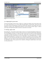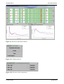
1
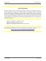
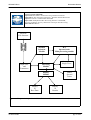
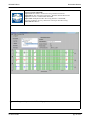
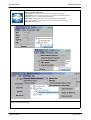
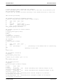
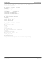
Site Effects Assessment Using Ambient
Excitations
SESAME
European Commission – Research General Directorate
Project No. EVG1-CT-2000-00026 SESAME
WP03 - H/V Technique: Data Processing
Report on the
Multiplatform H/V Processing Software
J-SESAME
WP03 Deliverable D09.03
Department of Earth Science, University of Bergen
Allegt.41, N-5007 Bergen, Norway
Tel: +47-55-583600 Fax: +47-55-5836660 E-mail: [email protected]
June 2003
SESAME WP03
Deliverable D09.03
List of Contents
Summary ........................................................................................................................................................... 2
Chapter 1: Introduction...................................................................................................................................... 3
Chapter 2: The general design of the software .................................................................................................. 3
Chapter 3: Browsing Module ............................................................................................................................ 3
Chapter 4: Window Selection Module .............................................................................................................. 4
Chapter 5: Processing Module........................................................................................................................... 5
Chapter 6: Display Module ............................................................................................................................... 8
Acknowledgements ........................................................................................................................................... 9
FIGURES ........................................................................................................................................................ 10
APPENDIX I ................................................................................................................................................. 18
J-SESAME USER MANUAL (Ver. 1.05) ..................................................................................................... 18
APPENDIX II................................................................................................................................................ 30
SESAME ASCII Format (SAF) ..................................................................................................................... 30
APPENDIX III .............................................................................................................................................. 35
Example input file for the H/V processing ...................................................................................................... 35
List of Contributors (in alphabetical order after the last name)
Kuvvet Atakan
Pierre-Yves Bard
Bladimir Moreno
Pedro Roquette
Alberto Tento
Project coordinator:
Task A Leader:
WP03 Leader:
UiB, Bergen, Norway
LGIT, Grenoble, France
UiB, Bergen, Norway (now at CENAIS,
Santiago de Cuba, Cuba)
ICTE/UL, Lisbon, Portugal
CNR, Milano, Italy
Pierre-Yves Bard, LGIT, Grenoble, France
Kuvvet Atakan. UiB, Bergen, Norway
Kuvvet Atakan, UiB, Bergen, Norway
Contact address:
Kuvvet Atakan
Department of Earth Science, University of Bergen
Allegt.41, N-5007 Beregn, Norway
Tel: +47-55-583600
Fax: +47-55-583660
E-mail: [email protected]
Summary
In the following, we describe a new software solution (J-SESAME) to be used in H/V spectral ratio
technique, which was developed under the framework of the SESAME Project (Site Effects Assessment
Using Ambient Excitations, EC-RGD, Project No. EVG1-CT-2000-00026 SESAME), Task A (H/V
Technique), Work Package 03 (WP03 – H/V Technique: Data Processing). Within the framework of the
SESAME Project one of the work packages is devoted to the development of robust software for data
analysis applying the H/V technique. The main goal of the Work Package 3 (WP03) is to develop a
multiplatform processing software to be used as a standard procedure in processing the microtremor data
using H/V technique. In the J-SESAME, existing algorithms that are used in the H/V data processing are
tested and an optimum solution is applied for the computations. A user-friendly graphical interface is
implemented to allow organizing and browsing the waveform data files easily coupled with several optional
display and output functions. J-SESAME also provides default parameter settings for the different options of
the software, which makes sure that the processing is conducted applying the optimum values.
17-02-04 16:56
pg. 2 of 37
SESAME WP03
Deliverable D09.03
Chapter 1: Introduction
A significant part of damage during strong or moderate ground shaking is associated with local site effects.
Detailed assessment of site effects and the predominant frequencies on which significant amplification
occurs can be obtained using empirical or analytical techniques. Among the empirical techniques, the H/V
spectral ratio of the ambient vibrations (microtremors), has been widely used in microzonation studies due to
its cost-effective nature. Within the framework of the SESAME Project one of the work packages is devoted
to the development of robust software for data analysis applying the H/V technique. The main goal of the
Work Package 3 (WP03), is to develop a multiplatform processing software (J-SESAME) to be used as a
standard procedure in processing the microtremor data using H/V technique. All existing software that was
previously used in processing the microtremor data using the H/V technique are tested and an optimum
solution for the analysis is deduced. The J-SESAME software is developed using the Java Programming
Language, for multiplatform operation capacity. In addition the J-SESAME is designed using a modular
concept for the different parts, allowing flexibility for further developments. The user is guided through the
browsing module (i.e. graphical user interface, GUI) of the software and the window selection and the
processing modules provide the input data selection and computation of the H/V spectral ratios. The display
module is then responsible for producing visualization of the processed data in an easy and flexible way.
This modular development also allows utilizing the best possible solution for the programming language to
be used. In the case of the window selection and processing modules, the software codes are in Fortran,
whereas the browsing and the display modules are developed using the Java Programming language.
In the following, the general design of the software, its functionalities, and the different modules are
explained in detail. A short user manual is also prepared and is included as a separate document in the
appendix (see Appendix I).
Chapter 2: The general design of the software
The general design of the J-SESAME is based on a modular architecture as shown in Figure 1. There are
basically four main modules: the browsing module, window selection module, processing module and the
display module. The main functionalities are integrated through a graphical user interface, which is part of
the browsing module. The display module is also tightly connected to the browsing module, as there is close
interaction between the two modules due to the integrated code development in Java. The window selection
and H/V processing modules act independently and are called from the browsing module to perform specific
computations based on user defined optional parameters. The flowchart of the main processing in the JSESAME software is shown in Figure 2. The location of the software codes and the different parameter files,
as well as the output is organized set by the user through the general configuration parameter settings, which
is included under the “config” pull-down menu. The parameter default values for different options of the
software are also organized under the same menu with relevant titles. The user is expected to check the
default values, which are shown and (if not satisfied) the user is then requested to change them with the
desired values. Once the appropriate parameter values are chosen, they will be applied for the remaining
computations.
In the present version two waveform file formats are supported: GSE and SAF (see Appendix II: SESAME
ASCII Format). In the following chapters, each the four main modules are explained in detail.
Chapter 3: Browsing Module
Browsing module is entirely developed in Java, which is based on a graphical user interface that
communicates with the window-selection and processing modules. The processed data is then visualized
through the display module for manual inspection and different output options are provided (Figure 3). The
main philosophy of the browsing module is to organize the data in individual projects. For each project, the
corresponding waveform files are kept in a directory structure and is accessed through the configuration
17-02-04 16:56
pg. 3 of 37
SESAME WP03
Deliverable D09.03
parameters, which keeps the filenames associated with this project with full path description on the
computer. In addition, the processing parameters that are used in each project are kept in the same project
file under the configuration options.
After defining a new project, the user creates different sites under which the corresponding data collected for
each site are archived in the configuration as a tree-structure (i.e. each project contains several sites and each
site contains several data files). This process allows the user to organize the data into individual sites easily
by dragging on the directory structure or by inserting several files into each site using the mark and copy
options (Figure 4). The default parameters for processing can then be displayed through the pull-down menu
under the configuration (and if desired can be changed) and the entire project can be saved as a “project file”.
A saved project can be uploaded (with the same configuration and parameter settings) for later usage.
Once the data are organized under the project structure, the user then has the possibility to plot the waveform
files (three components on the screen) for manual inspection. After the visual inspection, based on user
defined (or default) parameters, user can select the time-windows either automatically or manually using the
window selection module. The selected windows are then processed by the H/V processing module either as
a single file or as a series of files usually corresponding to the same site. The H/V spectral ratios and the
averages as well as other display options are then plotted using the display module.
In case there is difficulty in selection windows automatically due to transients or other problems in the data
(such as spikes), there are filter options, where the user can apply either low-pass, high-pass or band-pass
filter. The filtered traces are then displayed to the user for window selection. In this process, a comparison is
also made between the windows selected both on the filtered and on the unfiltered trace. The common
windows are then used for further processing. Naturally, only the original unfiltered traces are used for the
H/V ratios. This filtering option allows the user to work also with difficult data sets.
The display module conducts the different plotting options, however, this process is not transparent to the
user. The only thing the user has to do is to click on the output display button when the processing is
completed (for the details of the display options see the following chapters). The different outputs are
displayed through a series of windows.
Chapter 4: Window Selection Module
Besides the manual selection directly from the screen, which is often the most reliable, but also the most time
consuming, an automatic window selection module has been introduced in view of processing large amounts
of data. The objective is to keep the most stationery parts of noise, and to avoid the transients often
associated with specific sources (walks, close trafic). This objective is exactly the opposite of the usual goal
of seismologists who want to detect signals, and have developed specific "trigger" algorithm to track the
unusual transients. As a consequence, we have used here an "antitrigger" algorithm, which is exactly the
opposite: it detects transients but it tries to avoid them.
The procedure to detect transients is very classically based on a comparison between the short term average
"STA", i.e., the average level of signal amplitude over a short period of time, denoted "tsta" in the (typically
around 0.5 to 2.0 s), and the long term average "LTA", i.e., the average level of signal amplitude over a
much longer period of time, denoted "tlta" (typically several tens of seconds). When the ratio sta/lta exceeds
an a priori determined threshold (typical values are between 3 and 5), then an "event" is detected.
In our case, we want to select windows without any energetic transients: it means that we want the ratio
sta/lta to remain below a small threshold value smax (typically around 1.5 – 2) over a long enough duration.
Simultaneously, we also want to avoid noise windows with anomalously low amplitudes: we therefore also
introduce a minimum threshold smin, which should not be reached throughout the selected noise window.
There are also two other criteria that may be optionally used for the window selection:
• one may wish to avoid signal saturation – as saturation does affect the Fourier spectrum. As gain
and maximum signal amplitudes are not mandatory in the SAF and GSE formats, the program
looks for the maximum amplitude over the whole noise recording, and automatically excludes
17-02-04 16:56
pg. 4 of 37
SESAME WP03
•
Deliverable D09.03
windows during which the peak amplitude exceeds 99.5 % of this maximum amplitude. By
default, this option is turned on.
in some cases, there might exist long transients (for instance related to heavy traffic, trains,
machines, …) during which the sta/lta will actually remain within the set limits, but that may be
not representative of real seismic noise. Another option has therefore introduced to avoid "noisy
windows", during which the lta value exceeds 80% of the peak lta value over the whole
recording. By default, this option is turned off.
The program automatically looks for time windows satisfying the above criteria; when one window is
selected, the program looks for the next time window, and allows two subsequent windows to overlap by a
specified amount "roverlap" (default value is 20%).
It has been written as an independent Fortran subroutine, for which:
• The input parameters are the selection parameters (tsta = sta window length; tlta = lta window
length; [smin, smax] = lower and upper allowed bounds for the sta/lta ratio; tlong = noise window
length over which the sta/lta should remain within the bounds; yes/no (1/0) parameters for turning on
or off the saturation and "noisy window" options; overlapping percentage allowed for two
subsequent windows)
• The output parameters are a file with the noise file name, the begin and end times of each selected
window, the recording status of each component : the main processing module then reads this file,
and performs the H/V computation over each selected window.
Chapter 5: Processing Module
Main processing module is developed in FORTRAN90. It conducts H/V spectral ratio computations and the
other associated processing such as DC-offset removal, filtering, smoothing, merging of horizontal
components, etc., on the selected windows for individual files or alternatively on several files as a batch
process. The instrument response is assumed to be removed by the user (in the case of identical components
H/V ratios should not be affected by the instrument response). Main functionalities of the processing module
are described below:
•
•
•
•
•
•
•
FFT (including tapering)
Instrument response removal (not implemented)
Smoothing with the following options
o Konno & Ohmachi
o Moving average
o Linear
o Triangle window
Merging two horizontal components with the following options
o No merging
o Arithmetic mean
o Geometric mean
o Quadratic mean
o Complex merging
H/V Spectral ratio
Average of several (H/V) ratios
Error estimates on spectral ratios
The parameter setting for the above options are controlled through an input file. For the details see the
Appendix III. In the following a summary of the options for the H/V processing is given.
17-02-04 16:56
pg. 5 of 37
SESAME WP03
Deliverable D09.03
1) frequency spacing for output of H/V:
The idea of this option is to specify a smaller sampling in the frequency domain, than the one determined
from the Fourier transform, as much of the information becomes redundant after the smoothing. Other
reasons are a better representation on a log scale or better comparison with other results, which were
differently sampled.
syntax:
freq_spacing=<type>:<arg1>:<arg2>[:<arg3>]
type
fft
fft_red
linear
log
arg1
f_min
f_min
f_min
arg2
f_max
f_max
f_max
arg3
# points
# points
example:
freq_spacing=log:1:10:4
The H/V ratio will then be output for the frequencies 1 2.15 4.64 and 10.
The values of f_min and f_max are positive real numbers, values given in Hertz, f_min has to be smaller than
f_max. the number of points (# points) has to be a positive integer.
2) offset removal
Currently we only foresee the option for offset removal or no offset removal. Maybe later on we can add a
high-pass filtering
Syntax:
offset_rem=<type>[:<arg>]
type:
r_mean
high-pass: frequency
example:
offset_rem=r_mean
The offset is removed
The value of frequency for the high-pass filter is a positive real number, the value should be given in Hertz.
3) tapering window for Fourier Transform
syntax:
taper=<type>:[<arg1>]
type
arg1
arg2
boxcar cos
percentage -
arg3
-
percentage of the window that is affected by the
tapering on both ends
example:
taper=cos:10
The percentage is a positive real number, ranging between 0 (larger than 0) and 50.
4) instrument response correction
17-02-04 16:56
pg. 6 of 37
SESAME WP03
Deliverable D09.03
Currently the instrument response correction will operate on the single time window, therefore it will be
applied in the Fourier domain by multiplication.
syntax:
instrument_resp=<arg>
where arg is either 'yes' or 'no'
example:
instrument_resp = yes
5) smoothing of spectra
syntax:
smooth=<type>:[<arg1>[:<arg2>]]
type
arg1
arg2
none
linear bandwidth box linear smoothing with constant weight in the interval [f-bw/2 f+bw/2]
linear bandwidth tri linear smoothing with triangular weight in the interval [f-bw/2 f+bw/2]
log
percentage box smoothing with constant weight in an interval [f*(1-p/100) f*(1+p/100)]
log
percentage tri smoothing with triangular weight in an interval [f*(1-p/100) f*(1+p/100)]
konno-ohmachi b-value - b-value for the smoothing window as defined in the Konno-Ohmachi article
example:
smooth=log:10:tri
Each spectrum is smoothed on a logarithmic scale with bandwith 10 percent and triangular weighting
The value of the bandwidth is a positive real number in Hertz. The percentage is a positive real, with units
‘%’, common values would be eg. 5 or 10. The Konno-Ohmachi b-value is defined in Konno and Ohmachi
(1998), BSSA Vol 88, pp228-241, and it has positive values, eg. 10, 20 or 30.
6) merging of horizontal components
syntax:
merge_type=<type>
type
arithmetic
geometric
quadratic
(H_ew+H_ns)/2
sqrt(H_ew*H_ns)
sqrt(H_ew^2+H_ns^2)
7) output of H/V for the single components
syntax:
single_component=<arg>
arg: 'yes' or 'no'
If yes is selected, the output file will contain the columns
frequency, average H/V, error, average H_ns/V, error, average H_ew/V, error
If no is selected, the output file will contain only the columns
frequency, average H/V, error
8) type of averaging the multiple windows
syntax:
average_type=<type>
17-02-04 16:56
pg. 7 of 37
SESAME WP03
Deliverable D09.03
type:
linear
log
9) output of single window information
syntax:
single_win_out=<arg>
arg is either 'yes' or 'no'
In case of 'yes', for each time window a separate output file is created. The name of the file is the base output
file name extended by '_win_###', ### indicating the number of the time window in the sequence of file#2.
Each file contains the columns
frequency, spectrum vertical, spectrum NS, spectrum EW, merged H/V, H/V ns, H/V ew
Chapter 6: Display Module
The ‘Display Module’ was developed using the Java programming language. During the preparations
interactions were made with groups working on the main processing module to coordinate the data input and
output. In the following, the main functionalities of the display options are given.
•
•
•
•
•
•
•
•
In general zooming is possible on all plots by left mouse button click and drag. Clicking once on
the plot with left mouse button returns back to original trace.
Right hand button of the mouse is used for highlighting a selected window. Clicking once again
will give the option of deleting the window (available only in the browsing module).
In the output window the title used is the name of the output file (Figure 5).
In the output window all processing parameters present in the parameter file are shown (Figure 5).
A legend that shows the meaning of each of the curves (Figures 5-7).
It is possible to change the settings of each chart by clicking on the small box on the upper right
corner. The settings include:
o The colours
o The line patterns and thickness
o Showing (or not) the chart gridlines
o Showing (or not) box axis
o The font properties of the various fonts
o Which curves to show
o Saving format options
The windows are resizable.
User option to change between logarithmic and linear scales. The user is also able to change the
limits in the scale.
17-02-04 16:56
pg. 8 of 37
SESAME WP03
Deliverable D09.03
Acknowledgements
This project (Project No. EVG1-CT-2000-00026 SESAME) is supported by the European Commission –
Research General Directorate. Apart from the authors of this report, a number of individuals have provided
valuable contributions at different stages of the development. We thank Paula Teves-Costa (ICTE/UL,
Lisbon), Jean-Luc Chatelain and Bertrand Guillier (RD, LGIT, Grenoble), and Jens Havskov (UiB, Bergen)
for constructive suggestions, to Fabrizio Cara (INGV, Rome), Anne-Marie Duval (CETE, Nice) for testing
the earlier version and suggesting the default parameter values. We also thank Fortunat Kind (ETH, Zurich)
who has contributed to the development of the processing module during the initial stages. Finally, we thank
all the SESAME project participants from the different participating institutions, who have contributed to JSESAME in different ways.
Appendix I: J-SESAME User Manual (Ver.1.05)
Appendix II: SESAME ASCII Format (SAF)
Appendix III: Example input parameter file for H/V processing
This deliverable (including the report, figures and appendices) is available on a CD, which can also be
downloaded from the anonymous ftp site of the University of Bergen at the following address:
ftp://ftp.ifjf.uib.no/pub/sesame/REPORT/WP03/DELIVERABLE/
17-02-04 16:56
pg. 9 of 37
SESAME WP03
Deliverable D09.03
FIGURES
17-02-04 16:56
pg. 10 of 37
SESAME WP03
Deliverable D09.03
Project Acronym: SESAME
Project Title: Site Effects Assessment Using Ambient Excitations
Supported by: The European Commission – Research General Directorate
Project No: EVG1-CT-2000-00026 SESAME
Report Title: Multiplatform H/V Processing Software: J-SESAME,
University of Bergen, Norway. WP03 H/V Technique: Data Processing.
Deliverable No: D09.03
Projects:
File-structure
Window
Selection
Module
H/V
Spectral ratio
Main processing module
Interactive
Single Trace
Browsing
Module
Input Files
and
Parameters
Display
Module
Display
of
Raw Data
Batch
Several
Traces
Display
of
Results
Figure 1 : The general design of the J-SESAME Software. The four main modules are shown in bold.
17-02-04 16:56
pg. 11 of 37
SESAME WP03
Deliverable D09.03
Project Acronym: SESAME
Project Title: Site Effects Assessment Using Ambient Excitations
Supported by: The European Commission – Research General Directorate
Project No: EVG1-CT-2000-00026 SESAME
Report Title: Multiplatform H/V Processing Software: J-SESAME,
University of Bergen, Norway. WP03 H/V Technique: Data Processing.
Deliverable No: D09.03
Browsing Module
Local
Storage
Filelist.inp
Winparameter.inp
Project_files
in a directory structure
including the
configuration
parameters (i.e.
File_names and path
of input waveforms;
File_names for output
Filter
YES
Filtertemp
sesame.txt
NO
Filter the trace
“Filename_out”_
SAF_fi
Window
Selection Module
Winselection.out
HVprocess.inp
H/V Processing
Module
Numerical
output files
Display
Module
Graphical
output files
Figure 2 : Flowchart of the main processing in the J-SESAME software.
17-02-04 16:56
pg. 12 of 37
SESAME WP03
Deliverable D09.03
Project Acronym: SESAME
Project Title: Site Effects Assessment Using Ambient Excitations
Supported by: The European Commission – Research General Directorate
Project No: EVG1-CT-2000-00026 SESAME
Report Title: Multiplatform H/V Processing Software: J-SESAME,
University of Bergen, Norway. WP03 H/V Technique: Data Processing.
Deliverable No: D09.03
Figure 3: The general layout of the J-SESAME graphical user interface.
17-02-04 16:56
pg. 13 of 37
SESAME WP03
Deliverable D09.03
Project Acronym: SESAME
Project Title: Site Effects Assessment Using Ambient Excitations
Supported by: The European Commission – Research General Directorate
Project No: EVG1-CT-2000-00026 SESAME
Report Title: Multiplatform H/V Processing Software: J-SESAME,
University of Bergen, Norway. WP03 H/V Technique: Data Processing.
Deliverable No: D09.03
Figure 4 : The different pull-down menu’s of the J-SESAME for project description, parameter
configuration and processing.
17-02-04 16:56
pg. 14 of 37
SESAME WP03
Deliverable D09.03
Project Acronym: SESAME
Project Title: Site Effects Assessment Using Ambient Excitations
Supported by: The European Commission – Research General Directorate
Project No: EVG1-CT-2000-00026 SESAME
Report Title: Multiplatform H/V Processing Software: J-SESAME,
University of Bergen, Norway. WP03 H/V Technique: Data Processing.
Deliverable No: D09.03
Figure 5 : The display options of the J-SESAME. Average H/V spectral ratio for the merged horizontal
component with standard deviation are shown in diferent colors.
17-02-04 16:56
pg. 15 of 37
SESAME WP03
Deliverable D09.03
Project Acronym: SESAME
Project Title: Site Effects Assessment Using Ambient Excitations
Supported by: The European Commission – Research General Directorate
Project No: EVG1-CT-2000-00026 SESAME
Report Title: Multiplatform H/V Processing Software: J-SESAME,
University of Bergen, Norway. WP03 H/V Technique: Data Processing.
Deliverable No: D09.03
Figure 6 : Plotting options of the J-SESAME. Average of the individual H/V spectral ratios for the N-S
and the E-W components (standard deviation is shown in different colors).
17-02-04 16:56
pg. 16 of 37
SESAME WP03
Deliverable D09.03
Project Acronym: SESAME
Project Title: Site Effects Assessment Using Ambient Excitations
Supported by: The European Commission – Research General Directorate
Project No: EVG1-CT-2000-00026 SESAME
Report Title: Multiplatform H/V Processing Software: J-SESAME,
University of Bergen, Norway. WP03 H/V Technique: Data Processing.
Deliverable No: D09.03
Figure 7 : The ploting options of the J-SESAME. The indicidual H/V spectral ratios (of the merged and
the two horizontal components) for a selected time window (in red) is shown on the lower left diagram.
The diagram on the lower right shows the spectra for the three components.
17-02-04 16:56
pg. 17 of 37
SESAME WP03
Deliverable D09.03
APPENDIX I
J-SESAME USER MANUAL (Ver. 1.05)
17-02-04 16:56
pg. 18 of 37
SESAME WP03
Deliverable D09.03
JSESAME
USER MANUAL
Version 1.05
June 2003
Table of contents
1. Introduction
2. Requirements
3. Installation
4. Getting Started
5. Using JSEISAN
5.1.Configuration of the program
5.2.Creating a new project
5.3.Plotting data files
5.4.Selecting windows
5.4.Plotting filtered traces
5.5.Computing H/V spectral ratio
5.6. Showing output results
5.7. Setting graph properties and creating images of the output results
1. Introduction
JSESAME is a JAVA application for providing a user-friendly graphical interface for H/V spectral
ratio technique used in local site effect studies. The program uses the functions of automatic
window selection and H/V spectral ratio by executing external commands. The automatic window
selection and H/V process are standalone application developed in Fortran. JSESAME is mainly a
tool for organizing the input data, execute window selection and processing, and display the
processing results. The software operates in both Unix and Windows environments.
2. Requirements
The following tool has to be installed in the Operating System:
9 Java Runtime Environment (JRE). You can download the files relevant for your operating
system from the following web site: http://www.sun.com
3. Installation
Two ZIP files are provided for Unix and Windows environments. The ZIP include three directories
with the following files (Windows environment):
In Hvprocess directory
17-02-04 16:56
pg. 19 of 37
SESAME WP03
Deliverable D09.03
hvproc0_1.exe : main processing module for H/V ratio
hvsource.zip : source files
In WindowSelection directory
Winselection.exe : automatic window selection
winsource.zip: source files
In Jsesame directory
jsesame.jar : java classes and source code
jsesame.bat : script for executing the Java application “Jsesame”
jsesame.pdf : user manual
images : directory with tools-bar images
4. Getting started
Once the ZIP file is uncompressed, user must open a Unix or DOS console, go to Jsesame directory
and start the program from the prompt line as:
jsesame
Figure 1. Main window
5. Using JSESAME
The user interaction with JSESAME (Figure 1) can be classified as: (1) Organizing the information,
(2) processing the information and (3) displaying the results. The interface has a main window
17-02-04 16:56
pg. 20 of 37
SESAME WP03
Deliverable D09.03
where the user can create a new project or loaded an existing project, plot the traces on the screen,
perform automatic or manual window selection, apply the H/V spectral ratio computations and see
all the results in a user-friendly interface. Only two waveforms data format are accepted: GSE and
SAF (SESAME ASCII Format). The extension of the data files is required to be one of these words
(GSE or SAF).
5.1. Configuring the program
JSESAME has several configuration variables to be set up by the user. In order to configure the
variables, you have to click the item menu <Config> (Figure 2). The configuration parameters are
shown in five dialog boxes. The first one is for configuring the automatic window selection (Figure
3), the second for the manual window selection, the third for the H/V processing module (Figure 4),
the fourth for the filters parameters (Figure 5) and the last one for general configuration parameters
(Figure 6). Note it is very important set the correct path for the window selection and processing
module programs since they are external command call by JSESAME.
Figure 2. Configuration menu
5.2. Creating a new project
The structure of the project has a tree shape (Figure 1) where the data files are grouped by sites
when several noise measurements are performed for a single location. Data files grouped in the
“Unassigned_file” node are treated independently. That is the user has only one data file for each
site. Each node in the tree has several parameters shown on the right side of the tree. The “Site
name” and the “Output File name” parameters can be modified by the user. The changes are applied
after pressing the RETURN key. Data file nodes can be dragged and dropped through the tree
structure. For inserting new data files or sites and removing nodes from the project, users can press
the corresponding button shown on the left site of the tree (Figure 1). The tree structure allow for
multi-selection of nodes, which means that batch processing can be performed for several sites or
individual data files. The project can be saved by using the item menu <project> (Figure 7) or by
using the tools bar shown below the menu (Figure 1).
17-02-04 16:56
pg. 21 of 37
SESAME WP03
Deliverable D09.03
Figure 3. Automatic window selection parameters
Figure 4. Processing module parameters for H/V spectral ratio
5.3. Plotting data files
The highlighted or selected data-file can be plotted by pressing the button <Plot traces>. All the
selected windows will be shown (Figure 8). Zooming can be done by clicking the left button of the
mouse, then drag the mouse and release the button at the end of the selected time of the window.
Clicking the left mouse button on anywhere on the plot will take you back to the original trace
before zooming.
17-02-04 16:56
pg. 22 of 37
SESAME WP03
Deliverable D09.03
Figure 5. Filter options
Figure 6. General parameters
5.4. Selecting windows
Windows can be selected automatically or manually. The manual window selection can be done if
the check-box labeled as “Manual window selection” (Figure 8) is active. The window is selected
using the same procedure as zooming action. Individual windows can be removed by clicking the
right button of the mouse twice: one click for selecting the window and another click for the
deleting action. Automatic window selection can be performed in four different ways (Figure 9).
The first one is applied to the original traces. The second is applied to the filtered trace with the
filter selected in the <Config> option. The third is the common windows between the original and
the filtered traces. The last option keeps the same selected windows of the first file for the rest of
17-02-04 16:56
pg. 23 of 37
SESAME WP03
Deliverable D09.03
the selected files. This option makes sense when the user highlights (select) a group of files from
the project.
Figure 7. Project options
Figure 8. Zoomed traces with the selected windows
5.5. Plotting filtered traces
The selected data-files can be filtered with the previous selected filter in the <Config> option
(Figure 5) and then plotted on the screen. This option is available within the <Processing> menu
item (Figure 9). The selected windows for the plotted data-file are also shown. Zooming on the
filtered traces can be performed as explained in section 5.3.
17-02-04 16:56
pg. 24 of 37
SESAME WP03
Deliverable D09.03
Figure 9. Processing options
5.6. Computing H/V spectral ratio
The processing module (option shown in Figure 9) is applied according to the selected nodes in the
tree. If the selected node is a site, then all the selected windows of the data-files collected for this
site will be used for computing the average H/V spectral ratio. Output for each window also can be
obtained by setting up the configuration parameters of the processing module (Figure 4). Batch
processing will be performed when several sites or data-files are selected.
5.6. Showing output results
By pressing the <View Output> button (Figure 8) the user can navigate through three dialog boxes.
The first dialog box (Figure 10) shows the H/V spectral ratio of the merged horizontal components.
The second dialog box (Figure 11) shows the H/V spectral ratio for each one of the NS and EW
components. The third one (Figure 12) shows the spectral ratio of the merged (H), NS and EW
horizontal components and the spectra of Z, NS and EW for each individual window, if “output
single window information” is selected in the configuration parameter of the processing module
(Figure 4). To select an individual window the user has to click the right button of the mouse on it.
Zooming action can be done over the spectrum using the same procedure explained in section 5.3.
The individual values of the spectrum can be shown by clicking the middle button of the mouse
over the spectral curve.
17-02-04 16:56
pg. 25 of 37
SESAME WP03
Deliverable D09.03
Figure 10. Spectral ratio for merged horizontal components
5.7. Setting graph properties and creating images of the output results
For each graph shown in Figure 10,11 and 12 there is a small box in the upper right corner without
any label. By clicking there the properties and scale of the graph can be modified and images of the
graph can be created (Figure 13a). The button <Properties and series> pop up a dialog box (Figure
13b) where line type, width and colour (Figure 13c) can be changed for each spectral curve. The
button <Scales> pop up a dialog box (Figure 13d) where the minimum, maximum and scale for
each one of the vertical and horizontal axes can be modified. The button <Save> allows to create an
image of the graph.
17-02-04 16:56
pg. 26 of 37
SESAME WP03
Deliverable D09.03
Figure 11. Spectral ratio for each NS and EW horizontal component
17-02-04 16:56
pg. 27 of 37
SESAME WP03
Deliverable D09.03
Figure 12. Result for individual windows
Figure 13a. Graph properties
Figure 13b. Selection of the components
17-02-04 16:56
pg. 28 of 37
SESAME WP03
Deliverable D09.03
Figure 13c. Properties of the Spectral curve
Figure 13d. Scale properties for the spectral curve
17-02-04 16:56
pg. 29 of 37
SESAME WP03
Deliverable D09.03
APPENDIX II
SESAME ASCII Format (SAF)
17-02-04 16:56
pg. 30 of 37
SESAME WP03
Deliverable D09.03
Format of the input waveform file: SESAME ASCII Format (SAF)
The SESAME ASCII Format (SAF) file is organized in 3-columns (corresponding to 3-channels)
and the parameters that must be included in the header are:
-Station/Site code
-Start date and time
-Sampling frequency
-Number of samples (data points)
-Component-1 definition (i.e. to indicate which column refers to which channel)
-Component-2 definition
-Component-3 definition
-Unit of the data points
Key words and other details would have to be handled by the developers.
Therefore the structure of such SESAME data file should be:
- First line: "SESAME ASCII data format (saf) v. 1 "
- Header information
- Empty lines are allowed
- Comments can be added provided that the first character in the row is "#"
- Keywords are not case sensitive
- Separator between keywords and their values is "="
- The order of the keywords is irrelevant
- Blanks can be added everywhere
- Data begin after this separator line: "####--------------------"
- Data are written in three columns free format
- Column 1 must correspond to the Vertical channel, columns 2 and 3 to the horizontal ones
Mandatory keywords are :
- STA_CODE : station/site code (In the GSE2.0 format this parameter is at most 5 characters long)
- START_TIME : start date and time - year month day hour minute second (e.g. 1999 4 23 0 3
44.78 )
- SAMP_FREQ : sampling frequency in Hertz
- NDAT : number of samples
- CH0_ID : component 1 definition - It should be the vertical channel. It is a label. (In the GSE2.0
format this parameter is 3 characters long)
- CH1_ID : component 2 definition - horizontal
- CH2_ID : component 3 definition - horizontal
- UNITS : label (e.g. m/s)
Supposing that the horizontal components are at 90 degrees between each other, we still need to add
an OPTIONAL parameter, which deals with sensor orientation.
- NORTH_ROT : is the orientation of the first horizontal component (channel 1 - column 2) from
North clockwise (degrees)
17-02-04 16:56
pg. 31 of 37
SESAME WP03
Deliverable D09.03
The following keywords/codes are available from the header:
• reference code of the sensor response (instrument response file)
• sampling_rate in Hertz (eg. 125Hz)
• date and time: start time of the trace as accurate as possible
• accuracy of timing
• sensor type (accelerometer/seismometer)
• instrument-ID digitizer (serial number)
• instrument-ID sensor (serial number)
• acquisition system
• conversion factor: counts -> Volt (V/count)
• transduction: Volt -> physical meaning (V/m/s)
• units of data in file (counts, or whatever, just identifying it)
• number of data points
• comment line defining Vertical, NS, EW
• saturation of digitizer
• site code of exactly six characters (eg. BSL_12)
• Station coordinates on separate lines, X,Y,Z
• project name
• arbitrary number of comment lines
• separator line before the data
• earthquake information as defined as for the Pitsa format
In general the processing should be possible without most of the above information. But the
following are strictly required:
• sampling_rate in Hertz (eg. 125Hz)
• number of data points
• channel information is needed, but it is fixed in the format
Although the instrument response information is not mandatory, the following two options may be
of interest for the processing:
• reference code of the sensor response (instrument response file)
• saturation of digitiser in units of data
The remaining options are recommended.
Filenames of SESAME ASCII
1) free file name, extension of the name will be .saf, such that the format can be identified from
the extension
2) The
suggested
filename
contains
site
code,
date
and
time:
NNNNNN_yyyyMMdd_hhmm.saf
17-02-04 16:56
pg. 32 of 37
SESAME WP03
Deliverable D09.03
Following is an example of a SAF file:
SESAME ASCII data format (saf) v. 1
(this line must not be modified)
# The SESAME ASCII Format can contain an arbitrary number of comment
# lines starting with '#' in the header. Parameters are specified on
# lines starting without # character, followed by a keyword separated
# with a '=' sign from the value of the key. The keyword name can be in
# lower
# or upper case letters, no distinction is made in the interpretation.
# No empty lines are allowed in the header.
# The first line indicates the name of the file format,
# for automatic format identification tools.
#
# Two compulsory parameters have to be specified
# the sampling rate and the number of points.
#
# All other parameters are optional, but the response and saturation
# information
# is highly recomended.
#
# Data begin after this line : "####--------------------------------"
# Data are organized in colums in this order : Vertical, Horizontal_1,
# Horizontal_2
# Horizontal_1 generally is N-S, for different orientation parameter
# NORTH_ROT can
# be set.
# Data can be real or integer
#
#
# sampling frequency in Hertz
SAMP_FREQ = 125
# number of samples (integer)
NDAT = 1200
# date and time of the first sample, read as 5 integers, one real
START_TIME=2002 4 26 17 03 12.1233324
# accuracy of the timing, in seconds
#very large values indicate manual time setting
# GPS ~0.001, DCF ~0.01
TIME_ACCURRACY= 0.001
# Sensor type (accelerometer, seismometer)
SENSOR_TYPE = accelerometer
# Sensor serial number (character string)
SENSOR_ID = Q332
# Sensor name (character string)
SENSOR_NAME = Lennartz 5s
# Response file code (name of the file in the response directory)
RESPFILE = mark1s_098
# Acquisition system (character string)
ACQ_SYSTEM = MARS88
# Digitizer serial number (interpreted as character string)
DIGITIZER_ID = 345
# saturation value of the digitizer in UNITS
SATURATION = 23056
# conversion factor ( V/count)
CONV_FACTOR = 1234.5
# transduction factor (Volts/m/s or Volts/m/s^2)
TRANS_FACTOR = 12345.6
# Eigen frequency of the sensor
SENS_EIGFREQ = 1
# Damping factor of the sensor
SENS_DAMPING = 0.7
# Code for the site (exactly 6 characters)
17-02-04 16:56
pg. 33 of 37
SESAME WP03
Deliverable D09.03
STA_CODE= NCE_12
# Station coordinate type, 0= lat/lon, 1= km of local coordinate,
# elevation is always in km
STA_COORD_TYPE = 0
# coordinates are one real number: 45 30' -> 45.5
STA_X = 45.73
STA_Y = 7.009
STA_Z = 0.235
# project name
PROJECT_NAME = example data format project
#
# Earthquake data can be specified with the Pitsa keywords:
#
# Event coordinate type, as station coordinate type
EVT_COORD_TYPE = 0
# Event location
EVT_X = 34.5432
EVT_Y = 5.876
EVT_Z = 0.786
# Event time (origin time)
EVT_TIME = 1989 3 23 17 4 12.345
# Event comment
EVT_COMMENT = Lisbon quake
# Station comment
STA_COMMENT = bedrock
# event azimuth (from north clockwise)
EVT_AZ = 270
# event backazimuth (from north clockwise)
EVT_BACK_AZ = 23.345
# event hypocentral distance (km)
EVT_HYPO_DIST = 30
# event epicentral distance (km)
EVT_EPI_DIST = 3000
# Event magnitude definitions:
EVT_MAG = 7.3
# magnitude definitions with specific magnitudes
# possible keys: EVT_LOCAL_MAG, EVT_BODY_MAG, EVT_SURFACE_WAVE_MAG,
#
EVT_DURATION_MAG, EVT_MOMENT_MAG
# Orientation of Horizontal_1 component from North clockwise (degrees)
NORTH_ROT
# units of the values below in the data (label)
UNITS = m/s
#
# Vert, NS, EW
####------------------------------------------------------13
214
898
13
214
898
13
214
898
13
214
898
13
214
898
13
214
898
13
214
898
13
214
898
13
214
898
13
214
898
13
214
898
13
214
898
13
214
898
13
214
898
13
214
898
13
214
898
13
214
898
13
214
898
13
214
898
17-02-04 16:56
pg. 34 of 37
SESAME WP03
Deliverable D09.03
APPENDIX III
Example input file for the H/V processing
17-02-04 16:56
pg. 35 of 37
SESAME WP03
Deliverable D09.03
# example parameter file
# lines starting with # character are comments
# the following part of this file refers only to what will be processed by the
min processing routine,
# there will be further sections relating to the window selection or what ever.
### section processing
## possible options for frequency spacing
# syntax: freq_spacing:<type>:<arg1>:<arg2>[:<arg3>]
#
#
type arg1 arg2 arg3
#
fft
#
fft_red
f_min f_max #
linear
f_min f_max # points
#
log
f_min f_max # points
freq_spacing:log:0.1:25:800
## possible options for offset removal
# syntax
# offset_rem:<type>[:<arg>]
# type:
# no
# r_mean
# high-pass: frequency
offset_rem:high-pass:0.02
## tapering
# syntax:
# taper:<type>:[<arg1>]
#
#
type arg1 arg2 arg3
#
boxcar
#
cos
percentage the
#
#
taper:cos:5
-
percentage of the window that is affected by
tapering on both ends
## instrument correction
# syntax:
# instrument_resp:<arg>
#
# where arg is either 'yes' or 'no'
#
instrument_resp:yes
## smoothing section
# syntax:
# smooth:<type>:[<arg1>[:<arg2>]]
#
# type
arg1 arg2
# none
# linear
bandwidth
box
linear smoothing with constant weight in the
interval [f-bw/2 f+bw/2]
# linear
bandwidth
tri
linear smoothing with triangular weight in the
interval [f-bw/2 f+bw/2]
# log percentage box
smoothing with constant weight in an interval
[f/(1+p/100) f*(1+p/100)]
# log percentage tri
smoothing with triangular weight in an interval
[f/(1+p/100) f*(1+p/100)]
17-02-04 16:56
pg. 36 of 37
SESAME WP03
# konno-ohmachi bandwidth
#
smooth:konno-ohmachi:20
Deliverable D09.03
- bandwith for the smoothing window
## merging of horizontal components
# syntax:
# merge_type:<type>
#
# type
# arithmetic
(H_ew+H_ns)/2
# geometric sqrt(H_ew*H_ns)
# quadratic sqrt(H_ew^2+H_ns^2)
#
merge_type: geometric
## output of single components
# syntax:
# single_component:<arg>
#
# arg: 'yes' or 'no'
single_component:no
## average of horizontal components
# syntax:
# average_type:<type>
#
# type
# linear
# log
average_type:log
## output of single window information]
# syntax:
# single_win_out:<arg>
#
# arg is either 'yes' or 'no'
single_win_out:no
### end processing
# maybe some further options not related to the processing
17-02-04 16:56
pg. 37 of 37