1
Additional technical information for
CanSat competition 2014
Information for users of the European CanSat kit
prototype 2013
Reference:
CSUK-T01
Version:
2.0
Date:
Valid from:
25/09/2013
25/09/2013
Issued By:
Reviewed By:
Hein Olthof
Eric Smit
Additional technical information for CanSat competition 2014
Reference: CSUK-T01
Version: 2.0
Page 2/53
Change record
Version
Date
Chapter
Remarks
1.0
17 January 2013
all
Creation
2.0
25 September 2013
all
General review
© T-Minus Engineering. This document is composed for STEM center York for the aid of the European
CanSat competition 2014.
Additional technical information for CanSat competition 2014
Reference: CSUK-T01
Version: 2.0
Page 3/53
Table of contents
Introduction ......................................................................................................................................................................................5
Defining missions ...........................................................................................................................................................................6
Budget constraints..........................................................................................................................................................................7
Presentation and reports. .............................................................................................................................................................8
Presentation.................................................................................................................................................................................8
Reports ..........................................................................................................................................................................................8
Introduction to measurement tools ..........................................................................................................................................9
Length ............................................................................................................................................................................................9
Ruler ................................................................................................................................................ 9
Caliper ........................................................................................................................................... 10
Angles ......................................................................................................................................................................................... 11
Protractor ...................................................................................................................................... 11
T-square ........................................................................................................................................ 12
Mass ............................................................................................................................................................................................. 13
Scale .............................................................................................................................................. 13
Electronics: voltage, current, resistance.......................................................................................................................... 14
Multimeter .................................................................................................................................... 15
Example of CanSat setup with the European CanSat kit ............................................................................................... 16
Parachute design and construction ....................................................................................................................................... 18
The physics behind the drag parachute .......................................................................................................................... 19
Shapes of drag parachute .................................................................................................................................................... 21
Lifting parachute ..................................................................................................................................................................... 23
Testing your parachute ......................................................................................................................................................... 24
Introduction to electrical circuits ........................................................................................................................................... 25
Reading of a circuit ................................................................................................................................................................ 25
Components .............................................................................................................................................................................. 26
Sensors ....................................................................................................................................................................................... 29
Communication........................................................................................................................................................................ 33
Additional technical information for CanSat competition 2014
Reference: CSUK-T01
Version: 2.0
Page 4/53
Batteries and power system ..................................................................................................................................................... 34
Battery types............................................................................................................................................................................. 34
Advantages and disadvantages .......................................................................................................................................... 35
Calculations with a battery.................................................................................................................................................. 35
Battery tips and tricks ........................................................................................................................................................... 36
Introduction to soldering and circuit assembly ................................................................................................................. 38
Soldering.................................................................................................................................................................................... 39
Radio communication................................................................................................................................................................. 42
Introduction to programming .................................................................................................................................................. 45
Data inconsistencies .............................................................................................................................................................. 46
Introduction to data analysis ................................................................................................................................................... 47
From data to measurements: calibration........................................................................................................................ 47
Results presentation .............................................................................................................................................................. 49
Other resources and further information............................................................................................................................. 53
Additional technical information for CanSat competition 2014
Reference: CSUK-T01
Version: 2.0
Page 5/53
Introduction
This document was written as a technical add on for the CanSat kit user manual for the STEM center in
York. Since the STEM center works in 2013/2014 with the European CanSat kit prototype, it lacked some
technical information necessary for completing a CanSat competition.
This document is divided into a project management section, a mechanical section and an electronics
section. The chapters are written for students and teachers in mind and try to teach technical background
as well as hands-on skills vital for completing a successful CanSat project.
Additional technical information for CanSat competition 2014
Reference: CSUK-T01
Version: 2.0
Page 6/53
Defining missions
The definition of a mission is very important, because it will determine the complete CanSat project. A
mission statement is a statement that will give your project focus. It should be clear and concise. When
trying to write a good mission statement, make sure to do a couple of iterations.
Any mission will start with a “why”-question. Why are you interested in A or B? It could well be that what
you want to do is not the best method to do it. What we like to see is a mission and a number of options
to fulfill the mission. The reasons why your design was the best option should be made clear. For the
primary mission, the reason why pressure and temperature are measured is because we can determine the
altitude from that. So the primary mission would be to determine the altitude of the CanSat with the use
of the temperature and pressure sensor. If the last part was not demanded by the organization other
methods of determining the altitude of the CanSat would be good as well. But the team must explain why
they made certain decisions.
An example of a mission statement that is not so strong: ”Our team wants to make video recordings of
the CanSat descent”. This is not a good mission statement, because the “why”-part is missing. An
improvement would be “The CanSat will determine the number of animals in a 4 km^2 area centered on
the launch site”.
In a nutshell, the mission statement is an answer to the question “what does our CanSat team want to
achieve and why?” Now perhaps it is easy to think of all kind of things that one can do with a CanSat but
the “and why?” part of the question is fundamental.
Additional technical information for CanSat competition 2014
Reference: CSUK-T01
Version: 2.0
Page 7/53
Budget constraints
Every project has limited resources. Examples of resources are production capacity, financial, volume and
lots of others. In this chapter the use of a budget to manage the limited resources is discussed. The goal
of a budget is to have an overview of the status of the resources so that the project does not overrun the
requirements and other constraints.
Any budget starts with a topic, the most obvious is financial. Then the requirements determine the
amount that can be used. This can be a constraint, like the cost of the CanSat, but also an estimate of the
resource that needs to be made available. Now, it needs to be shown that the project fulfills the
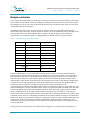
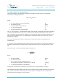
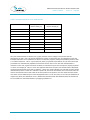
requirements. This is done by means of a budget table, an example of which is given in Table 1.
Table 1: an example of a simplified budget
Expected [In leafs]
Actual [1/1/2001]
School
10
10
Sponsors
5
2
15
12
Electronics
6
9
Travel
6
6
Total
12
15
Result
3
-3
Income
Total
Expenses
From this budget table, it can be seen clearly that the sponsor income is less than expected and the
expenses are more than expected, resulting in a shortage. This is a serious problem. If you would have
such a situation with mass or volume the CanSat would not be allowed to fly. So it is very important to
keep track of all resources. In the project a number of requirements have/will be given. One of these
requirements is with respect to the amount of resources that can be spent on the CanSat. A budget table
is a great tool to be informed about the status of the expenditures and income. Any budget table will
have three parts an estimation, realization and closing. They will be discussed in short.
The first thing is to determine the budget: what resources are available to spend. In the CanSat case, this
can be limited both by what is available from the school or sponsors and what is allowed within the rules.
Then an estimation of the expected expenditures must be made. Start with a group brainstorm about
what is needed and then try to make a good estimation about the cost. Also allow for some margin,
because there will be setbacks. Now you have a great idea with an awesome CanSat but you need to have
it finished in time. Work on a time budget; estimate what you need, estimate the time you can spend and
again some margin, as you might have setbacks. In general it is better to have a modest CanSat done with
a high quality of work compared to a complex CanSat almost ready and with low quality work. Also
important is planning, a team member can have time but he might not be able to work because a sensor
is not yet delivered.
Hint: generally we overestimate our own abilities. With a budget you can recognize this and possibly fix it.
Additional technical information for CanSat competition 2014
Reference: CSUK-T01
Version: 2.0
Page 8/53
Presentation and reports.
In order to communicate in a large project, it is essential to have good presentation skills and a good,
concise and clear reporting style. Both presentations and reporting are needed for your CanSat project. A
small report is needed to relay all project-information to the judges of the CanSat competition.
Furthermore, a small presentation is needed to accompany this report and to give more digestive
information to people who did not read your report.
Presentation
To give a presentation for a lot of people is something that everybody dislikes in the beginning. Some
people really find it scary in the beginning, but it is a skill which everybody can learn very quickly. Try to
practice a couple of times for a full classroom. Don’t learn your presentation “by heart”, because it could
be the case that you are going to talk faster and faster when you do the final version in public. Some
small tips for presenting:
•
•
•
•
Try to be as relaxed and normal as possible. This is not some Shakespeare play, it is a technical
presentation.
Speak slowly, don’t try to rush everything to the end. If you have a watch or a small clock, take it
with you on the stage. You will directly see how much time you have left for your presentation.
You can either slow down or accelerate if the time demands it.
Know your stuff. If you did the research, you will be the person who knows everything there is to
know. For questions about the subject you are the best person to answer it. If you don’t know the
answer then you can always say that it is a good question and you will look for an answer and
contact the person after the presentation.
Have fun. After a while you are not as scared anymore for speaking in public. Try to enjoy it,
people in the audience will notice it and find it much easier to listen to it.
Reports
For writing reports the ESA CanSat project has some nice self-explaining report templates. Try to follow
these templates by filling in the required information. In reporting it is always difficult to give enough
information without overloading people with too much information. Try to put details like electronic
schematics in an appendix. The document itself (without the appendices) should be a readable document
for a technically educated person.
Additional technical information for CanSat competition 2014
Reference: CSUK-T01
Version: 2.0
Page 9/53
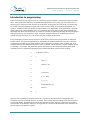
Introduction to measurement tools
During the production of your CanSat, you will very likely need to measure certain quantities: the
diameter of your parachute, the mass of your CanSat, or maybe its battery voltage. To do this, you will
need the proper tools. Most of them, such as the ruler or the scale, you are probably familiar with. Other
tools, such as the caliper, may be new to you. This chapter will describe some of the tools that you will
most likely want to use. Also, the correct usage of them is explained. The chapter is divided into four
sections, in each of which a certain measurable quantity, such as length or mass, is treated.
Length
The first and probably most important quantity that is measured is the size of objects. This can be the
height of a CanSat, or the diameter of a thread for example. The quantity we are measuring in these cases
is length, defined as the distance between two known points. Length can be defined in many units. These
units are roughly defined in two systems: the imperial system and the metric system. The imperial system is
the most common system used in the US and the UK. The metric system is mainly used in Europe. The
units in which a length is most conveniently expressed depends on the actual size that is measured. The
height of the CanSat is probably expressed in millimeters (mm), centimeters (cm) or inches (in), and the
distance from your house to your school is most likely expressed in kilometers (km) or miles (mi). For the
translation between one unit to the other, linear translation rules are defined. These express how many of
one unit add up to another unit. For example, 100 centimeters make one meter, and 1000 meters make
one kilometer. The other way around also works: one centimeter is 1/100th of a meter, which is 1/1000th
of a kilometer. In a formula, this can be expressed as:
(0.1)
Length [ m] = 1000 × Length [ km]
Also the conversion from imperial to metric system is done via linear relations:
(0.2)
Length [ mm ] = 25.4 × Length [in ]
Length [ mi ] = 1.609 × Length [ km ]
Most of the conversion factors from one unit to the other can be found on the internet or in your science
book.
Many tools exist to measure length. The type of tool used depends mainly on the size of the measured
object and its shape.
Ruler
The ruler is the length measuring tool that everybody knows. It consists of a straight piece of material,
with a series of tick marks at equal distance from each other, which forms the scale of the ruler. It is used
for measuring linear lengths, or lengths of objects with a straight edge. Typical dimensions range from 10
cm to one meter. Measuring with a ruler is easy: the first tick mark, typically the zero-mark, is kept next to
the first measurement point and the value of the tick mark at the second measurement point is read from
the scale. The accuracy of the ruler is a figure that expresses the measurement error that is made with it.
This figure depends on the spacing of the tick marks. If the spacing is for example 1 mm, and one reads a
value of 59 mm between the measurement points, it means that the distance between the points may be
anywhere between 58.5 and 59.5 mm. This means that the accuracy of the measurement is plus or minus
0.5 mm. This is usually expressed as:
Additional technical information for CanSat competition 2014
Reference: CSUK-T01
(0.3)
Version: 2.0
Page 10/53
L = 59 ± 0.5 [ mm]
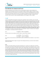
Caliper
A special type of ruler is the caliper. This device is equipped with a “beak” with two “jaws”. One of the
jaws is fixed to a ruler, while the other can slide along the ruler. It is therefore an ideal instrument to
measure the size of rectangular and round objects. The object is put in between the jaws, the beak is
closed around the object and then the measured value can be read. Usually, the jaws are made such that
the caliper can measure inner size and outer size of objects, as indicated by (1) and (2) in Figure 1. Also, a
depth gauge is usually present, so that the for example the depth of a groove or a hole can be measured.
The way this is done is displayed at (3) in Figure 1.
Figure 1: different measurement methods with the caliper (source: craftsmanspace.com)
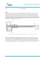
The accuracy of measurements made with the caliper depends again on the spacing of the tick marks.
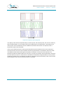
However, usually the caliper is equipped with two scales: a fine one and a coarse one. Normally, the
coarse scale has a 1 mm spacing between the marks, and the fine one has a spacing of 0.9 mm. Such
caliper is called a Vernier caliper. The scale is read at the point where the coarse and fine scale tick marks
coincide, as indicated in Figure 2. In this way, measurements with ±0.05 mm accuracy can be made.
Additional technical information for CanSat competition 2014
Reference: CSUK-T01
Version: 2.0
Page 11/53
Figure 2: Vernier caliper indicating a length of 11.4 mm (courtesy of T-Minus)
Angles
A second quantity that is important in defining the geometry of objects is the angle. The angle between
two lines defines the orientation of one line with respect to the other. Angles can be expressed in two
types of units: degrees (deg or 0) and radians (rad). The translation from degrees to radians and back is
done via expression 1.4.
(0.4)
Angle [ deg ] =
180
π
× Angle [ rad ]
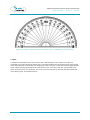
Protractor
The most widely used tool to measure angles is called the protractor. A picture of such device is
displayed in Figure 3. It consists of a scale in the shape of a half circle, with tick marks at equal distances
along the rim. The angle of a certain corner is measured by aligning the straight edge of the half circle
with its first side, with the center mark of the circle (usually the zero mark) at the corner itself. The angle
is then measured by determining which tick mark is coinciding with the second side. The accuracy of the
protractor depends on the spacing of the tick marks, just as for the ruler. If the tick marks are spaced with
1 degree angles, the measurement has an accuracy of ±0.5 deg.
Additional technical information for CanSat competition 2014
Reference: CSUK-T01
Version: 2.0
Page 12/53
Figure 3: schematic representation of a protractor (source: math8geometry.wikispaces.com)
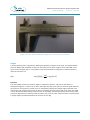
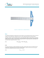
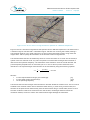
T-square
A tool that is frequently used to draw corners with a defined angle is the T-square. This device is
composed of two parts: the block and the ruler. The angle between the ruler and the block may be fixed
at any angle between 0 and 90 deg. For drawing the corner, the ruler is fixed at the desired angle and the
block is placed in alignment with the first side of the corner. The base of the ruler is positioned at the
place where the corner is to be drawn. The corner can then be drawn by following the edge of the ruler
with a drawing tool, for example a pencil.
Additional technical information for CanSat competition 2014
Reference: CSUK-T01
Version: 2.0
Page 13/53
Figure 4: A T-square (source: mathasteward.com)
Mass
The quantities that define the shape and size of an object are now discussed. However, there is one more
property of the CanSat that is important to know: its mass. Determining the mass of the CanSat is
necessary in order to size the parachute, and to verify if the design meets the requirements. Just like the
quantity length, the mass can be expressed in metric and imperial units. Metric units are for example the
kilogram (kg) or the gram (g), while the mass in imperial units is normally expressed in pounds (lb). The
conversion from kilogram to pounds is done by:
(0.5)
Mass [ kg ] = 2.205 × Mass [ lb]
Scale
The mass of an object is normally measured with a scale. A simple scale consists of a suspension hook,
connected to a calibrated spring and a pointer. When an object is placed on the hook, the spring will
extend with a length proportional to the mass of the object:
(0.6)
ΔLspring = n ⋅ M
Additional technical information for CanSat competition 2014
Reference: CSUK-T01
Version: 2.0
Page 14/53
Where
•
•
•
•
•
Δ indicates a difference, or change of the quantity following it
L denotes the spring length
Spring means that the length of the spring is meant
M is the mass of the object placed on the lever
n expresses how much the lever will extend at a given mass
[-]
[m]
[-]
[kg]
[m/kg]
The amount of displacement can be read from the position of the pointer.
In most scales, there is an option included to “tare” the scale. This means that the position of the pointer
is manually adjusted such that it points to zero when no mass is put on the lever. This is convenient when
one wants to measure objects that have to be put in a container, for example sand. First, the container is
placed on the scale. Since the container has a certain mass, the pointer will indicate that a mass is placed
on the scale. The pointer position is then manually re-adjusted to zero, after which the sand is poured in
the container. Now, the pointer indicates only the mass of the sand.
Today, most scales are electronic. The spring consists of a piece of material of which the elasticity, or the
factor n in formula 1.6, is well determined, for example steel. The amount of extension of the material’s
length is measured with an electronic device: a sensor. The internal electronic system monitors the
sensor’s output and display the right value on a display. The “tare” function is completely integrated in
the software of the electronic system.
Electronics: voltage, current, resistance
The core of the CanSat is an electronic system, consisting of a microcontroller, electrical power source,
sensors and actuators. Electronic systems essentially consist of flowing electrons through conductors.
Each electron has a negative charge, expressed in the unit coulomb. Since electrons are flowing through
the conductor, charge is transported from one side of the conductor to the other. This transport of charge
is called current. It is expressed in coulombs per second, or amperes. In order to make the electrons flow
from one side to the other, a difference in potential, called a voltage, expressed in the unit Volt, is needed,
which essentially means that electrons want to leave, or are repelled, from one side and attracted to the
other. The higher the potential difference, the faster the electrons will flow and thus the higher the
current will be. This is expressed in Ohm’s law:
I=
(0.7)
U
R
where:
•
•
•
I is the current through the conductor
U is the voltage over the conductor
R is the resistance of the conductor
[Ampere, A]
[Volt, V]
[Ohm, Ω]
The resistance is essentially a figure that expresses how hard it is for electrons to flow through the
conductor. A high resistance means that a high potential is needed in order to achieve a certain current.
The resistance of a conductor depends amongst others on the material that the conductor is made of, the
size of the conductor (length, cross-sectional area) and the temperature.
Additional technical information for CanSat competition 2014
Reference: CSUK-T01
Version: 2.0
Page 15/53
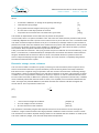
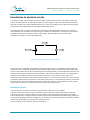
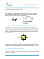
Multimeter
An easy device to measure the electronic quantities is the multimeter. It consists of an electronic
measurement unit and two measurement probes. A selection knob is used to choose which quantity is
measured, and in which range. Measuring the properties at a certain electronic component is quite easy,
but it has to be done in the proper way. The voltage over a component is measured by placing the
multimeter in parallel with it, indicated by (1) in Figure 5. When the selection knob is set to “voltage”, the
display will show the potential difference between the two measurement probes.
Current is measured by placing the multimeter in series with the conductor, as indicated by (2) in Figure
5. In this setup, the flow of electrons through both the conductor and the multimeter will be equal.
Therefore, when the selection knob is set to “current”, the display will show the amperes flowing through
the conductor. Finally, the resistance of a conductor can be measured. To do this, it is required that the
measured object is isolated from the rest of the electronic circuit, in order to avoid interference of the
other electronic components. The multimeter is now placed in parallel with the object and the selection
knob is set to “resistance”, as indicated by (3) in Figure 5. It now puts a well-defined voltage over the
probes and the object, and measures the current that flows. With Ohm’s law, the resistance of the object
can now be determined.
Figure 5: schematics of a multimeter
Additional technical information for CanSat competition 2014
Reference: CSUK-T01
Version: 2.0
Page 16/53
Example of CanSat setup with the European CanSat kit
There are of course numerous ways to construct your CanSat. The construction is limited by certain
constrains set by the organization (such as mass and size/volume constrains). But apart from those, the
engineering is only limited by your imagination and your building capabilities. Try to make a baseline
which is efficient, but still all parts are easily accessible. This way you have a fair amount of available
space in your CanSat for your secondary mission, but still you can easily switch part on site in case of
emergency.
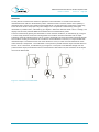
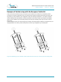
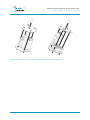
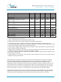
Some examples of how you could arrange your CanSat, with the European CanSat kit prototype 2013, are
displayed below. Of course you are totally free to choose any arrangement you would prefer.
Figure 6: Depending on your desired volume under the MCU board, you can store your 9V battery there
Additional technical information for CanSat competition 2014
Reference: CSUK-T01
Figure 7: alternative ways to arrange your MCU and sensor board and transmitter
Version: 2.0
Page 17/53
Additional technical information for CanSat competition 2014
Reference: CSUK-T01
Version: 2.0
Page 18/53
Parachute design and construction
In order to slow down your CanSat, you will need some sort of device that helps it to land. This can be
done in numerous ways, but two types of recovery mechanisms are highlighted in this chapter:
•
•
A drag device
A lift device
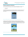
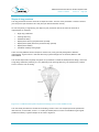
The drag device is by far the simplest way of slowing the CanSat down: it creates drag in order to reduce
the speed of a falling object. The most commonly known drag device is a parachute. A parachute is a
piece of fabric and cables, which create enough aerodynamic drag to slow the object down to a lower
descent velocity
Figure 8: a simple parachute, as used to slow humans down from a drop (source USMC)
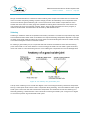
A lift device is much more complex than a drag device. It is basically a system which creates lift by
moving through the air. The air moves over and under the cleverly shaped lifting surface, resulting in a
large lifting force and a small drag force. A good example of a lift device would be an aircraft wing or ram
air parachute. The big advantage of this type of parachute is that it is potentially steerable, when trimmed
correctly. The disadvantage is that they are highly complex to build, difficult to trim and are less reliable
in deploying correctly in the air.
Figure 9: a ram-air parachute, as modern parachutists use (source USMC)
Additional technical information for CanSat competition 2014
Reference: CSUK-T01
Version: 2.0
Page 19/53
The physics behind the drag parachute
The physics behind the drag parachute and the lift parachute are similar in nature. The formula’s
connected to the drag parachute are:
=1 2
Where:
•
•
•
•
•
Fdrag is the drag force from the parachute
ρ is the density of air
V is the airspeed of the parachute
Cd is the drag coefficient
S is the surface area of the parachute
[N]
[kg/m3]
[m/s]
[-]
[m2]
The cd, or drag coefficient, is a dimensionless number which depends on the shape of an object. Basically it
is a number that indicates how “easy” air, or any other fluid, is flowing around a shape. If the object is
very aerodynamic, like for instance an airplane or a car, this number is fairly low (for example 0.2). If the
shape is not so aerodynamic, such as a simple plate or a parachute shape, the Cd will be very high, for
example (0.8 or higher).
Of course these numbers are empirical and based on a certain area where this drag coefficient is
calculated over.
For a normal circular parachute the drag coefficient will be in the range of 0.75 over the flat surface of a
parachute. The flat surface of a parachute is the surface area when you put a parachute flat on a table
top.
The density of dry air can be calculated using the Ideal gas law
=
∙
Where:
•
•
•
•
ρ is the air density
p is absolute pressure
Rspecific is the specific gas constant for dry air
The specific gas constant for normal dry air is 287.058
[kg/m3]
[Pa]
T is absolute temperature at that altitude.
[K]
[J/(kg·K)]
Under normal circumstances the air density at sea level (15°C) is approximately 1.225 kg/m3.
The temperature at altitude depends of course on the weather and the ground temperature. As a general
rule it can be stated that in the troposphere, the lower layer of the atmosphere, the air temperature
decreases with approximately 6.5 K per kilometer.
Additional technical information for CanSat competition 2014
Reference: CSUK-T01
Version: 2.0
Page 20/53
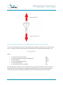
Figure 10: constant descent velocity: an equilibrium between forces (courtesy of T-Minus)
In case of constant descent velocity it can be stated that the weight of the drop mass (or CanSat in this
case) + parachute is equal to the drag force of the parachute. This means that the following is true:
=1 2
Where:
•
•
•
•
•
•
m is the mass of the total system
g is the gravitational acceleration of 9.80665 m/s2
ρ is the air density
V is the airspeed of the parachute
cd is the drag coefficient
S is the surface area of the parachute
[kg]
[m/s2]
[kg/m3]
[m/s]
[-]
[m2]
By combining these formulas, we can calculate how big the parachute should be in order to have the
desired descent time. Furthermore, by dimensioning the parachute, you can also predict the impact
velocity of your CanSat, by taking the air density ρ as the value of ISA sea-level of 1.225 kg/m3.
Additional technical information for CanSat competition 2014
Reference: CSUK-T01
Version: 2.0
Page 21/53
Shapes of drag parachute
The drag parachute can have all kinds of shapes and sizes. The size of the parachute is a direct result of
your drop-mass (the CanSat in this case) and your desired descent velocity.
As with everything in engineering, the shape of your parachute will be the result of all kinds of
requirements, for example:
•
•
•
•
•
•
•
High drag coefficient
Packing efficiency
Manufacturability
Deployment velocity (airspeed when opened)
Deployment speed (time from packed to fully opened)
Deployment stability
Pendulum stability during flight
There are many different kind of shapes to choose from, many specially designed for different
requirements. A good source is the book: Recovery System Design from Th. Knacke, ISBN-13: 9780915516858.
The normal shape that everybody recognises as a parachute is called the hemispherical design, which has
a high drag coefficient (meaning it is very efficient), a fair packing efficiency, but is difficult to produce,
since it involves a lot of sewing.
Figure 11: a traditional hemispherical parachute design (source www.madehow.com).
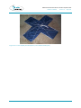
The most used parachute for CanSats and sounding rockets is the cross-shaped parachute (sometimes
referred to as cross formed-, X form- or crucifix-parachute) due to its ease in manufacturing and good
pendulum stability. A good example can be seen in Figure 12.
Additional technical information for CanSat competition 2014
Reference: CSUK-T01
Figure 12: A cross shaped parachute(source, www.nakka-rocketry.net)
Version: 2.0
Page 22/53
Additional technical information for CanSat competition 2014
Reference: CSUK-T01
Version: 2.0
Page 23/53
Lifting parachute
A lifting parachute is a much more complex device than a normal drag parachute. The device is basically
the same as an airplane wing but instead of being a rigid structure, it is inflated into its correct shape by
the incoming air. The wing will generate lift by the air which is flowing around it. A small added problem
with this lift is that it will come at a small price, namely drag.
A lot of formulas that describe the behavior of a lifting parachute go way further then the scope of this
CanSat project and go deep into aerospace engineering. The most important factor is the ratio between
lift and drag. This ratio, which is for simple lifting ram-air parachutes around 3 to 5, is also known as the
glide ratio. Basically this corresponds with the amount of horizontal distance can be obtained per vertical
distance.
Figure 13: the difference between a high glide ratio and a low glide ratio (courtesy of T-Minus)
In order to steer with a lifting parachute, some steering-lines can be attached to the leading edge of each
side of the wing. When one of these lines is pulled inwards, the wing has more drag on that side than on
the other side of the wing. This difference in drag can be used to steer the wing into the proper direction.
If the parachute is not properly trimmed, the wing can stall. This means that the wing will stop flying,
because the air not smoothly flowing around the wing anymore. Try to trim the wing forward again in
order to reduce this stall tendency.
It must be noted again that this type of parachute is definitely not recommended for beginners and is
very difficult to produce, deploy and fly.
Additional technical information for CanSat competition 2014
Reference: CSUK-T01
Version: 2.0
Page 24/53
Figure 14: a cansat with a ram air lifting parachute (source Miyazaki Laboratory)
Testing your parachute
A parachute is very easy to test. You can go to a high building where you have permission to drop
something small from (with such permission for instance your school building). Measure the drop height
in meters before you start. It is good to have a person with a video-camera standby to film all your tests
for later analysis. First throw your CanSat in a horizontal fashion to check if the deployment of the
parachute is according to your desires. Then throw your CanSat under an angle upwards, so that the
descent velocity is stable when it goes through the thrower’s horizontal. If you look later on the movie of
your test, you will be able to determine the time that the parachute spent descending from that point
until it touches the ground. Simple calculation can prove then what the average descent speed in
meters/second is. Try to do these kinds of simple tests a couple of times and average your results for best
accuracy.
Additional technical information for CanSat competition 2014
Reference: CSUK-T01
Version: 2.0
Page 25/53
Introduction to electrical circuits
To build the CanSat, you as a team will need to make a small electrical circuit. The system used for the
primary CanSat mission is provided, but it needs to be put together. There are many possible secondary
missions of which most require additional electrical circuits. This chapter will provide a short description
of electrical circuits and the basics of designing and building them.
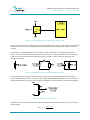
An electrical circuit is a network of electrical components, designed to fulfill a specific task. There are
many different sorts of electrical circuits, like your computer or a telephone. More simple circuits are for
example the light above the dinner table or a flash light. The flash light circuit contains three
components: a battery, a switch and a light bulb.
Figure 15: schematic diagram of a flash light
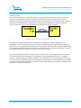
Figure 15 shows a schematic representation of the flash light circuit. In a schematic circuit diagram the
components are represented by symbols. Many different components have a dedicated symbol but there
are also components that do not. The meaning of the symbols depends on the system used. There are two
widely used systems: the American and the European. The reason symbols are used in circuit diagrams is
to make it more readable. Search on the internet for “Electrical circuit symbols” to find more. The
components are connected to each other by electrical wires. In an electrical circuit the wires are normally
not called components but connections. In the above picture they are represented by the lines connecting
the components. These lines indicate an electrical connection with very low resistance. In most systems
copper wire is used for the connection but other options are possible as well.
Reading of a circuit
In properly drawn schematics, there are three methods to make the circuit readable.
The first is reading from left to right. This means inputs are placed on the left side of the circuit and
outputs on the right. In the flash light circuit, the battery is the input and the light bulb is the output.
The second method is working from top to bottom. For electrical schematics this means high voltages are
on the top of the diagram and low voltages are on the bottom. The positive supply of the battery is drawn
at the top and indicated by the longer line and the plus sign.
The last method is the method to draw the connections.
Additional technical information for CanSat competition 2014
Reference: CSUK-T01
Version: 2.0
Page 26/53
Figure 16: schematic diagram of connected and not connected wires. The labelled wires are connected
In the simple schematic of the flash light there are only 3 connections in only one loop. The simplicity of
this circuit makes it very clear. In more complicated circuits there are many more connections. Figure 16
shows how to draw connected and unconnected crossings. The two lines are connected when they are
drawn with an offset, and not connected when they cross. The power lines in an electrical circuit are
normally connected to many components. To prevent the situation where the drawing is unreadable
because it would contain too many lines, simple labels are used. As shown in the Figure 17, all
connections with 3V are connected together. The same holds for the 0V connections. However, for the
flash light circuit, using only labels does not make the schematic more readable. Finding a balance
between labels and lines is dependent on many aspects and to the choice of the designer.
Figure 17: different schematic representation of the flash light. Using labels does not necessarily makes
the diagram more readable.
Components
There are many different electronic components available. The core of every CanSat is built up with a few
basic components. These components are:
•
•
•
•
A micro controller
A power supply
A transmitter
some sensors
Inthis manual, the T-Minus CanSat kit is used as reference. The same principles apply to other
components.
Additional technical information for CanSat competition 2014
Reference: CSUK-T01
Version: 2.0
Page 27/53
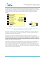
The micro controller is the main controlling and calculating component of the CanSat. There are many
manufacturers of micro controllers, which all make almost infinitely many different versions. All of these
controllers are based on a sequential processor, surrounded by several hardware interfaces. These
interfaces include systems like memory, analogue-to-digital converters and digital communication
systems.
U5A
10
11
12
13
14
15
5
6
19
20
21
22
23
24
25
PB0 (PCINT0/CLKO/ICP1)
PB1 (PCINT1/OC1A)
PB2 (PCINT2/SS/OC1B)
PB3 (PCINT3/OC2A/MOSI)
PB4 (PCINT4/MISO)
PB5 (SCK/PCINT5)
PB6 (PCINT6/XTAL1/TOSC1)
PB7 (PCINT7/XTAL2/TOSC2)
PC0 (ADC0/PCINT8)
PC1 (ADC1/PCINT9)
PC2 (ADC2/PCINT10)
PC3 (ADC3/PCINT11)
PC4 (ADC4/SDA/PCINT12)
PC5 (ADC5/SCL/PCINT13)
PC6 (RESET/PCINT14)
ATmega88PA
PD0 (RXD/PCINT16)
PD1 (TXD/PCINT17)
PD2 (INT0/PCINT18)
PD3 (PCINT19/OC2B/INT1)
PD4 (PCINT20/XCK/T0)
PD5 (PCINT21/OC0B/T1)
PD6 (PCINT22/OC0A/AIN0)
PD7 (PCINT23/AIN1)
26
27
28
1
2
7
8
9
U5B
3
16
17
VCC
GND
AVCC
GND
AREF
Thermal Pad
4
18
29
ATmega88PA
Figure 18 Schematic view of the ATmega88PA micro controller. The schematic is divided into an
input/output part (U5A) and a power supply part (U5B).
As the micro controller is a part that has many connections, sometimes up to 144 pins, discussing all
connections will not be part of this document. For the Atmel micro controller of Figure 18, there are 3
different types of inputs that will be discussed.
The first type of connection is the “general input/output” or GIO. In the Atmel micro controller all
input/output pins can be used in this manner. Connections starting with PB, PC, or PD are GIO pins. A GIO
pin can be used as input, where it will read a logical 0 or 1, depending on the voltage that is applied to it.
The GIO can also be set as output were the software determines if the pin is held high or low. If the pin is
held high then it will supply the same voltage as is being supplied at the VCC pin(s). When the GIO pin is
held low it will drain current to make supply 0V.
The second type of connection is the analogue-to-digital converter (ADC). Many micro controllers have
ADC’s on-board. These can be used to measure a voltage between 0V and the supply voltage. The
precision of the measurement depends on the amount of bits the ADC provides. Most ADC’s are 10 bit. A
10 bit ADC divides the voltage range in 210 = 1024 different steps, where 0 is the minimum value and
1023 is the maximum value. The ADC inputs of the micro controller can be recognised by the labels ADC0
to ADC5, for the micro controller of Figure 18
Additional technical information for CanSat competition 2014
Reference: CSUK-T01
Version: 2.0
Page 28/53
Figure 19 Basic principle of an ADC (source: wiki.ulcape.org)
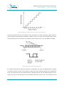
The last connection that will be discussed in this document is the UART connection. UART stands for
Universal Asynchronous Receiver/Transmitter. A UART connection is a basic serial communication system,
used by many devices. The com port of a computer uses the same protocol, only with different voltages.
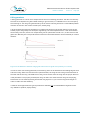
Figure 20 basics of UART communication
For a UART connection, the output of one device is connected to the input of a different device. In Figure
20 the basic protocol is shown. The connection is held high by the transmitter before the communication
starts. The transmitter starts the communication by making the line low for a predetermined time. This is
done to tell the receiver that data will be transmitted. After this start bit, one or several data bits are
Additional technical information for CanSat competition 2014
Reference: CSUK-T01
Version: 2.0
Page 29/53
transmitted. At the end of the transmission a stop bit is sent to make the line high again. Normally, 8 bits
or 1 byte is transmitted between a start and stop signal.
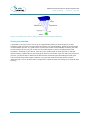
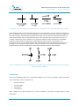
Sensors
The most basic sensors usually have an analogue output. An analogue sensor provides an analogue
voltage, depending on the measured quantity. For a pressure sensor, the air pressure is converted to
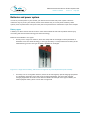
voltage. As an example, the MPX4115A pressure sensor will be used.
Figure 21: part of the datasheet from the MPX4115 pressure sensor (source Motorola)
The MPX4115A pressure sensor has 6 electrical contacts. The datasheet of the sensor describes the
function of each pin. As seen in Figure 21, pin 1 is Vout, pin 2 is GND, pin 3 is Vs the other pins are N/C or
“not connect” pins. For this component there is no predefined symbol, which means we have to make one
ourselves. Since there are only 3 connections used, the symbol will only contain 3 pins. Vout, or output
voltage, is an output, so it is placed on the right side of the symbol. GND is ground or negative power
supply and is placed at the bottom of the symbol. Vs, or supply voltage, is the positive power supply and
will be placed at the top.
Figure 22: self-made symbol for the MPX4115
To connect the pressure sensor it is important to understand some of its characteristics. The datasheet of
a component describes the operational characteristics. These describe properties like sensitivity, accuracy,
maximum and minimum operating voltages and current usage.
Table 2: characteristics sheet from the MPX4115 datasheet
Operating Characteristics
(VS = 5.1 Vdc, TA = 25°C unless otherwise noted, P1 > P2 Decoupling circuit shown in Figure 3 required to
meet electrical specifications.)
Additional technical information for CanSat competition 2014
Reference: CSUK-T01
Characteristic
Version: 2.0
Page 30/53
Symbol
Min
Typ
Max
Unit
Pressure Range(1)
Pop
15
-
115
kPa
Supply Voltage(2)
Vs
4.85
5.1
5.35
Vdc
Supply Current
Io
-
7
10
mAdc
Minimum Pressure Offset(3) (0 to 85°C)
@ VS = 5.1 Volts
Voff
0.135
0.204
0.273
Vdc
Full Scale Output(4) (0 to 85°C)
@ VS = 5.1 Volts
Vfso
4.725
4.794
4.863
Vdc
Full Scale Span(5) (0 to 85°C)
@ VS = 5.1 Volts
Vfss
-
4.59
-
Vdc
Accuracy(6) (0 to 85°C)
-
-
-
± 1.5
%Vfss
Sensitivity
V/P
-
46
-
mV/kPa
Response Time(7)
tR
-
1.0
-
ms
Output Source Current at Full Scale Output
Io+
-
0.1
-
mAdc
Warm-Up Time(8)
-
-
20
-
mSec
Offset Stability(9)
-
-
± 0.5
-
%Vfss
1. 1.0kPa (kiloPascal) equals 0.145 psi.
2. Device is ratiometric within this specified excitation range.
3. Offset (Voff) is defined as the output voltage at the minimum rated pressure.
4. Full Scale Output (VFSO) is defined as the output voltage at the maximum or full rated pressure.
5. Full Scale Span (VFSS) is defined as the algebraic difference between the output voltage at full rated
pressure and the output voltage at the minimum rated pressure.
6. Accuracy (error budget) consists of the following: Linearity, Temperature Hysteresis, Pressure Hysteresis,
TcSpan, TcOffset, Variation from Nominal
7. Response Time is defined as the time for the incremental change in the output to go from 10% to 90%
of its final value when subjected to a specified step change in pressure.
8. Warm-up is defined as the time required for the product to meet the specified output voltage after the
Pressure has been stabilized.
9. Offset stability is the product’s output deviation when subjected to 1000 hours of Pulsed Pressure,
Temperature Cycling with Bias Test.
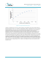
Starting at the top of the Table 2, the pressure range is the range of pressures the device can measure.
The supply voltage indicates the voltage required on the Vs pin in reference to the GND pin to use the
sensor. The board provided with the CanSat kit has a 5V power supply, which is within the range
indicated in the table. The supply current of this device is normally 7 mA with a maximum at 10 mA. This
current can be used in calculations on required power supply or the expected battery life. The next lines
describe how the Vout pin reacts to the applied pressure. This part will be required during calibration and
analysis of the signal. For this part it is important to note that the output is an analogue voltage.
Connecting the pressure sensor to a micro controller can be done in many different ways. Two things are
important in connecting this sensor: the power supply and the fact that the output is analogue. With the
output of the sensor being analogue it needs to be connected to an ADC of the micro controller.
Additional technical information for CanSat competition 2014
Reference: CSUK-T01
Version: 2.0
Page 31/53
Figure 23: schematic diagram of a connected pressure sensor
Figure 23 shows how this component is connected. The output of the sensor is connected to an ADC input
of the micro controller. The Vs and GND pins are connected to 5V and 0V the power supply used in this
example.
As example for a temperature sensor, a thermistor is used. A thermistor is a temperature dependent
resistor. To measure the temperature with a thermistor there are 2 basic possibilities: on can either put a
voltage across the thermistor and measure the current, or send a current trough the thermistor and
measure the voltage.
Figure 24: thermistor symbol and the measurement options.
The methods shown in Figure 24 either need a current source or current measurement. The simplest
current measurement is the use of a resistor with a fixed and predefined resistance, to convert current in
voltage. The drawback of this approach is that the calculation of the temperature becomes more difficult.
Figure 25: readout of the thermistor
Together with the resistor, the thermistor can be connected like the pressure sensor, in order to read the
output voltage.
∙ =
+
Additional technical information for CanSat competition 2014
Reference: CSUK-T01
=
∙ −
=
5 ∙ 10
Version: 2.0
Page 32/53
− 10
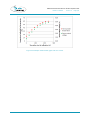
The above formula describes the relation between measured voltage and the resistance of the thermistor.
With this resistance the temperature can be calculated from the thermistor datasheet. The
NTCLE203E3103GB0 thermistor made by VISHAY BC Components is used to describe the basics of the
temperature measurement. This is a negative temperature coefficient thermistor, which means that the
resistance decreases with increasing temperature.
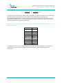
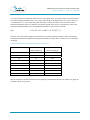
Table 3: part of the table describing the relation between temperature and resistance from the
thermistors datasheet
Temperature
resistance
°C
kΩ
0
32.56
5
25.34
10
19.87
15
15.70
20
12.49
25
10.00
30
8.059
35
6.535
40
5.330
The datasheet of the thermistor shows a table of the relation between temperature and resistance, of
which Table 3 is a part. Using this relation the acquired resistance can be calculated back in to
temperature.
Additional technical information for CanSat competition 2014
Reference: CSUK-T01
Version: 2.0
Page 33/53
Communication
The last part of an electric circuit that will be discussed is digital communication. There are two main
options for communication: serial or parallel. In this document, only serial communication will be
addressed. The serial communication method used by the CanSat kit as it is provided, is UART. With this
communication method there is a dedicated line connecting the transmitter of one device with the
receiver of the other. If two-way communication is required, two lines are needed.
Figure 26: schematic diagram of a UART connection
The UART line is made high and low by the transmitter, depending on whether a digital 0 or 1 is
transmitted. To receive this signal the receiver needs to read the line at the right moment to determine
whether a 0 or 1 is transmitted. The moment at which the status of the data line is read, is predetermined
by the speed at with the transmission is made. The transmitter sends a start bit to indicate the receiver to
start reading. Then the data byte is transmitted, followed by a stop bit.
One other common form of serial communication is via the I2C bus. I2C bus stands for Inter-Integrated
Circuit bus. The reason for calling this I2C instead of IIC is that mathematically I times I is I squared,
writing I^2. Officially the bus is called “I squared C (I2C)”, this became I2C to make it easier to write. The
I2C system uses two communication lines; one data line and one clock line. The advantage of this method
is that the communication speed does not need to be set on beforehand. Next to that, it is possible to get
feedback on communication quality.
Additional technical information for CanSat competition 2014
Reference: CSUK-T01
Version: 2.0
Page 34/53
Batteries and power system
In order to provide power to your CanSat, you need to have an electrical power system. There are
numerous ways to power your CanSat, but the most sensible way is to incorporate a battery. Other
options, such as photovoltaic cells (solar cells) can be explored but are outside the scope of this chapter.
Battery types
A battery is a device which consists of one or more electrochemical cells which produce electricity by
converting the stored chemical energy into electrical energy.
Batteries are available in two types:
• Primary cells or single-use batteries, which are cheap and can be bought in the supermarket or
hardware store. The chemical energy in this type of battery is incorporated in the battery at the
manufacturing process. This type of battery CANNOT be recharged.
Figure 27: a single use 9V battery, which can be bought at any local supermarket (source AFGA)
•
Secondary cells or rechargeable batteries, which can be recharged by special charging equipment.
It is absolutely necessary to use the proper charging equipment. The use of the improper
charging equipment can result in fire and toxic fumes. An example of this type of battery is a
lithium polymer battery which can be seen in Figure 28.
Additional technical information for CanSat competition 2014
Reference: CSUK-T01
Version: 2.0
Page 35/53
Figure 28: a lithium polymer battery, which is rechargeable with special balanced-charging equipment.
(source Wikimedia.org)
Advantages and disadvantages
The rechargeable battery has several advantages and disadvantages with respect to a single use battery.
It depends on the requirements you have on a battery which battery you will need for your CanSat.
Some considerations for choosing a battery type may be:
•
A rechargeable battery can obviously be recharged during the project, which could result in a cost
saving, because you do not need to buy new single-use batteries all the time.
•
The energy density of a rechargeable battery is higher than a single use battery. This means that
for example 100 grams of rechargeable battery can contain more energy than 100 grams of
single use battery. This is a very important factor in aerospace engineering, where every gram
counts!
•
The disadvantage of the rechargeable battery is that you will need special charging equipment to
charge your battery. This can be (very) expensive. Charging a battery can be dangerous, so always
charge your battery on a non-combustible surface and never let it be unsupervised.
•
Note: ALWAYS come to the launch site with fully charged batteries, or a fresh single use battery.
Calculations with a battery
The ESA CanSat kit needs voltages between 5.5V and 15V and has a power requirement of approximately
80 mA depending on the operation and the connected sensors.
When a device which needs 80 mA is connected to for example a battery of 550 mAh, this means that it
can run for
= 6.9ℎ
. Of course, this will just be a rough estimation, since other factors, like
resistance, current, battery internal resistance, battery temperature, etc. influence the actual battery
lifetime. In general, the battery output voltage will drop during the lifetime of the battery. This is highly
dependent on the amount of current that is consumed. Battery datasheets provide good reference for
several types of current loading.
Additional technical information for CanSat competition 2014
Reference: CSUK-T01
Version: 2.0
Page 36/53
The standard CanSat kit is powered by a simple single use 9V primary cell, of which specifications can be
found in Figure 29.
Battery tips and tricks
Having a good, stable and reliable voltage supply is absolutely essential for having a good and reliable
CanSat. The CanSat electronics will only work when they are supplied with enough power. If the voltage
drops only a fraction of a second under the 5.5V, strange things can happen, such as resetting
microcontrollers or loss of signal. Make sure that the battery of the CanSat is fixed properly in the CanSat
so that the battery leads are not momentarily disconnected when the rocket is accelerating, or the
parachute is deployed with a high shock.
Another thing that could happen is that some subsystems of your CanSat (momentarily) use a lot of
power. Due to this high power consumption, the voltage that the battery supplies to the system drops,
which can result for instance in a reset of one or more microcontrollers.
Additional technical information for CanSat competition 2014
Reference: CSUK-T01
Version: 2.0
Page 37/53
Figure 29: typical datasheet of a zinc –manganese-dioxide battery, which is supplied by the kit. (source
AFGA)
It is definitely not recommended to use the provided battery for flight. It is a simple test-battery to be
used just for that: testing the CanSat on the ground.
Additional technical information for CanSat competition 2014
Reference: CSUK-T01
Version: 2.0
Page 38/53
Introduction to soldering and circuit assembly
With a schematic diagram of an electric circuit completed it is time to go from theory to practice. To build
an electric circuit, you need the components and a printed circuit board (PCB) to place them on. The PCB
can either be one especially made for your circuit, or a general PCB on which you make the connections
of your circuit yourself. This chapter will first show some component placement and connection methods
for nonspecific PCB’s. The design of custom made PCB’s is not part of this document, although some
possible advantages will be addressed. The last part of this chapter will provide a short introduction and
checking method for soldering of the components.
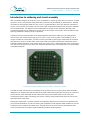
A general form of nonspecific PCB’s is the experimentation PCB with a solder grid. The most general
version has a grid of holes with a spacing of 2.54 mm, or 100 mil. Every hole is surrounded by a bit of
copper to solder the components. A circuit is built on such PCB by placing the components on the board
and then using wires to connect them. These wires need to be placed such that the connections of the
schematic diagram and built circuit are the same. Using short wires is better than long wires. The longer a
wire, the more resistance it has. If the wire resistance becomes high it will influence the circuit and result
in unwanted behavior.
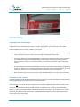
Figure 30: an empty CanSat kit sensor board (courtesy of T-Minus)
The PCB provided with the kit for the building of the primary mission is a semi-specific PCB. The PCB is
designed in the shape of the main board with the solder-able holes aligned such that they can connect to
the connectors of the main PCB. All the connections that go to the main board have an extra hole
connected to them to make connecting wires easier. Looking closely at the board, the lines can be seen
that make these connections.
Placing the components is a puzzle wherein the complexity depends on the amount of components and
your personal demands on circuit size. Placing the components close together makes it harder to wire the
connections, but it requires less board space. Leaving room for the wires will ease the soldering later
while it increases the board space required. Building a PCB is planning ahead.
Additional technical information for CanSat competition 2014
Reference: CSUK-T01
Version: 2.0
Page 39/53
Design of a dedicated PCB is a method to make soldering much simpler and creates less of a hassle with
wires to connect everything. Making a specific design provides more flexibility in the components that
can be used. On the general PCB the grid is 2.54 mm, but most of the modern components are much
smaller than that. There are many programs available for making PCB’s. One that has a free license for
non-commercial use is the computer program “Eagle”. After the PCB is designed in such a program, it
needs to be fabricated. This fabrication can be done by dedicated factories.
Soldering
Soldering is needed to make the components electrically connected. To solder the components they need
to be heated and then solder needs to be added. The required soldering temperature depends on the type
of solder used. Solder made for electrical circuits melts at around 183 degrees Celsius for leaded versions,
or around 230 degrees Celsius for lead-free solders.
For making a good solder joint, it is important that both surfaces are heated to more than the melting
point of the solder. If one of the surfaces is not hot enough, the solder will not make a good connection,
which will result in a non functioning electric circuit. Making the components too hot will damage them.
Figure 31: the anatomy of a good solder joint
The tip of the soldering iron is around 350 degrees. This is hot enough to destroy almost all components.
Luckily, it takes quite some time to break a component during soldering. The time needed to make a good
solder joint is much less then the time that the components can sustain the heat of the soldering iron.
Generally speaking, it takes between 1 and 2 seconds to make a good solder joint. In Figure 31 to Figure
32 are several pictures of good and bad solder joints
Additional technical information for CanSat competition 2014
Reference: CSUK-T01
Figure 32: drawing of good and bad solder joint
Figure 33: photographs of bad soldering (courtesy of T-Minus)
Version: 2.0
Page 40/53
Additional technical information for CanSat competition 2014
Reference: CSUK-T01
Figure 34: photographs of good soldering (courtesy of T-Minus)
Version: 2.0
Page 41/53
Additional technical information for CanSat competition 2014
Reference: CSUK-T01
Version: 2.0
Page 42/53
Radio communication
Radio communication is sending information from one place to another, using electromagnetic waves,
also called radio waves. Electromagnetic waves are generated at an antenna when an alternating electric
current is connected to it. The antenna transforms the electric current is electromagnetic waves. At the
receiving end of the communication, the waves are transformed back into electric current by an antenna.
Using the radio waves to transfer information means that the information needs to be added to the radio
frequency used. Adding this information is called modulation and can be obtained in several ways. The
most basic form is to transmit a (carrier) frequency or not. This is called continuous wave (CW)
communication. The most used form of CW is Morse code. The biggest drawback of this is that the
information transfer rate or baud rate is very low.
There are many other forms of modulation, such as AM and FM. These are used by radio stations. With AM
(amplitude modulation), the information is made to change the amplitude of the carrier frequency. In FM
(frequency modulation), the frequency of the carrier is changed, as depicted in Figure 35. The advantage of
FM over AM is that the signal strength does not interfere with reception.
Figure 35: the difference between AM and FM modulation
The CanSat kit has a transmitter that modulates with Frequency Shift Keying (FSK). This means that it is
transmitting a frequency when a logic 0 is transmitted and a different frequency if a logic 1 is
transmitted, as depicted in Figure 36. There are many other forms of modulation like QPSK where two
bits are transmitted simultaneously.
Additional technical information for CanSat competition 2014
Reference: CSUK-T01
Version: 2.0
Page 43/53
Figure 36: frequency shift keying FSK
The quality of the radio link depends mainly on three aspects: the transmit power, the receiver sensitivity
and the used antennas. The only aspect that can be influenced by the CanSat team is the antenna. The
other aspects can be influenced, but then a different transmitter and receiver are required, which is
beyond the scope of this document.
There are two antennas used in receiving the information from the CanSat: the first is the antenna on
board the CanSat, the second is the antenna used at the ground station. The antennas need to be made
with different requirements, although the frequency of operation is similar for both antennas. The
antenna on board the CanSat needs to be isotropic (or as much as possible), which means that it transmits
the same amount of power in all directions. The antenna connected to the ground station can be pointed
towards the CanSat, and it can therefore be made as a high-gain directional antenna, which receives more
electromagnetic waves from one direction then from another.
Additional technical information for CanSat competition 2014
Reference: CSUK-T01
Version: 2.0
Page 44/53
Figure 37: an “Arrow” which is a Yagi antenna for operation at 2 different frequencies
Figure 37 shows a directional Yagi antenna that operates at two different frequencies. The antenna has a
7 elements Yagi for 433 MHz and a 3 elements Yagi for 145 MHz. For receiving the CanSat, building a
Yagi antenna might be a very good option since it can be constructed relative easily, using wood and
copper tubes. There is plenty of information on the internet to build a Yagi antenna.
The CanSat antenna needs to be sufficiently robust to survive the launch on a rocket. For the CanSat, a
quarter-wave wire antenna works very well. The quarter-wave describes the length of the antenna in
reference to the operation frequency. The transmitter of the CanSat kit works at around 434 MHz. the
precise frequency depends a bit on what team you are in. This is done to protect each other from
interference. The required length of the antenna can be calculated by using the following equation
=
4
=
3 ∙ 10
4 ∙ 434 ∙ 10
Wherein:
• L is the required antenna length (1/4 wavelength)
• C is the speed of light (300.000 km/s)
• f is the operating frequency
= 0.173
[m]
[m/s]
[Hz]
The formula shows that the length of the antenna for 434 MHz should be around 17.3cm. The wire can be
soldered to the antenna contact of the transmitter board directly, or, when using a coaxial cable, the
antenna can be placed some distance away from the board. When using a coaxial cable, the last 17.3cm
the outer conductor needs to be removed to form the actual ¼ wavelength antenna. Protect the
insulation material, as electric contact with metal surfaces might damage the transmitter.
Additional technical information for CanSat competition 2014
Reference: CSUK-T01
Version: 2.0
Page 45/53
Introduction to programming
There are many forms of programs, such as computer programs, websites, mobile phone apps and many
more. These programs are used for many different applications from, running your microwave oven to
allowing you to check your bank account on the internet. All programs have one thing in common: they
are written using a programming syntax. This syntax is often called the programming language. The
syntax is a method to describe what the program needs to do. Depending on the application, a program
either needs to be compiled before use or it is compiled while using the program. Most webpages use
languages that allow the web browser to compile or read the programming language directly. Languages
that can be used for this are HTML or JAVA. Computer programs need to be compiled before use to
change the program syntax in to instructions that the computer understands.
Every (Computer) processor has an instruction set of binary codes used by the processor to undertake
certain actions. This type of programming is used during the CanSat competition. The micro controller
provided in the CanSat kit is a small computer. Micro controllers are used in many systems, like robot
welding machines. The difference between a micro controller and the processor in your computer is that
a controller is a processor with hardware control and memory in one component. During the CanSat
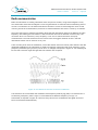
competition the C programming language will be used and Arduino will be used as compiler.
1.
int function ( char a )
2.
{
3.
char b, C;
4.
int Data = 10;
5.
6.
// comment
7.
b = a + Data;
8.
C = b – 1;
9.
Anotherfunction( C );
10.
return b;
11.
{
Above, a short example of a program written in C is given. To describe the entire language in this
document will not be possible and also not useful. This is mainly because Arduino uses several libraries
to make life simple. Therefore this document will describe the bare minimum, while more information
can be found on the Arduino website or more general all over the World Wide Web. Many examples can
also be found in the Arduino program.
Additional technical information for CanSat competition 2014
Reference: CSUK-T01
Version: 2.0
Page 46/53
The programming language can mainly be separated in 4 groups: functions, variables, operations and
formatting.
• Functions are bits of code that do several tasks. Functions can be premade or user made. A
function is “called” during the program if the task it is made for is required.
• Variables, as the name implies, are used to store values that might change during the program. A
variable in C needs to be defined at the beginning of a function (local variable) or before the first
function (global variable). There are several types of variables, depending on the size they have.
• Operations determine what happens in the program, such as adding two variables. Operations can
also compare variables to go through certain code only in certain situations.
• Formatting is required for the computer to understand what you want. Some of the formatting is
also used to make a program more readable for users. Two of the (many) formatting aspects are
the semicolon (“ ; ”), which is used to end most of the programing lines, indicating to the
computer that the statement before must be done before continuing. The “// ” this tells the
computer that everything behind the “ // “ and on the same line is comment, this is used to
explain certain pieces of code.
Using the short example above lets describe what an operation is. The program shown is a function
called “function”. If program calls “function” line 1 tells how this function is called. In this case the
function is defined as an integer (int). This means that the function will return a 16 bit value when
finished. One often used definition is “void” if no return value is needed. The second part of line 1 defines
the value that is given to this function when called. Here the function needs a character, or 8 bit value,
which is then placed in variable “a”.
The “char a” and “char b, C” parts of line 1 and 3 are the definition of local variables. These variables can
be used inside this function and will be forgotten by the program when this function is left. Line 3 defines
two values as “char” without any starting value. Line 4 defines the variable “Data” with a value of 10 to
start with.
Lines 2 and 11 define where the function “function” begins and ends with the brackets ‘{‘ and ‘}’. By using
a tab with the lines in between it is very clear where this function starts and where it ends. This also
makes it easier to see if the brackets are placed correctly. Line 5 is an empty line used to make the
program readable. Line 6 is a comment line used for the same purpose.
Lines 7 and 8 are operations, in this case small calculations to change variables. Line 9 is a call to the
function “anotherfunction” where the value of variable “C” is given to this function. Line 10 determines
what value the function “function” returns when finished.
Data inconsistencies
The above program has 2 problems with variables. The first one is on line 7. In this line, an integer and a
character are added together and the result is placed in a character. The problem is that the integer is 16
bits and this is placed in an 8 bit variable. So either b needs to be an integer or Data a character. The
second problem is that function returns an integer while the return line only provides a character. The
compiler will either provide a warning or error to indicate this mismatch.
Additional technical information for CanSat competition 2014
Reference: CSUK-T01
Version: 2.0
Page 47/53
Introduction to data analysis
At this point, you are at the stage where your CanSat is fully operational. You are able to perform
measurements with the sensors and your CanSat can send the measurement data down to your ground
station, where they are received. If everything went well, you received a stream of data lines. Each line
consists of a time mark, indicating when the measurement was taken, and some numeric values of the
voltages that your sensors recorded. From this data set, you want to deduce the actual quantities that
your sensors measured, such as pressure and temperature. Then you want to present these quantities in a
nice and clear way. This chapter provides you with guidelines on how to perform these steps.
From data to measurements: calibration
The data that are received so far do not provide good insight into the quantities that are actually
measured, such as air temperature: they are just voltages as obtained from the sensor outputs. To obtain
valuable measurements, the voltages will have to be converted into the measured quantity. This can be
done by determining a calibration curve for the sensor. A calibration curve essentially tells what output
voltage can be expected when the sensor is subjected to a given temperature. This means that the curve
can be used in the reversed way as well: it tells you what temperature the sensor senses when the output
voltage is a given value. Therefore, measurements can be deduced from the data with this curve.
In most cases, the relation between the sensed quantity and the output voltage is linear, which means
that it can be expressed as:
(0.8)
Qmeas = a ⋅Vout + b
Where
•
•
•
•
Qmeas is the value of the measured quantity (for example temperature)
Vout is the output voltage of the sensor
a is the calibration gradient
b is the calibration offset
[K]
[V]
[K/V]
[K]
Calibration of the sensor means therefore determining the values of a and b. For some sensors, this is very
easy: just check the data sheet of the sensor. The gradient and offset should be given here. However, in
most cases, only a range of values is given: the gradient and offset may be in between a certain minimum
and maximum value. Determining the exact values is therefore necessary.
The equipment needed to perform a calibration is a source of the quantity that is measured (for the
temperature sensor, this is a device that can give the sensor a given, well-defined temperature, for
example a glass with water on a hot plate), and a pre-calibrated sensor, such as a thermometer. The
thermometer and the sensor are both placed in the glass of water and the output from the sensor as well
as the indicated temperature on the thermometer is monitored and noted down. Now, the temperature of
the water is gradually increased by turning on the hot plate. At given time intervals, both the sensor
output and the reading from the thermometer are noted. The calibration can be stopped when 5 – 10
measurement within the desired range of temperatures are obtained. An example of the noted values is
given in Table 4.
Additional technical information for CanSat competition 2014
Reference: CSUK-T01
Version: 2.0
Page 48/53
Table 4: Example calibration curve measurements
Time of measurement [s]
Temperature of
Temperature sensor
thermometer [0C]
output voltage [V]
0
15
0.60
30
25
1.53
60
34
2.35
90
41
3.05
120
48
3.63
150
53
4.10
180
56
4.45
210
59
4.68
240
60
4.80
Now, the measurements are drawn into a graph, with the sensor voltage on the X-axis and the
temperature on the Y-axis. The points should form a more-or-less linear line, as indicated in Figure 38:
Example calibration curve. When this is done in a computer program, usually the possibility exists to add
a so-called “trend line”. This is a given function (linear, polynomial, exponential, etc.) of which the shape
parameters are automatically adjusted such that the best fit of the curve with the measurements is
obtained. In this case, a linear trend line is fitted, as indicated in Figure 38. The options “display equation
on chart” and “display R2 value on chart” are enabled. With the first option, the used formula is displayed,
while the second option shows the so-called R2- value. This value indicates how well the curve fits all the
measurement points. A value of 1 indicates a perfect fit, the lower the number, the worse the fit. One can
observe that the function of the linear fit has the same form as equation 1.8. This means that the values
of a and b can be read directly from the displayed function. In this case, they are 10.743 K/V and 8.6007 K
respectively. Now, the calibration curve is determined, and the actual data obtained from the CanSat can
be converted into real measurements, by applying equation 1.8.
Additional technical information for CanSat competition 2014
Reference: CSUK-T01
Version: 2.0
Page 49/53
Figure 38: Example calibration curve
Figure 39: Calibration curve with trend line
Results presentation
Now that the measurements are obtained, they have to presented in a clear and unambiguous way, so
that other people can understand them and the conclusions that are drawn from it. The most basic way to
present results is the table. An example is Table 5. The measured quantities are displayed in the columns,
while each measurement point is displayed in one of the rows. It is important that the columns are
labeled, so that it is clear what the meaning of the presented values is. The labels contain the quantity
(time, temperature and voltage, respectively), the object that has been measured (time, thermometer,
sensor) and the unit used to express the measured values (s, 0C, V).
A title or caption can be added to clarify the conditions in which the measurements were taken and how
they were obtained. Finally, the grid lines are displayed for readability.
Additional technical information for CanSat competition 2014
Reference: CSUK-T01
Version: 2.0
Page 50/53
It is important that the displayed values have the right significance. This means that if the measurements
of the thermometer are taken with 1 0C accuracy, they should be displayed with 1 0C accuracy, hence 15
0
C, instead of 15.0 0C. This is especially important when a certain conversion via a formula is used to
obtain the displayed value. If for instance, the output voltage of the sensor is read as being 3.63 V, and
the corresponding temperature is calculated with formula 1.9, the outcome would be:
T = 10.473 ⋅ 3.63 + 8.6007 = 47.59779 ⎡⎣ 0 C ⎤⎦
(0.9)
However, since the output voltage is measured with only three significant numbers, the corresponding
temperature should be rounded to three significant numbers as well, hence a value of 47.6 0C should be
displayed.
Table 5: Measurements of temperature sensor calibration 1
Time of measurement [s]
Temperature of
Temperature sensor
thermometer [ C]
output voltage [V]
0
15
0.60
30
25
1.53
60
34
2.35
90
41
3.05
120
48
3.63
150
53
4.10
180
56
4.45
210
59
4.68
240
60
4.80
0
Next to the table, a second convenient way of displaying measurement results is by means of a graph. An
example is given in Figure 40.
Additional technical information for CanSat competition 2014
Reference: CSUK-T01
Version: 2.0
Page 51/53
Figure 40: example measurement graph
A graph is composed by an X and Y-axis, with the values of one quantity at the X-axis and the values of
the second quantity on the Y-axis. Usually, the independent quantity is displayed on the X-axis, while the
dependent quantity is set on the Y-axis. It is important that the range of both axes is chosen wisely: all
measurements should be displayed and the entire graphing field should be used. If necessary, a
logarithmic scale can be chosen instead of a linear one, so that a wider range of measurements can be
displayed. Discrete (= not continuous) measurements should be displayed by a marker. If desired, the
markers can be connected by lines. Continuous functions may be indicated by a continuous line only. The
axes shall be labeled, just as the columns of a table, with measured quantity, object and unit. If more than
one data series is displayed, a legend should be provided, so that the series are easily distinguished. It is
important to remember that some colors, for example dark blue and red, are not easy to tell apart when
printed in black-and-white or grey shades. If the range of the one data series differs significantly from the
other, a second X or Y axis may be added for clarity, as visualized in Figure 41. Grid lines may be added to
the graph for easier reading. Finally, a title or caption can be added to provide more information on the
displayed values.
Additional technical information for CanSat competition 2014
Reference: CSUK-T01
Figure 41: Example measurement graph with two Y-axes
Version: 2.0
Page 52/53
Additional technical information for CanSat competition 2014
Reference: CSUK-T01
Version: 2.0
Page 53/53
Other resources and further information
http://upload.wikimedia.org/wikipedia/commons/0/07/Lithium_polymer_battery_%2811.1_volts%29.jpg
http://www.produktinfo.conrad.com/datenblaetter/650000-674999/650411-da-01-enAGFAPHOTO_9V_E_BLOCK.pdf
http://www.conrad.nl/ce/nl/product/650411/
http://upload.wikimedia.org/wikipedia/commons/e/e6/USMC_Paratrooper.jpg
http://en.wikipedia.org/wiki/File:Ram_air_square.jpg
http://forth.aero.cst.nihon-u.ac.jp/activity/e-a-pad.html
http://www.madehow.com/images/hpm_0000_0005_0_img0132.jpg
http://www.nakka-rocketry.net/xchute1.html