1
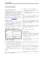
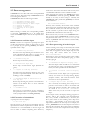
r.avalanche Version 2012-02-08 A model for simulating the motion of granular flows (debris flows and snow avalanches) based on GRASS GIS User manual and model outline by Martin Mergili Institute of Applied Geology, BOKU University of Natural Resources and Life Sciences Vienna, Austria [email protected] www.mergili.at February 2012 2 r.avalanche r.avalanche is a GIS-supported model framework for simulating the motion of granular flows like debris flows or snow avalanches over inclined surfaces. r.avalanche is designed as raster module for the software GRASS GIS. The scientific concepts behind r.avalanche are summarized in Chapter 1 (Model outline). In contrast to most of the other GRASS raster modules, management of the data and the parameters (input and output) is not done by adding parameters to the r.avalanche command, but by an additional shell script (r.avalanche.sh) with various functionalities, including input of data and parameters as well as post-processing and display of the results. Instructions how to operate the model framework are given in Chapter 2 (User’s manual). The model shows a large potential for refinements. Chapter 3 (Prospected improvements) will give a short overviev of ongoing and prospected further development of r.avalanche, regarding the scientific concepts behind it as well as its ease of use. Every user is encouraged to report encountered bugs or errors to [email protected]. Furthermore, the developer would be grateful for receiving comments regarding • experiences with the program, shortcomings, recommendations for improvements (scientific concepts, ease of use); • parameters chosen for certain study areas; • interest in cooperation with application and further development. The model, as applicable with GRASS, is running under the GNU General Public License (www.gnu.org). r.avalanche has been created with the purpose to be useful for modelling of debris flows. It has been developed with care, and much emphasis has been put on ensuring its scientific value. Nevertheless, every user has to be aware that it is only a computer program created by a human being, which may contain technical and topical errors and shortcomings. No responsibility can be taken by the developer for any types of deficiencies in the program or in this document, or for the consequences of such deficiencies. ___________________________________________________________________________ 1 Model outline 3 1.1 General aspects 3 1.2 Model layout 3 1.3 Implementation into GRASS GIS 4 1.3.1 Dimensionalization of the variables 4 1.3.2 Adaptation of the coordinate system 4 1.4 Acknowledgements 5 1.5 References 5 2 User’s manual 6 2.1 System requirements 6 2.2 Test dataset 6 2.3 File management 6 2.4 Installation 6 2.5 Data management 7 2.5.1 Parameter and data input 7 2.5.2 Execution of simulations 7 2.5.3 Post-processing of model output 7 2.5.4 Display of results 8 2.5.5 Removal of result files 8 2.5.6 Cleaning of file system 8 2.5.7 Exit 8 3 Prospected improvements 9 3.1 Scientific concepts 9 3.2 Ease of use 9 Model outline 3 1 Model outline 1.1 General aspects r.avalanche constitutes a fully deterministic model for the motion of granular flows (suitable for debris flows, flow avalanches, and other types of movements). The model builds on a solution of the Savage-Hutter (SH) model for simple concave topographies with an only vertically curved flow line, running out into a horizontal plane (Wang et al. 2004; Figure 1). This means that r.avalanche is only suitable for relatively simple terrain with straight channels. Future development, however, shall be directed towards overcoming this problem (compare Chapter 3). A curvilinear coordinate system is used instead of a simple rectangular system (compare Figure 1). where ζ is the downslope inclination angle of the reference surface, κ is the local curvature of the reference surface, b is the elevation above the reference surface, and ε and λ are factors (compare below). β x and β y are defined as β x = ε cos ςK x Eq. 6, β y = ε cos ςK y Eq. 7. K x and K y are the earth pressure coefficients in downslope and cross-slope directions. Eq. 8 top K y , act / pass = 1.2 Model layout r.avalanche requires far less input than r.debrisflow as it only simulates one part of the process. In contrast, the mathematical-technical concept behind r.avalanche is much more complex. A full description of the way how the SH model was solved for this specific topographic situation would go beyond the scope of this study – a detailed description is given by Wang et al. (2004). The most fundamental aspects are summarized below. Eq. 1 to 3 are the basis of the SH model: ∂h ∂ ∂ + (hu ) + (hv ) = 0 ∂t ∂x ∂y ) ( K x , act / pass = 2 1 1 − cos2 ϕ cos2 δ sec2 ϕ − 1 , Eq. 9 bottom 1 Kx +1 2 (K x − 1)2 + 4 tan 2 δ . φ is the angle of internal friction, and δ is the bed friction angle. Active stress rates (subscript act) are connected to dilatation of the material, passive stress rates are connected to compression – it depends on acceleration or deceleration of the flow whether active or passive stress rates are valid (compare Wang et al. 2004). Eq. 8 and 9 are only valid as long as the flow moves predominantly in downslope direction. z Eq. 1, y z0 2 ∂ (hu ) + ∂ hu 2 + ∂ (huv ) = hs x − ∂ β x h ∂t ∂x ∂y ∂x 2 ( ) , ζ y0 x0 Eq. 2 top Eq. 3 bottom x β h2 ∂ (hv ) + ∂ (huv ) + ∂ hv 2 = hs y − ∂ y . ∂t ∂x ∂y ∂y 2 ( ) h is the avalanche thickness, and u and v are the depth-averaged downslope and cross-slope velocities. s x and s y are the net driving accelerations: sx = sin ς − u u +v 2 Eq. 4 top sy = − u +v tan δ (cos ς + λκu 2 ) − ε cos ς ∂b , ∂x Eq. 5 bottom u 2 2 2 tan δ (cos ς + λκu 2 ) − ε cos ς ∂b , ∂y talweg Figure 1: The topography for which the solution of the SH model used in r.avalanche was elaborated (adapted from Wang et al. 2004) The system of equations described above is only valid for cohesionless and incompressible granular materials which can be considered as fluid continuum. It has to be emphasized that all variables are dimensionless, meaning that the model is scale-invariant and small-scale laboratory tests can be used as reference for large-scale problems in nature. The differential equations Eq. 1 to 3 were solved using a NOC (Non-Oscillatory Central Differencing) scheme, a numerical scheme useful to avoid unphysical numerical oscillations. Cell averages are computed 4 r.avalanche CFLx = max ∆xi alli , j CFLy = (β x )i , j hi , j ui , j + [ max vi , j + alli , j Eq. 10, (β ) h y i, j i, j ] ∆y Eq. 11, The implementation of the SH model and its solution by Wang et al. (2004) into GIS bears two problems: (1) the solution provides dimensionless values – in the GIS, however, it is necessary to use dimensional values; (2) the solution is valid for a curvilinear reference system only, in contrast to a GIS which usually uses a simple rectangular system. 1.3.1 Dimensionalization of the variables The first problem was solved using equations from Pudasaini (2003). They are based on the variables L, H, and R (compare Table 1). L is the typical avalanche length, H is the typical avalanche depth, and R is the typical radius of curvature (all in meters). Dimensional variables are derived using Eq. 16, Eq. 18, terrain surface reference surface z until z 0,test =z 0,terrain : z 0,test =x 0 *tan(90-ζ ) 90-ζ b y = Ly u = u gL t =t L g 2 45 increasing or decreasing x 0 x0 3 b =(x 0 ²+z 0,test ²) 1.3 Implementation into GRASS GIS Eq. 12, Eq. 14, z0 1 where ∆x and ∆y are the cell sizes in x and y direction and i and j are the coordinates of the cells in x and y direction, respectively. The length of one time step ∆t has to be smaller than 0.5 times the minimum from CFL x and CFL y . ∆t is determined dynamically while running r.avalanche, based on the CFL condition from the previous time step. Instead of 0.5, a factor of 0.2 was chosen in order to add some tolerance. x = Lx h = Lh v = v gL κ = Rκ where the variables denoted with a cap are the dimensional counterparts of the variables discussed above and g is gravitational acceleration (9.81 m s-2 on the earth surface). r.avalanche proved to work best when setting x, y, and h to the dimensional values (in m) while setting L, H, and R to 1. The factors ε = L/H and λ = L/R (Pudasaini 2003) were therefore 1. This contradicts the statement by Wang et al. (2004) that the factors should be far lower than 1, but appears appropriate when using dimensional values from the beginning with h being much smaller than the length of the flow. z0,test using a staggered grid, meaning that the system is moved half of the cell size with every time step (the values at the corners of the cells and in the middle of the cells are computed alternatively). The numerical scheme derived by Wang et al. (2004) was used for r.avalanche. The degree of diffusion of the flow material is governed by using slope limiters, restricting the gradients of flow depth to a certain range. The so-called minmod limiter has already been used by Wang et al. (2004) and also for the present study since it is known as the most diffusive one, reducing numerical oscillations. The simulation is run for a number of time steps until a certain break condition is fulfilled. The time steps have to be kept short enough to fulfil the CFL (Courant-Friedrichs-Levy) condition required for obtaining smooth solutions: Eq. 13, Eq. 15, Eq. 17, x step of iteration Figure 2: Iterative determination of b based on the coordinate system defined by the reference plane. Designed by M. Mergili. 1.3.2 Adaptation of the coordinate system The solution of Wang et al. (2004) builds on a curvilinear coordinate system based on a horizontally straight “talweg” which shall be the predominant flow direction. Three steps are performed for converting the original rectangular coordinate system in which the input raster maps are provided into the coordinate system for the simulation: (1) the coordinate system is rotated around the z axis so that the expected predominant flow direction derived from the starting material and the elevation model is aligned with the new x direction. This rotation is based on two userdefined pairs of coordinates in the flow channel (compare Table 1); (2) a reference surface is created, based on the defined “talweg” and an inclination of zero in y (cross-slope) direction; (3) based on this reference surface, the cell size ∆x for each x parallel to the reference surface is computed. The elevation b (m) – defined as the distance between terrain surface and reference surface perpendicular to the reference surface – is derived. This has to be done iteratively, varying the horizontal shift until the tested value of b converges with terrain height (Figure 2). After completing the calculation, the entire system is reconverted into the rectangular coordinate system Model outline 5 used in the current GRASS GIS mapset in order to enable a proper display of the results. 1.4 Acknowledgements Funding was provided by the Tyrolean Science Funds, the Vice Rector for Research of the University of Innsbruck (“Doktoratsstipendium aus der Nachwuchsförderung der LFU”), and the Austrian Academy of Sciences. Furthermore, the valuable remarks of Wolfgang Fellin (Institute of Infrastructure, University of Innsbruck), Katharina Schratz, and Alexander Ostermann (Institute of Mathematics, University of Innsbruck) are acknowledged. 1.5 References Pudasaini, S.P. 2003: Dynamics of Flow Avalanches Over Curved and Twisted Channels. Theory, Numerics and Experimental Validation. Dissertation at the Technical University of Darmstadt, Germany. 200 pp. Wang, Y.; Hutter, K.; Pudasaini, S.P. (2004): The Savage-Hutter theory: A system of partial differential equations for avalanche flows of snow, debris, and mud. ZAMM - Journal of Applied Mathematics and Mechanics / Zeitschrift für Angewandte Mathematik und Mechanik 84:507-527 Table 1: Input information required for running r.avalanche. map/parameter catchment elev delta riskobj dinit phi L H R deltatout tmax vmin xchan1, ychan1 xchan2, ychan2 symbol (unit) – (boolean) z (m) δ (degree) – (boolean) h 0 (m) φ (degree) L (m) H (m) R (m) ∆t out (s) t max (s) -1 v min (m s ) – (m) – (m) input format raster map raster map raster map raster map raster map value value value value value value value values values description catchment of interest map elevation map basal angle of friction map objects at risk (1 = present, 0 = absent) starting material map angle of internal friction of the debris flow material typical avalanche length (recommended: 1; compare text) typical avalanche depth (recommended: 1; compare text) typical radius of curvature (recommended: 1; compare text) interval between writing output time of simulation until it stops velocity at maximum flow depth at which simulation stops coordinates of first point in flow channel (for rotating coordinate system) coordinates of second pt. in flow channel (for rotating coordinate system) 6 User’s manual 2 User’s manual 2.1 System requirements r.avalanche was developed and tested under Fedora Core 6 with GRASS 6.2.1. It probably works on most other UNIX systems as well as with other versions of GRASS. The module itself should also be usable under cygwin, but the related shell script r.avalanche.sh (compare below) would probably not work. Please make sure to have a proper installation of GRASS before installing r.avalanche. In case of doubt, please consult www.grass.itc.it. • main.c: the source code for r.avalanche; • r.avalanche.sh: a shell script facilitating data input, management, and output; • and install.sh: a shell script helping to compile the source code (main.c). data It contains the parameter file (test_param.txt as part of the test dataset). The subfolder /colors contains colour tables for the display of the results. temp 2.2 Test dataset The temp directory contains temporary files created during the execution of r.avalanche.sh. Its content shall not be manipulated manually, but only using the functionalities of r.avalanche.sh. A test dataset is provided together with the program, consisting of some text files and a GRASS location with the name test_ravalanche. All data is packed in the file test_ravalanche.zip. Table 2 shows the names of the raster and vector maps. The test dataset is suitable to run r.avalanche at spatial resolutions of 5 m or 10 m. It contains some simulation results (summary file, profile file). However, the main results are stored as rasters in the active GRASS mapset. Table 2: Names of the maps of the test dataset docs name of the map description The docs directory contains this manual. test_mask test_elev mask for study area (raster) elevation map at 5 m resolution (raster) elevation map at 10 m resolution bed friction angle (raster) road potentially at risk (raster) depth of flow initiation (raster) observed patterns of flow initiation (line vector) observed patterns of deposit from flow (line vector) test_elev10 test_delta test_road test_dinitdef test_init_observed test_depd_observed 2.3 File management The file system r.avalanche consists of two parts: • a GRASS mapset with all the spatially distributed input information as raster or vector maps, and • a folder named r.avalanche which may be stored at any location of your home directory. The internal structure of the folder r.avalanche may not be manipulated, otherwise the functionalities are not more given. The directory r.avalanche contains the following subdirectories: results 2.4 Installation r.avalanche has to be added to the GRASS raster library as a new module, based on the source code of the file main.c. For performing this task, call the script install.sh in the folder r.avalanche/tools: cd dir/r.avalanche/tools sh install.sh dir may be any location in your following prompt is displayed: home directory. The Full path to GRASS source (slashes at beginning and end): Here, enter the path to the GRASS source, for example /usr/local/src/grass64_release/ The Makefile is created, and compilation and installation are run automatically, so that r.avalanche is ready to use. Please note that you have to change to the tools directory as described above – if just entering sh dir/r.avalanche/tools/install.sh tools The tools directory hosts the scripts required for installing and running r.avalanche: an error message will display and r.avalanche will not be installed. User’s manual 7 2.5 Data management r.avalanche uses text files and rasters with predefined names as input. The shell script r.avalanche.sh serves for creating these datasets. r.avalanche.sh offers the following modules: 1 2 3 4 5 6 7 --> --> --> --> --> --> --> Parameter and data input Execution of simulations Post-processing of model output Display of results Removal of result files Cleaning of file system Exit When entering a number, the corresponding module is executed. r.avalanche.sh has to be called from within the GRASS mapset with all the required raster maps. 2.5.1 Parameter and data input Module 1 consists of a sequence of prompts for input of data and parameters (Table 1). If no input is given for a prompt (by just pressing ENTER), the dataset specified earlier is kept. • --> Catchment map (boolean): Boolean raster map defining the catchment of interest (identified by cell values of 1, areas out of the catchment are defined by 0 or no data). • --> Elevation map (m): Raster map of elevation (meters). • results have shown that the chosen cell size may have a considerable influence on the simulation results. After specifying the cell size, the GRASS raster module r.avalanche is called by pressing ENTER. Additionally to an array of raster maps, a summary file (summary.txt) and a profile file (profile.txt) are written and stored in the dir/r.avalanche/results/ directory. The summary file contains some variables (time step length, maximum depth and velocity of the flow, and flow volume) for each time step. The profile file contains a profile of flow depth along the predefined flow channel for each time step. Please note that if you wish to run r.avalanche manually, not from within r.avalanche.sh, you have to copy the parameter file to the dir/r.avalanche/temp/ directory as param.txt. This file shall not contain labels, but only the values. 2.5.3 Post-processing of model output All the resulting raster maps are cleaned (cells outside of the defined catchment are set to no data) and a color table is assigned to the flow depth map for each time step. The colour tables are stored in dir/r.avalanche/data. Furthermore, three prompts do appear when calling the module. Each task is accepted by typing 1, or denied by typing 0. • --> Bed friction angle map: The flow depth which should serve as maximum for colouring the maps to be displayed (compare below) has to be specified in full centimetres. Raster map of bed friction angle (decimal degrees). • --> Objects at risk map (boolean): • Boolean raster map denoting objects at risk (1 for presence of potential objects at risk like roads or buildings, else 0 or no data). • • --> Parameter file: File with list of parameters for the simulation. The parameters have to be specified in a defined order (compare Table 1 and test_param.txt). 2.5.2 Execution of simulations A prompt for cell size displays: --> Cell size (m): The cell size has to be chosen in accordance with the input datasets and the required level of detail. For test simulations it is recommended to choose larger cell sizes in order to reduce computing time. However, --> Interval of contour lines for display (m): Contour lines of flow depth (not of ground elevation!) are shown on the maps during display (compare below). The interval between these contours has to be specified here. --> Estimated depth of mobilization of soil map (m): Raster map showing the patterns of estimated initiation of the debris flow or snow avalanche (depth in meters). --> Maximum flow depth for display (cm): • --> Export maps to ascii (boolean) ? If 1 is entered, the resulting raster maps are exported as ascii rasters in order to be usable with other GIS software products. The resulting files are stored in dir/r.avalanche /results/asc. Please enter 0 if you do not wish to export the maps. In the output rasters, the displays during program execution, and in the summary and documentation files, every variable is addressed by a shortcut (Table 3). The names of the resulting raster maps have the prefix r_. The number at the end of the raster map names indicates the time step. For example, the raster r_dflow0020 shows the flow depth at the end of time step 20. Attention: These time steps are different from those used for the computation itself (compare Chapter 1). 8 Appendix 3: Manuals 2.5.4 Display of results A sequence of flow depth maps over all time steps can be displayed using this module. The following parameters have to be specified: • --> Azimuth of the sun for shaded relief map: All maps are displayed with a shaded relief as background, the azimuth of which has to be specified (in decimal degrees; recommended for most areas: 315). • --> Interval for export of maps to jpg: The displayed maps can be automatically stored as jpg graphics in dir/r.avalanche/results /jpg. If you wish to do so, please specify an integer number larger than 0, else 0. The number you enter defines the interval of output – for example, if you enter 4, the map from every 4th time step is exported. • --> Height of monitor in pixels: Please specify the height of the monitor for display – a value between 500 and 800 is recommended, depending on the size of your monitor. • --> Observed patterns of debris flow initiation (line vector): A line vector map with areas of debris flow initiation observed in the field may be specified, if available, for facilitating the evaluation of the model results. --> Observed patterns of debris flow deposition (line vector): A line vector map with areas of debris flow deposits observed in the field may be specified, if available, for facilitating evaluation of the model results. A monitor opens, and a prompt with instructions appears in the terminal. The maps are displayed in a defined sequence (over all time steps forward) – please enter the number of steps to move forward or backward, or exit to quit. If you have moved a defined number of steps fore- or backwards and would like to apply the same action again, you can just press ENTER to do so. If you have chosen to export the maps as jpg, no prompts appear, but all maps are displayed and exported automatically. Please note that the size of the monitor and the placement of some of the elements of the maps (legend, bar scale) are not suitable for all map formats. It may happen that some of the placement options have to be changed in the shell script r.avalanche itself in order to design satisfactory layouts. The text on the display is partly copied from the summary.txt file in the dir/r.avalanche/results/ directory – please do not rename or remove this file before the display of the maps is completed. 2.5.5 Removal of result files All results (rasters and text files produced by r.avalanche and Module 3) are deleted. All temporary files created in Module 1 are kept, so that new simulations may be performed immediately. 2.5.6 Cleaning of file system All temporary rasters and text files created in Module 1 are deleted. Module 1 must be re-run in order to perform new simulations. 2.5.7 Exit r.avalanche.sh is exited and the default cell size is re- stored Table 3: Output from r.avalanche (after running Module 4). r=raster map, s=summary file, p=profile file shortcut dflow vx vy dflow_max hmax vmax vol vol_riskobj deltat tsum cfl description flow depth flow velocity in x direction flow velocity in y direction maximum flow depth over all time steps maximum flow depth over all cells maximum flow velocity over all cells flow volume flow volume on object at risk (road, etc.) length of time step time elapsed since start of simulation Courant-Friedrichs-Levy condition (comp. Chapter 1) unit m -1 ms -1 ms m m -1 ms m³ m³ s s – versions r s x x x x x x x x x x x time steps p x all all all – all all all all all all all Prospected improvements 9 3 Prospected improvements 3.1 Scientific concepts This document describes Version 1.1 of r.avalanche. It constitutes a first try to implement a fully deterministic model for the motion of granular flows into Open Source GIS. Therefore it has been kept relatively simple and shows some limitations. It is planned to improve the model by the following steps: (1) to select and adapt a sound method for modelling rapid granular flows over arbitrary topography, in order to overcome the severe limitation that the model can only be applied for relatively simple topographies. The method shall be extended by incorporating particle entrainment, which can have important implications for the runout behaviour of granular flows, and and the role of pore fluid. The differential formulation of the model shall be derived analytically, using and extending the existing theories; (2) to devise an appropriate numerical scheme (including shock capturing) for solving the equations derived in (1). Numerical solutions of the analytical model for arbitrary topography shall be elaborated and implemented into GRASS GIS, analogous to the present version of r.avalanche; (3) and to evaluate the quality of the developed approach by comparing it to existing methods and models (DAN, SAMOS) and to validate the results with data from past snow avalanches and debris flows. An additional improvement would be to find a more efficient way of data management during the computation in order to decrease computing time and to facilitate computations at higher spatial resolutions. 3.2 Ease of use One of the next steps shall be to improve the quality of display of the results (Module 4 of r.avalanche.sh). In its current version, the operation of r.avalanche runs very much on text files and the command line. For the future it would be desirable to have a graphical user interface facilitating data management and at least partly replacing r.avalanche.sh.