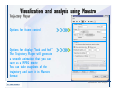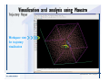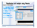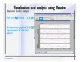
1
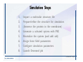
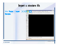
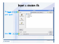
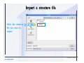
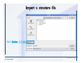
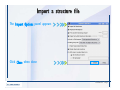
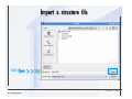
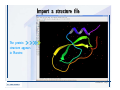
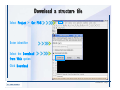
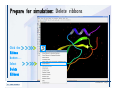
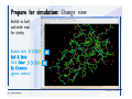
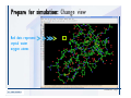
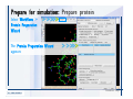
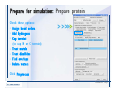
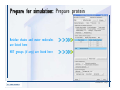
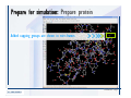
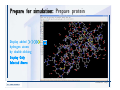
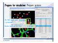
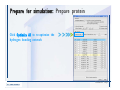
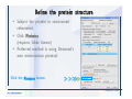
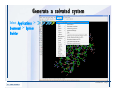
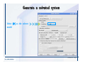
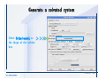
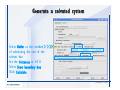
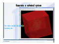
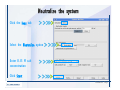
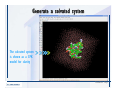
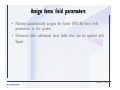
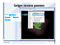
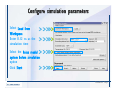
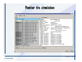
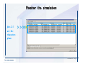
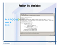
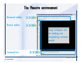
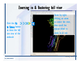
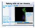
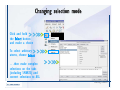
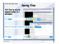
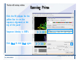
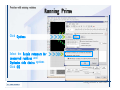
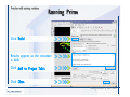
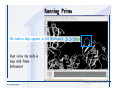
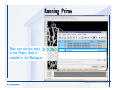
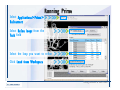
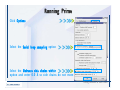
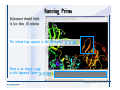
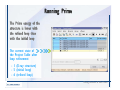
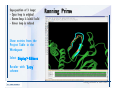
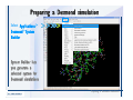
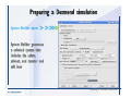
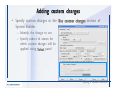
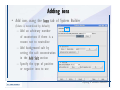
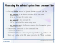
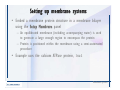
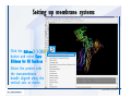
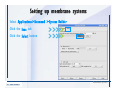
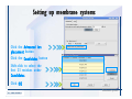
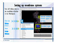
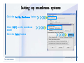
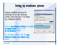
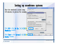
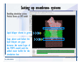
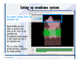
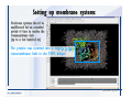
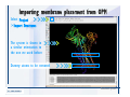
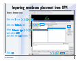
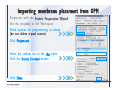
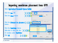
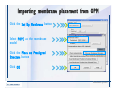
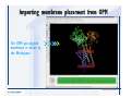
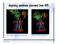
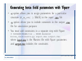
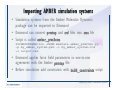
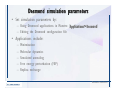
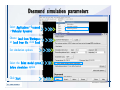
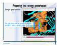
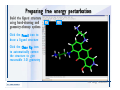
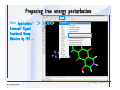
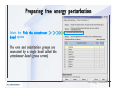
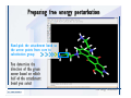
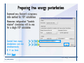
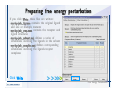
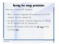
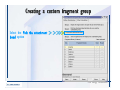
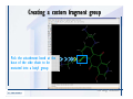
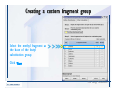
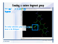
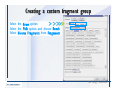
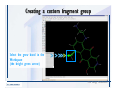
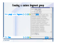
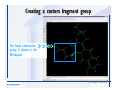
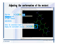
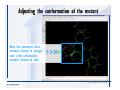
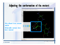
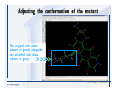
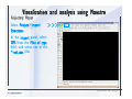
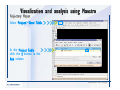
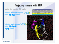
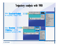
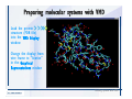
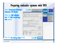
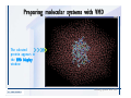
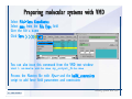
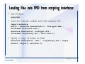
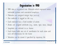
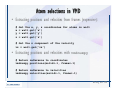
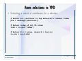
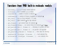
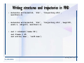
Desmond 2.2 Tutorial Workshop István Kolossváry D. E. Shaw Research www.deshawresearch.com [email protected] Introducing Desmond • Molecular dynamics simulation system • Integrated with Maestro modeling environment, compatible with VMD visualization & analysis tools • Long-scale simulations of small molecules, proteins, nucleic acids, and membrane systems • Study interactions of complex molecular assemblies • Advanced simulation techniques: FEP, simulated annealing, replica exchange, steered dynamics Simulation Steps 1. 2. 3. 4. 5. 6. 7. 8. Import a molecular structure file Prepare/refine the structure for simulation (Immerse the protein in the membrane) Generate a solvated system with PBC Neutralize the system (and add salt) Assign force field parameters Configure simulation parameters Launch Desmond job Simulation Steps Simulation Steps Start Maestro • $SCHRODINGER/maestro • $SCHRODINGER/maestro –SGL (over network) Simulation Steps Start Maestro Maestro main window Simulation Steps Import a structure file Select Project > Import Structures Simulation Steps Import a structure file The Import panel appears Select PDB Simulation Steps Import a structure file Select the structure file you want to import Simulation Steps Import a structure file Click Options Simulation Steps Import a structure file The Import Options panel appears Click Close when done Simulation Steps Import a structure file Click Open Simulation Steps Import a structure file The protein structure appears in Maestro Simulation Steps Download a structure file Select Project > Get PDB Enter identifier Select the Download from Web option Click Download Simulation Steps Prepare for simulation • • • • Delete ribbons Switch to ball-and-stick view for clarity Color carbons green in the structure Prepare the protein for simulation: – – – – Assign bond orders Add hydrogen atoms Remove crystal waters Etc. Simulation Steps Prepare for simulation: Delete ribbons Click the Ribbon button… Select Delete Ribbons Simulation Steps Prepare for simulation: Change view Switch to balland-stick view for clarity Double-click Ball & Stick Click Color By Elements (green carbon) Simulation Steps Prepare for simulation: Change view Red dots represent crystal water oxygen atoms Simulation Steps Prepare for simulation: Prepare protein Select Workflows > Protein Preparation Wizard The Protein Preparation Wizard appears Simulation Steps Prepare for simulation: Prepare protein Check these options: - Assign bond orders - Add hydrogens - Cap termini (to cap N or C termini) - Treat metals - Treat disulfides - Find overlaps - Delete waters Click Preprocess Simulation Steps Prepare for simulation: Prepare protein Residue chains and water molecules are listed here HET groups (if any) are listed here Simulation Steps Prepare for simulation: Prepare protein Added capping groups are shown in wire-frames Simulation Steps Prepare for simulation: Prepare protein Display added hydrogen atoms by double-clicking Display Only Selected Atoms Simulation Steps Prepare for simulation: Prepare protein Selected water molecule Shown with red oxygen atom Hydrogen bond Simulation Steps Prepare for simulation: Prepare protein Optimize the hydrogen bond network by clicking Interactive Optimizer Simulation Steps Prepare for simulation: Prepare protein Click Analyze Network Current protonation states of ASP, GLU and HIS residues are filled in below, as well as OH bond orientations Simulation Steps Prepare for simulation: Prepare protein Select an item to focus the Workspace on a residue Flip through protonation states with the arrow buttons Simulation Steps Prepare for simulation: Prepare protein The OD2 oxygen atom is protonated Residue states can be locked Simulation Steps Prepare for simulation: Prepare protein Click Optimize All to re-optimize the hydrogen bonding network Simulation Steps Refine the protein structure • Subject the protein to constrained refinement • Click Minimize (requires Glide license) • Preferred method is using Desmond’s own minimization protocol Click the Minimize button Simulation Steps Generate a solvated system Select Applications > Desmond > System Builder Simulation Steps Generate a solvated system Select SPC as the solvent model Simulation Steps Generate a solvated system Select Orthorhombic as the shape of the solvent box Simulation Steps Generate a solvated system Select Buffer as the method of calculating the size of the solvent box Set the Distances to 10 Å Select Show boundary box Click Calculate Simulation Steps Generate a solvated system The solute and boundary box Simulation Steps Neutralize the system Click the Ions tab Select the Neutralize option Enter 0.15 M salt concentration Click Start Simulation Steps Generate a solvated system The solvated system is shown as a CPK model for clarity Simulation Steps Assign force field parameters • Maestro automatically assigns the latest OPLS-AA force field parameters to the system • Desmond offers additional force fields that can be applied with Viparr Simulation Steps Configure simulation parameters Select Applications > Desmond > Molecular Dynamics Simulation Steps Configure simulation parameters Select Load from Workspace Enter 0.12 ns as the simulation time Select the Relax model system before simulation option Click Start Simulation Steps Configure job submission options Select Append new entries Enter a name for the simulation and select the Master host Select the subjob Host and run options Click Start Simulation Steps Monitor the simulation Simulation Steps Monitor the simulation Jobs 2-7 are the relaxation phase Simulation Steps Monitor the simulation List of files created by the job Simulation Steps The Maestro environment Horizontal toolbar Vertical toolbar Large workspace area for building and manipulating molecular models Command line Learning Maestro Zooming in & Restoring full view Click the Fit to Screen button to show the full size view of the molecule Zoom by rightclicking an atom to center the view, then scroll the mouse wheel to zoom in or out Learning Maestro Displaying residue and atom information Select View>Sequence Viewer Move the cursor over an atom in the workspace to view its details in the Sequence Viewer Click a residue in the Sequence Viewer to highlight it in yellow in the workspace Learning Maestro Changing selection mode Click and hold the Select button and make a choice To select arbitrary atoms, choose Select …then make complex selections on the tabs (including SMARTS) and convert selections to ASL Learning Maestro Editing a molecular structure Tools for building & editing structures appear when you click the Hammer Hand-draw structures Set chemical elements Increment/decrement bond order or formal charge Adjust the position of atoms Clean up 3D geometry Add common molecular fragments Learning Maestro Projects record every change to molecular structures and results of computational tasks Maestro projects Click the Project button The Project Table opens Each row is an entry Entries are created sequentially Computational tasks can be applied to the state of an entry selected in the table Select the In column to display the entry in the workspace Learning Maestro Useful tools in Maestro • • • • • • • • • • • • Maestro>Save Image saves a screen capture of the workspace Project>Make Snapshot saves the current project state Edit>Clean Up Geometry generates 3D models of hand-drawn structures Edit>Command Script Editor enables powerful scripting Display>Surface generates a variety of molecular surfaces Tools>Sets defines arbitrary sets of atoms for quick rendering Tools>Protein Structure Alignment superposes homologue protein structures Tools>Protein Reports generates useful structural information in a table Applications>Glide is a versatile fast docking tool Applications>LigPrep prepares small molecules for simulation Applications>MacroModel offers molecular mechanics tools Scripts menu for accessing Maestro functionalities from Python scripts Learning Maestro Handling missing residues or side chains • Most protein structures in the PDB database have missing residues, or side chains with missing atoms • Protein Preparation Wizard does not address these issues • Maestro’s Prime tool can automatically build a threedimensional model of a complete amino acid sequence • Prime can be ‘fooled’ into filling in missing residues and side chains in an incomplete protein structure • You need a license for Prime from Schrödinger, LLC Missing Residues & Side Chains Running Prime 1. Download the 1su4 structure to Maestro 2. Delete residues 132-136 from the structure by hand and save it as 1su4 _missing_loop.pdb 3. Import the modified PDB structure into Maestro Ignore the warning message that refers to the missing residues Missing Residues & Side Chains Running Prime The missing loop appears in the structure Colored residues show the position of the missing loop Missing Residues & Side Chains Running Prime Apply Prime to the truncated 1su4 protein structure with the missing loop Simple: Proteins with missing side chains (no missing residues) Complex: Proteins with missing residues Missing Residues & Side Chains Proteins with missing side chains Running Prime Select Applications>Prime> Refinement Select Predict side chains from the Task field Click Start Missing Residues & Side Chains Proteins with missing residues Running Prime Select Applications>Prime> Structure Prediction Click From File… to read in sequence Select the original PDB file Click Open Missing Residues & Side Chains Proteins with missing residues Running Prime Full sequence of residues appears Click Next Missing Residues & Side Chains Proteins with missing residues Running Prime ‘Fool’ Prime by using the truncated structure as a self-template Click Import Select the truncated structure file Click Open Missing Residues & Side Chains Proteins with missing residues Running Prime Click the ID column for the yellow line to see the sequence alignment at the top of the panel Sequence identity is 100% Click Next & click Next again Missing Residues & Side Chains Proteins with missing residues Running Prime Click Options Select the Retain rotamers for conserved residues and Optimize side chains options Click OK Missing Residues & Side Chains Proteins with missing residues Running Prime Click Build Results appear as the structure is built Click Add to Project Table Click Close Missing Residues & Side Chains Running Prime The built-in loop appears in the Workspace Next refine the built-in loop with Prime Refinement Missing Residues & Side Chains Running Prime Make sure the last entry in the Project Table is included in the Workspace Missing Residues & Side Chains Running Prime Select Applications>Prime> Refinement Select Refine loops from the Task field Select the loop you want to refine Click Load from Workspace Missing Residues & Side Chains Running Prime Click Options Select the Serial loop sampling option Select the Unfreeze side chains within option and enter 0.0 Å so side chains do not move Missing Residues & Side Chains Running Prime Click Start Missing Residues & Side Chains Running Prime Refinement should finish in less than 10 minutes The refined loop appears in the Workspace There is no longer a gap in the Sequence Viewer Missing Residues & Side Chains Running Prime The Prime energy of the structure is lower with the refined loop than with the initial loop The current state of the Project Table after loop refinement - 1 (X-ray structure) - 5 (initial loop) - 6 (refined loop) Missing Residues & Side Chains Superposition of 3 loops: - Cyan loop is original - Brown loop is initial build - Green loop is refined Running Prime Show entries from the Project Table in the Workspace Select Display>Ribbons Recolor with ‘Entry’ scheme Missing Residues & Side Chains Preparing a Desmond simulation Select Applications> Desmond>System Builder System Builder lets you generate a solvated system for Desmond simulations Preparing a Desmond Simulation Preparing a Desmond simulation System Builder opens System Builder generates a solvated system that includes the solute, solvent, and counter and salt ions Preparing a Desmond Simulation Selecting solutes and solvents • The current contents of the Workspace constitute the solute (visible or not visible) • Supported solvent models include SPC, TIP3P, TIP4P and TIP4PEW water, and organic solvents DMSO, methanol and octanol • Viparr allows TIP5P and other water models • Custom models are allowed if you provide a pre-equilibrated simulation box of a different solvent molecule Preparing a Desmond Simulation Defining the simulation box • Goal: Reduce the volume of solvent while ensuring that enough solvent surrounds the solute so that the protein does not ‘see’ a periodic image of itself during simulation • Minimize solvent volume by: – Selecting shape that is similar to the protein structure – Applying a reasonable buffer (~10 Å, the typical Coulombic interaction cutoff for long-range electrostatic calculations) – Clicking the Minimize Volume button in System Builder – Applying the truncated octahedron box shape Preparing a Desmond Simulation System Builder output format • Composite model system file with extension .cms • Total solvated system decomposed into 5 sections: – – – – – Protein (solute) Counter ions Positive salt ions Negative salt ions Water molecules • OPLS-AA force field parameters are also written to CMS file Preparing a Desmond Simulation Adding custom charges • Specify custom charges in the Use custom charges section of System Builder – Identify the charge to use – Specify subset of atoms for which custom charges will be applied using Select panel Preparing a Desmond Simulation Adding ions • Add ions using the Ions tab of System Builder (Solute is neutralized by default) – Add an arbitrary number of counterions if there is a reason not to neutralize – Add background salt by setting the salt concentration in the Add Salt section – Specify the type of positive or negative ions to use Preparing a Desmond Simulation Generating the solvated system from command line • Click the Write button in System Builder to save job files – my_setup.mae is the Maestro structure file of the solute Serves as the input for system setup – my_setup.csb is the command file Can be hand-edited for custom setup cases – my_setup-out.cms is the Maestro structure file of simulation system • Execute this command at the command line: $ $SCHRODINGER/run $SCHRODINGER/utilities/system_builder my_setup.csb where my_setup is the file name given to the Write operation Preparing a Desmond Simulation Setting up membrane systems • Embed a membrane protein structure in a membrane bilayer using the Setup Membrane panel – An equilibrated membrane (including accompanying water) is used to generate a large enough region to encompass the protein – Protein is positioned within the membrane using a semi-automated procedure • Example uses the calcium ATPase protein, 1su4 Membrane Systems Setting up membrane systems Select Workflows> Protein Preparation Wizard Enter “1su4” in the PDB field and click Import Check options for preprocessing as shown (do not delete crystal waters) Click Preprocess Membrane Systems Setting up membrane systems Sodium ion is just an artifact of the crystallization process and should be deleted Select the sodium ion in the Het table Click the Delete Selected button Click Close Membrane Systems Setting up membrane systems Click the Ribbon button and select Show Ribbons for All Residues Orient the protein with the transmembrane bundle aligned along the vertical axis as shown Membrane Systems Setting up membrane systems Select Applications>Desmond >System Builder Click the Ions tab Click the Select button Membrane Systems Setting up membrane systems Click the Molecule tab Select Molecule type Select the CA ions The ASL area defines the excluded region Click the Proximity button and set the distance to 5 Å Click OK Membrane Systems Setting up membrane systems Click the Advanced ion placement button Click the Candidates button Shift-click to select the first 23 residues under Candidates Click OK Membrane Systems Setting up membrane systems Turn off ribbon view to see candidate selection in the Workspace Click the Ribbon button… Select Delete Ribbons Selected candidate residues appear as red dots Excluded region Membrane Systems Setting up membrane systems Change the toolbar Select icon to R for residue selection… Select a rectangular area in the Workspace around the transmembrane helices… Membrane Systems Setting up membrane systems Click the Set Up Membrane button Select POPC as the membrane model Click the Select button Membrane Systems Setting up membrane systems Wait until the ASL area is filled Click the Selection button Membrane Systems Setting up membrane systems Switch to ribbon view Workspace shows the initial automatic placement for the protein Click the Ribbon button and select Show Ribbons for All Residues Membrane Systems Setting up membrane systems Adjust the local scope for transformations Check the Adjust membrane position button in the Set Up Membrane window Translate and rotate the membrane model in the Workspace relative to the protein structure Membrane Systems Setting up membrane systems Click the Local transformations icon to switch between local and global scopes as you adjust membrane position Suitable membrane placement Membrane Systems Setting up membrane systems Automate membrane placement for positioning two or more membrane proteins exactly the same in the bilayer (e.g. mutagenesis studies) Click the Save Membrane Position to Selected Entries button in the Set Up Membrane window For subsequent proteins, click the Load Membrane Position from Selected Entry button Membrane Systems Setting up membrane systems Start the membrane system setup 6-8 minutes to process this example Click OK in the Set Up Membrane window Click Start in the System Builder window Membrane Systems Setting up membrane systems Resulting simulation system Protein shown as CPK model Lipid bilayer shown in green Gaps above and below the lipid bilayer are gaps between the water layer of the POPC model and the added water buffer for the simulation box Membrane Systems Setting up membrane systems The protein extends above the simulation box System Builder puts the center of gravity of the solute at the center of the simulation box Non-spherical systems appear to shift toward one side of the simulation box This is a visual artifact, periodic boundary conditions are readily satisfied Membrane Systems Setting up membrane systems Membrane systems should be equilibrated for an extended period of time to resolve the transmembrane hole (up to a few hundred ns) The protein was inserted into a large transmembrane hole in the POPC bilayer Membrane Systems Importing membrane placement from OPM The OPM database at the University of Michigan has high-quality membrane placements Navigate to http://opm.phar.umich.edu/ Enter the protein name and click Search OPM Membrane Systems Importing membrane placement from OPM In the results page, click Download Coordinates Save the file to your computer Membrane Systems Importing membrane placement from OPM Select Project >Import Structures The system is shown in a similar orientation to the one we used before Dummy atoms to be removed Membrane Systems Importing membrane placement from OPM Remove dummy atoms Click the X icon Click the Molecule tab Select Molecule type and select DUM and click the Add button Click OK Membrane Systems Importing membrane placement from OPM Preprocess with the Protein Preparation Wizard Use the structure in the Workspace Check options for preprocessing as shown (do not delete crystal waters) Click Preprocess Select the sodium ion in the Het table Click the Delete Selected button Click Close Membrane Systems Importing membrane placement from OPM Select Applications>Desmond>System Builder Click the Ions tab Click the Select button Click the Advanced ion placement button Click the Candidates button Shift-click to select the first 23 residues under Candidates Click OK Membrane Systems Importing membrane placement from OPM Click the Set Up Membrane button Select POPC as the membrane model Click the Place on Prealigned Structure button Click OK Membrane Systems Importing membrane placement from OPM The OPM pre-aligned membrane is shown in the Workspace Membrane Systems Importing membrane placement from OPM Our manual membrane placement OPM membrane placement Membrane Systems Importing membrane placement from OPM Click Start in the System Builder to generate the membrane Our full membrane simulation system OPM full membrane simulation system Membrane Systems Importing membrane placement from OPM Our transmembrane hole OPM transmembrane hole Membrane Systems Generating force field parameters with Viparr • • • • • • • • • Assign alternative force field parameters with Viparr Viparr is a Python script that reads .cms (or .mae) files Refers to a template database to assign force field parameters Matches residues to templates using atomic numbers & bond structure Built-in force fields include latest versions of Amber, CHARMM, and OPLS-AA for fixed charge model and pff polarizable force field Wipes out existing ffio_ff{ } structure in the .cms input file Does not alter atom or residue ordering when creating the output file Recommended: perform post-processing on .cms with Viparr Invoke from command line: $SCHRODINGER/run –FROM desmond viparr.py --help Force Fields with Viparr Generating force field parameters with Viparr • Can specify multiple force fields • Example: $ viparr.py –f charmm27 –f tip4p 1su4_desmond.cms 1su4_desmond_out.cms • Combine components of two or more force fields • All matching force fields are applied • Conflicting parameters: first force field in command line invocation takes precedence • Viparr aborts if a bond exists between two residues that are not matched by the same force field, or if force fields have inconsistent van der Waals combining rules Force Fields with Viparr Generating force field parameters with Viparr • Viparr generates error or warning messages when: – A residue matches more than one template in a force field – A residue name is matched to a force field template with a different name – There are unmatched residues – A residue is matched by more than one of the selected force fields Force Fields with Viparr Generating force field parameters with Viparr • -c option allows you to assign parameters for a particular structure (f_m_ct{ } block) in the input .cms file • -n option allows you to include comments in the output .cms file for annotation purposes • You must add constraints in a separate step with Viparr: $ $SCHRODINGER/run – FROM desmond build_constraints.py input.cms output.cms where input.cms is the Maestro file with Viparr parameters and output.cms includes the constraints Force Fields with Viparr Importing AMBER simulation systems • Simulation systems from the Amber Molecular Dynamics package can be imported to Desmond • Desmond can convert prmtop and crd files into cms file • Script is called amber_prm2cms $SCHRODINGER/run –FROM mmshare amber_prm2cms.py –p my_amber_system.prm –c my_amber_system.crd -o output.cms • Desmond applies force field parameters in one-to-one agreement with the Amber prmtop file • Before simulation add constraints with build_constraints script Importing Amber Simulation Systems Desmond simulation parameters • Set simulation parameters by: – Using Desmond applications in Maestro (Applications>Desmond) – Editing the Desmond configuration file • Applications include: – – – – – Minimization Molecular dynamics Simulated annealing Free energy perturbation (FEP) Replica exchange Desmond Simulation Desmond simulation parameters Select Applications>Desmond >Molecular Dynamics Choose Load from Workspace or Load from file, click Load Set simulation options Select the Relax model system before simulation option Click Start Desmond Simulation Desmond simulation parameters Click Advanced Options • • • • • • Integration—Set multiple time step parameters and constraints Ensemble—Set thermostat and barostat parameters Interaction—Set parameters for computing non-bonded interactions Restraint—Subject multiple sets of atoms to harmonic restraint with a tunable force constant Output—Control output file names and specify how often files are updated during simulation Misc—Set miscellaneous parameters including the definition of atom groups or the construction of trajectory files Desmond Simulation Running Desmond simulations • Run Desmond simulations by: – Clicking Start in the Molecular Dynamics window – Entering commands at the command line • Structure relaxation prepares the system for production-quality MD simulation • Maestro’s relaxation protocol includes: – 2 stages of minimization (restrained and unrestrained) – 4 stages of short MD runs with gradually diminishing restraints and increasing temperature Running Simulations Running Desmond simulations Click Start Running Simulations Running Desmond simulations Select Append new entries to add results to the current project Enter a name for the job Select the host where the master job should run; usually localhost Set job submission parameters Click Start Running Simulations Running Desmond simulations • Run simulations from the command line: $SCHRODINGER/desmond -HOST <hostname> -exec <desmond_task> -P <cpu> -c <jobname>.cfg –in <jobname>.cms • where: can be minimize (simple minimization), mdsim (MD simulation), vrun (trajectory analysis) jobname is the name of the job hostname is the name of the compute host or queue on a cluster cpu specifies the number of CPUs you want each Desmond simulation subjob to use (either 1 for quick tests or a power of 2) – desmond_task – – – Running Simulations Running Desmond simulations • Advanced issues to consider: – The Desmond driver tries automatically to optimize configuration parameters; turn this off using the -noopt argument – Automatically generate Desmond configuration settings for efficient force computations with the forceconfig script: $SCHRODINGER/run -FROM desmond forceconfig.py <input.cms> – While a Desmond job is running, all files for the job are continuously updated in a temporary directory: tmpdir/username/jobname where tmpdir is specified in $SCHRODINGER/schrodinger.hosts Use -LOCAL option to keep job files in the working directory Running Simulations Running Desmond simulations • Run multiple jobs from the command line – May be necessary for system relaxation and FEP simulations – Multiple jobs are handled by the MultiSim facility – Reads a .msj command script file and runs simulations defined within it • $SCHRODINGER/utilities/multisim -JOBNAME <jobname> -maxjob <maxjob> -cpu <cpu> -HOST localhost -host <hostname> -i <jobname>.cms -m <jobname>.msj -o <jobname>-out.cms is the maximum # of simultaneous subjobs (0=no limit) cpu is the # of CPUs per subjob (8 CPUs can be “2 2 2”) hostname is the host or queue where simulation jobs will run – maxjob – – Running Simulations Preparing free energy perturbation • Desmond can run free energy perturbation (FEP) calculations: – Ligand and amino acid residue mutation – Annihilation (absolute free energy calculation) – Single-atom mutation in a ring structure • Visually specify fixed and variable parts of a molecule for defining the mutation • Store the atom correspondence map in the .mae file (dual topology) Free Energy Perturbation Preparing free energy perturbation Example ligand mutation This side chain will be mutated to replace the NH3+ with a methyl group Free Energy Perturbation Preparing free energy perturbation Build the ligand structure using hand-drawing and geometry-cleanup options Click the Pencil icon to draw a ligand structure Click the Clean Up icon to automatically correct the structure to give reasonable 3-D geometry Free Energy Perturbation Preparing free energy perturbation Select Applications> Desmond>Ligand Functional Group Mutation by FEP… Free Energy Perturbation Preparing free energy perturbation Select the Pick the attachment bond option The core and substitution groups are connected by a single bond called the attachment bond (green arrow) Free Energy Perturbation Preparing free energy perturbation Hand-pick the attachment bond so the arrow points from core to substitution group You determine the direction of the green arrow based on which half of the attachment bond you select Free Energy Perturbation Preparing free energy perturbation Select the fragment that will replace the substitution group For multiple fragments, FEP creates different systems for each mutant and computes binding free energy difference between reference ligand and each selected mutant, with respect to the receptor Click Start Free Energy Perturbation Preparing free energy perturbation Desmond uses Bennett’s acceptance ratio method for FEP calculations Numerous independent “Lambda window” simulations will be run for a single FEP calculation Control how many simulations can run simultaneously 0 = no limit Click Start Free Energy Perturbation Preparing free energy perturbation If you click Write, these files are written: -my-fep-job_lig.mae contains the original ligand and one or multiple mutants -my-fep-job_cmp.mae contains the receptor and ligand structures -my-fep-job_solvent.msj defines a series of simulations involving the ligands in the solvent -my-fep-job_complex.msj defines corresponding simulations involving the ligand-receptor complexes Click Write Free Energy Perturbation Running free energy perturbation Three ways of running FEP simulations: • Write a Desmond configuration file yourself and run the FEP simulation from the command line • Use Maestro to generate a Desmond configuration file and run the FEP simulation from the command line • Run the FEP simulation directly from the FEP Setup window by clicking Start Free Energy Perturbation Generating a Desmond FEP configuration file Select Applications> Desmond>FEP Free Energy Perturbation Generating a Desmond FEP configuration file Select the windows that should be included in the simulation Click Write Free Energy Perturbation Running FEP simulation from the command line • Run FEP simulations using a .msj command script file $SCHRODINGER/utilities/multisim -JOBNAME <jobname> -maxjob <maxjob> -cpu <cpu> -HOST localhost -host <hostname> -i <jobname>.mae -m <jobname>.msj -o <jobname>-out.mae is the name of the job maxjob is the maximum number of subjobs that can be submitted simultaneously (0 means no limit) cpu is the number of CPUs per subjob (8 CPUs can be shown as “2 2 2”) -HOST localhost means the master job runs on your local workstation -host <hostname> is the host or queue where the simulation jobs will run – jobname – – – – • To apply non-default FEP parameters or change the number of Lambda windows, add the -cfg <config_file> option and provide the name of the file generated by the FEP window Free Energy Perturbation Computing free energy difference • Run the bennett.py script from the command line to process the “energy” file output of the different Lambda runs and compute the free energy $SCHRODINGER/run -FROM desmond bennett.py [--help] • or from Maestro, import the –out.cms file and the delta G free energy difference can be displayed in the Project Table • The delta-delta G relative binding free energy difference is equal to delta G “complex” – delta G “solvent” Free Energy Perturbation Creating a custom fragment group • Edit any pre-defined substitution group manually with the Build/Edit tools in Maestro • Mutations of more than a few atoms are subject to large uncertainties in the free energy differences computed between different Lambda windows • Decompose large mutations into several smaller mutations and run multiple MultiSim FEP simulations Free Energy Perturbation Creating a custom fragment group Select the Pick the attachment bond option Free Energy Perturbation Creating a custom fragment group Pick the attachment bond at the base of the side chain to be mutated into a butyl group Free Energy Perturbation Creating a custom fragment group Select the methyl fragment as the base of the butyl substitution group Click View Free Energy Perturbation Creating a custom fragment group Select Edit> Fragments The methyl substitution group is shown in the Workspace Free Energy Perturbation Creating a custom fragment group Select the Grow option Select the Pick option and choose Bonds Select Diverse Fragments from Fragments Free Energy Perturbation Creating a custom fragment group Select the grow bond in the Workspace (the bright green arrow) Free Energy Perturbation Creating a custom fragment group Select propyl under Fragments Click Close Free Energy Perturbation Creating a custom fragment group The butyl substitution group is shown in the Workspace Free Energy Perturbation Adjusting the conformation of the mutant • Initial conformation of the mutant must be as close as possible to the original side chain for FEP simulations • Manual adjustments to the conformation of small molecules can be readily done in Maestro • Use Maestro’s Adjustment tool to make manual adjustments Free Energy Perturbation Adjusting the conformation of the mutant Click the Adjustment icon to make manual adjustments Select the attachment bond to display the non-bonded contacts Free Energy Perturbation Adjusting the conformation of the mutant Note the numerous close contacts (shown in orange) and a few unfavorable contacts (shown in red) Free Energy Perturbation Adjusting the conformation of the mutant • Adjust the torsion angle manually using the Adjustment Tool’s “Quick Torsion” option: – Hold down the left mouse button and move the mouse horizontally – or Rotate the mouse wheel • Relax the unfavorable contacts iteratively with rotations about different bonds in the side chain Free Energy Perturbation Adjusting the conformation of the mutant Only allowed close contacts remain Unfavorable contacts have been removed Free Energy Perturbation Adjusting the conformation of the mutant The original side chain (shown in green) alongside the modified side chain (shown in grey) Free Energy Perturbation Other types of mutations • Protein residue mutation – Compute the difference in free energy for a ligand bound to a protein versus the same ligand bound to a mutated form of the same receptor with amino acid residue mutations applied to the protein – Compute the difference in free energy for a protein versus a mutated protein, without a ligand • Ring atom mutation – replace one atom with another in a ring structure • Absolute or total free energy calculation – Compute absolute solvation free energy (and absolute binding free energy) by annihilating a whole solute or ligand molecule Free Energy Perturbation Visualization and analysis using Maestro • Maestro offers basic visualization and analysis tools • Trajectory Player – Similar to the ePlayer in the Project Table – Designed to animate Desmond trajectories • Simulation Quality Analysis window – Performs basic quality analysis – Shows statistical properties of basic thermodynamic quantities based on block averages • Schrödinger add-on scripts – Simulation Event Analysis – Trajectory cluster analysis Visualization and Analysis Visualization and analysis using Maestro Trajectory Player Select Project>Import Structures In the Import panel, select CMS from the Files of type field, and select one of the *-out.cms files Visualization and Analysis Visualization and analysis using Maestro Trajectory Player Select Project>Show Table In the Project Table click the T button in the Aux column Visualization and Analysis Visualization and analysis using Maestro Trajectory Player Options for frame control Options for display “look and feel” The Trajectory Player will generate a smooth animation that you can save as a MPEG movie You can take snapshots of the trajectory and save it in Maestro format Visualization and Analysis Visualization and analysis using Maestro Trajectory Player Workspace view for trajectory visualization Visualization and Analysis Visualization and analysis using Maestro Simulation Quality Analysis Select Applications>Desmond >Simulation Quality Analysis Click Browse and select the energy file (desmond_job.ene) Click the Analyze button Results of analysis appear Visualization and Analysis Visualization and analysis using Maestro Simulation Quality Analysis Click the Plot button An interactive graphical representation of the data appears Visualization and Analysis Trajectory analysis with VMD • VMD is a widely used molecular visualization platform providing a plethora of tools for trajectory analysis: – – – – Strong support for atom selections Ability to efficiently animate trajectories with thousands of snapshots Support for Tcl and Python scripting languages Built-in capability to write Maestro files (useful to prepare simulation system in VMD) and read Desmond trajectory files (useful for analyzing Desmond trajectories) These features are available in the new VMD 1.8.7 Visualization and Analysis Trajectory analysis with VMD • VMD Python interface – Access from console (terminal from which you launched VMD) vmd>gopython – Access from Idle window that runs inside VMD (preferred) vmd>gopython –command “import vmdidle; vmidle.start()” – Copy command into .vmdrc file – Some modules are provided by the Python interpreter when you launch Python, others are loaded at runtime – VMD provides built-in modules for loading data into VMD, querying and modifying VMD state: molecule module, atomsel module, vmdnumpy module Visualization and Analysis Trajectory analysis with VMD • Loading and viewing trajectories – Structure files (.mae or .cms) • • • • • Created by Maestro or Desmond Contain topology, mass, charge, and possibly force field information Single molecular system including solvent or ions Single snapshot of positions of atoms and virtual sites Select the Maestro mae file type to select these files – Trajectory files (.dtr) • • • • Created by Desmond Directory that contains metadata files and frame files holding snapshots .dtr files load positions, .dtrv files load positions and velocities Select the clickme.dtr file Visualization and Analysis Trajectory analysis with VMD • Loading files from the command line – vmd –mae structure.cms –dtr trajectory_subdir/clickme.dtr – This command: • • • • Creates a new molecule Initializes its structure from the cms file Creates an initial set of coordinates from the cms file Appends all snapshots from the dtr file to the molecule – Load multiple structure and trajectory files with -m and -f • -m causes a new molecule to be created for each subsequent file • -f causes subsequent files to be loaded into the same molecule • vmd -m -mae mol1.mae mol2.mae -f mol3.mae -dtr trajectory_subdir/clickme.dtr Visualization and Analysis Trajectory analysis with VMD Loading files from the VMD window Select File>New Molecule Click Browse and select the structure file Click Load Click Browse again In the Choose a molecule file window select the clickme.dtr “trajectory file” you want to use Click Load again Visualization and Analysis Trajectory analysis with VMD Loading files from the VMD window Molecular information appears in the VMD Main window Trajectory movie appears in the VMD OpenGL Display window Visualization and Analysis Trajectory analysis with VMD Select Extensions>Analysis for trajectory analysis tools Select Extensions >Modeling to set up simulation systems in VMD Visualization and Analysis Preparing molecular systems with VMD • Load a molecule into VMD • Use VMD modeling tools to generate the simulation system (the main building tool is Automatic PSF Builder) • Save the system in a Maestro file (File>Save Coordinates) • Add force field parameters and constraints with Viparr and the build_constraints script Building Systems with VMD Preparing molecular systems with VMD Load the protein structure (PDB file) into the VMD Display window Change the display from wire frame to “licorice” in the Graphical Representations window Building Systems with VMD Preparing molecular systems with VMD Select Extensions>Modeling> Automatic PSF Builder Select the Add solvation box and Add neutralizing ions options Click the I’m feeling lucky button Building Systems with VMD Preparing molecular systems with VMD The solvated protein appears in the VMD Display window Building Systems with VMD Preparing molecular systems with VMD Select File>Save Coordinates Select mae from the File Type field Give the file a name Click Save You can also issue this command from the VMD text window: vmd > animate write mae my_output_file.mae Process the Maestro file with Viparr and the build_constraints script to add force field parameters and constraints Building Systems with VMD Loading files into VMD from scripting interfaces • Start Python: gopython • Load the molecule module and read structure file: import molecule molid = molecule.read(molid=-1, filetype=‘mae’, filename=‘structure.cms’) molecule.read(molid, filetype=‘dtr’, filename=‘trajectory.dtr’, wait-for=-1) • Specify a range of frames to load: molecule.read(molid, ‘dtr’, ‘trajectory.dtr’, beg=5, end=55, skip=10, waitfor=-1) Working with VMD Organization in VMD • VMD data is organized into Molecules which represent entire molecular systems and associated snapshots • Molecules are assigned integer keys (molid) • One molecule is tagged as the top • Each molecule has a fixed number of atoms • Atoms are assigned attributes (e.g., name, type, mass, charge) • Snapshots are referred to as frames • Each frame holds one set of coordinates for each atom and unit cell dimensions for the frame • Velocities can be stored if specified by trajectory file Working with VMD Atom selections in VMD • Consist of all the atoms in a particular molecule and frame that satisfy a predicate or set of conditions • Could be different for different frames • Scripting interface uses atom selection to specify a predicate for an atom selection object • Atom selection objects created in VMD Python with atomsel module Import the atomsel type from atomsel import atomsel Create a selection of atoms in the top molecule for the current frame all = atomsel() Working with VMD Atom selections in VMD # Select atoms named ‘CA’ in top molecule in current frame ca = atomsel(selection=‘name CA’) # Select protein atoms in frame 10 of top molecule pro10 = atomsel(‘protein’, frame=10) # Select waters near the protein from molecules 0 and 1 wat0 = atomsel(‘water and same residue as (within 5 of protein)’, molid=0) wat1 = atomsel(‘water and same residue as (within 5 of protein)’, molid=1) Working with VMD Atom selections in VMD • The – – – atomsel type takes three arguments: Selection – Selection predicate Molid – Molecule associated with the selection Frame – Index of the snapshot referenced by the selection • Setting the frame attribute n1 = len(wat0) f = wat0.frame wat0.frame = 20 n2 = len(wat0) wat0.update() n3 = len(wat0) # # # # # # number of atoms in the selection returns -1 makes wat0 reference frame 20 will be equal to n1 recompute selection on frame 20 might be different from n1 • Changing the frame does not cause the selection to be recomputed • Only the update() method changes the atoms referenced • Changing the frame does change the result of calculations that depend on the coordinates (e.g. center() or rmsd()) Working with VMD Atom selections in VMD • Extracting data about a molecule for the selected atoms: # Get the number of alpha carbons num_ca = len(ca) # Get the residue name of each alpha carbon resnames = ca.get(‘resname’) # Set the ‘type’ attribute of all atoms to ‘X’ all.set(‘type’, ‘X’) # Compute the center of mass of atoms in frame 10 mass = pro10.get(‘mass’) com = pro10.center(mass) # Align pro10 to atoms in frame 0, compute RMSD pro0 = atomsel(‘protein’, frame=0) m = pro10.fit(pro0, weight=mass) pro10.move(m) rms = pro10.fit(pro0) Working with VMD Atom selections in VMD • Extracting positions and velocities from frames (expensive): # x y z Get the x, y, z coordinates for atoms in wat1 = wat1.get(‘x’) = wat1.get(‘y’) = wat1.get(‘z’) # Get the z component of the velocity vz = wat1.get(‘vz’) • Extracting positions and velocities with vmdnumpy # Return reference to coordinates vmdnumpy.positions(molid=-1, frame=-1) # Return reference to velocities vmdnumpy.velocities(molid=-1, frame=-1) Working with VMD Atom selections in VMD • Extracting a subset of coordinates for a selection # Return all positions in top molecule’s current frame pos = vmdnumpy.positions() # Return index of all CA atoms inds = ca.get(‘index’) # Return M x 3 array, where M = len(ca) ca_pos = pos[inds] Working with VMD Functions from VMD built-in molecule module – molid of newly created molecule listall() – list of available molid values numatoms(m) – number of atoms in molecule m numframes(m) – number of frames (snapshots) in molecule m get_top() – molid of top molecule; -1 if none set_top() – make molecule m the top molecule get_frame() – get current frame for molecule m set_frame(m,frame) – set current frame for molecule m to frame get_periodic(m=-1, frame=-1) – dictionary of periodic cell data set_periodic(m=-1, frame=-1) – set periodic cell keywords get_physical_time(m=-1, frame=-1) – time value for timestep read(molid, filetype, filename, …) – load molecule files write(molid, filetype, filename, …) – save molecule files • new(name) • • • • • • • • • • • • Working with VMD Writing structures and trajectories in VMD • molecule.write(molid, ‘dtr’, ‘trajectory.dtr’, waitfor=-1) • molecule.write(molid, ‘dtr’, ‘trajectory.dtr’, beg=100, end=-1, skip=10, waitfor=-1) • sel = atomsel(‘name CA’) sel.frame = 45 sel.write(‘mae’, ‘ca45.mae’) Working with VMD Analyzing whole trajectories in VMD • Script runs through frames in a molecule, aligns frames to the first frame, and computes the aligned RMSD for each frame and the averaged position of the alpha carbons from atomsel import atomsel import molecule, vmdnumpy import numpy avg = None # holds averaged coordinates all = atomsel() # all atoms in current frame ref = atomsel(‘name CA’, frame = 0) # reference frame 0 sel = atomsel(‘name CA’) # alpha carbons, current frame inds = sel.get(‘index’) # indexes of alpha carbons mass = sel.get(‘mass’) # masses of alpha carbons rms = [0.] # holds RMSD, reference frame Working with VMD Analyzing whole trajectories in VMD def processFrame(): global avg # Align current frame with reference frame all.move( sel.fit(ref, mass) ) # Append new RMSD value rms.append( sel.rmsd(ref, mass) ) # Get positions of CA atoms pos = vmdnumpy.positions() ca_pos = pos[inds] # Accumulate positions into average if avg is None: avg = ca_pos[:] # Make a copy of ca_pos else: avg += ca_pos # Add this frame’s contribution # Loop over frames n = molecule.numframes(molecule.get_top() for i in range(1,n ): molecule.set_frame(molecule.get_top(), i) processFrame() # Scale the average avg /= n Working with VMD Documentation Resources • • • • • • • Desmond Tutorial Desmond User’s Guide Desmond user community website: http://groups.google.com/group/desmond-md-users/ Schrödinger’s Desmond documentation: – Quick Start Guide: $SCHRODINGER/docs/desmond/quick_start/des22_quick_start.pdf – Desmond User Manual: $SCHRODINGER/docs/desmond/user_manual/des22_user_manual.pdf Maestro documentation: – Maestro Overview: $SCHRODINGER/docs/maestro/overview/mae90_overview.pdf – Maestro Command Reference: $SCHRODINGER/docs/maestro/ref_manual/mae90_command_reference.pdf – Maestro Tutorial: $SCHRODINGER/docs/maestro/tutorial/mae90_tutorial.pdf – Maestro User Manual: $SCHRODINGER/docs/maestro/user_manual/mae90_user_manual.pdf ASL documentation: $SCHRODINGER/docs/maestro/help/mae90_help/misc/asl.html Prime documentation – Prime Quick Start: $SCHRODINGER/docs/prime/quick_start/pri21_quick_start.pdf – Prime User Manual: $SCHRODINGER/docs/prime/user_manual/pri21_user_manual.pdf Documentation Resources