Download Analysis and Status

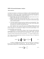
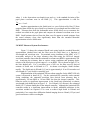
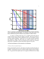
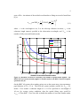
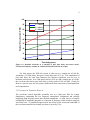
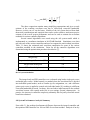
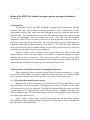
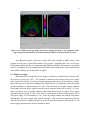
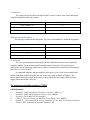
MMTO Technical Memorandum #12-1
MMT AO Performance:
Analysis and Status
K. Powell
April 2012
MMT AO System Performance Analysis
1.0 Introduction
A systems level analysis of wavefront error contribution is useful for understanding what
areas of the AO system can be improved to provide the greatest performance increases
and, therefore, maximize image quality. For the MMT-AO system, major contributors to
wavefront error can be divided into three distinct components:
1) Spatial fitting errors due to the limited number of spatial modes that can be
applied to the deformable mirror at any instant in time.
2) Temporal errors due solely to the pure time delay of the wavefront sensor (WFS).
This delay manifests itself as an error in the reconstructed wavefront surface input
to the wavefront controller.
3) Wavefront controller temporal errors due to limited correction bandwidth. These
errors affect both the magnitude and phase of the wavefront surface input signal,
attenuating some components and amplifying others.
Other significant sources of wavefront error exist including isoplanatic effects and
sensor noise. However, since reducing wavefront error from these components would
involve integration of new hardware or changes to the current system design, it was
deemed beyond the scope of this study.
The Strehl ratio is often used as a figure of merit for image quality when the
imaging application is at or near the diffraction limit, such as adaptive optics. The Strehl
ratio is defined as the ratio of the measured on-axis peak intensity I p from a point source
compared with the maximum theoretical peak intensity I T for a perfect imaging system.
For a circular aperture and pupil plane wavefront error function of    ,  expressed in
polar coordinates, we have
Ip
1
Strehl   2
IT 
1 2
 2 i

0 0 exp      ,   d  d
2
(1.1)
A number of simplified approximations exist for the Strehl ratio as a function of
the root mean squared (RMS) wavefront error. The most commonly used of these
approximation is known as the extended Marechal approximation and is given by
2
 2
 
Strehl  exp   nm  
 
 
(1.2)
2
where  is the observation wavelength in nm and  nm is the standard deviation of the
pupil plane wavefront error in nm RMS [1]. This approximation is valid for
2
 nm  1 rad .

Another approximation to the Strehl ratio is a curve-fit derived by Hart [2] from
empirical data which also gives Strehl as a function of wavelength and wavefront error
RMS. Telemetry data from the deformable mirror (DM) allows us to reconstruct the
residual wavefront in the pupil plane and compute an estimated wavefront error in nm
RMS. Strehl estimates derived from the Hart curve-fit appear to match estimates from
the actual telemetry slope data significantly better than the extended Marechal
approximation at lower Strehl ratios.
2.0 MMT Measured System Performance
Figure 2.1 shows the estimated Strehl ratio using both the extended Marechal
approximation (dashed lines) and the Hart curve-fit (solid lines) as a function of
wavelength and wavefront error. For nominal seeing conditions at the MMT of 0.77
arcseconds, analysis of the slope telemetry data when using the NGS-AO integral
wavefront controller shows that the estimated wavefront error RMS is approximately 450
nm. Analyzing the telemetry data at various seeing conditions and pointing angles
relative to the wind gives a typical range of 75 nm RMS. This is shown in figure 2.1 as
the blue shaded area. For a wavefront error of 450 nm, the Hart curve-fit derived
estimate of Strehl ratio in M-band is 0.75. At shorter wavelengths, Strehl declines
rapidly. The Strehl ratio in H-band (1.65 µm) is approximately 0.18 at 450 nm and at red
wavelengths (0.7 µm) Strehl is essentially zero.
Implementation of the optimized PID wavefront controller for the MMT NGS-AO
system is discussed in detail in [3]. For the optimized PID controller under nominal
seeing conditions, the estimated wavefront error derived from telemetry data is
approximately 340 nm RMS or 110 nm RMS less than the integral controller. This
behavior results in significant improvement in the Strehl ratio particularly at shorter
wavelengths (red shaded area in figure 2.1). For H-band (1.65 microns), the estimated
Strehl is 0.33, almost double that of the integral controller. Although the optimized PID
controller results in a significant improvement in Strehl, additional reductions in the
wavefront residual are required if we want to achieve high Strehl in H-band and
particularly if we want to have diffraction limited imaging down to J-band (1.25 µm) and
good correction at visible wavelengths.
3
1
0.8
0.6
Strehl
PID
Controller
Integral
Controller
0.4
0.2
0
0
100
200
300
400
500
600
Wavefront error (nm RMS)
Figure 2.1: Strehl ratio as a function of wavefront error RMS and wavelength. Dashed lines
are the extended Marechal approximation. The solid lines are Hart curve-fit data. Red
lines are M-band (5 µm), green are H-band (1.65 µm), and blue are visible at 700 nm.
To obtain a reasonable Strehl ratio of 0.5 in H-band would require that the
residual wavefront error be reduced to roughly 250 nm RMS. This level of correction is
possible to achieve through software modifications only by the development of better
wavefront controller algorithms. Strehl ratios of 0.5 in J-band would be significantly
more difficult to obtain and would require the residual wavefront error to be
approximately 180 nm RMS. This level of reduction in the wavefront error would most
likely require a combination of software and hardware upgrades to the system.
3.0 Theoretical Estimates of Wavefront Error Contributions
3.1 SPATIAL FITTING ERROR ESTIMATE
Because the deformable mirror has a finite limit to the number of spatial modes that can
be applied, the mirror will never exactly match the spatial structure of the atmospheric
turbulence. This limitation results in a wavefront residual component known as fitting
error. In general, the more spatial modes we can apply to the DM, the less the fitting
4
error will be. An estimate of the residual wavefront due to fitting error can be found from
[4] as
12
53

 
 32D
 fitting  nm RMS   0.2944 N Zern   
2 
 r0  

(3.1)
where  is the wavelength in nm, D is the telescope diameter in meters, r0 is the
coherence length (meters) specified at the observation wavelength, and N Zern is the
number of fully corrected Zernike modes.
Residual wavefront (nm RMS)
500
r0 = 0.1
r0 = 0.15
r0 = 0.2
400
300
200
100
0
0
20
40
60
80
100
120
Number of corrected Zernike modes
Figure 3.1: Residual wavefront as a function of the number of spatial modes applied. The
MMT NGS-AO system currently applies 54 Zernike modes to the DM. Coherence length is
specified at 0.5 µm.
On the MMT AO system, the secondary mirror acts as the system stop, given an entrance
pupil diameter of D = 6.3 m. The NGS-AO system currently corrects for N Zern  54
modes. If we assume a coherence length of r0  0.15 m specified at a wavelength of
0.5 m for average seeing conditions, then the spatial fitting error would be
 fitting  175nm RMS . If we were able to double the number of corrected Zernike modes
5
applied to the DM, N Zern  108 , the spatial fitting error would then be
 fitting  130nm RMS , for a total difference of 45 nm RMS. Figure 3.1 shows the spatial
fitting error as a function of coherence length and the number of fully corrected Zernike
modes for the MMT AO system.
3.2 PURE TIME DELAY ERROR DUE TO WFS
Wavefront errors due to pure time delay effects of the WFS are fundamentally different
than errors associated with the temporal response of the controller, which will be
addressed in the following section. Pure time delays are important particularly in the
case of high altitude wind speeds associated with the jet stream. Jet stream winds can
reach speeds in excess of 80 m/s and typically occur at altitudes of 10-15 km. Time
delays can also be important for faint targets when the sample rate must be lowered to
obtain a reasonable signal to noise ratio on the wavefront sensor (WFS).
For a single turbulent atmospheric layer, we can approximate the Greenwood
frequency as a function of wind speed v and coherence length r0    , which in turn is a
function of observation wavelength.
f g  0.427
v
r0   
(3.2)
Fried [5] and Karr [6] independently investigated the effects of pure time delay on the
wavefront error. Assuming Kolmogorov turbulence is measured and a correction is
applied after a time delay of  s , then the wavefront error due to the pure time delay can
be written as [1]
 TD  nm RMS  
53 12
 

28.4

f

s g 



2
(3.3)
Figure 3.2 shows the residual wavefront as a function of time delay and wind
speed. This particular case assumes an observation wavelength of   1.65m (H-band)
and a coherence length of 0.6m, also specified at H-band. Delay time due to the WFS
camera is known to be approximately 1.5 frames. The typical sample rate for the NGSAO system for bright targets is 550 Hz, which gives a total delay time of 2.7 msec. At
moderate high altitude wind speeds of 20 m/s, the wavefront error due to the 1.5 frame
delay time is less than 30 nm RMS. However, for large wind speeds the contribution of
wavefront error can become significant. At a wind speed velocity of 60 m/s, the
wavefront error is approximately 70 nm RMS.
6
100
Residual Wavefront (nm RMS)
90
80
V = 20 m/s
V = 40 m/s
V = 60 m/s
70
60
50
40
30
20
2
2.5
3
3.5
4
Time delay (msec)
Figure 3.2: Residual wavefront as a function of pure time delay and wind velocity.
Greenwood frequency assumes an r0=0.6m in H-band (r0=0.15m at 0.5 µm).
For faint targets, the NGS-AO system is often run at a sample rate of 100 Hz.
Assuming a 1.5 frame delay, this gives a total delay time of 15 ms. The contribution of
pure time delay for such large latencies also becomes significant even for low to
moderate wind speeds. At a wind speed velocity of 20 m/s and a sample rate of 100 Hz,
the wavefront error due to pure time delay is on the order of 100 nm RMS. Clearly for
these two special cases, the AO system could benefit from some form of wind prediction
and compensation.
3.3 CONTROLLER TEMPORAL EFFECTS
The wavefront control algorithm essentially acts as a high pass filter for system
disturbances, attenuating the low frequency atmospheric components and possibly
amplifying high frequency noise and vibration components. As such, there is a complex
relationship of magnitude and phase as a function of frequency which results in temporal
wavefront error. A simplified expression for the effects of the correction bandwidth of
the wavefront controller on residual wavefront is given by [2] as
7

 Control  nm RMS  
2
12
  f g 5 3 

 
 f 3dB  
(3.4)
The above expression contains many simplifying assumptions and gives a crude
estimate of the resulting wavefront error due to closed-loop correction bandwidth.
However, in this case we can do better. Models of the AO system derived from both
theoretical considerations and empirical data can be used to obtain a much more precise
estimate of the overall system performance and can be used to estimate the wavefront
residuals for various controller algorithms.
Several control algorithms were tested using the AO system model which is
implemented as a nonlinear simulation in MATLAB/Simulink. Simulations were then
run with each of the various controllers and used to compute the total residual wavefront.
Table 3.1 shows the estimated total wavefront contribution for some of the various
controllers modeled in the simulation. Gains for all the controller algorithms were
determined using the optimization procedure described in [7].
Control algorithm
Total residual wavefront (nm RMS)
Integral only
447
Proportional, Integral, Derivative (PID)
347
Integral with modal gains
438
PID with modal gains
329
Table 3.1: Evaluation of residual wavefront error for different controller topologies using
the AO system simulation.
The integral only and PID controllers were evaluated using both a single gain vector
and modal gain vectors. Modal control is a method where the wavefront error is divided
into individual spatial modes, such as Zernike tip, tilt, astigmatism, etc., and a different
gain or gain vector is applied to control each individual mode [8], resulting in a different
correction bandwidth per mode. In theory, this can lead to improvements in the residual
wavefront because each spatial mode has its own unique spectral characteristic. In
practice, the increase in controller complexity ultimately did not justify what little actual
benefit was obtained.
4.0 System Performance Analysis Summary
From table 3.1 the predicted performance difference between the integral controller and
the optimized PID controller was 100 nm RMS of wavefront residual. Analysis of on-sky
8
telemetry data shown in figure 2.1 shows that the actual obtained increase in performance
was approximately 110 nm RMS of wavefront residual, which is very close to the
predicted performance. The control algorithm was designed using methods of nonlinear
optimization [9, 10]. The algorithm itself was simple to implement and test with the realtime personal computer (PC) based reconstructor used for the AO system [3].
In summary, of all the major contributors to residual wavefront, modifications to
the wavefront control algorithm were deemed the simplest to implement and gave the
biggest system performance increase of 110 nm RMS. Spatial reconstructors which
doubled the number of corrected modes would reduce wavefront fitting error by 45 nm
RMS and would certainly be necessary when attempting to observe at or near visible
wavelengths. Finally, compensating for pure time delay is important for special cases
where wind speeds are very high, such as with the jet stream, or when observing faint
targets where sample rates are low in order to obtain a reasonable signal to noise ratio on
the detector. These wavefront errors can be as high as 75 to 100 nm RMS.
5.0 References
1.
2.
3.
4.
5.
6.
7.
8.
9.
10.
Hardy, J.W., Adaptive optics for astronomical telescopes. Oxford series in optical
and imaging sciences. 1998, New York: Oxford University Press. x, 438 p.
Powell, K.B., Next Generation Adaptive Optics Wavefront Controller for the
MMT AO System, in Optical Sciences. 2011, University of Arizona: Tucson. p.
240.
Powell, K.B. and V. Vaitheeswaran. Implementation and on-sky results of an
optimal wavefront controller for the MMT NGS adaptive optics system. 2010:
SPIE.
Tyson, R.K. and NetLibrary Inc., Adaptive optics engineering handbook. 2000,
Marcel Dekker,: New York.
Fried, D.L., Time-delay-induced mean-square error in adaptive optics. Journal of
the Optical Society of America A, Vol. 7, No. 7, 1990: p. 1224 - 1227.
Karr, T.J., Temporal response of atmospheric turbulence compensation.
Publication: Unknown, 1989.
Powell, K., Optimization of an Adaptive Optics Wavefront Controller in the
Presence of Structural Vibration. Appl. Opt., 2010.
Ellerbroek, B.L. and T.A. Rhoadarmer, Optimizing the performance of closedloop adaptive-optics control systems on the basis of experimentally measured
performance data. J. Opt. Soc. Am. A, 1997. 14(8): p. 1975-1987.
Fletcher, R., Practical methods of optimization, A Wiley Interscience Publication,
Chichester, N.Y.: Wiley, 1987, 2nd ed. 1987.
Venkataraman, P., Applied optimization with MATLAB programming. 2002, New
York: Wiley. xvii, 398 p.
1
Status of the MMT-AO adaptive secondary mirror and support hardware
10 April 2012
1.0 Introduction
In November of 2010, the MMT deformable secondary mirror underwent a thorough
inspection and repair work to address persistent performance issues resulting from a serious
contamination event in 2009 when water entered the gap between the mirror thin shell and the
reference body. The contamination occurred when the secondary temperature control set point
was set to a temperature below the chamber dew point. Since this event, the secondary
temperature control GUI has be altered to allow the set point temperature to be set to follow at
four degrees above the chamber dew point. The tests and subsequent repair work resulted in a
significant improvement in the performance of the DM [1]. The NGS-AO system performed
quite well over the following six months with the AO loop staying closed for hours at a time, and
a significant improvement in overall system robustness.
However, since July 2011, a number of other issues related to the DM electronics and
support hardware, such as the power supply, have resulted in a significant reduction in system
reliability and of lost telescope time. This report reviews some of the issues seen during
operation of the DM since July 2011 and discusses some possible tests and work that can help to
mitigate the risk of additional lost observing time with the NGS-AO system.
2.0 Recent issues with the DM electronics and supporting hardware
While significant progress was made in terms of the AO system performance [2, 3], there
have recently been a number of problems which have occurred since July 2011 that has resulted
in loss in system reliability and lost telescope time. These issues are discussed below.
2.1 TSS board failure and Electronics spares
During the last LGS-AO run, there was a failure of the TSS (Thin Shell Safety) system
that prevented the run from continuing. The failure may be cause by the failure of the master
TSS card but this has yet to be confirmed. There had been indication that the system was failing
for some time due to a significant drop in the TSS total current. A number of attempts were
made to obtain the spare TSS cards which had been sent back to Microgate for repair work prior
to the failure but without success.
Figure 1 shows a screen capture of the DM gap heights after the TSS failure occurred.
The boundaries of the pie shaped region are between crate #0 and crates#1 and #2 indicating that
the TSS card for crate #0 had failed.
2
Figure 1: Plot of DM actuator gap height when TSS is engaged (left image). The boundaries of the
gap correspond to the actuators in crate#0, indicated a failure in the associated TSS board.
An additional concern is the lack of spare TSS cards available at MMT, there is also
concern over the lack of spare DSP boards for the system. Originally there were seven spare
DSP boards available but due to maintenance and DSP board failures, that number is now down
to three. In addition, there are components on the DSP boards which are no longer manufactured
and would be difficult, if not impossible, to replace.
2.2 DM power supply
Recurring issues with the DM power supply, which have resulted in lost telescope time,
have been seen since July 2011. The problem is manifest in the design of the power supply
itself, specifically with the 15 volt power supply which provides power to the capacitive sensors.
Due to the long power cable lines running to the DM hub, there is a significant voltage drop from
the line impedance of approximately two volts. This can result in an under-voltage condition
which shuts down the power supply when the power measured at the hub is below 14.5 volts.
There can also be an over-voltage condition which shuts down the power supply if the voltage
transient response exceeds 17 volts. Thus, there is a very narrow window of operation for the 15
volt power supply of a few tenths of a volt. Since the voltage changes due both to temperature
and humidity, the power supply must often be adjusted. This can result in significant lost time
since the present power supply unit must be removed from the electronics rack and the 15 volt
power supply potentiometers must be adjusted by hand.
3
2.3 ‘Liquid’ contamination in DM gap
There have been two incidents of apparent contamination in the mirror gap due to some
form of liquid. Note that these two incidents are not related to the contamination event in 2009.
The first incident occurred in November 2011 and the second in January 2012. The symptom
was a region of actuators which appeared to be ‘stuck’ to the shell, that is, the gap height as
measured by the capacitive sensors was zero. This would be consistent with some form of liquid
contamination between the capacitive sensors and the corresponding magnets. Interestingly, the
contamination affected the exact same region of the DM both times, and the contamination
occurred immediately after tipping the telescope down on the first night of operation for both
instances. There have been two theories put forward for these events. First, that during the DM
installation, coolant was sprayed inside the hub while connecting the cooling lines. The coolant
would then work itself into the gap once the telescope was tipped. The second possibility is that
water vapor condensed on the mirror clips and was introduced into the gap when the telescope
tipped down. Both nights were quite humid when the liquid contamination was detected.
2.4 Software issues
A number of recurring software problems has affected the AO system reliability. Often,
there is a work around for these issues but this nevertheless can still result in lost telescope time.
Among the more problematic issues is the so called ‘bogus gap’ of 239 microns, which is
physically impossible. This error apparently results from a physically disconnected actuator (no
current applied) being somehow included in the computation of the average RMS gap. The
bogus number thus computed, 239 microns, prevents the mirror from being flattened and unable
to operate. This has cost a significant loss of telescope time on some occasions.
3.0 Tasks required to mitigate risk of lost observing time
There are a number of tasks that can be performed to address the hardware and software
issues discussed above and, therefore, reduce the risk of losing additional observing time during
AO runs. Although there is no guarantee that new problems may not arise, we must
systematically fix those issues we know to currently exist if we want to improve the reliability
and performance of the AO system.
3.1 Build a spare power supply
Building a complete spare power supply unit would have several advantages over simply
redesigning the current unit [4]. The new spare power supply unit would allow for a redesign of
the present 15 volt power supply that would allow for a much wider range of voltage operation.
This would eliminate the need to constantly remove the power supply from the electronics rack
and adjust the potentiometers necessary to keep us within the narrow tolerances currently
required by the system. A spare power supply would also allow for testing alongside the original
power supply to ensure that the performance of the unit remains functionally identical. Finally,
4
it would allow us to swap out one power supply unit for another in the event of some unforeseen
failure, which would result in a more robust system than we currently have.
3.2 Preventing future liquid contamination in the DM gap
One way to determine if leaks in the cooling lines are responsible for the liquid
contamination issue is to pressure test the cooling system. This has been done in the past and
CAAO already has all necessary equipment to conduct this test. Verifying or eliminating
cooling line leaks as the source of the gap contamination issue would be most beneficial.
Procedural changes when installing the DM cooling lines should be made to ensure that
no fluid is introduced inside the hub. This can be as simple as wrapping a towel around each line
as it is connected to prevent spray of cooling fluid. A protective absorptive wrapping could also
be placed around the cooling line connectors.
If the liquid contamination is due to high humidity conditions, then a solution is more
problematic as it would be difficult to environmentally seal the DM and electronics in the hub.
One possibility is to place desiccant in sealed packages at or near the mirror clips to attempt to
prevent moisture from accumulating there. It might also be possible to add some type of plastic
seal between the mirror cover and the protective shroud, however, this would still not completely
seal the DM and would probably not be effective during long periods of high humidity.
3.3 Build test fixtures for boards and actuators
Some testing and repair work could be performed on the DM electronics through building
of test fixtures. Two such test fixtures are already being constructed. The first test fixture will
allow for the DSP boards to be tested. DSP boards that need repair work done can be tested on
the fixture to ensure proper operation prior to installation in the actual DM crate. Also, the test
fixture will allow for diagnostic work to be performed on suspected problem boards. The second
test fixture will allow for the testing of the voice coil actuators. Both the armature and the
capacitive sensor will be tested in the fixture which will allow for both the actuator dynamic
response and capacitive sensor position calibration to be verified.
3.4 Create HWIL to perform both hardware and software tests off of telescope
One major obstacle in improving the AO system, both in terms of performance and
reliability, is the limited opportunity for on-sky test time. A hardware-in-the-loop simulator
(HWIL) could be constructed which would allow for testing of both hardware and software
components of the system while the DM is off the telescope.
The ability to simulate AO system inputs, atmospheric and structural vibration
components, in the form of wavefront sensor slopes data currently exists [5]. Simulated slope
data can be used as direct inputs to the real hardware. Thus, we can create a hardware-in-theloop (HWIL) simulation which would allow us to test and analyze system components while in
the lab. For example, this utility could be quite useful for testing and diagnosing software
problems while the DM is off the telescope, reducing the need for valuable on-sky telescope
time.
5
There are numerous possible configurations for an HWIL simulation. In its simplest
form, pre-computed closed loop wavefront sensor slopes are read in from a file and input as
slope offsets to the PCR (the control computer). The actual DM positions could be compared
with simulated DM positions from existing analysis tools. This test mode capability already
exists in the current system. Although not suitable for performance predictions, this HWIL
configuration would allow the operator to test all software and hardware components of the
system, with the exception of the camera, while the DM is not mounted on the telescope.
A more complex version of the HWIL could be created which continuously generates
open loop slope data from a built in function. The open loop slopes would serve as an input to a
transfer function model of the DM, implemented as a simple filter, along with the current
controller gains from the AO-GUI operator interface. The transfer function model would then
output the appropriate closed loop slopes for the current system gain settings. Thus, the AO
operator could open and close the loop as well as increase or decrease the controller gains using
AO-GUI just as if the DM were mounted on the telescope and locked onto a target. In addition
to software and hardware testing, this configuration of the HWIL could be used for system
performance analysis.
4.0 Summary
A number of problems currently affecting the reliability of the AO system were discussed
including recurring power supply, gap contamination, electronics, and software issues. Tasks
were identified which could help mitigate these issues and reduce the risk of losing observing
time in the future. Of particular importance is the availability of electronic spares in which some
components are no longer manufactured.
Certainly new and unknown problems may arise in the AO system, but we will be in a
much better position to handle new problems if we have eliminated those problems which are
currently known to exist. Only by fixing these known issues will we be in a position to improve
the reliability and performance of the AO system.
5.0 Appendix
Costs for Cloning the MMT336 Power Supply
D. Clark
July 5, 2011
Introduction
Below, the estimated costs for constructing a complete spare MMT336 power supply unit
are laid out. The design concept is to re-use the existing spare Smart Card, along with a complete
6
set of new power supplies, and some minor changes to the current/voltage metering design to
both clean up the wiring and add the ability to monitor the supply currents and voltages and
without resorting to a DMM. I will break up the design into sections: AC power and control,
power supplies, front-panel displays, buttons and switches, chassis, and miscellaneous hardware.
AC Power and Control
Here we will more or less copy the existing design, along with the (not yet completed)
front-panel on/off control.
Input circuit breaker
$30
AC line filter, 30A
$50
AC inlet connector
$20
Power contactor
$20
Power on/off switch
$4
Power Supplies
For this portion, we specify power supplies rated for the peak current listed in the
MMT336 User Manual pg. 8, reproduced below:
We found pricing for exact replacement units from TDK-Lambda, plus a couple of
competitors’ offerings. Significant cost savings can be had by choosing a different supply
manufacturer, at the cost of losing compatibility with the internal remote on/off and voltagesensing connectors. Since this is a complete replacement chassis and swapping the supplies from
one unit to the other is not contemplated, this is judged acceptable.
TDK-Lambda exact replacement units
$3150
Power-one equivalent
$3017
Excelsys equivalent
$2100
7
A small 12V auxiliary supply will also need to be installed to power the Smart Card, at an
estimated cost of $40. In addition, if a different manufacturer is selected, accessories such as bus
bar jumpers may be needed at a small incremental cost also.
Front-panel Metering
For the front panel, we would replace the existing current shunts and analog panel meters
with digital panel meters. Each meter would have a switch beneath to select display of either the
supply voltage or the current output from the supply. For sensing the current, we would install
hall-effect current sensors with a small scaling circuit to bring the signals to the front panel and
out to the DAU for logging. We would also permanently delete the internal fuses installed in the
existing supply chassis that were an attempt to protect the current meters and other equipment
from accidents. This solution is smaller overall, does not create additional voltage drop on the
supply lines, and adds current metering to the logging system.
Digital Panel Meters (DPM)
$130
Current/voltage select switches
$20
Hall-effect current sensors
$110
Scaling and interface board
$100
Buttons, Switches and Lights
The front-panel buttons and switches will be cloned, including the cap colors. We may
choose to select a different mushroom switch for the coil-off function. The price may vary a bit
depending on the lights and other parts selected.
Tricolor LEDs
$5
Pushbuttons
$45
E-stop mushroom switch
$40
Pushbutton caps
$10
Lights
$5
Chassis
We would construct the system using a good-quality 6U height 19” rack chassis with rack
rails. Below is a guess based on a quick Google shopping search. I currently have an inquiry in to
the manufacturer (Schroff) for a quote.
6U height, 450mm deep chassis
$400
Rack rail kit
$100
We may need to add an aluminum chassis base, handles, or other hardware at additional cost.
8
Connectors
The connectors for the chassis include the DAU, remote control, sense leads, and output
cables that should be taken into account.
Supply Output Terminal Block
$50
DAU interface CPC
$5
Sense Lead CPC
$5
Remote control Lemo connector
$20
Miscellaneous Hardware
This category includes all the little parts, like screws and standoffs to install the equipment.
Output bus cables
$30
Chassis wiring
$20
Standoffs and screws
$10
Mounting hardware
$20
Smart Card connectors and ferrules
$20
Conclusion
The costs greatly depend on the supplies chosen; additional savings can be captured by
sizing the supplies for the mean current demanded instead of the peak. This may in fact be
sufficient for use in lab testing if that choice is taken. Overall, the price estimate less the supplies
themselves is (±10%) $1089.
I recommend using the cheapest supplies; their specs are very close to the original units
and the individual modules that plug into the chassis are readily available at DigiKey. This
makes sparing and repair simple in the future; simply unplug the bad supply module from the
supply chassis and install a new one.
The total price including supplies is: $3189.
6.0 References
1.
2.
3.
4.
5.
Powell, K., DM Testing Report December 2010. 2011, MMT. p. 13.
Powell, K., MMT-AO Performance Analysis. 2012, MMTO.
Powell, K. (2012) MMT-AO Performance.
Clark, D., Costs for Cloning the MMT336 Power Supply. 2012, MMTO.
Powell, K., Next Generation Wavefront Controller for the MMT AO System, in Optical
Sciences. 2011, University of Arizona: Tucson. p. 240.