Download Lib Lib - Fraunhofer SCAI

H
Lib
pro
pro
H-Lib
v0.11
User Manual
by
Ronald Kriemann
ii
Contents
1 Preface
1
2 Installation
2.1 Prerequisites . . . . . . . . .
2.1.1 Operating System and
2.1.2 LAPACK . . . . . . .
2.1.3 Misc. Tools . . . . . .
2.2 Configuration . . . . . . . . .
2.3 Compilation . . . . . . . . . .
2.4 Final Installation Step . . . .
.
.
.
.
.
.
.
.
.
.
.
.
.
.
.
.
.
.
.
.
.
.
.
.
.
.
.
.
.
.
.
.
.
.
.
.
.
.
.
.
.
.
.
.
.
.
.
.
.
.
.
.
.
.
.
.
.
.
.
.
.
.
.
.
.
.
.
.
.
.
.
.
.
.
.
.
.
.
.
.
.
.
.
.
.
.
.
.
.
.
.
.
.
.
.
.
.
.
.
.
.
.
.
.
.
.
.
.
.
.
.
.
.
.
.
.
.
.
.
.
.
.
.
.
.
.
3
3
3
3
3
4
5
6
3 C Language Bindings
3.1 General Functions and Data types . . . . . . . .
3.1.1 Initialisation and Finalisation . . . . . . .
3.1.2 Error Handling . . . . . . . . . . . . . . .
3.1.3 Data types . . . . . . . . . . . . . . . . .
3.1.4 Reference Counting . . . . . . . . . . . .
3.2 Cluster Trees and Block Cluster Trees . . . . . .
3.2.1 Cluster Trees . . . . . . . . . . . . . . . .
3.2.2 Block Cluster Trees . . . . . . . . . . . .
3.3 Vectors . . . . . . . . . . . . . . . . . . . . . . .
3.3.1 Creating and Accessing Vectors . . . . . .
3.3.2 Vector Management Functions . . . . . .
3.3.3 Algebraic Vector Functions . . . . . . . .
3.3.4 Vector I/O . . . . . . . . . . . . . . . . .
3.4 Matrices . . . . . . . . . . . . . . . . . . . . . . .
3.4.1 Importing Matrices from Data structures
3.4.2 Building H-Matrices . . . . . . . . . . . .
3.4.3 Matrix Management . . . . . . . . . . . .
3.4.4 Matrix Norms . . . . . . . . . . . . . . . .
3.4.5 Matrix I/O . . . . . . . . . . . . . . . . .
3.5 Algebra . . . . . . . . . . . . . . . . . . . . . . .
3.5.1 Basic Algebra Functions . . . . . . . . . .
3.5.2 Solving Linear Systems . . . . . . . . . .
3.6 Miscellaneous Functions . . . . . . . . . . . . . .
3.6.1 Quadrature Rules . . . . . . . . . . . . .
3.6.2 Measuring Time . . . . . . . . . . . . . .
3.7 Examples . . . . . . . . . . . . . . . . . . . . . .
3.7.1 Sparse Linear Equation System . . . . . .
.
.
.
.
.
.
.
.
.
.
.
.
.
.
.
.
.
.
.
.
.
.
.
.
.
.
.
.
.
.
.
.
.
.
.
.
.
.
.
.
.
.
.
.
.
.
.
.
.
.
.
.
.
.
.
.
.
.
.
.
.
.
.
.
.
.
.
.
.
.
.
.
.
.
.
.
.
.
.
.
.
.
.
.
.
.
.
.
.
.
.
.
.
.
.
.
.
.
.
.
.
.
.
.
.
.
.
.
.
.
.
.
.
.
.
.
.
.
.
.
.
.
.
.
.
.
.
.
.
.
.
.
.
.
.
.
.
.
.
.
.
.
.
.
.
.
.
.
.
.
.
.
.
.
.
.
.
.
.
.
.
.
.
.
.
.
.
.
.
.
.
.
.
.
.
.
.
.
.
.
.
.
.
.
.
.
.
.
.
.
.
.
.
.
.
.
.
.
.
.
.
.
.
.
.
.
.
.
.
.
.
.
.
.
.
.
.
.
.
.
.
.
.
.
.
.
.
.
.
.
.
.
.
.
.
.
.
.
.
.
.
.
.
.
.
.
.
.
.
.
.
.
.
.
.
.
.
.
.
.
.
.
.
.
.
.
.
.
.
.
.
.
.
.
.
.
.
.
.
.
.
.
.
.
.
.
.
.
.
.
.
.
.
.
.
.
.
.
.
.
.
.
.
.
.
.
.
.
.
.
.
.
.
.
.
.
.
.
.
.
.
.
.
.
.
.
.
.
.
.
.
.
.
.
.
.
.
.
.
.
.
.
.
.
.
.
.
.
.
.
.
.
.
.
.
.
.
.
.
.
.
.
.
.
.
.
.
.
.
.
.
.
.
.
.
.
.
.
.
.
.
.
.
.
.
.
.
.
.
.
.
.
.
.
.
.
.
.
.
.
.
.
.
.
.
.
.
.
.
.
.
.
.
.
.
.
.
.
.
.
.
.
.
.
.
.
.
.
.
.
.
.
.
.
.
.
.
.
.
.
.
.
.
.
.
.
.
.
.
.
.
.
.
.
.
.
.
.
.
7
7
7
7
8
9
9
9
13
15
15
17
18
19
20
20
23
27
28
29
31
31
35
36
37
39
39
39
. . . . . .
Compiler
. . . . . .
. . . . . .
. . . . . .
. . . . . .
. . . . . .
.
.
.
.
.
.
.
.
.
.
.
.
.
.
.
.
.
.
.
.
.
.
.
.
.
.
.
.
iii
iv
Contents
3.7.2
Bibliography
Integral Equation . . . . . . . . . . . . . . . . . . . . . . . . . . . . . . .
42
49
1 Preface
pro
H-Lib is a software library implementing hierarchical matrices or H-matrices for short. This
type of matrices, first introduced in [Hac99], provide a technique to represent various full matrices in a data-sparse format and furthermore, allow usual matrix arithmetic, e.g. matrix-vector
multiplication, matrix multiplication and inversion, with almost linear complexity. Examples
of matrices, which can be represented by H-matrices stem from the area of partial differential
or integral equations. For a detailed introduction into the topic of H-matrices, please refer to
[Hac99], [Gra01] and [GH03].
pro
Beside the standard arithmetic mentioned above, H-Lib also provides additional algorithms
for decomposing matrices, e.g. Cholesky- and LU-factorisation and for solving linear equation
systems with the Richardson-, CG-, BiCG-Stab- or GMRES-iteration. Furthermore, it contains methods for directly converting a dense operator into an H-matrix without constructing
the corresponding dense matrix by either using adaptive cross approximation or hybrid cross
approximation (see [BG05]).
pro
In addition to these mathematical functionality, H-Lib also has routines for importing and
exporting matrices and vectors from/to various formats, e.g. SAMG, Matlab, PLTMG and
pro
the H-Lib -format.
Audience
pro
This documentation is intended for end-users of H-Lib , e.g. users with basic knowledge in
the field of H-matrices, who are interested in using H-matrices for solving specific problems
without caring about certain aspects of the implementation.
It is not intended for programmers who want to change the internal arithmetic of H-matrices
pro
are want to implement new algorithms. For this, please refer to the “H-Lib Developer Manual”.
Conventions
The following typographic conventions are used in this documentation:
CODE
TYPES
FILES
For functions and other forms of source code appearing in the document.
For data types, e.g. structures, pointers and classes.
For files, programs and command line arguments.
Furthermore, several boxes signal different kind of information. A remark to the corresponding subject is indicated by
Remark
Important information regarding crucial aspects of the topic are displayed as
Attention
1
Preface
Examples for a specific function or algorithm are enclosed by
2
2 Installation
pro
In this section the installation procedure of H-Lib is discussed. This includes the various tools
pro
pro
and libraries need for H-Lib to compile and work, the configuration system of H-Lib and the
pro
usage of the supplied tools for compiling programs with H-Lib .
2.1 Prerequisites
2.1.1 Operating System and Compiler
pro
H-Lib was tested on a variety of operating systems and is known to work on the following
environments
Linux, Solaris, AIX, HP-UX, Darwin, Tru64 and FreeBSD
In particular, each POSIX conforming system should be fine. The more crucial part plays
pro
the compiler. H-Lib demands a C++ compiler which closely follows the C++ standard. The
following compiler versions are known to work
GCC
Version 3.4 and above, including 4.x
Intel Compiler
Version 5 and above
Portland Compiler Version 2.x
Sun Forte/Studio
Version 5.3 and above
IBM VisualAge
Version 6
HP C++–Compiler
Version 3.31 and above
Compaq C++
Version 6.5 and above
2.1.2 LAPACK
pro
Internally, H-Lib uses LAPACK (see [DD91]) for most arithmetic operations. Therefore,
pro
an implementation of this library is needed for H-Lib . Most operating systems provide a
LAPACK library optimised for the corresponding processor, e.g. the Intel Math Kernel Library
pro
or the Sun Performance Library. If no such implementation is available, H-Lib contains a
modified version of CLAPACK. But it should be noted that this might result in a reduced
pro
performance of H-Lib .
2.1.3 Misc. Tools
To use the configuration system, a Perl interpreter is needed and for the makefiles, GNU make
is mandatory.
3
4
Installation
2.2 Configuration
pro
If the right operation mode is chosen, the configuration system of H-Lib can be used to create
all the makefiles needed to compile the package. For this, simply type
./configure
which uses default settings for your operating system and compiler and chooses appropriate
options for the compilation, e.g. include directives, libraries etc..
All available options for the configuration system can be printed by
./configure --help
which will result in the following list:
–prefix=dir
pro
Set the prefix for installing H-Lib to the directory dir. By default, the local directory is
chosen.
–objdir=dir
Define a prefix for all object files during compilation, e.g. /tmp. By default, object files will
be created in the same directory, where the source files reside.
–cc=CC
–cxx=CXX
Use CC and CXX as the C- and C++-compiler. By default appropriate settings for the considered
operating system are used, e.g. gcc and g++ for Linux.
–ld=LD
–ar=AR
Set the dynamic linker to LD and the static linker to AR. By default, operating system dependent settings will be used.
–ranlib=RANLIB
Define the ranlib-command to bless static archives.
–enable-debug, –disable-debug
–enable-opt, –disable-opt
–enable-prof, –disable-prof
pro
Enable or disable compilation of H-Lib with debugging, optimisation or profiling flags. Any
pro
combination of the above is possible. By default, H-Lib will be compiled with debugging
options.
–cflags=FLAGS
–cxxflags=FLAGS
Define the compiler flags for C and C++ files.
–with-cpuflags[=PATH]
Enable the usage of cpuflags which will determine appropriate compiler flags for the combination of compiler, operating system and processor. The optional argument PATH defines the
correct path to cpuflags. By default, the supplied copy of cpuflags will be used.
–lapack[=FLAGS]
pro
Defines the linking flags for the LAPACK implementation needed by H-Lib . By default, a
modified copy of CLAPACK is used, which can also be defined by specifying “CLAPACK”.
5
2.3 Compilation
–with[out]-x[=DIR]
–x11-cflags=FLAGS
pro
Turns on/off X11 support in H-Lib . The optional argument DIR specifies the location of the
X11 environment, e.g. includes and libraries. Alternatively, you can define the compilation
flags for X11 directly.
–with[out]-zlib[=DIR]
–zlib-cflags=FLAGS
–zlib-lflags=FLAGS
pro
Turns on/off zlib support in H-Lib . The optional argument DIR specifies the location of the
zlib environment, e.g. includes and libraries. Alternatively, you can define the compilation
flags for zlib directly.
A typical example for the usage of the configuration system might be
./configure --enable-opt --disable-debug --with-cpuflags
which enables an optimised compilation without debugging information and the usage of
cpuflags to get the correct compiler flags.
pro
Beside these H-Lib related options, the following parameters can be used to change the
behaviour of the configuration system itself:
-c, –check
Turns on checking of used tools and libraries, e.g. if the C++ compiler is capable of producing
object files.
-h, –help
Prints a detailed description of all options for the configuration system.
-q, –quiet
Do not print any information during configuration.
-s, –show
Just print the current options of the configuration system without creating makefiles.
-v, –verbose
Print additional information during configuration.
All settings which where changed by the user will be written to the file config.cache, where
one can optionally edit the parameters with a text-editor.
2.3 Compilation
pro
After H-Lib was configured, you can compile it by
make
Parallel compilation, e.g. via -j, is also supported.
After compiling, a library should reside in the lib/ directory and examples for the usage of
pro
H-Lib should have been generated in the example/ subdirectory. If CLAPACK was chosen
as the LAPACK implementation, a corresponding library can be found in the lib/ directory.
6
Installation
2.4 Final Installation Step
If you have not chosen a specific installation directory, e.g. with the --prefix option, the
pro
installation is complete. Otherwise, you can install H-Lib by using
make install
pro
which copies the H-Lib library and all include files to the corresponding directory.
It also copies the script hlib-config, which was generated by configure to the bin/
subdirectory. This script can be used to gather the correct compilation flags when including
pro
H-Lib in your projects. Options to hlib-config are
–prefix
pro
Returns to installation directory of H-Lib .
–version
pro
Prints the version of H-Lib .
–lflags
pro
Prints correct flags to links programs with H-Lib .
–cflags
pro
Prints correct flags to compile programs with H-Lib .
So, to compile and link a program, one would use the following statement
CC -o program program.cc ‘hlib-config --cflags --lflags‘
3 C Language Bindings
pro
Although H-Lib is programmed using C++, the functionality is also available in a C environment. The corresponding functions for the C interface will be described in this chapter.
3.1 General Functions and Data types
3.1.1 Initialisation and Finalisation
pro
Before using any functions, H-Lib has to be initialised to set up internal data. In the same
pro
way, when H-Lib is no longer needed, it should be finished. Both is done by the following
functions:
Syntax
void hlib_init ( int * argc, char *** argv, int * info );
void hlib_done ( int * info );
Arguments
argc
Number of command line arguments.
argv
array of strings containing the command line arguments.
info
to return error status
The function hlib init expects the command line parameters argc and argv for the propro
gram as arguments and initialises H-Lib . The values of argc and argv might be modified by
pro
hlib init. Accordingly, hlib done finishes H-Lib .
The meaning of the argument info will be discussed in the next section.
pro
Normally, H-Lib does not produce any output at the console. This behaviour can be
changed with
Syntax
void hlib_set_verbosity ( const unsigned int verb );
Here, larger values correspond to more output, e.g. error messages, timing information, algorithmic details.
3.1.2 Error Handling
pro
Almost all functions in the C interface of H-Lib expect a pointer to an integer, usually named
info, which is used to indicate the status of the function, i.e. whether an error occurred and
what kind of error this was. If info points to NULL, it will not be accessed and no information
about errors will be delivered to the user.
pro
The following list contains all error codes of H-Lib :
7
8
C Language Bindings
NO ERROR
ERR ARG
ERR MEM
ERR NULL
ERR INIT
ERR COMM
ERR DIV ZERO
ERR INF
ERR NAN
ERR NOT IMPL
ERR FOPEN
ERR FCLOSE
ERR FWRITE
ERR FREAD
ERR FSEEK
ERR FNEXISTS
ERR GRID FORMAT
ERR GRID DATA
ERR CT INVALID
ERR CT INCOMP
ERR CT SPARSE
ERR BCT INVALID
ERR VEC INVALID
ERR VEC INVALID
ERR MAT INVALID
ERR MAT NSPARSE
ERR MAT NHMAT
ERR MAT INCOMP TYPE
ERR MAT INCOMP CT
ERR SOLVER INVALID
ERR GRID INVALID
ERR LRAPX INVALID
No error occurred.
invalid argument
insufficient memory available
null pointer encountered
not initialised
communication error
division by zero
infinity occurred
not-a-number occurred
functionality not implemented
could not open file
could not close file
could not write to file
could not read from file
could not seek in file
file does not exists
invalid format of grid file
invalid data in grid file
invalid cluster tree
given cluster trees are incompatible
missing sparse matrix for given cluster tree
invalid block cluster tree
invalid vector
wrong vector type
invalid matrix
matrix not a sparse matrix
matrix not an H-matrix
matrices with incompatible type
matrices with incompatible cluster tree
invalid solver
invalid grid
invalid low-rank approximation type
pro
To get detailed information about the error, e.g. where it occurred inside H-Lib , you can
use the following function:
Syntax
hlib_error_desc ( char * desc, int size );
Arguments
desc
Character array to copy description to
size
Size of character array desc in bytes.
which returns a corresponding string.
pro
By default, only the error codes will be returned by functions in H-Lib . To also produce a
corresponding message at the console, the verbosity level has to be increased to be at least 1.
3.1.3 Data types
pro
Most data types in H-Lib are defined as handles, implemented by pointers, to the actual
data. This applies to cluster trees (Section 3.2.1), block cluster trees (Section 3.2.2), matrices
9
3.2 Cluster Trees and Block Cluster Trees
(Section 3.4) and solvers (Section 3.5.2). Although they are pointers, a user must not use
standard C functions like malloc or free to allocate or deallocate the associated memory (see
also Section 3.1.4).
pro
Since H-Lib is also capable of handling complex arithmetic, a special data type
typedef struct { double re, im; } complex_t;
pro
is introduced to allow the exchange of information between an application and H-Lib . Here,
re represents the real part of a complex number whereas im corresponds to the imaginary part.
Real valued data is represented by double.
3.1.4 Reference Counting
pro
Most objects in H-Lib , e.g. cluster trees, block cluster trees and matrices, might be referenced
by more than one variable. As an example, a block cluster tree always stores the defining row
and column cluster trees (see Section 3.2.2).
pro
To efficiently handle these references, inside H-Lib reference counting is used, i.e. each
object stores the number of references to it. Due to this, a copy operation is done by just
increasing this reference counter without any further overhead. This also means, that you
pro
must use the functions provided by H-Lib to free objects.
Attention
To repeat it again: never directly release an object, e.g. via free(void *), since it might
be shared by other objects leading to an undefined behaviour of the program.
pro
The usage of the H-Lib -routines also has the advantage, that some further checks are
performed to test whether an object was already released or not. This means that instead of
an undefined program behaviour an error is generated if you want to access an object previously
freed.
3.2 Cluster Trees and Block Cluster Trees
H-matrices are based on two basic building blocks: cluster trees and block cluster trees. A
cluster tree defines a hierarchical decomposition of an indexset, whereas a block cluster tree
represents a decomposition of a block indexset. Both objects have to be created before building
an H-matrix.
3.2.1 Cluster Trees
pro
Inside H-Lib cluster trees are represented by objects of type
typedef struct cluster_s * cluster_t;
pro
and can be created in various ways according to the type of data supplied to H-Lib .
C Language Bindings
10
3.2.1.1 Cluster Tree Management Functions
To safely free all resources coupled with a cluster tree the following function can be used.
Syntax
void hlib_ct_free ( cluster_t ct, int * info );
The object ct and all coupled resources are freed from memory unless the cluster tree is used
by another object.
Of interest is also the amount of memory used by the cluster tree. This information can be
obtained by the function
Syntax
unsigned long hlib_ct_bytesize ( const cluster_t ct, int * info );
This function returns the size of the memory footprint in bytes.
3.2.1.2 Cluster Tree Construction
Two different methods are available to build a cluster tree. The first algorithm is based on
geometrical data associated with each index, e.g. the position of the unknown, and uses binary
space partitioning to decompose the indexset. If no geometry information is available, the
connectivity information between indices defined by a sparse matrix can be used in a purely
algebraic method. Furthermore, both algorithms can be combined with nested dissection,
which introduces another level of separation between neighbouring indexsets and is especially
suited for LU decomposition methods (see Section 3.5.1.4).
Functions for Geometrical Clustering
Geometrical clustering is based on binary space partitioning which either is performed with
respect to the cardinality or the geometrical size of the resulting sub-clusters. The detection of
a separating interface between two neighbouring indexsets by the nested dissection technique
is accomplished by the connectivity information defined by a sparse matrix and therefore does
not need geometrical information.
Remark
For the geometrical clustering, only the coordinates of each index are needed, not the grid
itself.
The following two functions perform the geometrical clustering with or without nested dissection:
11
3.2 Cluster Trees and Block Cluster Trees
Syntax
cluster_t hlib_ct_build_bsp
( const int
const int
double
int
n,
dim,
** coord,
* info );
cluster_t hlib_ct_build_bsp_nd ( const int
const int
double
**
const matrix_t
int
*
n,
dim,
coord,
S,
info );
Arguments
n
Number of vertices.
dim
Spatial dimension of the vertex coordinates.
coord
Array of vectors of dimension dim containing the coordinates of the vertices.
S
Sparse matrix defining connectivity of the vertices.
The type of binary space partitioning can be changed by
Syntax
void hlib_set_bsp_type ( const bsp_t bsp );
Arguments
bsp
Defines the strategy used by the binary space partitioning algorithm and can be one of:
BSP AUTO Automatically decide suitable strategy. This is the default.
BSP GEOM Partition such that sub clusters have an equal geometrical size.
BSP CARD Partition such that sub clusters have an (almost) equally sized indexset.
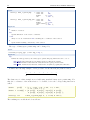
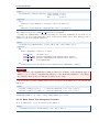
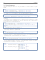
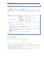
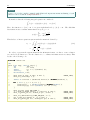
Consider the following example of a 1d problem over the interval [0, 1] with 8 vertices:
0
1
2
3
0
4
5
6
7
1
The cluster tree for this example is now build using standard binary space partitioning. For
this, the coordinates of the indices have to be defined, before the corresponding function is
called:
double
double
= { 0.0, 0.125, 0.25, 0.375, 0.5, 0.625,
0.75, 0.875, 1.0 };
* coord[8] = { & pos[0], & pos[1], & pos[2], & pos[3],
& pos[4], & pos[5], & pos[6], & pos[7] };
pos[8]
cluster_t ct1
= hlib_ct_build_bsp( 8, 1, coord, & info );
The resulting tree would then look as follows:
12
C Language Bindings
0, 1, 2, 3, 4, 5, 6, 7
4, 5, 6, 7
0, 1, 2, 3
0, 1
0
2, 3
1
2
4, 5
3
4
6, 7
5
6
7
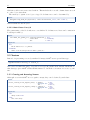
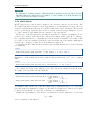
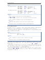
Now the cluster tree shall be computed with binary space partitioning and nested dissection.
Here, beside the coordinates, the connectivity of the indices is also needed. For this, we assume
that geometrically neighboured indices are also algebraically connected, which would result in
the following sparsity pattern of a corresponding matrix:

∗ ∗

∗ ∗ ∗



 ∗ ∗ ∗




∗
∗
∗




∗ ∗ ∗



∗ ∗ ∗ 



∗ ∗ ∗
∗ ∗

For the definition of such a matrix please refer to Section 3.4.1. The corresponding source for
this example is:
double
double
= { 0.0, 0.125, 0.25, 0.375, 0.5, 0.625,
0.75, 0.875, 1.0 };
* coord[8] = { & pos[0], & pos[1], & pos[2], & pos[3],
& pos[4], & pos[5], & pos[6], & pos[7] };
matrix_t
pos[8]
S
= ... /* see chapters below */
cluster_t ct2
= hlib_ct_build_bsp_nd( 8, 1, coord, S, & info );
Due to the interface nodes chosen by the nested dissection part of the algorithm, the resulting cluster tree has (mostly) a ternary structure. In the following tree, the coloured nodes
correspond to the interface vertices.
0, 1, 2, 3, 4, 5, 6, 7
0, 1, 2
0
1
4, 5, 6, 7
3
2
4
6, 7
5
6
7
Functions for Algebraic Clustering
If no geometrical data is available, an algebraic algorithm can be used, which is based only on
the connectivity described by a sparse matrix as it results from finite difference or finite element
13
3.2 Cluster Trees and Block Cluster Trees
methods. Since this does not always reflect the real data dependency in a grid, the resulting
clustering usually leads to a less efficient matrix arithmetic than the geometrical approach. As
in the previous case, the algebraic method can be combined with nested dissection.
Syntax
cluster_t hlib_ct_build_alg
( matrix_t
cluster_t hlib_ct_build_alg_nd ( matrix_t
S, int * info );
S, int * info );
Arguments
S
Sparse matrix defining connectivity between indices.
Due to the simple structure of the previous examples the resulting cluster trees using algebraic clustering would be identical.
3.2.1.3 Cluster Tree I/O
The tree structure of cluster trees can be exported in the PostScript format to a file by
Syntax
void hlib_ct_print_ps ( const cluster_t
ct,
const char
* filename,
int
* info );
Arguments
ct
Cluster tree to be printed.
filename
Name of the PostScript file to which ct shall be printed to.
3.2.2 Block Cluster Trees
The next building block for H-matrices are block cluster trees which represent a hierarchical
partitioning of the block indexset over which matrices are defined. They are constructed by
multiplying two cluster trees and choosing admissible nodes, e.g. nodes where the associated
block indexset allows a low-rank approximation in the matrix.
pro
Block cluster trees are represented in H-Lib by objects of type
typedef blockcluster_s * blockcluster_t;
3.2.2.1 Block Cluster Construction
Due to the definition of a block cluster tree two cluster trees are needed for the construction.
The actual building is performed by the routine
14
C Language Bindings
Syntax
blockcluster_t hlib_bct_build ( const cluster_t rowct,
const cluster_t colct,
int
* info );
Arguments
rowct
Cluster tree representing the row indexset of the block cluster tree.
colct
Cluster tree representing the column indexset of the block cluster tree.
The cluster trees given to hlib bct build can be identical.
Usually, the admissibility condition responsible for detecting admissible nodes in the block
cluster tree is chosen automatically based on the given cluster trees. The strategy can be
changed by the user with the function
Syntax
void hlib_set_admissibility ( const adm_t adm, const double eta );
Arguments
adm
Define admissibility condition to be either:
ADM
ADM
ADM
ADM
AUTO
STD MIN
STD MAX
WEAK
automatic choice,
standard admissibility with minimal cluster diameter,
standard admissibility with maximal cluster diameter or
weak admissibility.
eta
Scaling parameter for the distance between clusters in the admissibility condition.
Attention
Since changes to the admissibility condition can lead to a failure of the H-matrix approximation or to a reduced computational efficiency of the H-matrix arithmetic, only change
the default behaviour if you really know what you are doing.
To access the row and column cluster trees of a given block cluster tree, one can use the
functions
Syntax
cluster_t hlib_bct_row_ct
( const blockcluster_t bct, int * info );
cluster_t hlib_bct_column_ct ( const blockcluster_t bct, int * info );
which will return a copy of the corresponding cluster tree objects.
3.2.2.2 Block Cluster Tree Management Functions
A block cluster tree object is released by the function
Syntax
void hlib_bct_free ( blockcluster_t bct, int * info );
15
3.3 Vectors
which frees all resources associated with it. This includes the row and column cluster trees if
no other object uses them.
The memory footprint of an object of type block cluster tree can be determined by
Syntax
unsigned long hlib_bct_bytesize ( const blockcluster_t bct, int * info );
which returns the size in bytes.
3.2.2.3 Block Cluster Tree I/O
The partitioning of the block index set over which a block cluster tree lives can be written in
PostScript format by
Syntax
void hlib_bct_print_ps ( const blockcluster_t bct,
const char
* filename,
int
* info );
Arguments
bct
Block cluster tree to be printed.
filename
Name of the PostScript file bct will be printed to.
3.3 Vectors
pro
Instead of representing vectors by standard C arrays, H-Lib uses a special data type
typedef struct vector_s * vector_t;
One reason for this is the usage of special vector types in parallel environments. Furthermore,
pro
this data type gives H-Lib additional information to check the correctness of vectors, e.g. the
size.
3.3.1 Creating and Accessing Vectors
pro
Although vectors in H-Lib are not equal to arrays, they can be defined by such data:
Syntax
vector_t hlib_vector_import_array
( double
unsigned int
int
vector_t hlib_vector_import_carray ( complex_t
unsigned int
int
Arguments
arr
Array of size size.
size
Size of the array.
* arr,
size,
* info );
* arr,
size,
* info );
16
C Language Bindings
The arrays are directly used by the vector data type, i.e. changing the content of the arrays
also changes the content of the vector. This gives the possibility to efficiently access the vector
coefficients as it is shown in the following example:
unsigned int
n
= 1024;
double
* arr = (double *) malloc( sizeof(double) * n );
vector_t
x
= hlib_vector_import_array( arr, n, & info );
for ( i = 0; i < n; i++ )
arr[i] = i+1;
The coefficient i of the vector x would also equal i + 1 as does the array element arr[i+1].
pro
Such kind of vectors, e.g. scalar vectors, can also be created directly by H-Lib :
Syntax
vector_t hlib_vector_alloc_scalar ( unsigned int size, int * info );
vector_t hlib_vector_alloc_cscalar ( unsigned int size, int * info );
Arguments
size
Size of the scalar vector.
Since no external C array is available to access the elements of the vectors, this is accompro
plished by H-Lib functions. To get a specific element of a vector, the following two functions
can be used:
Syntax
double
hlib_vector_entry_get
( const vector_t
unsigned int
int
*
complex_t hlib_vector_centry_get ( const vector_t
unsigned int
int
*
Arguments
x
Vector to get element from.
i
Position of the element in the vector.
Similarly, the setting of a vector element is defined:
x,
i,
info );
x,
i,
info );
17
3.3 Vectors
Syntax
void hlib_vector_entry_set
( const vector_t
unsigned int
const double
int
*
void hlib_vector_centry_set ( const vector_t
unsigned int
const complex_t
int
*
x,
i,
f,
info );
x,
i,
f,
info );
Arguments
x
Vector to modify element in.
i
Position of the element to modify.
f
New value of the i’th element in x.
Two more functions are available to change a complete vector. First, all elements can be set
to a given constant value with
Syntax
void hlib_vector_fill ( vector_t x, const double
f, int * info );
void hlib_vector_cfill ( vector_t x, const complex_t f, int * info );
Arguments
x
Vector to be filled with constant value.
f
Value to be assigned to all elements of the vector.
Furthermore, the vector can be initialised to random values with
Syntax
void hlib_vector_fill_rand ( vector_t x, int * info );
3.3.2 Vector Management Functions
A copy of a vector is constructed by using the function
Syntax
vector_t hlib_vector_copy ( const vector_t x, int * info );
which returns a new vector object with it’s own data. If the original vector v corresponds to
a C array, the newly created vector does not represent this array but uses a new array.
The size of a vector can be determined by the function
Syntax
unsigned int hlib_vector_size ( const vector_t x, int * info );
Similarly, the memory size of a vector in bytes is obtained by
18
C Language Bindings
Syntax
unsigned long hlib_vector_bytesize ( const vector_t x, int * info );
Finally, vectors are released by using
Syntax
void hlib_vector_free ( vector_t x, int * info );
which frees all local memory of a vector. This does not apply to associated C arrays, e.g. if the
vector was constructed with hlib vector import array. There, the array has to be deleted
by the user.
3.3.3 Algebraic Vector Functions
pro
A complete set of function for standard algebraic vector operations is available in H-Lib .
In contrast to the vector copy function above, the following routine does not create a new
vector but copies the content of x to the vector y. For this, both vectors have to be of the
same type.
Syntax
void hlib_vector_assign ( vector_t y, const vector_t x, int * info );
Arguments
y
Destination vector of the assignment.
x
Source vector of the assignment.
Scaling a vector, e.g. the multiplication of each element with a constant is performed by
Syntax
void hlib_vector_scale ( vector_t x, const double
f, int * info );
void hlib_vector_cscale ( vector_t x, const complex_t f, int * info );
Summing up to vectors is implemented in the more general form
y := y + αx
with vectors x and y and the constant α. This operation is performed by the functions
Syntax
void hlib_vector_axpy
( vector_t
const double
const vector_t
int
*
void hlib_vector_caxpy ( vector_t
const complex_t
const vector_t
int
*
y,
alpha,
x,
info );
y,
alpha,
x,
info );
Real and complex valued dot-products can be computed with
19
3.3 Vectors
Syntax
double
hlib_vector_dot ( const vector_t x, const vector_t y, int * info );
complex_t hlib_vector_cdot ( const vector_t x, const vector_t y, int * info );
And the euclidean norm of a vector is returned by the function
Syntax
double hlib_vector_norm2 ( const vector_t x, int * info );
3.3.4 Vector I/O
In this section, functions for reading and saving vectors from/to files are discussed. Beside it’s
pro
own format, H-Lib supports several other vector formats.
3.3.4.1 SAMG
A special property of the SAMG format (see [Fra]) is the distribution of the data onto several
pro
files. Therefore, not the exact name of the file storing a vector has to be supplied to H-Lib ,
but the basename, e.g. without the file suffix.
Furthermore, only special vectors in a linear equations system are stored, namely the right
hand side and, if available, the solution of the system. To read these vectors, the following
functions are available:
Syntax
vector_t hlib_samg_load_rhs ( const char * basename,
int
* info );
vector_t hlib_samg_load_sol ( const char * basename,
int
* info );
In the same way, only these special vectors can be stored with
Syntax
void hlib_samg_save_rhs ( const vector_t
x,
const char
* basename,
int
* info );
void hlib_samg_save_sol ( const vector_t
x,
const char
* basename,
int
* info );
Due to the restrictions of the SAMG format, the vector has to be of a scalar type.
3.3.4.2 Matlab
pro
For now, H-Lib only supports the Matlab V6 file format (see [Mat]), e.g. without compression,
for dense and sparse vectors. All other Matlab data types, e.g. cells and structures, are not
supported. Both types of vectors will be converted to scalar vector types upon reading, e.g.
sparse vectors become dense. Conversely, only scalar vectors can be saved in the Matlab
format.
Since a vector in the Matlab file format is associated with a name, this name has to be
supplied to the corresponding I/O functions.
20
C Language Bindings
Syntax
vector_t hlib_matlab_load_vector ( const
const
int
void
hlib_matlab_save_vector ( const
const
const
int
char
char
* filename,
* vecname,
* info );
vector_t
v,
char
* filename,
char
* vecname,
* info );
Arguments
v
Scalar vector to be saved in Matlab format.
filename
Name of Matlab file containing the vector.
vecname
Name of the vector in the Matlab file.
3.3.4.3 HLIB
To be done.
3.4 Matrices
pro
All matrices in H-Lib are represented by the type
typedef struct matrix_s * matrix_t;
No difference is made between special matrix types, e.g. sparse matrices, dense matrices or
pro
H-matrices. Of course, inside H-Lib this distinction is done and the appropriate or expected
type is checked in each function.
pro
To use matrices in H-Lib three different ways are possible: import a matrix given by some
data structures, build a matrix or load a matrix from a file. The first method usually applies to
pro
sparse and dense matrices whereas H-matrices are normally build by H-Lib . These different
methods will be discussed in the following sections.
3.4.1 Importing Matrices from Data structures
Sparse Matrices
pro
Before using sparse matrices in H-Lib , they have to be imported to the internal representation.
For this, the sparse matrix is expected to be stored in compressed row storage or CRS format.
The CRS format consists of three arrays: colind, coeffs and rowind. The array colind
holds the column indices of each entry in the sparse matrix ordered according to the row, e.g.
at first all indices for the first row, then all indices for the second row and so forth. Here the
indices itself are numbered beginning from 0. In the same way, the array coeffs holds the
coefficients of the corresponding entries in the same order. Both array have dimension nnz,
i.e. the number of non-zero entries in the matrix. The last array, rowind, has dimension n + 1,
where n is the dimension of the matrix. It stores at position i − 1 the index to the colind
and coeffs array for the i’th row, e.g. the entries for the i’th row have the column indices
21
3.4 Matrices
colind[i − 1] . . . colind[i]-1 and the coefficients coeffs[i − 1] . . . coeffs[i]-1. The value
rowind[n] holds the number of non-zero entries.
As an example, the matrix


2 −1
−1 2 −1


S=

−1 2 −1
−1 2
of dimension 4 × 4 with 10 non-zero entries would result in the following arrays
int
rowind[5] = { 0, 2, 5, 8, 10 };
int
colind[10] = { 0, 1,
0, 1, 2,
double coeff[10] = { 2, -1, -1, 2, -1,
1, 2, 3,
-1, 2, -1,
2, 3 };
-1, 2 };
pro
To import a sparse matrix in CRS format into H-Lib , the following two functions can be
used:
Syntax
matrix_t hlib_matrix_import_crs
( const
const
const
const
const
const
const
int
matrix_t hlib_matrix_import_ccrs ( const
const
const
const
const
const
const
int
int
int
int
int
int
double
int
*
*
*
*
rows,
cols,
nnz,
rowind,
colind,
coeffs,
sym,
info );
rows,
int
int
cols,
int
nnz,
int
* rowind,
int
* colind,
complex_t * coeffs,
int
sym,
* info );
Arguments
rows,cols
Number of rows and columns of the sparse matrix.
nnz
Number of non-zero entries in the sparse matrix.
rowind, colind, coeffs
Arrays containing the sparse matrix in CRS format.
sym
If sym is non-zero, the sparse matrix is assumed to be symmetric.
The two routines only differ by the coefficient type of the sparse matrix which can either be
real or complex valued.
To finish the above described example by creating a matrix object from the constructed
arrays, one has to add a call to the corresponding function:
22
C Language Bindings
int
int
double
matrix_t
rowind[5] = { 0, 2, 5, 8, 10 };
colind[10] = { 0, 1,
0, 1, 2,
coeff[10] = { 2, -1, -1, 2, -1,
S;
1, 2, 3,
-1, 2, -1,
2, 3 };
-1, 2 };
S = hlib_import_crs( 4, 10, rowind, colind, coeffs );
Dense Matrices
Although, due to their high memory and computation overhead not the preferred type of
pro
matrix, H-Lib is also capable of handling dense matrices. As for sparse matrices, they have
to be imported for further usage.
When using dense matrices, the user has to keep in mind a very important aspect of their
storage:
Attention
pro
In contrast to the standard way in which C addresses dense matrices, H-Lib expects them
to be in column major format, e.g. stored column wise.
For example, the matrix
D=
1 2
3 4
has to be stored in an array as follows:
double
D[4] = { 1, 3, 2, 4 };
pro
The reason for this is the usage of LAPACK inside H-Lib . LAPACK is originally written in
Fortran and therefore uses column major format for all matrices.
pro
To import a dense matrix into H-Lib , the following two functions for real and complex
valued matrices are available:
Syntax
matrix_t hlib_matrix_import_dense
( const
const
const
const
int
matrix_t hlib_matrix_import_cdense ( const
const
const
const
int
int
rows,
int
cols,
double * D,
int
sym,
* info );
int
rows,
int
cols,
complex_t * D,
int
sym,
* info );
Arguments
rows, cols
The number of rows and columns of the dense matrix.
D
Array of dimension rows·cols in column major format containing the matrix coefficients.
sym
If sym is non-zero, the matrix is assumed to be symmetric.
23
3.4 Matrices
Importing the above defined matrix D is accomplished by
double
matrix_t
D[4] = { 1, 3, 2, 4 };
M
= hlib_matrix_import_dense( 2, 2, D, 0, & info );
3.4.2 Building H-Matrices
Before any H-matrix can be built, a corresponding block cluster tree has to be available, which
describes the partitioning of the block indexset of the matrix and defines admissible matrix
blocks. Please refer to Section 3.2.2 on how to get a suitable block cluster tree object.
3.4.2.1 Sparse Matrices
Sparse matrices are converted into H-matrices by using
Syntax
matrix_t hlib_matrix_build_sparse ( const blockcluster_t bct,
S,
const matrix_t
int
* info );
Arguments
bct
Block cluster tree defining partitioning of the block indexset of the sparse matrix.
S
Sparse matrix to be converted to an H-matrix.
Usually, the resulting H-matrix is an exact copy of the given sparse matrix. Although, due
to efficiency reasons, this equality is only valid with respect to machine precision.
3.4.2.2 Dense Matrices
Since dense matrices involve an unacceptable memory overhead, an H-matrix approximation
should not be built out of a given dense matrix but by constructing the data sparse approximation directly. This is accomplished by various algorithms.
Attention
The algorithms for computing a H-matrix approximation of a given dense matrix only work
for certain classes of matrices, e.g. coming from integral equations. They might not work
for general matrices. Be sure to check the applicability of the algorithms before using a
certain routine.
Adaptive Cross Approximation
Adaptive cross approximation or ACA is a technique which constructs an approximation to a
dense matrix by successively adding rank-1 matrices to the final approximation. For this, only
the matrix coefficients of the dense matrix are needed. These coefficients are given by the user
in the form of a coefficient function which evaluates certain parts of the global dense matrix.
The definition of these functions is as follows:
24
C Language Bindings
Syntax
typedef void (* coeff_fn_t)
( int n, int * rowcl, int m, int * colcl,
double * matrix, void * arg );
typedef void (* ccoeff_fn_t) ( int n, int * rowcl, int m, int * colcl,
complex_t * matrix, void * arg );
Arguments
n, rowcl
Number of row indices and the row indices in the for of an array at which the matrix shall be
evaluated.
m, colcl
Number of column indices and the column indices in the for of an array at which the matrix
shall be evaluated.
matrix
Array of dimension n·m at which the computed coefficients at the positions defined by rowcl
and colcl shall be stored in column major format.
arg
Optional argument to the coefficient function (see below).
pro
Different variants of ACA are available in H-Lib , each of them with it’s own advantages and
disadvantages. From a computation point of view interesting are the original formulation (see
[Beb00]) and advanced ACA (see [BG05]), ACA+ for short. These two have a linear complexity
in the dimension of the matrix and a quadratic complexity in the rank of the approximation.
This reduced complexity is possible since only a minor part of all coefficients is used inside
the algorithms. Unfortunately, this sometimes leads to errors in the approximation and hence,
both methods represent a heuristic approach. In practise however, at least ACA+ works quite
well.
To guarantee a certain approximation, one has to look at all coefficients of the matrix, which
then leads to a quadratic complexity in the size of the matrix block. This algorithm is called
ACAFull (see [BGH03]). Although the approximation can be guaranteed, the resulting rank
due to ACAFull might not be minimal, leading to an increase in the memory usage of the
resulting H-matrix.
Since an non-optimal rank might also happen with ACA or ACA+, each approximation is
truncated afterwards to ensure minimal memory overhead. This truncation procedure has a
computational complexity linear in the size of the matrix block and quadratic in the rank.
An optimal rank right from the beginning can be achieved with singular value decomposition
or SVD. Although this algorithm is not directly related to adaptive cross approximation, it is
pro
included in H-Lib . Unfortunately, SVD has a cubic complexity in the size of the matrix block
and is therefore only applicable for small matrices.
After defining a coefficient function, the following two routines can be used to construct a
H-matrix approximation to the corresponding dense matrix:
25
3.4 Matrices
Syntax
matrix_t hlib_matrix_build_coeff
( const
const
void
const
const
const
int
blockcluster_t
coeff_fn_t
*
lrapx_t
double
int
*
bct,
f,
arg,
lrapx,
eps,
sym,
info );
matrix_t hlib_matrix_build_ccoeff ( const
const
void
const
const
const
int
blockcluster_t
ccoeff_fn_t
*
lrapx_t
double
int
*
bct,
f,
arg,
lrapx,
eps,
sym,
info );
Arguments
bct
Block cluster tree over which the H-matrix shall be built.
f
Coefficient function defining dense matrix.
arg
Optional argument which will be passed to the coefficient function.
lrapx
Defines the type of low-rank approximation used in each admissible matrix block and can be
one of
LRAPX
LRAPX
LRAPX
LRAPX
SVD
ACA
ACAPLUS
ACAFULL
use
use
use
use
singular value decomposition
adaptive cross approximation
advanced adaptive cross approximation
adaptive cross approximation with full pivot search
Since an H-matrix is usually not an exact representation of the dense matrix but only an
pro
approximation, the accuracy for this approximation has to be specified. In H-Lib , this is
always done in a block-wise fashion. That means, that for a given dense matrix D and the
corresponding H-matrix A build out of D with an accuracy of ε ≥ 0 this accuracy only holds
for all block indexsets defined by leaves t × s in the block cluster tree:
kD|t×s − A|t×s k ≤ ε
but not necessarily for the matrices itself. This is a general property for all matrix operations
in the context of H-matrices.
As an example for building an H-matrix with adaptive cross approximation, we consider the
integral equation
Z 1
log |x − y|u(y)dy = f (x), x ∈ [0, 1]
0
R
with a suitable right hand side f : [0, 1] → . We are looking for the solution u : [0, 1] →
A standard Galerkin discretisation with constant ansatz functions ϕi , 0 ≤ i < n,
(
1 x ∈ ni , i+1
n
ϕi (x) =
0 otherwise
R.
26
C Language Bindings
leads to a linear equation system with the matrix coefficients
1Z 1
Z
aij
ϕi (x) log |x − y|ϕj (y)dydx
=
0
0
i+1
n
Z
=
i
n
j+1
n
Z
j
n
log |x − y|dydx
=: integrate a(i, j, n),
where integrate a denotes a function which evaluates the integral.
All of this is put together in the following example. There the coordinates of the indices
are set at the centre of the support of each basis function. The function coeff fn evaluates
integrate a at the given indices and writes the result into the given dense matrix. Please
note the access to D in column major form. The actual H-matrix is built using ACA+, which
is the recommended variant of adaptive cross approximation.
void coeff_fn ( int n, int * rowcl, int m, int * colcl,
double * D, void * arg ) {
int
i, j;
int * n = (int *) arg;
for ( i = 0; i < n; i++ )
for ( j = 0; j < m; j++ )
D[ j*n + i ] = integrate_a( rowcl[i], colcl[j], *n );
}
void build_matrix
int
int
double
**
cluster_t
blockcluster_t
matrix_t
() {
i, info;
n
= 1024;
coord[n] = (double**) malloc( sizeof(double*) * n );
ct;
bct;
A;
for ( i = 0; i < n; i++ ) {
}
}
coord[i]
= (double*) malloc( sizeof(double) );
coord[i][0] = (((double) i) + 0.5) / ((double) n);
ct = hlib_ct_build_bsp( n, 1, coord, & info );
bct = hlib_bct_build( ct, ct, & info );
A
= hlib_matrix_build_coeff( bct, coeff_fn, & n, LRAPX_ACAPLUS,
1e-4, 1, & info );
Remark
The above example is also implemented in the file examples/bem1d.c. There, also source
code for the function integrate a is available.
Hybrid Cross Approximation
To be done.
27
3.4 Matrices
3.4.3 Matrix Management
Using the following two function one can get the number of rows and columns of a specific
matrix.
Syntax
unsigned int hlib_matrix_rows
( const matrix_t A, int * info );
unsigned int hlib_matrix_columns ( const matrix_t A, int * info );
To obtain a copy of a block cluster tree associated with a matrix, the function
Syntax
blockcluster_t hlib_matrix_bct ( const matrix_t A, int * info );
is available.
In contrast to the copy operations so far, e.g. for cluster trees and block cluster trees, copying
a matrix always creates a new matrix. The copy can be either exact or up to a given accuracy.
Both operations are done with the functions:
Syntax
matrix_t hlib_matrix_copy
( const matrix_t A, int * info );
matrix_t hlib_matrix_copy_eps ( const matrix_t A, double eps, int * info );
Arguments
eps
Block-wise accuracy of the copy compared to A.
Deallocating a matrix is accomplished with
Syntax
void hlib_matrix_free ( matrix_t A, int * info );
Again, please remember to only use this function and not free to prevent undefined behaviour.
The memory usage of a specific function can be obtained by
Syntax
unsigned long hlib_matrix_bytesize ( const matrix_t A, int * info );
In some situations it might be necessary to access single matrix coefficients. For this the
following functions are available to return the entry Aij :
Syntax
double
hlib_matrix_entry_get
( const
const
const
int
complex_t hlib_matrix_centry_get ( const
const
const
int
matrix_t
unsigned int
unsigned int
A,
i,
j,
* info );
matrix_t
A,
unsigned int
i,
unsigned int
j,
* info );
28
C Language Bindings
Remark
For H-matrices obtaining a single coefficient has the complexity O (k log n), where k is the
maximal rank in the matrix and n the number of rows/columns of A. It should therefore
only be used when absolutely necessary.
3.4.4 Matrix Norms
pro
H-Lib supports two basic norms for matrices: the Frobenius and the spectral norm. The
Frobenius norm plays a crucial role in the approximation of each matrix block, where the local
accuracy is always meant with respect to the Frobenius norm of the local matrix. The spectral
norm, e.g. the largest eigenvalue, gives a better overview of the global approximation, e.g. how
good the computed, approximate inverse compares to the exact inverse.
In the case of the spectral norm, the largest eigenvalue is computed by using the Power
iteration (see [GL96]). Since this is also only an approximate method and due to efficiency
pro
the computational effort for computing the norm is restricted in H-Lib , the result of this
procedure does not necessarily represent the exact spectral norm of the matrix. Although in
practise, the convergence behaviour for most matrices is quite well.
Computing the Frobenius and the spectral norm for a single matrix is done by the following
two functions:
Syntax
double hlib_matrix_norm_frobenius ( const matrix_t
double hlib_matrix_norm_spectral ( const matrix_t
A, int * info );
A, int * info );
Furthermore, if the matrix A is not ill-conditioned the spectral norm of A−1 can be obtained
with
Syntax
double hlib_matrix_norm_spectral_inv ( const matrix_t
A, int * info );
To compute the norm of the difference kA − Bk between two matrices A and B in the
Frobenius or the spectral norm, the functions
Syntax
double hlib_matrix_norm_frobenius_diff ( const
const
int
double hlib_matrix_norm_spectral_diff ( const
const
int
matrix_t
matrix_t
A,
B,
* info );
matrix_t
A,
matrix_t
B,
* info );
are available. Here, in the case of the Frobenius norm, both matrices have to be of the same
type and, if they are H-matrices, defined over the same block cluster tree. This does not apply
to the spectral norm since it only relies on matrix vector multiplication.
Finally, the approximation of the inverse of a matrix A by another matrix B, e.g. the norm
kI − ABk2
can be computed by the function
29
3.4 Matrices
Syntax
double hlib_matrix_norm_inv_approx ( const matrix_t
A,
B,
const matrix_t
int
* info );
3.4.5 Matrix I/O
pro
Various matrix file formats are supported by H-Lib which will be discussed in this section.
3.4.5.1 SAMG
The SAMG package (see [Fra]) defines a matrix file format for sparse matrices and vectors in a
linear equations system, namely the solution and the right-hand-side. Im- and exporting these
pro
pro
objects is supported by H-Lib . Unfortunately, H-Lib is not able to handle coupled systems
saved in this format.
A special property of the SAMG format is the distribution of the data onto several files.
pro
Therefore, not the exact name of the file storing a matrix has to be supplied to H-Lib , but
the basename, e.g. without the file suffix.
Syntax
matrix_t hlib_samg_load_matrix ( const char
int
void
* basename,
* info );
hlib_samg_save_matrix ( const matrix_t
S,
const char
* basename,
int
* info );
Arguments
S
Sparse matrix to store in SAMG format.
basename
Name of the matrix file without suffix.
3.4.5.2 Matlab
pro
For now, H-Lib only supports the Matlab V6 file format (see [Mat]), e.g. without compression,
for dense and sparse matrices. All other Matlab data types, e.g. cells and structures, are not
supported. Furthermore, H-matrices can not be saved in the Matlab format.
Since a matrix in the Matlab file format is associated with a name, this name has to be
supplied to the corresponding I/O functions.
30
C Language Bindings
Syntax
matrix_t hlib_matlab_load_matrix ( const char
const char
int
void
* filename,
* matname,
* info );
hlib_matlab_save_matrix ( const matrix_t
M,
const char
* filename,
const char
* matname,
int
* info );
Arguments
M
Sparse or dense matrix to save to filename
filename
Name of Matlab file to load/save matrix from/to.
matname
Name of the matrix in the Matlab file.
3.4.5.3 H-Lib
pro
Since H-matrices can not be stored in an efficient way in current matrix formats, H-Lib defines
it’s own file format for matrices. This format also supports sparse and dense matrices.
The corresponding functions to load and save matrices from/to files are:
Syntax
matrix_t hlib_hformat_load_matrix ( const char
int
void
* filename,
* info );
A,
hlib_hformat_save_matrix ( const matrix_t
const char
* filename,
int
* info );
Arguments
M
Matrix to save to filename
filename
Name of file to load/save matrix from/to.
3.4.5.4 PostScript
pro
Matrices in H-Lib can also be printed in PostScript format. Here various options are available
to define the kind of data in the resulting image:
MATIO SVD
print singular value decomposition in each block
MATIO ENTRY
print each entry of matrix
MATIO PATTERN print sparsity pattern (non-zero entries)
These options can also be combined by boolean “or”, e.g. to print the SVD and the sparsity
pattern the combination MATIO SVD || MATIO PATTERN is used. By default, only the structure
of the matrix is printed. There, different kind of blocks are marked by different colours:
31
3.5 Algebra
dense matrix blocks
admissible low-rank matrix blocks
non-admissible low-rank matrix blocks (see ???)
sparse matrix blocks
no matrix block exists
In addition, special information about each block is printed. For dense and sparse blocks the
dimension is shown in the lower left corner. For low-rank blocks, there the rank of the matrix is
printed. If SVD is chosen to be printed for each block the actual rank of the matrix is printed
at the centre of each block. For low-rank matrices this is only shown, if the SVD-rank differs
from the rank of the matrix. An example for a sparse matrix and a dense matrix (with and
without SVD) looks like:
21
15
10
21
21
4
21
21
21
7
15 7
21
7
15
28
28
10
10
9
6
28
10
21
4
7
28
10
21
21
10
9
6
7
21
10
15 21
21
36
10
5
10
6
5
15
6
12
6
4
21
15
21
4
10
21
21
21
21
8
8
15
21
12
8
10
7
21
15
15 21
36
10
5
6
21
10
4
7
6
5
15
6
12
15 7
21
7
15
28
10
10
28
21
5
21
6
4
15 21
10
12
36
10
10
9
6
5
15
6
12
6
21
8
8
15
28
28
10
21
5
21
6
4
15 21
21
4
21
10
28
21
10
15
12
36
10
5
15
6
21
15
21
28
10
12
10
15
21
4
9
6
36
10
5
21
10
10
28
15
21
15
10
21
21
10
28
21
8
6
21
4
21
7
8
21
10
6
28
12
8
10
5
15
6
21
12
10
5
15
6
10
6
15
5
6
10
4
6
21
15
5
21
10
21
9
19
36
12
8
12
6
15
8
8
21
12
8
12
6
21
8
8
15
15 7
21
7
28
19
8
10
9
6
7
15
7
10
21
21
4
6
36
10
5
21
10
10
28
15 7
21
21
15
8
8
21
12
8
15
21
21
4
21
7
10
28
15
12
15
9
6
7
21
4
8
8
10
15
21
15
6
21
10
7
10
7
21
21
4
7
21
21
7
19
8
10
6
15
5
6
10
9
6
7
4
6
21
15
5
21
10
21
7
10
7
19
36
12
15
8
8
21
8
7
8
21
8
8
15
21
36
21
6
9
12
10
10
15 21
21
5
6
4
10
6
5
15
6
15
21
10
21
28
10
10
36
28
10
21
8
21
8
8
15
21
36
4
21
21
12
6
9
12
10
7
21
5
6
4
15
15 21
10
6
5
15
6
10
15 7
7
21
7
15
10
21
4
7
28
10
10
36
28
10
21
21
12
7
12
21
8
8
8
15
6
9
19
21
5
6
4
10
21
28
10
15 21
21
15
10
21
28
12
6
5
15
6
10
10
21
4
21
21
12
21
8
8
8
15
6
9
21
5
6
4
21
21
19
7
10
7
28
10
21
8
6
15
8
8
21
5
6
6
9
36
10
21
15 4
6
10
21 5
21
15
8
6
15
21
5
6
10
8
8
10
21
21
4
21
12
21
10
15
21
4
6
5
21
28
10
28
6
9
10
36
21
10
28
15
21
12
10
5
6
10
7
21
21
7
21
15 4
10
21 5
6
7
10
21
15
21
21
4
21
7
12
21
10
15 7
21
4
6
5
21
7
28
10
28
10
36
21
10
28
15 7
21
15
225
19
12
15
8
8
8
21
6
9
12
6
15
5
6
10
10
21
21
4
21
10
21
15
10
21
28
19
15
8
8
8
21
6
9
6
15
5
6
10
7
12
4
7
10
36
10
7
12
6
21
12
28
15
15
15
15
15 21
15 7
15
10
12
10
7
21
15
10
21
7
15
21
21
4
21
7
10
7
28
The actual PostScript image is finally produced by the function
Syntax
void hlib_matrix_print_ps ( const matrix_t
A,
const char
* filename,
const int
options,
int
* info );
Arguments
A
Matrix to be printed.
filename
Name of the PostScript file A shall be printed to.
options
Combination of MATIO options or 0.
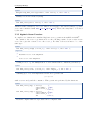
3.5 Algebra
3.5.1 Basic Algebra Functions
3.5.1.1 Matrix Vector Multiplication
pro
The multiplication of a matrix A with a vector x is implemented in H-Lib as the update of
the destination vector y as:
y := βy + αAx.
The special cases with β = 0 or α = 0 are also handled efficiently. Furthermore, the multiplipro
cation with the adjoint matrix AH is supported by H-Lib . The type of operation is chosen by
a parameter of type
32
C Language Bindings
typedef enum { OP_NORM, OP_ADJ } matop_t;
where OP NORM corresponds to Ax and OP ADJ to AH x.
The following two functions above computation. Both routines can handle real and complex
valued matrices and vectors. The difference in the name only applies to the type of the constant
factors.
Syntax
void hlib_matrix_mulvec
( const
const
const
const
void hlib_matrix_cmulvec ( const
const
const
const
double
matrix_t
double
matop_t
alpha,
A,
const vector_t x,
beta, vector_t
y,
matop, int
* info );
complex_t
matrix_t
complex_t
matop_t
alpha,
A,
const vector_t x,
beta, vector_t
y,
matop, int
* info );
Arguments
A
Sparse, dense or H-matrix to multiply with.
x
Argument vector of dimension hlib matrix columns(A)
hlib matrix rows(A) in the case of AH x.
if
Ax
is
performed
and
y
Result vector of the multiplication of dimension hlib matrix rows(A) if Ax is performed and
hlib matrix columns(A) in the case of AH x.
alpha,beta
Scaling factors for the matrix-vector product and the destination vector.
matop
Defines multiplication with A or adjoint matrix of A.
3.5.1.2 Matrix Addition
pro
The sum of two matrices A and B in H-Lib is defined as
B := αA + βB
with α, β ∈
R or α, β ∈ C depending on using real or complex arithmetic.
The two matrices for the matrix addition have to be compatible, i.e. of the same format. For
example, it is not possible to add a sparse and a H-matrix. Furthermore, H-matrices have to
be defined over the same block cluster tree.
When summing up H-matrices, this is done up to a given accuracy. As usual, this accuracy
is block-wise. Sparse and dense matrices are always added exactly.
33
3.5 Algebra
Syntax
void hlib_matrix_add
( const double
const double
const double
alpha, const matrix_t A,
beta, matrix_t
B,
eps,
int
* info );
void hlib_matrix_cadd ( const complex_t
const complex_t
const double
alpha, const matrix_t A,
beta, matrix_t
B,
eps,
int
* info );
Arguments
A, B
Matrices to be added. The result will be stored in B.
alpha, beta
Additional scaling factors for both matrices.
eps
Block-wise accuracy of the addition in the case of H-matrices.
3.5.1.3 Matrix Multiplication
Matrix multiplication can only be performed with dense and H-matrices. Furthermore, if the
arguments are H-matrices, they have to have compatible cluster trees, e.g. for the product
C := A · B
the column cluster tree of A and the row cluster tree of B must be identical. This also applies to
the row cluster trees of A and C as well as for the column cluster trees of B and C. Otherwise
the function exits with a corresponding error code.
The multiplication itself is defined as the update to a matrix C with additional scaling
arguments:
C := αAB + βC.
The matrices A and B can also be transposed or conjugate transposed in the case of complex
valued arithmetic.
34
C Language Bindings
Syntax
void hlib_matrix_mul
( const
const
const
const
const
void hlib_matrix_cmul ( const
const
const
const
const
double
matop_t
matop_t
double
double
alpha,
matop_A,
matop_B,
beta,
eps,
const matrix_t
const matrix_t
matrix_t
int
*
A,
B,
C,
info );
complex_t
matop_t
matop_t
complex_t
double
alpha,
matop_A,
matop_B,
beta,
eps,
const matrix_t
const matrix_t
matrix_t
int
*
A,
B,
C,
info );
Arguments
A, B
Dense or H-matrices used as factors for the matrix multiplication.
matop A, matop B
Defines multiplication with A, B or the corresponding adjoint matrices AH and BH .
C
Dense or H-matrix containing the result of the matrix multiplication.
alpha, beta
Additional scaling arguments for the product and the destination matrix.
eps
Block-wise accuracy of the H-arithmetic during the matrix multiplication.
3.5.1.4 Matrix Inversion
pro
In H-Lib , the inverse of a matrix is computed using Gaussian elimination. This method is
implemented for dense and H-matrices, e.g. sparse matrices can not be inverted.
The following functions computes the corresponding inverse to the given matrix A, which
will be overwritten by the result.
Syntax
void hlib_matrix_inv ( matrix_t
A,
const double eps,
int
* info );
Arguments
A
Dense or H-matrix to be inverted. A will be overwritten by the result.
eps
Block-wise accuracy of the H-arithmetic during the inversion.
The quality of the computation can be checked by computing the spectral norm of kI −ABk,
with B being the approximate inverse of A, by using function hlib matrix inv approx (see
Section 3.4.4).
An alternative algorithm is the LU decomposition of a matrix, which allows the fast evaluation of the inverse operator. Since not the real inverse is computed, the decomposition can
not be used for matrix arithmetic, e.g. matrix multiplication.
Function hlib matrix inv lu computes the LU decomposition and overwrites A with a
matrix representing the inverse of the factors, e.g. (LU )−1 . Therefore, evaluating A afterwards
corresponds to A−1 and not A.
35
3.5 Algebra
Syntax
void hlib_matrix_inv_lu ( matrix_t
A,
const double eps,
int
* info );
Arguments
A
Dense or H-matrix to be decomposed using LU factorisation. A will be overwritten with the
inverse of the factorisation result.
eps
Block-wise accuracy of the H-arithmetic during the LU decomposition.
Remark
When using LU decomposition to compute the inverse of an H-matrix based upon a sparse
matrix, nested dissection for the cluster tree construction (see Section 3.2.1.2) leads to an
improved computational efficiency of the algorithm.
3.5.2 Solving Linear Systems
Various iterative methods are available to solve a linear system: Richardson-, CG-, BiCGStaband GMRES iteration (see [Hac93], [vdV92] and [SS86]). Furthermore, all of these methods
can be preconditioned with an appropriated matrix, e.g. by the inverse of a matrix.
Before a system can be solved, a solver object has to be created. For the Richardson iteration,
this is accomplished by the function
Syntax
solver_t hlib_solver_rich ( const int
const double
const double
int
*
maxit,
abs_red,
rel_red,
iter );
Arguments
maxit
Maximal number of iterations.
abs red
Absolute reduction of the l2 -norm of the residual or negative, if this reduction shall not be
checked.
rel red
Relative reduction of the l2 -norm of the residual compared to the initial norm of the residual
or negative, if this reduction shall not be checked.
Similarly, for the CG- and the BiCG-Stab iteration the functions are
Syntax
solver_t hlib_solver_cg
( const int
const double
const double
int
*
maxit,
abs_red,
rel_red,
iter );
solver_t hlib_solver_bicgstab ( const int
const double
const double
int
*
maxit,
abs_red,
rel_red,
iter );
36
C Language Bindings
In the case of the GMRES-Iteration an additional parameter is expected which describes
the dimension of the local Krylov subspace, e.g. when to restart.
Syntax
solver_t hlib_solver_gmres ( const
const
const
const
int
int
int
double
double
restart,
maxit,
abs_red,
rel_red,
* iter );
Arguments
restart
Defines the number of iteration steps after which a restart is performed during the GMRESiteration, e.g. the dimension of the constructed Krylov-subspace.
This solver object can than be used with the actual solution functions. Using the above
iteration methods to solve
Ax = b
without preconditioning is done by
Syntax
void hlib_solve
( const solver_t
const matrix_t
vector_t
const vector_t
int
solver,
A,
x,
b,
* info );
Arguments
solver
Defines iteration method.
A, x, b
Define linear equation system.
If a preconditioner is available, one can use:
Syntax
void hlib_solve_precond
( const solver_t
const matrix_t
vector_t
int
solver,
A,
const matrix_t
x,
const vector_t
* info );
W,
b,
Arguments
W
Preconditioner to the linear equation system.
3.6 Miscellaneous Functions
pro
The following functions are mostly included in H-Lib for convenience and are usually available
by other libraries or even the operating system itself.
37
3.6 Miscellaneous Functions
3.6.1 Quadrature Rules
pro
Since H-Lib is capable of discretising integral equations, different quadrature rules are implemented as part of the computations. These rules are also exported so that external routines
can benefit from them.
3.6.1.1 Gaussian Quadrature
Quadrature rules for Gaussian quadrature of order n over the interval [0, 1] are constructed by
the function
Syntax
void
hlib_gauss_quadrature_1d ( const unsigned int order,
double * points, double * weights,
int
* info );
Arguments
n
Order of the quadrature.
points
Array of size order where the quadrature points will be stored.
weights
Array of size order where the quadrature weights will be stored.
3.6.1.2 Quadrature Rules for Triangles
pro
H-Lib also provides quadrature rules for the integration over a pair of triangles, e.g. when
computing integral equations on a surface grid. These rules were developed by Stefan Sauter
(see [SS04]). There different rules apply to different cases of triangle interaction:
same triangle
common edge
common vertex
separated triangles
The quadrature points are build for each triangle individually, where the triangle itself is
the standard 2d simplex
(0,1)
(0,0)
(1,0)
Therefore, you have to transform the computed coordinates to your triangles.
Computing the quadrature rules for equal triangles in done with
C Language Bindings
38
Syntax
void
hlib_sauter_quadrature_eq ( const unsigned int order,
double
* tri1_pts[2],
double
* tri2_pts[2],
double
* weights,
int
* info );
Arguments
order
Order of the quadrature.
tri1 pts, tri2 pts
Array where the 2d quadrature coordinates for both triangles are stored. The array have to be
of size 6 · order4 .
weights
Array of size 6 · order4 holding the quadrature weights.
Similar defined are the functions for triangles with a common edge, a common vertex or
separated triangles:
Syntax
void
hlib_sauter_quadrature_edge ( const unsigned int order,
double
* tri1_pts[2],
double
* tri2_pts[2],
double
* weights,
int
* info );
Arguments
tri1 pts, tri2 pts, weights
Arrays of size 5 · order4 .
Syntax
void
hlib_sauter_quadrature_vtx ( const unsigned int order,
double
* tri1_pts[2],
double
* tri2_pts[2],
double
* weights,
int
* info );
Arguments
tri1 pts, tri2 pts, weights
Arrays of size 2 · order4 .
Syntax
void
hlib_sauter_quadrature_sep ( const unsigned int order,
double
* tri1_pts[2],
double
* tri2_pts[2],
double
* weights,
int
* info );
Arguments
tri1 pts, tri2 pts, weights
Arrays of size order4 .
39
3.7 Examples
3.6.2 Measuring Time
pro
Two types of time can be measured by H-Lib : the CPU time and the wall clock time. The
first corresponds to the time spent by the program actually computing things. This type of
time has the advantage, that the load on the machine does not have any influence on the value
of the time. In contrast to this, the wall clock time is the actual time as measured by a real
clock. This type of time is dependent on the load on the computer system and therefore might
be different between two runs of the program.
The actual functions to obtain both types are:
Syntax
double hlib_walltime ();
double hlib_cputime ();
The absolute value of these functions is normally not usable. Only the difference between two
measurements returns the passed time.
3.7 Examples
pro
In the following two typical example for the usage of H-Lib are discussed in more detail.
3.7.1 Sparse Linear Equation System
In this section a linear equation system
Sx = b
with a sparse matrix S and a right hand side b is considered. Such a system usually occures
in the context of finite difference or finite element discretisations. The linear system itself is
provided in the form of a SAMG dataset with the basename “samg matrix” (see Section 3.3.4.1
and Section 3.4.5.1).
Remark
The complete example with additional output statements and timing of each function is
available in examples/crsalg.c. A similar example with geometrical clustering can be
found in examples/crsgeom.c.
Initialisation and Data Import
pro
At first, in the example below, H-Lib is initialised and the data is imported from the corresponding files:
40
C Language Bindings
1
#include <hlib-c.h>
2
3
4
5
6
7
int
main ( int argc, char ** argv ) {
matrix_t
S;
vector_t
b, x;
int
n, info;
char
mtx_data[] = "samg_matrix";
8
hlib_init( & argc, & argv, & info );
CHECK_INFO;
9
10
S = hlib_samg_load_matrix( mtx_data, & info );
hlib_matrix_print_ps( S, "crsalg_S.ps",
MATIO_PATTERN, & info );
b = hlib_samg_load_rhs(
mtx_data, & info );
x = hlib_matrix_col_vector( S, & info );
CHECK_INFO;
11
12
CHECK_INFO;
CHECK_INFO;
CHECK_INFO;
The sparse matrix is imported into the variable S at line 9. There, only the basename of
the SAMG file is provided without any suffix. This matrix is afterwards printed to the file
crsalg S.ps in PostScript format (see Section 3.4.5.4). As the option MATIO PATTERN is given,
only the pattern of non-zero matrix elements is printed.
After importing the matrix, the right hand side b is read from the SAMG file at line 11.
Again, only the basename is given to identify the corresponding file. The solution vector x is
then constructed by asking the matrix S for a suitable vector (see Section ??).
The macro CHECK INFO looks at the value of the variable info after each function call to
pro
H-Lib and tests whether an error occured. The definition of CHECK INFO is as follows:
#define CHECK_INFO
{ if ( info != NO_ERROR ) \
{ char buf[1024]; hlib_error_desc( buf, 1024 ); \
printf( "\n%s\n\n", buf ); exit(1); } }
There, the complete error message is copied into the string buf and printed to the standard
output. Afterwards, the program is aborted.
Coming back to the linear system, since the complete data is now available, one could solve
it. For this, a solver object (see Section 3.5.2 has to be created, which is in this case a GMRES
solver with a restart after 10 iteration steps and at most 1000 iterations. Furthermore, the
residual should be reduced until a norm of 10−8 was reached. The system can then be solved
with hlib solve.
solver_t gmres = hlib_solver_gmres( 10, 1000, 1e-8,
0, & info );
14 hlib_solve( gmres, S, x, b, & info );
13
CHECK_INFO;
CHECK_INFO;
LU Factorisation for Preconditioning
Since the standard iteration process is usually far to costly, a suitable preconditioner based
on the H-matrix technique is constructed to speed up the process. At first, this is accomplished by using LU factorisation in combination with nested dissection (see Section 3.2.1.2
and Section 3.5.1.4).
But before the matrix can be factorised, it has to be converted to an H-matrix. For this,
one needs a cluster tree and a block cluster tree. Since no geometrical data is available in this
41
3.7 Examples
example, both objects are constructed algebraically with the functions hlib ct build alg nd
and hlib bct build:
15
16
cluster_t ct = hlib_ct_build_alg_nd( S, & info );
hlib_ct_print_ps( ct, "crsalg_ct_nd.ps", & info );
CHECK_INFO;
CHECK_INFO;
17
18
blockcluster_t bct = hlib_bct_build( ct, ct, & info );
hlib_bct_print_ps( bct, "crsalg_bct_nd.ps", & info );
CHECK_INFO;
CHECK_INFO;
At line numbers 17 and 19, the two trees are printed to the files crsalg ct nd.ps and
crsalg bct nd.ps, respectively.
Now the sparse matrix S can be converted to an H-matrix, which then is factorised into LU
factors with a blockwise precision of 10−4 :
19
20
matrix_t A = hlib_matrix_build_sparse( bct, S, & info ); CHECK_INFO;
hlib_matrix_print_ps( A, "arsalg_A_nd.ps",
MATIO_PATTERN, & info );
CHECK_INFO;
21
22
hlib_matrix_inv_lu( A, 1e-4, & info );
hlib_matrix_print_ps( A, "crsalg_LU_nd.ps",
MATIO_SVD, & info );
23
CHECK_INFO;
CHECK_INFO;
printf( " size of LU factor = %.2f MB\n",
((double) hlib_matrix_bytesize( A, & info )) / (1024.0 *1024.0) );
The matrix A is overwritten with its LU factorisation, or, to be precise, with the inverse of its
LU factorisation. Both matrices are printed to PostScript files at the lines 21 and 23. In the case
of the factorised matrix, the singular value decomposition of the matrix is printed as chosen by
the parameter MATIO SVD. The size of the LU factors is determined by hlib matrix bytesize
and printed at line 24.
The above equation system can now be solved with the inverse of the LU factorisation of A
as a preconditioner:
24
hlib_solve_precond( gmres, S, A, x, b, & info );
CHECK_INFO;
Again, the GMRES iteration is used.
Finally, the locally created objects, e.g. the cluster tree, the block cluster tree and the
H-matrix can be deleted:
25
26
27
hlib_matrix_free( A, & info );
hlib_bct_free( bct, & info );
hlib_ct_free( ct, & info );
CHECK_INFO;
CHECK_INFO;
CHECK_INFO;
Matrix Inversion for Preconditioning
An alternative procedure for solving the above system fast is using matrix inversion . Again,
before the matrix can be inverted, a cluster tree and a block cluster tree have to be constructed.
Nested dissection, as it was used for LU decomposition, is not a suitable technique for matrix
inversion (see Section 3.2.1.2). Hence, standard algebraic partitioning functions are called:
42
C Language Bindings
28
29
cluster_t ct = hlib_ct_build_alg( S, & info );
hlib_ct_print_ps( ct, "crsalg_ct.ps", & info );
CHECK_INFO;
CHECK_INFO;
30
31
blockcluster_t bct = hlib_bct_build( ct, ct, & info );
hlib_bct_print_ps( bct, "crsalg_bct.ps", & info );
CHECK_INFO;
CHECK_INFO;
Converting the sparse matrix into an H-matrix is done by the same function as before. Only
the matrix inversion is now performed by hlib matrix inv:
32
33
matrix_t A = hlib_matrix_build_sparse( bct, S, & info );
hlib_matrix_print_ps( A, "crsalg_A.ps",
MATIO_PATTERN, & info );
CHECK_INFO;
CHECK_INFO;
34
35
hlib_matrix_inv( A, 1e-4, & info );
CHECK_INFO;
hlib_matrix_print_ps( A, "crsalg_I.ps", MATIO_SVD, & info ); CHECK_INFO;
36
printf( " size of Inverse = %.2f MB\n",
((double) hlib_matrix_bytesize( A, & info )) / (1024.0 *1024.0) );
Again, A is overwritten by its inverse matrix. Both matrices are also printed to PostScript
files, whereby for the inverse matrix the singular value decomposition of each matrix block is
shown.
The linear equation system is then solved as in the previous case:
37
hlib_solve_precond( gmres, S, A, x, b, & info );
CHECK_INFO;
And also the deletion of all created objects is done by the same functions:
38
39
40
hlib_matrix_free( A, & info );
hlib_bct_free( bct, & info );
hlib_ct_free( ct, & info );
CHECK_INFO;
CHECK_INFO;
CHECK_INFO;
Finalisation
pro
Finally, all other objects which where created at the beginning should be released and H-Lib
be finished:
41
42
43
44
hlib_vector_free(
hlib_vector_free(
hlib_matrix_free(
hlib_solver_free(
x, & info );
b, & info );
S, & info );
gmres, & info );
45
hlib_done( & info );
CHECK_INFO;
CHECK_INFO;
CHECK_INFO;
CHECK_INFO;
CHECK_INFO;
3.7.2 Integral Equation
The following example was already used in Section 3.4.2 to demonstrate the conversion of
dense matrices to H-matrices. Now it should be discussed in more detail in the context of a
complete example.
43
3.7 Examples
Remark
Source code for the complete example with additional output statements and timing of each
function can be found in examples/bem1d.c.
Remember, that the following integral equation is considered:
Z 1
log |x − y|u(y)dy = f (x), x ∈ [0, 1]
0
R
Here, the function u : [0, 1] →
for a given right hand side f : [0, 1] →
discretisation uses constant ansatz functions ϕi , 0 ≤ i < n
(
1 x ∈ [ ni , i+1
n ]
ϕi (x) =
0 otherwise
R.
The Galerkin
This leads to a linear equations system with the matrix A defined by
Z 1Z 1
aij =
ϕi (x) log |x − y|ϕj (y)dydx
0
i+1
n
Z
=
i
n
(3.1)
0
j+1
n
Z
j
n
log |x − y|dydx
In order to represent the system matrix in the H-matrix format, one has to create a cluster
tree and a block cluster tree. For the cluster tree, coordinate informations are necessary. This
leads to the following code:
#include <hlib-c.h>
int
main ( int argc, char ** argv ) {
int
info;
1
int
n = 1024;
2
double
h = 1.0 / ((double) n);
3
cluster_t
ct;
4
blockcluster_t bct;
5
6
7
hlib_init( & argc, & argv, & info );
hlib_set_verbosity( 2 );
8
double ** vertices = (double**) malloc( n * sizeof(double*) );
9
10
11
CHECK_INFO;
for ( int i = 0; i < n; i++ ) {
}
vertices[i]
= (double*) malloc( sizeof(double) );
vertices[i][0] = h * ((double) i) + (h / 2.0);
12
13
14
hlib_set_bsp_type( BSP_CARD );
ct = hlib_ct_build_bsp( n, 1, vertices, & info );
hlib_ct_print_ps( ct, "bem1d_ct.ps", & info );
CHECK_INFO;
CHECK_INFO;
15
16
17
hlib_set_admissibility( ADM_STD_MIN, 2.0 );
bct = hlib_bct_build( ct, ct, & info );
hlib_bct_print_ps( bct, "bem1d_bct.ps", & info );
CHECK_INFO;
CHECK_INFO;
44
C Language Bindings
The dimension of the problem is defined by the variable n, which also defines the stepsize h of
the discretisation. Evaluationg info is again done by the macro CHECK INFO which is defined
as in the previous section.
pro
After initialising H-Lib , the coordinate
information is created at the lines 8 to 11. At this,
the middle of each interval ni , i+1
was
chosen
as the coordinate for the corresponding vertex
n
i.
With this, the cluster tree can be created as it is done at line 13. Here, the clustering
strategy was explicitly set to cardinality balanced clustering (see Section 3.2.1.2). The tree is
afterwards printed to the file bem1d ct.ps in PostScript format.
Finally, one can construct the block cluster tree. Again, the type of construction is explicitly
set in the form of a strong admissibility condition with a scaling parameter of size 2 (see also
Section 3.2.2.1).
Attention
Choosing the clustering strategy as well as the admissibility condition is only suggested,
if the user is absolutely sure, that the corresponding options really apply to the problem
under consideration. Otherwise, the H-matrix technique might fail, e.g. a desired accuracy
is unreachable or the computational complexity is to high. When in doubt, use the standard
settings.
After the partitioning of the block indexset in the form of the block cluster tree is computed,
the actual H-matrix can be build. For this, adaptive cross approximation (or ACA, see Section 3.4.2) is used in this example. ACA needs a matrix coefficient function, which computes
the matrix entries for given index pairs. In our case, this function is given by (3.1), which,
after evaluating the integral, translates into the following code:
void kernel ( int n, int * rowcl, int m, int * colcl,
double * matrix, void * arg ) {
int
rowi, colj;
double h = *((double*) arg);
for ( colj = 0; colj < m; colj++ ) {
int idx1 = colcl[colj];
for ( rowi = 0; rowi < n; rowi++ ) {
int
idx0 = rowcl[rowi];
double value;
double d = h * ( fabs( (double) (idx0-idx1) ) - 1.0 );
if ( idx0 == idx1 )
value = -1.5*h*h + h*h*log(h);
else {
value = ( - 1.5*h*h + 0.5*(d+2.0*h)*(d+2.0*h)*log(d+2.0*h)
- (d+1.0*h)*(d+1.0*h)*log(d+1.0*h) );
if ( fabs(d) > 1e-8 )
value += 0.5*(d)*(d)*log(d);
}
matrix[(colj*n) + rowi] = -value;
}
}
}
45
3.7 Examples
The arguments n, rowcl, m and colc define a submatrix of dimension n×m with row and column
indices stored in rowcl and colcl. The coefficients should be stored in column wise ordering
in matrix. The additional argument arg contains the h stepwidth of the discretisation.
Equipped with the coefficient function, the code for construction an H-matrix looks like:
18
matrix_t A = hlib_matrix_build_coeff( bct, kernel, & h, LRAPX_ACAPLUS,
1e-8, 1, & info );
CHECK_INFO;
19
hlib_matrix_print_ps( A, "bem1d_A.ps", MATIO_SVD, & info );
20
long bytesize = hlib_matrix_bytesize( A, & info );
21
printf( " compression ratio = %.2f%% (%.2f MB compared to %.2f MB)\n",
100.0 * ((double) bytesize) /
(((double) n) * ((double) n) * ((double) sizeof(double))),
((double) bytesize) / (1024.0 * 1024.0),
(((double) n) * ((double) n) * ((double) sizeof(double))) /
(1024.0 * 1024.0) );
CHECK_INFO;
ACA is chosen by the option LRAPX ACAPLUS, which defines the advanced version of ACA.
The coefficient function together with the stepsize form the second and third parameter to
hlib matrix build coeff. Furthermore, the blockwise accuracy of the H-matrix approximation is set to 10−8 . Finally, the second last parameter indicates the symmetry of the matrix.
A singular value decomposition of each matrix block is printed to the bem1d A.ps at line 19.
To determine the efficiency of the H-matrix approximation in terms of memory usage, the
consumption of the matrix is calculated at line 20 and compared to a dense matrix at line 21.
One could also compare the quality of the approximation due to the H-matrix technique
with the best approximation. The latter is computed by singular value decomposition with n3
complexity and therefore only practical for small problem sizes.
22
23
if ( n < 2000 ) {
matrix_t
24
25
26
}
B = hlib_matrix_build_coeff( bct, kernel, & h, LRAPX_SVD,
1e-16, 1, & info );CHECK_INFO;
hlib_matrix_print_ps( B, "bem1d_A_svd.ps",
MATIO_SVD, & info );
CHECK_INFO;
printf( " |A-~A|_F/|A|_F = %.4e\n",
hlib_matrix_norm_spectral_diff( A, B, & info ) ); CHECK_INFO;
hlib_matrix_free( B, & info );
CHECK_INFO;
Beside the changed construction algorithm (LRAPX SVD), the blockwise accuracy was also increased to machine precision at line 23. The relative difference with respect to the spectral
norm is computed with hlib matrix norm spectral diff. Since it is no longer used, matrix
B is released at line 26.
Before the equation system can be solved, the right hand side has also to be discretised
and represented by a corresponding vector.
R 1 The above described ansatz leads to the following
function for the right hand side bi = 0 ϕi (x)f (x)dx, where f is chosen such that for the
solution u ≡ 1 holds:
46
C Language Bindings
double rhs ( int i,
double a
=
double b
=
double value =
if
if
if
if
}
(
(
(
(
fabs(
fabs(
fabs(
fabs(
int n ) {
((double)i)
/ ((double) n);
((double)i+1.0) / ((double) n);
-1.5 * (b - a);
b )
>
a )
>
1.0 - b ) >
1.0 - a ) >
1e-8
1e-8
1e-8
1e-8
)
)
)
)
value
value
value
value
+=
-=
-=
+=
0.5*b*b*log(b);
0.5*a*a*log(a);
0.5*(1.0-b)*(1.0-b)*log(1.0-b);
0.5*(1.0-a)*(1.0-a)*log(1.0-a);
return value;
The actual vectors for b and the solution, stored in x, are constructed out of C arrays:
27
28
double * x_arr = (double *) malloc( n * sizeof(double) );
double * b_arr = (double *) malloc( n * sizeof(double) );
29
30
vector_t x = hlib_vector_import_array( x_arr, n, & info );
vector_t b = hlib_vector_import_array( b_arr, n, & info );
31
for ( i = 0; i < n; i++ ) b_arr[i] = rhs( i, n );
CHECK_INFO;
CHECK_INFO;
Please note, that the access to the elements of the vector b at line 31 is done via the array
b arr.
The solution x with a reduction of the norm of the residual to 10−8 is afterwards computed
using the GMRES iteration :
solver_t gmres = hlib_solver_gmres( 10, 1000, 1e-8,
0, & info );
33 hlib_solve( gmres, A, x, b, & info );
32
CHECK_INFO;
CHECK_INFO;
Since the solution is known, one can compute the error kx − 1k2 :
34
35
vector_t one = hlib_vector_copy( x, & info );
hlib_vector_fill( one, 1.0, & info );
CHECK_INFO;
CHECK_INFO;
36
37
hlib_vector_axpy( x, 1.0, one, & info );
double error = hlib_vector_norm2( x, & info );
CHECK_INFO;
CHECK_INFO;
38
printf( "
error of solution = %.4e\n", error );
pro
Here, the linear algebra functions for vectors in H-Lib are used. The vector one contains the
exact solution.
As in the previous example, this unpreconditioned iteration is usually inefficient. Therefore,
matrix inversion is used to speed up the process. Since only matrix-vector multiplication with
the inverse is needed for the GMRES iteration, LU factorisation is the method of choice.
47
3.7 Examples
39
40
matrix_t LU = hlib_matrix_copy_eps( A, 1e-4, & info );
hlib_matrix_inv_lu( LU, 1e-4, & info );
CHECK_INFO;
CHECK_INFO;
41
hlib_matrix_print_ps( LU, "bem1d_LU.ps", MATIO_SVD, & info );CHECK_INFO;
42
printf( " inversion error = %.4e\n",
hlib_matrix_norm_inv_approx( A, LU, & info ) );
CHECK_INFO;
43
hlib_solve_precond( gmres, A, LU, x, b, & info );
CHECK_INFO;
44
45
hlib_vector_axpy( x, 1.0, one, & info );
error = hlib_vector_norm2( x, & info );
CHECK_INFO;
CHECK_INFO;
46
printf( "
47
hlib_matrix_free( LU, & info );
error of solution = %.4e\n", error );
CHECK_INFO;
To obtain a LU decomposition, the matrix A is copied into LU. Since only a preconditioner
is needed, this copy is not exact but with a reduced blockwise accuracy of 10−4 . The same
accuracy is then used for the LU factorisation at line 40, of which the result is checked at line
42. There, the largest eigenvalue of kI − A(LU )−1 k is computed. Solving the preconditioned
system and computing the resulting error is analogous to the unpreconditioned case.
Remark
In example/bem1d.c, a preconditioner based on Gaussian elimination is computed in addition to the one due to LU factorisation presented here.
Finally, one has to release all resources allocated in the example:
48
49
50
51
52
53
54
hlib_vector_free( x, & info );
hlib_vector_free( b, & info );
hlib_vector_free( one, & info );
hlib_matrix_free( A, & info );
hlib_bct_free( bct, & info );
hlib_ct_free( ct, & info );
hlib_solver_free( gmres, & info );
55
free( x_arr ); free( b_arr );
56
57
for ( i = 0; i < n; i++ ) free( vertices[i] );
free( vertices );
58
hlib_done( & info );
CHECK_INFO;
CHECK_INFO;
CHECK_INFO;
CHECK_INFO;
CHECK_INFO;
CHECK_INFO;
CHECK_INFO;
CHECK_INFO;
Please note the manual freeing of the C arrays x arr and b arr which are associated with the
pro
vectors x and b. This has to be done by the user, since H-Lib only releases the additional
resources allocated for internal vector management.
C Language Bindings
48
Bibliography
[Beb00]
M. Bebendorf. Approximation of boundary element matrices. Numerische Mathematik, 86:565–589, 2000.
[BG05]
S. Börm and L. Grasedyck. Hybrid cross approximation of integral operators. Numerische Mathematik, 2:221 – 249, 2005.
[BGH03] S. Börm, L. Grasedyck, and W. Hackbusch. Hierarchical Matrices. Technical report,
Lecture note 21, MPI Leipzig, 2003.
[DD91]
J. Dongarra and J. Demmel. LAPACK: a portable high-performance numerical library for linear algebra. Supercomputer, 8:33–38, 1991.
[Fra]
Fraunhofer SCAI, http://www.scai.fraunhofer.de/. SAMG file format specification.
[GH03]
L. Grasedyck and W. Hackbusch. Construction and Arithmetics of H-Matrices.
Computing, 70:295–334, 2003.
[GL96]
G.H. Golub and C.F. Van Loan. Matrix Computations. The Johns Hopkins University
Press, 3rd edition, 1996.
[Gra01]
L. Grasedyck. Theorie und Anwendungen Hierarchischer Matrizen. Dissertation,
University of Kiel, 2001.
[Hac93]
W. Hackbusch. Iterative Lösung großer schwachbesetzter Gleichungssysteme. B.G.
Teubner, Stuttgart, 1993.
[Hac99]
W. Hackbusch. A sparse matrix arithmetic based on H-matrices. I. Introduction to
H-matrices. Computing, 62(2):89–108, 1999.
[Mat]
The MathWorks, http://www.mathworks.com/. MAT-File Format Version 7.
[SS86]
Y. Saad and M.H. Schultz. GMRES: A generalized minimal residual algorithm for
solving nonsymmetric linear systems. SIAM J. Comput., 7(3):856–869, 1986.
[SS04]
S. Sauter and C. Schwab. Randelementmethoden: Analysen, Numerik und Implementierung schneller Algorithmen. Teubner, Stuttgart, 2004.
[vdV92] H. van der Vorst. Bi-CGSTAB: A fast and smoothly converging variant of Bicg for the
solution of nonsymmetric linear systems. SIAM J. Sci. Stat. Comput., 13:631–644,
1992.
49
Index
ACA, 23, 43
ACA+, 24
ACAFull, 24
adaptive cross approximation, 23, 43
addition, 32
algebra, 31
BiCG-Stab iteration, 34
binary space partitioning, 10
CG iteration, 34
cluster tree, 9
construction, 10
management, 10
data types, 8
dot product, 18
error handling, 7
finalisation, 7
Frobeniusnorm, 27
GMRES, 40, 45
GMRES iteration, 34
initialisation, 7
inversion, 33, 41
LU factorisation, 33, 40, 46
matrix, 20
addition, 32
inversion, 33, 41
LU decomposition, 33
multiplication, 33
norm, 27
multiplication, 33
nested dissection, 10, 40
norm
Frobenius, 27
matrix, 27
50
spectral, 27
vector, 19
quadrature, 36
Gaussian, 36
triangles, 37
reference counting, 9
singular value decomposition, 24, 44
spectral norm, 27
SVD, 24
time
CPU, 38
wall clock, 38
timing, 38
vector, 15
dot product, 18
norm, 19
Function and Datatype Index
adm t, 16
blockcluster t, 15
bsp t, 13
ccoeff fn t, 25
cluster t, 11
coeff fn t, 25
complex t, 11
hlib
hlib
hlib
hlib
hlib
hlib
hlib
hlib
hlib
hlib
hlib
hlib
hlib
hlib
hlib
hlib
hlib
hlib
hlib
hlib
hlib
hlib
hlib
hlib
hlib
hlib
hlib
hlib
hlib
hlib
hlib
bct bytesize, 17
bct free, 16
bct print ps, 17
cputime, 40
ct build alg, 15
ct build alg nd, 15
ct print ps, 15
done, 9
error desc, 10
gauss quadrature 1d, 38
init, 9
matlab load vector, 21
matlab save vector, 21
matrix build ccoeff, 26
matrix build coeff, 26
samg load rhs, 21
samg load sol, 21
samg save rhs, 21
samg save sol, 21
sauter quadrature edge, 39
sauter quadrature eq, 39
sauter quadrature sep, 40
sauter quadrature vtx, 40
set admissibility, 16
set bsp type, 13
set verbosity, 9
vector alloc cscalar, 18
vector alloc scalar, 18
vector assign, 20
vector axpy, 20
vector bytesize, 19
hlib
hlib
hlib
hlib
hlib
hlib
hlib
hlib
hlib
hlib
hlib
hlib
hlib
hlib
hlib
hlib
hlib
hlib
hlib
vector caxpy, 20
vector cdot, 20
vector cfill, 19
vector copy, 19
vector cscale, 20
vector dot, 20
vector entry cget, 18
vector entry cset, 18
vector entry get, 18
vector entry set, 18
vector fill, 19
vector fill rand, 19
vector free, 20
vector import array, 17
vector import carray, 17
vector norm2, 21
vector scale, 20
vector size, 19
walltime, 40
lrapx t, 26
matop t, 33
matrix t, 22
vector t, 17
51