Download Programming in Pure Prolog

Chapter 5
Programming in Pure Prolog
We learned in Chapter 3 that logic programs can be used for computing. This
means that logic programming can be used as a programming language. However,
to make it a viable tool for programming the problems of efficiency and of ease of
programming have to be adequately addressed. Prolog is a programming language
based on logic programming and in which these two objectives were met in an adequate way. The aim of this chapter is to provide an introduction to programming
in a subset of Prolog, which corresponds with logic programming. We call this
subset “pure Prolog”.
Every logic program, when viewed as a sequence instead of as a set of clauses,
is a pure Prolog program, but not conversely, because we extend the syntax by a
couple of useful Prolog features. Computing in pure Prolog is obtained by imposing
certain restrictions on the computation process of logic programming in order to
make it more efficient. All the programs presented here can be run using any
well-known Prolog system.
To provide a better insight into the programming needs, we occasionally explain
some features of Prolog which are not present in pure Prolog.
In the next section we explain various aspects of pure Prolog, including its syntax,
the way computing takes place and an interaction with a Prolog system. In the
remainder of the chapter we present several pure Prolog programs. This part is
divided according to the domains over which computing takes place. So, in Section
5.2 we give an example of a program computing over the empty domain and in
Section 5.3 we discuss programming over finite domains.
The simplest infinite domain is that of the numerals. In Section 5.4 we present a
number of pure Prolog programs computing over this domain. Then, in Section 5.5
we introduce a fundamental data structure of Prolog — that of lists and provide
several classic programs that use them. In the subsequent section an example
of a program is given which illustrates Prolog’s use of terms to represent complex
objects. Then in Section 5.7 we introduce another important data structure — that
of binary trees and present various programs computing over them. We conclude
104
Introduction
105
the chapter by trying to assess in Section 5.8 the relevant aspects of programming
in pure Prolog. We also summarize there the shortcomings of this subset of Prolog.
5.1
Introduction
5.1.1
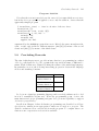
Syntax
When presenting pure Prolog programs we adhere to the usual syntactic conventions of Prolog. So each query and clause ends with the period “.” and in the unit
clauses “ ← ” is omitted. Unit clauses are called facts and non-unit clauses are
called rules. Of course, queries and clauses can be broken over several lines. To
maintain the spirit of logic programming, when presenting the programs, instead
of Prolog’s “:-” we use here the logic programming “ ← ”.
By a definition of a relation symbol p in a given program P we mean the set of
all clauses of P which use p in their heads. In Prolog terminology relation symbol
is synonymous with predicate.
Strings starting with a lower-case letter are reserved for the names of function or
relation symbols. For example f stands for a constant, function or relation symbol.
Additionally, we use here integers as constants. In turn, each string starting with
a capital letter or “ ” (underscore) is identified with a variable. For example Xs is
a variable. Comment lines start by the “%” symbol.
There are, however two important differences between the syntax of logic programming and of Prolog which need to be mentioned here.
Ambivalent Syntax
In first-order logic and, consequently, in logic programming, it is assumed that
function and relation symbols of different arity form mutually disjoint classes of
symbols. While this assumption is rarely stated explicitly, it is a folklore postulate
in mathematical logic which can be easily tested by exposing a logician to Prolog
syntax and wait for his protests. Namely, in contrast to first-order logic, in Prolog
the same name can be used for function or relation symbols of different arity.
Moreover, the same name with the same arity can be used for function and relation
symbols. This facility is called ambivalent syntax .
A function or a relation symbol f of arity n is then referred to as f/n. So in a
Prolog program we can use both a relation symbol p/2 and function symbols p/1
and p/2 and build syntactically legal facts like p(p(a,b), [c,p(a)]).
In the presence of ambivalent syntax the distinction between function symbols
and relation symbols and, consequently, between terms and atoms, disappears
but in the context of queries and clauses it is clear which symbol refers to which
syntactic category. The ambivalent syntax facility allows us to use the same name
for naturally related function or relation symbols.
In the presence of the ambivalent syntax we need to modify the Martelli–Monta-
106 Programming in Pure Prolog
nari algorithm given in Section 2.6 by allowing in action (2) the possibility that
the function symbols are equal. The appropriate modification is the following one:
(2′ ) f (s1 , ..., sn ) = g(t1 , ..., tm ) where f 6= g or n 6= m
halt with failure.
Throughout this chapter we refer to nullary function symbols as constants, and
to function symbols of positive arity as function symbols.
Anonymous Variables
Prolog allows so-called anonymous variables, written as “ ” (underscore). These
variables have a special interpretation, because each occurrence of “ ” in a query or
in a clause is interpreted as a different variable. Thus by definition each anonymous
variable occurs in a query or a clause only once.
At this stage it is too early to discuss the advantages of the use of anonymous
variables. We shall return to their use within the context of specific programs.
Anonymous variables form a simple and elegant device which sometimes increases
the readability of programs in a remarkable way.
Modern versions of Prolog, like SICStus Prolog [CW93], encourage the use of
anonymous variables by issuing a warning if a non-anonymous variable that occurs
only once in a clause is encountered.
We incorporate both of these syntactic facilities into pure Prolog.
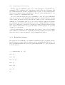
5.1.2
Computing
We now explain the computation process used in Prolog. First of all, the leftmost
selection rule is used. To simplify the subsequent discussion we now introduce the
following terminology. By an LD-resolvent we mean an SLD-resolvent w.r.t. the
leftmost selection rule and by an LD-tree an SLD-tree w.r.t. the leftmost selection
rule. The notions of LD-resolution and LD-derivation have the expected meaning.
Next, the clauses are tried in the order in which they appear in the program text.
So the program is viewed as a sequence and not as a set of clauses. In addition, for
the efficiency reasons, the occur-check is omitted from the unification algorithm.
We adopt these choices in pure Prolog.
The Strong Completeness of SLD-resolution (Theorem 4.13) tells us that (up
to renaming) all computed answers to a given query can be found in any SLDtree. However, without imposing any further restrictions on the SLD-resolution,
the computation process of logic programming, the resulting programs can become
hopelessly inefficient even if we restrict our attention to the leftmost selection rule.
In other words, the way the answers to the query are searched for becomes crucial
from the efficiency point of view.
If we traverse an LD-tree by means of breadth-first search, that is level by level,
it is guaranteed that an answer will be found, if there is any, but this search process
Introduction
107
can take exponential time in the depth of the tree and also requires exponential
space in the depth of the tree to store all the visited nodes. If we traverse this tree
by means of a depth-first search (to be explained more precisely in a moment),
that is informally, by pursuing the search first down each branch, often the answer
can be found in linear time in the depth of the tree but a divergence may result in
the presence of an infinite branch.
In Prolog the latter alternative, that is the depth-first search, is taken. Let us
explain now this search process in more detail.
Depth-first Search
By an ordered tree we mean here a tree in which the direct descendants of every
node are totally ordered.
The depth-first search is a search through a finitely branching ordered tree, the
main characteristic of which is that for each node all of its descendants are visited
before its siblings lying to its right. In this search no edge of the tree is traversed
more than once.
Depth-first search can be described as follows. Consider a finitely branching
ordered tree all the leaves of which are marked by a success or a fail marker.
The search starts at the root of the tree and proceeds by descending to its first
descendant. This process continues as long as a node has some descendants (so it
is not a leaf).
If a leaf marked success is encountered, then this fact is reported. If a leaf marked
fail is encountered, then backtracking takes place, that is the search proceeds by
moving back to the parent node of the leaf whereupon the next descendant of this
parent node is selected. This process continues until control is back at the root
node and all of its descendants have been visited. If the depth-first search enters
an infinite path before visiting a node marked success, then a divergence results.
In the case of Prolog the depth-first search takes place on an LD-tree for the
query and program under consideration. If a leaf marked success (that is the node
with the empty query) is encountered, then the associated c.a.s. is printed and the
search is suspended. The request for more solutions (“;”) results in a resumption
of the search from the last node marked success until a new noded marked success
is visited. If the tree has no (more) nodes marked success, then failure is reported,
by printing the answer “no”.
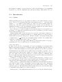
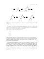
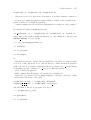
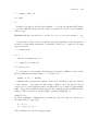
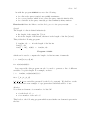
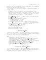
For the LD-tree given in Figure 3.1 the depth-first search is depicted in Figure
5.1.
The above description of the depth-first search is still somewhat informal, so we
provide an alternative description of it which takes into account that in an LD-tree
the nodes lying to the right of an infinite branch will not be visited. To this end we
define the subtree of the LD-tree which consists of the nodes that will be generated
during the depth-first search. As the order of the program clauses is now taken
into account this tree will be ordered.
108 Programming in Pure Prolog
success
fail
success
Figure 5.1 Backtracking over the LD-tree of Figure 3.1
Definition 5.1 For a given program we build a finitely branching ordered tree of
queries, possibly marked with the markers success and fail , by starting with the
initial query and repeatedly applying to it an operator expand(T , Q) where T is
the current tree and Q is the leftmost unmarked query.
expand(T , Q) is defined as follows.
• success: Q is the empty query;
mark Q with success,
• fail: Q has no LD-resolvents;
mark Q with fail,
• expand: Q has LD-resolvents;
let k be the number of clauses of the program that are applicable to the
selected atom. Add to T as direct descendants of Q k LD-resolvents of Q,
each with a different program clause. Choose these resolvents in such a way
that the paths of the tree remain initial fragments of LD-derivations. Order
them according to the order the applicable clauses appear in the program.
The limit of this process is an ordered tree of (possibly marked) queries. We call
this tree a Prolog tree.
2
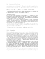
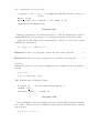
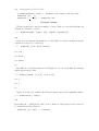
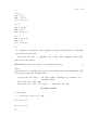
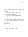
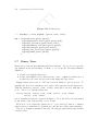
Example 5.2
(i) Consider the following program P1 :
p ← q.
p.
q ← r.
q ← s.
Introduction
109
p
p
exp.
p
exp.
exp.
q
q
r
p
r
fail
p
exp.
q
s
s
q
r
s
fail fail
p
exp.
q
success
r
s
fail fail
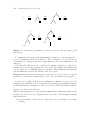
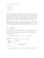
Figure 5.2 Step-by-step construction of the Prolog tree for the program P1 and
the query p
In Figure 5.2 we show a step-by-step construction of the Prolog tree for the
query p. Note that this tree is finite and the empty query is eventually marked
with success. In other words this tree is successful.
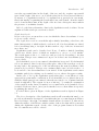
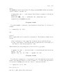
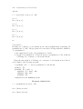
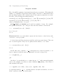
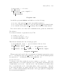
(ii) Consider now the following program P2 :
p ←
p.
q ←
q ←
s ←
q.
r.
s.
s.
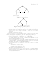
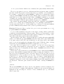
The last clause forms the only difference with the previous program. In Figure 5.3
we depict a step-by-step construction of the Prolog tree for the query p. Note that
this tree is infinite and the empty query is never visited. In this case the Prolog
tree is infinite and unsuccessful.
2
The step-by-step construction of the Prolog tree generates a sequence of consecutively selected nodes; in Figure 5.2 these are the following five queries: p,
q, r, s and 2. These nodes correspond to the nodes successively visited during the depth-first search over the corresponding LD-tree with the only difference
that the backtracking to the parent node has become “invisible”. Finally, note
that the unmarked leaves of a Prolog tree are never visited during the depth-first
search. Consequently, their descendants are not even generated during the depthfirst search.
110 Programming in Pure Prolog
p
p
p
exp.
exp.
exp.
q
q
r
s
p
p
q
r
fail
q
exp.
exp.
...
s
r
fail
s
s
Figure 5.3 Step-by-step construction of the Prolog tree for the program P2 and
the query p
To summarize, the basic search mechanism for answers to a query in pure Prolog is a depth-first search in an LD-tree. The construction of a Prolog tree is
an abstraction of this process but it approximates it in a way sufficient for our
purposes.
Note that the LD-trees can be obtained by a simple modification of the above
expansion process by disregarding the order of the descendants and applying the
expand operator to all unmarked queries each time. This summarizes in a succinct
way the difference between the LD-trees and Prolog trees.
Exercise 48 Characterize the situations in which the Prolog tree and the corresponding LD-tree coincide if the markers and the order of the descendants are disregarded.
2
So pure Prolog differs from logic programming in a number of aspects. Consequently, after explaining how to program in the resulting programming language
we shall discuss the consequences of the above choices in the subsequent chapters.
Outcomes of Prolog Computations
When considering pure Prolog programs it is important to understand what are the
possible outcomes of Prolog computations. For the sake of this discussion assume
that in LD-trees:
• the descendants of each node are ordered in a way conforming to the clause
ordering,
Introduction
success
success
111
fail
...
(infinite branch)
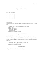
Figure 5.4 A query diverges
fail
success
...
(infinite branch)
Figure 5.5 A query potentially diverges
• the input clauses are obtained in a fixed way (for example, as already suggested in Section 3.2, by adding a subscript “i ” at the level i to all clause
variables),
• the mgus are chosen in a fixed way.
Then for every query Q and a program P exactly one LD-tree for P ∪{Q} exists.
Given a query Q and a program P , we introduce the following terminology.
• Q universally terminates if the LD-tree for P ∪ {Q} is finite.
For example the query p(X,c) for the program PATH of Example 3.36 universally terminates as Figure 3.1 shows.
• Q diverges if in the LD-tree for P ∪ {Q} an infinite branch exists to the left
of any success node. In particular, Q diverges if the LD-tree is not successful
and infinite. This situation is represented in Figure 5.4.
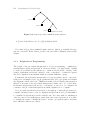
• Q potentially diverges if in the LD-tree for P ∪ {Q} a success node exists
such that
– all branches to its left are finite,
– an infinite branch exists to its right.
This situation is represented in Figure 5.5.
• Q produces infinitely many answers if the LD-tree for P ∪ {Q} has infinitely
many success nodes and all infinite branches lie to the right of them; Figure
5.6 represents this situation.
112 Programming in Pure Prolog
success
success
...
success (infinite branch)
Figure 5.6 A query produces infinitely many answers
• Q fails if the LD-tree for P ∪ {Q} is finitely failed.
Note that if Q produces infinitely many answers, then it potentially diverges,
but not conversely. Each of these possible outcomes will be illustrated later in the
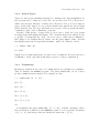
chapter.
5.1.3
Pragmatics of Programming
The details of the procedural interpretation of logic programming — unification,
standardization apart and generation of new resolvents — are quite subtle. Adding
to it the above mentioned modifications — leftmost selection rule, ordering of the
clauses, depth-first search and omission of the occur-check — results in a pretty
involved computation mechanism which is certainly difficult to grasp.
Fortunately, the declarative interpretation of logic programs comes to our rescue.
Using it we can simply view logic programs and pure Prolog programs as formulas
in a fragment of first-order logic. Thinking in terms of the declarative interpretation
instead of in terms of the procedural interpretation turns out to be of great help.
Declarative interpretation allows us to concentrate on what is to be computed, in
contrast to the procedural interpretation which explains how to compute.
Now, program specification is precisely a description of what the program is to
compute. In many cases to solve a computational problem in Prolog it just suffices
to formalize its specification in the clausal form. Of course such a formalization
often becomes a very inefficient program. But after some experience it is possible
to identify the causes of inefficiency and to learn to program in such a way that
more efficient solutions are offered.
Introduction
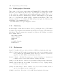
5.1.4
113
Interaction with a Prolog System
Here is the shortest possible description of how a Prolog system can be used. For
a more complete description the reader is referred to a language manual. The
interaction starts by typing cprolog for C-Prolog or sicstus for SICStus Prolog.
There are some small differences in interaction with these two systems which we
shall disregard. The system replies by the prompt “| ?-”. Now the program can
be read in by typing [file-name] followed by the period “.”. Assuming that the
program is syntactically correct, the system replies with the answer “yes” followed
by the prompt “| ?-”. Now a query to the program can be submitted, by typing
it with the period “.” at its end. The system replies are of two forms. If the
query succeeds, the corresponding computed answer substitution is printed in an
equational form; “yes” is used to denote the empty substitution.
At this point typing the return key terminates the computation, whereas typing
“;” followed by the return key is interpreted as the request to produce the next
computed answer substitution. If the query or the request to produce the next
answer (finitely) fails, “no” is printed. Below, we use queries both to find one
answer (the first one found by the depth-first search procedure) and to find all
answers. Finally, typing halt. finishes the interaction with the system.
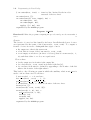
Here is an example of an interaction with C-Prolog:
cprolog
C-Prolog version 1.5
| ?- [test].
% read in the file called test;
test consulted 5112 bytes 0.15 sec.
yes
% the file read in;
| ?- app([a,b], [c,d], Zs). % compute an answer to the query
% app([a,b], [c,d], Zs);
Zs = [a,b,c,d]
% an answer is produced;
yes
| ?- sum(0, s(0), Z).
Z = s(0) ;
%
%
%
%
an answer to typing the return key;
compute an answer to the query
sum(0, s(0), Z);
‘‘;’’ is a request for more solutions;
no
| ?- halt.
% no more solutions;
% leave the system.
[ Prolog execution halted ]
Below, when listing the interactions with the Prolog system, the queries are written with the prompt string “| ?-” preceding them and the period “.” succeeding
them.
114 Programming in Pure Prolog
5.2
The Empty Domain
We found it convenient to organize the exposition in terms of domains over which
computing takes place. The simplest possible domain is the empty domain. Not
much can be computed over it. Still, for pure academic interest, legal Prolog
programs which compute over this domain can be written. An example is the
program considered in Chapter 3, now written conforming to the above syntax
conventions:
summer.
warm ← summer.
warm ← sunny.
happy ← summer, warm.
Program: SUMMER
We can query this program to obtain answers to simple questions. In absence of
variables all computed answer substitutions are empty. For example, we have
| ?- happy.
yes
| ?- sunny.
no
Exercise 49 Draw the Prolog trees for these two queries.
2
Prolog provides three built-in nullary relation symbols — true/0, fail/0 and
repeat/0. true/0 is defined internally by the single clause:
true.
so the query true always succeeds. fail/0 has the empty definition, so the query
fail always fails. Finally, repeat/0 is internally defined by the following clauses:
repeat.
repeat ← repeat.
The qualification “built-in” means that these relations cannot be redefined, so
clauses, the heads of which refer to the built-in relations, are ignored. In more
modern versions of Prolog, like SICStus Prolog, a warning is issued in case such
an attempt at redefining a built-in relation is encountered.
Exercise 50
(i) Draw the LD-tree and the Prolog tree for the query repeat, fail.
(ii) The command write(’a’) of Prolog prints the string a on the screen and the command nl produces a new line. What is the effect of the query repeat, write(’a’),
nl, fail? Does this query diverge or potentially diverge?
2
Finite Domains
5.3
115
Finite Domains
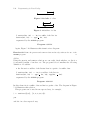
Slightly less trivial domains are the finite ones. With each element in the domain there corresponds a constant in the language; no other function symbols are
available.
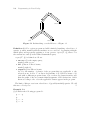
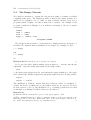
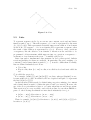
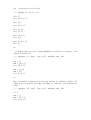
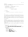
Even such limited domains can be useful. Consider for example a simple database
providing an information which countries are neighbours. To save toner let us
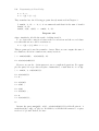
consider Central America (see Figure 5.7).
Belize
Guatemala
Honduras
El Salvador
Nicaragua
Costa Rica
Panama
Figure 5.7 Map of Central America
% neighbour(X, Y) ← X is a neighbour of Y.
neighbour(belize, guatemala).
neighbour(guatemala, belize).
neighbour(guatemala, el salvador).
neighbour(guatemala, honduras).
neighbour(el salvador, guatemala).
neighbour(el salvador, honduras).
neighbour(honduras, guatemala).
neighbour(honduras, el salvador).
neighbour(honduras, nicaragua).
neighbour(nicaragua, honduras).
neighbour(nicaragua, costa rica).
neighbour(costa rica, nicaragua).
neighbour(costa rica, panama).
neighbour(panama, costa rica).
Program: CENTRAL AMERICA
116 Programming in Pure Prolog
Here and elsewhere we precede the definition of each relation symbol by a comment line explaining its intended meaning.
We can now ask various simple questions, like
“are Honduras and El Salvador neighbours?”
| ?- neighbour(honduras, el_salvador).
yes
“which countries are neighbours of Nicaragua?”
| ?-
neighbour(nicaragua, X).
X = honduras ;
X = costa_rica ;
no
“which countries have both Honduras and Costa Rica as a neighbour?”
| ?- neighbour(X, honduras), neighbour(X, costa_rica).
X = nicaragua ;
no
The query neighbour(X, Y) lists all pairs of countries in the database (we omit
the listing) and, not unexpectedly, we have
| ?- neighbour(X, X).
no
Exercise 51 Formulate a query that computes all the triplets of countries which are
neighbours of each other.
2
Exercise 52
(i) Define a relation diff such that diff(X, Y) iff X and Y are different countries. How
many clauses are needed to define diff?
(ii) Formulate a query that computes all the pairs of countries that have Guatemala as
a neighbour.
2
Exercise 53 Consider the following question:
“are there triplets of countries which are neighbours of each other?”
and the following formalization of it as a query:
Finite Domains
117
neighbour(X, Y), neighbour(Y, Z), neighbour(X, Z).
Why is it not needed to state in the query that X, Y and Z are different countries? 2
Some more complicated queries require addition of rules to the considered program. Consider for example the question
“which countries can one reach from Guatemala by crossing one other country?”
It is answered by first formulating the rule
one crossing(X, Y) ← neighbour(X, Z), neighbour(Z, Y), diff(X, Y).
where diff is the relation defined in Exercise 52, and adding it to the program
CENTRAL AMERICA. Now we obtain
| ?- one_crossing(guatemala, Y).
Y = honduras ;
Y = el_salvador ;
Y = nicaragua ;
no
This rule allowed us to “mask” the local variable Z. A variable of a clause is called
local if it occurs only in its body. One should not confuse anonymous variables
with local ones. For example, replacing in the above clause Z by “ ” would change
its meaning, as each occurrence of “ ” denotes a different variable.
Next, consider the question
“which countries have Honduras or Costa Rica as a neighbour?”
In pure Prolog, clause bodies are simply sequences of atoms, so we need to define
a new relation by means of two rules:
neighbour h or c(X) ← neighbour(X, honduras).
neighbour h or c(X) ← neighbour(X, costa rica).
and add them to the above program. Now we get
| ?- neighbour_h_or_c(X).
X = guatemala ;
X = el_salvador ;
118 Programming in Pure Prolog
X = nicaragua ;
X = nicaragua ;
X = panama ;
no
The answer nicaragua is listed twice due to the fact that it is a neighbour of
both countries. The above representation of the neighbour relation is very simple
minded and consequently various natural questions, like “which country has the
largest number of neighbours?” or “which countries does one need to cross when
going from country X to country Y?” cannot be easily answered. A more appropriate
representation is where for each country an explicit list of its neighbours is made.
We shall return to this issue after we have introduced the concept of lists.
Exercise 54 Assume the unary relations female and male and the binary relations
mother and father. Write a pure Prolog program that defines the binary relations son,
daughter, parent, grandmother, grandfather and grandparent. Set up a small
database of some family and run some example queries that involve the new relations.
2
5.4
Numerals
Natural numbers can be represented in many ways. Perhaps the most simple
representation is by means of a constant 0 (zero), and a unary function symbol s
(successor). We call the resulting ground terms numerals. Formally, numerals are
defined inductively as follows:
• 0 is a numeral,
• if x is a numeral, then s(x), the successor of x, is a numeral.
Numeral
This definition directly translates into the following program:
% num(X) ← X is a numeral.
num(0).
num(s(X)) ← num(X).
Program: NUMERAL
It is easy to see that
• for a numeral sn (0), where n ≥ 0, the query num(sn (0)) successfully terminates,
Numerals
119
• for a ground term t which is not a numeral, the query num(t) finitely fails.
The above program is recursive, which means that its relation, num, is defined
in terms of itself. In general, recursion introduces a possibility of non-termination.
For example, consider the program NUMERAL1 obtained by reordering the clauses
of the program NUMERAL and take the query num(Y) with a variable Y. As Y unifies
with s(X), we see that, using the first clause of NUMERAL1, num(X) is a resolvent
of num(Y). By repeating this procedure we obtain an infinite computation which
starts with num(Y). Thus the query num(Y) diverges w.r.t. NUMERAL1.
In contrast, the query num(Y), when used with the original program NUMERAL,
yields a c.a.s. {Y/0}. Upon backtracking the c.a.s.s {Y/s(0)}, {Y/s(s(0))}, . . .
are successively produced. So, in the terminology of Section 5.1, the query num(Y)
produces infinitely many answers and a fortiori potentially diverges.
Exercise 55 Draw the LD-tree and the Prolog tree for the query num(Y) w.r.t. to the
programs NUMERAL and NUMERAL1.
2
So we see that termination depends on the clause ordering, which considerably
complicates an understanding of the programs. Therefore it is preferable to write
the programs in such a way that the desired queries terminate for all clause orderings, that is that these queries universally terminate.
Another aspect of the clause ordering is efficiency. Consider the query num(sn (0))
with n > 0. With the program NUMERAL1 the first clause will be successfully used
for n times, then it will “fail” upon which the second clause will be successfully
used. So in total n+2 unification attempts will be made. With the clause ordering
used in the program NUMERAL this number equals 2n+1, so is ≥ n+2.
Of course, the above query is not a “typical” one but one can at least draw
the conclusion that usually in a term there are more occurrences of the function
symbol s than of 0. Consequently, the first clause of NUMERAL succeeds less often
than the second one.
This seems to suggest that the program NUMERAL1 is more efficient than NUMERAL.
However, this discussion assumes that the clauses forming the definition of a relation are tried sequentially in the order they appear in the program. In most
implementations of Prolog this is not the case. Namely an indexing mechanism
is used (see e.g. Aı̈t-Kaci [Ait91, pages 65–72]), according to which initially the
first argument of the selected atom with a relation p is compared with the first
argument of the head of each of the clauses defining p and all incompatible clauses
are discarded. Then the gain obtained from the clause ordering in NUMERAL1 is
lost.
Addition
The program NUMERAL can only be used to test whether a term is a numeral. Let
us see now how to compute with numerals. Addition is an operation defined on
numerals by the following two axioms of Peano arithmetic (see e.g. Shoenfield
[Sho67, page 22]):
120 Programming in Pure Prolog
• x + 0 = x,
• x + s(y) = s(x + y).
They translate into the following program already mentioned in Chapter 3:
% sum(X, Y, Z) ← X, Y, Z are numerals such that Z is the sum of X and Y.
sum(X, 0, X).
sum(X, s(Y), s(Z)) ← sum(X, Y, Z).
Program: SUM
where, intuitively, Z holds the result of adding X and Y.
To see better the connection between the second axiom and the second clause
note that this axiom could be rewritten as
• x + s(y) = s(z), where z = x + y.
This program can be used in a number of ways. First, we can compute the sum of
two numbers, albeit in a cumbersome, unary notation:
| ?- sum(s(s(0)),
s(s(s(0))), Z).
Z = s(s(s(s(s(0)))))
However, we can also obtain answers to more complicated questions. For example, the query below produces all pairs of numerals X, Y such that X + Y = s3 (0):
| ?- sum(X, Y, s(s(s(0)))).
X = s(s(s(0)))
Y = 0 ;
X = s(s(0))
Y = s(0) ;
X = s(0)
Y = s(s(0)) ;
X = 0
Y = s(s(s(0))) ;
no
In turn, the query sum(s(X), s(Y), s(s(s(s(s(0)))))) yields all pairs X, Y
such that s(X) + s(Y) = s5 (0), etc. In addition, recall that the answers to a query
need not be ground. Indeed, we have
Numerals
121
| ?- sum(X, s(0), Z).
Z = s(X) ;
no
Finally, some queries, like the query sum(X, Y, Z) already discussed in Chapter
3, produce infinitely many answers. Other programs below can be used in similar,
diverse ways.
Exercise 56 Draw the the LD-tree and the Prolog tree for the query sum(X, Y, Z).
2
Notice that we did not enforce anywhere that the arguments of the sum relation
should be terms which instantiate to numerals. Indeed, we obtain the following
expected answer
| ?- sum(a,0,X).
X = a
. . . but also an unexpected one:
| ?- sum([a,b,c],s(0),X).
X = s([a,b,c])
To safeguard oneself against such unexpected (ab)uses of SUM we need to insert
the test num(X) in the first clause, i.e. to change it to
sum(X, 0, X) ← num(X).
Omitting this test puts the burden on the user; including it puts the burden
on the system — each time the first clause of SUM is used, the inserted test is
carried out. Note that with the sum so modified the above considered query sum(X,
s(0), Z) produces infinitely many answers, since num(X) produces infinitely many
answers. These answers are {X/0, Z/s(0)}, {X/s(0), Z/s(s(0))}, etc.
Multiplication
In Peano arithmetic, multiplication is defined by the following two axioms (see
Shoenfield [Sho67, page 22]):
• x · 0 = 0,
• x · s(y) = (x · y) + x.
They translate into the following program:
122 Programming in Pure Prolog
% mult(X, Y, Z) ← X, Y, Z are numerals such that Z is the product of X
and Y.
mult( , 0, 0).
mult(X, s(Y), Z) ← mult(X, Y, W), sum(W, X, Z).
augmented by the SUM program.
Program: MULT
In this program the local variable W is used to hold the intermediate result of
multiplying X and Y. Note the use of an anonymous variable in the first clause.
Again, the second clause can be better understood if the second axiom for multiplication is rewritten as
• x · s(y) = w + x, where w = x · y.
Exercise 57 Write a program that computes the sum of three numerals.
2
Exercise 58 Write a program computing the exponent XY of two numerals.
2
Less than
Finally, the relation < (less than) on numerals can be defined by the following two
axioms:
• 0 < s(x),
• if x < y, then s(x) < s(y).
They translate into following program:
% less(X, Y) ← X, Y are numerals such that X < Y.
less(0, s( )).
less(s(X), s(Y)) ← less(X, Y).
Program: LESS
It is worthwhile to note here that the above two axioms differ from the formalization of the < relation in Peano arithmetic, where among others the linear ordering
axiom is used:
• x < y ∨ x = y ∨ y < x.
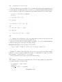
Lists
[.|.]
a





BB
BB
BB
BB
[.|.]
b
123
||
||
|
|
||
BB
BB
BB
BB
[.|.]
c
||
||
|
|
||
AA
AA
AA
A
[ ]
Figure 5.8 A list
5.5
Lists
To represent sequences in Prolog we can use any constant, say 0 and any binary
function symbol, say f . Then the sequence a, b, c can be represented by the term
f (a, f (b, f (c, 0))). This representation trivially supports an addition of an element
at the front of a sequence — if e is an element and s represents a sequence, then
the result of this addition is represented by f (e, s). However, other operations
on sequences, like the deletion of an element or insertion at the end have to be
programmed. A data structure which supports just one operation on sequences —
an insertion of an element at the front — is usually called a list.
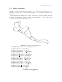
Lists form such a fundamental data structure in Prolog that special, built-in
notational facilities for them are available. In particular, the pair consisting of a
constant [] and a binary function symbol [.|..] is used to define them. Formally,
lists are defined inductively as follows:
• [] is a list,
• if xs is a list, then [x | xs] is a list; x is called its head and xs is called its
tail .
[] is called the empty list.
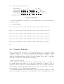
For example, [s(0)|[]] and [0|[X|[]]] are lists, whereas [0|s(0)] is not,
because s(0) is not a list. In addition, the tree depicted in Figure 5.8 represents
the list [a|[b|[c|[]]]].
As already stated, lists can also be defined using any pair consisting of a constant
and a binary function symbol. (Often the pair nil and cons is used.) However, the
use of the above pair makes it easier to recognize when lists are used in programs.
This notation is not very readable, and even short lists become then difficult to
parse. So the following shorthands are introduced inductively for n ≥ 1:
• [s0 |[s1 , ..., sn |t]] abbreviates to [s0 , s1 , ..., sn |t],
• [s0 , s1 , ..., sn |[ ]] abbreviates to [s0 , s1 , ..., sn ].
Thus for example, [a|[b|c]] abbreviates to [a,b|c], and [a|[b,c|[]]] abbreviates to [a,b,c].
124 Programming in Pure Prolog
The following interaction with a Prolog system shows that these simplifications
are also carried out internally. Here =/2 is Prolog’s built-in written using the infix
notation (that is, between the arguments) and defined internally by a single clause:
% X = Y ← X and Y are unifiable.
X = X.
| ?- X = [a | [b | c]].
X = [a,b|c]
| ?- [a,b|c]
= [a | [b | c]].
yes
| ?- X = [a | [b, c | []]].
X = [a,b,c]
| ?- [a,b,c] = [a | [b, c | []]].
yes
To enhance the readability of the programs that use lists we incorporate the
above notation and abbreviations into pure Prolog.
The above abbreviations easily confuse a beginner. To test your understanding
of this notation please solve the following exercise.
Exercise 59 Which of the following terms are lists:
[a,b], [a|b], [a|[b|c]], [a,[b,c]], [a,[b|c]], [a|[b,c]]?
2
Further, to enhance the readability, we also use in programs the names ending
with “s” to denote variables which are meant to be instantiated to lists. Note that
the elements of a list need not to be ground.
We now present a pot-pourri of programs that use lists.
List
The definition of lists directly translates into the following simple program which
recognizes whether a term is a list:
% list(Xs) ← Xs is a list.
list([]).
list([ | Ts]) ← list(Ts).
Program: LIST
Lists
125
As with the program NUMERAL we note the following:
• for a list t the query list(t) successfully terminates,
• for a ground term t which is not a list, the query list(t) finitely fails,
• for a variable X, the query list(X) produces infinitely many answers.
Exercise 60 Draw the LD-tree and the Prolog tree for the query list(X).
2
Length
The length of a list is defined inductively:
• the length of the empty list [] is 0,
• if n is the length of the list xs, then n+1 is the length of the list [x|xs].
This yields the following program:
% len(Xs, X) ← X is the length of the list Xs.
len([], 0).
len([ | Ts], s(N)) ← len(Ts, N).
Program: LENGTH
which can be used to compute the length of a list in terms of numerals:
| ?- len([a,b,a,d],N).
N = s(s(s(s(0))))
Less expectedly, this program can also be used to generate a list of different
variables of a given length. For example, we have:
| ?-
len(Xs, s(s(s(s(0)))) ).
Xs = [_A,_B,_C,_D]
( A, B, C, D are variables generated by the Prolog system). We shall see at the
end of this section an example of a program where such lists will be of use.
Member
Note that an element x is a member of a list l iff
• x is the head of l or
• x is a member of the tail of l.
This leads to the following program which tests whether an element is present in
the list:
126 Programming in Pure Prolog
% member(Element, List) ← Element is an element of the list List.
member(X, [X | ]).
member(X, [ | Xs]) ← member(X, Xs).
Program: MEMBER
This program can be used in a number of ways. First, we can check whether an
element is a member of a list:
| ?-
member(august, [june, july, august, september]).
yes
Next, we can generate all members of a list (this is a classic example from the
original C-Prolog User’s Manual ):
| ?-
member(X, [tom, dick, harry]).
X = tom ;
X = dick ;
X = harry ;
no
In addition, as already mentioned in Chapter 1, we can easily find all elements
which appear in two lists:
| ?- member_both(X, [1,2,3], [2,3,4,5]).
X = 2 ;
X = 3 ;
no
Again, as in the case of SUM, some ill-typed queries may yield a puzzling answer:
| ?- member(0,[0 | s(0)]).
yes
Recall that [0 | s(0)] is not a list. A “no” answer to such a query can be enforced
by replacing the first clause by
member(X, [X | Xs]) ← list(Xs).
Lists
127
Subset
The MEMBER program is used in the following program SUBSET which tests whether
a list is a subset of another one:
% subset(Xs, Ys) ← each element of the list Xs is a member of the list Ys.
subset([], ).
subset([X | Xs], Ys) ← member(X, Ys), subset(Xs, Ys).
augmented by the MEMBER program.
Program: SUBSET
Note that multiple occurrences of an element are allowed here. So we have for
example
| ?- subset([a, a], [a]).
yes
Append
More complex lists can be formed by concatenation. The inductive definition is as
follows:
• the concatenation of the empty list [] and the list ys yields the list ys,
• if the concatenation of the lists xs and ys equals zs, the concatenation of
the lists [x | xs] and ys equals [x | zs].
This translates into the perhaps most often cited Prolog program:
% app(Xs, Ys, Zs) ← Zs is the result of concatenating the lists Xs and Ys.
app([], Ys, Ys).
app([X | Xs], Ys, [X | Zs]) ← app(Xs, Ys, Zs).
Program: APPEND
Note that the computation of concatenation of two lists takes linear time in the
length of the first list. Indeed, for a list of length n, n + 1 calls of the app relation
are generated. APPEND can be used not only to concatenate the lists:
| ?- app([a,b], [a,c], Zs).
Zs = [a,b,a,c]
but also to split a list in all possible ways:
128 Programming in Pure Prolog
| ?- app(Xs, Ys, [a,b,a,c]).
Xs = []
Ys = [a,b,a,c] ;
Xs = [a]
Ys = [b,a,c] ;
Xs = [a,b]
Ys = [a,c] ;
Xs = [a,b,a]
Ys = [c] ;
Xs = [a,b,a,c]
Ys = [] ;
no
Combining these two ways of using APPEND we can delete an occurrence of an
element from the list:
| ?- app(X1s, [a | X2s], [a,b,a,c]), app(X1s, X2s, Zs).
X1s = []
X2s = [b,a,c]
Zs = [b,a,c] ;
X1s = [a,b]
X2s = [c]
Zs = [a,b,c] ;
no
Here the result is computed in Zs and X1s and X2s are auxiliary variables. In
addition, we can generate all results of deleting an occurrence of an element from
a list:
| ?- app(X1s, [X | X2s], [a,b,a,c]), app(X1s, X2s, Zs).
X = a
X1s = []
X2s = [b,a,c]
Zs = [b,a,c] ;
Lists
129
X = b
X1s = [a]
X2s = [a,c]
Zs = [a,a,c] ;
X = a
X1s = [a,b]
X2s = [c]
Zs = [a,b,c] ;
X = c
X1s = [a,b,a]
X2s = []
Zs = [a,b,a] ;
no
To eliminate the printing of the auxiliary variables X1s and X2s we could define
a new relation by the rule
select(X, Xs, Zs) ← app(X1s, [X | X2s], Xs), app(X1s, X2s, Zs).
and use it in the queries.
Exercise 61 Write a program for concatenating three lists.
2
Select
Alternatively, we can define the deletion of an element from a list inductively. The
following program performs this task:
% select(X, Xs, Zs) ← Zs is the result of deleting one occurrence of X
from the list Xs.
select(X, [X | Xs], Xs).
select(X, [Y | Xs], [Y | Zs]) ← select(X, Xs, Zs).
Program: SELECT
Now we have
| ?- select(a, [a,b,a,c], Zs).
Zs = [b,a,c] ;
Zs = [a,b,c] ;
no
130 Programming in Pure Prolog
and also
| ?- select(X, [a,b,a,c], Zs).
X = a
Zs = [b,a,c] ;
X = b
Zs = [a,a,c] ;
X = a
Zs = [a,b,c] ;
X = c
Zs = [a,b,a] ;
no
Permutation
Deleting an occurrence of an element from a list is helpful when generating all
permutations of a list. The program below uses the following inductive definition
of a permutation:
• the empty list [] is the only permutation of itself,
• [x|ys] is a permutation of a list xs if ys is a permutation of the result zs
of deleting one occurrence of x from the list xs.
Using the first method of deleting one occurrence of an element from a list we
are brought to the following program:
% perm(Xs, Ys) ← Ys is a permutation of the list Xs.
perm([], []).
perm(Xs, [X | Ys]) ←
app(X1s, [X | X2s], Xs),
app(X1s, X2s, Zs),
perm(Zs, Ys).
augmented by the APPEND program.
Program: PERMUTATION
| ?- perm([here,we,are], Ys).
Ys = [here,we,are] ;
Ys = [here,are,we] ;
Lists
131
Ys
Xs
Figure 5.9 Prefix of a list
Ys = [we,here,are] ;
Ys = [we,are,here] ;
Ys = [are,here,we] ;
Ys = [are,we,here] ;
no
Permutation1
An alternative version uses the SELECT program to remove an element from the
list:
% perm(Xs, Ys) ← Ys is a permutation of the list Xs.
perm([], []).
perm(Xs, [X | Ys]) ←
select(X, Xs, Zs),
perm(Zs, Ys).
augmented by the SELECT program.
Program: PERMUTATION1
Prefix and Suffix
The APPEND program can also be elegantly used to formalize various sublist operations. An initial segment of a list is called a prefix and its final segment is called
a suffix . Using the APPEND program both relations can be defined in a straightforward way:
% prefix(Xs, Ys) ← Xs is a prefix of the list Ys.
prefix(Xs, Ys) ← app(Xs, , Ys).
augmented by the APPEND program.
Program: PREFIX
Figure 5.9 illustrates this situation in a diagram.
132 Programming in Pure Prolog
Xs
Ys
Figure 5.10 Suffix of a list
Xs
Zs
Ys
Figure 5.11 Sublist of a list
% suffix(Xs, Ys) ← Xs is a suffix of the list Ys.
suffix(Xs, Ys) ← app( , Xs, Ys).
augmented by the APPEND program.
Program: SUFFIX
Again, Figure 5.10 illustrates this situation in a diagram.
Exercise 62 Define the prefix and suffix relations directly, without the use of the
APPEND program.
2
Sublist
Using the prefix and suffix relations we can easily check whether one list is a
(consecutive) sublist of another one. The program below formalizes the following
definition of a sublist:
• the list as is a sublist of the list bs if as is a prefix of a suffix of bs.
% sublist(Xs, Ys) ← Xs is a sublist of the list Ys.
sublist(Xs, Ys) ← app( , Zs, Ys), app(Xs, , Zs).
augmented by the APPEND program.
Program: SUBLIST
In this clause Zs is a suffix of Ys and Xs is a prefix of Zs. The diagram in Figure
5.11 illustrates this relation.
This program can be used in an expected way, for example,
| ?- sublist([2,6], [5,2,3,2,6,4]).
yes
and also in a less expected way,
Lists
133
| ?- sublist([1,X,2], [4,Y,3,2]).
X = 3
Y = 1 ;
no
Here as an effect of the call of SUBLIST both lists become instantiated so that the
first one becomes a sublist of the second one. At the end of this section we shall
see a program where this type of instantiation is used in a powerful way to solve a
combinatorial problem.
Exercise 63 Write another version of the SUBLIST program which formalizes the following definition:
the list as is a sublist of the list bs if as is a suffix of a prefix of bs.
2
Naive Reverse
To reverse a list, the following program is often used:
% reverse(Xs, Ys) ← Ys is the result of reversing the list Xs.
reverse([], []).
reverse([X | Xs], Ys) ← reverse(Xs, Zs), app(Zs, [X], Ys).
augmented by the APPEND program.
Program: NAIVE REVERSE
This program is very inefficient and is often used as a benchmark program. It
leads to a number of computation steps, which is quadratic in the length of the
list. Indeed, translating the clauses into recurrence relations over the length of the
lists we obtain for the first clause:
r(x + 1) = r(x) + a(x),
a(x) = x + 1,
and for the second one:
r(0) = 1.
This yields r(x) = x · (x + 1)/2 + 1.
Reverse with Accumulator
A more efficient program is the following one:
% reverse(Xs, Ys) ← Ys is the reverse of the list Xs.
reverse(X1s, X2s) ← reverse(X1s, [], X2s).
% reverse(Xs, Ys, Zs) ← Zs is the result of concatenating
the reverse of the list Xs and the list Ys.
reverse([], Xs, Xs).
reverse([X | X1s], X2s, Ys) ← reverse(X1s, [X | X2s], Ys).
134 Programming in Pure Prolog
Program: REVERSE
Here, the middle argument of reverse/3 is used as an accumulator . This makes the
number of computation steps linear in the length of the list. To understand better
the way this program works consider its use for the query reverse([a,b,c],Ys).
It leads to the following successful derivation:
θ
θ
θ
1
2
3
reverse([a, b, c], Ys) =⇒
reverse([a, b, c], [ ], Ys) =⇒
reverse([b, c], [a], Ys) =⇒
1
3
3
θ
θ
4
5
reverse([c], [b, a], Ys) =⇒
reverse([ ], [c, b, a], Ys) =⇒
2,
3
2
where θ5 instantiates Ys to [c,b,a].
NAIVE REVERSE and REVERSE can be used in a number of ways. For example,
the query reverse(xs, [X | Ls]) produces the last element of the list xs:
| ?-
reverse([a,b,a,d], [X|Ls]).
Ls = [a,b,a]
X = d
Exercise 64 Write a program which computes the last element of a list directly, without the use of other programs.
2
So far we have used the anonymous variables only in program clauses. They can
also be used in queries. They are not printed in the answer, so we obtain
| ?- reverse([a,b,a,d], [X|_]).
X = d
Recall, that each occurrence of “ ” is interpreted as a different variable, so we
have (compare it with the query neighbour(X, X) used on page 116)
| ?- neighbour(_,_).
yes
One has to be careful and not to confuse the use of “ ” with existential quantification. For example, note that we cannot eliminate the printing of the values of
X1s and X2s in the query
| ?- app(X1s, [X | X2s], [a,b,a,c]), app(X1s, X2s, Zs).
by replacing them by “ ”, i.e. treating them as anonymous variables, as each of
them occurs more than once in the query.
Lists
135
Palindrome
Another use of the REVERSE program is present in the following program which
tests whether a list is a palindrome.
% palindrome(Xs) ← the list Xs is equal to its reverse.
palindrome(Xs) ← reverse(Xs, Xs).
augmented by the REVERSE program.
Program: PALINDROME
For example:
| ?-
palindrome(
[t,o,o,n, n,e,v,a,d,a, n,a, c,a,n,a,d,a, v,e,n,n,o,o,t]
).
yes
It is instructive to see for which programs introduced in this section it is possible to run successfully ill-typed queries, i.e. queries which do not have lists as
arguments in the places one would expect a list from the specification. These are
SUBSET, APPEND, SELECT and SUBLIST. For other programs the ill-typed queries
never succeed, essentially because the unit clauses can succeed only with properly
typed arguments.
A Sequence
The following delightful program (see Coelho and Cotta [CC88, page 193]) shows
how the use of anonymous variables can dramatically improve the program readability. Consider the following problem: arrange three 1s, three 2s, ..., three 9s in
sequence so that for all i ∈ [1, 9] there are exactly i numbers between successive
occurrences of i.
The desired program is an almost verbatim formalization of the problem in
Prolog.
% sequence(Xs) ← Xs is a list of 27 elements.
sequence([ , , , , , , , , , , , , , , , , , , , , , , , , , , ]).
% question(Ss) ← Ss is a list of 27 elements forming the desired sequence.
question(Ss) ←
sequence(Ss),
sublist([1, ,1, ,1], Ss),
sublist([2, , ,2, , ,2], Ss),
sublist([3, , , ,3, , , ,3], Ss),
sublist([4, , , , ,4, , , , ,4], Ss),
sublist([5, , , , , ,5, , , , , ,5], Ss),
136 Programming in Pure Prolog
sublist([6,
sublist([7,
sublist([8,
sublist([9,
,
,
,
,
,
,
,
,
,
,
,
,
,
,
,
,
,
,
,
,
,6, , , ,
, ,7, , ,
, , ,8, ,
, , , ,9,
,
,
,
,
,
,
,
,
,6], Ss),
, , ,7], Ss),
, , , , ,8], Ss),
, , , , , , ,9], Ss).
augmented by the SUBLIST program.
Program: SEQUENCE
The following interaction with Prolog shows that there are exactly six solutions
to this problem.
| ?- question(Ss).
Ss = [1,9,1,2,1,8,2,4,6,2,7,9,4,5,8,6,3,4,7,5,3,9,6,8,3,5,7] ;
Ss = [1,8,1,9,1,5,2,6,7,2,8,5,2,9,6,4,7,5,3,8,4,6,3,9,7,4,3] ;
Ss = [1,9,1,6,1,8,2,5,7,2,6,9,2,5,8,4,7,6,3,5,4,9,3,8,7,4,3] ;
Ss = [3,4,7,8,3,9,4,5,3,6,7,4,8,5,2,9,6,2,7,5,2,8,1,6,1,9,1] ;
Ss = [3,4,7,9,3,6,4,8,3,5,7,4,6,9,2,5,8,2,7,6,2,5,1,9,1,8,1] ;
Ss = [7,5,3,8,6,9,3,5,7,4,3,6,8,5,4,9,7,2,6,4,2,8,1,2,1,9,1] ;
no
5.6
Complex Domains
By a complex domain we mean here a domain built from some constants by means
of function symbols. Of course, both numerals and lists are examples of such
domains. In this section our interest lies in domains built by means of other,
application dependent, function symbols. Such domains correspond to compound
data types in imperative and functional languages.
A Map Colouring Program
As an example consider the problem of colouring a map in such a way that no
two neighbours have the same colour. Below we call such a colouring correct. A
solution to the problem can be greatly simplified by the use of an appropriate data
representation. The map is represented below as a list of regions and colours as a
list of available colours. This is hardly surprising.
The main insight lies in the representation of regions. In the program below each
region is determined by its name, colour and the colours of its neighbours, so it is
Complex Domains
137
represented as a term region(name, colour, neighbours), where neighbours
is a list of colours of the neighbouring regions.
The program below is a pretty close translation of the following definition of a
correct colouring:
• A map is correctly coloured iff each of its regions is correctly coloured.
• A region region(name,colour,neighbours) is correctly coloured, iff colour
and the elements of neighbours are members of the list of the available
colours and colour is not a member of the list neighbours.
% colour map(Map, Colours) ← Map is correctly coloured using Colours.
colour map([], ).
colour map([Region | Regions], Colours) ←
colour region(Region, Colours),
colour map(Regions, Colours).
% colour region(Region, Colours) ← Region and its neighbours are
correctly coloured using Colours.
colour region(region( , Colour, Neighbors), Colours) ←
select(Colour, Colours, Colours1),
subset(Neighbors, Colours1).
augmented by the SELECT program.
augmented by the SUBSET program.
Program: MAP COLOUR
Thus to use this program one first needs to represent the map in an appropriate way. Here is the appropriate representation for the map of Central America
expressed as a single atom with the relation symbol map:
map([
region(belize, Belize, [Guatemala]),
region(guatemala, Guatemala, [Belize, El Salvador, Honduras]),
region(el salvador, El Salvador, [Guatemala, Honduras]),
region(honduras, Honduras, [Guatemala, El Salvador, Nicaragua]),
region(nicaragua, Nicaragua, [Honduras, Costa rica]),
region(costa rica, Costa rica, [Nicaragua, Panama]),
region(panama, Panama, [Costa rica])
]).
Program: MAP OF CENTRAL AMERICA
Now, to link this representation with the MAP COLOUR program we just need to
use the following query which properly “initializes” the variable Map and where for
simplicity we already fixed the choice of available colours:
138 Programming in Pure Prolog
a
 ???

??

??


?

c
b>
>>
>>
>>
>
d
e
Figure 5.12 A binary tree
| ?- map(Map), colour_map(Map, [green, blue, red]).
Map = [region(belize,green,[blue]),
region(guatemala,blue,[green,green,red]),
region(el_salvador,green,[blue,red]),
region(honduras,red,[blue,green,green]),
region(nicaragua,green,[red,blue]),
region(costa_rica,blue,[green,green]),
region(panama,green,[blue])
]
5.7
Binary Trees
Binary trees form another fundamental data structure. Prolog does not provide
any built-in notational facilities for them, so we adopt the following inductive
definition:
• void is a (n empty) binary tree,
• if left and right are trees, then tree(x, left, right) is a binary tree; x
is called its root, left its left subtree and right its right subtree.
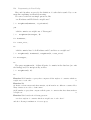
Empty binary trees serve to “fill” the nodes in which no data is stored. To
visualize the trees it is advantageous to ignore their presence in the binary tree.
Thus the binary tree tree(c, void, void) corresponds to the tree with just one
node — the root c, and the binary tree
tree(a, tree(b, tree(d, void, void), tree(e, void, void)),
tree(c, void, void))
can be visualized as the tree depicted in Figure 5.12. So the leaves are represented
by the terms of the form tree(s, void, void).
From now on we abbreviate binary tree to a tree and hope that no confusion
arises between a term that is a (binary) tree and the tree such a term visualizes.
The above definition translates into the following program which tests whether
a term is a tree.
Binary Trees
139
% bin tree(T) ← T is a tree.
bin tree(void).
bin tree(tree( , Left, Right)) ←
bin tree(Left),
bin tree(Right).
Program: TREE
As with the programs NUMERAL and LIST we note the following:
• for a tree t the query bin tree(t) successfully terminates,
• for a ground term t which is not a tree the query bin tree(t) finitely fails,
• for a variable X, the query bin tree(X) produces infinitely many answers.
Trees can be used to store data and to maintain various operations on this data.
Tree Member
Note that an element x is present in a tree T iff
• x is the root of T or
• x is in the left subtree of T or
• x is in the right subtree of T .
This directly translates into the following program:
% tree member(E, Tree)
tree member(X, tree(X,
tree member(X, tree( ,
tree member(X, tree( ,
← E is an element of the tree Tree.
, )).
Left, )) ← tree member(X, Left).
, Right)) ← tree member(X, Right).
Program: TREE MEMBER
This program can be used both to test whether an element x is present in a given
tree t — by using the query tree member(x, t), and to list all elements present
in a given tree t — by using the query tree member(X, t).
In-order Traversal
To traverse a tree three methods are most common: a pre-order — (in every
subtree) first the root is visited, then the nodes of left subtree and then the nodes
of right subtree; an in-order — first the nodes of the left subtree are visited, then
the root and then the nodes of the right subtree; and a post-order — first the
nodes of the left subtree are visited, then the nodes of the right subtree and then
the root. Each of them translates directly into a Prolog program. For example the
in-order traversal translates to
140 Programming in Pure Prolog
% in-order(Tree, List) ← List is a list obtained by the in-order
traversal of the tree Tree.
in-order(void, []).
in-order(tree(X, Left, Right), Xs) ←
in-order(Left, Ls),
in-order(Right, Rs),
app(Ls, [X | Rs], Xs).
augmented by the APPEND program.
Program: IN ORDER
Exercise 65 Write the programs computing the pre-order and post-order traversals of
a tree.
2
Frontier
The frontier of a tree is a list formed by its leaves. Recall that the leaves of a tree
are represented by the terms of the form tree(a, void, void). To compute a
frontier of a tree we need to distinguish three types of trees:
• the empty tree, that is the term void,
• a leaf, that is a term of the form tree(a, void, void),
• a non-empty, non-leaf tree (in short a nel-tree), that is a term tree(x, l,
r), such that either l or r does not equal void.
We now have:
• for the empty tree its frontier is the empty list,
• for a leaf tree(a, void, void) its frontier is the list [a],
• for a nel-tree its frontier is obtained by appending to the frontier of the left
subtree the frontier of the right subtree.
This leads to the following program in which the auxiliary relation nel tree is
used to enforce that a tree is a nel-tree:
% nel tree(t) ← t is a nel-tree.
nel tree(tree( , tree( , , ), )).
nel tree(tree( , , tree( , , ))).
% front(Tree, List) ← List is a frontier of the tree Tree.
front(void, []).
front(tree(X, void, void), [X]).
front(tree(X, L, R), Xs) ←
nel tree(tree(X, L, R)),
front(L, Ls),
front(R, Rs),
app(Ls, Rs, Xs).
augmented by the APPEND program.
Concluding Remarks
141
Program: FRONTIER
Note that the test nel tree(t) can also succeed for terms which are not trees,
but in the above program it is applied to trees only. In addition, observe that the
apparently simpler program
% front(Tree, List) ← List is a frontier of the tree Tree.
front(void, []).
front(tree(X, void, void), [X]).
front(tree( , L, R), Xs) ←
front(L, Ls),
front(R, Rs),
app(Ls, Rs, Xs).
augmented by the APPEND program is incorrect. Indeed, the query front(tree(X,
void, void), Xs) yields two different answers: {Xs/[X]} by means of the second
clause and {Xs/[]} by means of the third clause.
5.8
Concluding Remarks
The aim of this chapter was to provide an introduction to programming in a subset
of Prolog, called pure Prolog. We organized the exposition in terms of different domains. Each domain was obtained by fixing the syntax of the underlying language.
In particular, we note the following interesting progression between the language
choices and resulting domains:
Language
1 constant,
1 unary function
1 constant,
1 binary function
1 constant,
1 ternary function
Domain
numerals
lists
trees
Prolog is an original programming language and several algorithms can be coded
in it in a remarkably elegant way. From the programming point of view, the
main interest in logic programming and pure Prolog is in its capability to support
declarative programming.
Recall from Chapter 1 that declarative programming was described as follows.
Specifications written in an appropriate format can be used as a program. The
desired conclusions follow semantically from the program. To compute these conclusions some computation mechanism is available.
142 Programming in Pure Prolog
Clearly, logic programming comes close to this description of declarative programming. The soundness and completeness results relate the declarative and
procedural interpretations and consequently the concepts of correct answer substitutions and computed answer substitutions. However, these substitutions do not
need to coincide, so a mismatch may arise.
Moreover, when moving from logic programming to pure Prolog new difficulties
arise due to the use of the depth-first search strategy combined with the ordering
of the clauses, the fixed selection rule and the omission of the occur-check in the
unification. Consequently, pure Prolog does not completely support declarative
programming and additional arguments are needed to justify that these modifications do not affect the correctness of specific programs. This motivates the next
three chapters which will be devoted to the study of various aspects of correctness
of pure Prolog programs.
It is also important to be aware that pure Prolog and a fortiori Prolog suffers
from a number of deficiencies. To make the presentation balanced we tried to make
the reader aware of these weaknesses. Let us summarize them here.
5.8.1
Redundant Answers
In certain cases it is difficult to see whether redundancies will occur when generating all answers to a query. Take for instance the program SUBLIST. The list [1, 2]
has four different sublists. However, the query sublist(Xs, [1, 2]) generates in
total six answers:
| ?- sublist(Xs, [1, 2]).
Xs = [] ;
Xs = [1] ;
Xs = [1,2] ;
Xs = [] ;
Xs = [2] ;
Xs = [] ;
no
Concluding Remarks
5.8.2
143
Lack of Types
Types are used in programming languages to structure the data manipulated by
the program and to ensure its correct use. As we have seen Prolog allows us to
define various types, like lists or binary trees. However, Prolog does not support
types, in the sense that it does not check whether the queries use the program
in the intended way. The type information is not part of the program but rather
constitutes a part of the commentary on its use.
Because of this absence of types in Prolog it is easy to abuse Prolog programs
by using them with unintended inputs. The obtained answers are then not easy
to predict. Consequently the “type” errors are easy to make but are difficult to
find. Suppose for example that we wish to use the query sum(A, s(0), X) with
the SUM program, but we typed instead sum(a, s(0), X). Then we obtain
| ?- sum(a, s(0), X).
X = s(a)
which does not make much sense, because a is not a numeral. However, this error
is difficult to catch, especially if this query is part of a larger computation.
5.8.3
Termination
In many programs it is not easy to see which queries are guaranteed to terminate.
Take for instance the SUBSET program. The query subset(Xs, s) for a list s
produces infinitely many answers. For example, we have
| ?- subset(Xs, [1, 2, 3]).
Xs = [] ;
Xs = [1] ;
Xs = [1,1] ;
Xs = [1,1,1] ;
Xs = [1,1,1,1] ;
etc.
Consequently, the query subset(Xs, [1, 2, 3]), len(Xs, s(s(0))), where
the len relation is defined by the LENGTH program, does not generate all subsets
of [1, 2, 3], but diverges after producing the answer Xs = [1,1].
144 Programming in Pure Prolog
5.9
Bibliographic Remarks
The notion of a Prolog tree is from Apt and Teusink [AT95]. Almost all programs
listed here were taken from other sources. In particular, we heavily drew on two
books on Prolog — Bratko [Bra86] and Sterling and Shapiro [SS86]. The book of
Coelho and Cotta [CC88] contains a large collection of interesting Prolog programs.
The book of Clocksin and Mellish [CM84] explains various subtle points of the
language and the book of O’Keefe [O’K90] discusses in depth the efficiency and
pragmatics of programming in Prolog.
We shall return to Prolog in Chapters 9 and 11.
5.10
Summary
In this chapter we introduced a subset of Prolog, called pure Prolog. We defined
its syntax and computation mechanism and discussed several programs written in
this subset. These programs were arranged according to the domains over which
they compute, that is
•
•
•
•
•
•
5.11
the empty domain,
finite domains,
numerals,
lists,
complex domains,
binary trees.
References
[Ait91] H. Aı̈t-Kaci. Warren’s Abstract Machine. MIT Press, Cambridge, MA, 1991.
[AT95] K.R. Apt and F. Teusink. Comparing negation in logic programming and in
Prolog. In K.R. Apt and F. Turini, editors, Meta-logics and Logic Programming,
pages 111–133. The MIT Press, Cambridge, MA, 1995.
[Bra86] I. Bratko. PROLOG Programming for Artificial Intelligence. International
Computer Science Series. Addison-Wesley, Reading, MA, 1986.
[CC88] H. Coelho and J. C. Cotta. Prolog by Example. Springer-Verlag, Berlin, 1988.
[CM84] W.F. Clocksin and C.S. Mellish. Programming in Prolog. Springer-Verlag,
Berlin, second edition, 1984.
[CW93] M. Carlsson and J. Widén. SICStus Prolog User’s Manual. SICS, P.O. Box
1263, S-164 28 Kista, Sweden, January 1993.
[O’K90] R.A. O’Keefe. The Craft of Prolog. MIT Press, Cambridge, MA, 1990.
References
145
[Sho67] J. R. Shoenfield. Mathematical Logic. Addison-Wesley, Reading, MA, 1967.
[SS86]
L. Sterling and E. Shapiro. The Art of Prolog. MIT Press, Cambridge, MA,
1986.