1
DECIS
USER’S GUIDE
Gerd Infanger
A SYSTEM FOR SOLVING LARGE-SCALE
STOCHASTIC PROGRAMS
DECIS∗USER’S GUIDE (Preliminary)
Gerd Infanger†
1997
Abstract
DECIS is a system for solving large-scale stochastic programs. It employs Benders
decomposition and Monte Carlo sampling using importance sampling or control variates
as variance reduction techniques. DECIS includes a variety of solution strategies and
can solve problems with numerous stochastic parameters. For solving master and subproblems, DECIS interfaces with MINOS or CPLEX. This user’s guide discusses how
to run DECIS, the inputs needed and the outputs obtained, and gives a comprehensive
description of the methods used.
∗
c 1989 – 1997 by Gerd Infanger. All rights reserved. The DECIS User’s Guide is copyrighted
Copyright and all rights are reserved. Information in this document is subject to change without notice and does not
represent a commitment on the part of Gerd Infanger. The software described in this document is furnished
under a license agreement and may be used only in accordance with the terms of this agreement.
†
Dr. Gerd Infanger is an Associate Professor at Vienna University of Technology and a Visiting Professor
in the Department of Engineering-Economic Systems and Operations Research at Stanford University.
1
2
Contents
1. Introduction
5
2. How to run DECIS
5
3. What does DECIS do?
3.1 Optimization mode . . . . . . . . .
3.2 Evaluation mode . . . . . . . . . . .
3.3 Representing uncertainty . . . . . .
3.4 Solving the universe problem . . . .
3.5 Solving the expected value problem
3.6 Using Monte Carlo sampling . . . .
3.7 Monte Carlo pre-sampling . . . . . .
3.8 Regularized decomposition . . . . .
.
.
.
.
.
.
.
.
.
.
.
.
.
.
.
.
.
.
.
.
.
.
.
.
.
.
.
.
.
.
.
.
.
.
.
.
.
.
.
.
.
.
.
.
.
.
.
.
.
.
.
.
.
.
.
.
.
.
.
.
.
.
.
.
.
.
.
.
.
.
.
.
.
.
.
.
.
.
.
.
.
.
.
.
.
.
.
.
.
.
.
.
.
.
.
.
.
.
.
.
.
.
.
.
.
.
.
.
.
.
.
.
.
.
.
.
.
.
.
.
.
.
.
.
.
.
.
.
.
.
.
.
.
.
.
.
.
.
.
.
.
.
.
.
.
.
.
.
.
.
.
.
.
.
.
.
.
.
.
.
.
.
.
.
.
.
.
.
.
.
.
.
.
.
.
.
.
.
.
.
.
.
.
.
.
.
.
.
.
.
.
.
.
.
.
.
.
.
.
.
.
.
.
.
.
.
.
.
.
.
.
.
.
.
.
.
6
6
7
8
8
9
9
10
10
4. Inputting the problem
4.1 The core file . . . . . . . . .
4.2 The time file . . . . . . . . .
4.3 The stochastic file . . . . . .
4.4 The parameter file . . . . . .
4.5 The initial seed file . . . . . .
4.6 The MINOS specification file
4.7 The free format solution file .
.
.
.
.
.
.
.
.
.
.
.
.
.
.
.
.
.
.
.
.
.
.
.
.
.
.
.
.
.
.
.
.
.
.
.
.
.
.
.
.
.
.
.
.
.
.
.
.
.
.
.
.
.
.
.
.
.
.
.
.
.
.
.
.
.
.
.
.
.
.
.
.
.
.
.
.
.
.
.
.
.
.
.
.
.
.
.
.
.
.
.
.
.
.
.
.
.
.
.
.
.
.
.
.
.
.
.
.
.
.
.
.
.
.
.
.
.
.
.
.
.
.
.
.
.
.
.
.
.
.
.
.
.
.
.
.
.
.
.
.
.
.
.
.
.
.
.
.
.
.
.
.
.
.
.
.
.
.
.
.
.
.
.
.
.
.
.
.
.
.
.
.
.
.
.
.
.
.
.
.
.
.
.
.
.
.
.
.
.
.
.
.
.
.
.
.
.
.
.
.
.
.
.
.
.
.
.
.
.
.
.
.
.
.
.
.
.
11
11
15
16
21
26
26
27
5. DECIS output
5.1 The screen output . . . . .
5.2 The solution output file . .
5.3 The debug output file . . .
5.4 The free format solution file
5.5 The optimizer output file .
5.6 The problem output files .
5.7 The stochastic output file .
5.8 The replications output file
.
.
.
.
.
.
.
.
.
.
.
.
.
.
.
.
.
.
.
.
.
.
.
.
.
.
.
.
.
.
.
.
.
.
.
.
.
.
.
.
.
.
.
.
.
.
.
.
.
.
.
.
.
.
.
.
.
.
.
.
.
.
.
.
.
.
.
.
.
.
.
.
.
.
.
.
.
.
.
.
.
.
.
.
.
.
.
.
.
.
.
.
.
.
.
.
.
.
.
.
.
.
.
.
.
.
.
.
.
.
.
.
.
.
.
.
.
.
.
.
.
.
.
.
.
.
.
.
.
.
.
.
.
.
.
.
.
.
.
.
.
.
.
.
.
.
.
.
.
.
.
.
.
.
.
.
.
.
.
.
.
.
.
.
.
.
.
.
.
.
.
.
.
.
.
.
.
.
.
.
.
.
.
.
.
.
.
.
.
.
.
.
.
.
.
.
.
.
.
.
.
.
.
.
.
.
.
.
.
.
.
.
.
.
.
.
.
.
.
.
.
.
.
.
.
.
.
.
.
.
.
.
.
.
.
.
.
.
.
.
.
.
.
.
.
.
.
.
28
28
29
31
33
34
34
36
36
6. Solution strategies
6.1 Solving the universe problem . . . . . . . . . . . . . . . . . . . . . . .
6.2 Solving the expected value problem . . . . . . . . . . . . . . . . . . .
6.3 Using Monte Carlo sampling for solving the problem . . . . . . . . . .
6.3.1 Crude Monte Carlo sampling . . . . . . . . . . . . . . . . . . .
6.3.2 Importance sampling . . . . . . . . . . . . . . . . . . . . . . .
6.3.3 Control variates . . . . . . . . . . . . . . . . . . . . . . . . . .
6.3.4 Summary Monte Carlo sampling . . . . . . . . . . . . . . . . .
6.3.5 The probabilistic lower bound . . . . . . . . . . . . . . . . . .
6.3.6 The probabilistic upper bound . . . . . . . . . . . . . . . . . .
6.4 Using Monte Carlo pre-sampling for solving an approximate problem
6.4.1 The probabilistic lower bound . . . . . . . . . . . . . . . . . .
6.4.2 The probabilistic upper bound . . . . . . . . . . . . . . . . . .
6.5 Regularized decomposition . . . . . . . . . . . . . . . . . . . . . . . .
6.5.1 Regularized decomposition for deterministic solution strategies
6.5.2 Regularized decomposition for stochastic solution strategies . .
.
.
.
.
.
.
.
.
.
.
.
.
.
.
.
.
.
.
.
.
.
.
.
.
.
.
.
.
.
.
.
.
.
.
.
.
.
.
.
.
.
.
.
.
.
.
.
.
.
.
.
.
.
.
.
.
.
.
.
.
.
.
.
.
.
.
.
.
.
.
.
.
.
.
.
.
.
.
.
.
.
.
.
.
.
.
.
.
.
.
.
.
.
.
.
.
.
.
.
.
.
.
.
.
.
.
.
.
.
.
.
.
.
.
.
.
.
.
.
.
36
36
38
39
39
40
44
45
46
48
48
50
51
52
52
53
.
.
.
.
.
.
.
.
3
7. Acknowledgments
54
A. Illustrative example
55
B. A Large-scale problem in transportation
57
C. Error messages
58
References
62
License and Warranty
63
4
1.
Introduction
DECIS is a system for solving large-scale stochastic programs, programs, which include
parameters (coefficients and right-hand sides) that are not known with certainty, but are
assumed to be known by their probability distribution. It employs Benders decomposition
and allows using advanced Monte Carlo sampling techniques. DECIS includes a variety
of solution strategies, such as solving the universe problem, the expected value problem,
Monte Carlo sampling within the Benders decomposition algorithm, and Monte Carlo presampling. When using Monte Carlo sampling the user has the option of employing crude
Monte Carlo without variance reduction techniques, or using as variance reduction techniques importance sampling or control variates, based on either an additive or a multiplicative approximation function. Pre-sampling is limited to using crude Monte Carlo only.
For solving linear and nonlinear programs (master and subproblems arising from the
decomposition) DECIS interfaces with MINOS or CPLEX. MINOS, see Murtagh and Saunders (1983) [13], is a state-of-the-art solver for large-scale linear and nonlinear programs,
and CPLEX, see CPLEX Optimization, Inc. (1989–1997) [4], is one of the fastest linear
programming solvers available.
This document discusses how to use DECIS, what problems DECIS solves, what solution
strategies can be used, how to set up the input files required, how to run the system, and
how to interpret the output files. The remainder of this document is organized as follows:
A brief discussion of how to run DECIS is given in Section 2; the class of problems DECIS
can solve, and an overview of the solution strategies used for solving the problem, are
introduced in Section 3; how to input a problem for DECIS, including the detailed format
of the input files is described in Section 4; the DECIS output, including the detailed format
of the output files and how to interpret the output, is discussed in Section 5. The input
and output of DECIS is exemplified using an illustrative example, APL1P, discussed in
Appendix A. Finally, the different solution strategies and techniques used for solving the
problem are described mathematically and in detail in Section 6. As an example of a
practical problem, Appendix B discusses results from a large problem in transportation,
obtained from using DECIS.
2.
How to run DECIS
You find DECIS installed in a subdirectory on your hard disk. To run DECIS, you type at
the command prompt in the subdirectory
decis optimizer [mode]
where optimizer refers to the optimizer you want to choose for solving master and subproblems, and mode refers to the mode in which you want to run DECIS. If you want to choose
MINOS type m as optimizer, if you want to choose CPLEX, type c. In the optimization
mode, which is the default and does not need any input for [mode], DECIS solves a stochastic problem. In the evaluation mode, for which type eval for mode, DECIS evaluates a given
first-stage solution by computing the corresponding total expected cost. For example,
decis m
runs DECIS using MINOS in optimization mode, and
5
decis c eval
runs DECIS using CPLEX in evaluation mode.
In order to run DECIS you should have a computer with 32 Megabytes of core memory
or more. While the DECIS program itself uses little space on your hard disk, problem data
and output files may be large, and you are advised to keep enough resources available on
your hard disk.
You must have all input files ready in the decis-p subdirectory. The input files include
the model specification (files MODEL.COR, MODEL.TIM, MODEL.STO), the parameter
input (MODEL.INP), and the file specifying the initial seed (MODEL.ISE). When running DECIS with MINOS as the optimizer, you also need the MINOS specification file
(MINOS.SPC).
3.
What does DECIS do?
DECIS has two modes:
• the optimization mode for solving stochastic problems, and
• the evaluation mode for evaluating a given solution for the stochastic problem.
3.1.
Optimization mode
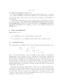
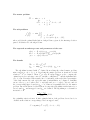
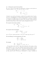
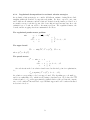
In its optimization mode, DECIS solves two-stage stochastic linear programs with recourse:
min z =
s/t
cx + E f ω y ω
Ax
= b
ω
ω
ω
D y
= dω
−B x +
ω
x,
y
≥ 0, ω ∈ Ω.
where x denotes the first-stage, y ω the second-stage decision variables, c represents the
first-stage and f ω the second-stage objective coefficients, A, b represent the coefficients and
right hand sides of the first-stage constraints, and B ω , Dω , dω represent the parameters of
the second-stage constraints, where the transition matrix B ω couples the two stages. In
the literature Dω is often referred to as the technology matrix or recourse matrix. The
first stage parameters are known with certainty. The second stage parameters are random
parameters that assume outcomes labeled ω with probability p(ω), where Ω denotes the set
of all possible outcome labels.
At the time the first-stage decision x has to be made, the second-stage parameters are
only known by their probability distribution of possible outcomes. Later after x is already
determined, an actual outcome of the second-stage parameters will become known, and
the second-stage decision y ω is made based on knowledge of the actual outcome ω. The
objective is to find a feasible decision x that minimizes the total expected costs, the sum of
first-stage costs and expected second-stage costs.
6
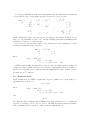
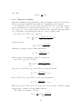
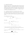
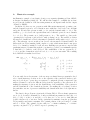
For discrete distributions of the random parameters, the stochastic linear program can
be represented by the corresponding equivalent deterministic linear program:
min z =
s/t
cx + p1 f y 1 + p2 f y 2 +
Ax
Dy 1
−B 1 x +
−B 2 x
+
Dy 2
..
.
···
..
.
−B W x
x,
+ pW f y W
+
y1,
y2,
...,
Dy W
yW
= b
= d1
= d2
..
.
= dW
≥ 0,
which contains all possible outcomes ω ∈ Ω. Note that for practical problems W is very
large, e.g., a typical number could be 1020 , and the resulting equivalent deterministic linear
problem is too large to be solved directly.
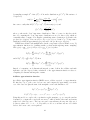
In order to see the two-stage nature of the underlying decision making process the
folowing representation is also often used:
min cx + E z ω (x)
Ax
= b
x
≥ 0
where
z ω (x) = min f ω y ω
Dω y ω = dω + B ω x
y ω ≥ 0, ω ∈ Ω = {1, 2, . . . , W }.
DECIS employs different strategies to solve two-stage stochastic linear programs. It
computes an exact optimal solution to the problem or approximates the true optimal solution very closely and gives a confidence interval within which the true optimal objective
lies with, say, 95% confidence.
3.2.
Evaluation mode
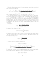
In its evaluation mode, DECIS computes the expected optimal cost, corresponding to a
given first-stage decision x̂, i.e.,
cx̂ + E z ω (x̂),
where
z ω (x̂) = min f ω y ω
Dω y ω = dω + B ω x̂
y ω ≥ 0, ω ∈ Ω = {1, 2, . . . , W },
and
Ax̂ = b.
Note that also in the evaluation model DECIS solves subproblems in order to compute the
expected second-stage cost E z ω (x̂), for given x̂. All different solution strategies available
in the optimization mode can also be employed in the evaluation mode.
7
3.3.
Representing uncertainty
It is favorable to represent the uncertain second-stage parameters in a structure. Using
V = (V1 , . . . , Vh ) an h-dimensional independent random vector parameter that assumes
outcomes v ω = (v1 , . . . , vh )ω with probability pω = p(v ω ), we represent the uncertain secondstage parameters of the problem as functions of the independent random parameter V :
f ω = f (v ω ),
B ω = B(v ω ),
Dω = D(v ω ),
dω = d(v ω ).
Each component Vi has outcomes viωi , ωi ∈ Ωi , where ωi labels a possible outcome of
component i, and Ωi represents the set of all possible outcomes of component i. An outcome
of the random vector
v ω = (v1ω1 , . . . , vhωh )
consists of h independent component outcomes. The set
Ω = Ω1 × Ω2 × . . . × Ωh
represents the crossing of sets Ωi . Assuming each set Ωi contains Wi possible outcomes,
|Ωi | = Wi , the set Ω contains W = Wi elements, where |Ω| = W represents the number of
all possible outcomes of the random vector V . Based on independence, the joint probability
is the product
pω = pω1 1 pω2 2 · · · pωh h .
Let η denote the vector of all second-stage random parameters, e.g., η = vec(f, B, D, d).
The outcomes of η may be represented by the following general linear dependency model:
η ω = vec(f ω , B ω , dω , dω ) = Hv ω ,
ω∈Ω
where H is a matrix of suitable dimensions. DECIS can solve problems with such general
linear dependency models. Section 4 discusses how to input H and v ω .
3.4.
Solving the universe problem
We refer to the universe problem if we consider all possible outcomes ω ∈ Ω and solve
the corresponding problem exactly. This is not always possible, because there may be
too many possible realizations ω ∈ Ω. For solving the problem DECIS employs Benders
decomposition, splitting the problem into a master problem, corresponding to the first-stage
decision, and into subproblems, one for each ω ∈ Ω, corresponding to the second-stage
decision. The details of the algorithm and techniques used for solving the universe problem
are discussed in Section 6.1.
Solving the universe problem is referred to as strategy 4 (istrat = 4) in the parameter
file (see Section 4.4). Use this strategy only if the number of universe scenarios is reasonably
small. There is a maximum number of universe scenarios DECIS can handle, which depends
on your particular installation. If you try to solve a model with more than the maximum
number of universe scenarios, DECIS will stop with an error message.
8
3.5.
Solving the expected value problem
The expected value problem results from replacing the stochastic parameters by their expectation. It is a linear program that can also easily be solved by employing a solver directly.
Solving the expected value problem may be useful by itself (for example as a benchmark to
compare the solution obtained from solving the stochastic problem), and it also may yield
a good starting solution for solving the stochastic problem. DECIS solves the expected
value problem using Benders decomposition. The details of generating the expected value
problem and the algorithm used for solving it are discussed in Section 6.2.
Since in the decomposed mode there is only one (expected value) subproblem, solving
the expected value problem is the fastest strategy that can be used. Therefore when settingup a new model, solving the expected value problem is a good way of getting started and
of finding possible mistakes in your model files.
To solve the expected value problem choose strategy 1 (istrat = 1) in the parameter
input file.
3.6.
Using Monte Carlo sampling
As noted above, for many practical problems it is impossible to obtain the universe solution,
because the number of possible realizations |Ω| is way too large. The power of DECIS lies in
its ability to compute excellent approximate solutions by employing Monte Carlo sampling
techniques. Instead of computing the expected cost and the coefficients and the righthand sides of the Benders cuts exactly (as it is done when solving the universe problem),
DECIS, when using Monte Carlo sampling, estimates the quantities in each iteration using
an independent sample drawn from the distribution of the random parameters. In addition
to using crude Monte Carlo, DECIS uses importance sampling or control variates as variance
reduction techniques.
The details of the algorithm and the different techniques used are described in Section
6.3. You can choose crude Monte Carlo, referred to as strategy 6 (istrat = 6), Monte Carlo
importance sampling, referred to as strategy 2 (istrat = 2), or control variates, referred to
as strategy 10 (istrat = 11). Both Monte Carlo importance sampling and control variates
have been shown for many problems to give a better approximation compared to employing
crude Monte Carlo sampling.
When using Monte Carlo sampling DECIS computes a close approximation to the true
solution of the problem, and estimates a close approximation of the true optimal objective
value. It also computes a confidence interval within which the true optimal objective of
the problem lies, say with 95% confidence. The confidence interval is based on rigorous
statistical theory. An outline of how the confidence interval is computed is given in Section
6.3.4. The size of the confidence interval depends on the variance of the second-stage cost
of the stochastic problem and on the sample size used for the estimation. You can expect
the confidence interval to be very small, especially when you employ importance sampling
or control variates as a variance reduction technique.
When employing Monte Carlo sampling techniques you have to choose a sample size (set
in the parameter file). Clearly, the larger the sample size the better will be the approximate
solution DECIS computes, and the smaller will be the confidence interval for the true
optimal objective value. The default value for the sample size is 100 (nsamples = 100).
9
Setting the sample size too small may lead to bias in the estimation of the confidence
interval, therefore the sample size should be at least 30. There is a maximum value for
the sample size DECIS can handle, which depends on your particular installation. If you
try to choose a larger sample size than the maximum value, DECIS will stop with an error
message.
3.7.
Monte Carlo pre-sampling
We refer to pre-sampling when we first take a random sample from the distribution of the
random parameters and then generate the approximate stochastic problem defined by the
sample. The obtained approximate problem is then solved exactly using decomposition.
This is in contrast to the way we used Monte Carlo sampling in the previous section, where
we used Monte Carlo sampling in each iteration of the decomposition.
The details of the techniques used for pre-sampling are discussed in Section 6.4. DECIS
computes the exact solution of the sampled problem using decomposition. This solution is
an approximate solution of the original stochastic problem. Besides this approximate solution, DECIS computes an estimate of the expected cost corresponding to this approximate
solution and a confidence interval within which the true optimal objective of the original
stochastic problem lies with, say, 95% confidence. The confidence interval is based on statistical theory, its size depends on the variance of the second-stage cost of the stochastic
problem and on the sample size used for generating the approximate problem. In conjunction with pre-sampling no variance reduction techniques are currently implemented.
Using Monte Carlo pre-sampling you have to choose a sample size. Clearly, the larger
the sample size you choose, the better will be the solution DECIS computes, and the smaller
will be the confidence interval for the true optimal objective value. The default value for
the sample size is 100 (nsamples = 100). Again, setting the sample size as too small may
lead to a bias in the estimation of the confidence interval, therefore the sample size should
be at least 30. There is a maximum value for the sample size DECIS can handle, which
depends on your particular installation. If you try to choose a larger sample size than the
maximum value, DECIS will stop with an error message.
For using Monte Carlo pre-sampling choose strategy 8 (istrat = 8) in the parameter file.
3.8.
Regularized decomposition
When solving practical problems, the number of Benders iterations can be quite large.
In order to control the decomposition, with the hope to reduce the iteration count and
the solution time, DECIS makes use of regularization. When employing regularization, an
additional quadratic term is added to the objective of the master problem, representing
the square of the distance between the best solution found so far (the incumbent solution)
and the variable x. Using this term, DECIS controls the distance of solutions in different
decomposition iterations.
For enabling regularization you have to set the corresponding parameters in the parameter file (ireg = 1). You also have to choose the value of the constant rho in the
regularization term. The default is regularization disabled. Details of how DECIS carries
out regularization are represented in Section 6.5.2.
10
Regularization has proven to be especially helpful for problems that need a large number
of Benders iteration when solved without regularization. Problems that need only a small
number of Benders iterations without regularization are not expected to improve much with
regularization, and may need even more iterations with regularization.
4.
Inputting the problem
The DECIS software inputs problems in the SMPS input format. SMPS stands for Stochastic Mathematical Programming System. SMPS, see Birge et al. (1989) [2], is an extension
to the well known MPS (Mathematical Programming System) format, see International
Business Machines (1988) [9], for deterministic problems. The SMPS format uses three files
to define a stochastic problem: the core file, the time file, and the stochastic file.
The core file represents a deterministic version of the stochastic problem in MPS format,
where the random parameters are represented by an arbitrary outcome. Instead of an arbitrary outcome, you may want to put the expected value of each of the stochastic parameters
in the core file. The time file gives pointers as to which variables and constraints belong
to the first stage and which variables and constraints belong to the second stage, using the
names of rows and columns in the core file. The stochastic file contains all the information
about the distribution of the stochastic parameters, where the stochastic parameters are
identified by the row and/or column name as defined in the core file. You may want to use
a modeling language, e.g., GAMS (Brooke, Kendrik, and Meeraus (1988), [3]) or AMPL
(Fourer, Gay and Kernighan (1992) [8]) to formulate the problem and generate the SMPS
input files automatically using the smps.pl program of Entriken and Stone (1997) [7].
In addition, parameters for controlling the execution of DECIS are represented in the
parameter file, the initial seed for the random number generator is inputted via the initial
seed file and, when using MINOS as the optimizer for solving master and subproblems,
parameters to control the execution of MINOS as a subroutine of DECIS are inputted via
the MINOS specification file. DECIS, in evaluation mode, evaluates a particular first-stage
solution. You can input a first-stage solution for evaluation via the free format solution file.
Note the convention for file names: all files specifying a problem and its solution have
the filename “MODEL” and are distinguished by their file extension.
4.1.
The core file
The name of the core file is “MODEL.COR”. The core file represents a deterministic version
of the problem in MPS format. We now give a brief description of how to implement a
problem in the MPS format. In the MPS format variable names and constraint names
may have up to eight characters of length. The core filecontaines the following cards and
sections:
1. The NAME card — It has to be the first record of the file and contains the word
“NAME” in the format (A4). After “name” you have 20 characters to write any
information you want to identify the file. This information will appear then on the
solution output of the solver.
2. The ROWS card — Initializes the rows section of the problem. It has to be the second
record and contains the name “ROWS” in the format (A4). It is followed by
11
3. The Rows section — It contains the constraint names and the relation between the
left hand side and the right hand side of each constraint. Use one record for each
constraint in the format (1X, A1, 2X, A8), which means keep the first digit free, then
use one digit for the relation between left hand and right hand side of the constraint,
keep two digits free, and use up to 8 digits for the constraint name. Constraint names
can consist of any characters and numbers including the special characters of the
ASCII character set. For the relations between the left hand side and right hand side
of the constraints use “E” for equal, “G” for greater equal, and “L” for less equal.
The first row in the list has to be the objective function. The objective function is
a free row, denoted by the relation sign “N”. It is important that you input all first
stage constraint names first and all second stage constraints thereafter. Within the
first stage constraints and within the second stage constraints you may enter the rows
in any order.
4. The COLUMNS card — Initializes the columns section of the problem. It has to
follow the rows section and contains the name “COLU” in the format (A4). You
can also write “COLUMNS”, but only the first 4 characters will be processed. It is
followed by
5. The Columns section — It contains the coefficients of the linear constraints. Only nonzero coefficients have to be considered and you can leave out the zero coefficients of the
constraints. You can input the coefficients in the one or two column representation
of the MPS format. In the one column representation, each record corresponds to
one coefficient and has the format (4X, A8, 2X, A8, 2X, E12.0), which means, leave
the first 4 digits blank, use the following 8 digits for the variable name, leave 2 digits
blank, use the following 8 digits for the constraint name, leave 2 digits empty, and
use up to 12 digits for the decimal representation of the non zero coefficient. In the
two column representation, each record corresponds to two coefficients and has the
format (4X, A8, 2X, A8, 2X, E12.0, 2X, A8, 2X, E12.0). You can represent another
coefficient corresponding to the variable and another row in the same record. Leave
after the first row name 2 digits blank, use the following 8 digits for another row
name, leave 2 digits blank, and use up to 12 digits for the decimal representation
of the non zero coefficient corresponding to the latter row name. You have to input
the coefficients grouped by each variable, meaning in the order that all coefficients
corresponding to a certain variable come one after the other. You can not switch
between variables in the sense that you input some coefficients corresponding to one
variable, then input some coefficients of another variable, and then again coefficients
of the former variable. It is important that you input all first stage variables first and
all second stage variables thereafter. Within the set of first stage variables and within
the set of second stage variables you can input variables in any order you wish. The
constraint names and corresponding coefficients associated with a variable can be in
any order. Corresponding to each variable you do not need to input first stage row
names and corresponding coefficients before second stage variables and corresponding
coefficients. After the columns section follows
6. The RHS card — It initializes the right hand side section of the constraint. It has to
12
follow the columns section and contains the name “RHS ” in the format (A4). It is
followed by
7. The right hand side section — It contains the values of the right hand sides of the
constraints if they are non zero. You can leave out the right hand sides which are
zero. There is one record for each non-zero right hand side in the format (4X, A8,
2X, A8, 2X, E12.0), which means leave the first 4 digits empty, then use 8 digits to
represent a generic name for all the right hand sides (it has to be the same name for
all right hand sides), then use 8 digits for the constraint name, leave 2 digits empty,
and use up to 12 digits for the decimal representation of the right hand side value of
the corresponding right hand side. You can choose any name for all your right hand
sides, e.g., “RHS ” would be a proper name.
8. The RANGES card — It initializes the ranges section, which is used to input ranges
on the right-hand side of rows. It has to follow directly the right hand side section
and contains the name “RANG” in the format (A4). You can also write ”RANGES”,
but only the first 4 characters will be processed. It is followed by
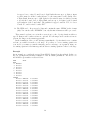
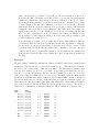
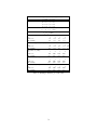
9. The ranges section – It contains the ranges of the right-hand sides of rows. Ranges
determine upper and lower bounds on rows, the exact meaning depends on the type
of the row and the sign of the right-hand side. The following table gives the resulting
lower and upper bound of a row depending on its type and the sign of its right-hand
side, where b denotes the value of the right-hand side and r the value of the range
inputted in the ranges section.
row type right-hand side sign lower bound upper bound
E
+
b
b + |r|
E
−
b − |r|
b
G
+ or −
b
b + |r|
L
+ or −
b − |r|
b
The format is (4X, A8, 2X, A8, 2X, E12.0), which means leave the first 4 digits
empty, then use 8 digits to represent a generic name for all the ranges (it has to be
the same name for all ranges), then use 8 digits for the constraint name, leave 2 digits
empty, and use up to 12 digits for the decimal representation of the range value of
the corresponding right hand side. You can choose any name for all your ranges, e.g.,
“RANGES ” would be a proper name.
10. The BOUNDS card — It initializes the bounds section, which is used to input bounds
on the value of the variables. It has to follow the right hand side section and contains
the name “BOUN” in the format (A4). You can also write ”BOUNDS”, but only the
first 4 characters will be processed. It is followed by
11. The bounds section — It contains the values of the bounds on the variables. You can
specify upper bounds, lower bounds and fixed bounds on any of the variables defined
in the columns section in any order. The format is (1X, A2, 1X, A8, 2X, A8, 2X,
E12.0), which means leave the first digit blank, then use 2 digits to input the qualifier
13
for upper, lower, or fixed bound, leave 1 digit blank, then use up to 8 digits to input
a generic name for all the bounds (it has to be the same name for all bounds), leave
2 digits blank, then use up to eight digits for the variable name for which you want
to specify the bound, leave 2 digits blank, and use up to 12 digits for the decimal
representation of the bound value. The qualifier for upper bounds is “UP”, for lower
bounds “L”, and for fixed bounds “FX”.
12. The END card — Reports end of data and contains the name “ENDA” in the format
(A4). You can also write “ENDATA”, but only the first 4 characters will be processed.
There must be at least one row in the rows section, i.e., the objective function with row
type N. Ranges and bounds sections are optional. If both ranges and bounds sections are
present, the ranges section must appear first.
In the formulation of the core file, it is important that the objective function row contains
at least one variable from the second stage. If you have a cost accounting equation in
your model, you must account the first-stage and second-stage cost separately using one
accounting equation for the first stage and another accounting equation for the second stage.
Example
As an example we consider the test problem APL1P, discussed in Appendix A. In the core
file you can input any arbitrary realization of the stochastic parameters. The model core
file in MPS representation reads as follows:
NAME
ROWS
N ZFZF9999
G A0000001
G A0000002
L F0000001
L F0000002
G D0000001
G D0000002
G D0000003
COLUMNS
X0000001
X0000001
X0000001
X0000002
X0000002
X0000002
Y0000011
Y0000011
Y0000011
Y0000012
Y0000012
Y0000012
Y0000013
Y0000013
Y0000013
Y0000021
Y0000021
APL1P
ZFZF9999
A0000001
F0000001
ZFZF9999
A0000002
F0000002
ZFZF9999
F0000001
D0000001
ZFZF9999
F0000001
D0000002
ZFZF9999
F0000001
D0000003
ZFZF9999
F0000002
4.00000E+00
1.00000E+00
-1.00000E+00
2.50000E+00
1.00000E+00
-1.00000E+00
4.30000E+00
1.00000E+00
1.00000E+00
2.00000E+00
1.00000E+00
1.00000E+00
0.50000E+00
1.00000E+00
1.00000E+00
8.70000E+00
1.00000E+00
14
Y0000021
Y0000022
Y0000022
Y0000022
Y0000023
Y0000023
Y0000023
UD000001
UD000001
UD000002
UD000002
UD000003
UD000003
D0000001
ZFZF9999
F0000002
D0000002
ZFZF9999
F0000002
D0000003
ZFZF9999
D0000001
ZFZF9999
D0000002
ZFZF9999
D0000003
1.00000E+00
4.00000E+00
1.00000E+00
1.00000E+00
1.00000E+00
1.00000E+00
1.00000E+00
1.00000E+01
1.00000E+00
1.00000E+01
1.00000E+00
1.00000E+01
1.00000E+00
A0000001
A0000002
F0000001
F0000002
D0000001
D0000002
D0000003
1.00000E+03
1.00000E+03
0.000000+00
0.000000+00
1.00000E+03
1.00000E+03
1.00000E+03
RHS
RHS
RHS
RHS
RHS
RHS
RHS
RHS
ENDATA
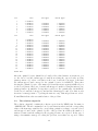
In the example, “ZFZF9999” is the objective function row; “A0000001” and “A0000002”
are first stage rows; “F0000001”, F0000002”, ”D0000001”, ”D0000002”, and ”D0000003”
are second stage rows; “X0000001” and “X0000002” are first stage variables; “Y0000011”,
. . ., “UD000003” are second stage variables. As a generic right hand side name “RHS ” was
used.
In the core file the value 1000.0 was inputted for each of the stochastic demands di ,
i = 1, 2, 3, and the value 1.0 was inputted for the stochastic availability of the generators
βj , j = 1, 2. These values serve only as a place holder for non zero values. They are not
further processed and have no impact on the solution. The distribution of the stochastic
demands and the distribution of the availability of generators is inputted in the stochastic
file described below. However, you can easily read all deterministic data of the problem
from the core MPS file.
4.2.
The time file
The name of the time file is “MODEL.TIM”. The time file is used to specify which variables
and constraints belong to the first stage and which to the second stage. It closely mimics
the MPS format for inputting variable names and row names. It consists of the following
cards and sections:
1. The TIME card — It has to be the first record of the file and contains the word
“TIME” in the format (A4). After “name” you have 20 characters to write any
information you want to identify the file. This information is for your records only
and will not be further processed.
2. The PERIODS card — It contains the word “PERI” in the format (A4). You can
also specify “PERIODS”, but only the first four characters will be processed. The
PERIODS card initializes
15
3. The periods section — It defines the first stage and the second stage variables and
constraints through pointers to the first row and first column of each stage. There is
one card for each stage in the format (4X, A8, 2X, A8, 16X, A8), which means leave
the first 4 digits blank, then use up to 8 digits for the first column name, leave 2 digits
blank, the use up to 8 digits for the first row name, leave 16 digits blank, and use up
to 8 digits to indicate which stage the pointer refers to. The latter stage indicator is
for your information only and is not further processed. The cards must be in order.
You have to input the card for the first stage pointers first, followed by the card for
the second stage pointers.
4. The END card – Reports end of data and contains the name “ENDA” in the format
(A4). You can also write “ENDATA”, but only the first four characters will be
processed.
Note that the first row of the first stage constraints is the objective function, since
the DECIS system treats the objective function as just another constraint. This may be
different from other software packages solving stochastic problems, where the objective
function is treated separately. These packages then require the first row name of the first
stage constraints to be the “real” first row of the constraint matrix.
We have limited the discussion here to specifying two stages only. The SMPS format is
able to specify multi-stage problems with more than two stages. For a description of the
time file for more than two stages, please see Birge et al. (1989) [2].
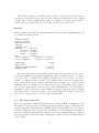
Example
For the example of the stochastic electric power planning problem, APL1P, the corresponding time file is as follows:
TIME
APL1P
PERIODS
LP
X0000001 ZFZF9999
Y0000011 F0000001
ENDATA
PERIOD1
PERIOD2
“X000001” is the first of the first stage columns and “ZFZF9999” is the first of the first
stage constraints; “Y0000011” is the first of the second stage columns, and “F0000001” is
the first of the second stage constraints.
4.3.
The stochastic file
The name of the stochastic file is “MODEL.STO”. The stochastic file is used to specify the
distribution of the stochastic parameters. The stochastic parameters are identified by the
corresponding row and column names in the core file. The input format of the stochastic file
mimics closely the MPS format for inputting row and column names and the corresponding
parameters. In the current implementation of the DECIS system, we consider only discrete
random parameters. Note that you can closely approximate continuous random parameters
by discrete ones using a sufficient number of discrete realizations. However, there are plans
to provide also for certain continuous random parameters (normal, uniform, and others)
16
in the near future. DECIS can handle both, independent random parameters and certain
types of dependent random parameters. The stochastic file consists of the following cards
and sections:
1. The NAME card — It has to be the first record of the file and contains the word
“NAME” in the format (A4). After “NAME” you have 20 characters to write any
information you want to identify the file. This information is only for your records
and will not be further processed.
2. The INDEPENDENT card — It contains the word “INDE” and a qualifier for the
distribution in the format (A4, 10X, A8), which means input the word “INDE”,
leave 10 digits blank, and then use 8 digits for the distribution qualifier. Since we
currently only provide for discrete distributions the only valid qualifier is the word
“DISCRETE” Instead of “INDE” you can also specify “INDEPENDENT”, but only
the first 4 characters will be processed. (The first character of the word “DISCRETE”
always has to be the 15-th digit of the record.) The independent card initializes
3. The independent section — It is used to specify all independent random parameters of
the problem. Use one record for each possible realization of a random parameter and
input the different independent random parameters one after the other. You cannot
specify some realizations of one random parameter, then continue with inputting
realization of another random parameter, and then continue inputting realizations of
the first random parameter. The random parameters are identified by 2 identifiers. If
the random parameter is a B matrix or a D matrix (including the objective function)
coefficient the first identifier is the column name and the second identifier is the row
name of that random coefficient. If the random parameter is a right-hand side value
the first identifier is the right-hand side name in the core file (e.g., the string “RHS”)
and the second identifier is the row name of that right-hand side coefficient. If the
uncertain parameter is a bound value (lower upper or fixed bound) the first identifier
is the string “BND” and the second identifier is the column name of that bound
coefficient. For specifying bounds we also need the keywords “LO” (for lower bound),
“UP” (for upper bound), or “FX” (for fixed bound), which are in colums 3 and 4 of
the record. The format for specifying a possible realization is (1X, A2, 1X, A8, 2X,
A8, 2X, E12, 2X, A8, 2X, E12), which means leave the first digit blank, use two digits
for the keyword (bounds only), leave one digit blank, then use up to 8 digits to enter
the first identifier, leave 2 digits blank, then use up to eight digits to specify the second
identifier, leave 2 digits blank, use up to 12 digits for the decimal representation of the
value of the realization, leave 2 digits blank, use 8 digits to identify the stage at which
the realization will become known, leave 2 digits blank, and use up to 12 digits for the
decimal representation of the probability with which the realization occurs. The stage
identifier is for your information only, and it is not further processed. Since we are
concerned with two stage problems only, all random parameter realizations become
known in the second stage. The probabilities of the different possible realizations of
each random parameter should sum up to one. If for a particular random parameter
the probabilities don’t sum to one, DECIS divides the probability of each realization
of that random parameter by the sum of the probabilities of all possible realizations
17
of that random parameter.
4. The BLOCKS card — It contains the word “BLOC” and a qualifier for the distribution
in the format (A4, 10X, A8), which means input the word “BLOC”, leave 10 digits
blank, and then use 8 digits for the distribution qualifier. Since we currently only
provide for discrete distributions the only valid qualifier is the word “DISCRETE”.
Instead of “BLOC” you can also specify “BLOCKS”, but only the first 4 characters
will be processed. The blocks card initializes a whole section used to specify all dependent random parameters of the problem. DECIS considers additive dependency.
Dependent random parameters are represented as additive functions of one or several
independent random parameters. The independent random parameters are called
blocks. For each possible realization of a block, the coefficients for each of the dependent random parameters are specified. You can view these coefficients as the product
of the outcome of the independent random parameter times the factor corresponding
to the dependent random parameter.
5. The BL card — Initializes a possible realization of a block of random parameters. It
has the format (1X, A2, 1X, A8, 2X, A8, 2X, E12), which means leave the first digit
blank, use 2 digits to input the block identifier “BL”, leave one digit blank, use up
to 8 digits to input the block name, leave 2 digits blank, use up to 8 digits to specify
the stage identifier, leave 2 digits blank and then use up to 12 digits for the decimal
representation of the probability corresponding to the realization of the block. The
stage identifier is for your information only, it is not further processed.
6. The BL section — It is used to specify all random parameters realizations of the
block named in the “BL” card. Use one record for each dependent random parameter
realization and input the different dependent random parameters one after the other.
Like in the independent section, the random parameters are identified by 2 identifiers.
If the random parameter is a B matrix or a D matrix (including the objective function)
coefficient the first identifier is the column name and the second identifier is the row
name of that random coefficient. If the random parameter is a right-hand side value
the first identifier is the right-hand side name in the core file (e.g., the string “RHS”)
and the second identifier is the row name of that right-hand side coefficient. If the
uncertain parameter is a bound value (lower, upper or fixed bound) the first identifier
is the string “BND” and the second identifier is the column name of that bound
coefficient. For specifying bounds we also need the keywords “LO” (for lower bound),
“UP” (for upper bound), or “FX” (for fixed bound), which are in colums 3 and 4 of
the record. The format for specifying a possible realization is (1X, A2, 1X, A8, 2X,
A8, 2X, E12, 2X, A8, 2X, E12), which means leave the first digit blank, use two digits
for the keyword (bounds only), leave one digit blank, then use up to 8 digits to enter
the first identifier, leave 2 digits blank, then use up to eight digits to specify the second
identifier, leave 2 digits blank, use up to 12 digits for the decimal representation of
the value of the realization.
After having inputted all dependent realizations associated with a certain outcome of
the block, initialize a new realization of the block with corresponding probability using
a new “BL” card. To specify a new realization of the same block, keep the same block
18
name, but input the probability corresponding to the new realization of the block.
Following the “BL” card input a new “BL section” to specify all dependent random
parameters realizations corresponding to the new realization of the block. When
specifying the first realization of a block you must input all coefficients corresponding
to that realization. For any other realization, you only need to specify the coefficients
that change from the previous realization. You do not have to input coefficients that
remain the same from the previous realization. The values that don’t change are
updated automatically. For all realizations of a block, the probabilities should sum
up to one. If for a particular block the probabilities don’t sum to one, DECIS divides
the probability of each realization of that block by the sum of the probabilities of all
possible realizations of that block.
You can specify more than one block. Different blocks are distinguished by different
block names. Each block is treated as an independent random parameter. Using the
block section you can specify any additive dependency model: If two or more blocks
contain the same dependent random parameter the coefficients of each of the outcomes
of the blocks are added. A particular realization of a dependent random parameter is
then generated as the the sum of the realizations of independent random parameters
(blocks).
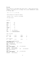
Examples
The first example considers the distribution of the model APL1P with 5 independent random
parameters. The first and the second random parameter are coefficients in the B matrix,
specified by the corresponding column and row names. The first random parameter has
four outcomes, namely (-1, -0.9. -0.5, -0.1) with corresponding probabilities (0.2, 0.3, 0.4,
0.1), the second random parameter has five outcomes, namely (-1.0, -0.9, -0.7, -0.1, 0.0)
with corresponding probabilities (0.1, 0.2, 0.5, 0.1, 0.1). The third, fourth and fifth random
parameter are right hand side values, identified by the identifier “RHS ” and the row name of
the random right hand side. All three right hand sides are identically distributed with four
different discrete outcomes, namely (900, 1000, 1100, 1200) with corresponding probabilities
(0.15, 0.45, 0.25, 0.15). The five independent random parameters give rise to 4*5*4*4*4 =
1280 possible combinations of different realizations. The stochastic file looks as follows:
NAME
INDEP
X0000001
X0000001
X0000001
X0000001
*
X0000002
X0000002
X0000002
X0000002
X0000002
*
RHS
RHS
APL1P
DISCRETE
F0000001
F0000001
F0000001
F0000001
-1.0
-0.9
-0.5
-0.1
PERIOD2
PERIOD2
PERIOD2
PERIOD2
0.2
0.3
0.4
0.1
F0000002
F0000002
F0000002
F0000002
F0000002
-1.0
-0.9
-0.7
-0.1
-0.0
PERIOD2
PERIOD2
PERIOD2
PERIOD2
PERIOD2
0.1
0.2
0.5
0.1
0.1
D0000001
D0000001
900.0
1000.0
PERIOD2
PERIOD2
0.15
0.45
19
RHS
RHS
D0000001
D0000001
1100.0
1200.0
PERIOD2
PERIOD2
0.25
0.15
RHS
RHS
RHS
RHS
D0000002
D0000002
D0000002
D0000002
900.0
1000.0
1100.0
1200.0
PERIOD2
PERIOD2
PERIOD2
PERIOD2
0.15
0.45
0.25
0.15
RHS
RHS
RHS
RHS
ENDATA
D0000003
D0000003
D0000003
D0000003
900.0
1000.0
1100.0
1200.0
PERIOD2
PERIOD2
PERIOD2
PERIOD2
0.15
0.45
0.25
0.15
*
*
The second example considers 3 independent random parameters. Tthe first two are the
same as above, and the third one is called “BLOCK1” and is a block controlling the outcomes
of 3 dependent random parameters. The three dependent random parameters are right
hand side values, specified by the identifier “RHS” and the row name of the corresponding
random right hand side. The block has two outcomes, each occurring with probability 0.5.
For the first outcome the three dependent demands “D0000001”,“D0000002”,“D0000003”
take on the values 1100, 1100, 1100, and for the second outcome the values 900, 900, 900,
respectively. The two independent random parameters and the independent block generate
4*5*2 = 40 possible combinations of realizations. There are two independent and three
dependent random variables specified in the example. The corresponding stochastic file is:
NAME
INDEP
X0000001
X0000001
X0000001
X0000001
X0000002
X0000002
X0000002
X0000002
X0000002
BLOCKS
BL BLOCK1
RHS
RHS
RHS
BL BLOCK1
RHS
RHS
RHS
ENDATA
APL1PC
DISCRETE
F0000001
F0000001
F0000001
F0000001
F0000002
F0000002
F0000002
F0000002
F0000002
DISCRETE
PERIOD2
D0000001
D0000002
D0000003
PERIOD2
D0000001
D0000002
D0000003
-1.0
-0.9
-0.5
-0.1
-1.0
-0.9
-0.7
-0.1
-0.0
PERIOD2
PERIOD2
PERIOD2
PERIOD2
PERIOD2
PERIOD2
PERIOD2
PERIOD2
PERIOD2
0.2
0.3
0.4
0.1
0.1
0.2
0.5
0.1
0.1
0.5
1100.0
1100.0
1100.0
0.5
900.0
900.0
900.0
The third example shows how to specify a general additive dependency model using
blocks. Suppose there are two independent random parameters driving the electric power
demand, e.g., temperature and economic activity. These independent random parameters
are referred to as “BLOCK1” and “BLOCK2”. Each of these blocks has 2 realizations,
“BLOCK1” with corresponding probabilities 0.5, and 0.5; “BLOCK2”with corresponding
20
probabilities 0.2, and 0.8. Each of the blocks controls the same dependent random parameters “D0000001”,“D0000002”,“D0000003”. “BLOCK1” in its first realization generates
right hand side values of (1100, 900, 500), and in its second realization the values (300, 400,
200); “BLOCK2” in its first realization the values (200, 300, 500) and in its second realization the values (100, 150, 300). When generating realizations, DECIS adds the coefficients
of the dependent random parameters regarding different blocks. In the example, there are
2*2 = 4 possible combinations of realizations of the dependent parameters, namely (1300,
1200, 1000), (1000, 1050, 800), (500, 700, 700), and (400, 550, 500), generated as the sum
of the coefficients for each of the two blocks. The corresponding stochastic file reads as
follows:
NAME
BLOCKS
BL BLOCK1
RHS
RHS
RHS
BL BLOCK1
RHS
RHS
RHS
BL BLOCK2
RHS
RHS
RHS
BL BLOCK2
RHS
RHS
RHS
ENDATA
4.4.
APL1PCA
DISCRETE
PERIOD2
D0000001
D0000002
D0000003
PERIOD2
D0000001
D0000002
D0000003
PERIOD2
D0000001
D0000002
D0000003
PERIOD2
D0000001
D0000002
D0000003
0.5
1100.0
900.0
500.0
0.5
300.0
400.0
200.0
0.2
200.0
300.0
500.0
0.8
100.0
150.0
300.0
The parameter file
In the parameter input file you can specify parameters regarding the solution algorithm
used and control the output of the DECIS program. There is a record for each parameter
you want to specify. Each record consists of the value of the parameter you want to specify
and the keyword identifying the parameter, separated by a blank character or a comma.
You may specify parameters with the following keywords: “istrat”, “nsamples”, “nzrows”,
“maxit”, “iwrite”, “ibug”, “iscratch”, “iresamp”, “iappr”, “ireg”, “rho”, “tolben”, and
“tolw” in any order. Each keyword can be specified in lower case or upper case text in the
format (A10). Since DECIS reads the records in free format you don’t have to worry about
the format, but some computers require that the text is inputted in quotes. Parameters
that are not specified in the parameter file automatically assume their default values.
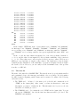
istrat — Defines the solution strategy used. The default value is istrat = 3.
istrat = 1 Solves the expected value problem. All stochastic parameters are replaced
by their expected values and the corresponding deterministic problem is solved
using decomposition.
21
istrat = 2 Solves the stochastic problem using Monte Carlo importance sampling.
You have to additionally specify what approximation function you wish to use,
and the sample size used for the estimation, see below.
istrat = 3 Refers to istrat = 1 plus istrat = 2. First solves the expected value
problem using decomposition, then continues and solves the stochastic problem
using importance sampling.
istrat = 4 Solves the stochastic universe problem by enumerating all possible combinations of realizations of the second-stage random parameters. It gives you
the exact solution of the stochastic program. This strategy may be impossible,
because there may be way too many possible realizations of the random parameters. There is a maximum number of possible universe scenarios DECIS can
solve, which is defined at compilation.
istrat = 5 Refers to istrat = 1 plus istrat = 4. First solves the expected value problem
using decomposition, then continues and solves the stochastic universe problem
by enumerating all possible combinations of realizations of second-stage random
parameters.
istrat = 6 Solves the stochastic problem using crude Monte Carlo sampling. No
variance reduction technique is applied. This strategy is especially useful if you
want to test a solution obtained by using the evaluation mode of DECIS. You
have to specify the sample size used for the estimation. There is a maximum
sample size DECIS can handle. However, this maximum sample size does not
apply when using crude Monte Carlo. Therefore, in this mode you can specify
very large sample sizes, which is useful when evaluating a particular solution.
istrat = 7 Refers to istrat = 1 plus istrat = 6. First solves the expected value
problem using decomposition, then continues and solves the stochastic problem
using crude Monte Carlo sampling.
istrat = 8 Solves the stochastic problem using Monte Carlo pre-sampling. A Monte
Carlo sample out of all possible universe scenarios, sampled from the original
probability distribution, is taken, and the corresponding “sample problem” is
solved using decomposition.
istrat = 9 Refers to istrat = 1 plus istrat = 10. First solves the expected value
problem using decomposition, then continues and solves the stochastic problem
using Monte Carlo pre-sampling.
istrat = 10 Solves the stochastic problem using control variates. You also have to
specify what approximation function and what sample size should be used for
the estimation.
istrat = 11 Refers to istrat = 1 plus istrat = 8. First solves the expected value
problem using decomposition, then continues and solves the stochastic problem
using control variates.
nsamples — Sample size used for the estimation. It should be set greater or equal to 30
in order to fulfill the assumption of large sample size used for the derivation of the
probabilistic bounds. The default value is nsamples = 100.
22
nzrows — Number of rows reserved for cuts in the master problem. It specifies the maximum number of different cuts DECIS maintains during the course of the decomposition algorithm. DECIS adds one cut during each iteration. If the iteration count
exceeds nzrows, then each new cut replaces a previously generated cut, where the cut
is replaced that has the maximum slack in the solution of the (pseudo) master. If
nzrows is specified as too small then DECIS may not be able to compute a solution
and stops with an error message. If nzrows is specified as too large the solution time
will increase. As an approximate rule set nzrows greater than or equal to the number
of first-stage variables of the problem. The default value is nzrows = 100.
maxit — Specifies the maximum number of Benders iterations DECIS uses for solving
the problem. After maxit is reached, DECIS stops the decomposition algorithm and
reports the best solution found so far. The default value is maxit = 1000.
iwrite — Specifies whether the optimizer invoked for solving subproblems writes output
or not. The default value is iwrite = 0.
iwrite = 0 No optimizer output is written.
iwrite = 1 Optimizer output is written to the file “MODEL.MO”. The output level
of the output can be specified using the optimizer options. It is intended as a
debugging device. If you set iwrite = 1, for every master problem and for every
subproblem solved the solution output is written. For large problems and large
sample sizes the file“MODEL.MO” may become very large, and the performance
of DECIS may slow down.
ibug — Specifies the detail of debug output written by DECIS. The output is written
to the file “MODEL.SCR”, but can also be redirected to the screen by a separate
parameter. The higher you set the number of ibug the more output DECIS will
write. The parameter is intended to help debugging a problem and should be set to
ibug = 0 for normal operation. For large problems and large sample sizes the file
“MODEL.SCR” may become very large, and the performance of DECIS may slow
down. The default value is ibug = 0.
ibug = 0 This is the setting for which DECIS does not write any debug output.
ibug = 1 In addition to the standard output, DECIS writes the solution of the master
problem on each iteration of the Benders decomposition algorithm. Thereby
it only writes out variable values which are nonzero. A threshold tolerance
parameter for writing solution values can be specified, see below.
ibug = 2 In addition to the output of ibug = 1, DECIS writes the scenario index and
the optimal objective value for each subproblem solved. In the case of solving
the universe problem, DECIS also writes the probability of the corresponding
scenario.
ibug = 3 In addition to the output of ibug = 2, DECIS writes information regarding
importance sampling. In the case of using the additive approximation function,
it reports the expected value for each i-th component of Γ̄i , the individual sample sizes Ni , and results from the estimation process. In the case of using the
23
multiplicative approximation function it writes the expected value of the approximation function Γ̄ and results from the estimation process.
ibug = 4 In addition to the output of ibug = 3, DECIS writes the optimal dual
variables of the cuts on each iteration of the master problem.
ibug = 5 In addition to the output of ibug = 4, DECIS writes the coefficients and
the right-hand side of the cuts on each iteration of the decomposition algorithm.
In addition it checks if the cut computed is a support to the recourse function
(or estimated recourse function) at the solution x̂k at which it was generated.
If it turns out that the cut is not a support, DECIS writes out the value of the
(estimated) cut and the value of the (estimated) second stage cost at x̂k .
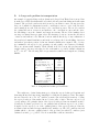
ibug = 6 In addition to the output of ibug = 5, DECIS writes a dump of the
master problem and the subproblem in MPS format after having decomposed
the problem specified in the core file. The dump of the master problem is written
to the file “MODEL.FST” and the dump of the subproblem is written to the file
“MODEL.SND”. DECIS also writes a dump of the original problem, as it was
read from the core file, to the file “MODEL.ORI”.
ibug = 7 In addition to the output of ibug = 6, DECIS writes out information about
the right-hand side vector passed to the subproblem, i.e., the values of bω , the
product of B ω x̂k and the resulting right-hand side bω + B ω x̂k .
ibug = 8 In addition to the output of ibug = 7, DECIS echoes the information it
read when inputting the stochastic file (“MODEL.STO”) into the file “MODEL.
SPR”, and writes out on each iteration of the decomposition algorithm and for
each subproblem solved the index of the realization of each random parameter
that made up the scenario of the subproblem.
iscratch — Specifies the internal unit number to which the standard and debug output is
written. The default value is iscratch = 17, where the standard and debug output is
written to the file “MODEL.SCR”. Setting iscratch = 6 redirects the output to the
screen. Other internal unit numbers could be used, e.g., the internal unit number of
the printer, but this is not recommended. The default value is iscratch = 17.
iresamp — Specifies weather DECIS evaluates the optimal solution using an independent
sample or not, in order to compute an independent upper bound on the optimal
objective of the problem. The parameter is only relevant when you use a solution
strategy where Monte Carlo sampling is involved, i.e., istrat = 2, 3, 6, 7, 8, 9, 10, or
11. The default value is iresamp = 1.
iresamp = 0 The solution found is not evaluated using an independent sample. This
setting is for debugging purposes only and should not be used for actual problem
solving.
iresamp = 1 After completion of the decomposition algorithm DECIS draws an independent sample using the sampling strategy specified and independently evaluates the solution found to compute a probabilistic upper bound.
24
iappr — Specifies the type of approximation function used for carrying out importance
sampling or control variates. The parameter is only relevant for solution strategies
istrat = 2, 3, 10 and 11. The default value is iappr = 1.
iappr = 1 Specifies that the additive marginal cost model is used.
iappr = 2 Specifies that the multiplicative marginal cost factor model is used.
ireg — Specifies whether or not DECIS uses regularized decomposition for solving the
problem. This option is considered if MINOS is used as a master and subproblem
solver, and is not considered if using CPLEX, since regularized decomposition uses a
nonlinear term in the objective. The default value is ireg = 0.
ireg = 1 Specifies that regularized decomposition is used.
ireg = 0 Specifies that no regularization is used.
rho — Specifies the value of the ρ parameter of the regularization term in the objective
function. You will have to experiment to find out what value of rho works best for
the problem you want to solve. There is no rule of thumb as to what value should
be chosen. In many cases it has turned out that regularized decomposition reduces
the iteration count if standard decomposition needs a large number of iterations. The
default value is rho = 1000.
tolben — Specifies the tolerance for stopping the decomposition algorithm. The parameter
is especially important for deterministic solution strategies, i.e., 1, 4, 5, 8, and 9.
Choosing a very small value of tolben may result in a significantly increased number
of iterations when solving the problem. The default value is 10−7 .
tolw — Specifies the nonzero tolerance when writing debug solution output. DECIS writes
only variables whose values are nonzero, i.e., whose absolute optimal value is greater
than or equal to tolw. The default value is 10−9 .
Example
In the following example the parameters istrat = 7, nsamples = 200, nzrows = 200, and
maxit = 3000 are specified. All other parameters are set at their default values. DECIS
first solves the expected value problem and then the stochastic problem using crude Monte
Carlo sampling with a sample size of nsamples = 200. DECIS reserves space for a maximum
of nzrows = 50 cuts. The maximum number of Benders iterations is specified as maxit =
3000.
7
200
50
3000
"ISTRAT"
"NSAMPLES"
"NZROWS"
"MAXIT"
25
4.5.
The initial seed file
In the initial seed file you specify the initial seed for the pseudo random number generator
used in DECIS, and the number of times you want to solve the problem. The name of the
initial seed file is “MODEL.ISE”. It consists of only two lines, where the first line contains
in free format the value of the parameter iseed, and the second line in free format the value
of the parameter irep.
iseed — Specifies the initial seed given to the pseudo random parameter. You can specify
any integer number greater than 0 and less than 2147483647.
irep — Specifies the number of times you want to solve the problem in one run of DECIS.
DECIS has the option of solving a problem repeatedly many times with different seeds,
in order to be able to collect statistics about the solutions and the probabilistic bounds
obtained from the individual runs. The feature is important when using Monte Carlo
sampling based strategies for solving the problem. The outputs of the individual runs
are reported in the file “MODEL.REP”.
Example
In the following example an initial seed of iseed = 12783452, and a number of irep = 1 is
specified. DECIS only reads the first number in each record; you can use the remainder of
each record to write any comments you wish to add. They will not be processed.
12783452
1
4.6.
ISEED: INITIAL SEED
IREP: # OF REPLICATIONS
The MINOS specification file
When you use MINOS as the optimizer for solving the master and the subproblems, you
must specify optimization parameters in the MINOS specification file “MINOS.SPC”. Each
record of the file corresponds to the specification of one parameter and consists of a keyword
and the value of the parameter in free format. Records having a “*” as their first character
are considered as comment lines and are not further processed. For a detailed description
of these parameters, see the MINOS Users’ Guide (Murtagh and Saunders (1983) [13]. The
following parameters should be specified with some consideration:
AIJ TOLERANCE — Specifies the nonzero tolerance for constraint matrix elements of
the problem. Matrix elements aij that have a value for which |aij | is less than “AIJ
TOLERANCE” are considered by MINOS as zero and are automatically eliminated
from the problem. It is wise to specify “AIJ TOLERANCE 0.0 ”
SCALE — Specifies MINOS to scale the problem (“SCALE YES”) or not (“SCALE NO”).
It is wise to specify “SCALE NO”.
ROWS — Specifies the number of rows in order for MINOS to reserve the appropriate
space in its data structures when reading the problem. “ROWS” should be specified
as the number of constraints in the core problem or greater. MINOS terminates with
an error message if “ROWS” is specified to small to read the problem, or if MINOS
is not compiled for a problem the size asked for in the specification file.
26
COLUMNS — Specifies the number of columns in order for MINOS to reserve the appropriate space in its data structures when reading the problem. “COLUMNS” should be
specified as the number of variables in the core problem or greater. MINOS terminates
with an error message if “COLUMNS” is specified too small to read the problem, or
if MINOS is not compiled for a problem the size asked for in the specification file.
ELEMENTS — Specifies the number of nonzero matrix coefficients in order for MINOS
to reserve the appropriate space in its data structures when reading the problem.
“ELEMENTS” should be specified as the number of nonzero matrix coefficients in the
core problem or greater. MINOS terminates with an error message if “ELEMENTS”
is specified to small to read the problem, or if MINOS is not compiled for a problem
the size asked for in the specification file.
Example
The following example represents typical specifications for running DECIS with MINOS as
the optimizer.
BEGIN SPECS
PRINT LEVEL
1
LOG FREQUENCY
10
SUMMARY FREQUENCY
10
MPS FILE
12
ROWS
20000
COLUMNS
50000
ELEMENTS
100000
ITERATIONS LIMIT
30000
*
FACTORIZATION FREQUENCY 100
AIJ TOLERANCE
0.0
*
SCALE
NO
END OF SPECS
4.7.
The free format solution file
In the evaluation mode, DECIS evaluates the solution that you have provided in the free
format solution file “MODEL.STA”. Using this file you can specify values for the first-stage
variables (i.e., the variables of the master problem) identified by their names in the core
file in any order and in free format. You only need to specify nonzero values for variables.
Variables for which no value is specified in the free format solution file are automatically
assigned the value zero. There is one record per variable. Each record contains the variable
name and the value separated by a blank character or a comma. The variable names are
read in the format (A8). You do not need to worry about the format, but some computers
require that the text is inputted in quotes.
Example
The following example concerns a free format solution file for the problem APL1P, where
the solution x̂1 = 1500, and x̂2 = 2000 is specified. A record that starts with “*” as the
27
first character is assumed to be comment line and is not further processed. Also you can
input any text you wish, as long as it is separated by a blank character or a comma from
the right of the variable value, and it will not be processed.
"X0000001"
"X0000002"
5.
1500.0
2000.0
DECIS output
While running DECIS outputs important information about the progress of the execution
to your computer screen. After successfully having solved a problem, DECIS outputs its
optimal solution into the solution output file “MODEL.SOL”. However, there are a number
of other files that contain useful information about the problem and its solution. The
debug output file “MODEL.SCR” contains important information about the optimization
run, the free format solution file “MODEL.STA” contains the best solution found in free
format, the optimizer output file “MODEL.MO” contains the solution output from the
optimizer called as a subroutine for solving master and subproblems, the problem output
files “MODEL.FST” and “MODEL.SND” contain the decomposed first-stage and secondstage problem, respectively, in MPS format, the stochastic output file “MODEL.SPR”
mirrors the information read from the stochastic file, and the multiple replications output
file “MODEL.REP” contains summary information from repeated runs of one and the same
problem. In the following we discuss how to interpret the screen output, the solution report
and the information in each of the output files.
5.1.
The screen output
The output to the screen allows you to observe the progress in the execution of a DECIS
run. After the program logo and the copyright statement, you see four columns of output
beeing written to the screen as long as the program proceeds. The first column (from left
to right) represents the iteration count, the second column the lower bound (the optimal
objective of the master problem), the third column the best upper bound (exact value or
estimate of the total expected cost of the best solution found so far), and the fourth column
the current upper bound (exact value or estimate of the total expected cost of current
solution). After successful completion, DECIS quits with “Normal Exit”, otherwise, if an
error has been encountered, the programs stops with the message “Error Exit”.
Example
When solving the illustrative example APL1P using strategy istrat = 5, we obtain the
following report on the screen:
T H E
D
E
C
I
S
S Y S T E M
Benders DEComposition and Importance Sampling
Copyright (c) 1989
-- 1997 by Dr. Gerd Infanger
All rights reserved.
28
iter
lower
best upper
current upper
0
1
2
3
4
5
6
-0.9935E+06
-0.4626E+06
0.2111E+05
0.2170E+05
0.2368E+05
0.2370E+05
0.2370E+05
0.2590E+05
0.2590E+05
0.2590E+05
0.2384E+05
0.2384E+05
0.2370E+05
0.2590E+05
0.5487E+06
0.2697E+05
0.2384E+05
0.2401E+05
0.2370E+05
iter
lower
best upper
current upper
6
7
8
9
10
11
12
13
14
15
16
17
18
19
20
21
22
0.2370E+05
0.2403E+05
0.2433E+05
0.2441E+05
0.2453E+05
0.2455E+05
0.2461E+05
0.2461E+05
0.2461E+05
0.2463E+05
0.2463E+05
0.2464E+05
0.2464E+05
0.2464E+05
0.2464E+05
0.2464E+05
0.2464E+05
0.2470E+05
0.2470E+05
0.2470E+05
0.2470E+05
0.2470E+05
0.2467E+05
0.2467E+05
0.2465E+05
0.2465E+05
0.2465E+05
0.2465E+05
0.2464E+05
0.2464E+05
0.2464E+05
0.2464E+05
0.2464E+05
0.2470E+05
0.2694E+05
0.2602E+05
0.2499E+05
0.2483E+05
0.2467E+05
0.2469E+05
0.2465E+05
0.2467E+05
0.2465E+05
0.2465E+05
0.2464E+05
0.2464E+05
0.2464E+05
0.2464E+05
0.2464E+05
Normal Exit
After the optimal objective (initial lower bound) of the relaxed master on iteration 0, you
see the lower, best and current upper bounds from solving the expected value problem
(strategy istrat = 1), where on iteration 6 the lower bound, the best upper bound and
the current upper bound converged to the optimal objective of 0.2370E+05. Then, after
showing the optimal objective of the master problem in iteration 6 again (0.2370E+05) you
see the development of the lower, best and current upper bounds for solving the universe case
(strategy istrat = 4), until the decomposition converges to the optimal value of 0.2464E+05
for the lower bound, the best upper bound and the current upper bound. Note that on each
iteration for strategy istrat = 5 (solving the universe case) 1280 subproblems are solved.
Normal Exit indicates the successful solution of the problem.
5.2.
The solution output file
The solution output file contains the solution report from the DECIS run. Its name is
“MODEL.SOL”. The file contains the best objective function value found, the corresponding
values of the first-stage variables, the corresponding optimal second-stage cost, and a lower
and an upper bound on the optimal objective of the problem. In addition, the number of
universe scenarios and the settings for the stopping tolerance are reported. In the case of
using a deterministic strategy for solving the problem, exact values are reported. When
29
using Monte Carlo sampling, estimated values, their variances, and the sample size used for
the estimation are reported. Instead of exact upper and lower bounds, probabilistic upper
and lower bounds, and a 95% confidence interval, within which the true optimal solution
lies with 95% confidence, are reported.
We continue to discuss the solution output for various strategies using the illustrative
example APL1P.
Example
When solving the first the expected value problem and then the universe problem using
strategy istrat = 5, we obtain the following solution output report.
EXPECTED VALUE SOLUTION:
========================
ITERATION
:
OPTIMAL SOLUTION :
OBJECTIVE:
2.37001E+04
1 X0000001 1.52941E+03
2 X0000002 1.62500E+03
3 THETA
1.35200E+04
ZSUB:
1.35200E+04
NUMBER OF UNIVERSE SCENARIOS:
TOLERANCE LEVEL:
6
1.28000E+03
1.00000E-07
EXPECTED TOTAL COST:
-UNIVERSE- SOLUTION:
====================
ITERATION
:
OPTIMAL SOLUTION :
OBJECTIVE:
2.46423E+04
1 X0000001 1.80000E+03
2 X0000002 1.57143E+03
3 THETA
1.35137E+04
ZSUB:
1.35137E+04
NUMBER OF UNIVERSE SCENARIOS:
TOLERANCE LEVEL:
2.46985E+04
22
1.28000E+03
1.00000E-07
The report first displays the optimal expected value solution, obtained after 6 iterations,
having 23700 as the optimal objective value, and the optimal variable values x̂1 = 1529.4,
x̂2 = 1652.0, and θ̂ = 13520. The optimal second-stage cost corresponding to the solution
is labeled “ZSUB” and has the value 13520. DECIS further reports 1280 as the number of
universe scenarios and 10−7 as the stopping tolerance of the decomposition algorithm.
DECIS then continues to solve the universe problem, starting from the optimal solution
of the expected value problem. On the first iteration solving the universe problem, it
evaluates the expected value solution by calculating its true expected cost in the stochastic
environment. These costs are labeled as “EXPECTED TOTAL COST”. This evaluation
yields the same result as running DECIS in its evaluation mode with strategy istrat = 4 to
evaluate the optimal solution from the expected value problem, inputted in the free format
solution file “MODEL.STA”.
30
Then the file displays the optimal universe solution, obtained after 22 iterations (including the 6 iterations from the expected value solution), having 24642.3 as the optimal
objective value, and the optimal variable values x̂1 = 1800.0, x̂2 = 1514.3, and θ̂ = 13513.7.
“ZSUB”, the true optimal expected second-stage cost is reported as 13513.7.
Example
When solving the stochastic problem using Monte Carlo importance sampling (istrat = 2)
we obtain the following output:
STOCHASTIC SOLUTION:
====================
(IMPORTANCE SAMPLING)
ITERATION
:
10
OPTIMAL SOLUTION :
OBJECTIVE:
2.45230E+04
1 X0000001 2.06327E+03
2 X0000002 1.36976E+03
3 THETA
1.29822E+04
ZSUB:
1.28455E+04
95% CON. INTERVAL
: 2.44699E+04
95% CON. INTERVAL %
: -2.16525E-01
INITIAL SEED:
SAMPLE SIZE:
NUMBER OF UNIVERSE SCENARIOS:
TOLERANCE LEVEL:
2.46621E+04
5.67259E-01
12783452
200
1.28000E+03
1.00000E-07
The report displays the best stochastic solution found after 10 iterations of the decomposition algorithm using importance sampling as having as variable values x̂1 = 2063.7,
x̂2 = 1397.6, and θ̂ = 12982.2. The estimated optimal expected second-stage cost, labeled
“ZSUB”, is computed as z̃(x̂) = 12845.5. The optimal solution of the pseudo master problem ṽ = 24523.0, and a 95% confidence interval is given as 24469.9 ≤ z ∗ ≤ 24662.1, which
translates into a probabilistic lower bound of 0.21% and a probabilistic upper bound of
0.56 % of the optimal pseudo master objective value. DECIS further reports 12783452 as
the initial seed given to the pseudo random number generator at the start of the algorithm,
1280 as the number of universe scenarios of the problem, 200 as the sample size used, and
10−7 as the stopping tolerance of the decomposition algorithm.
5.3.
The debug output file
The debug output file contains the standard output of a run of DECIS containing important
information about the problem, its parameters, and its solution. It also contains any error
messages that may occur during a run of DECIS. In the case that DECIS does not complete
a run successfully, the cause of the trouble can usually be located using the information in
the debug output file. If the standard output does not give enough information you can set
the debug parameter ibug in the parameter input file to a higher value and obtain additional
debug output.
31
Example
When solving the problem APL1P using strategy istrat = 2 (Monte Carlo importance
sampling), corresponding to the second example of above, the file “MODEL.SCR” contains
the following output:
T H E
D
E
C
I
S
S Y S T E M
Benders DEComposition and Importance Sampling
Copyright (c) 1989 -- 1997 by Dr. Gerd Infanger
All rights reserved.
parameters:
istrat
nsamples
nzrows
maxit
iwrite
ibug
iscratch
iresamp
isinp
ireg
rho
tolben
tolw
=
=
=
=
=
=
=
=
=
=
=
=
=
2
200
100
3000
0
0
17
1
1
0
1000.00000000000
0.100000000000000D-006
0.100000000000000D-008
input core problem
master
B
sub
rows:
rows:
rows:
matrix B adjusted:
B
rows:
3 cols:
6 cols:
6 cols:
3 nonz:
2 nonz:
9 nonz:
5
2
24
6 cols:
3 nonz:
2
START BENDERS W/ IMPORTANCE SAMPLING
SOLVE RELAXED MASTER
RELAXED MASTER DONE, OBJ:
-993500.000000000
OBJM
6500.00000000000
THETA :
-1000000.00000000
SOLVE SUB
OBJS:
19537.1509497404
VAR.:
363.791918213522
SOLVE MASTER, ITERATION:
1
OBJECTIVE:
-453499.793699476
UPPER BND.:
26037.1509497404
VAR.:
363.791918213522
OBJM
546500.206300524
SOLVE SUB
OBJS:
12680.5905253305
VAR.:
1034.00547112916
SOLVE MASTER, ITERATION:
2
OBJECTIVE:
22322.9045540029
32
UPPER BND.:
26037.1509497404
OBJM
16841.2556254250
SOLVE SUB
OBJS:
10327.9172362100
VAR.:
VAR.:
363.791918213522
43932.2482665064
..
.
SOLVE MASTER, ITERATION:
OBJECTIVE:
24659.7015921035
UPPER BND.:
24672.5441020544
OBJM
11766.7178571284
10
VAR.:
7993.66881600826
number of cuts:
10
number of binding cuts:
3
sigma estimated:
7993.66881600826
lbworst:
189.815930692045
RESAMPLE SUBS FOR UPPER BND
UPPER BND.:
24522.9841390933
VAR.:
7107.90709728241
OPTIMAL SOLUTION :
OBJ :
24522.9841390933
X (
1) :
2063.27222540204
X (
2) :
1369.75786839108
X (
3) :
12982.1716298570
THETA:
12892.9837349751
ZSUB:
12845.5005665074
95% CONFIDENCE INTERVAL
:
24469.8856614114
24662.0930047817
95% CONFIDENCE INTERVAL % : -0.216525351811624
0.567259126782395
The file begins with the copyright statement. It then reports the values of all DECIS
parameters (default values and values set in the parameter file). Then follows a report of
the number of variables, constraints, and nonzero elements, respectively for the core problem, the master, the subproblem, and for the transition matrix B after the core problem
has been decomposed. Then follows output as the decomposition algorithm proceeds. On
each iteration of the decomposition algorithm, it reports “OBJECTIVE”, the optimal objective value of the master problem, “OBJM”, the first-stage cost, “OBJS” the expected
second-stage cost, “UPPER BND” the upper bound as the sum of the first-stage and the
corresponding expected second-stage cost of the solution obtained from the master. If the
expected second-stage cost is estimated, it reports also “VARIANCE”, the variance of the
estimate.
After finishing the decomposition, DECIS reports the number of cuts, the number of
binding cuts in the optimal (pseudo) master, the estimate for the variance of the optimal
second-stage cost, and the value of the 95% point on the worst case error distribution (to
be subtracted from the optimal objective of the pseudo master problem to obtain the worst
case lower bound on the true optimal objective). The latter quantities are only reported, if
a strategy involving Monte Carlo sampling has been chosen. At the end of the file you find
a report of the optimal solution found.
5.4.
The free format solution file
The free format solution file contains the optimal solution of the problem in free format. It
can be used as an input (see Section 4) when using DECIS in the evaluation mode. There
is one record per variable. Each record contains the variable name and its optimal value
33
separated by a blank character. The variable names are written in the format (A8), with
quotes.
Example
The example shows a solution of problem APL1P found with strategy istrat = 2, (Monte
Carlo importance sampling).
"X0000001"
"X0000002"
5.5.
2.06327E+03
1.36976E+03
The optimizer output file
The optimizer output file “MODEL.MO” contains all the output that is outputted by the
optimizer called as a subroutine by DECIS. When using MINOS as the optimizer, you
can specify what degree of detail should be outputted by setting the appropriate “PRINT
LEVEL” in the MINOS specification file.
5.6.
The problem output files
The problem output files are “minfez.mps”, “sinfez.mps”, “munbnd.mps”, “sunbnd.mps”,
“MODEL.P01”, “MODEL.P02”, and “MODEL.S02”. They contain a dump of the master
problem or the subproblem in MPS format.
DECIS writes a dump automatically if the solution of a master or subproblem did not
terminate successfully, e.g., infeasibility or unboundedness is detected. The corresponding
dump file then can be used to analyze the cause of the unsuccessful termination. The
name convention is the following: “minfez.mps” indicates an infeasible master problem,
“sinfez.mps” an infeasible subproblem, “munbnd.mps” an unbounded master problem, and
“sunbnd.mps” an unbounded subproblem. If you set to ibug ≥ 6, DECIS writes a dump
of the master problem into the file “MODEL.P01”and a dump of the subproblem into the
file “MODEL.P02”, right after the decomposition of the core file has been finished, as well
as a dump of the subproblem into the file “MODEL.S02” during the first iteration of the
decomposition algorithm. This also may be useful for debugging purposes.
Example “MODEL.P01”
The example contains the master problem corresponding to problem APL1P, outputted
right after the core file has been decomposed. In the example, space for nzrows = 10 cuts
has been reserved in the master problem. Note that the file is written in two column MPS
format.
NAME
ROWS
N obj
G A0000001
G A0000002
G CUT01000
G CUT01001
G CUT01002
34
G CUT01003
G CUT01004
G CUT01005
G CUT01006
G CUT01007
G CUT01008
G CUT01009
COLUMNS
X0000001
X0000002
THETA001
THETA001
THETA001
THETA001
THETA001
THETA001
RHS
rhs
BOUNDS
LO bnd
ENDATA
obj
obj
obj
CUT01001
CUT01003
CUT01005
CUT01007
CUT01009
4
2.5
1
0
0
0
0
A0000001
A0000002
CUT01000
CUT01002
CUT01004
CUT01006
CUT01008
1
1
0
0
0
0
0
A0000001
1000
A0000002
1000
THETA001
-1000000
Example “MODEL.P02”
The example contains the subproblem corresponding to problem APL1P, outputted right
after the core file has been decomposed. Note the two column MPS format.
NAME
ROWS
N obj
L F0000001
L F0000002
G D0000001
G D0000002
G D0000003
COLUMNS
Y0000011
Y0000011
Y0000012
Y0000012
Y0000013
Y0000013
Y0000021
Y0000021
Y0000022
Y0000022
Y0000023
Y0000023
UD000001
UD000002
UD000003
RHS
rhs
rhs
ENDATA
obj
D0000001
obj
D0000002
obj
D0000003
obj
D0000001
obj
D0000002
obj
D0000003
obj
obj
obj
4.3
1
2
1
0.5
1
8.7
1
4
1
1
1
10
10
10
D0000001
D0000003
1000
1000
F0000001
1
F0000001
1
F0000001
1
F0000002
1
F0000002
1
F0000002
1
D0000001
D0000002
D0000003
1
1
1
D0000002
1000
35
5.7.
The stochastic output file
The stochastic output file “MODEL.SPR” contains the information DECIS read from the
stochastic file, if the debug parameter has been set to ibug ≥ 8. This is useful for debugging
purposes, to see if the stochastic parameters have been specified correctly in the stochastic
file “MODEL.STO”.
5.8.
The replications output file
The replications output file contains a collection of the different solutions when solving a
problem several times in one run of DECIS. There is one record per run. Each record
contains the number of iterations, the optimal objective, the 95% lower bound, the 95%
upper bound, the value of “THETA” in the optimal (pseudo) master problem, and the
expected second-stage cost of the optimal solution of the (pseudo) master. The replications
output file is intended to be importable into a spreadsheet, and therefore has numbers only,
and no text.
Example
The example contains the output of five replications of the solution of APL1P, each solved
with strategy istrat = 2 (importance sampling). In the first row, corresponding to the first
optimal solution, the columns represent: (10) the number of iterations, (2.45230E+04) the
optimal objective of the (pseudo) master, (2.44699E+04) the 95% worst-case lower bound,
(2.46621E+04) the 95% upper bound, (1.28930E+04) the value of the variable “THETA”
in the optimal (pseudo) master, and (1.28455E+04) the expected second-stage cost of the
optimal solution of the (pseudo) master.
10
11
8
10
8
6.
2.45230E+04
2.47549E+04
2.46249E+04
2.47113E+04
2.46974E+04
2.44699E+04
2.44546E+04
2.43856E+04
2.45260E+04
2.44337E+04
2.46621E+04
2.48695E+04
2.47383E+04
2.48573E+04
2.48471E+04
1.28930E+04
1.39224E+04
1.23946E+04
1.28460E+04
1.33049E+04
1.28455E+04
1.40524E+04
1.37764E+04
1.26130E+04
1.24228E+04
Solution strategies
DECIS includes a variety of solution strategies. This Section gives a detailed (and mathematical) documentation of the methods used. For more information on the topic of planning
under uncertainty, solving large-scale stochastic programs, consult Infanger (1994) [11].
6.1.
Solving the universe problem
For solving the universe problem, DECIS uses Benders decomposition (see Benders (1962)
[1] in its version for stochastic programs, also known as the L-shaped method of Van Slyke
and Wets (1969) [15]. Benders decomposition splits the original problem into a master
problem and into a series of independent subproblems, one for each ω ∈ Ω. The latter are
used to generate cuts. The master problem, the subproblems and the cuts are summarized
as follows.
36
The master problem:
K
zM
= min cx + θ
Ax
= b
k
−G x + θ ≥ gk , k = 1, . . . , K
x,
θ ≥ 0.
The sub problems:
z ω (x̂k ) = min f ω y ω
:
Dω y ω = dω + B ω x̂k
y ω ≥ 0, ω ∈ Ω = {1, 2, . . . , W },
π ω (x̂k )
where π ω (x̂k ) is the optimal dual solution of subproblem ω, given x̂k , the first stage decision
passed on iteration k to the subproblems.
The expected second-stage costs and parameters of the cuts:
z(x̂k ) = E z ω (x̂k ) = ω∈Ω pω z ω (x̂k )
Gk+1 = E π ω (x̂k )B ω = ω∈Ω pω π ω (x̂k )B ω
gk+1 = z(x̂k ) − Gk+1 x̂k
The bounds
k
k = cx̂k + θ̂ k
= zM
zLB
k
k
k
0
zU B = min{zUk−1
B , cx̂ + z(x̂ )}, zU B = ∞.
The algorithm is started with x̂0 obtained from solving the relaxed master problem
min cx subject to Ax = b, x ≥ 0. By solving the master problem on iteration k a trial
solution x̂k , θ̂ k is obtained. Given x̂k we solve W subproblems ω ∈ Ω to compute the
optimal expected second-stage costs z(x̂k ) and the coefficients Gk+1 and the right-hand side
gk+1 of a cut. If a subproblem ω turns out to be infeasible, with π 0 (x̂k ) the representative
of the dual extreme ray, and z 0 (x̂k ) the sum of infeasibilities, we compute a feasibility
cut as −Gk+1 x ≥ gk+1 , where Gk+1 = π 0 (x̂k )B ω and gk+1 = z 0 (x̂k ) − Gk+1 x̂k , and set
the corresponding upper bound as zUk B = ∞. Cuts are sequentially added to the master
problem. On each iteration k of the Benders decomposition algorithm a trial solution x̂k , a
k , and an upper bound z k
lower bound zLB
U B are obtained. The algorithm proceeds until on
iteration k = K
k |
|zUk B − zLB
≤ TOL,
k
|zLB |
the optimality criterion is met. A TOL optimal solution of the problem, denoted as x̂ , is
obtained as the solution corresponding to the best upper bound,
x̂ = arg min {cx̂k + z(x̂k ), k = 1, . . . , K}.
37
6.2.
Solving the expected value problem
The expected value problem results from replacing the second-stage uncertain parameters
by their expectation, f¯ = E f ω , B̄ = E B ω , D̄ = E D ω , d¯ = E dω :
min z =
s/t
cx + f¯y
Ax
= b
−B̄x + D̄y = d¯
x,
y ≥ 0.
Solving the expected value problem may be useful by itself, its optimal solution x̂ may also
provide a good starting point for solving the universe program. It can be solved directly
as a linear problem. DECIS, however, solves it using Benders decomposition. In addition
to x̂ being a good starting solution, the expected value cuts may be useful to guide the
algorithm when solving the stochastic problem. For the expected value problem, the master
problem, the subproblems, the cuts, and the bounds are summarized as follows.
The expected value master problem:
K
zM
= min cx + θ
Ax
= b
k
−G x + θ ≥ gk , k = 1, . . . , K
x,
θ ≥ 0.
The expected value sub problem:
z(x̂k ) = min f¯y
D̄y = d¯ + B̄ x̂k
π(x̂k ) :
y ≥ 0,
where π(x̂k ) is the optimal dual solution of the expected value subproblem, given x̂k .
The second-stage cost and parameters of the cuts:
z(x̂k ) = z(x̂k )
Gk+1 = π(x̂k )B̄
gk+1 = z(x̂k ) − Gk+1 x̂k
The bounds
k
k = cx̂k + θ̂ k
= zM
zLB
k
k
k
0
zU B = min{zUk−1
B , cx̂ + z(x̂ )}, zU B = ∞.
The algorithm is started with x̂0 obtained from solving the relaxed master problem
min cx subject to Ax = b, x ≥ 0. By solving the master problem on iteration k, a trial
solution x̂k , θ̂ k is obtained. Given x̂k we solve the expected value subproblem to compute
the optimal second-stage costs z(x̂k ) and the coefficients Gk+1 and the right-hand side gk+1
of a cut. If a subproblem turns out to be infeasible, with π 0 (x̂k ) the representative of
the dual extreme ray, and z 0 (x̂k ) the sum of infeasibilities, we compute a feasibility cut
38
as −Gk+1 x ≥ gk+1 , where Gk+1 = π 0 (x̂k )B̄ and gk+1 = z 0 (x̂k ) − Gk+1 x̂k , and set the
corresponding upper bound as zUk B = ∞. On each iteration k of the Benders decomposition
k , and an upper bound z k
algorithm a trial solution x̂k , a lower bound zLB
U B are obtained.
The algorithm proceeds until on iteration k = K
k |
|zUk B − zLB
≤ TOL,
k |
|zLB
the optimality criterion is met. A TOL optimal solution, denoted as x̂ , of the problem is
obtained as the solution corresponding to the best upper bound,
x̂ = arg min {cx̂k + z(x̂k ), k = 1, . . . , K}.
6.3.
Using Monte Carlo sampling for solving the problem
Monte Carlo sampling works very well for estimating multiple integrals or multiple sums for
higher h-dimensional spaces. According to Dantzig and Glynn (1990) [5] and Infanger (1992)
[10], instead of computing expectations exactly by enumerating all possible outcomes ω ∈ Ω
(which as already noted above for problems with many random parameters is impossible
due to the many combinations of possible outcomes), we use Monte Carlo sampling for
estimating the expectations z(x̂k ) = E z ω (x̂k ), and Gk+1 = E π ω (x̂k ) on each iteration k
of the Benders decomposition algorithm.
6.3.1.
Crude Monte Carlo sampling
Crude Monte Carlo refers to employing Monte Carlo sampling directly without any variance
reduction techniques. On each iteration k of the Benders decomposition algorithm, we draw
an independent sample S k of size |S k | = N from the distribution of possible outcomes ω ∈ Ω
and estimate the expectations z(x̂k ), and Gk+1 using the unbiased estimators
z̃(x̂k ) =
1 ω k
z (x̂ ),
N
k
ω∈S
and
G̃k+1 =
1 ω k ω
π (x̂ )B
N
k
ω∈S
The estimator
z̃(x̂k )
has a true variance
σz̃2 (x̂k ) =
1 2 k
σ (x̂ ),
N
where σ 2 (x̂k ) is the (population) variance of the second stage costs, given x̂k , e.g.,
σ 2 (x̂k ) =
(z ω (x̂k ) − z(x̂k ))2 pω .
ω∈Ω
We estimate the variance σ 2 (x̂k ) using sample S k as
σ̃ 2 (x̂k ) =
1
(z ω (x̂k ) − z(x̂k ))2
N −1
k
ω∈S
39
and obtain
σ̃z̃2 (x̂k ) =
6.3.2.
1 2 k
σ̃ (x̂ ).
N
Importance sampling
Importance sampling is a powerful variance reduction technique. Compared to crude Monte
Carlo you can expect, using the same sample size, a significantly better estimate.
We recall that z ω (x̂k ) = z(v ω , x̂k ), since the parameters of the second-stage subproblem are all functions of the independent random vector V : f ω = f (v ω ), B ω = B(v ω ),
D ω = D(v ω ), dω = d(v ω ). Suppose there is a function Γ(v ω , x̂k ) that closely approximates
z(v ω , x̂k ) and whose expectation Γ̄(x̂k ) is known or can be computed easily.
We rewrite z(x̂k ) = ω∈Ω z(v ω , x̂k )p(v ω ) as
z(x̂k ) =
z(v ω , x̂k )
ω∈Ω
Γ̄(x̂k ) Γ(v ω , x̂k )
p(v ω )
Γ(v ω , x̂k ) Γ̄(x̂k )
and interpret it as
z(x̂k ) = Γ̄(x̂k ) E
z(v ω , x̂k )
Γ(v ω , x̂k )
distributed according to the probability mass function
q(v ω , x̂k ) =
Γ(v ω , x̂k )
p(v ω ),
Γ̄(x̂k )
which depends on the first-stage decision x̂k on iteration k.
Since Γ̄(x̂k ) = ω∈Ω Γ(v ω , x̂k )p(v ω ),
ω
k
q(v , x̂ ) =
ω∈Ω
Γ(v ω , x̂k )p(v ω )
= 1.
Γ̄(x̂k )
Since p(v ω ) ≥ 0, if all Γ(v ω , x̂k ) ≥ 0 also Γ̄(x̂k ) ≥ 0 and it follows that
q(v ω , x̂k ) =
Γ(v ω , x̂k )
p(v ω ) ≥ 0.
Γ̄(x̂k )
Also, if all Γ(v ω , x̂k ) ≤ 0 also Γ̄(x̂k ) ≤ 0 and it follows again that
q(v ω , x̂k ) =
Γ(v ω , x̂k )
p(v ω ) ≥ 0.
Γ̄(x̂k )
Either Γ(v ω , x̂k ) ≥ 0 for all ω ∈ Ω or Γ(v ω , x̂k ) ≤ 0 for all ω ∈ Ω can be ensured by adding
an appropriate constant to the approximation function.
We obtain a new estimator of z(x̂k ) as
z̃(x̂k ) =
z(v ω , x̂k )
1
Γ̄(x̂k )
N
Γ(v ω , x̂k )
k
ω∈S
40
by sampling a sample S k of size |S k | = N from the distribution q(v ω , x̂k ). The variance of
z̃ is given by
2
ω k
1 k z(v , x̂ )
k
− z(x̂ ) q(v ω ).
Γ̄(x̂ )
var(z̃) =
N ω∈Ω
Γ(v ω , x̂k )
One can see easily that if Γ(v ω , x̂k ) = z(v ω , x̂k ) then var(z̄) = 0, and
q ∗ (v ω , x̂k ) =
z(v ω , x̂k )
p(v ω ),
z(x̂k )
where q ∗ reflects the “best” importance distribution. This, of course, is only theoretical,
since for computing the “best” importance distribution we need to know z(x̂k ), which we
eventually want to compute. Note that the optimal importance density is proportional to the
product z(v ω , x̂k )p(v ω ). If we use a Γ(v ω , x̂k ) ≈ z(v ω , x̂k ), we obtain a “good” importance
distribution, which is approximately proportional to the product z(v ω , x̂k )p(v ω ).
DECIS uses additive and multiplicative (in the components of the stochastic vector V )
approximation functions for obtaining variance reductions through importance sampling.
Since p(v ω ) = hi=1 pi (v ωi ), if Γ(v ω , x̂k ) = hi=1 Γi (v ωi , x̂k ) then
k
Γ̄(x̂ ) =
h
ωi
h k
E Γi (v , x̂ ) =
i=1
and if Γ(v ω , x̂k ) =
h
i=1 Γi (v
Γ̄(x̂k ) =
i=1 ωi ∈Ωi
ωi , x̂k )
h
Γi (v ωi , x̂k )pi (v ωi )
then
E Γi (v ωi , x̂k ) =
i=1
h Γi (v ωi , x̂k )pi (v ωi ).
i=1 ωi ∈Ωi
Instead of computing one h-dimensional integral or sum, both in the additive and multiplicative case the expected value calculation of the approximation function reduces to
computing h 1-dimensional integrals or sums.
Additive approximation function
As additive approximation function DECIS uses a additive marginal cost approximation.
We introduce z(τ, x̂k ), the costs of a base case, and compute the approximate cost as the
cost of the base case plus the sum of the marginal cost in each dimension of V :
Γ(v ω , x̂k ) = z(τ, x̂k ) +
h
i=1
Γi (viωi , x̂k ),
Γi (viωi , x̂k ) = z(τ1 , . . . , τi−1 , viωi , τi+1 , . . . , τh , x̂k ) − z(τ, x̂k ).
Using this model, we explore the cost function at the margins, e.g., we vary the random
elements Vi to compute the costs for all outcomes viωi while we fix the other random elements
at the level of the base case τ . The base case can be any arbitrary chosen point of the set of
ki discrete values of Vi , i = 1, . . . , h. If possible, we choose τi as that outcome of Vi which
leads to the lowest costs, ceteris paribus.
41
Using the additive marginal cost model, we can express the expected value of the second
stage costs in the following form:
k
k
z(x̂ ) = z(τ, x̂ ) +
h
i=1
k
Γ̄i (x̂ )
ω∈Ω
h
z(v ω , x̂k ) − z(τ, x̂k ) Γi (viωi , x̂k ) pj (vjωi ),
h
ωi
k
k
Γ̄i (x̂ ) j=1
i=1 Γi (vi , x̂ )
where we assume that hi=1 Γi (viω , x̂k ) > 0, so that at least one Γi (viω , x̂) > 0.
Note that this formulation consists of a constant term and a sum of h expectations.
Given a fixed sample size N we partition N into h sub-samples, with sample sizes Ni ,
i = 1, . . . , h such that ΣNi = N and Ni ≥ 1, i = 1, . . . , N , where Ni is approximately
proportional to Γ̄i (x̂k ). The h expectations are separately approximated by sampling from
marginal densities. The i-th expectation corresponds to the i-th component of V . In
generating sample points for the i-th expectation, we use the importance density (pi Γi /Γ̄i )
for sampling the i-th component of V and the original marginal densities for any other
components.
Denoting by
µ̃i (x̂) =
N
1 i z(v ω , x̂k ) − z(τ, x̂k )
h
ωi
k
Ni ω=1
i=1 Γi (vi , x̂ )
the estimate of the i-th sum, we obtain
z̃(x̂k ) = z(τ, x̂k ) +
h
Γ̄i (x̂k )µ̃i (x̂k ),
i=1
the estimated expected value of the second-stage costs. Let σ̃i2 (x̂k ) be the sample variance
of the i-th expectation, where we set σ̃i2 (x̂k ) = 0 if Ni = 1. The estimated variance of the
mean, σ̃z̄2 (x̂k ), is then given by
σ̃z̄2 (x̂k )
=
h
Γ̄2i (x̂k )σ̃i2 (x̂k )
i=1
Ni
.
To derive a cut we use an analogous framework:
G(x̂k ) = π(τ, x̂k )B(τ )+
h
i=1
k
Γ̄i (x̂ )
ω∈Ω
h
π(v ω , x̂k )B(v ω ) − π(τ, x̂k )B(τ ) Γi (v ωi , x̂k ) pj (v ωj ).
h
k)
ω
k
i
(x̂
Γ̄
i
i=1 Γi (v , x̂ )
j=1
We estimate the coefficients of a cut by sampling using the same scheme and same sample
points at hand from the computation of z̃(x̂k ) to obtain G̃(x̂k ), and compute
g̃(x̂k ) = z̃(x̂k ) − G̃(x̂k )x̂k .
42
Multiplicative approximation function
For the multiplicative approximation function we introduce the cost of a base case z(τ, x̂k ),
and compute the approximate costs as the cost of the base case times the relative marginal
cost in each dimension of V :
Γ(v ω , x̂k ) = z(τ, x̂k )
h
i=1
Γi (viωi , x̂k ) =
Γi (viωi , x̂k ),
z(τ1 , . . . , τi−1 , viωi , τi+1 , . . . , τh , x̂k )
.
z(τ, x̂k )
We call this the multiplicative marginal cost model. Using this model, we explore the cost
function at the margins, e.g. we vary the random elements Vi to compute the costs for all
outcomes viωi while we fix the other random elements at the level of the base case τ and
compute the relative marginal cost with regard to the cost of the base case. The base case
can be any arbitrary chosen point of the set of Wi discrete values of Vi , i = 1, . . . , h, since
(according to the assumptions) z(v ω , x̂k ) ≥ 0, and therefore also Γi (vi , x̂k ) ≥ 0.
Using the multiplicative marginal cost model, we can express the expected value of the
second stage costs in the following form:
k
k
z(x̂ ) = Γ̄(x̂ )
ω∈Ω
h
z(v ω , x̂k ) Γi (viωi , x̂k )
pi (viωi ).
Γ(v ω , x̂k ) i=1 Γ̄i (x̂k )
Note that using the multiplicative marginal approximation we need to estimate only one
expectation. We estimate the mean by sampling using the marginal densities pi Γi /Γ̄i in
each dimension i of the multidimensional random vector V :
z̃(x̂k ) = Γ̄(x̂k )
N
1 z(v ω , x̂k )
,
N ω=1 Γ(v ω , x̂k )
and estimate the variance of the mean, σz̄2 (x̂k ), as
σ̃z̃2 (x̂k )
2
N
1 z(v ω , x̂k )
− z̃(x̂k )
=
Γ̄(x̂k )
N − 1 ω=1
Γ(v ω , x̂k )
.
To derive a cut we use an analogous framework:
k
k
G(x̂ ) = Γ̄(x̂ )
ω∈Ω
h
π(v ω , x̂k )B(v ω ) Γi (viωi , x̂k )
pi (viωi ).
k)
Γ(v ω , x̂k )
(x̂
Γ̄
i
i=1
We estimate the coefficients of a cut by sampling using the same scheme and sample points
at hand from the computation of z̃(x̂k ) to obtain
N
1 π(v ω , x̂k )B(v ω )
,
G̃(x̂ ) = Γ̄(x̂ )
N ω=1
Γ(v ω , x̂k )
k
and we compute
k
g̃(x̂k ) = z̃(x̂k ) − G̃(x̂k )x̂k .
43
6.3.3.
Control variates
Control Variates is also a powerful variance reduction technique, which (using the same size
of sample) may lead to significantly better estimates. We recall that z ω (x̂k ) = z(v ω , x̂k ).
Suppose there is a function Γ(v ω , x̂k ) that closely approximates z(v ω , x̂k ), (i.e., is positively
correlated) and whose expectation Γ̄(x̂k ) is known or can be computed easily.
We rewrite z(x̂k ) = ω∈Ω z(v ω , x̂k )p(v ω ) as
z(x̂k ) =
z(v ω , x̂k ) − αΓ(v ω , x̂k ) p(v ω ) + αΓ̄(x̂k )
ω∈Ω
and interpret it as
z(x̂k ) = E z(v ω , x̂k ) − αΓ(v ω , x̂k ) + αΓ̄(x̂k ).
We obtain a new estimator of z(x̂k ),
1 ω k
z(v , x̂ ) − αΓ(v ω , x̂k ) + αΓ̄(x̂k )
N
k
z̃(x̂k ) =
ω∈S
by sampling a sample
given by
Sk
of size |S k | = N from the distribution p(v ω ). The variance of z̃ is
var(z̃) =
1
var(z(v ω , x̂k ) − αΓ(v ω , x̂k ))
N
1 var(z(v ω , x̂k )) + α2 var(Γ(v ω , x̂k )) − 2αcov(z(v ω , x̂k ), Γ(v ω , x̂k ))
N
One can see easily that the larger the covariance between z(v ω , x̂k ) and Γ(v ω , x̂k ) is, the
smaller is the variance of the estimate of z(x̂k ). Minimizing the expression above with
respect to α, we obtain the optimal value of α,
var(z̃) =
α∗ =
cov(z(v ω , x̂k ), Γ(v ω , x̂k ))
var(Γ(v ω , x̂k ))
the value of alpha that leads to the smallest variance of the estimate. When carrying out
Monte Carlo sampling with control variates, we estimate both cov(z(v ω , x̂k ), Γ(v ω , x̂k )), and
var(Γ(v ω , x̂k )) using the sample S k used for estimating the expected value z(x̂k ).
To estimate the coefficients of a cut we use the analogous framework:
G(x̂k ) =
π(v ω , x̂k )B(v ω ) − αΓ(v ω , x̂k ) p(v ω ) + Γ̄(x̂k ).
ω∈Ω
We compute
G̃(x̂k ) =
1 π(v ω , x̂k )B(v ω ) − αΓ(v ω , x̂k ) + αΓ̄(x̂k )
N
k
ω∈S
using the sample points at hand from the computation of z̃(x̂k ), and compute
g̃(x̂k ) = z̃(x̂k ) − G̃(x̂k )x̂k .
DECIS uses both additive and multiplicative approximation functions as control variates. Both in the additive and multiplicative case the expected value calculation of the
approximation function requires computing h 1-dimensional integrals or sums.
44
Additive approximation function
Using the additive marginal cost approximation
ω
k
k
Γ(v , x̂ ) = z(τ, x̂ ) +
h
i=1
Γi (viωi , x̂k ),
where
Γi (viωi , x̂k ) = z(τ1 , . . . , τi−1 , viωi , τi+1 , . . . , τh , x̂k ) − z(τ, x̂k ),
we compute
k
k
Γ̄(x̂ ) = z(τ, x̂ ) +
h
Γ̄i (x̂k ),
i=1
and
Γ̄i (x̂k ) =
ωi ∈Ωi
z(τ1 , . . . , τi−1 , viωi , τi+1 , . . . , τh , x̂k )pωi i − z(τ, x̂k ).
Multiplicative approximation function
Using the multiplicative marginal cost approximation
Γ(v ω , x̂k ) = z(τ, x̂k )
h
i=1
where
Γi (viωi , x̂k ) =
Γi (viωi , x̂k ),
z(τ1 , . . . , τi−1 , viωi , τi+1 , . . . , τh , x̂k )
,
z(τ, x̂k )
we compute
Γ̄(x̂k ) = z(τ, x̂k )
h
Γ̄i (x̂k ),
i=1
and
Γ̄i (x̂k ) =
1
z(τ1 , . . . , τi−1 , viωi , τi+1 , . . . , τh , x̂k )pωi i .
z(τ, x̂k ) ω ∈Ω
i
6.3.4.
i
Summary Monte Carlo sampling
Using Monte Carlo sampling (crude Monte Carlo, importance sampling, or control variates)
we estimate on each iteration k of the Benders decomposition algorithm the expected second stage costs z(x̂k ), and the coefficients G(x̂k ), and the right-hand sides g(x̂k ) using an
independent sample S k and compute the estimates z̃(x̂k ), G̃k+1 = G̃(x̂k ), and g̃k+1 = g̃(x̂k ).
The master problem (denoted as pseudo master problem), the subproblems and the cuts
based on estimates are summarized as follows:
45
The pseudo master problem:
cx + θ
min ṽ K =
ρ̃ :
Ax
= b
−G̃k x + θ ≥ g̃k , k = 1, . . . , K
λ̃k :
x,
θ ≥ 0,
where ρ̃ and λ̃k are optimal dual multipliers.
The sub problems:
z ω (x̂k ) = min f ω y ω
:
Dω y ω = dω + B ω x̂k
y ω ≥ 0, ω ∈ Ω,
π ω (x̂k )
where π ω (x̂k ) is the optimal dual solution of subproblem ω, given x̂k , the first stage decision
passed on iteration k to the subproblems.
The expected second-stage costs and parameters of the cuts:
ω k
z̃(x̂k ) =
ω∈S k z (x̂ )
ω k
ω
G̃k+1 =
ω∈S k π (x̂ )B
k+1
k
k
g̃
= z̃(x̂ ) − G̃x̂
The algorithm is started with x̂0 obtained from solving the relaxed (pseudo) master
problem min cx subject to Ax = b, x ≥ 0, or obtained as the optimal solution of the
expected value problem. By solving the master problem on iteration k a trial solution x̂k ,
θ̂ k is obtained. Given x̂k we solve N subproblems ω ∈ S k to compute the estimates of the
optimal expected second-stage costs z̃(x̂k ) and the coefficients G̃k+1 and the right-hand side
g̃k+1 of a cut. The algorithm proceeds until mink {cx̂k + z̃(x̂k ), k = 1, . . . , K} and ṽ K are
sufficiently close, which is tested using a Student-t test. We declare the best solution found
x̂ ∈ arg min {cx̂k + z̃(x̂k ),
k = 1, . . . , K}
as the approximately optimal solution of the problem and compute a α = 0.95 confidence
interval based on probabilistic upper and lower bounds.
6.3.5.
The probabilistic lower bound
An extensive discussion of the theory for probabilistic lower bounds is outlined in Dantzig
and Infanger (1995) [6]. Basis for the derivation of the lower bounds is the true system of
inequalities below:
z∗ =
cx∗ + θ ∗
Ax∗
= b
k
∗
∗
−G̃ x + θ ≥ g̃k − .̃k∗ , k = 1, . . . , K
≥ 0,
x∗
46
where
.̃k∗ =
z ω (x∗ ) − z(x∗ ),
ω∈S k
is the difference between the estimated optimal expected second stage costs based on sample
S k and its true expected value, and x∗ denotes the true optimal solution of the problem.
The optimal solution of the pseudo master problem ṽ ∗ = min ṽ, and the optimal dual
multipliers ρ̃, λ̃1 , . . . , λ̃K satisfy
K
∗
ṽ = ρ̃b +
λ̃k g̃k
k=1
ρ̃A −
K
λ̃k G̃k + γ = c,
γ≥0
k=1
K
λ̃k = 1
k=1
k
λ̃ ≥ 0,
k = 1, . . . , K.
Applying these multipliers to the corresponding relations in the system of inequalities above
and subtracting from the first relation, we obtain
0 ≤ γx∗ ≤ z ∗ − (ρ̃b +
K
λ̃k g̃k ) +
k=1
γx∗
≥ 0, substituting
Dropping
optimal objective z ∗ :
ṽ ∗ ,
K
k=1
λ̃k .̃k∗ .
and rearranging terms, we obtain a lower bound for the
ṽ ∗ − ∆ ≤ z ∗ ,
∆=
K
k=1
λ̃k .̃k∗
where λ̃k are optimal dual multipliers of the pseudo master, λ̃k ≥ 0,
K
k
k=1 λ̃
= 1.
The worst-case lower bound
Since λ̃k ≥ 0 and
K
k
k=1 λ̃
= 1, the worst-case upper bound for ∆ is ∆W ,
∆W =
max .̃k∗
k
≥
K
k=1
λ̃k .̃k∗ = ∆.
Each error term .̃k∗ is the difference of the average of N independently drawn observations
with replacements from the same distribution of z ω (x∗ ) minus its true mean z(x∗ ). By
the central limit theorem, for sufficiently large sample sizes, .̃k∗ are approximately normally
distributed:
σ∗
σ∗
.̃k∗ ∼ N (0, √ ) = √ N (0, 1),
N
N
where
(z ω (x∗ ) − z(x∗ ))2 pω
σ∗2 =
ω∈Ω
47
is the (population) variance of the optimum second stage cost. We estimate σ∗2 by
σ̃ 2 (x̂ ) =
1
(z ω (x̂ ) − z(x̂ ))2 ,
N −1
ω∈S
the estimated population variance of the second stage cost of solution x̂ , the best solution
found.
We determine the point ∆αW√on the distribution of ∆W , the distribution of the maximum
of K independent normal (σ∗ / N )N (0, 1) variates, such that
prob(∆W ≤ ∆αW ) ≥ α,
where
σ∗
∆αW = ṽ ∗ − tK √ ,
N
and tK is defined as
tK
t2
1
1
√
e− 2 dt = α K .
2π −∞
We obtain the probabilistic worst-case α lower bound (ṽ ∗ − ∆αW ) for z ∗ :
prob(ṽ ∗ − ∆αW ≤ z ∗ ) ≥ α.
6.3.6.
The probabilistic upper bound
Having found the approximately optimal solution x̂ we use an independent sample S to
independently estimate the expected second-stage cost associated with x̂ ,
z̃(x̂ ) =
1 ω z (x̂ ),
N
ω∈S
and its variance
σ̃z̃2 (x̂ ) =
1
(z ω (x̂ ) − z(x̂ ))2 .
N (N − 1)
ω∈S
An α upper confidence interval for
z∗
is estimated as
prob(z̃(x̂ ) + tσ̃z̃ (x̂ ) ≥ z ∗ ) ≥ α,
where t is defined as
6.4.
1
√
2π
t
−∞
t2
e− 2 dt = α.
Using Monte Carlo pre-sampling for solving an approximate problem
We refer to Monte Carlo pre-sampling, when we take a sample ω ∈ S of size |S| = N
according to the original probability distribution pω , and solve the approximate problem
based on the obtained sample:
min z =
s/t
cx +
Ax
−B ω x +
x, y ω
1
N
ω∈S
f ω yω
Dω yω
48
= b
= dω
≥ 0, ω ∈ S.
For solving the approximate problem, DECIS uses Benders decomposition. The master
problem, the subproblems and the cuts for the approximate problem are summarized as
follows.
The approximate master problem:
v K = min cx + θ
ρ:
Ax
= b
−Gk x + θ ≥ gk , k = 1, . . . , K
λk :
x,
θ ≥ 0,
where ρ and λk are optimal dual multipliers.
The sub problems:
z ω (x̂k ) = min f ω y ω
:
Dω y ω = dω + B ω x̂k
y ω ≥ 0, ω ∈ S,
π ω (x̂k )
where π ω (x̂k ) is the optimal dual solution of subproblem ω, given x̂k , the first stage decision
passed on iteration k to the subproblems.
The expected second-stage costs and parameters of the cuts:
z ω (x̂k )
z(x̂k ) =
ω∈S ω k ω
k+1
=
G
ω∈S π (x̂ )B
gk+1 = z(x̂k ) − Gx̂k
The bounds for the approximate problem
k
= zM = cx̂k + θ̂ k
zLB
k
k
0
zUk B = min{zUk−1
B , cx̂ + z(x̂ )}, zU B = ∞.
The algorithm proceeds in the same way as in the universe case for ω ∈ S and pω =
1/N for all ω ∈ S, and is therefore a deterministic algorithm. The algorithm is started
with x̂0 obtained from solving the relaxed master problem min cx subject to Ax = b, x ≥
0, or obtained as the optimal solution of the expected value problem. By solving the
master problem on iteration k a trial solution x̂k , θ̂ k is obtained. Given x̂k we solve N
subproblems ω ∈ S to compute the optimal expected second-stage costs z(x̂k ) and the
coefficients Gk+1 and the right-hand side gk+1 of a cut. Cuts are sequentially added to
the master problem. On each iteration k of the Benders decomposition algorithm a trial
k , and an upper bound z k
solution x̂k , a lower bound zLB
U B for the approximate problem is
obtained. The algorithm proceeds until on iteration k = K
k |
|zUk B − zLB
≤ TOL,
k |
|zLB
the optimality criterion is met. The TOL optimal solution of the approximate problem is
determined as
x̂ ∈ arg min {cx̂k + z(x̂k ), k = 1, . . . , K},
49
the best solution found. Since x̂ is the optimal solution of the approximate problem, but not
optimal for the original problem, we next determine how good this solution is with respect
to the original problem and estimate a α = 0.95 confidence interval based on probabilistic
upper and lower bounds on the optimal objective of the stochastic problem.
6.4.1.
The probabilistic lower bound
The theory of probabilistic bounds in the case of pre-sampling is discussed in Infanger (1997)
[12]. In order to understand the following discussion, note that the expected second-stage
cost z(x̂k ) and the coefficients Gk and the right hand side gk of each cut k are exact values
with regard to the sampled problem, but are estimates based on sample S with regard to
the true stochastic problem. For the derivation of the probabilistic bounds we see these as
estimates based on sample S with regard to the stochastic problem. Basis for the derivation
of the lower bound is the true system of inequalities below:
z∗ =
cx∗ + θ ∗
Ax∗
= b
−Gk x∗ + θ ∗ ≥ gk − .̃∗ , k = 1, . . . , K
≥ 0,
x∗
where
.̃∗ =
z ω (x∗ ) − z(x∗ ),
ω∈S
is the difference between the estimated optimal expected second stage costs based on sample
S and its true expected value, and x∗ denotes the true optimal solution of the original
problem. Since we are using on each iteration of the Benders decomposition algorithm the
same sample S for computing z(x̂k ), Gk+1 , and gk+1 , the error terms .̃∗ are all the same
and do not depend on k.
The optimal solution of the approximate master problem v ∗ = min v, and the optimal
dual multipliers ρ, λ1 , . . . , λK satisfy
v ∗ = ρb +
K
λk gk
k=1
ρA −
K
λk Gk + γ = c,
γ≥0
k=1
K
λk = 1
k=1
k
λ ≥ 0,
k = 1, . . . , K.
Applying these multipliers to the corresponding relations in the system of inequalities above
and subtracting from the first relation, we obtain
0 ≤ γx∗ ≤ z ∗ − (ρb +
K
k=1
50
λk gk ) +
K
k=1
λk .̃∗ .
K
k
Dropping γx∗ ≥ 0, substituting v ∗ , noting that K
k=1 λ .̃∗ = .̃∗ , since
rearranging terms, we obtain a lower bound for the optimal objective z ∗ :
k
k=1 λ
= 1, and
v ∗ − .̃∗ ≤ z ∗
The error term .̃∗ is the difference of the average of N independently drawn observations
with replacements from the same distribution of the optimal second-stage cost z ω (x∗ ) minus
its true mean z(x∗ ). We do not know its true value. By the central limit theorem, for
sufficiently large sample sizes, .̃∗ is approximately normally distributed:
σ∗
σ∗
.̃∗ ∼ N (0, √ ) = √ N (0, 1),
N
N
where
σ∗2 =
(z ω (x∗ ) − z(x∗ ))2 pω
ω∈Ω
is the (population) variance of the optimum second stage cost.
We obtain a probabilistic α lower bound for z ∗ :
σ∗
prob(v ∗ − t √ ≤ z ∗ ) ≥ α.
N
where t is defined as
t
t2
1
√
e− 2 dt = α.
2π −∞
2
We estimate σ∗ by the estimated variance of the second stage cost of solution x̂ , the best
solution found,
1 ω (z (x̂ ) − z(x̂ ))2 ,
σ̃ 2 (x̂ ) =
N − 1 ω∈S
and determine an estimate of the probabilistic α lower bound as
σ̃(x̂ )
≤ z ∗ ) ≥ α.
prob(ṽ ∗ − t √
N
6.4.2.
The probabilistic upper bound
Having found the approximately optimal solution x̂ we use an independent sample S to
independently estimate the expected second-stage cost associated with x̂ ,
1 ω z (x̂ ),
z(x̂ ) =
N
ω∈S
and its variance as
σ̃ 2 (x̂ ) =
1
(z ω (x̂ ) − z(x̂ ))2 .
N −1
ω∈S
An α upper confidence interval for z ∗ is estimated as
σ̃(x̂ )
≥ z ∗ ) ≥ α,
prob(cx̂ + z̃(x̂ ) + t √
N
where t is defined as
1
√
2π
t
−∞
t2
e− 2 dt = α.
51
6.5.
Regularized decomposition
Sometimes the number of Benders iterations necessary for solving a problem can be reduced
significantly by regularizing (see, e.g., Ruszczynski (1986) [14]) the decomposition through
controlling the distance between a new trial solution, and the best solution found as the
algorithm proceeds. This is accomplished through adding a nonlinear term in the master
problem, calculating the square norm between of the difference between the variable x and
the best solution found x̂k . The way we carry out regularized decomposition depends on if
a deterministic (solving the universe, the expected value, or a pre-sampled problem) or a
stochastic (Monte Carlo sampling) strategy is used.
6.5.1.
Regularized decomposition for deterministic solution strategies
As deterministic solution strategies we consider solving the universe problem, solving the
expected value problem, and solving a pre-sampled problem. For these, expected cost, cuts
and bounds are all computed exactly with regard to the problem that is solved using decomposition. The regularized master, the bounds, and the stopping criteria are summarized
as follows:
The regularized master problem:
min
cx + θ +
Ax
−Gk x + θ
x,
θ
1
2ρ (x
− x̂K )2
= b
≥ gk , k = 1, . . . , K
≥ 0.
The bounds
k
k = cx̂k + θ̂ k
= zM
zLB
k
k
k
0
zU B = min{zUk−1
B , cx̂ + z(x̂ )}, zU B = ∞,
where z(x̂k ) = E z ω (x̂k ), and
K
zM
= min cx + θ
Ax
= b
−Gk x + θ ≥ gk , k = 1, . . . , K
x,
θ ≥ 0,
is obtained by additionally solving the master problem without regularization.
On each iteration the best solution found is used as the fixed point for the regularization,
i.e.,
x̂K ∈ arg min {cx̂k + z(x̂k ), k = 1, . . . , K},
the solution corresponding to the best upper bound. The algorithm proceeds until on
iteration k = K
1
(x − x̂K )2 ≤ TOL,
2ρ
and the solution x̂K is a TOL optimal solution of the problem.
52
6.5.2.
Regularized decomposition for stochastic solution strategies
As stochastic solution strategies we consider all different variants of using Monte Carlo
sampling within the Benders decomposition algorithm. For these, expected costs, cuts,
and bounds are all estimates, and the solutions obtained from the master problem do not
necessarily converge to the fixed point of the best solution found, but may vary due to the
estimation error of each cut added to the master problem. The regularized master, the
bounds, and the stopping criteria are summarized as follows:
The regularized pseudo master problem:
min
cx + θ +
Ax
−G̃k x + θ
x,
θ
1
2ρ (x
− x̂K )2
= b
≥ g̃k , k = 1, . . . , K
≥ 0.
The upper bound
k
k
0
zUk B = min{zUk−1
B , cx̂ + z(x̂ )}, zU B = ∞,
where z(x̂k ) = E z(x̂k ).
The pseudo master
ṽ K
= min cx + θ
Ax
= b
−Gk x + θ ≥ gk , k = 1, . . . , K
x,
θ ≥ 0,
On each iteration the best solution found is used as the fixed point for regularization,
i.e.,
x̂K ∈ arg min {cx̂k + z(x̂k ), k = 1, . . . , K},
the solution corresponding to the best upper bound. The algorithm proceeds until zUk B
and ṽ k are sufficiently close, which is tested using a Student-t test. We declare the best
solution found x̂ = x̂K as the approximately optimal solution of the problem and compute
an α = 0.95 confidence interval based on probabilistic upper and lower bounds as discussed
in Section 6.3.4 above.
53
7.
Acknowledgments
The software greatly benefitted from tests on a large model for gas contracting decisions
conducted by John Stone at Pacific Gas and Electric Company (PG&E). The author wishes
to thank John Stone, who wrote interface routines to CPLEX and suggested valuable improvements to a previous version of the software. The author wishes to thank Michael
Saunders for his suggestions regarding the interface to MINOS. The author is greatful to
Bob Entiken and Bert Hackney for their valuable editorial suggestions regarding a previous
version of this user’s manual. The author is greatful to Arve Halseth of ECON, Norway,
for extensively testing the software on a large model of the Norwegian power market. The
author wishes to acknowledge all the interesting discussions with George Dantzig, Peter
Glynn, Michael Saunders, and John Stone.
54
A.
Illustrative example
An illustrative example of a stochastic electric power expansion planning problem, APL1P,
is discussed in Infanger (1994) [11]. We will use this example to exemplify the stochastic problem, the definition of the uncertain parameters, the input format and the output
obtained by DECIS.
In this model, there are two generators with different investment and operating costs,
and the demand is given by a load duration curve with three load levels: base, medium
and peak. We index the generators with j = 1, 2, and the demands with i = 1, 2, 3. The
variables xj , j = 1, 2, denote the capacities that can be built and operated to meet demands
di , i = 1, 2, 3. The per-unit cost to build generator j is cj . The variable yij denotes the
operating level for generator j in load level i, with operating cost fij . The variable yis defines
the unserved demand in load level i that must be purchased with penalty cost fis > fij for
all j. The subscript s is not an index, but denotes only an unserved demand variable. In
this way the model is formulated with complete recourse, which means that for any given
choice of x, demand is “satisfied” for all outcomes. Building new generators competes with
purchasing unserved demand through the cost function, yet there is a minimum capacity
bi that has to be built for each load level. The availabilities of the two generators, βj ,
j = 1, 2, and the demands in each load level, di , i = 1, 2, 3, are uncertain. The resulting
model APL1P is formulated as follows:
min
2
j=1 cj xj
2
+ E{
xj
−βjω xj
xj ,
+
j=1
3
ω
i=1 fij yij
+
3
ω
i=1 fis yis }
3
ω
i=1 yij
ω
j=1 yij
ω,
yij
2
+
ω
yis
ω
yis
≥ bj
j = 1, 2
≤ 0,
j = 1, 2
≥
dωi ,
≥ 0,
i = 1, 2, 3
j = 1, 2,
i = 1, 2, 3.
You can easily detect the structure of the two-stage stochastic linear program indroduced
above. As the first-stage decision we choose the capacities of the generators. In the secondstage we decide how to operate the power system, i.e., assign the generator output and “buy
unserved demand” to meet the different loads, given the capacities of the generators. For
making the first-stage decision only the distributions of the availability of the generators
and the distributions of the demands are known. For making the second-stage decision
the particular outcome of generator availability and demand in the three load segments are
known.
The data for the problem are given in the following Table 1. The stochastic parameters
are β1 , β2 , d1 , d2 , and d3 , all assumed to be independent random parameters. Since |Ω1 | = 4,
|Ω2 | = 5, |Ω3 | = 4, |Ω4 | = 4, and |Ω5 | = 4, we have 4 × 5 × 4 × 4 × 4 = 1280 different
possible random vector outcomes. In the equivalent deterministic form the problem has
11,522 variables and 6,402 constraints. The optimal solution of the problem is x∗1 = 1800
and x∗2 = 1571.4. The optimal objective value is z ∗ = 24642.3 summing cx∗ = 11128.6
capacity cost plus E z ω (x∗ ) = 13513.7 expected operating cost.
55
Generator Capacity Costs (105 $/(MW, a))
c1 = 4.0, c2 = 2.5
Generator Operating Costs (105 $/MW, a)
f11 = 4.3 f21 = 8.7
f12 = 2.0 f22 = 4.0
f13 = 0.5 f23 = 1.0
Unserved Demand Penalties (105 $/MW, a)
f1s = f2s = f3s = 10.0
Minimum Generator Capacities (MW)
b1 = b2 = 1000
Availability generator 1 (β1 )
ω1
1
2
3
4
Outcome
1.0
0.9
0.5
0.1
Probability
0.2
0.3
0.4
0.1
Availability generator 2 (β2 )
ω2
1
2
3
4
Outcome
1.0
0.9
0.7
0.1
Probability
0.1
0.2
0.5
0.1
Demands d1 (MW)
ω3
1
2
3
4
Outcome
900 1000 1100 1200
Probability
0.15
0.45
0.25
0.15
Demands d2 (MW)
ω4
1
2
3
4
Outcome
900 1000 1100 1200
Probability
0.15
0.45
0.25
0.15
Demands d3 (MW)
ω5
1
2
3
4
Outcome
900 1000 1100 1200
Probability
0.15
0.45
0.25
0.15
Table 1: Example APL1P, problem data
56
5
0.0
0.1
B.
A Large-scale problem in transportation
An example of a practical large-scale stochastic model is problem TR20. It is a test-problem
from the area of LTL (less than truck load) vehicle allocation and scheduling under uncertain
demand. The problem considers 20 cities around a consolidation center. At any given day,
there are demands for shipments from the consolidation center to each of the 20 cities,
and demands from each of the 20 cities to the consolidation center. The model considers
the optimal allocation of tractors and trailers to the consolidation center and the cities,
the scheduling to meet the demand, and empty movements. The model is formulated as a
two-stage stochastic linear program, where the first-stage decision concerns the allocation
of tractors and trailers to the different locations without knowledge of any realizations of
the next day’s demand distribution, and in the second-stage, the best scheduling of tractors
and trailers, given their position, for known demand realizations is computed. The objective
is to minimize total expected cost (operating cost and penalty cost for unserved demand).
There are 40 uncertain demands. Each demand is modeled as an independent random
variable with 3 outcomes each; therefore the total number of possible demand realizations
is 340 = 1.2 · 1019 . The following Table 2 represents the results from solving the model using
DECIS:
# iter stoch. (exp. val.)
sample size
exp. val. solution obj
exp. val. solution, exp. cost
stochastic solution, obj
est.
conf. left
conf. right
Problem Size
Master
rows
columns
Sub
rows
columns
# stochastic parameters
# universe scenarios
1407 (853)
250
269.2
309.7
284.5
0.04 (0.14 %)
0.25 (0.09 %)
3
64
125
764
40
1.2 · 1019
Table 2: Computational results problem TR20
The results were obtained using strategy 3, solving the expected value problem first, and
then using Monte Carlo importance sampling for solving the stochastic problem. The sample
size used was 250 out of 1.2 · 1019 universe scenarios (in each Benders iteration). Solving
the expected value problem resulted in an objective value of 269.2. The true expected cost
corresponding to the optimal solution of the expected value problem was estimated as 309.7.
Solving the stochastic problem led to an optimal solution with an expected cost of 284.5.
Compared to the expected cost of the optimal solution of the expected value problem, the
stochastic solution resulted in approximately 10% smaller cost. The 95% confidence interval
(within which z ∗ , the true optimal solution of the problem, lies with 95% confidence) was
estimated as 284.1 ≤ z ∗ ≤ 284.75. Note how small this confidence interval is.
57
C.
Error messages
1. ERROR: need icm columns for master
The number of columns of the master, icm, exceeds the dimension. The problem you
want to solve is too big for the dimension of your version of DECIS. Obtain a new
version of DECIS with increased column dimensions.
2. ERROR: need irm+nzrows rows for master
The number of rows of the master problem exceeds the dimension. The number of
rows includes the original rows of the master problem (irm) plus the number rows
for place-holders for cuts (nzrows). The parameter nzrows is set in the input file.
Reducing nzrows to a smaller number may help. Otherwise, obtain a new version
3. ERROR: need imast nonzeros for master
The number of nonzeros of the master problem exceeds the dimension. The problem
you want to solve is too big for the dimension of your version of DECIS. Obtain a
new version of DECIS with increased dimensions.
4. ERROR: need ics columns for sub
The number of columns of the subproblem, ics, exceeds the dimension. The problem
you want to solve is too big for the dimension of your version of DECIS. Obtain a
new version of DECIS with increased dimensions.
5. ERROR: need irs rows for sub
The number of rows of the subproblem, irs, exceeds the dimension. The problem you
want to solve is too big for the dimension of your version of DECIS. Obtain a new
version of DECIS with increased dimension.
6. ERROR: need isub nonzeros for sub
The number of nonzeros of the subproblem exceeds the dimension. The problem you
want to solve is too big for the dimension of your version of DECIS. Obtain a new
version of DECIS with increased dimensions.
7. ERROR: need icm columns for B matrix
The number of columns of the B-matrix, icm, exceeds the dimension. The problem
you want to solve is too big for the dimension of your version of DECIS. Obtain a
new version of DECIS with increased dimensions.
8. ERROR: need ielb nonzeros for B-matrix
The number of nonzeros in the B-matrix exceeds the dimension. The problem you
want to solve is too big for the dimension of your version of DECIS. Obtain a new
version of DECIS with increased dimensions.
9. ERROR: need nprep universe size
The number of preparatory scenarios (nprep) exceeds the dimension. Preparatory
scenarios are necessary for computing the marginal approximation function when using
importance sampling or control variates. Obtain a version of DECIS with a larger
maximum universe size.
58
10. ERROR: need nsamples universe size
The number of universe scenarios exceeds the dimension. There is a maximum number
of universe scenarios for which your implementation of DECIS has been dimensioned.
Use a sampling based solution strategy. Obtain a version of DECIS with a larger
maximum universe size.
11. ERROR: need msv stochastic parameters
The number of stochastic parameters exceed the dimension. Obtain a version of
DECIS with a larger maximum number of stochastic parameters.
12. ERROR: need nsoc(i) outcomes, parameter i
The number of outcomes of random parameter i exceeds the dimension. Obtain a
version of DECIS with a larger maximum number outcomes for each stochastic parameter.
13. ERROR: need itele random elements
The total number of random elememt outcomes that need to be stored for generating
the distribution exceeds the dimension. Obtain a version of DECIS with a larger
maximum number of random element outcomes.
14. ERROR in MODEL.STO: kwd, word1, word2 was not matched in first realization of
block
The specification of the stochastic parameters is incorrect. The stochastic parameter
has not been specified in the specification of the first outcome of the block. When
specifying the first outcome of a block always include all stochastic parameters corresponding to the block.
15. Option word1 word2 not supported
You specified an input distribution in the stochastic file that is not supported. Check
the DECIS manual for supported distributions.
16. Error in time file
The time file is not correct. Check the file MODEL.TIM. Check the DECIS manual
for the form of the time file.
17. ERROR in MODEL.STO: stochastic RHS for objective, row name2
The specification in the stochastic file is incorrect. You attempted to specify a stochastic right-hand side for the objective row (row name2). Check file MODEL.STO.
18. ERROR in MODEL.STO: stochastic RHS in master, row name2
The specification in the stochastic file is incorrect. You attempted to specify a stochastic right-hand side for the master problem (row name2). Check file MODEL.STO.
19. ERROR in MODEL.STO: col not found, name1
The specification in the stochastic file is incorrect. The entry in the stochastic file,
name1, is not found in the core file. Check file MODEL.STO.
20. ERROR in MODEL.STO: invalid col/row combination, (name1/name2)
The stochastic file (MODEL.STO) contains an incorrect specification.
59
21. ERROR in MODEL.STO: no nonzero found (in B or D matrix) for col/row (name1,
name2)
There is no nonzero entry for the combination of name1 (col) and name2(row) in the
B-matrix or in the D-matrix. Check the corresponding entry in the stochastic file
(MODEL.STO). You may want to include a nonzero coefficient for (col/row) in the
core file (MODEL.COR).
22. ERROR in MODEL.STO: col not found, name2
The column name you specified in the stochastic file (MODEL.STO) does not exist
in the core file (MODEL.COR). Check the file MODEL.STO.
23. ERROR in MODEL.STO: stochastic bound in master, col name2
You specified a stochastic bound on first-stage variable name2. Check file MODEL.STO.
24. ERROR in MODEL.STO: invalid bound type (kwd) for col name2
The bound type, kwd, you specified is invalid. Check file MODEL.STO.
25. ERROR in MODEL.STO: row not found, name2
The specification in the stochastic file is incorrect. The row name, name2, does not
exist in the core file. Check file MODEL.STO.
26. ERROR: problem infeasible
The problem solved (master- or subproblem) turned out to be infeasible. If a subproblem is infeasible, you did not specify the problem as having the property of “complete
recourse”. Complete recourse means that whatever first-stage decision is passed to
a subproblem, the subproblem will have a feasible solution. It is the best way to
specify a problem, especially if you use a sampling based solution strategy. If DECIS
encounters a feasible subproblem, it adds a feasibility cut and continues the execution. If DECIS encounters an infeasible master problem, the problem you specified is
infeasible, and DECIS terminates. Check the problem formulation.
27. ERROR: problem unbounded
The problem solved (master- or subproblem) turned out to be unbounded. Check the
problem formulation.
28. ERROR: error code: inform
The solver returned with an error code from solving the problem (master- or subproblem). Consult the users’ manual of the solver (MINOS or CPLEX) for the meaning
of the error code, inform. Check the problem formulation.
29. ERROR: while reading SPECS file
The MINOS specification file (MINOS.SPC) containes an error. Check the specification file. Consult the MINOS user’s manual.
30. ERROR: reading mps file, mpsfile
The core file mpsfile (i.e., MODEL.COR) is incorect. Consult the DECIS manual for
instructions regarding the MPS format.
60
31. ERROR: row 1 of problem ip is not a free row
The first row of the problem is not a free row (i.e., is not the objective row). In order
to make the fist row a free row, set the row type to be ’N’. Consult the DECIS manual
for the MPS specification of the problem.
32. ERROR: name not found = nam1, nam2
There is an error in the core file (MODEL.COR). The problem cannot be decomposed
correctly. Check the core file and check the model formulation.
33. ERROR: matrix not in staircase form
The constraint matrix of the problem as specified in core file (MODEL.COR) is not
in staircase form. The first-stage rows and columns and the second-stage rows and
columns are mixed within each other. Check the DECIS manual as to how to specify
the core file. Check the core file and change the order of rows and columns.
61
References
[1] Benders, J.F. (1962): Partitioning Procedures for Solving Mixed-Variable Programming Problems,
Numerische Mathematic 4, 238-252.
[2] Birge, J.R., Dempster, M.H.A., Gassmann, H.I., Gunn, E.A., King, A.J., and Wallace, S.W. (1989):
A Standard Input Format for Multiperiod Stochastic Linear Programs. Mathematical Programming
Society COAL Newsletter, 17, pp. 1–19.
[3] Brooke, A., Kendrik, D. and Meeraus, A. (1988): GAMS, A Users Guide, The Scientific Press, South
San Francisco, California.
[4] CPLEX Optimization, Inc. (1989–1997): Using the CPLEX Callable Library, 930 Tahoe Blvd. Bldg.
802, Suite 279, Incline Village, NV 89451, USA.
[5] Dantzig, G.B. and Glynn, P.W. (1990): Parallel Processors for Planning Under Uncertainty, Annals of
Operations Research 22, 1-21.
[6] Dantzig, G.B. and Infanger, G.(1995): A Probabilistic Lower Bound for Two-Stage Stochastic Programs, Technical Report SOL 95-6, Department of Operations Research, Stanford University, Stanford,
CA.
[7] Entriken, R. and Stone, J. (1997): Smps.pl User’s Guide, webpage http://www-leland.stanford.edu/ entriken/smps/, Department of Engineering-Economic Systems and Operations Research, Stanford University, Stanford CA.
[8] Fourer, R., Gay, D.M., and Kernighan, B.W. (1992): AMPL: A Modeling Language for Mathematical
Programming, The Scientific Press, South San Francisco, California.
[9] International Business Machines, Inc. (1988): IBM Mathematical Programming System Extended/370
Version 2 (MPSX/370/V2) General Information Manual.
[10] Infanger, G. (1992): Monte Carlo (Importance) Sampling within a Benders Decomposition Algorithm
for Stochastic Linear Programs, Annals of Operations Research 39, 69–95.
[11] Infanger, G. (1994): Planning Under Uncertainty – Solving Large-Scale Stochastic Linear Programs,
The Scientific Press Series, Boyd and Fraser.
[12] Infanger, G. (1997): Sampling versus Pre-sampling for Stochastic Linear Programs, Technical Report
SOL 97-2, Department of Engineering-Economic Systems and Operations Research, Stanford University,
Stanford, CA.
[13] Murtagh, B.A. and Saunders, M.A. (1983): MINOS User’s Guide, SOL 83-20, Department of Operations
Research, Stanford University, Stanford CA 94305.
[14] Ruszczynski, A. (1986): A Regularized Decomposition Method for Minimizing a Sum of Polyhedral
Functions, Mathematical Programming 35, 309–333.
[15] Van Slyke and Wets, R.J. (1969): L-Shaped Linear Programs with Applications to Optimal Control
and Stochastic Programming, SIAM Journal of Applied Mathematics, Vol 17, 638-663.
62
License and Warranty
The software, which accompanies this license (the “Software”) is the property of Gerd Infanger and is protected by
copyright law. While Gerd Infanger continues to own the Software, you will have certain rights to use the Software
after your acceptance of this license. Except as may be modified by a license addendum, which accompanies this
license, your rights and obligations with respect to the use of this Software are as follows:
• You may
1. Use one copy of the Software on a single computer,
2. Make one copy of the Software for archival purposes, or copy the software onto the hard disk of your
computer and retain the original for archival purposes,
3. Use the Software on a network, provided that you have a licensed copy of the Software for each computer
that can access the Software over that network,
4. After a written notice to Gerd Infanger, transfer the Software on a permanent basis to another person
or entity, provided that you retain no copies of the Software and the transferee agrees to the terms of
this agreement.
• You may not
1. Copy the documentation, which accompanies the Software,
2. Sublicense, rent or lease any portion of the Software,
3. Reverse engineer, de-compile, disassemble, modify, translate, make any attempt to discover the source
code of the Software, or create derivative works from the Software.
Limited Warranty:
Gerd Infanger warrants that the media on which the Software is distributed will he free from defects for a period
of thirty (30) days from the date of delivery of the Software to you. Your sole remedy in the event of a breach of
the warranty will be that Gerd Infanger will, at his option, replace any defective media returned to Gerd Infanger
within the warranty period or refund the money you paid for the Software. Gerd Infanger does not warrant that the
Software will meet your requirements or that operation of the Software will be uninterrupted or that the Software will
be error-free.
THE ABOVE WARRANTY IS EXCLUSIVE AND IN LIEU OF ALL OTHER WARRANTIES, WHETHER
EXPRESS OR IMPLIED, INCLUDING THE IMPLIED WARRANTIES OF MERCHANTABILITY, FITNESS FOR
A PARTICULAR PURPOSE AND NONINFRINGEMENT.
Disclaimer of Damages:
REGARDLESS OF WHETHER ANY REMEDY SET FORTH HEREIN FAILS OF ITS ESSENTIAL PURPOSE,
IN NO EVENT WILL GERD INFANGER BE LIABLE TO YOU FOR ANY SPECIAL, CONSEQUENTIAL, INDIRECT OR SIMILAR DAMAGES, INCLUDING ANY LOST PROFITS OR LOST DATA ARISING OUT OF THE
USE OR INABILITY TO USE THE SOFTWARE EVEN IF GERD INFANGER HAS BEEN ADVISED OF THE
POSSIBILITY OF SUCH DAMAGES.
IN NO CASE SHALL GERD INFANGER’S LIABILITY EXCEED THE PURCHASE PRICE FOR THE SOFTWARE. The disclaimers and limitations set forth above will apply regardless of whether you accept the Software.
General:
This Agreement will be governed by the laws of the State of California. This Agreement may only be modified by a
license addendum, which accompanies this license or by a written document, which has been signed by both you and
Gerd Infanger. Should you have any questions concerning this Agreement, or if you desire to contact Gerd Infanger
for any reason, please write:
Gerd Infanger, 1590 Escondido Way, Belmont, CA 94002, USA.
63
64