Download MULTI-FUEL PLATFORM AND TEST PROTOCOLS FOR OVER

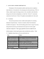
MULTI-FUEL PLATFORM AND TEST PROTOCOLS FOR OVER-THE-ROAD
EVALUATION OF CATALYTIC ENGINE TECHNOLOGY
A Thesis
Presented in Partial Fulfillment of the Requirements for the
Degree of Master of Science
with a
Major in Mechanical Engineering
in the
College of Graduate Studies
University of Idaho
By
Daniel A. Cordon
December 2002
Major Professor: Steven W. Beyerlein, Ph.D.
ii
AUTHORIZATION TO SUBMIT THESIS
This thesis of Daniel A. Cordon, submitted for the degree of Master of Science with a
major in Mechanical Engineering and titled “Multi-Fuel Platform and Test Protocols
for Over-The-Road Evaluation of Catalytic Engine Technology,” has been reviewed
in final form. Permission, as indicated by the signatures and dates given below, is
now granted to submit final copies to the College of Graduate Studies for approval.
Major Professor
Date
Steven W. Beyerlein
Committee
Members
Date
Judi Steciak
Date
David McIlroy
Department
Administrator
Date
Ralph S. Budwig
Discipline’s
College Dean
Date
David E. Thompson
Final Approval and Acceptance by the College of Graduate Studies
Date
Charles R. Hatch
iii
ABSTRACT
Previous research on catalytic igniters and aqueous fueled engines has shown
potential for lowering emissions and increasing engine efficiency over conventional
engine configurations. To quantify these improvements in a vehicle platform, a transit
van has been converted to operate on both gasoline and aqueous fuels, with
changeover possible in less than one hour. Back to back comparisons of baseline
engine and converted engine performance are critical for documenting benefits of
alternative fuel operation on the same vehicle. To facilitate these comparisons this
work developed a test matrix using a steady-state chassis dynamometer
approximating urban and rural driving cycles. Vehicle and test infrastructure created
through this work will support optimization of a broad range of alternative vehicles.
iv
ACKNOWLEDGEMENTS
During the course of this research I had the honor of participating in the Idaho
Engineering Works (IEW) as a mentor for the Capstone Design course. Dr. Edwin
Odom has helped create a graduate experience that has helped me grow personally
and academically greater than any other single educational experience. This
experience formed the basis for a peer-reviewed paper that was delivered at the
2002 Frontiers in Education Conference. I would like to express my gratitude to all
the IEW mentors I have worked and who have inspired me over the last three years.
I would be remiss if I did not thank my major professor, Dr. Steven Beyerlein.
With countless other demands, Steve has always made time to enhance my
graduate experience by jointly writing papers, attending conferences, and
participating in workshops. He has guided both my personal and professional
growth. Steve is an exceptional educator, and has helped seat that passion in me
by creating opportunities for me to teach others.
Throughout this research I have been privileged to work with several fine
organizations. With help from the National Institute for Advanced Transportation
Technology (NIATT), I was able to conduct my research in an environment with
quality instrumentation and facilities. The Idaho Department of Transportation (ITD)
provided the necessary funds to purchase hardware used in the vehicle conversion.
Valley Transit of Lewiston, ID has graciously loaned one of their transit vans as our
test platform, which will one day be added back to their fleet. None of this research
would be possible without the inventions and support of Automotive Resources Inc.
(ARI), providing means for a reliable catalytic ignition source.
v
TABLE OF CONTENTS
AUTHORIZATION TO SUBMIT THESIS .....................................................................................................II
ABSTRACT ....................................................................................................................................................... III
ACKNOWLEDGEMENTS .............................................................................................................................. IV
TABLE OF CONTENTS ....................................................................................................................................V
LIST OF FIGURES..........................................................................................................................................VII
LIST OF TABLES............................................................................................................................................. IX
1
2
3
INTRODUCTION.......................................................................................................................................1
1.1
BENEFITS OF AQUEOUS FUEL COMBUSTION.........................................................................................1
1.2
CATALYTIC IGNITER TECHNOLOGY......................................................................................................2
1.3
DEMONSTRATION VEHICLE DEVELOPMENT .........................................................................................4
1.4
VEHICLE TESTING CAPABILITIES .........................................................................................................4
VEHICLE CONVERSION ........................................................................................................................6
2.1
ENGINE MODIFICATIONS ......................................................................................................................6
2.2
FUEL HANDLING SYSTEM ....................................................................................................................9
2.3
FUEL INJECTION SYSTEM ...................................................................................................................11
2.4
IGNITION SYSTEM ..............................................................................................................................22
2.5
FUEL CHANGEOVER ...........................................................................................................................26
TEST EQUIPMENT.................................................................................................................................30
3.1
CHASSIS DYNAMOMETER ...................................................................................................................30
3.2
FUEL FLOW METER ............................................................................................................................34
3.3
RADAR VEHICLE SPEED DETECTOR ...................................................................................................37
3.4
TEST PROTOCOL .................................................................................................................................39
vi
4
5
EMISSIONS MEASUREMENT .............................................................................................................42
4.1
EMS 5-GAS ANALYZER .....................................................................................................................42
4.2
RADIAN FTIR ....................................................................................................................................44
4.3
BASELINE RESULTS ............................................................................................................................46
CONCLUSIONS AND RECOMMENDATIONS ..................................................................................48
5.1
CONCLUSIONS ....................................................................................................................................48
5.2
RECOMMENDATIONS ..........................................................................................................................49
6
REFERENCES..........................................................................................................................................51
7
APPENDIX................................................................................................................................................52
vii
LIST OF FIGURES
FIGURE 1.0.1 DUAL-FUEL DEMONSTRATION VEHICLE ............................................................................................1
FIGURE 1.4.1 DEMONSTRATION VEHICLE ON THE CHASSIS DYNAMOMETER ...........................................................5
FIGURE 2.0.1 PLAN VIEW OF THE VAN, SHOWING PHYSICAL LOCATION OF COMPONENTS. ......................................7
FIGURE 2.1.1 COMPARISON OF PISTON RING DESIGN ..............................................................................................8
FIGURE 2.1.2 SERPENTINE BELT ROUTING – ORIGINAL ON LEFT, MODIFIED ON RIGHT ............................................9
FIGURE 2.3.1 THREE-DIMENSIONAL VIEW OF FUEL MAP .......................................................................................13
FIGURE 2.3.2 FUEL MAP FOR THE VAN DISPLAYED AS A LOOKUP TABLE ..............................................................13
FIGURE 2.3.3 DIGITAL DISPLAY OF ECM SENSOR VALUES ...................................................................................15
FIGURE 2.3.4 IDEAL SENSOR OUTPUT OF TRADITIONAL OXYGEN SENSOR .............................................................16
FIGURE 2.3.5 A TWO-DIMENSIONAL SLICE OF THE FUEL MAP ...............................................................................17
FIGURE 2.3.6 A 2D FUEL MAP WITH A RANGE OF VALUES SELECTED ...................................................................18
FIGURE 2.3.7 INTERNALS OF THE AEROMOTIVE INC. SERIES A1000 FUEL PUMP ..................................................20
FIGURE 2.3.8 DIAGRAM OF THE INTERNAL WORKING OF THE MSD INJECTORS ....................................................21
FIGURE 2.3.9 AEROMOTIVE INC. FUEL PRESSURE REGULATOR .............................................................................22
FIGURE 2.4.1 IGNITOR IGNITION SYSTEM INSTALLED IN A FORD POINTS DISTRIBUTOR.........................................23
FIGURE 2.4.2 CUTAWAY VIEW OF A CATALYTIC IGNITER .....................................................................................24
FIGURE 2.5.1 VALVE POSITIONS FOR CHANGING BETWEEN FUELS ........................................................................27
FIGURE 2.5.2 ACCESS TO THE ENGINE THROUGH THE INTERIOR ENGINE COVER ...................................................29
FIGURE 2.5.3 BALLAST RESISTOR PROVIDING POWER TO THE IGNITION COIL .......................................................29
FIGURE 3.1.1 SCHEMATIC OF CHASSIS DYNAMOMETER COMPONENTS..................................................................31
FIGURE 3.1.2 HAND-HELD CONTROLLER FOR REMOTE DYNAMOMETER INTERFACE .............................................32
FIGURE 3.1.3 CLOSE-UP OF HAND-HELD DISPLAY ................................................................................................32
FIGURE 3.1.4 CORRECT REAR TIRE POSITION FOR CHASSIS DYNAMOMETER .........................................................33
FIGURE 3.1.5 LOCKING STRAPS USED TO HOLD VEHICLE IN PLACE .......................................................................33
FIGURE 3.2.1 MAX FUEL METERING SYSTEM INSTALLED IN THE VAN .................................................................34
FIGURE 3.2.2 REMOTE RETURN LINE CONNECTION ...............................................................................................35
FIGURE 3.2.3 REMOTE PRESSURE LINE CONNECTION ............................................................................................36
viii
FIGURE 3.2.4 DISPLAY UNIT OF THE FUEL METERING SYSTEM ..............................................................................37
FIGURE 3.3.1 VEHICLE SPEED DATA ACQUISITION ................................................................................................38
FIGURE 3.3.2 DEFINING THE OFFSET ANGLE FOR VEHICLE SPEED CORRECTION ....................................................38
FIGURE 3.4.1 FTP URBAN DRIVING CYCLE TRACE ...............................................................................................40
FIGURE 3.4.2 HIGHWAY DRIVING CYCLE TRACE ..................................................................................................40
FIGURE 4.1.1 EMS MODEL 5001 5-GAS ANALYZER ..............................................................................................43
FIGURE 4.1.2 EMS 5-GAS SOFTWARE ..................................................................................................................44
FIGURE 4.2.1 RADIAN FTIR WITH 10 CM TEST CELL ............................................................................................45
ix
LIST OF TABLES
TABLE 3.4.1 DESCRIPTION OF 6-MODE POINTS .....................................................................................................40
TABLE 4.3.1 RESULTS OF BASELINE TESTING ON VAN ..........................................................................................46
TABLE 5.1.1 KEY DESIGN ELEMENTS OF VEHICLE CONVERSION ...........................................................................48
1
1
INTRODUCTION
The purpose of this project was to create infrastructure for research on
alternative vehicle performance involving catalytic igniter technology. This resulted
in the dual-fuel van shown in Figure 1.0.1 as well as test protocols involving a
steady-state dynamometer that can be used to rigorously evaluate vehicle
performance under different operating conditions. Future phases of this work will
lead to Federal Test Protocol (FTP) driving cycle tests on gasoline and alternative
fuels. Ultimately, this dual fueled vehicle will be studied in over-the-road tests as
part of a local transit system.
Figure 1.0.1 Dual-fuel demonstration vehicle
1.1
Benefits of Aqueous Fuel Combustion
Ethanol is a renewable fuel that is primarily made from agriculture crops [1].
Currently, blends of 85% ethanol and 15% gasoline - called E85 - are commercially
available [2]. Much is published on the emission benefits of ethanol, and many have
taken advantage of ethanol’s inherent attraction to water by mixing small quantities
2
of water into the fuel [3]. Water in the combustion chamber significantly reduces
flame temperatures, and thus reduces NOx formation. In most cases reported in the
literature, the engine is not capable of cold starting on ethanol and must be started
and warmed on a pilot fuel [4]. These cases are also limited to small amounts of
water, as conventional ignition sources are unable to ignite blends of greater than
15% water. In all studies with spark ignition, significant misfire or non-fire occurs
above 10% water present in the fuel.
The University of Idaho and Automotive Resources Inc. have been working
with Aquanol fueled engines since 1996. Aquanol is a mix of 65% Ethanol and 35%
water by volume. While this mixture has not been optimized, it provides a good
balance between NOx minimization and complete combustion of in-cylinder
hydrocarbons. Aquanol-fueled engines have run on mixtures up to 50% ethanol and
50% water, and shown cold starting capability [5]. The current research effort
included a paper at the Bioenergy 2002 Conference that summarized Aquanolfueled engine modifications, the impact of Aquanol on pollutant formation, and
detection of relevant pollutant species [6].
1.2
Catalytic Igniter Technology
The primary drawback to Aquanol is the difficulty of initiating combustion.
Traditional means of spark ignition are insufficient to initiate flame propagation of
Aquanol-air mixtures [7]. An ignition source using a catalytic reaction in a prechamber provides a high-power torch ignition that has proven successful at igniting
mixtures previously un-ignitable by spark or compression ignition [8]. This ignition
source is elementary in the conversion of an engine to operation on Aquanol.
3
Automotive Resources Inc. (ARI) has held the patent on catalytic ignition in a
pre-chamber since 1990 [9]. Since then ARI has made many improvements in the
robustness and ignition control of the catalytic igniter. They have applied this
technology to improve performance and emissions of rotary engines, two-stroke
engines, and used it to combust unconventional fuels in reciprocating IC engines.
Starting in 1996, the University of Idaho started its first research project with
Aquanol. A Yanmar 3-cylinder direct injection Compression Ignition (CI) engine was
converted to run on Aquanol [10]. Direct diesel injectors were replaced with catalytic
igniters, and a manifold fuel injection system was put in place for fuel delivery. In
this engine, there was no throttle plate, so load was controlled only by the amount of
fuel delivered to the engine. Initial research showed that it was possible to burn high
water content with ethanol in an IC engine using catalytic ignition. Further testing
was done to acquire full brake specific fuel consumption and brake specific
emissions maps on both a stock Yanmar diesel engine and the Yanmar converted to
Aquanol fuel [11]. As expected, the emissions of NOx were reduced significantly,
with slight increases in CO and HC – both of which are easily reduced with exhaust
after treatment. Net indicated thermal efficiency increased from 35% on diesel to
42% on Aquanol [12]. With the addition of an intake air pre-heater, the Yanmar
engine demonstrated cold-start and smooth idle capabilities on a 35% water / 65%
ethanol fuel, and operation over air/fuel ratios between 8:1 and 45:1 [12]. These
results were reported in a Society of Automotive Engineers (SAE) paper that we
prepared parallel to the van modifications described in this thesis.
4
1.3
Demonstration Vehicle Development
Making an engine conversion as part of a demonstration vehicle is a powerful
means of sharing the Aquanol and catalytic ignition technology with the general
public. For those doing engine research, demonstrating this technology in a mobile
vehicle platform allows performance to be evaluated in the context of a well-defined
transportation application.
With the success of the diesel engine conversion described in the previous
section, a separate effort was initiated to explore catalytic igniter performance in
Spark Ignition engines. In 1999 NIATT sponsored a senior design project to convert
a transit van for Aquanol operation. The project produced a vehicle that could be
driven short distances on Aquanol, but which was susceptible to fuel system
corrosion, was not capable of dual fuel operation, and which had poor acceleration
characteristics. The purpose of the work reported here was to produce a stable test
platform that supports fuel-injected operation on either gasoline or Aquanol. Details
about the van conversion completed in conjunction with this work are given in
Chapter 2.
1.4
Vehicle Testing Capabilities
As part of the current project, equipment was acquired and integrated for
measuring fuel consumption and emissions. On-board data acquisition in
conjunction with a precision fuel flow meter and radar vehicle speed sensor
accurately measures road load. The newly installed steady-state chassis
dynamometer provides precision control to simulate vehicle loading. Details on
5
vehicle test protocol developed through this work are given in Chapter 3. Figure
1.4.1 shows the van during testing on the chassis dynamometer.
Figure 1.4.1 Demonstration vehicle on the chassis dynamometer
Emissions measurements are necessary to characterize pollutant formation
and analyze exhaust after-treatment effectiveness. A 5-gas analyzer along with a
newly acquired Fourier Transform Infrared (FTIR) spectrometer is a significant start
to building an engine emission measurement infrastructure at the University of
Idaho. Details on improvements to emissions test equipment through this work are
given in Chapter 4.
6
2
VEHICLE CONVERSION
This chapter describes the design of several interacting systems used in the
conversion of a 1985 Ford Extended Van to function on multiple fuels. This was
originally a carbureted engine that was converted to fuel injection for both gasoline
and Aquanol. Not all of the changes made to the vehicle are necessary for
conversion, but as a research platform, the diagnostics and detection components
are crucial for data collection. Figure 2.0.1 shows an overall layout of the fuel and
exhaust handling system. Section 2.1 reviews engine modifications needed to
support Aquanol operation. Section 2.2 describes the fuel handling system,
including fuel storage, valving, and purging. Section 2.3 discusses the fuel injection
system, including the operation of the fuel injection computer. Section 2.4 explains
the ignition systems for both spark plugs and catalytic igniters. Section 2.5 outlines
the process for switching between fuels.
2.1
Engine Modifications
Previously, the van was involved in an engine fire that destroyed most of the
engine compartment. The air conditioning system, heating system, wiring, belts and
hoses were completely destroyed. The engine block and heads were damaged, but
salvageable. Because of this history, some of the engine modifications were more
extensive than would be necessary if starting with a different vehicle platform.
Due to the engine fire, the engine was removed and treated to a standard
overhaul. On the lower block, this consisted of line boring the crank journals, truing
the crank, and installing new bearings for the camshaft, crankshaft, and connecting
7
Figure 2.0.1 Plan view of the van, showing physical location of components.
8
rods. The cylinders were bored and honed to 0.030” larger diameter and new
pistons were installed. On the heads, a three-angle valve job was performed, new
valve guides were installed, and the valve seats were ground to match the new valve
seats.
A common modification to all of the Aquanol engines studied at the University
of Idaho is the installation of Total-Seal piston rings. Traditional piston rings use a
gap in the ring to allow for changes in size due to thermal expansion. When running
Aquanol fuel, this gap allows the water-ethanol fuel to leak past the piston and
contaminate the engine oil. Contamination causes oil breakdown that reduces the
effectiveness of the journal bearings and leads to rapid wear and premature failure.
Also, water in the crankcase promotes corrosion of high-tolerance engine
components. Total-Seal piston rings are a gapless design that reduces mixture
blow-by up to 90% [13]. Figure 2.1.1 shows a comparison of conventional and
gapless piston rings. By using these gapless piston rings, water contamination in
the oil has become undetectable.
Figure 2.1.1 Comparison of piston ring design
Due to damage of some of the engine ancillaries and a need for more space
for the modified fuel system, items like the air conditioning and exhaust air injection
9
components were eliminated from the engine and chassis. These belt-driven
accessories were part of a serpentine style configuration, where one belt drives all
the accessories. By eliminating two of the pulleys, a new system had to be
designed. Because only one belt is use, a single belt tensioner is all that is required
to maintain belt performance. With the two pulleys removed, a logical belt routing
that maintaining comparable pulley contact was designed. Figure 2.1.2 shows the
original and modified belt configuration. This required the belt tensioner to tension
the belt in the opposite direction. Modifications were performed to the original
tensioner to allow this design change. Also, the belt was replaced with a shorter
version, measuring 73.5” in circumference, and having 6 cogs.
Figure 2.1.2 Serpentine belt routing – original on left, modified on right
2.2
Fuel Handling System
One of the major systems unique to a flexible-fuel vehicle is fuel handling.
This research platform was designed to keep two different fuels onboard.
Specifically, individual storage for gasoline and Aquanol are installed. Because
gasoline is the predominant fuel used in the US, nearly all fuel system components
10
are designed to be compatible with it. Alcohol fuels are more corrosive than
gasoline, but when combined with water, Aquanol is even more corrosive. Fuel
handling components designed for gasoline are susceptible to rapid corrosion when
used with Aquanol.
The first Aquanol storage tank was made of steel with the interior surface
coated with Teflon. This was intended to act as a barrier against corrosion. After
two years of use, examination of the fuel tank showed the coating had failed, and
particles were clogging the remainder of the fuel system. Also, the fuel pickup and
fuel lines were not Aquanol compatible. Materials compatible with Aquanol are:
polypropylene, stainless steel, hard anodized aluminum, brass, Teflon, and most
synthetic rubbers. The previous Aquanol handling system was removed and
replaced with a pair of polypropylene fuel tanks, with anodized fuel pickups. The two
Aquanol tanks combined have a capacity of 46 gallons, which yields a similar vehicle
range as a 25 gallon tank of gasoline. The flexible fuel lines are Earls Auto-Flex
hose – constructed of HTE synthetic rubber bonded to a braided stainless steel shell
– and use hard-anodized Ano-Tuff hose ends. All the rigid fuel lines and fittings are
made of 304 Stainless steel, with the exception of anodized aluminum pre-filters.
Because of space limitations, only a single fuel injection system will fit on the
engine. Both fuels share a common fuel pump, high-pressure lines, injectors and
regulator. To accommodate this, a set of stainless valves is used to control the flow
path of fuel. In fuel injection systems the fuel tank has two lines. The suction line
goes to the fuel pump where a constant flow and pressure is attained. Any fuel not
used in the engine is returned back to the fuel tank via a return line. Dual fuel tanks
11
are common on large fuel injected vehicles, and tank selector valves are available
that switch both the suction and return lines at once. These are not compatible with
Aquanol. More importantly, using such a valve will allow the fuel enclosed in the
loop between the inlet and return valves to contaminate the other fuel when
switched. The set of fuel selector valves designed for the van consists of a single Tball valve that switches between the two different fuel sources, and a valve body of
three T-valves to handle flow of the return line. All four valves are modular, and
made of 316 Stainless with a Teflon seat. The three valves are joined by ½”
stainless pipe fittings, coated with anti-seize compound to prevent galling
2.3
Fuel Injection System
Two principal design constraints for the fuel system were corrosion resistance
and a wide fuel metering capability. Conscientious material selection provides a
solution to the first constraint. The heating value of Aquanol has 39% the energy of
gasoline (15.9 MJ/kg vs. 41.4 MJ/kg). Even though engines running Aquanol and
catalytic igniters typically show an increase in net indicated thermal efficiency,
Aquanol still requires over two times more fuel than gasoline to maintain comparable
performance. A careful balance of shared components was necessary to ensure
successful operation on both fuels.
The fuel injection system is responsible for precise metering of the fuel
delivered to the engine. Compression Ignition (CI) engines control engine load by
varying only the amount of fuel delivered to the engine, and thus operate over a wide
range of air/fuel ratios. This is the case for diesel engines, and the Yanmar Aquanol
conversion. Spark Ignition (SI) engines control load by throttling – restricting airflow
12
to the engine. Ideally, SI engines will have a constant air/fuel ratio, but the amount
of air/fuel mixture will vary greatly over operating conditions. The job of the fuel
injection system is to meter the fuel flow to maintain a consistent air/fuel ratio. This
is done with a central Electronic Control Module (ECM) that sends and receives
information from various engine components. These components are detailed in this
section.
The brain of any electronic fuel injection system is the ECM. Electronic
injection systems use maps for making decisions for fuel delivery. These maps are
simply look-up tables that are based on engine speed, and a load measurement.
Factory systems use a hard coded set of maps that are not accessible to the end
user. For this research, a programmable ECM was necessary. We chose a Haltec
model E6A. In our configuration the Haltec ECM has two primary inputs, six
secondary inputs, and one controlled output.
The primary inputs to the Haltec ECM are engine speed and the Manifold
Absolute Pressure (MAP) sensor. The fuel map can be viewed as multiple 2D
maps, one 3D map, or as a lookup table with coordinates of engine speed and
pressure. A 3D map for the van is shown in Figure 2.3.1. Manifold pressure is
shown on the x-axis, engine speed is on the y-axis, and the injector output is the zaxis. A portion of the same map in tabular form is shown in Figure 2.3.2. The
resolution of the maps is 500 rpm – 5000 rpm in 500 rpm increments, and 32 points
of intake pressure between 0 and -30 inches of mercury (gage pressure). When
controlling the engine, the ECM reads only these two inputs to identify the output for
the injectors.
13
Figure 2.3.1 Three-dimensional view of fuel map
Figure 2.3.2 Fuel map for the van displayed as a lookup table
The Haltec ECM has multiple output channels, but for this application only
one control output is being used. This output controls the fuel flow by sending a
pulse width modulated signal to the injectors. The pulse width is the value found in
the lookup table, and is the duration of injection in milliseconds per engine cycle.
Other non-control outputs of the ECM are fuel pump power, and all the sensor
readings for data logging. Optional control outputs can control air-idle valves,
ignition systems, automatic transmissions, turbo controllers, and on-off switches.
14
Secondary inputs to the ECM are engine coolant temperature, inlet air
temperature, rate of change in throttle position, battery voltage, starter engaged, and
a measure of oxygen in the exhaust. These inputs act only as modifiers for the
value found in the lookup table, with the exception of the oxygen sensor. Under
normal operating conditions (190°F coolant temp, 60°F air temp, no throttle
movement, and 14V electrical power) these inputs have no effect on fuel delivery.
They only serve to make adjustments for transient response, or changes in mixture
density. The oxygen sensor can be used to provide closed loop feedback to the
ECM about the actual air/fuel ratio run through the engine. When this feature is
enabled, readings from the Oxygen sensor overrule the value in the lookup table, but
the table itself is not modified.
Because the ECM uses manifold pressure and engine speed to estimate
airflow through the engine, changes in intake/exhaust flow, fuel composition, or
internal engine components will require modifying the fuel map. Knowing how to
make changes to the fuel map is critical for maintaining this research platform. All
changes to the ECM are done though a laptop computer running Haltec software.
The ECM is located below the dash in front of the passenger seat, and the laptop
interfaces with the exposed gray plug. A laptop connection is required for changing
fuel maps or performing data logging. Figure 2.3.3 shows the virtual laptop gauge
display used to view current sensor information, and can be customized to show any
of the input or output values. Engine sensors not displayed in graphical form are still
shown as small numeric values in the lower portion of the gauge screen.
15
Figure 2.3.3 Digital display of ECM sensor values
Even if the ECM is not using the oxygen sensor for closed loop control, this
sensor is invaluable for making adjustments to the fuel map. Oxygen sensors –
except for highly specialized wide-band versions – have a response shown in Figure
2.3.4. They can accurately measure if a mixture is rich, stoichiometric, or lean, but
offer little information on the actual air/fuel ratio. Rich mixtures – ones where there
is not enough air to burn all the fuel – show up as just under one volt. Lean mixtures
– ones where there is excess air after all the fuel is consumed – show up as near
zero voltage. A stoichiometric mixture – one where there is just enough air to burn
all the fuel – will register between 400 and 700 mV. When making changes to the
fuel map, the user must use the output from the oxygen sensor to determine if more
or less fuel should be injected at a certain point on the map.
16
Figure 2.3.4 Ideal sensor output of traditional oxygen sensor
Modifying the fuel map in the Halwin software is relatively simple, but
because the software is a beta version, there is no instruction manual available.
Changes to the fuel map are best done in the 2D view with the vehicle running. To
view the fuel map, use the key sequence “Ctrl+F.” Navigation of the fuel maps is on
the right side of the screen. The “settings” box indicates the current highlighted
value. The three buttons below will change the view between the lookup table, 2D
view, or 3D view. When the “Home Lock” button is pressed, the cursor is kept at
whatever point the engine is currently operating at. For modifying the fuel map,
switch to the 2D view and turn the “Home Lock” off. In 2D mode, injection pulse
width is plotted against manifold pressure for a given RPM range. This RPM will be
17
shown in the box in the upper center of the screen. Figure 2.3.5 shows the 2D map
for 500 RPM. The green arrow above a bar indicates that this is the current position
of the running engine.
Figure 2.3.5 A two-dimensional slice of the fuel map
The map values can be changed one point at a time, or by doing multiple
points at once. To select a point either use the mouse to click on a bar, or use the
left/right arrow keys. The selected bar(s) will be displayed in yellow. By default, only
one bar will be selected at a time. To select multiple bars, hold the “Ctrl” key and
use the left/right arrow keys to selection bars to either side. To unselect multiple
bars, hold the “Alt” key and use the left/right arrow keys to reduce the number of
highlighted bars. In Figure 2.3.6 multiple bars have been selected. Fine adjustment
of the highlighted selection is done using the up/down arrow keys. These will
18
change the injector pulse width by 0.016 milliseconds. Using the “page up/page
down” keys offers a courser adjustment that will move 0.080 milliseconds per
keystroke. Very rough adjustments can be made by holding down the “Shift” key
and using either up/down keys to change values by 0.240 milliseconds, or by holding
down the “Ctrl” key and using either up/down keys to adjust the fuel map by 0.480
milliseconds.
Figure 2.3.6 A 2D fuel map with a range of values selected
Aside from the ECM, several other critical components are necessary for fuel
injection. Of key importance are the, intake manifold, fuel pump, fuel injectors, high
pressure lines, and fuel pressure regulator. A carburetor originally metered fuel for
the vans engine. Intake manifold design for a carbureted engine is vastly different
from one designed for fuel injection. Carburetors have a “wet” intake, meaning the
19
air and fuel must flow through the intake together. Because of this, the shortest
possible runners are usually used to minimize fuel precipitation on the intake walls.
Multi-port fuel injectors mount just before the intake valve, so the intake contains
only air. Also, because each injector will receive the same signal it is important that
each cylinder receive the same amount of air. Thus fuel injection intake manifolds
are designed with long, equal length intake runners that help improve volumetric
efficiency, and a plenum to dampen transient throttle inputs. Even though the 351W
engine was originally carbureted, later versions were offered with multi-port fuel
injection. A factory intake and throttle assembly made for a 1989 Ford Van was
installed in the van.
Fuel injection requires fuel pressures between 30 and 60 psi. Fuel flow rates
must also be considered when selecting a pump. At full speed and load the fuel
pump must be capable of over 300 lbf/hour of Aquanol at 40 psi. Another major
consideration for the fuel pump is corrosion. Bosch is the only manufacturer that
made a high pressure automotive fuel pump fully compatible with Aquanol.
Unfortunately due to low demand, that pump has been discontinued. Aeromotive
Inc. makes a high quality, high flow pump that is mostly compatible. Most of the
internals are stainless, brass, copper, and bronze, but the housing is aluminum.
Figure 2.3.7 shows a cut-away view of the A1000 series pump, which is capable of
450 lbf/hour at 45 psi. One feature of this pump is that it can be disassembled for
inspection or maintenance. When setup for Aquanol use, if the van is to sit idle for
more than a month, it is recommended that the fuel loop be purged with gasoline.
20
Figure 2.3.7 Internals of the Aeromotive Inc. series A1000 fuel pump
Fuel injectors are simply inductance-activated solenoids with a needle and
seat to control fuel flow. Since the engine has eight injectors, each injector must be
capable of nearly 40 lbf/hour. MSD makes a series of injectors that are fully
stainless where in contact with the fuel. A cutaway view of these injectors is shown
in Figure 2.3.8. Flow ratings were given at 35 psi, and injectors with a max flow rate
of 38 lbf/hour were selected. Running a fuel pressure of 40 psi provides adequate
flow for peak requirements on Aquanol. Larger injectors are available, but should
NOT be used if dual fuel capability is desired. Having an injector larger than 40
lbf/hour will not be capable of accurately metering low gasoline flows at idle
conditions.
21
Figure 2.3.8 Diagram of the internal working of the MSD injectors
The loop between the fuel pump and regulator must be capable of handling
internal pressures up to 60 psi. Fuel lines of 304 stainless ½” OD and 0.035” wall
are used for the rigid tubing, but because of engine motion, flexible lines are
required in several places. Earls Auto-Flex hose with Ano-Tuff hose ends are
Aquanol compatible, and rated to 250 psi. All fuel fittings on the van are AN style,
which is a flared seal design. The fuel rail – directly responsible for delivering fuel to
the injectors – is custom made of 304 stainless mated with AN –8 fittings.
The fuel pressure regulator is mounted just downstream of the injectors. It
controls a valve that keeps the upstream pressure at a constant value, regardless of
changes in the fuel pump or change in flow of the injectors. It is important to match
flow capabilities of the regulator and fuel pump, as a “too small” valve will not be
able to keep pressures down, and a “too large” valve will not have fine enough
adjustment for low flows. Aeromotive Inc. makes a stainless and aluminum regulator
22
that is matched to the previously mentioned fuel pump. The A1000 series regulator
is shown in Figure 2.3.9. It features dual inlets, which is important for engines with
more than four injectors. At high fuel demand, local pressure in the rail can change
as much as 1 psi at each injector. With eight injectors, this would lead to a
difference of 8 psi between the first and last injector. By having dual inputs, two
separate lines of four injectors can be used to minimize pressure drop along the rail.
The screw on top is for adjusting rail pressure, and the brass barb on the side
regulates rail pressure in reference to manifold pressure.
Figure 2.3.9 Aeromotive Inc. fuel pressure regulator
2.4
Ignition System
The Haltec E6A has the capability to control spark timing in the ECM. New
Ford 351W engines have distributors designed to work with ECM spark control.
However, after many attempts and modifications the two units were never able to
work together properly. Ignition phasing was inconsistent, and spark timing was
erratic.
23
A stand-alone ignition system has many benefits in a dual-fuel application.
Disabling the ignition as an ECM output can cause reliability problems, and the
added complexity of ECM spark control is unnecessary in this application. A standalone electronic ignition was installed in the van. Made by Pertronix and called the
Ignitor, this system uses an early model point-style distributor, an electronic pickup,
and an ignition amplifier in place of the original points and condenser. This route
provided both ignition robustness, and the proper signal for the ECM. The unit used
in the van is shown in Figure 2.4.1.
Figure 2.4.1 Ignitor ignition system installed in a Ford points distributor
When operating on gasoline, the van uses the above ignition system to create
a spark in the combustion chamber. This spark is delivered by the spark plugs.
Spark plugs come in many different heat ranges for various applications. The heat
range refers to the plugs ability to transfer heat away from the electrode. Typically,
engines with lower combustion temperatures require hotter plugs to maintain plug
life, while the inverse is also true. If a plugs heat range is too low carbon will build
24
up on the electrode and create an alternate non-sparking path for the electricity. If
the selected heat range is too high, the plug can get too hot and cause material
failure. Because of all the modifications to the van, the correct plug heat range was
unknown. Longevity testing has shown that an NGK heat range of 4, an Autolite
heat range of 6, or other brand equivalent are the correct heat range for this
application. This is one of the hottest heat ranges available.
Gasoline has over 2.5 times more energy than Aquanol, yet Aquanol requires
a stronger ignition source. Traditional spark plugs will not ignite, or initiate flame
propagation of an Aquanol-air mixture. Thus, catalytic igniters are a crucial part of
the Aquanol conversion. These operate using a heated catalyst in a pre-chamber
located adjacent to the main chamber. A cut-away of a catalytic igniter is shown in
Figure 2.4.2. For this conversion, each spark plug is replaced with one catalytic
igniter. The four stages of catalytic ignition are: 1) Fuel decomposition on the
catalyst during compression, 2) accumulation of decomposition products and
radicals in rear of pre-chamber, 3) compression ignition of remaining mixture in the
pre-chamber, 4) rapid torch ignition of the main chamber. Using catalytic igniters
changes the engine to a Homogeneous Charge Compression Ignition (HCCI)
configuration.
Figure 2.4.2 Cutaway view of a catalytic igniter
25
Controlling ignition timing is probably the most crucial aspect of catalytic
igniter design. Where spark plugs receive a precisely timed input to initiate
combustion, catalytic igniters operate on their own. In previous designs, ignition was
controlled by changing the position of the catalyst in the pre-chamber. The closer
the catalyst resides to the combustion chamber, the earlier ignition would occur.
Typically ignition timing should advance with engine speed, and retard with load so
that peak pressure is reached at or shortly after TDC. In this system, the opposite
was true.
The van features a new generation of catalytic igniter. Location of the
catalyst is fixed at the leading edge, but the inner pre-chamber diameter is much
smaller. Having the catalyst closer coupled to the pre-chamber wall allows for
differences in mass to change ignition timing. Under part throttle conditions, there is
less mass in the cylinder than under high load conditions. Under high load
conditions, the higher mass causes a slight quenching effect with the wall that
delays ignition timing – a desirable outcome for high load conditions. This new
generation of catalytic igniter is also able to maintain the crank angle of peak
pressures over a wide RPM range.
Setup of catalytic igniters requires measuring in-cylinder pressure to verify
ignition timing. To do this, one combustion chamber was machined for a
piezoelectric pressure transducer to measure cylinder pressure. By looking at the
pressure trace on an oscilloscope, ignition timing can be deduced. Figure 2.4.3
shows pressure trace trends for ignition timing. Ignition timing is adjusted until a
pressure trace like the “MBT timing” is achieved.
26
Figure 2.4.3 Pressure vs. crank angle for varied ignition timing
2.5
Fuel Changeover
Switching between fuels is a quick multi-step process. The Figures 2.5.1 a –
e follow an example of switching from gasoline to Aquanol. 1) With the vehicle
turned off, switch the suction valve to the fuel of choice. 2) Hook up a purge line to
the purge valve of the chosen fuel and verify the valve is directing fuel out the purge
line. 3) Switch the center return line valve to direct flow to the chosen fuels purge
valve. 4) With the end of the purge line in a purge container, power the fuel pump
via the remote power connection. 5) Run the pump until all the previous fuel has
been flushed. When switching from gasoline, the fuel will be amber colored at first,
then become clear when flushed with Aquanol. 6) Remove power from the pump
and switch the purge valve to flow to the fuel tank return line. 7) To prevent cross
contamination due to leakage, switch the un-used fuel tank purge valve to exit the
27
purge side. At this point, the fuel system is switched to the desired fuel. When
finished, all the handles on the return valve body should face the same direction.
a) Suction valve set for gasoline
b) Suction valve set for Aquanol
c) Return valve positions for gasoline
d) Purging with Aquanol
e) Return valve positions for Aquanol
Figure 2.5.1 Valve positions for changing between fuels
28
Because of the different needs in fuel quantity, the fuel map must be changed
when switching fuels. To do this, connect a laptop computer to the Haltec ECM
through the serial port. Turn the ignition on so that the ECM receives power, but do
not start the engine. Open the Halwin software and establish a connection with the
ECM. A copy of the current fuel map should be saved before overwriting it. To do
this, click “Save all Maps” under the “File” menu and enter a name for the maps. A
good choice would be something like “[fuel type], [date].” Next, select “Load all
Maps” under the “File” menu and select the map for the desired fuel. At this point
the fuel maps will automatically be uploaded to the ECM. Quit the Halwin software
and turn the ignition switch off.
The last part of changing between fuels is to change ignition systems. When
changing from spark ignition (gasoline) to catalytic ignition (Aquanol), start by
removing the interior engine cover – located just in front of and between the driver
and passenger seats. Figure 2.5.2 shows the engine with this cover removed.
Detach the spark plug wires from the spark plugs, and remove the spark plugs.
Install the catalytic igniters by threading them in to the spark plug holes, and
attaching the power wire lead to each end. Reconnect the igniter power feed wire
next to the fuse block mounted to the center console. Reinstall the interior engine
cover. With the hood open, remove the distributor cap with the ignition wires still
attached. Remove the power to the ignition coil by disconnecting the terminal on the
ballast resistor. The ballast resistor is centered above the engine on the firewall,
and shown in Figure 2.5.3. Changing from Aquanol to gasoline is just the reverse of
above. Even when the spark ignition system is not being used, do not remove the
29
distributor from the engine. The ECM still reads the tachometer signal from the
distributor, and the oil pump will not function when the distributor is removed.
Figure 2.5.2 Access to the engine through the interior engine cover
Figure 2.5.3 Ballast resistor providing power to the ignition coil
30
3
TEST EQUIPMENT
This chapter outlines the equipment used for vehicle testing at the University
of Idaho. Fundamental to this research is the recently installed chassis
dynamometer in Martin Laboratory. This allows steady state load simulation of the
vehicle in a controlled environment. Accurate road-load simulation requires precise
data on vehicle speed and load for actual driving conditions. A radar speed sensor
is used in conjunction with information from the Haltec ECU to measure and
duplicate these parameters. Section 3.1 discusses operation and setup of the
chassis dynamometer. Section 3.2 explains hookup and function of remote fuel
measurement system. Section 3.3 describes data collection using a Doppler radar
speed sensor. Section 3.4 details the equipment used for vehicle testing and
outlines the protocol for performing vehicle tests.
3.1
Chassis Dynamometer
A rolling chassis dynamometer has been installed in one of the high bays of
the J. Marin Laboratory. The SuperFlow SF-602 is an integrated system of
dynamometers, data acquisition, and load control. A schematic of this system is
shown in Figure 3.1.1. Two large rollers, 36” in diameter and 96” wide, are each
directly connected to a 550 HP water-brake dynamometer. A precision load cell is
used to measure torque on the dynamometer, and optical sensors measure wheelspeed. A high pressure, high flow pump pulls cool water from a storage tank and
sends it to a control valve. Changing water flow to the dynamometer is how load is
controlled. The control valve is remotely operated by inputs from the hand-held
controller, processed by a computer in the external digital readout. Hot water
31
ejected from the dynamometers flows through a set of valves – used to balance the
two dynamometers – then in to a vented tank. From here, a high flow, low pressure
pump pushed the hot water through a heat exchanger, then back in to the storage
tank.
Figure 3.1.1 Schematic of chassis dynamometer components
Load control of the chassis dynamometer can be either open or closed loop.
The hand-held controller shown in Figure 3.1.2 is used to set the load. Current
performance information is displayed in the center, with menu/control options around
the perimeter. A detailed view of the hand-held display is given in Figure 3.1.3.
When operating in open loop control, the hand-held controller allows the user to
manually open or close the control valve. There are both fine and course
32
adjustments. Using feedback from various sensors, control can also be set to
maintain a constant vehicle speed, engine speed, HP, or torque value. In this mode,
the hand-held controller allows input of the desired parameter value, and a computer
within the external digital display automatically adjusts the control valve to maintain
the specified value.
Figure 3.1.2 Hand-held controller for remote dynamometer interface
Figure 3.1.3 Close-up of hand-held display
The following is an abbreviated set of steps used to setup the vehicle for
chassis dynamometer testing. For a full list, refer to the appendix. Lock the rollers
33
and back the vehicle on to the center of the rollers. Attach the rear safety chain and
allow the vehicle to roll forward. With the chain taunt, the tires should be forward of
the roller centerline as pictures in Figure 3.1.4. Make sure that the front tires are
centered between the tie-down rails, and lock them in place with straps as shown in
Figure 3.1.5. Attach all sensors that will be used in the test. Connect the exhaust
plume to the vehicle exhaust system. At this point, the vehicle is ready for testing.
Figure 3.1.4 Correct rear tire position for chassis dynamometer
Figure 3.1.5 Locking straps used to hold vehicle in place
34
3.2
Fuel Flow Meter
Fuel consumption is an important parameter when comparing various
modifications to a vehicle. To determine fuel consumption, a positive displacement
fuel measurement system is used. A MAX Machinery 710 series fuel flow meter was
purchased because of its compatibility with Aquanol and gasoline, and the ability to
measure both the feed and return lines that are used with fuel injected engines. This
system consists of a remote fuel tank, a fuel metering box, and a remote display.
These can be seen installed in the van in Figure 3.2.1.
Figure 3.2.1 MAX fuel metering system installed in the van
When used, this system replaces the tasks of the fuel tank and fuel pump.
To connect the fuel system to the van, start by removing the fuel pump relay. This is
located on the passenger side firewall. Remove the interior engine cover and
disconnect the flexible fuel line from the bottom of the fuel pressure regulator. Install
the shorter of the two fuel meter lines to the bottom of the regulator and plug the
original return line as seen in Figure 3.2.2. Open the hood and remove the lower
35
connection to the fuel T fitting. Attach the longer of the two fuel meter lines to the T
fitting inlet and plug the original line as shown in Figure 3.2.3. Both plugs are size
AN –8. Route the two fuel lines to the fuel meter, making sure they are not near the
exhaust, or moving engine components. Lastly, the fuel cart requires a 12V source
for power. A remote battery near the fuel meter needs to be connected to the main
vehicle battery with a minimum of 8-gage wire. Connect the fuel meter to the
battery. Plug in the lines to the engine and remote fuel tank in to the fuel meter,
switch the meter on, set the fuel pressure by turning the blue knob. Because the
fuel pressure regulator is still installed in the system, the meter pressure will never
pressurize above the regulated pressure. Check for leaks at all the fittings, then reinstall the engine cover.
Figure 3.2.2 Remote return line connection
36
Figure 3.2.3 Remote pressure line connection
With the fuel connections in place, the fuel system is ready for use. The
display is the primary feedback for the user, and has several functions. The display
unit is pictured in Figure 3.2.4. Because the meter uses positive displacement
sensors it is actually measuring a volume flow rate, yet the top panel of the display
reports a mass flow rate [kg/hr]. Specific gravity as a function of temperature is
required for a precision measurement. The knob below the temperature display
switches this function between four fuels. Setting #2 is for gasoline, and setting #4
is for Aquanol.
37
Figure 3.2.4 Display unit of the fuel metering system
3.3
Radar Vehicle Speed Detector
In preparation for emissions measurement over a Federal Test Protocol (FTP)
driving cycle extensive vehicle roll-down data is required. In a roll-down test a
vehicle is driven to 60 mph on a flat road, then the transmission is put in neutral and
the vehicle coasts until it reaches 20 mph. This is done several times on the same
road, and runs in opposite directions are averaged. Data on speed vs. time is
gathered so that roll-down characteristics can be mimicked on the chassis
dynamometer.
To get data vs. speed, a non-contact Radar Doppler Vehicle Speed Sensor
and IOtech mobile data acquisition system were purchased. They connect to a
laptop computer as shown in Figure 3.3.1, and allow data collection as high as 100
38
points per second. The sensor outputs a frequency proportional to vehicle speed.
This must be corrected using the equation
Vehicle _ speed =
sensor _ output[ Hz ]
* cos(θ )
Hz
211.598
mph
where θ is the offset angle as shown in Figure 3.3.2. Because the offset angle has a
mild effect in calculating vehicle speed, this angle should be measured to within 1-2°.
When mounted on a vehicle, the optimal angle for this sensor is 30°.
Figure 3.3.1 Vehicle speed data acquisition
Figure 3.3.2 Defining the offset angle for vehicle speed correction
39
3.4
Test Protocol
A primary thrust of this research was to create a test protocol that would allow
local testing of the vehicle that would mimic the FTP driving cycles. This would allow
preliminary testing and comparisons of fuel economy and emissions between the
two fuels. Approximating a FTP driving cycle locally allows the fuel mapping and
exhaust after treatment to be evaluated and modified for best possible vehicle
emissions and performance.
The FTP driving cycle is a speed-time trace that a vehicle must follow while a
transient chassis dynamometer mimics road power requirements. The FTP-72 trace
imitates city driving, and is shown in Figure 3.4.1, while the Highway Fuel Economy
Test (HWFET) is shown in Figure 3.4.2. With no transient dynamometer existing in
the Northwest, an approximation using the steady-state chassis dynamometer must
be used. A six-mode test was created that will collect data at four steady state
points and two mock-acceleration points. These are shown in Table 3.4.1.
Emissions will be reported in percent and parts-per-million (ppm) depending on the
species, and fuel consumption reported in both kg/hour and miles per gallon (mpg).
To estimate driving cycle performance, weighting factors are applied to each data
point representing percent time of each point in the FTP-72 and HWFET driving
cycles. Other countries still use weighted steady-state modal tests for new vehicle
certification. Until 1996, Japan used a six-mode certification for vehicles carrying
over 10 passengers, which has been updated to a 10-mode test [14]. Emissions in
their six-mode test are expressed in percent composition, but their loading
parameters and weighting factors differ significantly from the above protocol.
40
Figure 3.4.1 FTP Urban driving cycle trace
Figure 3.4.2 Highway driving cycle trace
Mode
1
2
3
4
5
6
Speed
Idle
25 mph
20 mph
45 mph
40 mph
60 mph
Table 3.4.1 Description of 6-mode points
Load
--Road Load
50% throttle
Road Load
50% throttle
Road Load
Weighting
0.05
0.35
0.15
0.25
0.10
0.10
41
When preparing for chassis dynamometer testing, data must be gathered
about road load for three points. The Haltec Halwin software and radar speed
sensor are used for initial data collection. As with roll-down testing, the data must be
collected on a flat, straight road, and should be verified multiple times in each
direction. Before measuring road load, the vehicle speedometer must first be
calibrated. Use the radar speed sensor to determine the vehicles speedometer
reading for each speed. This will vary with tire size, and slightly with tire pressure
and wear. To measure road load, drive the vehicle at the desired steady-state
speed and use Halwin software to collect data on the engine speed, percent throttle,
manifold pressure, engine and air temperature, and injector duty cycle.
The data gathered on the above road testing will be used to re-create the
same conditions on the chassis dynamometer. Once the vehicle is set up on the
chassis dynamometer, do some light driving to bring the engine to operating
temperature. It is easiest to use the “hold vehicle speed” feature on the hand-held
controller. Set the desired vehicle speed on the controller, and move the throttle to
the recorded setting. Due to variations in barometric pressure, throttle angle alone
will not guarantee simulation of the road load. It does give a good starting point.
Once the dynamometer control has stabilized, adjust the throttle slightly to achieve
the desired manifold pressure associated with the given road load speed. Verify that
the injector duty cycle matches the road load data, then collect data on emissions,
fuel consumption, engine and air temperature, and vehicle speed. In between
simulating points it may be necessary to remove the dynamometer load to allow the
engine to cool down. This is especially true for the high load points.
42
4
EMISSIONS MEASUREMENT
This chapter contains information about emissions testing equipment used to
detect chemical species typically found in vehicle exhaust. Of particular interest in
vehicle exhaust is emissions of Carbon Monoxide (CO), Carbon Dioxide (CO2),
Oxides of Nitrogen (NOx), and Hydrocarbons (HC). Currently a 5-gas analyzer is
used to measure these species, but a Fourier Transform Infrared Spectrometer
(FTIR) is being modified to provide detailed breakdowns of exhaust compositions.
Section 4.1 describes use of the 5-gas analyzer. Section 4.2 discusses the
usefulness of a FTIR as a tool for detailed exhaust analysis. Section 4.3 reports
preliminary results on the van while running gasoline without a catalytic converter.
4.1
EMS 5-gas Analyzer
The EMS model 5001 5-gas analyzer is a flow-through meter with individual
sensors for specific species, shown in Figure 4.1.1. Small percentages of the
exhaust stream are pulled through a probe placed in the exhaust system, and are
assumed to be representative of the total mixture in the exhaust stream. Inside
reside sensors for oxygen, NOx, CO, CO2, and unburned hydrocarbons. The unit
has its own pump, and separate exhaust lines for water and exhaust products.
Power for the 5-gas is provided by a cigarette lighter socket, or using alligator
clamps with an adapter. When connected, the 5-gas analyzer automatically starts a
warm up process, which may take up to 10 minutes depending on ambient
temperature. While in the warm up mode. Dashed lines will flash in the displays.
Once warm, the 5-gas automatically goes in to sample mode.
43
Figure 4.1.1 EMS model 5001 5-gas analyzer
Being a flow-through devise, transient response with the 5-gas analyzer is
relatively slow, and depends greatly on the length of hose between the unit and the
emission source. Even when in steady state operation, emissions from an IC engine
will fluctuate. To help data collection, the 5-gas can be connected to a computer for
data logging. The EMS software, shown in Figure 4.1.2, has a recording option
called “Road Test.” In this mode the unit continuously samples, but data is not
recorded until the space bar is pressed. When pressed, the software records and
averages emissions over a 10 second period. Multiple road tests can be done in a
given test session.
44
Figure 4.1.2 EMS 5-gas software
Constant upkeep of the 5-gas is required to maintain accuracy. The unit
should be checked against a calibration gas before any testing, but typically requires
calibration every few months. Because of decay of electrochemical sensors, the 5gas should be checked annually by a certified repair center. Sensors require
replacement every 2 and 5 years depending on the sensor and severity of use. The
5-gas analyzer provides highly accurate data on NOx, O2, and CO, but is less exact
in reporting CO2 and HC’s.
4.2
Radian FTIR
Though currently unregulated, aldehydes are a significant exhaust product of
alcohol-derived fuels. Methanol fuel tends to primarily produce formaldehyde, while
ethanol forms acetaldehyde. Both species show up as part of hydrocarbon
emissions, but demonstrate higher reactivity in photochemical smog formation than
45
other hydrocarbons. To measure aldehyde emissions, exhaust gases must be
analyzed in much greater detail.
A FTIR is a flow-through devise like the 5-gas analyzer, but the method of
detection differs greatly. The Radian FTIR is pictured in Figure 4.2.1. A heated
pump diverts some of the exhaust stream through insulated lines that help prevent
water precipitation. This mixture flows in to a chamber where it is penetrated by a
laser. Photo detectors pick up the intensity spectrum over a frequency range. The
frequency band excited, and magnitude thereof correspond to a species and
concentration. Several specialized computer programs and significant verification
were necessary to set the machine up.
Figure 4.2.1 Radian FTIR with 10 cm test cell
Testing with the FTIR requires the sensors to be cooled with liquid nitrogen,
and the whole enclosure to be purged with gaseous nitrogen. Background sampling
46
and setup can take as much time as an hour. Because the test section on the FTIR
has significant volume, it is difficult to get good transient response, though this same
volume helps damp out small fluctuations in exhaust concentration. Once set up,
taking a data point will take between 3 and 15 minutes, depending on the resolution
required. The FTIR is too cumbersome to use for casual testing, but is invaluable
when comprehensive exhaust analysis is required.
4.3
Baseline Results
Using the test protocol outlined in chapter 3 and the 5-gas analyzer described
above, preliminary testing was done to verify all of the systems would function as
planned. Road load data was collected and a six-mode simulation was performed
using the steady state chassis dynamometer. This testing was done on a nonoptimized fuel map without a catalytic converter, but demonstrated local capability to
provide repeatable data about emissions and fuel consumption in a controlled
environment. Results are shown in Table 4.3.1.
Mode
1
2
3
4
5
6
Weighted
Speed [mph]
15
25
20
45
40
60
Load
Idle
Road
50%
Road
50%
Road
Weight factor
0.05
0.35
0.15
0.25
0.10
0.10
CO2 [%}
12.7
12.8
8.5
11.6
10.7
13.5
11.71
CO [%]
0.07
2.44
9.4
4.59
6.13
1.5
4.18
NOx [ppm]
174
1150
201
1024
640
2321
993.45
HC [ppm]
152
359
300
327
254
262
311.60
Fuel rate
2.45
6.44
27.4
13.5
30.13
16.7
14.54
Fuel use
18.21
11.54
2.17
9.91
3.95
10.68
9.22
Table 4.3.1 Results of baseline testing on van
47
Based on these preliminary results, it is clear that the fuel map provided
inconsistent air/fuel metering at the time of testing. Mode 3 is high load, yet one of
the lower points for NOx emissions. This would be abnormal from a fine tuned
engine, but the increase in CO in that mode points towards a rich mixture.
Conversely, Mode 6 appears to be lean with very high NOx, and low CO emissions.
Weighted fuel consumption falls between observed fuel economy for the van of 7
mpg (city), and 11.5 mpg (hwy).
48
5
CONCLUSIONS AND RECOMMENDATIONS
Development of this demonstration platform and test protocol completes a
major milestone in the exploration of an emerging and exciting technology. Still in its
infancy, catalytic engine technology promises to be a renewable, clean alternative
energy source that reduces dependence on fossil fuels. Section 5.1 summarizes
conclusions from this work. Section 5.2 supplies recommendations for future work.
5.1
Conclusions
This work has produced a robust, reliable vehicle platform for evaluating
alternative fuel performance. A transit van owned by Valley Transit has been
modified for this purpose. The new fuel handling system shows no sign of corrosion,
and gasoline fuel economy and emissions are far improved over the original
carbureted configuration. Data logging capabilities have been added that will
facilitate analysis of vehicle performance under controlled test conditions. Table
5.1.1 highlights design features of the converted transit van.
Item
Feature
Programmable fuel injection
Manual fuel switching valves
TotalSeal piston rings
On-board data logging
Fuel system components
Stand-alone ignition system
New gen. catalytic igniter
Combustion sample port
Dual-fuel design
Allows control of fuel metering for various fuels
Permits purging to prevent fuel contamination
Reduces blow-by and eliminates oil-fuel contact
Tracks and records ECM input and output values
Resistant to highly corrosive fuels
Provides reliable, easily disabled ignition source
Supports combustion of alternative fuels
Collects in-cylinder pressure data
Switches fuel configuration in less than one hour
Table 5.1.1 Key design elements of vehicle conversion
49
The vehicle test protocol developed through this work effectively utilizes
equipment and facilities available at the University of Idaho. This system accurately
simulates vehicle road load conditions, and provides a means of evaluating small
design changes. Infrastructure assembled as part of this work is not limited to the
transit van, but can – and should – be used for assessing effectiveness of
modifications to a variety of research vehicles.
Our current emission detection equipment represents an adequate balance of
usability and complexity. The 5-gas analyzer is a powerful tool for sampling exhaust
emissions. The ability to use this equipment for either mobile or stationary data
collection is unmatched by other detectors.
5.2
Recommendations
The work described here represents a first pass at developing a vehicle test
platform and protocol for fuel consumption and exhaust emission measurement.
Both the protocol and vehicle platform have been tested, but further development of
each promise to enhance vehicle test capabilities at the University of Idaho.
Recommendations concerning emission detection, and future vehicle modifications
are detailed in this section.
The 5-gas analyzer provides excellent screening of emissions, but does not
produce EPA certified results. The FTIR is a research-grade piece of equipment for
collecting detailed information on exhaust composition that can fill this niche. The
FTIR needs temperature controlled sample lines to preventing exhaust
condensation. Water condensed in the exhaust absorbs aldehydes and results in
50
inaccurate composition detection. Measurement of mass flow in the exhaust is
required to report emission results in standardized units of grams per mile.
Thus far, intermittent vehicle use is the primary reason for component
failures. To best of our knowledge, this has been limited to external components.
At some point, inspection of internal engine parts through an engine teardown
should be undertaken to assess adverse impact of dual fuel use. A regimen of
weekly, or bi-weekly trips would serve to avoid potential problems in the future.
Regular use would also promote public awareness that is an important by-product
on alternative fuel research at the University of Idaho.
A number of platform modifications are necessary to provide passenger
comfort if this vehicle becomes an active element of a local transportation system.
These include a heater for the driver and cabin as well as a defroster system.
Enlarging the cooling system will reduce heat build-up during summer driving and is
likely to provide better thermal management of the engine when the vehicle is on the
dynamometer.
Several additional changes to the van are advisable to improve both function
and appeal. Daily drivability in an alternating climate would be greatly improved if
more ECM control features were enabled. ECM control of the air-idle control valve
would stabilize engine speed during warm-up. Incorporating wide-band oxygen
sensor feedback to the ECM will allow fuel tuning for lean Aquanol mixtures. A
dedicated laptop or PC tablet mounted in the van would serve as a permanent
interface for ECM tuning, provide constant data logging, and potentially offer visual
feedback about engine parameters to transit patrons.
51
6
REFERENCES
1.
Nadkarni, R. A., Guide to ASTM Test Methods for the Analysis of Petroleum
Products and Lubricants, ASTM Publishing, West Conshohocken, PA, 2000
2.
Wyman, C. E., Handbook on Bioethanol, Production and Utilization, National
Renewable Energy Laboratory, NICH Report 24267 (424), 1996.
3.
Lee, W., and Geffers, W., “Engine Performance and Exhaust Emissions
Characteristics of Spark Ignition Engines Burning Methanol and Methanol
Mixtures”, A.I.Ch.E. Symposium Series #165, Vol. 73, 1977.
4.
Jehlik, F., Jones, M., Shepherd, P., Norbeck, J., Johnson, K., McClanahan, M.,
“Developnent of a Low-Emission, Dedicated Ethanol-Fuel Vehicle with ColdStart Distillation System,” SAE Paper 1999-01-0611, 1999.
5.
Morton, A., Genoveva, M., Beyerlein, S., Steciak, J., Cherry, M., “Aqueous
Ethanol-Fueled Catalytic Ignition Engine,” SAE Paper 1999-01-3267, 1999.
6.
Cordon, D., Clarke, E., Beyerlein, S., Steciak, J., Cherry, M., “Comparison of
Water-Ethanol and Gasoline Fuels in an On-Road Test Platform,” Bioenergy
Conference, Paper 2094, 2002.
7.
Cherry, M., Morrisset, R., and Beck, N., “Extending Lean Limit with MassTimed Compression Ignition Using a Plasma Torch,” SAE Paper 921556, 1992.
8.
Gottschalk, Mark A., “Catalytic Ignition Replaces Spark Plugs,” Design News,
May 22, 1995.
9.
Cherry, M., Catalytic-Compression Timed Ignition, US Patent 5 109 817,
December 18, 1990
10.
Morton, A. T., “Homogeneous Charge Combustion of Aqueous Ethanol in a
High Compression Catalytic Engine,” MS Thesis, University of Idaho, 2000.
11.
Clarke, E., “Characterization of Aqueous Ethanol Homogeneous Charge
Catalytic Compression Ignition,” Masters Thesis, University of Idaho, 2001.
12.
Cordon, D., Clarke, E., Beyerlein, S., Steciak, J., Cherry, M., “Catalytic Igniter
to Support Combustion of Ethanol-Water/Air Mixtures in Internal Combustion
Engines,” SAE Paper 02FFL-46, 2002.
13.
Total Seal Inc., “Gapless Technology,” http://www.totalseal.com/gaplesss.html.
14.
DieselNET, “Emission Standards,” http://www.dieselnet.com/standards/cycles.
52
7
APPENDIX
A:
Part Numbers of Modified Components
B:
Haltec ECM Setup Values
C:
MathCAD Fuel Calculations
D:
SuperFlow SF602 Specifications
E:
Chassis Dynamometer Vehicle Setup Instructions
F:
MAX Fuel Meter Manual
G:
EMS 5-gas User Manual