Download masters thesis_final_md_abdul_kader_sagar

i
AUTOMATED ACQUISITION APPROACHES FOR MULTIDIMENSIONAL
MULTIPHOTON MICROSCOPY
By
Md Abdul Kader Sagar
A dissertation submitted in partial fulfillment of
the requirements for the degree of
Masters of Science (Electrical Engineering)
at the
UNIVERSITY OF WISCONSIN-MADISON
2015
ii
Table of contents
Table of contents
ii
Dedication
Acknowledgement
Abstract
Introduction
Microscope automation and instrumentation
Laser wavelength Control
Filter wheel sequencing with Pockels cell
Neutral Density filter control
White balance for white light image acquisition:
Fluorescence lifetime imaging (FLIM) setup
iii
iv
v
1
2
3
4
5
6
7
Lifetime board installation (SPC-150)
Relay circuit
Variable neutral density filter
Next steps
SLIM Curve
Macro language support
Using Segmentation
Comparison of result
9
12
12
14
14
15
15
16
Future Development
17
Conclusion
18
Appendix
19
Laser control with instruction set and controlling class
19
Using Filter sequencing
22
Neutral Density Filter-wheel control
22
White balance code
23
Lifetime acquisition library and flowchart of lifetime imaging
25
Sample macro recorder
28
Installing SLIM Plugin
31
Segmentation of FLIM using Trainable Weka segmentation
32
References
35
iii
Dedication
To my parents, M A Mazid and Kamrun Nahar Jasmin, beloved wife Nafisah Islam, my friends,
my teachers and all who have inspired me to come this far.
iv
Acknowledgements
I am very thankful Kevin Eliceiri, who have inspired me and guided me through every step of my
graduate studies, research and academic work. From the very beginning he has guided me in proper
way, tried his best to find out what suits me best and align my work with my interest. Watching
him work every day and getting guidance from was a big motivation for me in my graduate work.
I am also deeply indebted to all the members in LOCI who made me very comfortable in this new
country and new working environment. I would specially like to thank Ajeet Vivekanandan and
Adib Keikhosravi who have been extraordinarily helpful with my projects from the very
beginning. I would also like to thank Josh Weber whom I have been collaborating with installing
the lifetime system and fine-tuning other systems in lab. Brian Burkel has also been very helpful
for understanding the basics of lifetime imaging system and theory behind it.
I would also like to thanks Professor Dan Negrut who have been kind enough to be my advisor.
Without the inspiration of my parents, I think it would be hard for me to pursue graduate studies
at the beginning. My friends who inspired me to purse this life. I would like thanks them. In
addition, thanks a lot to my beloved wife to be beside me for achieving this challenging task.
v
Abstract
Recent development in laser scanning microscopy relies increasingly on the automation. Important
part of the laser scanning microscopes like laser, galvanometer, photomultiplier tube (PMT), filterare now automated and come with their own instruction set. This automation enables us to do
sequencing in five dimensions. Automated multi parameter imaging enables us to look at sample
with more ways that eventually results in better understanding of the sample. Sequencing with
varying all parameters associated with imaging will enable user to excite different fluorophore in
different wavelength with laser wavelength sequencing and look at their emission at different
wavelength with filter sequencing. In my effort to make multiphoton microscopy automated, I
have developed laser automation, filter automation, white balancing bright-field image. To
improve multi parameter, multidimensional sequencing I have developed filter sequencing.
Fluorescence-lifetime Imaging Microscopy (FLIM) is a technique to understand cellular
metabolism and cancer metastasis. I have installed and optimized a SPC-150 lifetime board in a
multiphoton microscope and tested some standard samples for lifetime measurement, which gave
promising results with standard lifetime samples. To analyze FLIM data, I have contributed on
developing SLIM Plugin that is an open source exponential curve-fitting library for analyzing
FLIM images.
Keywords: Multiphoton Microscopy, FLIM, Curve-fitting, Sequencing, metabolism, Cancer
detection
1
1. Introduction
Multiphoton microscopy has become the technique of choice for imaging live animals and live
tissue. Multiphoton microscopy(MPM) has proved to be very valuable for cancer research for in
vivo studies of metastasis(1,2). Second Harmonic Generation(SHG) microscopy is also widely
used method for looking at live tissue and disease diagnosis(3–6). A typical multiphoton
microscope is composed of a femtosecond laser, a low magnification high-numeric-aperture
objective a wavelength-sensitive dichroic and a detector(7). The scanning system uses a raster
scanning method to raster the excitation beam in the two dimensional field at the full numerical
aperture of other objective. There is an incredible amount of information that can be acquired at
the focus of the multiphoton microscope with proper detectors, filters. Modern microscopy is being
increasingly relying on computer-based automation and most of the parameters, which control the
imaging environment, are now controllable from computer. For example, now the lasers are fully
controllable from external computer via the RS232 port with hyper-terminal. Before computer
based model for laser control, the wavelength was controlled manually with an on-board controller.
With modern laser, they come with their own software suite with external command soft for serial
port. Changing filter is also fully automated with newer filter wheels. Galvanometers-based optical
scanners are now controlled externally from FPGA/Digital signal processor. Galvanometers create
the waveform from the control the raster scanning which sends the laser to the sample. The detector
sends signal to the computer, which recreates the image at that plane. To make look into larger
sample, stages are used which can be translated in X-Y axis. Addition of Z-axis motor gives control
in Z-axis. Combination X-Y stage and Z-axis motor gives us control to image any location in three
dimensions. With the introduction of Bio-Formats(8) library and OME-XML/OME-TIFF it has
been possible to add necessary metadata to the acquired images which can be later stitched by
ImageJ. Stitching made it possible to look at very large sample at once and analyze them to get
more information. These functionalities described above-controlling galvanometers, detecting
reflected photon from photons, controlling the stage in X-Y-Z axis, changing filterwheel, inserting
metadata with X,Y,Z with other imaging parameter information- all these functionalities are
already developed and available in our developed software WiscScan (9).
WiscScan combines all the basic functionalities of laser scanning microscopes. However, more
automation is required to perform advanced imaging like spectral microscopy. Spectral imaging
requires the wavelength to change automatically to excite different fluorophore in their excitation
wavelength, also it requires appropriate filter to look at proper emission wavelength(10). To enable
WiscScan to accomplish spectral imaging, it needs to have full control over laser wavelength and
filterwheel control along with ability to control laser power. I worked on automation of laser
wavelength control and ability to change power of laser through Pockels cell, which control power,
automation of filter during sequencing storing the metadata for enabling stitching.
2
Fluorescence-lifetime Imaging Microscopy (FLIM) is imaging modality that helps to understand
metabolism in cell. As NADH/NAD+ reduction-oxidation pair is crucial for electron transfer in
the mitochondrial electron chain, biochemical estimation of NADH concentration is a useful
method for monitoring cellular metabolism. NADH fluorescence is used for interpret metabolic
activity within the cell(11,12). There are many groups that have shown with quantitative NADH
fluorescence measurement significant difference exists between malignant and normal tissue(13–
16). Time resolved study of NADH fluorescence has the benefit that the state lifetime is
independent of concentration. As the lifetime of the fluorophore directly relates to the
microenvironment, this method can acquire information about interaction of the fluorophore with
the surrounding system(17). Fluorescence lifetime imaging microscopy (FLIM) is imaging
technique that measures how long a fluorophore stays in excited state. There are two ways for
FLIM acquisition. Time domain and Frequency domain. Time domain technique relies on TimeCorrelated Single Photon Counting(TCSPC) technique(18). Frequency domain technique relies on
phase modulation of the light source(19). Lifetime image analysis is also performed in two ways,
curve fitting technique and phasor analysis. Curve fitting(20) technique relies on general
exponential curve fitting technique to reduce chi squared error. Phasor approach is performed by
observing clustering of pixels values in specific regions of the phasor plot(21). There are two
primary mods for collecting TCSPC method-FIFO and Scan Sync IN. Generally, Scan-Sync-In
mode is used which generates the entire image in its own memory and sends to PC after acquisition.
FIFO mode is implemented in newer boards and the board sends every frame to PC after every
frame scanning is completed. This gives much more flexibility in terms of analysis on the fly
during acquisition.
As part of my research and development work, I have developed automated techniques for imaging
with multiphoton microscope to control laser wavelength and power, filterwheel and automate
them as part of sequencing in five dimensional imaging (section 2), developed automated white
balance technique for bright-field camera (section 2.4), installed a lifetime system in one
multiphoton microscopes and optimized the system to be compatible with lifetime imaging(section
3), developed open source ImageJ plugin for analyzing lifetime images(section 4). Section 5
describes future development as part of my ongoing research work. The appendix section describes
necessary code and ways to use system developed by me.
2. Microscope automation and instrumentation
My work in LOCI involves development of software and instrumentation that leads to fullautomated acquisition of images from microscopes. The microscopes had full automation in laser
scanning by controlling the galvanometers using DSP, acquisition with PMT, which sends signal
to DSP for reconstruction of image. Later 4-dimensional imaging was introduced which could
acquire image in multiple position with X-Y-Z location with time series. The images stored all the
3
metadata using the OME-XML(8) for stitching later with standard software like ImageJ/Fiji. For
full automation, there are other hardware should be controlled by software.
Automated multi parameter imaging has many benefits. It allows user to investigate one sample
with many experimental condition. For example, to find two different fluorophore in a sample,
which excites and emits at two different wavelengths, one would should have the ability to change
wavelength and filter during live acquisition automatically.
The external hardware variables that are associated with scanning other than laser scanning and
image acquisition via PMT are,
i.
ii.
iii.
iv.
v.
Laser wavelength,
Pockels cell value (Electro Optics crystal used for controlling laser power),
Filter control,
Neutral density filter control,
Gain of Photomultiplier Tube (PMT).
Ability to change the parameters mentioned above, during scanning would give a user total
automated control of scanning. Pockels cell and PMT-gain automation from WiscScan were
implemented partially. I worked on developing code for fully automated laser control, Neutral
Density(ND) filter control, automated changing of filterwheel and adjust Pockels cell during
acquisition. The details of these are elaborated in their respective sections.
2.1 Laser wavelength control
One of the benefits of having automated laser-scanning software is to have full comprehensive
control over the scanning process. Newer laser with improved automation allows us to change
various parameters of the laser during imaging. Improved command set and serial communication
via RS232 gives us the flexibility to control most important parameters through our software. One
of the fundamental requirement of multi-parameter imaging is the ability to control wavelength of
laser. The goal of laser sequencing is,
i)
Complete wavelength control from WiscScan
ii)
Turn on and set to stand-by mode
iii)
Acquire laser power and wavelength and store in metadata
iv)
Shutter control(on-off)
The challenge for laser automation is different instruction set for different laser. I created separate
class to accommodate all kind of laser. We use Spectre-Physics Mai tai Deepsee Ti:Sapphire laser
in Optical Workstation and Coherent Chameleon laser in two other systems. These lasers provide
more than 300nm (690nm-1040 nm) usable tuning range with over 2.5 watt of average power.
4
Two lasers come with two different instruction set. Appendix A describes the instruction set and
the classes for laser automation.
Fig 1: Laser control GUI
Functionality described in appendix A are now operational but they can be controlled only as a
standalone controller, not as a part of a sequencing. The first step was to control the laser from
WiscScan and write appropriate function so that they can be controlled from WiscScan
independently. Second step is to make the laser control part of sequencing i.e. change laser
wavelength during scan and have the user set up which wavelength they want to image. The second
part is still under development.
2.2 Filter wheel sequencing with Pockels cell
Another important aspect of automated acquisition is the ability to change filter wheel associated
laser power during sequencing. The filters are used for filtering emitted light. We have a 10position Lamda 10-B filter from Sutter Instrument. Lamda 10-B is a microprocessor controlled
filterwheel ideal for imaging application requiring a single filter. This has a 40ms of switching
time between adjacent filter which is very ideal for our application.
An obvious challenge that accompany filterwheel sequence is maintaining desired power level of
the laser in the optical path. Because different filters pass different portion of power, some filter
can be too bright for the detector and some filters might be too weak for the detector. To
compensate for the power variation for filter change, we need a device that can regulate the power
of the laser. Fortunately, we have Pockels cell(Conoptics 350 Elctro-Optic Modulator) that can
control the power and is fully controllable from WiscScan. To get desired intensity for a specific
fluorophore, power of the laser beam reaching the sample should be optimum. To change laser
power Pockels cell value should be set to desired value every time filterwheel is change.
5
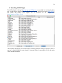
Fig 2 shows the interface for filterwheel control and option to add sequencing to by changing
Pockels cell value for each wavelength. Appendix B describes steps to follow for using filterwheel
sequencing with Pockels cell value. Pockels cell is used to regulate power from laser going to
sample. To use laser sequencing and filterwheel sequencing, it is desirable to adjust the Pockels
cell value so that the power of laser is within reasonable range, which is safe for the sample. User
can decide which filters to use for sequencing, add corresponding Pockels Cell value, check the
Sequence box and start the sequencing. WiscScan will collect the images in X-Y-Z location for
each of the filter and associated Pockels cell value. This feature has been tested and used by
biologist to look at SHG (Second Harmonic Generation) and GFP (Green Fluorescent Protein)
Images in Zebrafish. SHG and GFP has two vastly different signal intensities, SHG being very
faint and GFP being quite bright. This experiment requires changing the emission filter combined
with Pockels cell control to regulate power.
Fig 2. Filterwheel control from WiscScan with options to sequence using different Pockels cell
value
Filterwheel along with Pockels cell control is now part of main scanning code of WiscScan. The
information is now also being stored in metadata. One shortcoming it has which I am working on
now is- ability to stitch image, which are collected using this sequencing mode. There is a metadata
mismatch in the OME-TIFF files collected in this manner and as this method makes the image to
add one more dimension- it is difficult for image stitcher to parse images for proper location.
2.3 Neutral Density filter control:
Neutral density (ND) filter is adds another layer of control beside Pockels Cell to regulate power
from the laser. Neutral density filter reduces or modifies the intensity of all wavelength or colors
giving no changes in hue of color calibration.
ND filter Wheel comes with usually 6 or 12 position where we can insert filter to regulate power.
This is used in conjunction with Pockels cell because it gives wider range of power control and
user flexibility. For example, in SLIM system the accepted power level for lifetime imaging is 1%
or original power whereas 33% power is needed for regular imaging. This level of wider power
6
variation can be achieved by neutral density filter. We are using a Thorlabs FW102 filterwheel
that that has 6 position. I am currently using 2 position out of 6. One is using a ND filter allowing
33% power transmission (for regular imaging) and another position is using 1% power
transmission (for lifetime imaging). Whenever we switch acquisition mode to lifetime filterwheel
also moves to predefined position to allow allocated power. The FW102 filterwheel has its own
instruction set and can be controlled externally with RS232 port. Appendix C describes the
command set of filterwheel for serial control and C code to control from WiscScan.
2.4 White balance for white light image acquisition:
For many use cases, user would require high resolution brightfield image. This requires an
brightfield high resolution camera with high quantum efficiency. We use QImaging QIClick
camera in two of our systems. As the image sample is illuminated by external light (instead of
excitation by laser) the image is susceptible to color imbalance which makes co-registration of the
image challenging and often inaccurate. So dynamic white balance during live acquisition gets rid
of imbalance introduced by environment or settings in camera itself. I wrote a dynamic white
balance algorithm that enables user to automatically balance brightfield images during acquisition.
It also lets the user to manually adjust the value multipliers in R,G,B channel to use predefined
settings if the user has any preferences.
Fig 3: White Balance control Panel in WiscScan
2.4.1. White balance procedure:
There are many white balancing algorithm (22–27) yielding convincing results. Most of them are
based on dedicated hardware or Graphics Processing Unit. My priority was finding the one that is
faster so that the speed of acquisition is not compromised. The image frame from QCam is
1392x1040 pixels, the white balance algorithm needs to be fast enough to finish white balancing
the image in ~500 milliseconds. I investigated several white balancing algorithm and found that
algorithm based on Automatic white balance based Histogram Matching (25) is the most suitable
for our case. This implementation describes a method to match the histogram of the R,G, B color
channel by increasing the overlap area of the three channels. I used the idea of matching the
7
histogram of all three channel but in a less computational method. First, the histogram of all three
channel were calculated. The maxima of the histograms were calculated for all three channels. The
channel which had its peak in between the others, was selected as base channel. A multiplier was
calculated to match the other histogram to the base channel. These multipliers were multiplied to
their respective channels to form the color image again with the modified value. For the following
histogram of three R,G,B channel R has peak in between B and G. So the constants were calculated
as following
Gpeak
KG= Rpeak
Bpeak
KB= Rpeak
KR=1
Now all of the pixel value are recalculated with multipliers of KG, KR, KB.
Automatic white balance calculates the multiplier for all three channel and gives user live white
balanced image. Additionally, user can use the slider for each channel (fig 3) in WiscScan to
change the multiplier to have a different white balanced image.
Appendix D describes the coding of white balancing algorithm and integration with WiscScan
3. Fluorescence lifetime imaging (FLIM) setup
Fluorescence lifetime imaging (FLIM) depends on the fluorescence decay differences between
tissues to generate image contrast. FLIM has emerged as a powerful technique for observation of
proteins in living cells. FLIM can easily be applied to live cell and tissues as this method is
minimally invasive compared to other optical techniques. FLIM gives advantage in a way that it
can remotely monitor the local environment of a molecular probe independent of the fluorescence
intensity or local probe concentration. With the technological advances of optical microscopy
technique aided by development of powerful software has facilitated enormous image processing.
FLIM provides a sophisticated way of looking into cancer cell by looking into their local
environment and provides a way to look into metabolic activity of Nicotinamide adenine
dinucleotide (NADH).
The image obtained with FLIM is dependent largely on the concentration and intensity
independent but is sensitive to the environmental surroundings of the fluorophore for example pH
(28,29) , refractive index (30,31) or viscosity(32). In case of absence of contrast can be gained
using inherent auto fluorescence of many samples for many diagnostic purpose like for cancer
detection and treatment. (33,34). In cell biology FLIM is commonly used for measuring protein-
8
protein interaction visa Foster Resonance Energy Transfer (35). For a fluorophore with single
exponential decay, the intensity at time 𝑡 can be mathematically describes as
𝑡
….. (i)
𝐼(𝑡) = 𝐼(0) exp (− 𝜏) + 𝑐
Where 𝐼(𝑡) is the intensity after the excitation light has ceases and 𝐼(0) is the intensity at time 0.
Tau(𝜏) is the florescence lifetime defining the rate of decay. The constant c is the background light.
If there are two fluorophores, the intensity at time 𝑡 is
𝑡
𝑡
1
2
𝐼(𝑡) = 𝑎1 exp (− 𝜏 ) + 𝑎2 exp (− 𝜏 ) + 𝑐
…. (ii)
𝑎1 is the fractional contribution from fluorophore 1 and 𝑎2 is the fractional contribution from
fluorophore 2. 𝜏1 and 𝜏2 are the lifetime of the two components.
Fluorescence lifetime can be measured in time domain or frequency domain. Time correlated
single-photon counting (TCSPC) method is used to measure lifetime of a fluorophore. The
principle of TCSPC is the detection of single photon and measurement of their arrival time in
reference to its originating signal, the light source. It is a statistical method to accumulate sufficient
number of photon events for a required statistical precision. TCSPC in FLIM requires (18)i.
A high repetition rate laser to excite sample
ii.
A timing reference “sync” signal from the laser(Coherent laser)
iii.
A Scanning device that scans a spot or over a sample(WiscScan and microscope)
iv.
Output clock signal from scanning device- pixel clock, line clock, frame clock for
synchronization of the data acquisition(delivered by WiscScan)
v.
A port from microscope the delivers fluorescence photons to a detector(PMT)
vi.
A fast photon counting detector
vii.
A TCSPC module that builds up photon distribution over the arrival time of the photon
in the laser pulse period.
We have one lifetime board SPC-830 (36) board in our Optical Workstation System. SPC-830 has
a 4 times memory compared to previous SPC-730 board and has extremely fast bus interface. Even
in Scan Sync In mode SPC-830 provides large enough space to simultaneously record images in
multiple wavelengths or even multi spectral images. SPC-830 has been increasingly replaced by
SPC-150 board though it has a smaller memory. Becker & Hickl provides their own proprietary
software SPCM, which works as a standalone software for lifetime image acquisition. It can
control the acquisition parameters of the board. SPCM is compatible with all lifetime board from
Becker & Hickl Gmbh. and compatible acquisition mode. Becker & Hickl also provides complete
library(Appendix E) to control the image acquisition and parameter manipulation from external
program. Appendix E describes the library and flowchart of lifetime image acquisition sequence.
9
As mentioned earlier, our goal is to make a complete package for image acquisition for
multiphoton microscope we have already developed code for lifetime image acquisition in Scan
Sync in mode for the SPC-830 mode. This mode allows the image to be build up in the board’s
memory. After acquisition is finished, data is transferred to computer. Despite having some
advantages, this mode has some limitation 1) It depends on the memory on board, which does not
allow us to capture image larger than 256x 256, 2) During imaging users can’t see how the images
look like, have to wait till the end of the acquisition which typically is larger than 60 seconds. To
decide if that image is an acceptable or an unacceptable one, users will need to wait for the whole
acquisition to finish.
As data transfer rate increased overtime and Becker & Hickl introduced FIFO mode in its scanning
board which captures each frame and sends them to computer. FIFO mode has the advantage that
the user can observe the lifetime image as it gradually builds up and this data can be further utilized
for gathering information about the sample on-the-fly. If the user does not feel the photon count
does not look good or the focus is not good, the imaging can be cancelled before the pre-allocated
imaging time finish and move to the next location.
Having lifetime image updated after capturing every frame gives us the flexibility to analyze the
image on-the-fly (see section 5 for future development). The aim is to analyze the lifetime image
on-the-fly so that the fit gradually gets better with histogram of the decay curve populating
gradually. This way user can estimate how the lifetime values will approximate when analyzing.
Open source like SLIM Curve (see section 4) library helps us to achieve this goal. We can call
SLIM curve library to analyze every frame data after capturing and approximate lifetime values.
The fits get better as more and more photons are accumulated and timing constants approximation
gets better.
3.1 Lifetime board installation (SPC-150)
We installed a new lifetime system fully working now in our Spectral and lifetime Imaging. We
already have a fully functional lifetime board (SPC-830) in out optical workstation. For new
system, we opted for new SPC-150 board, which is more advanced in many aspects. As we use
our own scanning system controlled with WiscScan, the board should have all of its external
triggers and clock signals from WiscScan. Fig 4 describes the connection diagram for using with
external pixel clock.
WiscScan’s DSP produces the necessary clock signals for the imaging. There are three external
clock signals required as input to the board for successfully building up the image.
i)
Pixel Clock- Indicates that end of each pixel location
ii)
Line clock- Line clock indicates the end of line, after getting a line clock, it goes to a
new line
10
iii)
Frame clock- initiated after a frame is completed.
After line clock and frame clock there is a dead time associated with the fly back time from the
end of line/frame to the beginning of next line/frame.
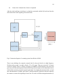
Fig 4: Connection diagram of a scanning system from Becker & Hickl
These is one challenge for using the external clock for the pixel clock is its high frequency.
WiscScan takes around 1 second to finish a 512 x 512 image. That gives one pixel 3.81 micro
second to complete. That is a effective frequency of 200KHz. At that frequency, the pixel clock
gets noisy and often misinterpreted. Becker & Hickl provides the option to use internal pixel clock,
which yields convincing results for optical workstation. To calculate the actual pixel time, we took
into consideration two variables, pixel time (T) and dead time(D). Dead time is the time taken for
the scanner to return to the beginning of a next line. We took two different integration number (I).
11
Integration time refers to how long the scanner stays at one pixel location. For example, if pixel
time is 2 microseconds and integration is 2, the scanner scans each pixel for 4 us. For two different
integration value(I), we measured the scanning time and formed two equations for finding the
exact value of T and D.
I * T*number of pixels + number of lines *D = (WiscScan time per frame)
Solving the two equations, we found the value of T to be 1.296, which translates to a pixel time of
2.6. We tuned the pixel with small increment and decrement to find the optimum value of 2.4. The
difference from the calculated value and actual value is because of the fly-back time after frame
completion. With this approach, we were able to find the exact value of pixel time that can be used
at any resolution. In future (see future expansion section), we plan to upgrade the system to FPGA
based system. Upon upgrading, we will use external clock from pixel, which is more accurate and
will not require tuning the value for every new system.
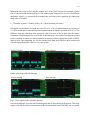
Before Filtering
After filtering
Frame clock before and after filtering
Before filtering
After filtering
Fig 5: Clock signals before and after filtering
Line clock and frame clock are both external signals and are generated from WiscScan. This clock
signals work fine for Optical workstation but the clock generated from SLIM DSP was very much
12
noisy to the extent that, even SPCM did not identify those clock signal as clock signals. To remove
noise, we setup new ribbon cable that carries the signal from DSP to Lifetime board. We setup a
low pass signal cutoff signal roughly at few kilohertz to attenuate the noise. Fig 5 shows the signal
before and after the filter circuit.
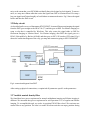
3.2 Relay circuit
As described earlier we use a Hamamatsu H7422L PMT. In normal fluorescent imaging the signal
from the PMT goes straight to the HFAC-26 (37) and this goes to DSP. For lifetime imaging we
setup a relay that is controlled by WiscScan. This relay routes the signal either to DSP for
fluorescent imaging or Lifetime board. For lifetime imaging, after PMT the signal goes to a
HFAC-26(Amplifier by Becker & Hickl) and then goes to SPC-150 board as CFD signal. Fig 6
shows the connection diagram of the relay, pre-amp and connection going to SPC150 and DSP.
Fig 6: connection diagram from PMT
After setting up physical connections, we optimized all parameters specific to the parameters.
3.3 Variable neutral density filter
We found that, laser power requirement for normal multiphoton imaging and lifetime imaging is
different. We measured that, power requirement for safe operation is 1% of regular non-lifetime
imaging. To accomplish this task, we used a six position FW102 filter wheel. We can insert one
custom filter to any position. The idea is to make WiscScan switch to an empty position during
13
regular imaging and move the wheel to the position where the filter is set during lifetime imaging.
The FW102 comes with its own instruction set which can be controlled via RS-232 port. Appendix
C describes the code and procedure for neutral density filter control.
Finally, after all the parameters were set, we measured Instrument response function at 2 most
used wavelengths (890nm and 740 nm). Fig 7 shows the instrument response functions at 890nm
and 740 nm wavelength in SLIM.
a.
b.
Fig 7: instrument response function at a)890 nm and b)740 nm
14
We compared lifetime of some standard samples and compared them with published values(38).
We found that the lifetime value of Coumarin 6 in ethanol to be 2.5 ns for a single exponential fit.
We measured the lifetime of YG beads (20 micrometers) and found the lifetime in SLIM and OWS
to be in agreement and also matches with the published value(2ns)(39)
3.4. Next steps:
Immediate next step is making WiscScan to work with FIFO acquisition mode. The architecture
of lifetime image acquisition as described in Appendix E, shows the frame after is finished an
WiscScan has the pointer to the location of the image in DSP’s memory. In FIFO architecture, the
frame is sent to PC after every capture. The existing architecture need is being modified to be
compatible with SPC150 board.
4. SLIM Curve:
As evident from discussion from the previous sections, there has been significant advances in
biological application and instrumentation there has been a lack of analysis tool for FLIM image.
Hardware manufacturer Becker and hickl provides their own software SPCImage for analyzing its
proprietary .SDT files. PicoQuant also provides proprietary software SymPhoTime 64 for
analyzing lifetime images in *.ICS format. But these are commercial packages and are closed
source tools that are not transparent in their analysis which only support only their own proprietary
format. One of the early effort for FLIM analysis tool is FLIMFit (20) . In effort to develop a
modular and flexible FLIM algorithm library that can be easily utilized and modified by developer
as well as easily usable by bench biologist, a library has been developed which is know as Spectral
Lifetime Imaging (SLIM) Curve. It is built on the previous effort in lifetime analysis (20,40) and
spectral lifetime analysis (41). SLIM Curve is an international collaboration between software
developers and microscopists at the Cancer Research UK and Medical Research Council Oxford
Institute for Radiation Oncology and Randall Division, King’s College London in the UK; and the
Laboratory for Optical and Computational Instrumentation (LOCI). SLIM curve library can be
used as standalone (from command prompt) or from a third party application like TRI2 (42) or
from ImageJ as a plugin(43) that can integrate FLIM with other image processing application. One
powerful advantage ImageJ offers in FLIM analysis is segmentation. Looking at the lifetime
distribution of a specific manually defined ROI can often be impossible or cumbersome at best,
with commercially available FLIM analysis software packages. ImageJ not only has conventional
manual and automatic segmentation, but in addition supports machine-learning-based
classification techniques (44) which can be exploited to use a training set to automatically segment
images in batch processing. One of the powerful features of ImageJ is macro language scripting
which enables the user to manually record (http://rsbweb.nih.gov/ij/docs/guide/146-14.html) a set
of operation using macro and repeat the set of operations without going through them manually
15
again. I worked on several major and minor features to improve the usability of SLIM plugin as a
standalone FLIM analysis tool so that it not only can be used a better alternative to other
proprietary FLIM analysis tool but also augments others usable feature of ImageJ. Beside several
small improvement, I worked primarily on
i)
Adding macro language support for all functions of SLIM Plugin
ii)
Make SLIM analysis work in conjunction with trainable WEKA segmentation
iii)
Test and compare results obtained with SLIM plugin with standard FLIM analysis tool
SPCImage
Apart from these changes, I also added some minor improvements. Some of them are- ability to
set default excitation and load default excitation when needed, exporting mean values to CSV files
for more flexible operation. Appendix G describes ways to install SLIM plugin.
4.1. Macro language support
SLIM plugin is a ImageJ plugin written in Java hosted in Github (https://github.com/slimcurve/slim-plugin). One of the most useful feature of ImageJ is macro scripting. A macro is a
simple program that automates a sequence of operations. A macro is created by recording a series
of command using the command recorder (Plugins>macro>Record). Later, the macro can be used
to execute the same series of operation. There is Recorder class for ImageJ, which is used for
recording commands as strings. Appendix F shows a sample operation for recording a macro from
the code.
4.2. Using segmentation
One of the great challenges in working with FLIM analysis is the processing time associated with
individually analyzing every image or a specific ROI in each image. For some samples, the
background comprises the majority of the image and affects the distribution of the overall lifetime.
Background should be excluded from the analysis to have greater accuracy. For example, to
examine a specific type of region in each image such as the cytoplasm or nucleus, manually
creating ROI for each one is often cumbersome, often inaccurate and very inefficient. With
advancement in supervised machine-learning-based techniques, it has become possible to
automatically segment specific regions based on training sets. For batch processing, it provides
the flexibility to exclude background or just look at specific types of regions such as the cytoplasm.
One of the widely used machine learning tools for supervised machine learning is Weka (45), a
tool which incorporates several machine learning techniques into a software library that can be
used externally used with Java.
Trainable Weka Segmentation (44) (http://fiji.sc/Trainable_Weka_Segmentation) is a Fiji plugin
that works with a set of features to produce pixel-based segmentation by using WEKA. It contains
the visualization tools together with a graphical user interface for ease of access to the user.
16
Appendix H describes step by step procedure to use Trainable WEKA segmentation for
segmenting FLIM image.
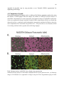
4.3 Comparison of result:
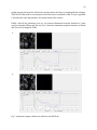
We demonstrated that SLIM plugin can be a viable tool for lifetime quantitative analysis by using
the features of SLIM plugin with real sample. We looked at NAD(P)H lifetime analysis of
subcellular compartments in a mouse pancreatic islet. Intensity images of NAD(P)H in pancreatic
islets were segmented in ImageJ using the Trainable WEKA segmentation. ROIs were created that
denote the nuclear, cytoplasmic and mitochondrial compartments and then the lifetime values for
each compartment were calculated using SLIM Curve. This powerful use case illustrates SLIM
Curve being combined with a popular and useful ImageJ plugin.
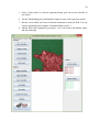
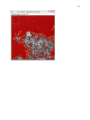
Fig 8. Lifetime analysis with SLIM Curve plugin using segmentation
NAD(P)H lifetime analysis of subcellular compartments in a mouse pancreatic islet. (A) Intensity
images of NAD(P)H were segmented in ImageJ using the Weka Segmentation plug-in. ROIs
17
denoting the nuclear, cytoplasmic and mitochondrial compartments are overlaid in pink. (B)
Lifetime values (A2) for each compartment were calculated using SLIM Curve.
4.3.1 Imaging. Islets were imaged in glass bottom dishes (WPI, Sarasota, FL) on a Nikon TE-300
inverted microscope equipped with a Plan Apo 60X/1.4NA Oil immersion objective (Nikon
Instruments, Melville, NY). Islets were submerged in a standard external solution containing, in
mM: 135 NaCl, 4.8 KCl, 5 CaCl2, 1.2 MgCl2, 20 HEPES, 10mM glucose; pH 7.35. Temperature
MD). NAD(P)H was excited with MaiTai Ti:Sapphire laser (SpectraPhysics, Palo Alto, CA) at
740nm with a 450/70 bandpass emission filter (Chroma Technology, Bellow Falls, VT) before
being collected by a Hamamatsu H7422P-40 GaAsP photomultiplier tube (Hamamatsu Photonics,
Bridgewater, NJ). FLIM images were collected at 256x256 resolution with 120 second collection
using SPC-830 Photon Counting Electronics (Becker & Hickl GmbH, Berlin, Germany). Urea
crystals were used to determine the Instrumentation Response Function (IRF) with a 370/10
bandpass emission filter (Chroma). Fig. 8 shows the result after islet compartment segmentation
and FLIM analysis.
5. Future development
The work described in the above sections are part of a continuous development and all of them
will be further developed as part of my effort to make microscopy fully automated and make
lifetime imaging a viable tool for understanding metabolism and disease detection. For fully
automated microscopy with multi parameter imaging, WiscScan should allow user to sequence
over any settings of Pockels cell, laser wavelength, filterwheel, gain of detector and be able to
stitch them with ImageJ/Fiji. As described, all these parameters are now part of WiscScan control
and need to be further extended to include changeability during sequencing. Without Stitching
support, it will further complicated for the user to distinguish images because images will be five
dimensional if user also include time series. These parameter settings will also be included in the
metadata.
Lifetime imaging is being used more and more as a viable tool for understanding metabolism in
human body. Understanding metabolism will be key to understanding many diseases progression,
metastasis and healing. But in terms of instrumentation and software, it is in nascent state. Most
important of that is speed. For getting a reliable data in time domain it takes more than 1 minutes
to look at a 256x256 image. This makes the work for a scientist to look at a very large sample very
tedious. An obvious next step is investigating ways to improve image acquisition faster. A standard
256 time bin is used for lifetime image acquisition. I will investigate ways to produce reliable
lifetime data with 64 or 128 time bins. Another immediate next step would be make WiscScan to
work with FIFO mode of imaging and run live analysis on each frames. As described earlier, open
source library SLIM curve gives us the flexibility to analyze lifetime image without the restriction
18
of the proprietary software. FIFO images are build up over time and the photon count accumulate
over time. Any fitting library should work on analyzing those frames and get an estimate of the
mean value of lifetime parameters. As time goes on, fit will be better and lifetime parameters’
estimate will get better. In this way the user has a better estimate on how the mean values would
look like prior to the time-consuming process of analyzing the image with SLIM Plugin or
SPCImage. I will also compare frequency domain acquisition and analysis to compare with time
domain acquisition. Frequency domain method by phase modulation method (19) is very fast
compared to time domain method(46). There has been development in time domain method which
claim 29fps speed for FLIM(47). I will investigate these methods to augment them in our imaging
system and analysis algorithm. Lack of support for stitching in FLIM image is another major
drawback for large scale imaging. One of the reason is unavailability of open file format FLIM.
The companies which makes the hardware, have their own proprietary format. I will work on using
the existing data file formats to make them compatible with stitching or work on different open
file format which can be supported by host of hardware and software.
6. Conclusion
In summary, I have worked on making image acquisition with microscopy more automated. I have
automated several hardware like laser, filterwheel, brightfield image to be controlled with
WiscScan which is integrated software for image acquisition. I have developed on multi parameter
sequencing which controls laser power and filter during 4D imaging. I have worked on installing
and optimizing a new lifetime board for FLIM acquisition. To analyze FLIM data I have been part
of a team for developing open source plugin for ImageJ that uses SLIM Curve, an open source
curve fitting library. As part of my ongoing research effort, I will continue making image
acquisition completely automated with 5 dimensional sequencing so that user can vary all the
external hardware setting associated with imaging. I will continue working on investigating faster
hardware with more precision for FLIM acquisition. With time domain image acquisition, I will
investigate ways to make it faster with existing hardware. To facilitate analysis, I will work on
making lifetime fitting on-the-fly with open source library so that user does not have to wait till
the end of an acquisition cycle to look at the lifetime distribution of a FLIM image. Frequency
domain analysis also prove to be an excellent alternative with phasor analysis, which proves to be
very fast compared to conventional curve fitting method. These improvements will enable
investigators to look at large samples with better lifetime distribution.
19
Appendix
A. Laser control with instruction set and controlling class
We have two kinds of Ti:Sa laser, Spectre-Physics Mai Tai and Coherent Chameleon, which can
be controlled by external serial command set. The serial command can be sent either by hyperterminal or by creating a serial interface in visual studio with library provided by National
instrument. The list of useful serial command for the Mai Tai laser is as following
Commands for Mai Tai Laser
Command
Operation
Turns on the pump laser
ON
? Reads and returns the output power, from 0
READ:POWer?
to 2.00 W, of the Mai Tai
Reads and returns the operating wavelength
READ:WAVelength?
SHUTter 1 opens the shutter. SHUTter 0
SHUTter n (1, 0)
closes the shutter.
Reads and returns the shutter status
SHUTter?
WAVelength nnn (in nm)
WAVelength:MAX? WAVelength:MIN?
Sets the wavelength of the laser
These queries return the maximum and
minimum values for the WAVelength
command.
Commands for Chameleon Laser
Commands
LASER =1
LASER=0
SHUTTER=n
WAVELENGTH=nnn
VW=nnn
?VW
?S
Operation
Switches the laser from STANDBY to ON
Puts the laser in Standby
n=0, closes the shutter
n=1, opens the shutter
Sets the wavelength of the laser to the specified
value of nnn in nanometers
Prints the current wavelength of the laser
Prints the status of the shutter
20
National instrument provides library with its rs232.h header file to include necessary functions to
talk to serial port.
To open a serial port:
int OpenComConfig (int portNumber, char deviceName[], long baudRate, int
parity,
int
dataBits,
int
stopBits,
int
inputQueueSize,
int
outputQueueSize);
To read from a serial port
int ComRdByte (int portNumber);
Reads a byte from the input queue of the port you specify.
Writing to a serial port
int ComWrt (int portNumber, char buffer[], size_t count);
Writes count bytes to the output queue of the specified port.
A sample function to read a string to a serial port is,
void ReadFromPort(int port, char *buf)
{
int i=0;
while(true){
//keeps reading till we break at the end of string
int temp;
temp = ComRdByte(port);
char ch;
ch = temp & 0x00FF;
//get char
if (ch==' ')
break;
buf[i++]=ch;
}
buf[--i]='\0';
}
Sample Code to open a shutter in Laser(Chameleon)
int ShutterOpenChameleon(int port){
char wavestr[20]="S=1";
WriteToPortChameleon(port,strcat(wavestr,"\r"));
return 0;
}
//end of string
//append to string
21
int WriteToPortChameleon(int port, char *str){
return ComWrt(port, str,strlen(str));
//return 0;
}
There is a generic MaitaiCtrlPage class that has all the generic function for laser control. Apart from the
functions that creates the GUI the following functions define some general working function of the laser.
Each of the function has its own description to call Chameleon laser or MaiTai laser. All the Mai Tai laser
related functions are in MAITAIIO.c and Chameleon laser related functions are described in ULTRAIO.cpp
file. The public functions of the generic laser class are described below with their respective description in
comment.
//function for generic laser control
float LaserPower();//used for reading laser power
float ReadLaserWavelength();//returns Laser wavelength
void SetWavelength(float nm);//sets the wavelength of the laser
float wavelengthmin();//gets minimum wavelength of the laser
float wavelengthmax();//gets maximum wavelength of the laser
void LaserShutter(int on);//sets laser shutter on/off
int ReadShutter(void);//reads shutter status
CEdit maiTaiWaveEditCurrent;
///generic laser code ends
void setLLaserType();//sets which type of laser is being used maitai/chameleon
void setUltraport(int portnumber);
CStatic maiTaiPowerReading;
CStatic maiTaiReadyDisplay;
CProgressCtrl maiTaiPowerGauge;
MaiTaiCtrlPage();
MaiTaiCtrlPage(MaiTaiCtrlDialog*,CWnd*, ControlPanel *);
~MaiTaiCtrlPage();
DECLARE_DYNCREATE(MaiTaiCtrlPage)
bool maiTaiReady;
//GETTERS
const bool GetMaiTaiCtrlPageCreated();
bool GetMaiTaiOnOff();
int GetDesiredWaveLength();
//SETTERS
void SetMaiTaiOnClose(bool);
22
B. Using Filter sequencing
SLIM system comes with its own filterwheel which can be controlled with WiscScan. SLIM does
not use an external manual filterwheel control. Now it has the ability to use any filterwheel to use
for sequencing. The steps are,
i.
Write the filters to be used for sequencing without any space in the space beside
“Sequence”. For example, if anyone wants to use filter number 3,4 and 8 for
sequencing, the user should write “348” in the box
ii.
Check “Sequence” checkbox
iii.
Set the pockel cell to desired value(which is to be used for first filter) and hit “Add
Pockels cell”. If there are 3 filters, 3 pockels cell value should be added.
iv.
Now starting sequencing with normal sequencing will start sequencing with desired
filter and pockel cell settings.
C. Neutral Density Filter-wheel control
We use a FW 102 Filterwheel for using the Neutral Density filters. This filterwheel has 6 empty
slots and can be controlled with button in the wheel or externally from the serial port. The settings
for connecting through serial port are,
- Baud Rate = 9.6K Bits Per Second
- Data Bits = 8
- Parity = None
- Stop Bits = 1
- Flow Control = None
The useful serial commands for controlling with RS232 port.
Command
Operation
pos=n
n=1-6, sets the filterwheel to n-th position
pos?
Returns the position of the current filterhwheel
trig=0
Sets the external trigger to the input mode
Trig=1
Sets the external trigger to the output mode
Here is sample code snippet for setting the filterwheel from Visual studio C.
Input parameters
Port- The port to which FW102 is connected,
Filter- Position of the filter where to move.
int setFilter(int port,int filter){
char wavestr[20]="pos=";
char portStr[10]="";
//char buffer=
strcat(wavestr,itoa(filter,portStr,10));
23
strcat(wavestr,"\r");
char buf[20]="";
int temp=WriteToPort(port,wavestr);
ReadFromPort(port,buf);
return temp;
}
D. White balance code
Assuming the data is arranged in RGB sequence for each pixel and each pixel value is saved as
unsigned character, the white balance code is as following,
The code assumes the input image is in 8-bit Bitmap format.
void whiteBalance(){
//
ReadBMP();//unsigned char *ReadBMP( char *f, int *width, int *height );
unsigned char *data;
int w,h,i,size,a1,a2,a3;
char *f="input.bmp";
data=readBMP(f,&w,&h);
size=w*h*3;
int a=-100;
//////the follwoing parameters are for histogram
int MaxArrayR[2];
int MaxArrayG[2];
int MaxArrayB[2];
int histoR[256]={};
int histoG[256]={};
int histoB[256]={};
///histogram parameters end
///generates histogram
for(i = 0; i < size; i += 3)
{
histoR[data[i]]++;
histoG[data[i+1]]++;
histoB[data[i+2]]++;
}
///calcualtes maximum of histogram
max(histoR,MaxArrayR);
max(histoG,MaxArrayG);
max(histoB,MaxArrayB);
24
int hmax1=MaxArrayR[1];
int hmax2=MaxArrayG[1];
int hmax3=MaxArrayB[1];
printf("\nmuahha =%d %d\n",MaxArrayR[0],MaxArrayR[1]);
int
midval=
(hmax1>hmax2)?(hmax1<hmax3?1:(hmax2>hmax3?2:3)):(hmax2<hmax3?1:(hmax1>hmax3?1:3));
///following code block finds the factors to add based on which histogram has teh
median value
switch(midval){
case 1:
a1=0;
a2=hmax1/hmax2;
a3=hmax1/hmax3;
break;
case 2:
a2=0;
a1=hmax2/hmax1;
a3=hmax2/hmax3;
break;
case 3:
a3=0;
a1=hmax3/hmax1;
a2=hmax3/hmax2;
break;
printf("\nhistogram data\n maxs %d %d %d a1=%d a2=%d a3=%d, midval=%d\n",hmax1,hmax2,hmax3,
a1,a2,a3,midval );
///test image write code segment
for(i = 0; i < size; i += 3)
{
data[i]=clip(data[i],a1);
data[i+1]=clip(data[i+1],a2);
data[i+2]=clip(data[i+2],a3);
}
WriteBMP("output.bmp",w,h, data);
}
unsigned char clip(unsigned char imvalue, int multiplier){
int temp=imvalue*multiplier;
25
if(temp>255) temp=255;
if(temp<0) temp=0;
return (unsigned char)temp;
}
void max(int *hist, int *locArray){
int max=-100;
int i;
for(i=0;i<256;i++){
if(hist[i]>max){
max=hist[i];
locArray[1]=i;
}
}
locArray[0]=max;
}
E. Lifetime acquisition library and flowchart of lifetime imaging
Becker and Hickl provides SPCM Dynamic Link Library which contains all functions to control
the whole family of SPC modules which work in the PCI bus. To install the DLLs, the TCSPC
package should be downloaded from http://www.becker-hickl.com/ . The DLLs have all the
functionalities implemented though we use some of them for initializing, setting parameter, saving
image and stopping measurement. All the functions are listed in SPCM DLL manual (48). Some
important library functions are described below,
short CVICDECL SPC_init (char * ini_file);
Input parameters:
* ini_file: pointer to a string containing the name of the initialisation file in use (including file
name and extension)
Return value:
0 no errors, <0 error code
Description:
26
Before a measurement is started the measurement parameter values must be written into the
internal structures of the DLL functions (not directly visible from the user program) and sent to
the control registers of the SPC module(s). This is accomplished by the function SPC_init.
short CVICDECL SPC_set_parameters(short mod_no, SPCdata *data);
Input parameters:
mod_no 0 .. 7, SPC module number
*data pointer to result structure (type SPCdata)
Return value: 0 no errors, <0 error code (see spcm_def.h)
The procedure sends all parameters from the ‘SPCdata’ structure to the internal DLL structures
of the module ‘mod_no’ and to the control registers of the SPC module ‘mod_no’.
short CVICDECL SPC_start_measurement(short mod_no);
Input parameters:
mod_no 0 .. 7, SPC module number Return value: 0: no errors, <0: error code
The procedure is used to start the measurement on the SPC module ‘mod_no’. Before a
measurement is started by SPC_start_measurement
- the SPC parameters must be set (SPC_init or SPC_set_parameter(s) ),
- the SPC memory must be configured ( SPC_configure_memory in normal modes),
- the measured blocks in SPC memory must be filled (cleared) (SPC_fill_memory),
- the measurement page must be set (SPC_set_page)
short CVICDECL SPC_stop_measurement(short mod_no);
Input parameters:
mod_no 0 .. 7, SPC module number
Return value: 0: no errors, <0: error code
27
The procedure is used to terminate a running measurement on the SPC module ‘mod_no’.
Because of hardware differences the procedure action is different for different SPC module
types.
short CVICDECL SPC_fill_memory(short mod_no, long block, long page, unsigned short
fill_value);
The procedure is used to clear the measurement memory before a new measurement is started.
short CVICDECL SPC_read_data_block( short mod_no, long block, long page, short
reduction_factor, short from, short to,
unsigned short *data);
The procedure reads data from a block of the SPC memory (on module ‘mod_no’) defined by the
parameters ‘block’ and ‘page’ to the buffer ‘data’. The procedure is used to read measurement
results from the SPC memory.
short CVICDECL SPC_write_data_block(short mod_no, long block, long page, short from,
short to, unsigned short *data);
The procedure reads data from the buffer ‘data’ in the PC and writes it to a block of the memory
defined by the parameters ‘block’ and ‘page’ on the SPC module ‘mod_no’. The procedure is
used to write data from the from PC memory to the memory of the SPC module.
short CVICDECL SPC_read_fifo (short mod_no, unsigned long * count, unsigned short
*data);
The procedure reads data from the FIFO memory of SPC modules SPC6x0/13x/830/140/15x/160 and has no effect for other SPC module types. Because of hardware
differences the procedure action is different for different SPC module types.
There are also some functions to regulate the imaging process more with more precision and they
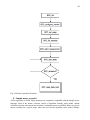
are used in WiscScan. WiscScan has a spate class for LifeTimeCtrlPage which has all the
imaging functions implemented. The flowchart for lifetime image acquisition is given below,
28
Fig: 9 Lifetime acquisition flowchart
F. Sample macro recorder
All the operations in SLIM Plugin operation are completely compatible with the ImageJ macro
language. Each of the button, selection, choice of algorithm, binning, noise model, default
excitation selection with custom start-end time is completely macro record-able. Below is a typical
macro recording for a typical usage where the user sets the algorithm, noise model, changes
29
transient time, loads default excitation, sets the chi2 target, fixes A value for fitting and then starts
fitting.
call("loci.slim.SLIMProcessor.startSLIMCurve",
"/4t1_740_60xW_zoom4_256_1mg_1_140218_copy.sdt");
run("SLIM Curve");

Change the algorithm:
call("loci.slim.SLIMProcessor.setAlgorithmType",
RLD");

"true",
"SLIMCurve
Set number of components of exponents:
call("loci.slim.SLIMProcessor.setFunctionType",
Exponential");

"Double
Change noise model:
call("loci.slim.SLIMProcessor.setNoiseModel","Poisson Data");

change which parameters for fitting:
call("loci.slim.SLIMProcessor.setFittedImagesType", "3");

Set transient start time:
call("loci.slim.SLIMProcessor.setTransientStart", "2.0");

Set the binning
call("loci.slim.SLIMProcessor.setBinnning", "3 x 3");

Load default excitation:
call("loci.slim.SLIMProcessor.loadDefaultExcitation", "true");

Load default excitation:
call("loci.slim.SLIMProcessor.loadDefaultExcitation", "true");

Set the chi2 target value:
call("loci.slim.SLIMProcessor.setChi2Target", "1.75");
 Fix the A value(All "fix" are recordable):
call("loci.slim.SLIMProcessor.fixA1", "true");

Start fitting
call("loci.slim.SLIMProcessor.startFitting", "");

Loading an existing excitation file
30
call("loci.slim.SLIMProcessor.setExcitation",
"/Users/msagar/Documents/qwe.irf");

Set to double exponential(no of component =2)
call("loci.slim.SLIMProcessor.setFunctionType", "Double Exponential");

Fix Z for double exponential fitting
call("loci.slim.SLIMProcessor.fixZ", "true");
For batch processing, the whole operation can be recorded. Macro record the name of the files
needed for exporting the values. A typical batch processing macro code looks like following
 Start fitting
call("loci.slim.SLIMProcessor.batchModeSet", "true");
call("loci.slim.SLIMProcessor.exportFileSet",
"pixel.tsv",
"summary.tsv");
call("loci.slim.SLIMProcessor.startBatchMacro", "");
"histograms.t
When "Export Histogram to Text" or/and "Export Pixels to Text" is selected for exporting the
output to a CSV or TSV file that is also recorded in macro. A typical code looks like this
call("loci.slim.SLIMProcessor.exportHistoFileName", "histoGram.csv", ",");
call("loci.slim.SLIMProcessor.exportPixelFileName", "pixel.csv", ",");
call("loci.slim.SLIMProcessor.setAnalysisList", "true", "2");
Complete macro example with exporting histograms and pixel information to CSV file
call("loci.slim.SLIMProcessor.startSLIMCurve",
"true",
"/Users/msagar/Downloads/", "/4t1_740_60xW_zoom4_256_1mg_1_140218_copy.sdt");
run("SLIM Curve");
call("loci.slim.SLIMProcessor.setFunctionType", "Double Exponential");
call("loci.slim.SLIMProcessor.loadDefaultExcitation", "true");
wait(1000);
call("loci.slim.SLIMProcessor.setWidthPrompt", "1.8359");
call("loci.slim.SLIMProcessor.setWidthPrompt", "4.8533");
call("loci.slim.SLIMProcessor.setDelayPrompt", "-0.3791");
call("loci.slim.SLIMProcessor.setBinnning", "3 x 3");
call("loci.slim.SLIMProcessor.fixZ", "true");
wait(1000);
call("loci.slim.SLIMProcessor.startFitting", "");
call("loci.slim.SLIMProcessor.exportHistoFileName", "histogram1.csv", ",");
call("loci.slim.SLIMProcessor.exportPixelFileName", "pixel1.csv", ",");
call("loci.slim.SLIMProcessor.setAnalysisList", "true", "2");
31
G. Installing SLIM Plugin
The SLIM plugin for ImageJ (http://imagej.net/SLIM_Curve) is available via an ImageJ update
site. To start using it, download the Fiji distribution of ImageJ for the life sciences (http://fiji.sc/),
and enable the SLIM Curve update site as described on the ImageJ wiki
(http://imagej.net/Update_Sites).
Once installed, the plugin is accessible from the Lifetime submenu of ImageJ’s Analyze menu. It
can also be launched quickly using ImageJ’s Command Finder by pressing the L key and typing
“slim” into the search box
32
.
H. Segmentation of FLIM using Trainable Weka segmentation
ImageJ is powerful open source Java based software for image processing and extensively used by
biologists for microscopic image processing. ImageJ provides wide array of additional
functionality through its plugins. Fiji is a distribution of ImageJ with more plugins bundles with
it. Trainable Weka segmentation is plugin that can be used for machine learning based
segmentation in any image supported by ImageJ/Fiji. The general approach for using Trainable
Weka Segmentation is finding regions, adding them to different classes, train the classifier and use
that trained data to segment same/other images. The same approach can be used for FLIM images
and Fiji’s ROI manager can be used to create mask and exclude any region not needed. The steps
are as following,
1. Open a lifetime image using the SLIM Curve plugin.
2. Train the classifier using Trainable Weka Segmentation.
3. Create instances to train your classifier with the number of classes required.
4. Train classifier by clicking the "Train classifier" button.
33
5. Select “Create result” to create the segmented image (you can save the classifier to
use it later).
6. Use the Thresholding tool to threshold the image to remove the region not needed.
7. Run the Create Mask and Create Selection commands to make the ROI. You can
execute commands easily using the Command Finder (press L ).
8. Add the ROI to ROI manager by pressing T. Use it on overlay with lifetime image
and start analyzing.
34
35
References
1.
Wang W, Wyckoff JB, Frohlich VC, Oleynikov Y, Hüttelmaier S, Zavadil J, et al. Single
cell behavior in metastatic primary mammary tumors correlated with gene expression
patterns revealed by molecular profiling. Cancer Res. 2002 Nov 1;62(21):6278–88.
2.
Wolf K, Mazo I, Leung H, Engelke K, Andrian UH von, Deryugina EI, et al. Compensation
mechanism in tumor cell migration: mesenchymal-amoeboid transition after blocking of
pericellular proteolysis. J Cell Biol. 2003 Jan 20;160(2):267–77.
3.
Campagnola PJ, Millard AC, Terasaki M, Hoppe PE, Malone CJ, Mohler WA. ThreeDimensional High-Resolution Second-Harmonic Generation Imaging of Endogenous
Structural Proteins in Biological Tissues. Biophys J. 2002 Jan;82(1):493–508.
4.
Campagnola PJ, Clark HA, Mohler WA, Lewis A, Loew LM. Second-harmonic imaging
microscopy of living cells. J Biomed Opt. 2001 Jul;6(3):277–86.
5.
Campagnola P. Second Harmonic Generation Imaging Microscopy: Applications to
Diseases Diagnostics. Anal Chem. 2011 May 1;83(9):3224–31.
6.
Zipfel WR, Williams RM, Christie R, Nikitin AY, Hyman BT, Webb WW. Live tissue
intrinsic emission microscopy using multiphoton-excited native fluorescence and second
harmonic generation. Proc Natl Acad Sci U S A. 2003 Jun 10;100(12):7075–80.
7.
Hoover EE, Squier JA. Advances in multiphoton microscopy technology. Nat Photonics.
2013 Feb;7(2):93–101.
8.
Linkert M, Rueden CT, Allan C, Burel J-M, Moore W, Patterson A, et al. Metadata matters:
access to image data in the real world. J Cell Biol. 2010 May 31;189(5):777–82.
9.
WiscScan: a software defined laser-scanning microscope. Scanning.
10. Zimmermann T, Rietdorf J, Pepperkok R. Spectral imaging and its applications in live cell
microscopy. FEBS Lett. 2003 Jul 3;546(1):87–92.
11. Pappajohn DJ, Penneys R, Chance B. NADH spectrofluorometry of rat skin. J Appl
Physiol. 1972 Nov;33(5):684–7.
36
12. Chance B, Williamson J, Jamieson D, Schoener B. Properties and kinetics of reduced
pyridine nucleotide fluorescence of the isolated and in vivo rat heart. Biochem Z.
1965;341:357–77.
13. Ramanujam N, Mitchell MF, Mahadevan A, Warren S, Thomsen S, Silva E, et al. In vivo
diagnosis of cervical intraepithelial neoplasia using 337-nm-excited laser-induced
fluorescence. Proc Natl Acad Sci U S A. 1994 Oct 11;91(21):10193–7.
14. Schomacker KT, Frisoli JK, Compton CC, Flotte TJ, Richter JM, Nishioka NS, et al.
Ultraviolet laser-induced fluorescence of colonic tissue: Basic biology and diagnostic
potential. Lasers Surg Med. 1992 Jan 1;12(1):63–78.
15. Gupta PK, Majumder SK, Uppal A. Breast cancer diagnosis using N2 laser excited
autofluorescence spectroscopy. Lasers Surg Med. 1997;21(5):417–22.
16. Majumder SK, Gupta PK, Jain B, Uppal A. UV excited autofluorescence spectroscopy of
human breast tissue for discriminating cancerous tissue from benign tumor and normal
tissue. Lasers Life Sci. 1999;8(4):249–64.
17. Bastiaens PIH, Squire A. Fluorescence lifetime imaging microscopy: spatial resolution of
biochemical processes in the cell. Trends Cell Biol. 1999 Feb 1;9(2):48–52.
18. Becker W, Bergmann A, Hink M a., König K, Benndorf K, Biskup C. Fluorescence lifetime
imaging by time-correlated single-photon counting. Microsc Res Tech. 2004 Jan
1;63(1):58–66.
19. Gratton E, Breusegem S, Sutin J, Ruan Q, Barry N. Fluorescence lifetime imaging for the
two-photon microscope: time-domain and frequency-domain methods. J Biomed Opt.
2003;8(3):381–90.
20. Warren SC, Margineanu A, Alibhai D, Kelly DJ, Talbot C, Alexandrov Y, et al. Rapid
global fitting of large fluorescence lifetime imaging microscopy datasets. PloS One.
2013;8(8):e70687.
21. Huo J, Chang Y, Wang J, Wei X. Robust automatic white balance algorithm using gray
color points in images. IEEE Trans Consum Electron. 2006 May;52(2):541–6.
37
22. Lin J. An Automatic White Balance Method Based on Edge Detection. In: 2006 IEEE
Tenth International Symposium on Consumer Electronics, 2006 ISCE ’06. 2006. p. 1–4.
23. Weng C-C, Chen H, Fuh C-S. A novel automatic white balance method for digital still
cameras. In: IEEE International Symposium on Circuits and Systems, 2005 ISCAS 2005.
2005. p. 3801–4 Vol. 4.
24. Huang C, Zhang Q, Wang H, Feng S. A Low Power and Low Complexity Automatic White
Balance Algorithm for AMOLED Driving Using Histogram Matching. J Disp Technol.
2015 Jan;11(1):53–9.
25. Wang P-M, Fuh C-S. Automatic White Balance with Color Temperature Estimation. In:
International Conference on Consumer Electronics, 2007 ICCE 2007 Digest of Technical
Papers. 2007. p. 1–2.
26. Huo J, Chang Y, Wang J, Wei X. Robust automatic white balance algorithm using gray
color points in images. IEEE Trans Consum Electron. 2006 May;52(2):541–6.
27. Hille C, Berg M, Bressel L, Munzke D, Primus P, Löhmannsröben H-G, et al. Time-domain
fluorescence lifetime imaging for intracellular pH sensing in living tissues. Anal Bioanal
Chem. 2008 Jul;391(5):1871–9.
28. Nakabayashi T, Wang H-P, Kinjo M, Ohta N. Application of fluorescence lifetime imaging
of enhanced green fluorescent protein to intracellular pH measurements. Photochem
Photobiol Sci Off J Eur Photochem Assoc Eur Soc Photobiol. 2008 Jun;7(6):668–70.
29. Tregidgo C, Levitt JA, Suhling K. Effect of refractive index on the fluorescence lifetime of
green fluorescent protein. J Biomed Opt. 2008 Jun;13(3):031218.
30. van Manen H-J, Verkuijlen P, Wittendorp P, Subramaniam V, van den Berg TK, Roos D, et
al. Refractive index sensing of green fluorescent proteins in living cells using fluorescence
lifetime imaging microscopy. Biophys J. 2008 Apr 15;94(8):L67–9.
31. Kuimova MK, Yahioglu G, Levitt JA, Suhling K. Molecular Rotor Measures Viscosity of
Live Cells via Fluorescence Lifetime Imaging. J Am Chem Soc. 2008 May
1;130(21):6672–3.
38
32. Galletly NP, McGinty J, Dunsby C, Teixeira F, Requejo-Isidro J, Munro I, et al.
Fluorescence lifetime imaging distinguishes basal cell carcinoma from surrounding
uninvolved skin. Br J Dermatol. 2008 Jul;159(1):152–61.
33. De Beule P a. A, Dunsby C, Galletly NP, Stamp GW, Chu AC, Anand U, et al. A
hyperspectral fluorescence lifetime probe for skin cancer diagnosis. Rev Sci Instrum. 2007
Dec;78(12):123101.
34. Jares-Erijman EA, Jovin TM. Imaging molecular interactions in living cells by FRET
microscopy. Curr Opin Chem Biol. 2006 Oct;10(5):409–16.
35. Becker, W. The bh TCSPC Handbook. 6th ed. Becker & Hickl Gmbh; 2014.
36. HFAC-26 amplifier [Internet]. Available from:
http://www.photonicsolutions.co.uk/product-detail.php?prod=6130
37. Kristoffersen AS, Erga SR, Hamre B, Frette Ø. Testing Fluorescence Lifetime Standards
using Two-Photon Excitation and Time-Domain Instrumentation: Rhodamine B, Coumarin
6 and Lucifer Yellow. J Fluoresc. 2014 May 28;24(4):1015–24.
38. Skala MC, Riching KM, Gendron-Fitzpatrick A, Eickhoff J, Eliceiri KW, White JG, et al.
In vivo multiphoton microscopy of NADH and FAD redox states, fluorescence lifetimes,
and cellular morphology in precancerous epithelia. Proc Natl Acad Sci U S A. 2007 Dec
4;104(49):19494–9.
39. Barber PR, Vojnovic B, Atkin G, Daley FM, Everett SA, Wilson GD, et al. Applications of
cost-effective spectral imaging microscopy in cancer research. J Phys Appl Phys. 2003 Jul
21;36(14):1729.
40. Rueden C, Eliceiri KW, White JG. VisBio: A Computational Tool for Visualization of
Multidimensional Biological Image Data. Traffic. 2004 Jun 1;5(6):411–7.
41. Barber PR, Ameer-Beg SM, Gilbey J, Carlin LM, Keppler M, Ng TC, et al. Multiphoton
time-domain fluorescence lifetime imaging microscopy: practical application to protein–
protein interactions using global analysis. J R Soc Interface. 2009 Feb 6;6(Suppl 1):S93–
105.
39
42. Schneider CA, Rasband WS, Eliceiri KW. NIH Image to ImageJ: 25 years of image
analysis. Nat Methods. 2012 Jul;9(7):671–5.
43. Arganda-Carreras I, Cardona A, Kaynig V, Schindelin J. Trainable Weka Segmentation
[Internet]. [cited 2015 Jun 27]. Available from: http://fiji.sc/Trainable_Weka_Segmentation
44. Hall M, Frank E, Holmes G, Pfahringer B, Reutemann P, Witten IH. The WEKA Data
Mining Software: An Update. SIGKDD Explor Newsl. 2009 Nov;11(1):10–8.
45. Buranachai C, Kamiyama D, Chiba A, Williams BD, Clegg RM. Rapid Frequency-Domain
FLIM Spinning Disk Confocal Microscope: Lifetime Resolution, Image Improvement and
Wavelet Analysis. J Fluoresc. 2008 Mar 7;18(5):929–42.
46. Elson DS, Munro I, Requejo-Isidro J, McGinty J, Dunsby C, Galletly N, et al. Real-time
time-domain fluorescence lifetime imaging including single-shot acquisition with a
segmented optical image intensifier. New J Phys. 2004 Nov 1;6(1):180.
47. SPCM Dynamic Link Libraries; User Manual for SPC Modules. Becker & Hickl Gmbh;
2014.