Download Considering Uncertainty in Project Selection Decision Using Crystal

.19
OF RISK
1 .6 CONFR O NTI NG UNCERTAI NTY_THE M A N A G E M E N T
ahle 1-1
Sinole-Point Estimates of the Cash Flows tor
D
c
B
A
I
2
Year
3
A
't
2000*
Outflow
Inflow
p=(B-C)
C
B
Net Flow
Inc.
erami c S ci ences,lnc
E
F
G
Discount
Net Present
lnflation
Value
Rate
Factor
t l(1 -+ k + p )'
D x (Disc. Factor)
$o $125,000 -$125,000
1.0000
-$125,000
2000
0
100,000
-$100,000
0.8696
-$86,957
0.02
6
2001
0
90,000
-$90,000
0.756r
-$68,053
0.02
7
z00z
50,000
8
2003
t20,000
9
2004
115,000
10
7005
105,000
11
7.006
97,000
12
2007
90,000
IJ
2008
82,000
r4
2009
65,000
l)
2009
35,000
$50,000
0.6575
$32,876
$105,000
0.5718
$60,034
$115,000
0.4972
$57,175
$90,000
0.4323
$38,909
$97,000
0.3759
$36,466
0.02
$75,000
0.3269
$24,518
0.02
0
$82,000
0.2843
$23,310
0
$65,000
0.2472
$16,067
$35,ooo
0.2472
$8,651
0
15,000
0
15,000
n
15,000
0.02
I6
1,1
II
Total
$759,000 $360,000
$399,000
$t7,997
18
* t : 0at t
19
beginning of 2000
z0
21
Formulae
22
Cell D4
: (84 - C4) copyto D5:D15
L.)
Cell E4
: u(1 + .13+ .OZ;ns
1A
Cell E5
z5
z6
z7
CellE6
: 1/(1+ .13+ .02)^1
copyto F,1-!
: 1/(1+ .13+ .02)^(A6- 1.999)
Cell F4
: D4*E4 copyto F5:F15
Cell817
: Sum(B4:B15) copyto C1 , D17,F17
give us a reasonably good
Therefore, we will assumethat the triangular distribution will
fit for the inflow variables.
remaining vari'
The hurdle rate of fetum is typically fixed by the firm, so the only
factor' We have as'
able is the rate of inflation that is included in finding the discount
plus or minus 1 percent
sumed a 2 percent rate of inflation with a normal distribution,
(i.e., 31 percent represents+3 standarddeviations)'
most likely estiIt is important to point out that approaches in which only the
to assuming that the input data are
mate of each variable is used .t"
"q,tlrrul.nt
it allows all possible
known with certainty. The major benefit of simulation is that
of possible values for
values for each variable to be considered. Just as the distribution
likely" value, the disa variable is a better reflection of reality ihan the single "most
of an uncertain
tribution of outcomes developed by simulation is a better forecast
20.
C H A P T E R 1 / l H E WO R L D O F P R O J E C T M A N A G E MEN T
Table 1-2 Pessimistic,
Most Likely,and Optimistic
Estimatesfor CashInflowsfor PsychoCeramicSciences,Inc.
Minimum
Most Likely
Maximum
Year
lnflow
lnflow
lnflow
2002
$35,000
$50,000
$60,000
2003
$120,000
$136,000
2004
$95,000
$100,000
$115,000
$125,000
2005
$88,000
$105,000
$116,000
2006
$80,000
$97,000
$108,000
2007
$75,000
$90,000
$100,000
2008
$67,000
$82,000
$91,000
2009
$51,000
$65,000
$73,000
2009
$30,000
$35,000
$38,000
Total
$621,000
$759,000
$847,000
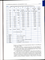
future reality than is a forecastof a single outcome. In general,preciseforecastswill
be "preciselywrong,"
Using CB to run a Monte Carlo simulation requiresus to definetwo tlpes of cells in
the Excel@spreadsheet.
The cells that contain variablesor parametersthat we make assumptionsabout are defined as assunrption
cells.For the PsychoCeramicSciencescase,
theseare the cells in Table 1.L, columnsB and G, the in{lowsand the rate of inflation,
respectively.As noted above,we assumethat the rate of inflation is normally distributed with a meanof 2 percent and a standarddeviation of .33 percent.Likewise,we assumethat yearlyinflowscan be modeledwith a triangular distribution.
The cells that contain the outcomes(or results)we are interestedin forecastingare
calledforecastcells.In PsychoCeramic's
casewe want to predict the NPV of the project.
Hence,cell F17 in Table 1-1 is definedasa forecastcell. Eachforecastcell rypicallycontains a formula that is dependenton one or more of the assumptioncells. Simulations may
have many assumptionand forecastcells,but they musthave at leastone of each.Before
proceeding,openCrystalBall@and makean Excel@spreadsheet
copyof Table 1-1.
process
cell,
consider
cell 87, the cash
To illustrate the
of defining an assumption
minimum
expectedcash
inflow estimatefot 2002. !7e can seefrom Table 1-2 that the
is $60,000.
and
the
maximum
inflow is $35,000,the most likely cashflow is $50,000,
triangular
distribution.
Also rememberthat we decidedto model all theseflowswith a
Given the information in Table l-7, the processof definingthe assumptioncellsand
enteringthe pessimisticand optimistic data is straightforwardand involvessix steps:x
1. Click on cell B7 to identifu it asthe relevant assumptioncell.
2. Selectthe menu option Cell at the top of the screen.
3. From the dropdown menu that appears,selectDefine Assumption. CB's Distribu.
tion Gallery is now displayedasshown in Figure1-6. (Note: it is important that the
* It is generally helpful for the reader to work the problem as we explain it. If Crystal Ball@has been installed
on your computer but is not running, select Tools, and then Add.ins from Excel@'smenu. Next, click on the CB
checkbox and select OK. If the CB Add-In has not been installed on your computer, consult your Excel@manual
and the CD-ROM that accomoaniesthis book to install it.
.21
1.6 CO NFRO NTI NG UNCERTAI NTY- T H E M A N A G E M E N T O F R I S K
!ognomal
l'
lirreihtdl
Unifcrs
L-
LT
ll,
lffil
9"r'r! I
Ctglm
Hygg#r;c
Setg
ta
Figure1-6 Crystal
Ball@2000Distribution Gallery.
Erwcr*id
II
ldM &
Eoryi
rq- |
Hrh I
cell being defined as an assumptioncell contain a numeric value. If the cell is empty
or contains a label, an error messagewill be displayedduring this step.)
4. CB allows you to choose from a wide variety of probability distributions. Doubleclick on the Triangular box to select it.
5. CB's Triangular Distribution dialog box is displayed as in Figure 1-7. In the
Assumption Name: textbox at the top of the dialog box enter a descriptive label,
for example, Cash Inflow 2002. Then enter the pessimistic, most likely, and
f-ryr-l
l*p'* I
JF
5
.tl
dt
.gt
ct.
L
IL
41250
Figure 1-? Crystal
Ball@2000 dialog
box for model
inputs assuming
the triangular
distribution.
47.ffi
53,ffi
60,m
{ fso'ooo
uinl$llEl!
r@
Liketie$*511,000
_g5J !ln9?ri t-Errt"l
Ha< !S1t,000
sdreryi cqryrtte,:.
i
22.
C H A P T E R 1 / T H E WO R L D O F P R O J E C T M A N A G E MEN T
optimistic costsof $35,000,$50,000,and $60,000in the Min, Likeliest, and Max
boxes,respectively.
6. Click on the OK button. (\Uhen you do this step,note that the inflow in cell B7 automatically changesfrom the most likely entry, or other numberyou might have entered, to the mean of the rriangular distribution which is (Min f Likeliest *
Max)/3.
Now repeatsteps1-6 for the remainingcashinflow assumptioncells (cells B8:B15).
Rememberthat the proper information to be enteredis found in Table 1.2.
When finishedwith the cashinflow cells,assumptioncellsfor the inflation valuesin
column G needto be defined.For thesecellsselectthe Normal distribution.We decided
earlier to usea 2 percent inflation rate, plus or minus 1 percent.Recall that the normal
distribution is bell-shapedand that the meanof the distribution is its centerpoint. Also
recall that the mean,plus or minus three standarddeviationsincludes99i percent of
the data.The normal distribution dialogbox, Figure1-8,callsfor the distribution'smean
and its standarddeviation. The meanwill be 0.02 (2 percent) for all cells.The standard
deviation will be .0033 (one-third of 1 percent). (Note that Figure1-8 displaysonly the
first two decimalplacesof the standarddeviation.The actualstandarddeviation of .0033
is usedby the program.)As you enter this data you will note that the distribution will
showa meanof 2 percentand a rangefrom 1 percentto 3 percent.
Notice that there are two cash inflows for the year 2000, but one of those occurs at
the beginning of the year and the other at the end of the year.The entry at the beginning
of the yearis not discountedso there is no needfor an entry in G4. (Someversionsof CB
insist on an entry, however, so go aheadand enter 2 percent with zero standarddeviation.) Move on to cell G5, in the Assumption Name: textbox for the cell G5 enterInfla.
tion Rate.Then enter .02 in the Mean textbox and .0033in the Std Dev textbox. While
the rateof inflation could be enteredin a similarfashionfor the followingyears,a moreefficient approachis to copy the assumptioncell G5 to G6:G14. Becausethe inflation rate
is now a variable,we mustchangethe formulaefor column E asnoted in Table 1-3.Since
Figure1-8 Crystal
Ball@2000 dialog
box for model
inputs assuming
the normal
distribution.
1.6 CON FRO NTI NG UNCERTAI NTY_T H E M A N A G E M E N T O F R I S K
.23
CB is an add-in to Excel@, simply using Excel@'scopy and paste commands will not
work. Rather, CB's own copy and paste commands must be used to copy the inforrnation conrained in both assumption and forecast cells. The following steps are required:
1. Place the cursor on cell G5.
2. Enter the command Cell, then click on Copy Data.
3. Highlight the range G6:G14.
4. Enter the command Cell, then Paste Data.
Note that the year 2009 has two cash inflows, both occurring at the end of the year.
Because we don't want to generate two different rates of inflation for 2009,
the value generated in cell G14 will be used for both 2009 entries. In cell G15 simply
enter =G14.*
Now we consider the forecast or outcome cell. In this example we wish to find the
net present value of the cash flows we have estimated. The processof defining a forecast
cell involves five steps.
1. Click on the cell F17 to identify it as containing an outcome that interests us.
2. Select the menu option Cell at the top of the screen.
3. From the dropdown menu that appears,select Define Forecast . . .
4. CB's Define Forecast dialog box is now displayed. In the Forecast Name: textbox,
enter a descriptive name such as Net PresentValue of Project.Then enter a descriptive label such as Dollms in the Units: textbox.
.5. Chck OK. There is only one Forecast cell in this example, but in other situations
there may be several. Use the same five steps to define each of them.
\Uhen you have completed all entries, what was Table 1.1 is now changed and appearsas Table 1-3.
We are ready to simulate. CB randomly selects a value for each assumption cell
based on the probability distributions which we specified and then calculates the net
present value of the cell values selected. By repeating this process many times, we can
get a senseof the distribution of possibleoutcomes.
To simulate the model you have constructed 1000 times, select the Run menu item
from the toolbar at the top of the page. In the dropdown box that appears, select Run
Preferences. In the Run Preferences dialog box that appears, enter 1,000 in the Maxi.
mum Number of Trials textbox and then click OK. To perform the simulation, select
the Run menu item again and then Run from the dropdown menu. CB summarizesthe
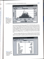
results of the simulation in the form of a frequency chart that changes as the simulations are executed. See the results ofone such run in Figure 1-9.
The frequency chart in Figure 1-9 is sometimes referred to as a risk profile. \Vhile in
this particular case our best guessof the NPV for this project would be perhaps $ 1 1,000,
we see that there is considerable uncertainty associated with the project. For example,
the frequency diagram shows the project could yield a NPV below -$9,000. At the same
time, we see that this same project could yield a NPV in excessof $30,000. As you can
see, the amount of uncertainty increasesas the width or range of the values in the frequency diagram increases.In other words, there would be less uncertainty in the NPV of
this project if the range of outcomes had been $2,000-$15,000 as opposed to the
* You may wonder why we spend time with rhis kind of detail. The reason is simple. Once you have dealt
with this kind of problem, and it is common in such analyses,you won't make this mistake in the real world where
having such errors called to your attention may be quite painful.
24.
C H A P T E R 1 / T H E WO R L D O F P R O J E C T M A N A G E MEN T
Table 1-3 Three-PointEstimateof CashFlowsand InflationRatefor psychoCeramic
Sciences,Inc.All Assumptionand ForecastCellsDefined
Year
A
2000*
Inflow
Outflow
B
c
2000
$0
0
z00L
0
2002
Net Flow
Discount
Factor
D=(B-C)
1/(1+k+p)'
$125,000 ($125,000)
1
100,000 ($1oo,ooo) 0.8696
90,000
48,333
n
($9o,ooo)
Net Present
Value
Inflation
Rate
x (Disc. Factor)
($125,000)
0.02
($86,e5i)
0.02
0.756r
($68,053)
$48,333
0.6575
$31,780
nnt
0.02
2003
117,000 15,000
$102,000
0.5718
$58,319
0.02
2004
113,333
l r L5,JJ5
0.4972
$56,347
0.02
2005
103,000
$88,000
0.4323
$38,045
0.02
2006
95,000
$95,000
0.3759
$35,714
0.02
2007
88,333
$73,333
43269
$23,973
0.02
2008
80,000
$80,000
0.2843
$22,74r
0.02
2009
63;000
34,333
$63,000
0.2472
$r),) /J
0.02
$34,333
0.2472
2009
Total
0
15,000
U
15,000
0
$742,333 $360,000
$382,333
$8,487
$10,968
*t : 0 at the beginningof2000
Formulae
CellD4
: (B4 - C4) copyto D5:D15
Cell E4
Cell E6
: U(1+ .13+ c4)^0
: U(l + .1 3+ c 5 )^ 1
: Ll(r+.13+ c 6 )^ (A 6- 999)
Cell F4
= D4*E4 copyro F5:F15
CellBlT
: Sum(B4:B15) copyto Cl Dl7, Fl7
,
Cell E5
copy ro E7:El5
range shoum in the chart thar goes ftom -9,289 to
$30,772. And as we have stated before, as the level of unceftainty increases,so does the risk.
CB provides considerable information about the forecast cell in addition
to the frequency chart including percentile information, summary statistics,
a cumulative chart,
and a reverse cumulative chart. For example, to see the ,.r*-ury statistics for
a forecast
cell, select View from the Forecast dialogne box toolbar and then select
Statistics from
the dropdown menu that appears. The Statistics view for the frequency
chart (Figure
1-9) is illustrated in Figure 1-10.
Figure 1'10 contains some interesting information. Both the mean and
median
NPV resulting from the simulation are nicely positive and thus indicate
a return above
the.hurdle rate of 13 percent (15 percent inci,rding inflation). There are,
however, several negative outcomes, those showing a return beLw the hurdle rate. li/hat
is the like-
r
I'E N T
OF RISK
1 .6 CONFRONTI NG UNCERTAI NTY- THE M A N A G E M E N T
.25
Fisure 1-9
Friquency chart of
the simulation out'
put for net present
value of PsychoCeramic Sciences,
Inc. Project.
produce a rate of relihood that this project will achieve a positive NPV, and therefore
the display shown
Using
easy.
hurdle rate? Witlr-CB, the answer is
o,
i"r"
"borr.ih.
"r
0 (or 1) in that
Type
corner.
l" pigrr" 1-9, erase -Infinity from the box in the lower left
boxes at the
The
1-11.
Figure
pr"r, Errr"r. Figure 1-9 now changesas shown in
r.)(
""a of Figrrr. 1-11 ilow that given oui estimates and assurqptions of the cash flows
bottom
project will have an NPV
and the ,ur""of inflation, there is u .qO+ probability that the
the 13 percent hurdle
above
zero and infinity, that is, a rate of return at or
f"r*".r,
rate.
in project selection
Even in this simple example the power of including uncertainty
amount of uncer'
the
should be obvious. B..u,rr" u *"tug"t is always uncertain about
quite
easily using CB'
ir-it utro possible to examine various levels of uncertainty
;i*"
,
T
I
Figure1,10 Sum'
mary statistics of
the PsychoCeramic
Sciences,Inc.
simulation.
26o
C H A P T E R 1 / T H E WO R L D O F P R O J E C T M A N A GEM EN T
Figure1.11 Calculating the probability that the net
present value of the
PsychoCeramic
Sciences,Inc. proj.
ect is equal to or
greater than the
firm's hurdle rate.
\7e could, for instance,alter the degreeto which the inflow estimates
are uncertain by
expandingor contracting the degreeto which optimistic
p"rri-oric estimatesvary
around the most likely estimat".
"nd
could increaseor decrease
the level of hflation.
Simulation runs made with these'i7.
changesprovide us with the ability to examine
irrst
how sensitivethe outcomes(forecasts) i" possibleerrorsin the input
data. This al"r. to igrror"
lows us to focuson the important risksand
thosethat have little effect on our
decisions'!7e strongly recommendthe User Manual for usersof CB (CrystatBo1@
iO;6
UserManual,2000).
THEPROJECT
PORTFOLIO
PROCESS
The Project Portfolio Process(PPP) attemptsto link rhe organization'sprojects
directly
to the goalsand strategyof,the organization.This occurs,roi orrly rn the proiecc,
irri;i;:
tion and-planning ph?:.:, but also throughout the life cycreof ihe prolects
as they are
managedand eventuallybrought to completion.Thus, the ppp is also
a"mearnfo.
itoring and controlling the organizationt strategicprojects.On occasion
-orrthis will mean
shutting down projectsprior to their completion becausetheir riskshave
becomeexcessive, their costshave escalatedbeyondtheir e*pectedbenefits,another (o,
1-r"r) proi.
ect doesa better job of supportingthe goals,oi
"
of a variety of similar reasons.
The
".ry
this processgenerallyfollow those described
in Longman,sandahl,
:!lpj^tt
sp.i,
(1999)and Englundand Graham(2000).
"rrJ
Step 1: Establish a project Council
The main purposeof the project council is to establishand articulate
a strategicdirec.
tion for projects.The council will alsobe responsiblefor allocati"g
frr"ar to ,lr-or"f.o1ectsthat supportthe organization'sgoalsand controlling the allocation
of resourcesand
skills to the projects.In addition to-senior
other appropriatemembersof
the project council includerproje.ctmanagers
-urr"g"..r.rrf,
of ilaior p-1..rr; i'lr'. head of the project
ManagementOffice (if one exists);particJarly t l"uurrig".r"rui
rhat is, those
-u.r"g.rs,
18 .
C H A P T E R 1 / T H E WO R L D O F P R O J E C T M A N A G E MEN T
l?X corurnorurruc
urucenrrurury-rne
ulrueceuerur
or nrsr
As we argue throughout this book, effective project management requires an ability to
deal with uncertainty. The time required to complete a project, the availability and
costs of key resources,the timing of solutions to technological problems, a wide variety
of macroeconomic variables, the whims of a client, the actions taken by competitors,
even the likelihood that the output of a project will perfiorm as expected, all these exemplifit the uncertainties encountered when managing projects. While there are actions
that may be taken to reduce the uncertainty, no actions of a PM can ever eliminate it.
Therefore' in today's turbulent businessenvironment, effective decision making is predicated on an ability to manage the ambiguity that arises while we operate in a world
characterized by uncertain information.
One approach that is particularly useful in helping us undersrand the implications
of uncertain information is risk utalysi.s.The essenceof risk analysis is to make estimates
or assumptions about the probability distributions associated with key parameters and
variables and to use analytic decision models or Monte Carlo simulation models based
on these distributions to evaluate the desirability of certain managerial decisions. Realworld problems are usually large enough that the use of analytic models is very difficult
and time consuming. With modern computer software, simulation is not difficult.
A mathematical model of the situation is constructed and a simulation is run to determine the model's outcomes under various scenarios, The model is run (or replicated)
repeatedly, starting from a different point each time based on random choices of values
from the probability distributions of the input variables. Outputs of the model are used
to construct statistical distributions of items of interest to decision makers, such as costs.
profits, completion dates, or retum on investment. These distributions are the risk profiles of the outcomes associated with a decision. Risk profiles can be considered by the
manager when considering a decision, along with many other factors such as strategic
concems, behavioral issues,fit with the organization, and so on.
In the following section, using an example we have examined earlier, we illustrate
ll#i;T.ik'",:ixltixi'*:
i;ifiH$:::';,'.''"T,1"'i,;*;i*:l';::1ff
ConsideringUncertaintyin Project SelectionDecisions
Reconsider the PsychoCeramic Sciences example we solved in the section devoted to
finding the discounted cash flows associatedwith a project. Setting this problem up on
Excel@ is straightforward, and the earlier solution is shown here for convenience as
Table 1'1. \ilUefound that the project cleared the barrier of a 13 percent hurdle rate for
acceptance. The net cash flow over the project's life is just under $400,000, and dis.
counted at the hurdle rate plus 2 percent annual inflation, the net present value of the
cash flow is about $18,000. The rate of inflation is shown in a separate column because
it is another uncertain variable that should be included in the risk analysis.
Assume that the expenditures in this example are fixed by contract with an outside
vendor so that there is no uncertainty about the outflows; there is, of course, uncertainty about the inflows. Suppose that the estimared inflows are as shown in Tabte 1-2
and include a minimum (pessimistic) estimate, a most likely estimate, and a maximum
(optimistic) estimate. (In Chapter 5, "scheduling the Project," we will deal in more detail with the methods and meaning of making such estimates.) Both the beta and the
triangular statistical distributions are welt suitJ for modeling variables with these three
parameters, but fitting a beta distribution is complicated and not paxricularly intuitive.
L,