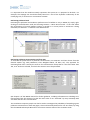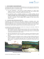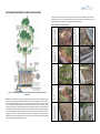
1
APPENDIX A PUBLICATIONS FAWB PUBLICATIONS Policy and Organisational Receptivity Brown, R. R. and J. M. Clarke (2007). The transition towards Water Sensitive Urban Design: The story of Melbourne. Report No. 07/01, Facility for Advancing Water Biofiltration, Monash University: 67 pp. Brown, R. R. and M. Farrelly (2007). Institutional impediments to advancing sustainable urban water management: A typology. 13th International Rainwater Catchment Systems Conference and 5th International Water Sensitive Urban Design Conference. Sydney, Australia. Brown, R. R. and J. M. Clarke (2007). The transition towards water sensitive urban design: a socio:technical analysis of Melbourne, Australia. Novatech 2007. 6th International Conference on Sustainable Techniques and Strategies in Urban Water Management. Lyon, France. 1: 349-356. Brown, R. R. and M. A. Farrelly (2007). Advancing urban stormwater quality management in Australia: A survey of stakeholder perceptions of institutional drivers and barriers. Report No. 07/05,National Urban Water Governance Program, Monash University. Available at www.urbanwatergovernance.com Filter Media Bratieres, K., T. D. Fletcher and A. Deletic (2009). The advantages and disadvantages of a sand based biofilter medium: results of a new laboratory trial. 6th International Water Sensitive Urban Design Conference and Hydropolis #3, Perth, Australia. Hatt, B. E., T. D. Fletcher and A. Deletic (2008). Hydraulic and pollutant removal performance of fine media stormwater filtration systems. Environmental Science & Technology 42(7): 2535-2541. Hatt, B. E., T. D. Fletcher and A. Deletic (2007). Stormwater reuse: designing biofiltration systems for reliable treatment. Water Science and Technology 55(4): 201-209. Hatt, B. E., T. D. Fletcher and A. Deletic (2007). The effects of drying and wetting on pollutant removal by stormwater filters. Novatech 2007. 6th International Conference on Sustainable Techniques and Strategies in Urban Water Management, Lyon, France. Hatt, B. E., T. D. Fletcher and A. Deletic (2007). Hydraulic and pollutant removal performance of stormwater filters under variable wetting and drying regimes. Water Science & Technology 56(12): 11-19. Vegetation Read, J., T. D. Fletcher, P. Wevill and A. Deletic (in press). Plant traits that enhance pollutant removal from stormwater in biofiltration systems. International Journal of Phytoremediation. Read, J., T. Wevill, T. D. Fletcher and A. Deletic (2008). Variation among plant species in pollutant removal from stormwater in biofiltration systems. Water Research 42(4-5): 893-902. Bratieres, K., T. D. Fletcher, A. Deletic and Y. Zinger (2008). Optimisation of the treatment efficiency of biofilters; results of a large-scale laboratory study. Water Research 42(14): 3930-3940. Fletcher, T. D., Y. Zinger and A. Deletic (2007). Treatment efficiency of biofilters: results of a large scale biofilter column study. 13th International Rainwater Catchment Systems Conference and 5th International Water Sensitive Urban Design Conference, Sydney, Australia. Submerged Zone Blecken, G.-T., Y. Zinger, A. Deletic, T. D. Fletcher and M. Viklander (in press). Influence of intermittent wetting and drying conditions on heavy metal removal by stormwater biofilters. Water Research. Blecken, G.-T., Y. Zinger, A. Deletic, T. D. Fletcher and M. Viklander (2009). Impact of a submerged anoxic zone and a cellulose based carbon source on heavy metal removal in stormwater biofiltration systems. Ecological Engineering 35(5): 769-778. Zinger, Y., T. D. Fletcher, A. Deletic, G. T. Blecken and M. Viklander (2007). Optimisation of the nitrogen retention capacity of stormwater biofiltration systems. Novatech 2007, 6th International Conference on Sustainable Techniques and Strategies in Urban Water Management, Lyon, France. Zinger, Y., A. Deletic and T. D. Fletcher (2007). The effect of various intermittent wet-dry cycles on nitrogen removal capacity in biofilters systems. 13th International Rainwater Catchment Systems Conference and 5th International Water Sensitive Urban Design Conference, Sydney, Australia. Hydraulic Performance Le Coustumer, S., T. D. Fletcher, A. Deletic, S. Barraud and J.F. Lewis (in press). Hydraulic performance of biofilter systems for stormwater management: influences of design and operation. Journal of Hydrology. Le Coustumer, S., T. D. Fletcher, A. Deletic and M. Potter (2008). Hydraulic performance of biofilter systems for stormwater management: lessons from a field study, Facility for Advancing Water Biofiltration and Melbourne Water Corporation (Healthy Bays and Waterways). Le Coustumer, S. and S. Barraud (2007). Long-term hydraulic and pollution retention performance of infiltration systems. Water Science and Technology 55(4): 235-243. Le Coustumer, S., T. D. Fletcher, A. Deletic and S. Barraud (2007). Hydraulic performance of biofilters: first lessons from both laboratory and field studies. Novatech 2007. 6th International Conference on Sustainable Techniques and Strategies in Urban Water Management, Lyon, France. Le Coustumer, S., T. D. Fletcher, A. Deletic and S. Barraud (2007). Hydraulic performance of biofilters for stormwater management: first lessons from both laboratory and field studies. Water Science and Technology 56(10): 93-100. Field Studies Hatt, B. E., T. D. Fletcher and A. Deletic (2009). Hydrologic and pollutant removal performance of stormwater biofiltration systems at the field scale. Journal of Hydrology 365(3-4): 310-321. Hatt, B. E., T. D. Fletcher and A. Deletic (2009). Pollutant removal performance of field-scale biofiltration systems. Water Science & Technology 59(8): 1567-1576. Hatt, B. E., T. D. Fletcher and A. Deletic (2008). Improving stormwater quality through biofiltration: Lessons from field studies. 11th International Conference on Urban Drainage. Edinburgh, UK. Lewis, J. F., B. E. Hatt, S. Le Coustumer, A. Deletic and T. D. Fletcher (2008). The impact of vegetation on the hydraulic conductivity of stormwater biofiltration systems. 11th International Conference on Urban Drainage. Edinburgh, UK. Hatt, B. E., J. Lewis, A. Deletic and T. D. Fletcher (2007). Insights from the design, construction and operation of an experimental stormwater biofiltration system. 13th International Rainwater Catchment Systems Conference and 5th International Water Sensitive Urban Design Conference, Sydney, Australia. Smith, N., R. Allen, A. McKenzie-McHarg, A. Deletic, T. D. Fletcher and B. Hatt (2007). Retrofitting functioning stormwater gardens into existing urban landscapes. Cairns International Public Works Conference, Cairns. Other Blecken, G.-T., Y. Zinger, T. M. Muthanna, A. Deletic, T. D. Fletcher and M. Viklander (2007). The influence of temperature on nutrient treatment efficiency in stormwater biofilter systems. Water Science and Technology 56(10): 83-91. Deletic, A. and G. Mudd (2006). Preliminary results from a laboratory study on the performance of bioretention systems built in Western Sydney saline soils, Facility for Advancing Water Biofiltration. APPENDIX B GUIDANCE FOR SIZING BIOFILTRATION SYSTEMS USING MUSIC IMPORTANT! This guide has been written for MUSIC v3.1 and should be used to provide appropriate modelling of biofiltration systems in MUSIC v3.1. Users should refer to the User Guide for guidance on how to model biofiltration systems (referred to as bioretention systems) in MUSIC v4. MUSIC v4 (and later versions) uses the results from FAWB’s research to take into account the design and operational factors which influence biofiltration treatment performance (e.g. filter media type and depth, presence and type of vegetation, presence and type of underdrain, presence of lining, etc.). In MUSIC v4, the user can readily model model a range of biofiltration systems, including designs with a saturated zone or a system without an underdrain (i.e., a vegetated infiltration system). Users should refer to the MUSIC User Manual for general guidance on how to model stormwater treatment systems with the MUSIC model. In particular, Chapter 3 gives step-by-step instructions on how to model treatment systems, including biofiltration systems. However, this Appendix demonstrates how MUSIC can be used to evaluate the performance of biofilters with regards to: 1. Pollutant loads 2. Pollutant concentrations 3. Flow rates 4. Runoff frequency Before using MUSIC to model proposed biofilter designers, the objectives need to be clearly defined, because the objectives will define which of these four performance measures are of primary interest. It is, however, important to note that version 3.0 of MUSIC does not account for the presence of a submerged zone at the base of the biofilter. Basic modelling process The basic parameters of the biofiltration system should be entered using the MUSIC “Bioretention” node dialogue box: Ponding depth (typically 0.1-0.3m) Area of ponded area (will be larger than filter if ponding area has sloped sides) Infiltration rate of underlying soils (0 if fully lined) Area of filter Depth of filter media (excluding drainage layer) For loamy sand, 0.45 mm is typical It is recommended to use a value 50% of the design value (ie. safety coefficient of 2) This allows a “buffer store” in the base of the system, to promote infiltration. NOTE: It does not account for a saturated zone. Length of system if overflow occurs (e.g. perimeter of overflow pit) It is important that the model accurately represents the system as it is proposed to be built. For example, the seepage rate should be ideally based on a test of the hydraulic conductivity of the underlying soils, or at least on a conservative estimate. Evaluating pollutant loads Evaluating the pollutant load reduction performance of a biofilter is easy in MUSIC, by simply rightclicking on the biofiltration node and choosing Statistics – Mean Annual Loads. In the case where the performance of several biofilters (either in parallel or in series) within a catchment is being evaluated, use Statistics – Treatment Train Effectiveness. Evaluating pollutant concentrations and flow rates To evaluate the performance of pollutant concentrations, use Statistics and then choose from the desired statistic (eg. Daily Maximum, Flow Weighted Mean, All Data, etc). The approach for evaluating flow rates is exactly the same as for concentrations except that it is the flow rather than TSS, TP or TN that is selected, for which the statistics are to be presented. See Chapter 4 of the MUSIC manual for further guidance, including information on excluding zeroflow periods from the statistics (so that the mean value is not “distorted” by many timesteps with zero flow and thus zero concentration. The Cumulative Frequency Graph can also be used to investigate the probability of exceeding a given pollutant concentration or flow rate (again, this would normally be done for non-zero flows, by using the Flow-Based Sub-Sample Bounds on the context-sensitive menu of the treatment node: 0.000 Evaluating runoff frequency Evaluation of the runoff frequency objective with MUSIC v3.0 requires the export of data into Excel for subsequent analysis. There are two basic components to the modelling: 1. Determining the pre-development runoff frequency; and 2. Modelling the post-development runoff frequency. The modelling must be done using a 6 minute timestep. The model results are then exported (at daily timestep) to Excel, to calculate the daily runoff frequency. Modelling the pre-development runoff frequency Step 1. Select or create the appropriate climate template - Select a 6 minute timestep climate template for one or more years (model should either use a single year which has been assessed as being representative of long-term climatic characteristics, or a representative five year period): Step 2. Create a pre-development source node - Create any type of source node (it could be urban, forested or agriculture – since we are only trying to model runoff, and not water quality). The node should have: 1. Appropriate rainfall-runoff properties for the location (default properties for Melbourne are given in Appendix I of the MUSIC manual) 2. A Daily Drainage Rate of 0 (since we wish to calculate the days of surface flows, and do not want MUSIC to add in baseflows) and a Daily Deep Seepage rate of 5% (highlighted): Step 3. Run model and export results - Run the model. Export the results at daily timestep, selecting only flow, and choosing the “Tab delimited” format: Step 5. Import and analyse results - Open the export file in Notepad (just double click on the created text file): - Select All and Copy Open Microsoft Excel and paste into spreadsheet - Calculate the runoff frequency (i.e., the number of days with non-zero flows) using the simple Excel functions shown below (in the case shown below (for Melbourne 1959), the natural runoff frequency is 8 days): =COUNTIF(B2:B366,0) =“COUNTIF(B2:B366, “<>0”) Modelling the post-development runoff frequency Modelling the post-development runoff frequency uses the same basic process as described for the pre-development situation. Step 1. Select or create the appropriate climate template - Select the same 6 minute timestep climate template as used for the pre-development analysis. Step 2. Create the model with impervious areas and proposed treatment systems - - Whilst you may model pervious areas for the normal MUSIC modelling (to analyse removal of TSS, TP and TN, you need only include the impervious areas when modelling runoff frequency. If you include pervious areas (with a daily baseflow rate set), they will produce baseflow, which MUSIC will interpret as contributing to daily runoff frequency; therefore, if you include pervious areas, the daily baseflow rate should be set to zero (and the daily seepage rate set to 5%, as per Step 2 for the pre-development frequency analysis. Create the network of treatment systems to retain stormwater from these impervious areas: eg. rain-garden, rainwater tank, infiltration system. The example below shows a rainwater tank being used to harvest water from a house roof, with overflow going to a rain-garden (biofiltration system). Runoff from the paved area also goes to the biofiltration system: - The design (and thus modelling) of treatment systems for reducing runoff frequency will be somewhat different to that for simply reducing pollutant loads. Systems which promote infiltration and stormwater harvesting with regular demands (eg. toilet flushing, etc.) will be most effective. For example, one solution (subject to appropriate distances to infrastructure) is to construct a biofiltration system with an unlined base, and the underdrain raised above the base, to allow water from small rainfall events to infiltrate to surrounding soils (see left-hand side diagram below with highlighted seepage loss and depth below underdrain parameters. Another option is to use no underdrain at all (having only an overflow pipe); in this case (right-hand size diagram), it can be modelled with a simple infiltration system node in MUSIC. The only ‘trick’ here is to model the extended detention depth as: Extended detention depth = ponding depth + infiltration depth x porosity. For a sandy-loam system (to support plants), the porosity 0.4. Therefore (in example below); if the ponding depth was 0.3m and the filter medium was 0.6m deep, the “depth to overflow) would be 0.3 + (0.6 x 0.4) = 0.54 m (highlighted below): Step 3. Run model and export results - Run the model. Export the results from the most downstream node (in the example above, this would be the rain-garden), at daily timestep, selecting only flow, and choosing the “Tab delimited” format. Step 4. Import and analyse results - - Follow the same steps as per the pre-development frequency; open the exported text file in Notepad, Select All and then Copy; paste into Excel, and then calculate the runoff frequency (ie. the number of days with non-zero flows. The number of days per year with non-zero flows should not be more than 15 days greater than for the pre-development case (for the example below, it is 12 days; ie. 8 + 12 = 20): =COUNTIF(B2:B366,0) =“COUNTIF(B2:B366, “<>0”) The effect of evapotranspiration in biofiltration systems MUSIC v3 does not account for the effect of evapotranspiration within a biofiltration system (raingarden), even through recent research has shown that it can result in a reduction of mean annual flow by about 30% (Hatt et al., 2009). It is hoped that version 4.0 of MUSIC will address this issue. APPENDIX C GUIDELINES FOR FILTER MEDIA IN BIOFILTRATION SYSTEMS GUIDELINES FOR FILTER MEDIA IN BIOFILTRATION SYSTEMS (Version 3.01) June 2009 The following guidelines for filter media in biofiltration systems have been prepared on behalf of the Facility for Advancing Water Biofiltration (FAWB) to assist in the development of biofiltration systems, including the planning, design, construction and operation of those systems. NOTE: This is a revision of the previous FAWB guideline specifications (published in 2006 (Version 1.01), 2008 (Version 2.01)). It attempts to provide a simpler and more robust guideline for both soilbased and engineered filter media. FAWB acknowledges the contribution of EDAW Inc., Melbourne Water Corporation, Dr Nicholas Somes (Ecodynamics), Alan Hoban (South East Queensland Healthy Waterways Partnership), Shaun Leinster (DesignFlow) and STORM Consulting to the preparation of the revised guidelines. Disclaimer The Guidelines for Soil Filter Media in Biofiltration Systems are made available and distributed solely on an "as is" basis without express or implied warranty. The entire risk as to the quality, adaptability and performance is assumed by the user. It is the responsibility of the user to make an assessment of the suitability of the guidelines for its own purposes and the guidelines are supplied on the understanding that the user will not hold EDAW Inc., Monash University, or parties to the Facility for Advancing Water Biofiltration (FAWB) (“the Licensor”) liable for any loss or damage resulting from their use. To the extent permitted by the laws of Australia, the Licensor disclaims all warranties with regard to this information, including all implied warranties of merchantability and fitness. In no event shall the Licensor be liable for any special, direct or consequential damages or any damages whatsoever resulting from loss or use, whether in action of contract, negligence or other tortious action, arising out of the use of, or performance of this information. 1 GENERAL DESCRIPTION The biofiltration filter media guidelines require three layers of media: the filter media itself (400-600 mm deep or as specified in the engineering design), a transition layer (100 mm deep), and a drainage layer (50 mm minimum cover over underdrainage pipe). The biofiltration system will operate so that water will infiltrate into the filter media and move vertically down through the profile. The filter media is required to support a range of vegetation types (from groundcovers to trees) that are adapted to freely draining soils with occasional wetting. The material should be based on natural or amended natural soils or it can be entirely engineered; in either case, it can be of siliceous or calcareous origin. In general, the media should have an appropriately high permeability under compaction and should be free of rubbish, deleterious material, toxicants, declared plants and local weeds (as listed in local guidelines/Acts), and should not be hydrophobic. The filter media should contain some organic matter for increased water holding capacity but be low in nutrient content. In the case of natural or amended natural soils, the media should be a loamy sand. Biofiltration Filter Media Guidelines (Version 3.01), Prepared by the Facility for Advancing Water Biofiltration (FAWB), June 2009. Maintaining an adequate infiltration capacity is crucial in ensuring the long-term treatment efficiency of the system. The ability of a biofiltration system to detain and infiltrate incoming stormwater is a function of the filter surface area, extended detention (ponding) depth, and the hydraulic conductivity of the filter media (Figure 1). Most importantly, design of a biofiltration system should optimize the combination of these three design elements. For a biofiltration system in a temperate climate with an extended detention depth of 100 – 300 mm and whose surface area is approximately 2% of the connected impervious area of the contributing catchment, the prescribed hydraulic conductivity will generally be between 100 – 300 mm/hr in order to meet best practice targets (Figure 2). This configuration supports plant growth without requiring too much land space. In warm, humid (sub- and dry- tropical) regions the hydraulic conductivity may need to be higher in order to achieve the required treatment performance using the same land space (i.e., ensuring that the proportion of water treated through the media meets requirements). Where one of these design elements falls outside the recommended range, the infiltration capacity can still be maintained by offsetting another of the design elements. For example, a filter media with a lower hydraulic conductivity may be used, but the surface area or the extended detention depth would need to be increased in order to maintain the treatment capacity. Similarly, if the available land were the limiting design element, the system could still treat the same size storm if a filter media with a higher hydraulic conductivity were installed. Where a hydraulic conductivity greater than 300 mm/hr is prescribed, potential issues such as higher watering requirements during the establishment should be considered. Biofiltration systems with a hydraulic conductivity greater than 600 mm/hr are unlikely to support plant growth due to poor water retention, and may also result in leaching of pollutants. However plant survival might be possible if the outlet pipe were raised to create a permanently submerged zone. filter media hydraulic conductivity conductivity extended detention depth infiltration capacity filter surface area Figure 1. Design elements that influence infiltration capacity. Biofiltration Filter Media Guidelines (Version 3.01), Prepared by the Facility for Advancing Water Biofiltration (FAWB), June 2009. Figure 2. Recommended filter media hydraulic conductivity range and potential issues The infiltration capacity of the biofiltration system will initially decline during the establishment phase as the filter media settles and compacts, but this will level out and then start to increase as the plant community establishes itself and the rooting depth increases (see Appendix A). In order to ensure that the system functions adequately at its eventual (minimum) hydraulic conductivity, a safety co-efficient of 2 should be used: i.e., designs should be modelled using half the prescribed hydraulic conductivity. If a system does not perform adequately with this hydraulic conductivity, then the area and/or ponding depth should be increased. It may also be desirable to report sensitivity to infiltration rate, rather than simply having expected rate. This is important when assessing compliance of constructed systems as systems should ideally meet best practice across a range of infiltration rates. 2 TESTING REQUIREMENTS 2.1 Determination of Hydraulic Conductivity The hydraulic conductivity of potential filter media should be measured using the ASTM F1815-06 method. This test method uses a compaction method that best represents field conditions and so provides a more realistic assessment of hydraulic conductivity than other test methods. Note: if a hydraulic conductivity lower than 100 mm/hr is prescribed, the level of compaction associated with this test method may be too severe and so underestimate the actual hydraulic conductivity of the filter media under field conditions. However, FAWB considers this to be an appropriately conservative test, and recommends its use even for low conductivity media. 2.2 Particle Size Distribution Particle size distribution (PSD) is of secondary importance compared with hydraulic conductivity. A material whose PSD falls within the following recommended range does not preclude the need for hydraulic conductivity testing i.e., it does not guarantee that the material will have a suitable hydraulic conductivity. However, the following composition range (percentage w/w) provides a useful guide for selecting an appropriate material: Biofiltration Filter Media Guidelines (Version 3.01), Prepared by the Facility for Advancing Water Biofiltration (FAWB), June 2009. Clay & Silt <3% (<0.05 mm) Very Fine Sand 5-30% (0.05-0.15 mm) Fine Sand 10-30% (0.15-0.25 mm) Medium to Coarse Sand 40-60% (0.25-1.0 mm) Coarse Sand 7-10% (1.0-2.0 mm) Fine Gravel <3% (2.0-3.4 mm) Clay and silt are important for water retention and sorption of dissolved pollutants, however they substantially reduce the hydraulic conductivity of the filter media. This size fraction also influences the structural stability of the material (through migration of particles to block small pores and/or slump). It is essential that the total clay and silt mix is less than 3% (w/w) to reduce the likelihood of structural collapse of such soils. The filter media should be well-graded i.e., it should have all particle size ranges present from the 0.075 mm to the 4.75 mm sieve (as defined by AS1289.3.6.1 - 1995). There should be no gap in the particle size grading, and the composition should not be dominated by a small particle size range. This is important for preventing structural collapse due to particle migration. 2.3 Soil-Based Filter Media: Properties The following specifications are based on results of extensive treatment performance testing conducted by FAWB as well as recommendations made by AS4419 – 2003 (Soils for Landscaping and Garden Use). Filter media must be tested for the following; media that do not meet these specifications should be rejected or amended: i. Total Nitrogen (TN) Content – <1000 mg/kg. ii. Orthophosphate (PO43-) Content – <80 mg/kg. Soils with total phosphorus concentrations >100 mg/kg should be tested for potential leaching. Where plants with moderate phosphorus sensitivity are to be used, total phosphorus concentrations should be <20 mg/kg. iii. Organic Matter Content – at least 3% (w/w). An organic content lower than 3% is likely to have too low a water holding capacity to support healthy plant growth. In order to comply with both this and the TN and PO43- content requirements, a low nutrient organic matter will be required. iv. pH – as specified for ‘natural soils and soil blends’ 5.5 – 7.5 (pH 1:5 in water). v. Electrical Conductivity (EC) – as specified for ‘natural soils and soil blends’ <1.2 dS/m. Optional testing: vi. Dispersibility – this should be carried out where it is suspected that the soil may be susceptible to structural collapse. If in doubt, then this testing should be undertaken. Potential filter media should generally be assessed by a horticulturalist to ensure that they are capable of supporting a healthy vegetation community. This assessment should take into Biofiltration Filter Media Guidelines (Version 3.01), Prepared by the Facility for Advancing Water Biofiltration (FAWB), June 2009. consideration delivery of nutrients to the system by stormwater. Any component or soil found to contain high levels of salt (as determined by EC measurements), high levels of clay or silt particles (exceeding the particle size limits set above), or any other extremes which may be considered retardant to plant growth should be rejected. 3 ENGINEERED FILTER MEDIA Where there is not a locally available soil-based material that complies with the properties outlined in Sections 2.1 - 2.3, it is possible to construct an appropriate filter medium. A washed, well-graded sand with an appropriate hydraulic conductivity should be used as the filter medium. Suitable materials include those used for the construction of turf profiles (e.g. golf greens); these materials are processed by washing to remove clay and silt fractions. In large quantities (>20 m 3), they can be obtained directly from sand suppliers, while smaller quantities can be purchased from local garden yards. The top 100 mm of the filter medium should then be ameliorated with appropriate organic matter, fertiliser and trace elements (Table 1). This amelioration is required to aid plant establishment and is designed to last four weeks; the rationale being that, beyond this point, the plants receive adequate nutrients via incoming stormwater. Table 1. Recipe for ameliorating the top 100 mm of sand filter media Constituent Granulated poultry manure fines Superphosphate Magnesium sulphate Potassium sulphate Trace Element Mix Fertilizer NPK (16.4.14) Lime 2 Quantity (kg/100 m filter area) 50 2 3 2 1 4 20 Laboratory testing has shown that biofilters that contain an engineered filter medium will achieve essentially the same hydraulic and treatment performance as those containing a soil-based filter medium (Bratieres et al., 2009). However, it is recommended that a submerged zone be included in biofiltration systems that utilise such a free draining filter medium to provide a water source for vegetation between rainfall events. 4 TRANSITION LAYER The transition layer prevents filter media from washing into the drainage layer. Transition layer material shall be a clean, well-graded sand material containing <2% fines. To avoid migration of the filter media into the transition layer, the particle size distribution of the sand should be assessed to ensure it meets ‘bridging criteria’, that is, the smallest 15% of the sand particles bridge with the largest 15% of the filter media particles (Water by Design, 2009; VicRoads, 2004): D15 (transition layer) ≤ 5 x D85 (filter media) where: D15 (transition layer) is the 15th percentile particle size in the transition layer material (i.e., 15% of the sand is smaller than D15 mm), and D85 (filter media) is the 85th percentile particle size in the filter media. Biofiltration Filter Media Guidelines (Version 3.01), Prepared by the Facility for Advancing Water Biofiltration (FAWB), June 2009. A dual-transition layer, where a fine sand overlays a medium-coarse sand, is also possible. While it is acknowledged that this can increase the complexity of the construction process, testing indicates that a dual-transition layer produces consistently lower levels of turbidity and concentrations of suspended solids in treated outflows than a single transition layer. Therefore, it is recommended that this design be specified for stormwater harvesting applications (to enable effective posttreatment disinfection) and where minimising the risk of washout during the establishment period is of particular importance. The transition layer can be omitted from a biofiltration system provided the filter media and drainage layer meet the following criteria as defined by the Victorian Roads Drainage of Subsurface Water from Roads - Technical Bulletin No 32 (VicRoads, 2004): D15 (drainage layer) ≤ 5 x D85 (filter media) D15 (drainage layer) = 5 to 20 x D15 (filter media) D50 (drainage layer < 25 x D50 (filter media) D60 (drainage layer) < 20 x D10 (drainage layer) These comparisons are best made by plotting the particle size distributions for the filter media and gravel on the same soil grading graphs and extracting the relevant diameters (Water by Design, 2009). 5 DRAINAGE LAYER The drainage layer collects treated water at the bottom of the system and converys it to the underdrain pipes. Drainage layer material is to be clean, fine gravel, such as a 2 – 5 mm washed screenings. Bridging criteria should be applied to avoid migration of the transition layer into the drainage layer (Water by Design, 2009; VicRoads, 2004): D15 (drainage layer) ≤ 5 x D85 (transition layer) where: D15 (drainage layer) is the 15th percentile particle size in the drainage layer material (i.e., 15% of the gravel is smaller than D15 mm), and D85 (transition layer) is the 85th percentile particle size in the transition layer material. Note: The perforations in the underdrain pipes should be small enough that the drainage layer cannot fall into the pipes. A useful guide is to check to that the D85 (drainage layer) is greater than the pipe perforation diameter. Geotextile fabrics are not recommended for use in biofiltration systems due to the risk of clogging. An open-weave shade cloth can be placed between the transition layer and the drainage layer to help reduce the downward migration of smaller particles if required, however this should only be adopted where there is insufficient depth for transition and drainage layers. 6 INSTALLATION It is recommended that filter media be lightly compacted during installation to prevent migration of fine particles. In small systems, a single pass with a vibrating plate should be used to compact the filter media, while in large systems, a single pass with roller machinery (e.g. a drum lawn roller) should be performed. Under no circumstance should heavy compaction or multiple-passes be made. Filter media should be installed in two lifts unless the depth is less than 500 mm. Biofiltration Filter Media Guidelines (Version 3.01), Prepared by the Facility for Advancing Water Biofiltration (FAWB), June 2009. 7 FIELD TESTING It is recommended that field testing of hydraulic conductivity be carried out at least twice: 1. one month following commencement of operation, and 2. in the second year of operation to assess the impact of vegetation on hydraulic conductivity. The hydraulic conductivity of the filter media should be checked at a minimum of three points within the system. The single ring, constant head infiltration test method (shallow test), as described by Le Coustumer et al. (2007), should be used. Given the inherent variability in hydraulic conductivity testing and the heterogeneity of the filter media, the laboratory and field results are considered comparable if they are within 50% of each other. However, even if they differ by more than 50%, the system will still function if both the field and laboratory results are within the relevant recommended range of hydraulic conductivities. REFERENCES ASTM International (2006). ASTM F 1815-06: Standard test methods for saturated hydraulic conductivity, water retention, porosity, and bulk density of putting green and sports turf root zones. West Conshohocken, U.S.A. Bratieres, K., T. D. Fletcher and A. Deletic (2009). The advantages and disadvantages of a sand based biofilter medium: results of a new laboratory trial. 6th International Water Sensitive Urban Design Conference and Hydropolis #3, Perth, Australia. Hatt, B. E., T. D. Fletcher and A. Deletic (2009). Hydrologic and pollutant removal performance of stormwater biofiltration systems at the field scale. Journal of Hydrology 365(3-4): 310-321. Le Coustumer, S., T. D. Fletcher, A. Deletic and S. Barraud (2007). Hydraulic performance of biofilters for stormwater management: first lessons from both laboratory and field studies. Water Science and Technology 56(10): 93-100. Standards Australia (1995). AS1289.3.6.1 - 1995: Methods of testing soils for engineering purposes Soil classification tests - Determination of the particle size distribution of a soil - Standard method of analysis by sieving. Sydney, Australia, Standards Australia International Ltd. Standards Australia (2003). AS4419 - 2003: Soils for landscaping and garden use. Sydney, Australia, Standards Australia International Ltd. VicRoads (2004). Drainage of Subsurface Water from Roads – Technical Bulletin No. 32. Available at: http://webapps.vicroads.vic.gov.au/vrne/vrbscat.nsf Water by Design (2009). Construction and Estabhlishment Guidelines: Swales, Bioretention Systems and Wetlands, South East Queensland Healthy Waterways Partnership, Brisbane. Biofiltration Filter Media Guidelines (Version 3.01), Prepared by the Facility for Advancing Water Biofiltration (FAWB), June 2009. APPENDIX A Figure A.1 illustrates the change in hydraulic conductivity during the establishment phase of a Melbourne biofiltration system containing a sandy loam filter media. The hydraulic conductivity initially declines as the filter media is compacted under hydraulic loading, but recovers back to the design value (as indicated by the dashed horizontal line) as plant growth and increased rooting depth counters the effects of compaction and clogging. Figure A.1 Evolution of hydraulic conductivity during the first 20 months of a biofiltration system (after Hatt et al., 2009) Biofiltration Filter Media Guidelines (Version 3.01), Prepared by the Facility for Advancing Water Biofiltration (FAWB), June 2009. APPENDIX D EXAMPLE MAINTENANCE PLAN Biofiltration Systems MAINTENANCE PLAN EXAMPLE June 2009 Table of Contents 1 2 BIOFILTRATION SYSTEM FUNCTIONS .............................................................................................. 2 MINIMISING LONGTERM MAINTENANCE ....................................................................................... 4 2.1 Filter media.............................................................................................................................. 4 2.2 Vegetation cover ..................................................................................................................... 4 2.3 Protection during construction phases ................................................................................... 4 3 ESTABLISHMENT PHASE MAINTENANCE......................................................................................... 5 3.1 Protection of filter media during construction ....................................................................... 5 3.2 Irrigation .................................................................................................................................. 6 3.3 Tree stake removal .................................................................................................................. 6 4 LONG TERM MAINTENANCE TASKS................................................................................................. 7 4.1 Schedule of visits ..................................................................................................................... 7 4.1.1 Schedule of Site Visits (Regular Inspec & Maint) ............................................................ 7 4.2 Tasks ........................................................................................................................................ 7 4.2.1 FILTER MEDIA TASKS ....................................................................................................... 7 4.2.2 HORTICULTURAL TASKS ................................................................................................... 7 4.2.3 DRAINAGE TASKS ............................................................................................................. 8 4.2.4 OTHER ROUTINE TASKS ................................................................................................... 8 4.2.5 FORM (REGULAR INSPECTION & MAINTENANCE) .......................................................... 9 5 REFERENCES .................................................................................................................................. 11 Biofiltration System Maintenance Plan - EXAMPLE i 1 BIOFILTRATION SYSTEM FUNCTIONS This is a sample maintenance plan only. When preparing a maintenance plan for a specific site, consideration should be given to the individual site requirements to ensure all the elements within a particular design are incorporated in to the plan. A sketch or drawing should be provided (as seen in Figure 1) to help maintenance personnel and asset managers understand the function and features of a particular asset. The drawing should provide enough information about the function of a system to enable appropriate management/maintenance decisions to be made. Biofiltration systems (also known as biofilters, bioretention systems and rain gardens) are designed with the primary intent of removing pollutants from stormwater before the water is discharged to the local waterway or reused for other applications (e.g. irrigation). They are typically constructed as basins, trenches or tree pits (Figure 1). Stormwater runoff generally enters the biofiltration system through a break in a standard road kerb where it temporarily ponds on the surface before slowly filtering through the soil media. Treated stormwater is then collected at the base of the biofiltration system via perforated pipes located within a gravel drainage layer before being discharged to conventional stormwater pipes or collected for reuse. Note that, in some cases, the drainage pipe is up-turned to create a permanent pool of water, or submerged zone, in the bottom of the biofiltration system. Conventional stormwater pipes also act as an overflow in most designs, taking flows that exceed the design capacity of the biofiltration system. The inclusion of biofiltration systems into the stormwater drainage system does not affect other conventional drainage elements. Stormwater discharge that exceeds the capacity of the biofiltration system may continue down the kerb to be collected in a conventional side entry pit or may overflow into a pit located within the biofiltration system that is directly connected to the conventional drainage system. Biofiltration systems provide stormwater treatment as well as landscape amenity. An additional benefit is that the passive irrigation from stormwater reduces the demand for irrigation from other sources, such as potable water. The tree and/or understorey species need to be relatively hardy, and tolerant of both freely draining sandy soils and regular inundation. The soil filter media into which the trees are planted generally has a specified hydraulic conductivity of 100 – 300 mm/hr, depending on the local climate and the configuration of the system. In the case of tree pits, the understorey (or groundcover) vegetation reduces the likelihood of clogging at the surface of the filter media. Figure 1 illustrates the intended flow pathways for stormwater through a typical biofiltration system (a tree pit, in this case) and shows some of the subsurface infrastructure that requires consideration for maintenance. Biofiltration System Maintenance Plan - EXAMPLE 2 Figure 1. Conceptual drawing of a biofiltration system illustrating stormwater flow pathways and subsurface infrastructure requiring maintenance. Biofiltration System Maintenance Plan - EXAMPLE 3 2 MINIMISING LONG-TERM MAINTENANCE Three key elements in the design and construction of raingardens and biofiltration tree pits have been identified that strongly influence the amount of long-term maintenance that is required. Adequately addressing these three key elements ensures that the long-term maintenance of these systems is predictable, and therefore minimal. The elements are: Correct filter media specification and installation; Dense vegetation cover; and Protection during construction phases. The importance of these key elements is described in more detail below. 2.1 Filter media The filter media for the biofiltration system must meet certain specifications. It is crucial that the filter media maintains its hydraulic conductivity (i.e., it’s ability to pass water through the media) in the long term. When an inappropriate filter media is installed (eg. it contains high levels of fine silt and/or clay materials), it may result in compaction or even structural collapse of the media. This leads to a substantial reduction in the treatment capacity of the system because water will not filter through the media; instead it will pond on the surface and spill out through the overflow. A symptom of this compaction is often the loss of vegetation within the biofiltration system. Similarly, filter media must be correctly installed with an appropriate level of compaction during installation. Guidelines currently recommend that filter media be lightly compacted during installation to prevent migration of fine particles. In small systems, a single pass with a vibrating plate should be used to compact the filter media, while in large systems, a single pass with roller machinery (e.g. a drum lawn roller) should be performed (FAWB, 2009). 2.2 Vegetation cover Nutrients have been identified as a key pollutant in stormwater, particularly nitrogen and phosphorus. The nutrient removal efficiency of biofiltration systems is related to the root structure and density of the plants within the system. Further, as plants mature and their roots penetrate the filter media, they play a role in maintaining the hydraulic conductivity of the media because root growth helps to maintain the surface porosity and the infiltration capacity of the filter media. As a result, it is important that dense vegetation cover is established at an early stage to prevent compaction or surface sealing. Some biofiltration tree pits are designed without understorey vegetation. In these instances, it is likely that additional maintenance will be required to maintain the porosity of the surface of the filter media (e.g. physical removal of any fine sediments that accumulate on the surface). 2.3 Protection during construction phases Protection of biofiltration systems during construction allows for good plant establishment and prevents disturbance or scour of the filter media surface. It is also important to protect the biofiltration system from heavy sediment loads, or other wash off (e.g. cement washings), during any construction in the catchment to prevent clogging of the surface of the filter media (see Section 3 for more detail). Biofiltration System Maintenance Plan - EXAMPLE 4 3 ESTABLISHMENT PHASE MAINTENANCE A number of maintenance activities have been identified that are, in most cases, only required during the establishment phase of a biofiltration system. The end of the establishment phase can be defined by the completion of both of the following: (i) The plant establishment – where plants are suitably established to no longer require irrigation and are close to their mature height and/or when larger trees no longer require tree stakes for support. This period is typically 18 to 24 months; and (ii) The biofiltration system is completely connected to its intended catchment and the catchment is no longer under construction (therefore there is less risk of high sediment loads or other contaminants, such as cement washings or fine clay sediments, being washed onto the surface of the filter media and causing clogging). It is also important that the entire catchment is connected to ensure adequate water availability for plants under normal climatic conditions. 3.1 Protection of filter media during construction Construction sites usually generate very high loads of sediment in stormwater runoff. These exceptionally high loads can cause the filter media within a biofiltration system to become clogged or blocked. Blockage may occur as a result of the accumulation of fine sediment on the surface; this can sometimes be manually removed. Accumulation of fine sediment may also occur in a layer deeper within the filter media, usually resulting in the need to remove and replace the filter media. To protect the filter media while construction activities are occurring in the catchment, at least one of the following precautions should be taken: 1. Keep the biofiltration system off-line during this period to prevent any stormwater entering – Note: adequate alternative sediment control measures must also be installed during construction to prevent heavy sediment loads being discharged directly to the stormwater system while the biofiltration system is off-line; 2. Delay final landscaping and protect the system by covering the entire biofiltration surface with geotextile (and turf or gravel if desired for aesthetic purposes) as shown in Figure 2 (left); or 3. Temporarily partition the biofiltration system, creating a sacrificial sediment forebay. This allows the vegetation to establish in the rest of the system while the sacrificial sediment forebay at the inlet is protected using textile and turf, as described above and shown in Figure 2 (right). This approach is best suited when the overflow pit is located close to the inlet zone. Figure 2. Protection of filter media with a geofabric and turf cover (left) and use of a sacrificial sediment forebay during construction and plant establishment (right). Biofiltration System Maintenance Plan - EXAMPLE 5 3.2 Irrigation Plants and trees in biofiltration systems will probably require irrigation during the establishment phase. Irrigation should be applied directly to the surface of the filter media. The use of Ag pipes for irrigating young trees is not recommended as it creates a short-circuit pathway, or preferential flow path, for stormwater. The stormwater flows straight down the Ag pipes and into the drainage layer at the base where it is conveyed downstream to the conventional stormwater system, effectively bypassing any pollutant removal processes that occur as the stormwater filters through the filter media (Figure 3). Figure 3. Concept illustration showing how Ag pipes installed for tree watering can result in short-circuiting and reduced stormwater treatment. 3.3 Tree stake removal Tree stakes are often used to support young trees planted into the filter media of biofiltration systems. The stakes should be removed once the trees are adequately established and the holes filled in with filter media. Failure to fill in the holes will result in the creation of a short-circuit pathway, or preferential flow path, for stormwater. Instead of ponding on the surface of the raingarden, the holes left behind after the stakes are removed allow water to bypass the filter media and drain directly into the drainage layer at the base of the cell, effectively bypassing any pollutant removal processes. Biofiltration System Maintenance Plan - EXAMPLE 6 4 4.1 4.1.1 LONG-TERM MAINTENANCE TASKS Schedule of visits Schedule of Site Visits (Regular Inspection & Maintenance) Purpose of visit Frequency Inspection Regular inspection and maintenance should be carried out to ensure the system functions as designed. It is recommended that these checks be undertaken on a three monthly basis during the initial period of operating the system. A less frequent schedule might be determined after the system has established. Maintenance 4.2 Tasks The scope of maintenance tasks should include verifying the function and condition of the following elements: Filter media Horticultural Drainage infrastructure Other routine tasks 4.2.1 FILTER MEDIA TASKS Sediment deposition Remove sediment build up from forebays and other pre-treatment measures in biofiltration systems and from the surface of biofiltration street trees. Frequency - 3 MONTHLY, AFTER RAIN Holes or scour Infill any holes in the filter media. Check for erosion or scour and repair, provide energy dissipation (e.g. rocks and pebbles at inlet) if necessary. Frequency - 3 MONTHLY, AFTER RAIN Filter media surface porosity Inspect for the accumulation of an impermeable layer (such as oily or clayey sediment) that may have formed on the surface of the filter media. A symptom may be that water remains ponded in the biofiltration system for more than a few hours after a rain event. Repair minor accumulations by raking away any mulch on the surface and scarifying the surface of the filter media between plants. For biofiltration tree pits without understorey vegetation, any accumulation of leaf litter should be removed to help maintain the surface porosity of the filter media. Frequency - 3 MONTHLY, AFTER RAIN Litter control Check for litter (including organic litter) in and around treatment areas. Remove both organic and anthropogenic litter to ensure flow paths and infiltration through the filter media are not hindered. Frequency - 3 MONTHLY OR AS DESIRED FOR AESTHETICS 4.2.2 HORTICULTURAL TASKS Pests and diseases Assess plants for disease, pest infection, stunted growth or senescent plants. Treat or replace as necessary. Reduced plant density reduces pollutant removal and infiltration performance. Frequency - 3 MONTHLY OR AS DESIRED FOR AESTHETICS Maintain original plant Infill planting: Between 6 and 10 plants per square metre should (depending on species) be adequate to maintain a density where the plants’ roots touch each other. Biofiltration System Maintenance Plan - EXAMPLE 7 densities Planting should be evenly spaced to help prevent scouring due to a concentration of flow. Frequency - 3 MONTHLY OR AS DESIRED FOR AESTHETICS Weeds It is important to identify the presence of any rapidly spreading weeds as they occur. The presence of such weeds can reduce dominant species distributions and diminish aesthetics. Weed species can also compromise the systems long term performance. Inspect for and manually remove weed species. Application of herbicide should be limited to a wand or restrictive spot spraying due to the fact that rain gardens and biofiltration tree pits are directly connected to the stormwater system. Frequency - 3 MONTHLY OR AS DESIRED FOR AESTHETICS 4.2.3 DRAINAGE TASKS Underdrain Ensure that underdrain pipes are not blocked to prevent filter media and plants from becoming waterlogged. If a submerged zone is included, check that the water level is at the design level, noting that drawdown during dry periods is expected. A small steady clear flow of water may be observed discharging from the underdrain at its connection into the downstream pit some hours after rainfall. Note that smaller rainfall events after dry weather may be completely absorbed by the filter media and not result in flow. Remote camera (eg. CCTV) inspection of pipelines for blockage and structural integrity could be useful. Frequency - 6 MONTHLY, AFTER RAIN High flow inlet pits, overflow pits and other stormwater junction pits Ensure inflow areas and grates over pits are clear of litter and debris and in good and safe condition. A blocked grate would cause nuisance flooding. Inspect for dislodged or damaged pit covers and ensure general structural integrity. Remove sediment from pits and entry sites, etc. (likely to be an irregular occurrence in mature catchment). Frequency - MONTHLY AND OCCASIONALLY AFTER RAIN 4.2.4 OTHER ROUTINE TASKS Inspection after rainfall Occasionally observe biofiltration system after a rainfall event to check infiltration. Identify signs of poor drainage (extended ponding on the filter media surface). If poor drainage is identified, check land use and assess whether it has altered from the design capacity (eg. unusually high sediment loads may require installation of a sediment forebay). Frequency – TWICE A YEAR, AFTER RAIN Biofiltration System Maintenance Plan - EXAMPLE 8 4.2.5 FORM (REGULAR INSPECTION & MAINTENANCE) Location Raingarden/Tree Pit Site Visit Date: Site Visit By: Weather: Routine Inspection Complete section 1 (below) Routine Maintenance Complete sections 1 and 2 (below) Purpose of the Site Visit NOTE: Where maintenance is required (‘yes’ in Section 2), details should be recorded in the ‘Additional Comments’ section at the end of this document. 1. Filter media *In addition to regular inspections, it is recommended that inspection for damage and blockage is made after significant rainfall events that might occur once or twice a year. Section 1 Section 2 Maintenance Required? Yes No Maintenance Performed Yes No Filter media (CIRCLE – pooling water/accumulation of silt & clay layer/scour/holes/sediment build up) Litter (CIRCLE - large debris/accumulated vegetation/anthropogenic) Vegetation health (CIRCLE - signs of disease/pests/poor growth) Vegetation densities (CIRCLE – low densities- infill planting required) Build up of organic matter, leaf litter (CIRCLE - requires removal) Weeds (CIRCLE - isolated plants/infestation) (SPECIES - …………………………………………………………….) 2. Vegetation Biofiltration System Maintenance Plan - EXAMPLE 9 3. Pits, pipes and inflow areas Section 1 Section 2 Maintenance Required? Yes No Maintenance Performed? Yes No Perforated pipes (CIRCLE – full blockage/partial blockage/damage) Inflow areas (CIRCLE – scour/excessive sediment deposition/litter blockage) Overflow grates (CIRCLE – damage/scour/blockage) Pits (CIRCLE – poor general integrity/sediment build-up/litter/blockage) Other stormwater pipes and junction pits (CIRCLE – poor general integrity/sediment build-up/litter/blockage) 4. Submerged zone Section 1 Section 2 Maintenance Required? Yes No Maintenance Performed? Yes No Weir/up-turned pipe (CIRCLE – full blockage/partial blockage/damage) Water level (CIRCLE – at design level/drawn down) SOME DRAWDOWN DURING DRY PERIODS IS EXPECTED 5. Additional Comments Biofiltration System Maintenance Plan - EXAMPLE 10 5 REFERENCES FAWB (2009). Guidelines for Filter Media in Biofiltration Systems (Version 3.01), Facility for Advancing Water Biofiltration, available at http://www.monash.edu.au/fawb/publications Biofiltration System Maintenance Plan - EXAMPLE 11 APPENDIX E PRACTICE NOTE 1: IN SITU MONITORING OF HYDRAULIC CONDUCTIVITY CONDITION ASSESSMENT AND PERFORMANCE EVALUATION OF BIOFILTRATION SYSTEMS PRACTICE NOTE 1: In Situ Measurement of Hydraulic Conductivity Belinda Hatt, Sebastien Le Coustumer June 2009 The Facility for Advancing Water Biofiltration (FAWB) aims to deliver its research findings in a variety of forms in order to facilitate widespread and successful implementation of biofiltration technologies. This Practice Note for In Situ Measurement of Hydraulic Conductivity is the first in a series of Practice Notes being developed to assist practitioners with the assessment of construction and operation of biofiltration systems. Disclaimer: Information contained in this Practice Note is believed to be correct at the time of publication, however neither the Facility for Advancing Water Bioifltration nor its industry partners accept liability for any loss or damage resulting from its use. 1. SCOPE OF THE DOCUMENT This Practice Note for In Situ Measurement of Hydraulic Conductivity is designed to complement FAWB’s Guidelines for Filter Media in Biofiltration Systems, Version 3.01 (visit http://www.monash.edu.au/fawb/publications/index.html for a copy of these guidelines). However, the recommendations contained within this document are more widely applicable to assessing the hydraulic conductivity of filter media in existing biofiltration systems. For new systems, this Practice Note does not remove the need to conduct laboratory testing of filter media prior to installation. 2. DETERMINATION OF HYDRAULIC CONDUCTIVITY The recommended method for determining in situ hydraulic conductivity uses a single ring infiltrometer under constant head. The single ring infiltrometer consists of a small plastic or metal ring that is driven 50 mm into the filter media. It is a constant head test that is conducted for two different pressure heads (50 mm and 150 mm). The head is kept constant during all the experiments by pouring water into the ring. The frequency of readings of the volume poured depends on the filter media, but typically varies from 30 seconds to 5 minutes. The experiment is stopped when the infiltration rate is considered steady (i.e., when the volume poured per time interval remains constant for at least 30 minutes). This method has been used extensively (eg. Reynolds and Elrick, 1990; Youngs et al., 1993). Note: This method measures the hydraulic conductivity at the surface of the filter media. In most cases, it is this top layer which controls the hydraulic conductivity of the system as a whole (i.e., the underlying drainage layer has a flow capacity several orders of magnitude higher than the filter media), as it is this layer where fine sediment will generally be deposited to form a “clogging layer”. However this shallow test would not be appropriate for systems where the controlling layer is not 1 the surface layer (eg. where migration of fine material down through the filter media has caused clogging within the media). In this case, a ‘deep ring’ method is required; for further information on this method, see Le Coustumer et al. (2008). 2.1 Selection of monitoring points For biofiltration systems with a surface area less than 50 m2, in situ hydraulic conductivity testing should be conducted at three points that are spatially distributed (Figure 1). For systems with a surface area greater than 50 m2,an extra monitoring point should be added for every additional 100 m2. It is essential that the monitoring point is flat and level. Vegetation should not be included in monitoring points. Figure 1. Spatially distributed monitoring points. 2.2 Apparatus The following is required: 100 mm diameter PVC rings with a height of at least 220 mm – the bottom edge of the ring should be bevelled and the inside of the ring should be marked to indicate 50 mm and 150 mm above the filter media surface (Figure 2) 40 L water 100 mL, 250 mL and 1000 mL measuring cylinders Stopwatch Thermometer Measuring tape Spirit level 2 Hammer Block of wood, approximately 200 x 200 mm Figure 2. Diagram of single ring infiltrometer. 2.3 Procedure a. Carefully scrape away any surface covering (eg. mulch, gravel, leaves) without disturbing the soil filter media surface (Figure 3b). b. Place the ring on the surface of the soil (Figure 3c), and then place the block of wood on top of the ring. Gently tap with the hammer to drive the ring 50 mm into the filter media (Figure 3d). Use the spirit level to check that the ring is level. Note: It is essential that this the ring is driven in slowly and carefully to minimise disturbance of the filter media profile. c. Record the initial water temperature. d. Fill the 1000 mL measuring cylinder. e. Using a different pouring apparatus, slowly fill the ring to a ponding depth of 50 mm, taking care to minimise disturbance of the soil surface (Figure 3f). Start the stopwatch when the water level reaches 50 mm. f. Using the 1000 mL measuring cylinder, maintain the water level at 50 mm (Figure 3g). After 30 seconds, record the volume poured. g. Maintain the water level at 50 mm, recording the time interval and volume required to do so. Note: The time interval between recordings will be determined by the infiltration capacity of the filter media. For fast draining media, the time interval should not be greater than one minute however, for slow draining media, the time between recordings may be up to five minutes. 3 Note: The smallest measuring cylinder that can pour the volume required to maintain a constant water level for the measured time interval should be used for greater accuracy. For example, if the volume poured over one minute is 750 mL, then the 1000 mL measuring cylinder should be used. Similarly, if the volume poured is 50 mL, then the 100 mL measuring cylinder should be used. h. Continue to repeat Step f until the infiltration rate is steady i.e., the volume poured per time interval remains constant for at least 30 minutes. i. Fill the ring to a ponding depth of 150 mm (Figure 3h). Restart the stopwatch. Repeat steps e – g for this ponding depth. Note: Since the filter media is already saturated, the time required to reach steady infiltration should be less than for the first ponding depth. j. Record the final water temperature. k. Enter the temperature, time, and volume data into a calculation spreadsheet (see “Practice Note 1_Single Ring Infiltration Test_Example Calculations.xls”, available at www.monash.edu.au/fawb/publications/index.html, as an example). 2.4 Calculations In order to calculate Kfs a ‘Gardner’s’ behaviour for the soil should be assumed (Gardner, 1958 in Youngs et al., 1993): K(h) K fs e αh Eqn. 1 where K is the hydraulic conductivity, α is a soil pore structure parameter (large for sands and small for clay), and h is the negative pressure head. Kfs is then found using the following analytical expression (for a steady flow) (Reynolds and Elrick, 1990): K fs G Q2 a H2 Q1 H1 Eqn. 2 where a is the ring radius, H1 and H2 are the first (50 mm) and second (150 mm) pressure heads, respectively, Q1 and Q2 are the steady flows for the first and second pressure heads, respectively, and G is a shape factor estimated as: G 0.316 d a 0.184 Eqn. 3 where d is the depth of insertion of the ring and a is the ring radius. G is nearly independent of soil hydraulic conductivity (i.e., Kfs and α) and ponding, if the ponding is greater than 50 mm. 4 a b c d e f g h Figure 3. Measuring hydraulic conductivity. 5 The possible limitations of the test are (Reynolds et al., 2000): (1) the relatively small sample size due to the size of the ring, (2) soil disturbance during installation of the ring (compaction of the soil), and (3) possible edge flow during the experiments. 3 INTERPRETATION OF RESULTS This test method has been shown to be relatively comparable to laboratory test methods (Le Coustumer et al., 2008), taking into account the inherent variability in hydraulic conductivity testing and the heterogeneity of natural soil-based filter media. While correlation between the two test methods is low, results are not statistically different. In light of this, laboratory and field results are deemed comparable if they are within 50% of each other. In the same way, replicate field results are considered comparable if they differ by less than 50%. Where this is not the case, this is likely to be due to a localised inconsistency in the filter media, therefore additional measurements should be conducted at different monitoring points until comparable results are achieved. If this is not achieved, then an area-weighted average value may need to be calculated. 4 MONITORING FREQUENCY Field testing of hydraulic conductivity should be carried out at least twice: (1) One month following commencement of operation, and (2) In the second year of operation to assess the impact of vegetation on hydraulic conductivity. Following this, hydraulic conductivity testing should be conducted every two years or when there has been a significant change in catchment characteristics (eg. construction without appropriate sediment control). REFERENCES Gardner, W. R. (1958). Some steady-state solutions of the unsaturated moisture flow equation with application to evaporation from a water table. Soil Science 85: 228-232. Le Coustumer, S., T. D. Fletcher, A. Deletic and M. Potter (2008). Hydraulic performance of biofilter systems for stormwater management: lessons from a field study, Melbourne Water Corporation, available at: www.monash.edu.au/fawb/publications Reynolds, W. D., B. T. Bowman, R. R. Brunke, C. F. Drury and C. S. Tan (2000). Comparison of tension infiltrometer, pressure infiltrometer, and soil core estimates of saturated hydraulic conductivity. Soil Science Society of America journal 64(2): 478-484. Reynolds, W. D. and D. E. Elrick (1990). Ponded infiltration from a single ring: Analysis of steady flow. Soil Science Society of America journal 54: 1233-1241. Youngs, E. G., D. E. Elrick and W. D. Reynolds (1993). Comparison of steady flows from infiltration rings in "Green and Ampt" and "Gardner" soils. Water Resources Research 29(6): 1647-1650. 6 Single Ring Infiltration Test Site: _____________________________________________ Date: _____________________________________________ Constant water level = 50 mm Constant water level = 150 mm Time (min) Time (min) Volume (mL) Q (mL/s) Volume (mL) Q (mL/s) APPENDIX F PRACTICE NOTE 2: PREPARATION OF SEMI-SYNTHETIC STORMWATER CONDITION ASSESSMENT AND PERFORMANCE EVALUATION OF BIOFILTRATION SYSTEMS PRACTICE NOTE 2: Preparation of Semi-Synthetic Stormwater Belinda Hatt and Peter Poelsma February 2009 The Facility for Advancing Water Biofiltration (FAWB) aims to deliver its research findings in a variety of forms in order to facilitate widespread and successful implementation of biofiltration technologies. This Practice Note for Preparation of Semi-Synthetic Stormwater is part of a series of Practice Notes being developed to assist practitioners with assessing the performance of biofiltration systems. Disclaimer: Information contained in this Practice Note is believed to be correct at the time of publication, however neither the Facility for Advancing Water Bioifltration nor its industry partners accept liability for any loss or damage resulting from its use. 1. SCOPE OF THE DOCUMENT This Practice Note for Preparation of Semi-Synthetic Stormwater is designed to complement FAWB’s Performance Assessment of Biofiltration Systems using Simulated Rain Events. Semi-synthetic stormwater is also appropriate for laboratory-scale testing of biofiltration and other stormwater treatment systems (eg. porous pavements, constructed wetlands). 2. INTRODUCTION There are advantages and disadvantages to using either “natural” or “synthetic” stormwater for performance assessment. The advantage of using natural stormwater (i.e., stormwater collected from a drainage outlet) is that the physical, chemical and biological characteristics will be truly representative of real stormwater. However, the disadvantage is that maintaining consistency of concentration and characteristics (eg. sediment particle size distribution (PSD)) will be very difficult, potentially introducing an artefact of inflow variations into the measurement of treatment performance. Collection of natural stormwater can be logistically difficult and is dependent on rain events, an almost certain complication to any monitoring program. The advantage of using synthetic (i.e., using laboratory chemicals) stormwater is that is readily available and will better achieve consistency, however it will introduce artefacts due to unnatural composition (Deletic & Fletcher, 2006). Semi-synthetic stormwater represents an appropriate compromise because it is prepared using sediment sourced from a stormwater pond. Since it is actual stormwater sediment, this should also largely achieve desired nutrient and heavy metal concentrations; any deficiencies can then be topped up using laboratory-grade chemicals. 3. METHODOLOGY The basic procedure in preparing semi-synthetic stormwater is to collect sediment from a stormwater pond, prepare a slurry of known sediment concentration, mix this with dechlorinated 1 water1 and add laboratory-grade chemicals as required. The first time sediment is collected, pilot study-type testing of the slurry needs to be conducted to characterise the sediment (pollutant concentration, PSD, as described in Section 3.3.3). For subsequent collections, only the sediment concentration of the slurry needs to be tested. 3.1 Target characteristics 3.1.1 Pollutant concentrations There is a high level of spatial and temporal variability in stormwater pollutant concentrations. Where local stormwater quality data is available, these should be the target pollutant concentrations. However, where such data is not available, typical pollutant concentrations for runoff from urban areas would be appropriate targets (Table 1). Table 1. Typical stormwater pollutant concentrations (Duncan, 1999; Taylor et al., 2005). Pollutant Total Suspended Solids (TSS) Total Nitrogen (TN) Nitrate/Nitrite (NOx) Ammonia (NH3) Dissolved Organic Nitrogen (DON) Particulate Organic Nitrogen (PON) Total Phosphorus (TP) Filterable Reactive Phosphorus (FRP) Cadmium (Cd) Chromium (Cr) Copper (Cu) Lead (Pb) Manganese (Mn) Nickel (Ni) Zinc (Zn) Total Petroleum Hydrocarbons (TPH) + Polyaromatic Hydrocarbons (PAH) Concentration (mg/L) 150 2.2 0.74 0.34 0.69 0.50 0.35 0.12 0.0045 0.025 0.05 0.14 0.23 0.031 0.25 10 The list of stormwater pollutants presented in Table 1 is by no means exhaustive, however these are the pollutants that are of most concern where the management objective is protection of aquatic ecosystems. It may not be possible to analyse for all of these pollutants, depending on the available budget, however the minimum suite of pollutants should include TSS, TN, TP, Cd, Cu, Pb, Zn. If reuse is planned, pathogens are a key water quality issue and should be considered as an additional pollutant. 3.1.2 Particle size distribution The PSD of stormwater sediment varies widely according to catchment characteristics, as well as rainfall patterns and intensity. Like pollutant concentrations, local information should form the basis 1 Mains or recycled water is suitable 2 of appropriate targets, however where this data does not exist, it would be appropriate to aim for a median particle size (d50) of 25 - 60 μm (Siriwardene et al., 2007). Note: Given the large spatial and temporal variation in PSDs, it is neither feasible nor justified to try to match an exact PSD. However, many stormwater pollutants are known to attach to very small particles (eg. heavy metals are strongly correlated to particles that are <15 μm, Sansalone & Buchberger, 1995), therefore it should be ensured that this fraction is adequately represented (5 – 15 % of weight fraction). 3.2 Collection of stormwater sediment Collect sediment from near (but a short distance from) the inlet of a stormwater pond or wetland using a shovel; sediment very close to the inlet is dominated by coarse sand and gravel. Slowly scrape the surface of the sediment layer (this is the “freshest” sediment i.e., it has most recently been stormwater), taking care to minimise disturbance. The amount of sediment that needs to be collected will depend on the volume of stormwater to be prepared; as a general guide, 5 L of sediment will make 3000 L of semi-synthetic stormwater. 3.3 Preparation and analysis of sediment slurry A slurry is a concentrated mixture of sediment and water. This is prepared by wet sieving the sediment using a small volume of water. 3.3.1 Apparatus The following apparatus is required: Scoop Sieve (see below for guidance on appropriate size) Collection vessel Small cup or beaker Spatula or rubber squeegee Water Biofilters (and other stormwater treatment structures) may or may not incorporate pre-treatment. Where systems do not have pre-treatment facilities, a 1 mm sieve should be used to remove very large particles, while a 300 μm sieve should be used for systems that do have pre-treatment. The aim of this procedure is to try to replicate the realistic nature of the inflow sediment that will enter the biofiltration system in operation. Caution: Stormwater sediment potentially contains pathogens and, while the risk of falling ill is low, appropriate protocols for safe-handling of environmental samples should be followed, including long gloves, covered skin, and safety glasses. Personnel should also have received necessary vaccinations; consult a general practitioner or health advisor for further information. 3.3.2 Procedure a. Place the sieve on top of the collection vessel 3 b. Place several scoops of sediment on the sieve c. Pour a cup of water over the sediment d. Use spatula or squeegee to stir sediment around, allowing water to wash particles through to the collection chamber e. Wash and stir the sediment in the sieve with ten cups of water, then discard the fraction that did not pass through the sieve Note: When all the clean water has washed through the sieve, use the cup to scoop up supernatent liquid from the collection vessel (avoid scooping up settled sediment) and use this liquid to wash the sediment in the sieve, stirring with the spatula while doing so. f. Repeat Steps b to e until the required volume of slurry (plus some extra for analysis) has been prepared. 3.3.3 Analysis The first time sediment is collected from a stormwater pond, all of the tests described below must be carried out in order to characterise the sediment. For subsequent collections, only the sediment concentration of the slurry needs to be analysed, provided that inflow samples of the stormwater are collected during testing. Sediment concentration. The method for measuring the sediment concentration of the slurry is an adaptation of the Australian Standard method for determination of total solids in waters (Australian Standard, 1990). Rapidly stir the slurry so that all particles are in suspension and immediately collect three 100 mL samples of the slurry (continue stirring between each sample collection), transfer each sample to a pre-weighed container, and dry in an oven at 105⁰ for one hour. Allow the containers to cool at room temperature before weighing again. Calculate the sediment concentration of each sample using Equation 1 and determine the average. cs mc mc s v Equation 1 where: cs = sediment concentration in slurry (mg/L) mc+s = dry mass of container + slurry (mg) mc = mass of container (mg) v = volume of slurry (0.1 L) Note: The target sediment concentration should be around 300 ± 200 g/L. Particle size distribution. There is a high level of uncertainty associated with measurement of the PSD, and low levels of agreement between test methods. Consistently using the same test method is therefore more important than the actual test method. PSD is typically measured using sieving techniques or particle sizers; given that both methods have their advantages and disadvantages, it is recommended that the test method that is most readily available and convenient be adopted, and then used consistently for all subsequent tests. 4 Pollutant concentration. A sub-sample of the slurry should be mixed with water to achieve the target TSS concentration; see Section 3.5 for guidance on calculating the required volumes. A sample of this should then be analysed for all the pollutants of interest by a NATA-accredited laboratory. 3.4 Addition of laboratory grade chemicals Once the pollutant concentration of the slurry/water mix has been determined, the need for “topping up” pollutant concentrations can be assessed. Where this is required, laboratory grade chemicals should be used. The chemicals that should be used for each pollutant are listed in Table 2; see Section 3.5 for guidance on calculating the required amount to add. Table 2. Chemicals for topping up stormwater pollutant concentrations. Note that it is important to use these particular chemicals due to solubility considerations e.g. Lead (Pb) forms an insoluble salt with sulphate (SO4) and chloride (Cl). Pollutant TN NOx NH3 DON PON TP FRP Cd Cr Cu Pb Mn Ni Zn TPH & PAH Compound to dose with n/a* potassium nitrate (KNO3) ammonium chloride (NH4Cl) nicotonic acid (C6H5O2N) n/a† n/a† potassium phosphate (KH2PO4) 1000 mg/L standard solution chromium nitrate (Cr(NO3)3) copper sulphate (CuSO4) lead nitrate (Pb(NO3)2) manganese nitrate (Mn(NO3)2) nickel nitrate (Ni(NO3)2) zinc chloride (ZnCl2) diesel *TN is the sum of NOx, NH3, DON and PON; if the targets concentrations of these constituents are met, then the target TN concentration will also be achieved. † PON is sourced from the slurry, while TP is the sum of particulate phosphorus sourced from the slurry and FRP. Caution: Aquire and observe the Material Safety Data Sheets (MSDS) for each chemical that is used and follow appropriate protocols for safe handling and storage of chemicals. 3.5 Preparation of stormwater Sections 3.5.1 – 3.5.3 describe the calculations required to determine to final volumes. The spreadsheet “Practice Note 2_Preparation of semi-synthetic stormwater_dosing calculations.xls”, available at http://www.monash.edu.au/fawb/products/index.html, can also be used to calculate the required mass of chemicals and slurry needed to prepare the semi-synthetic stormwater. 3.5.1 Dechlorinated water Mains water generally contains residual chlorine, which should be neutralised with sodium thiosulphate (Na2S2O3) prior to preparing the semi-synthetic stormwater (to avoid it having an effect 5 on the biological community in the biofilter). The amount of sodium thiosulphate to add: 0.1 g/100 L water. 3.5.2 Amount of slurry to add The amount of slurry to add is calculated using Equation 2: vs = TSS × v st cs Equation 2 where: vs = volume slurry (L) TSS = target TSS concentration (mg/L) vst = volume semi-synethic stormwater (L) cs = sediment concentration in slurry (mg/L) 3.5.3 Mass of chemicals to add The amount of chemical to add is calculated by substracting the concentration achieved by adding the slurry from the target concentration and converting the difference to a mass (Equation 3). Since the concentration is reported as mg/L of the pollutant of interest (e.g. Cu), the calculation includes a conversion from the mass of that pollutant to the equivalent mass of the compound (e.g. CuSO4). m (dosing compound)= (c t - c sw) × v st × 1 Mr(pollutant of interest) Mr(dosing compound) Equation 3 where: m(dosing compound) = mass of dosing compound (mg) ct = target pollutant concentration (mg/L) csw = pollutant concentration achieved by slurry/water mix (mg/L) vst = volume semi-synthetic stormwater (mg/L) Mr(pollutant of interest) = molecular mass of pollutant of interest (g/mol) Mr(dosing compound) = molecular mass of dosing compound (g/mol) For example, the target concentration for Cu is 0.05 mg/L, however a slurry prepared from sediment Wetland A and mixed with water to the target TSS concentration only has a Cu concentration of 0.01 mg/L. Therefore, the concentration needs to be increased by 0.04 mg/L. The molecular mass of Cu is 63.55 g/mol, while that of CuSO4 is 159.62 g/mol. To prepare 600 L of semi-synthetic stormwater that meets the target Cu concentration, 0.06 g of CuSO4 needs to be added to the slurry/water mix. 6 m(CuSO 4)=(0. 05 - 0 .01)× 600 × 3.5.4 1 63.55 159.62 = 60mg = 0.06 g Mixing the semi-synthetic water The water, slurry and chemicals (as required) should be mixed in a tank and stirred continuously (this can be mechanical or manual). It is important that the stormwater is mixed for at least ten minutes to allow for the adsorption of various pollutants to particles in the mixture - the proportion of dissolved and particulate pollutants has a major influence on treatment performance. Slurry can be prepared and kept for several weeks, if refrigerated in a container with a secure lid (to reduce evaporation), however stormwater should be used on the day it is prepared. REFERENCES Australian Standard (1990). AS 3550.4-1990 Waters - Part 4: Determination of solids - Gravimetric method. Homebush, New South Wales, Standards Australia. Deletic, A. and T. D. Fletcher (2006). Performance of grass filters used for stormwater treatment - a field and modelling study. Journal of Hydrology 317(3-4): 261-275. Duncan, H. P. (1999). Urban Stormwater Quality: A Statistical Overview. Melbourne, Australia, Cooperative Research Centre for Catchment Hydrology: 80. Sansalone, J. J. and S. G. Buchberger (1995). An infiltration device as a best management practice for immobilizing heavy metals in urban highway runoff. Water Science and Technology 32(1): 119-125. Siriwardene, N. R., A. Deletic and T. D. Fletcher (2007). Clogging of stormwater gravel infiltration systems and filters: insights from a laboratory study. Water Research 41(7): 1433-1440. Taylor, G. D., T. D. Fletcher, T. H. F. Wong, P. F. Breen and H. P. Duncan (2005). Nitrogen composition in urban runoff - implications for stormwater management. Water Research 39(10): 1982-1989. 7 APPENDIX G PRACTICE NOTE 3: PERFORMANCE ASSESSMENT OF BIOFILTRATION SYSTEMS USING SIMULATED RAIN EVENTS CONDITION ASSESSMENT AND PERFORMANCE EVALUATION OF BIOFILTRATION SYSTEMS PRACTICE NOTE 3: Performance Assessment of Biofiltration Systems using Simulated Rain Events Belinda Hatt March 2009 The Facility for Advancing Water Biofiltration (FAWB) aims to deliver its research findings in a variety of forms in order to facilitate widespread and successful implementation of biofiltration technologies. This Practice Note for Performance Assessment of Biofiltration Systems using Simulated Rain Events is part of a series of Practice Notes being developed to assist practitioners with the assessment of construction and operation of biofiltration systems. Disclaimer: Information contained in this Practice Note is believed to be correct at the time of publication, however neither the Facility for Advancing Water Bioifltration nor its industry partners accept liability for any loss or damage resulting from its use. 1. SCOPE OF THE DOCUMENT This Practice Note for Performance Assessment of Biofiltration Systems using Simulated Rain Events is designed to provide practitioners with a hydrologic and treatment performance assessment tool where a more detailed assessment than collecting the occasional water quality sample is required, but where continuous flow and water quality monitoring is not feasible. From a practical viewpoint, this approach is limited to small-scale systems as the volume of stormwater required to evaluate large-scale systems is too onerous. This approach is also limited to sites where the outlet can be easily accessed in order to measure flow and collect water quality samples. 2. RAIN EVENT SIMULATION The hydrologic and treatment performance of biofiltration systems can be assessed by simulating a rain event. A pre-determined volume of semi-synthetic water (usually equivalent to that of the design storm) is prepared and delivered to the biofiltration system. Normally this is done via a tanker truck and a mixing tank. The outflow rate is measured and water quality samples are collected at regular intervals until outflow ceases. Simulating a rain event is a full-day exercise and initially requires a minimum number of four people; the busiest stage is preparing and delivering the semi-synthetic stormwater to the biofilter. Once this stage has finished, two people can manage the flow monitoring and water quality sample collection at the outflow. Caution: Appropriate safety protocols and precautions should be followed. For example, if the biofiltration system to be monitored is beside a road, traffic control may be required. While the risk of microbiological and virological hazards in stormwater is likely to be low, gloves should be worn. Personnel should also have received necessary vaccinations; consult a general practitioner or health advisor for further information. 1 Note: A rain event simulation cannot be carried out in wet weather as any unquantified inflows will interfere with mass balance calculations with respect to runoff volumes and pollutant loads. Further, there must also be no residual outflow from a previous rain event. The simulation should be carried out on a day when it is not predicted to rain before outflows from the simulation cease (i.e., at least 24 hours after the beginning of the simulation), and when there is no outflow from an existing event. 2.1 Determination of rain event simulation volume In general, a rain event simulation should be based on the design storm for that biofiltration system, as this will enable evaluation of the upper performance limit. For example, if a biofiltration system was designed to treat up to a 15-minute rain event with an average recurrence interval (ARI) of three months, the simulation volume should be equivalent to the volume of runoff produced during this rain event, and over a time as close as possible to the design storm duration (see further commentary on this in Section 2.5). 2.2 Determination of water quality sampling intervals Outflow concentrations of some pollutants have been shown to vary dramatically with flow rate or time, therefore water quality samples need to be collected at regular intervals in order to obtain a representative water quality assessment of the entire rain event. These water quality samples can then be analysed individually or combined; the latter option will cost significantly less, but will give less information about the performance of the system. 12 – 15 water quality samples collected over the entire duration of outflow will suffice. Calculate the sampling interval by dividing the event volume by the number of samples to be collected: e.g. int erval= event volume× 0.7 no. samples int erval= 3000 L× 0.7 =150 L 14 The 0.7 multiplier allows for a fraction of the inflow to be retained by the system, which has been demonstrated to be in the order of 30% (Hatt et al., 2009). The total number of samples collected would be 15, including at the start of outflow. 2.3 Selection of water quality parameters The pollutants that should be monitored will be determined by the system objectives and the type of receiving water. In general, the following parameters should be measured as a minimum: Total suspended solids (TSS); Total nitrogen (TN); Total phosphorus (TP); and Heavy metals – copper (Cu), cadmium (Cd), lead (Pb) and zinc (Zn). Physical parameters such as pH, electrical conductivity (EC, as a measure of salinity), temperature, and dissolved oxygen (DO) are relatively cheap and easy to measure using a field probe and chould also be considered. The following water quality parameters might also be required: 2 Nutrient species – ammonium (NH4+), oxidised nitrogen (NOx), organic nitrogen (ON), and orthophosphate (PO43-, commonly referred to as dissolved reactive phosphorus, FRP); and Other metals – aluminium (Al), chromium (Cr), iron (Fe), manganese (Mn), and nickel (Ni). Consult with the analytical laboratory as to the sample volume required to carry out the analyses. 2.4 Apparatus The following is required: Semi-synthetic stormwater – volume as determined in Section 2.1 and prepared according to Practice Note 2: Preparation of Semi-Synthetic Stormwater (available at http://www.monash.edu.au/fawb/products/index.html) – Note: This will most likely need to be prepared on-site Stirrer Means of delivering the water (e.g. tanker truck) Tank with removable lid and off-take point (with tap) at bottom of tank Stopwatch x 2 10 L bucket x 2 Scales –battery operated, capacity to weigh 5+ kg, precision to 2 decimal places, water resistant Water quality sample bottles as required (see Table 1) 0.45 μm quick-fit filters (allow at least two filters per sample) 2 x 25 mL syringes Gloves 2 x permanent marker pens Rubber boots Cool box and ice Portable computer and long-life battery (or several standard batteries) Table 1. Handling and preservation procedures for typical water quality parameters (Australian/New Zealand Standard, 1998). Pollutant Container Filter Preservation Total Suspended Solids plastic bottle, general washed n/a refrigerate Total Nitrogen/Total Phosphorus plastic bottle, general washed n/a refrigerate or freeze Nutrient species plastic bottle, general washed 0.2 μm filter on site (0.45 μm cellulose Dissolved Organic Nitrogen acetate membrane Nitrate/Nitrite filter) and Ammonia refrigerate or Filterable Reactive Phosphorus freeze Metals plastic bottle, acid washed n/a acidify with nitric acid to pH 1 to 2 3 2.5 Procedure a. Place tank just upstream of the inlet to the biofiltration system. b. Prepare semi-synthetic stormwater in tank, continuously stirring. Note: Depending on the size of the tank, it may not be possible to prepare the entire volume of semi-synthetic stormwater required in one batch. If this is the case, it is entirely fine to prepare the stormwater in batches, however the total number of batches should be minimised to reduce variability and maximise repeatability of the experiment. c. Collect water quality samples from the tank into the appropriate containers, process and store as required. Note: To avoid sample contamination, rinse sample collection vessels and bottles with a small amount of sample before filling and ensure hands do not contact the sample, filters, inside of bottles, lids, etc. Samples that require filtering should be filtered as soon as possible, preferably immediately, and samples that require refrigeration should be stored on ice. Note: If the semi-synthetic stormwater is prepared in batches, water quality samples should be collected from each batch and equal volumes from each batch combined for an average inflow concentration. d. Continue stirring, open tap to allow semi-synthetic stormwater to flow into biofilter, start one stopwatch. Note: This stopwatch is the timer for the whole simulation and should not be stopped until the final flow and water quality measurements are taken. e. If preparing semi-synthetic stormwater in batches, begin preparing next batch as soon as the tank is empty. Repeat Steps b - d (except for starting the stopwatch) until all the semi-synthetic stormwater has been delivered to the biofilter. Note: It is not possible to replicate a typical hydrograph using this approach, however the aim is to deliver the entire volume in the same timeframe as the design storm. For example, for a 15minute design storm, the stormwater should be prepared and delivered to the biofilter in approximately 25 minutes (allowing for some flow attenuation in the catchment). f. Check the outlet at regular intervals. At the first appearance of flow, measure the flow rate using a bucket and the other stopwatch and collect a water quality sample. g. Measure the flow rate at two-minute intervals. Enter this data into a spreadsheet to keep track of the cumulative outflow volume (an example spreadsheet is provided with the case study described in Section 4). h. Continue to monitor the flow rate and cumulative outflow volume, collecting water quality samples at the appropriate intervals. The flow rate will change rapidly at first and reach a peak 4 before decreasing. The rate of change will also decrease, at which point flow measurements intervals can be increased to every five minutes, and even longer as flow slows. i. Flow monitoring and water quality sample collection should continue until the time between samples is deemed too high (see case study as a guide); this is the end point, however consider also taking a final flow measurement and water quality sample the following day (i.e., 24 hours after the start of the simulation). j. Water quality samples should be analysed by a NATA-accredited laboratory. 2.5.1 Quality control It is important to collect quality control samples to validate results and eliminate the possibility of sample contamination. At least one of each of the following should be collected per simulation: Field blank Transport blank Replicate sample For further details, see the Australian standard for design of water quality sampling programs (Australian/New Zealand Standard, 1998). 3. INTERPRETATION OF RESULTS It is very easy for data to be defective, therefore it is essential that data is checked for errors prior to evaluating results. Possible problems include noise, missing values, outliers. However, outliers should not be removed without reason or justification. 3.1 Pollutant load calculations Pollutant loads can be calculated by combining the flow and water quality data. lin = v inc in where: lin = inflow load (mg) vin = total inflow volume (L) cin = inflow pollutant concentration (mg/L) N lout = ∑v i ,out c i ,out i=1 where: lout = outflow load (mg) vi,out = volume between samples i and i-1 ci,out = pollutant concentration at sampling interval i N = total number of samples taken during simulation 5 The load reduction is simply the difference between the inflow and outflow load expressed as a percentage of the inflow load. 3.2 Performance targets A number of state, territories, regions and municipalities stipulate performance targets for WSUD, which often include biofiltration systems (e.g. Clause 56.07 of the Victoria Planning Provisions prescribes target pollutant load reductions of 80, 45, and 45% for TSS, TN, and TP, respectively). Where these exist, monitoring data should be compared against these targets. In the absence of stipulated performance targets, outflow pollutant concentrations could be compared to the ANZECC Guidelines for Fresh and Marine Water Quality; these guidelines provide water quality targets for protection of aquatic ecosystems – the targets to use should be selected according to the location of the biofilter and the state of the receiving water (e.g. slightly disturbed, etc.). However, the reality is that, even using the best available technology, biofiltration systems will not necessarily always be able to comply with these relatively strict guidelines. The local authority may in this instance choose to rely on the national Load Reduction Targets provided in Chapter 7 of Australian Runoff Quality (Wong, 2006). Note: Comparison of simulation results to performance should be treated with caution. While this methodology enables a more detailed assessment than occasional grab samples, it still provides only a “snapshot” and doesn’t give detailed information about the overall performance of the biofiltration system for the whole range of rain events it is subjected to. 4. CASE STUDY: SATURN CRESCENT, BRISBANE The methodology for simulating a rain event was originally developed in order to monitor the performance of a small biofiltration basin in McDowall, Queensland (Figure 1). This system was retrofitted into the streetscape of a residential area in 2006 to treat road and roof runoff. The 20 m 2 treatment area (2% of the impervious catchment area) contains a 400 mm deep sandy loam filter media and a dense growth of Carex appressa and various Dianella species. The system has a maximum ponding depth of 200 mm. Two perforated 100 mm diameter PVC underdrain pipes in the underlying drainage layer (100 mm sand plus 200 mm gravel) convey the treated water to a sideentry pit, which is connected to the existing storm drainage system. This design storm for this system is a 3-month ARI with a duration of 15 minutes, which equates to a volume of 3000 L. Semi-synthetic stormwater is prepared in five 600 L batches using mains water supplied by a tanker, slurry and chemicals (Figure 2a, b and c, and see Practice Note 2 for further details on semi-synthetic stormwater preparation). The target pollutant concentrations match typical stormwater quality for Brisbane (Table 2). The semi-synthetic stormwater is stirred in the tank using a kayak paddle during preparation and as the water is discharged to the biofilter ( Figure 2d and e). It takes approximately 25 minutes to prepare and discharge the five batches to the biofilter (Figure 2f and g). Outflow appears 20 – 25 minutes after the beginning of the simulation (i.e., when the first batch of semi-synthetic stormwater is discharged to the biofilter). Flow is measured every two minutes until the peak has passed (Figure 3). Water quality samples are collected every 150 L (Figure 3). This equates to samples being collected every five minutes or so at 6 the peak of the hydrograph, and extending to 50 minutes between samples by the 14th sample. At this point, the simulation is finished for the day, however the stopwatch is left running as one final flow measurement and water quality sample is collected on the following day (approximately 24 hours after the start of the simulation, Figure 3). Figure 1. Biofiltration basin at Saturn Crescent, October 2006. Water quality samples are collected from each of the five batches of semi-synthetic stormwater and combined in equal portions to create a composite sample. The 15 outflow water quality samples are analysed individually. Parameters that are analysed for include: TSS, TN, NOx, NH3, DON, PON, TP, FRP, Cu, Cd, Pb and Zn. The following volumes are collected for each sample: 1 L for TSS, 250 mL for TN/TP, 100 mL filtered for nutrient species and 100 mL for metals. The samples for nutrient species are filtered immediately, and all samples are stored on ice until they can be delivered to the analytical laboratory. Table 2. Target pollutant concentrations for Saturn Crescent rain event simulations. Pollutant Concentration (mg/L) Total Suspended Solids (TSS) 150 Total Nitrogen (TN) 1.69 Nitrate/Nitrite (NOx) 0.59 Ammonia (NH3) 0.24 Dissolved Organic Nitrogen (DON) 0.47 Particulate Organic Nitrogen (PON) 0.39 Total Phosphorus (TP) 0.31 Copper (Cu) 0.05 Lead (Pb) 0.14 Zinc (Zn) 0.25 Cadmium (Cd) 0.0045 7 Figure 2. Conducting a rain event simulation at the Saturn Crescent biofiltration system. 8 0.6 flow water quality sample 0.5 flow (L/s) 0.4 0.3 0.2 0.1 0.0 0 60 120 180 240 300 360 420 480 540 600 660 720 780 840 900 960 1020 1080 1140 1200 1260 time (minutes) Figure 3. Typical hydrograph for a rain event simulation at the Saturn Crescent biofiltration system showing water quality sample collection times. REFERENCES Australian/New Zealand Standard (1998). AS/NZS 5667.1:1998 Water quality - Sampling, Part 1: Guidance on the design of sampling programs, sampling techniques and the preservation and handling of samples. Homebush, New South Wales, Standards Australia. Hatt, B. E., T. D. Fletcher and A. Deletic (2009). Hydrologic and pollutant removal performance of stormwater biofiltration systems at the field scale. Journal of Hydrology 365(3-4): 310-321. Wong, T. H. F., Ed. (2006). Australian Runoff Quality: A Guide To Water Sensitive Urban Design. Sydney, Engineers Australia. 9 APPENDIX H MAINTENANCE REQUIREMENTS FOR BIOFILTRATION SYSTEMS: FIELD SHEET MAINTENANCE REQUIREMENTS FOR BIOFILTRATION SYSTEMS There are a number of maintenance activities that need to be carried out to ensure effective long-term function of biofiltration systems. Table 1 provides example illustrations of maintenance issues while Table 2 outlines inspection tasks, recommended frequencies and associated maintenance actions. Holes, erosion and scour should be repaired and inflow controls provided or augmented. Anthropogenic and organic litter build-up is unsightly and can hinder flow paths and infiltration. Vegetation die off can be a sign of too much or too little water, or of poor filter function. Blocked overflow grates can result in nuisance flooding. Overflow levels that are set too low reduces the extended detention storage and treatment capacity. Biofiltration systems (also known as biofilters, bioretention systems and rain gardens) are designed with the primary intent of removing pollutants from stormwater before the water is discharged to the local waterway or reused for other applications (e.g. irrigation). They are typically constructed as basins, trenches or tree pits (Figure 1). Stormwater runoff generally enters the biofiltration system through a break in a standard road kerb where it temporarily ponds on the surface before slowly filtering through the soil media. Treated stormwater is then collected at the base of the biofiltration system via perforated pipes located within a gravel drainage layer before being discharged to conventional stormwater pipes or collected for reuse. Note that, in some cases, the drainage pipe is upturned to create a permanent pool of water, or submerged zone, in the bottom of the biofiltration system. Conventional stormwater pipes also act as an overflow in most designs, taking flows that exceed the design capacity of the biofiltration system. Weeds are unsightly and can reduce treatment capacity. Figure 1. Conceptual drawing of a biofiltration system illustrating stormwater flow pathways and subsurface infrastructure. Overfilling of filters reduces the extended detention storage and treatment capacity. Poor plant growth can be a sign of too much or too little water, or of poor filter function. Anthropogenic and organic litter build-up is unsightly and can hinder flow paths and infiltration. Build-up of fine sediments on the surface of the filter media reduces surface porosity and treatment capacity. Table 1. Examples of issues requiring maintenance. MAINTENANCE REQUIREMENTS FOR BIOFILTRATION SYSTEMS Table 2. Inspection and maintenance tasks for biofiltration systems. Inspection Task FILTER MEDIA Check for sediment deposition Frequency Comment 3 monthly, after rain Check for holes, erosion or scour 3 monthly, after rain Blocking of inlets and filter media reduces treatment capacity. Holes, erosion and scour can be a sign of excessive inflow velocities due to poor inflow control or inadequate provision for bypass of high flows. Inspect for the build-up of oily or clayey sediment on the surface of the filter media Check for litter in and around treatment areas 3 monthly, after rain Reduced surface porosity reduces treatment capacity. 3 monthly, after rain Flow paths and infiltration through the filter media may be hindered. HORTICULTURAL Assess plants for disease or pest infection Check plants for signs of stunted growth or die off 3 monthly, or as desired for aesthetics 3 monthly, or as desired for aesthetics Maintenance Action Remove sediment from inlets, forebays and other pre-treatment measures, and the surface of biofiltration street trees Infill any holes, repair erosion and scour Provide/augment energy dissipation (e.g. rocks and pebbles at inlet) Reconfigure inlet to bypass high flows Relocate inlet Clear away any mulch on the surface and lightly rake over the surface of the filter media between plants Remove both organic and anthropogenic litter Treat or replace as necessary Poor plant health can be a sign of too much or too little water, or poor flow control. Check inlet and overflow levels are correct and reset as required For too much water: Replace plants with species more tolerant of wet conditions OR Replace filter media with that of a higher infiltration capacity Check that original plant densities are maintained 3 monthly, or as desired for aesthetics Check for presence of weeds 3 monthly, or as desired for aesthetics DRAINAGE Check that underdrain is not blocked with sediment or roots Check that the water level in the submerged zone (if applicable) is at the design level Check that inflow areas, weirs and grates over pits are clear of litter and debris and in good and safe condition. OTHER Observe biofiltration system after a rainfall event to check drainage 6 monthly, after rain Plants are essential for pollutant removal and maintaining drainage capacity. Plants should be close enough that their roots touch each other; 6 – 10 plants/m2 is generally adequate. A high plant density also helps prevent ingress of weeds. Weeds can reduce aesthetics and treatment capacity because some plants are more effective at pollutant removal than others. For too little water: Consider installing a choke on the outlet OR Replant with species more tolerant of dry conditions Carry out infill planting as required – plants should be evenly spaced to help prevent scouring due to a concentration of flow Manually remove weeds where possible – where this is not feasible, spot spray weeds with a herbicide appropriate for use near waterways Filter media and plants can become waterlogged if the underdrain is choked or blocked. Remote camera (CCTV) inspection of pipelines could be useful. Drawdown during dry periods is expected. Clear underdrain as required using a pipe snake or water jet Water jets should be used with care in perforated pipes Monthly, and occasionally after rain A blocked grate or inlet would cause nuisance flooding. Replace dislodged or damaged pit covers as required Remove sediment from pits and entry sites (likely to be an irregular occurrence in mature catchments) Twice a year, after rain Ponding on the filter media surface for more than a few hours after rain is a sign of poor drainage Check catchment land use and assess whether it has altered from design capacity (e.g. unusually high sediment loads may require installation of a sediment forebay) 6 monthly, after rain Check outflow level is correct and reset as required FAWB Office Monash University Department of Civil Engineering Building 60, Clayton Campus MONASH UNIVERSITY, VIC 3800, Australia Phone +61 3 9905 4957 Fax +61 3 9905 5033 [email protected] www.monash.edu.au/fawb The Facility for Advancing Water Biofiltration, FAWB, is a joint venture research facility between EDAW Australia and Monash University under the auspices of the Victorian Government's Science Technology and Innovation Initiative. Collaborators Adelaide and Mount Lofty Ranges Natural Resources Management Board, SA Brisbane City Council, Qld Landcom, NSW Manningham City Council, Vic Melbourne Water, Vic VicRoads, Vic