1
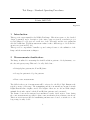
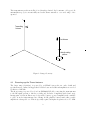
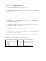
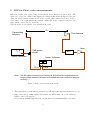
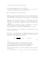
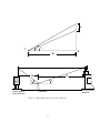
National Centre for Radio Astrophysics
Internal Technical Report
GMRT/FEED/2014
Test Range - Standard Operating Procedures
G.Sankar
Email: [email protected]
Revision
Date
Modification/ Change
Ver. 1
2014
Initial Version
1
Test Range - Standard Operating Procedures
G.Sankar, GMRT-TIFR.
Aug.2013
1
Introduction:
This report is a user manual for the NCRA Test Range. This is in sequence to the detailed
design document[1] and a description of the entire- setup as given in a student’s project
report[2].Chapter 2 of[2] gives an overall view of the Test range and the test equipments
associated with that. Typical measurement results for three different types of feeds and frequencies are given in Ch.3 of[2].
This report is a compendium of smaller reports bearing relevance to the utilization of the
Range and the measurement techniques.
2
Measurements-classification:
The Range is utilized for measuring the far-field radiation patterns of feeds/antennas, over
the chosen frequency range.This can be broadly divided into:
• Principal plane patterns,viz., E and H planes.
• Cross-polar patterns & Co-polar patterns.
• Phase centre measurements.
The SOPs for these sets of measurements will be referenced to the Fig.1. Fig.1 illustrates the
typical geometry of the range. The transmitting and the test antenna are mounted at such
heights that their line-of-sights coincide. The heights of these two are 10.5 m. With a simple
azimuth directional rotation both the E and H-plane patterns can be measured.
The distance between the trans.and test antennas is exactly 134.25 metres. Later during
the course measurements,especially for phase centre,an alternate shorter distance was chosen.
This is at 43.632 metres and the transmitting antenna was relocated; a switch-over to the
longer range is easily doable.
1
The trans.antenna as shown in Fig.1, is a linearly-polarized dipole antenna. A log-periodic
antenna(linear pol.) is conventionally used as the trans. antenna to cover wide range of frequencies.
z
Transmitting
Antenna
Test Antenna
Azimuth rotating
platform
x
y
Figure 1: Range Geometry
2.1
Powering-up the Trans.Antenna:
The longer range (134.25m.) is powered by a OF link between the two ends; details and
specifications are outlined in Appendix-C. Cables losses and additional amplifiers are avoided
by this novel OF link.
The shorter range is powered by a low-loss (LMR400) RF cable,connecting the trans.antenna
to the RF signal generator. On the receiving end, modules of amplifiers (wide-band ones),
having gains of 11,20,30 dBs.are used. A portable, battery -powered amplifier is also available
to place it at the trans.antenna base, having 10 dB gain.The battery inside this portable
amplifier is a chargeable one. This is especially required at higher frequencies above 1.5 GHz.
2
Present test equipments at the range can support up to 3 GHz.Source antennas (trans.)- one
working up to 2 GHz and another up to 3 GHz. are also available.
2.2
Test Antenna Platform:
The platform is a rigid structure, mounted on a rotating disc of 800 mm. diameter, powered
by a geared motor. The motor control and encoder display is part of the system. A Grey-scale
absolute encoder of 13 bits resolution, with two angular limits is provided. the platform can
rotate in both directions and the angular speed is controlled by a multi-turn potentiometer.The
encoder’s digital readout is provided on the front panel and it can be tapped for digital data
acquisition.A brief technical data of the hardware is given below:
• Azimuth coverage: -200◦ to 200◦
• Azimuth rotation speed (max.): 6◦ /sec.
• Encoder resolution: 0.014◦
• Encoder Model: ’Lika’ make- AS58 13/6S-6-E, Absolute enc.
• Az.Drive motor: 0.5HP, 3PH.
• Platform Weight : ∼ 300 kg.(without feed/antenna)
3
SOP for Principal plane Radiation Pattern Measurements:
The digital encoder output and the spectrum analyzer output are connected to a NI data
logger (NI USB-6009). This is can accept 8 analog inputs and has 14-bit I/O.The data acquisition is done by a LabVIEW code, whose details are given in Appendix-D.
The Operating Procedures are listed below:
3
3.1
E-plane patterns:
1. Trans.antenna: Ref.Fig.1. Orient the antenna, such that the dipole arms are parallel to
x -axis.(parallel to xy plane...)
2. Test antenna: Orient the same way like the trans.antenna; the testing channel/dipole
arm should be parallel to x -axis.
Normally a crossed-dipole/dual-orthogonal channel feed arrangement will be mounted.
While one channel/port is aligned, the other channel should be terminated in a 50 Ω
load.
Face the test antenna towards the trans.antenna on line-of-sight.azimuth: 0◦ .
3. Power-up the signal generator & the OF-link. Do not exceed the signal power beyond
+8.0 dBm. Higher power RFs can damage the OF system components.
Choose the correct frequency range.
Note: The Agilent Sig.Gen. : N9301A- make sure that the MOD on/off button is kept
on off-mode, everytime.
4. HP 8108A Spectrum analyzer is used as the power detector. Choose a convenient frequency range, commensurate with Sig.Gen.’s freq.range.Set the default settings of RBW
of 300 kHz and VBW of 3 kHz.
5. Many filters, notch /band-pass types are available at the range; they are identical pieces
of the corresponding frequency band of GMRT front-end electronics.Use the correct ones
based one the frequency-band; a list of available filters is given in Appendix-B.
If any RFI lines are seen closer to the chosen frequency of the Sig.Gen., move away from
that and choose a different frequency.
6. The received signal power should be 30 to 40 dB above noise floor;choose a combination
of the modular amplifiers to realize this.
Check the received power when the test antenna is facing away from the trans.antenna
(azimuth: 180◦ .); here if the power is a few dB above noise floor,it should be okay for
continuing the measurements.
Suitable adapters,couplers are available at Range; a multi-output power supply is also
available to power these amplifiers. Always check the dc voltage at the amp. power ports
with a DMM.
7. When all the above conditions are met, with a slow-speed set on the rotating platform
(few deg./sec.), start the data acquisition from the laptop (LabVIEW code).
4
8. Stop the rotation and data acquiring once a complete 360 deg. rotation is done.
9. The acquired data will be a 2-column vector, containing the encoder output voltage
and the marker power of the Spectrum analyzer. Re-converting them to angles (a liner
calibration curve for the encoder is stored in the laptop; a linear fit eqn. is used to
compute the angles from the dc output voltage).
10. use any graphics software to plot the measured power against the angle-of- rotation; this
is the E-plane pattern of the feed under test.
11. Repeat steps 1 thro 9 for another frequency set in the Sig.Gen.; choose intervals of tens
of MHz for the frequencies,spanning the band of interest.
5
3.2
H-plane patterns:
1. Orient the trans.antenna such that the dipole arms are parallel to y -axis. (parallel to
the yz plane ...)
2. Orient the test antenna - the polarization channel being tested (horizontal / vertical)parallel to y -axis.
Note: Most of the dipole+reflector types of feeds, orient only the dipoles; the reflector
wont be required to re-orient; in the case of aperture-type of feeds(horns, waveguides
etc.) the whole feed should be re-oriented.
Make sure that the orthogonal polarization channel is terminated in 50 Ω load.
3. Follow steps 3 to 7 of the above procedure for E-plane, to get the H-plane pattern.
4. Repeat steps 1 & 2 for another frequency set at the Sig.Gen.
6
4
SOP for Co-polar patterns:
1. Orient the trans.antenna, inclined 45◦ in the xz -plane.
2. Place the test antenna too inclined by 45◦ in the xz -plane.
3. Ensure the orthogonal polarization port is terminated by 50 Ω load.
4. A complete 360◦ azimuth rotation yields the co-planar pattern.
Follow steps 3 to 7 given in Sec.3.
Note: For circularly-symmetric radiation patterns this is average of E & H-planes
patterns.[3]
5. Repeat steps 1 to 4 for another frequency set in the Sig.Gen.
7
5
SOP for Cross-polar patterns:
1. Place the trans.antenna, inclined 45◦ in the xz -plane.
2. Orient the test antenna, inclined 135◦ in the xz -plane,i.e orthogonal to the trans.antenna’s
E-vector plane.
3. The orthogonal polarization port of the test antenna must be terminated by a 50 Ω load.
4. If a co-polar pattern has been measured earlier,the following step can be skipped. Otherwise,repeat step 2 of Sec.4 (i.e.orient the test antenna,inclined by 45◦ to the xz -plane.)
5. Repeat steps 3 to 7 of Sec.3. Azimuth rotation of -70◦ to +70 Ω will be sufficient to
get the cross-polar pattern.
6. The cross-polar pattern’s power level should be scaled down with respect to the co-polar
maximum (i.e at azimuth 0◦ ) being 0 dB.
7. Repeat steps 1 to 4 for a different frequency value.
8. The NI data logger wont be needed here; manually record the data, preferably in a
spreadsheet software and plot it later.
To summarize,the orientations of the trans. and test antennas are given again in the following
Table.
The angles in the Table are with respect to x -axis in the xz -plane.
Pattern Type
E-plane
H-plane
Co-polar
Cross-polar
Angle of Trans.
antenna
0◦
90◦
45◦
45◦
Angle of Test
antenna
0◦
90◦
45◦
135◦
8
Remarks
Az.scan: -180◦ to 180◦
,,
,,
Az.scan: -70◦ to 70◦
6
SOP for Phase centre measurements:
Elaborate details of the phase centre measurements and techniques are given in[4]. The
method,we adopted is outlined in[2].During the initial measurement attempts by the students, the widely varying results as well as not a stable phase values forced us to locate a
closer range of the trans.antenna.Appendix-A outlines the method employed and here the
range distance was reduced to 43.632 m.
Fig.2 shows the block diagram of the measurement set-up.
Ro
Transmitting
Antenna
Test Antenna
Amp.
3 dB power
divider
BPF
Signal Generator
Vector Voltmeter
Ch.A.
Ch.B.
Note : The RF cables connecting to Channels A & B should be of equal electrical
length (phase measured at either ends should be same, within first decimal
accuracy...)
Figure 2: Phase centre measurement set-up
1. The trans.and the test antennas are mounted as per E-plane pattern measurements(vide.Sec.3).
2. First connect the spectrum analyzer and examine the RFI scenario; choose the relatively
RFI-free band of frequencies.
Note down the azimuth angle when the test antenna receives maximum RF power; make
9
a table of these peak-power for the chosen frequencies.
3. Connect the test antenna output to the Vector Voltmeter.
Note: HP 8508A VVM will depict out-of-range if the input Power is ≤ -25 dB. Choose
a higher power at the Sig.Gen. or add more amplifier modules.
4. Move the test antenna by ∼60◦ away from the peak.
5. Similar to the Cross-polar pattern SOP, the data logger won’t be useful for these measurements.Manually record the data in a spreadsheet form. Record the az.angle and the
phase of the received signal (with respect to the input phase of the Sig.Gen.).
6. Make a quick scan of the az.angles : from −60◦ to 60◦ .If the measured phase is well
within -175◦ to 175◦ , it is worth recording. If not, one will see phase-reversal occurring within the scan which would be detrimental to the phase-centre measurements and
computation.
Change the frequency of the Sig.Gen. by a few to tens of MHz. and do another scan;
the new frequency should be free from RFI. Check-up with Step-2.
If problem persists, add a coupler/cable to the trans.antenna side and scan again.
7. Rotate the test antenna by 5 to 10
sian profile of the phase values.
◦
intervals and record the data.One will see a Gaus-
8. From these set of data and knowing the line-of-sight distance, the phase centre at the
chosen frequency of measurement can be calculated.If p is the phase-centre distance
from the axis of rotation(azimuth), then it is given by:
2p· 1 +
(R0 + x0 )
(1 − cos φ)
δ
= δ + 2(R0 + x0 )
(1)
where,
δ is the measured phase difference between the peak and chosen value.
R0 is the line-of-sight diatance between the trans. and test antennas.
x0 is the distance between the rotation axis and the vertical plane of the
test antenna sighting, during the theodolite survey(see Appendix-A).
and
φ is the azimuth angular difference between the peak phase value and the chosen value;
in other words,
φ2 − φ1 corresponding to δ2 − δ1 , where φ1 and δ1 are the values of measured phase
10
and measured az.angle respectively for the peak of the phase-pattern.
9. Repeat the measurements so that a consistent value of the phase-centre location is arrived.
10. Change the frequency and repeat from steps 1 thro’8.
References
[1] G.Sankar,The NCRA Test Range for Wide-band Feeds Development( under
XI Plan),Int.Tech.Report:AG-01/10,Sep.2010.
[2] Vivek.D,Devendra.S,Radiation Pattern characterization of GMRT Feeds, Dept.of
Avionics,IIST,Thiruvananthapuram,April,2012.
[3] Per-simon Kildal,Foundations of Antennas,A Unified Approach, Studentlitteratur
AB,Lund,Swedan,2000.
[4] IEEE Std.149-1979,IEEE Standard Test Procedures for Antennas,John Wiley &
Sons.Inc.,1979.
⋆⋆⋆⋆⋆⋆
11
Appendix - A
A
New location of the Transmitting antenna - for phase centre
measurements
A.1
Introduction:
The need to relocate the transmitting antenna, especially for phase center measurements was
poitned out in the main report. This appendix illustrates the steps taken and records the
theodolite survey procedures and associated computations.
The most viable locations were examined and any such location on the NCRA main building’s terrace would be most suitable, since powering up the trans.antenna would be easier;
the FO technique, as discussed on the main report would be dispensed with, thus reducing
the hardware.
A pole mounted above the water-tank on the northern segment of the building was the
final choice; Fig.1 illustrates the plan view of the locations of trans.and test antenna.
A.2
Survey techniques:
An accurate measurement of the line-of-sight distance between the trans.antenna and the test
antenna platform must be done first. This quantity will be used in the phase-centre measurements. The secondary requirement will be to exactly mark the trans.anteena height on the
pole such that its lies on the horizontal plane of the test antenna’s mounting; in other words,
the centres of both the antennas must coincide on the horizontal,line-of-sight.
A.2.1
Step 1:
A convenient point on the terrace of NCRA building was chosen first, (designated as ’T’ in
Fig.1) as the theodolite station point from where clear visibility of both the trans. ans test
antennas is ensured. The theodolite is positioned exactly over this point(a punch mark is
placed) and the test antenna is viewed.
With azimuth rotation locked on the theodolite, the elevation angles of the bottom and top
1
Water tank
Theodolite
Station " T "
Trans.antenna.
N
"B "
B
R2
T
ψ
R0
R1
NCRA Building
A
"A "
Test Antenna Platform
(on the terrace of R.No.301)
Figure 1: Plan view
centre-lines of the square-frame of the feed-mounting are measured as angles θ1 , θ2 respectively. With the known dimension of the square frame,(k is known; ref. Fig.2) the horizontal
distance R1 is given by:
R1 =
k
tan(θ2 ) − tan(θ1 )
(1)
From the measured values of θ1 , θ2 and k is known, R1 can be computed.
A.2.2
Step 2:
Similarly the horizontal distance R2 can be computed by an exactly similar survey of 2 points
marked on the mounting pole, whose vertical distance,k′ is known. If β1 , β2 are the elevation
angles of the lower and higher points on the mounting pole, then R2 is given by:
R2 =
k′
tan(β2 ) − tan(β1 )
2
(2)
A.2.3
Step 3:
Theodolite being at the same station, next measure the azimuth angle ψ between the
trans.antenna mounting pole and the test antenna platform. As shown in Fig.1, the angle
ψ ,the included angle between R1 andR2 is measured. Hence the line-of-sight distance between the trans. antenna and test antenna, R0 can easily be computed, using the cosine- rule :
R0 =
A.2.4
q
R1 2 + R2 2 − 2R1 R2 cos ψ
(3)
Step 4:
The final step is to mark the line-of-sight on the mounting pole, so that the trans.antenna can
be mounted exactly on the colinear plane to the test antenna’s centre. Refer Fig.2(the lower
half;).
The elevation angle, φ1 of the test antenna’s centre plane is measured. From the figure, it
can be shown that,
R2 tan φ2 = R1 tan φ1
(4)
Angle φ2 can be computed from the above relation, as the remaining quantities are known.
With the computed value for φ2 , that elevation is set and a line is marked on the mounting
pole. This marked-line must coincide with the trans. antenna’s centre-line. Thus the colinearity of both the antennas is achieved.
A.3
Measurements:
Carl-Zeiss electronic theodolite model ELTA-3 was used for the measurement. Following are
the measured parameters and the relevant computed dimensions:
Step 1:
θ2 = 6◦ 11′ 25′′
θ1 = 5◦ 9′ 7′′
and k = 700 mm.
3
k
θ1
T
θ2
A
R1
1111
0000
0000
1111
0000
1111
0000
1111
0000
1111
0000
1111
Water tank &
trans.antenna
R2
φ
R1
φ
2
1
Test antenna
platform
Theodolite
Figure 2: Establishing the horizontal central-line
4
Therefore, R1 = 38.248 metres.
Step 2:
β2 = 8◦ 36′ 10′′
β1 = 7◦ 0′ 23′′
and k′ = 700 mm.
Hence, R2 = 24.658 m.
Step 3:
The measured azimuth angle,ψ = 84◦ 54′ 57′′
So,R0 = 43.632 m.
this is the line-of-sight distance between the trans.and test antennas.This value will be used
for finding the phase centre of any feed being mounted.
Step 4:
The measured elevation angle of the test feed’s centre,
φ1 = 5◦ 36′ 07′′
and therefore,
◦ 36′ 7′′ )
φ2 = arctan 38.248tan(5
24.658
and that works out to be,
φ2 = 8◦ 38′ 54′′
.
This elevation angle is set and a punch mark was done on the mounting pole.
⋆⋆⋆⋆⋆⋆
5
Appendix - B
B
B.1
List of Filters & Amplifiers @Range:
Filters:
Sl.No.
1
2
3
4
5
B.2
Description
327 MHz. BPF
500 MHz. LPF
550-900 MHz.BPF
1600 MHz.LPF
Mobile Notch Filter(925-950 MHz.)
Nos.
1
1
1
1
1
Remarks
Dual-port,cascade-able
Amplifiers:
Sl.No.
1
2
3
4
Device
MAV-11
HMC 740
Serenza
Portable Amp.- Serenza
Nos.
1
1
2
1
Gain
11 dB
30 dB
20 dB
20 dB
⋆⋆⋆⋆⋆⋆
6
Remarks
+12V. supply
+12V.supply
+5V.supply
+5V.Battery
Data logging system using LabVIEW for Antenna test range
G. Sankar, Sanjeet Rai
Objective:To have automatic data logging at antenna test range at NCRA campus.
Introduction:The GMRT system is getting upgraded to achieve seamless coverage from 30 MHz to
1600 MHz. The feed for the upgrade system is tested in antenna test range. To make RF power
measurement easier, we have developed a program using LabVIEW for RF data logging and
angular position measurement.
Rx
Tx
GPIB Interface
Gain
Block
NI 6008 USB DAQ Card
Signal
Generator
DAQ
CARD
Optical
Transmitter
Encoder Output
Test Feed
Rotating
Platform
fiber optics cable
Support
structure
Optical
Receiver
Fig1: Antenna test range setup
Data Acquisition System:LabVIEW is a graphical programming language, from National Instruments. Its GUI
based programming is very user friendly, it can be used for data acquisition, signal processing
and for controlling system.
Component used for data logging system at Antenna test range.
a)
b)
c)
d)
GPIB Card
NI 6008 USB DAQ Card
HP 8590L spectrum analyzer
Computer
Every feed is designed to operate in particular range of frequencies. During the feed test
time, we transmit a continuous wave signal at single frequency, which lie in the respective band
of the feed using a transmitting antenna placed at far distance from the feed (acts as a receiving
antenna). Feed is mounted on a rotating platform which is having encoder; it will give voltage
output according to azimuth angular position of the feed. The output of the encoder is given to
the USB based DAQ card which will continuously acquired angular data in terms of voltage.
GPIB card has been used to acquire RF data from the spectrum analyzer; HP 8590L spectrum
analyzer is having maximum 401 sweep points. It means that whatever is the span of spectrum
analyzer we set using LabVIEW program, it will divide the frequency span by 400 and save the
corresponding power at above sample points. Suppose if we define the frequency range from
200 MHz to 600 MHz i.e. span is 400 MHz, the processing unit within the spectrum analyzer will
divide this 400 MHz span by 400 hence we will get 1 MHz. This means that the RF power at 200
MHz, 201MHZ, and 202 MHz etc up to 600 MHz will get logged during every acquisition cycle.
During testing time we do E and H plane measurement. The feed placed on rotating platform
will scan the transmitting antenna in azimuth plane to get E and H plane data. During scanning,
our program will continuously record the RF power received by the feed and encoder voltage.
The setting for the spectrum analyzer are RBW=300 KHz, VBW=3 KHz and Sweep time= 500ms.
Below is the LabVIEW code that we have used for data logging.
Fig2: Spectrum data logging code control panel.
Fig3: Spectrum data logging code front panel.
In the above LabVIEW code we define the spectrum analyzer visa address, resolution bandwidth
video bandwidth, sweep time, start and stop frequency, acquisition delay time etc.