Download Data-Intensive Linguistics - Department of Linguistics

Data-Intensive Linguistics
Chris Brew and Marc Moens
HCRC Language Technology Group
The University of Edinburgh
April 22, 2004
ii
Contents
I
What is Data-Intensive Linguistics?
1 Introduction
1
3
1.1
Aims of the book . . . . . . . . . . . . . . . . . . . . . . . . .
3
1.2
Recommended reading . . . . . . . . . . . . . . . . . . . . . .
3
1.3
Prerequisites . . . . . . . . . . . . . . . . . . . . . . . . . . .
4
1.4
Chapters . . . . . . . . . . . . . . . . . . . . . . . . . . . . . .
4
1.5
The heart of our approach . . . . . . . . . . . . . . . . . . . .
5
1.6
A first language model . . . . . . . . . . . . . . . . . . . . . .
5
1.7
Ambiguity for beginners . . . . . . . . . . . . . . . . . . . . .
6
1.8
Summary . . . . . . . . . . . . . . . . . . . . . . . . . . . . .
8
1.9
Exercises
8
. . . . . . . . . . . . . . . . . . . . . . . . . . . . .
2 Historical roots of Data-Intensive Linguistics
9
2.1
Why provide a history? . . . . . . . . . . . . . . . . . . . . .
9
2.2
The history . . . . . . . . . . . . . . . . . . . . . . . . . . . .
9
2.3
Motivations for the scientfic study of communication . . . . .
13
2.4
Summary . . . . . . . . . . . . . . . . . . . . . . . . . . . . .
14
2.4.1
Key ideas . . . . . . . . . . . . . . . . . . . . . . . . .
14
2.4.2
Key applications . . . . . . . . . . . . . . . . . . . . .
14
Questions . . . . . . . . . . . . . . . . . . . . . . . . . . . . .
15
2.5
iii
iv
CONTENTS
II
Finding Information in Text
17
3 Tools for finding and displaying text
19
3.0.1
Search tools for data-intensive linguistics
. . . . . . .
20
3.0.2
Using the unix tools . . . . . . . . . . . . . . . . . . .
24
3.1
Sorting and counting text tokens . . . . . . . . . . . . . . . .
24
3.2
Lemmatization . . . . . . . . . . . . . . . . . . . . . . . . . .
30
3.3
Making n-grams . . . . . . . . . . . . . . . . . . . . . . . . .
33
3.4
Filtering: grep . . . . . . . . . . . . . . . . . . . . . . . . . .
35
3.5
Selecting fields . . . . . . . . . . . . . . . . . . . . . . . . . .
38
3.5.1
AWK commands . . . . . . . . . . . . . . . . . . . . .
38
3.5.2
AWK as a programming language . . . . . . . . . . .
46
3.6
PERL programs . . . . . . . . . . . . . . . . . . . . . . . . .
54
3.7
Summary . . . . . . . . . . . . . . . . . . . . . . . . . . . . .
57
3.8
A final exercise. . . . . . . . . . . . . . . . . . . . . . . . . . .
59
3.9
A compendium of unix tools . . . . . . . . . . . . . . . . . .
59
3.9.1
Text processing . . . . . . . . . . . . . . . . . . . . . .
59
3.9.2
Data analysis . . . . . . . . . . . . . . . . . . . . . . .
60
4 Concordances and Collocations
61
4.1
Concordances . . . . . . . . . . . . . . . . . . . . . . . . . . .
61
4.2
Keyword-in-Context index . . . . . . . . . . . . . . . . . . . .
62
4.3
Collocations . . . . . . . . . . . . . . . . . . . . . . . . . . . .
70
4.4
Stuttgart corpus tools . . . . . . . . . . . . . . . . . . . . . .
70
4.4.1
Getting started . . . . . . . . . . . . . . . . . . . . . .
71
4.4.2
Queries . . . . . . . . . . . . . . . . . . . . . . . . . .
73
4.4.3
Manipulating the results . . . . . . . . . . . . . . . . .
75
4.4.4
Other useful things . . . . . . . . . . . . . . . . . . . .
78
v
CONTENTS
III
Collecting and Annotating Corpora
5 Corpus design
81
83
5.1
Introduction . . . . . . . . . . . . . . . . . . . . . . . . . . . .
83
5.2
Choices in corpus design/collection . . . . . . . . . . . . . . .
84
5.2.1
Reference Corpus or Monitor Corpus? . . . . . . . . .
84
5.2.2
Where to get the data? . . . . . . . . . . . . . . . . .
84
5.2.3
Copyright and legal matters . . . . . . . . . . . . . . .
85
5.2.4
Choosing your own corpus . . . . . . . . . . . . . . . .
86
5.2.5
Size . . . . . . . . . . . . . . . . . . . . . . . . . . . .
86
5.2.6
Generating your own corpus . . . . . . . . . . . . . . .
87
5.2.7
Which annotation scheme? . . . . . . . . . . . . . . .
89
An annotated list of corpora . . . . . . . . . . . . . . . . . . .
91
5.3.1
93
5.3
Speech corpora . . . . . . . . . . . . . . . . . . . . . .
6 SGML for Computational Linguists
95
7 Annotation Tools
97
IV
99
Statistics for Data-Intensive Linguistics
8 Probability and Language Models
8.0.2
101
Events and probabilities . . . . . . . . . . . . . . . . . 101
8.1
Statistical models of language . . . . . . . . . . . . . . . . . . 106
8.2
Case study: Language Identification . . . . . . . . . . . . . . 107
8.2.1
Unique strings . . . . . . . . . . . . . . . . . . . . . . 108
8.2.2
Common words . . . . . . . . . . . . . . . . . . . . . . 108
8.2.3
Markov models . . . . . . . . . . . . . . . . . . . . . . 108
8.2.4
Bayesian Decision Rules . . . . . . . . . . . . . . . . . 109
vi
CONTENTS
8.3
Estimating Model Parameters . . . . . . . . . . . . . . . . . . 111
8.3.1
Results . . . . . . . . . . . . . . . . . . . . . . . . . . 112
8.4
Summary . . . . . . . . . . . . . . . . . . . . . . . . . . . . . 112
8.5
Applying probabilities to Data-Intensive Linguistics . . . . . 113
8.5.1
Contingency Tables
. . . . . . . . . . . . . . . . . . . 113
8.5.2
Text preparation . . . . . . . . . . . . . . . . . . . . . 114
8.5.3
Contingency tables . . . . . . . . . . . . . . . . . . . . 115
8.5.4
Counting words in documents . . . . . . . . . . . . . . 119
8.5.5
Introduction . . . . . . . . . . . . . . . . . . . . . . . 119
8.5.6
Bigram probabilities . . . . . . . . . . . . . . . . . . . 120
8.5.7
χ2 . . . . . . . . . . . . . . . . . . . . . . . . . . . . . 121
8.5.8
Words and documents . . . . . . . . . . . . . . . . . . 122
9 Probability and information
123
9.1
Introduction . . . . . . . . . . . . . . . . . . . . . . . . . . . . 123
9.2
Data-intensive grocery selection . . . . . . . . . . . . . . . . . 123
9.3
Entropy . . . . . . . . . . . . . . . . . . . . . . . . . . . . . . 127
9.4
Cross entropy . . . . . . . . . . . . . . . . . . . . . . . . . . . 127
9.5
Summary and self-check . . . . . . . . . . . . . . . . . . . . . 129
9.6
Questions: . . . . . . . . . . . . . . . . . . . . . . . . . . . . . 131
10 Hidden Markov Models and Part of Speech-Tagging
133
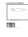
10.1 Graphical presentations of HMMs . . . . . . . . . . . . . . . . 133
10.2 Example . . . . . . . . . . . . . . . . . . . . . . . . . . . . . . 141
10.3 Transcript . . . . . . . . . . . . . . . . . . . . . . . . . . . . . 141
V
Applications of Data-Intensive Linguistics
11 Statistical Parsing
147
149
vii
CONTENTS
11.1 Introduction . . . . . . . . . . . . . . . . . . . . . . . . . . . . 149
11.2 The need for structure . . . . . . . . . . . . . . . . . . . . . . 149
11.3 Why statistical parsing? . . . . . . . . . . . . . . . . . . . . . 153
11.4 The components of a parser . . . . . . . . . . . . . . . . . . . 155
11.5 The standard probabilistic parser . . . . . . . . . . . . . . . . 155
11.6 Varieties of probabilistic parser . . . . . . . . . . . . . . . . . 155
11.6.1 Exhaustive search . . . . . . . . . . . . . . . . . . . . 155
11.6.2 Beam search . . . . . . . . . . . . . . . . . . . . . . . 155
11.6.3 Left incremental parsers . . . . . . . . . . . . . . . . . 155
11.6.4 Alternative figures of merit . . . . . . . . . . . . . . . 155
11.6.5 Lexicalized grammars . . . . . . . . . . . . . . . . . . 156
11.6.6 Parsing as statistical pattern recognition . . . . . . . . 156
11.7 Conventional techniques for shallow parsing . . . . . . . . . . 157
11.8 Summary . . . . . . . . . . . . . . . . . . . . . . . . . . . . . 157
11.9 Exercises
. . . . . . . . . . . . . . . . . . . . . . . . . . . . . 157
Part I
What is Data-Intensive
Linguistics?
1
Chapter 1
Introduction
1.1
Aims of the book
This book has three main aims: familiarity with tools and techniques for
handling text corpora, knowledge of the characteristics of some of the available corpora, and a secure grasp of the fundamentals of statistical natural
language processing. Specific objectives include:
1. grounding in the use of UNIX corpus tools.
2. understanding of probability and information theory as they have been
applied to computational linguistics.
3. knowledge of fundamental techniques of probabilistic language modelling.
4. experience of implementation techniques for corpus tools.
We believe that practical application of the techniques is essential for a clear
understanding of what is going on, so provide exercises which will allow you
to test your understanding and abilities.
1.2
Recommended reading
Charniak (1993) covers statistical language learning from the perspective of
computer science and computational linguistics, and is recommended.
3
4
CHAPTER 1. INTRODUCTION
McEnery and Wilson (1996) is strongly recommended. An electronic version
is available at http://www.ling.lancs.ac.uk/monkey/ihe/linguistics/contents.htm
. This text is less concerned than we are to provide details of the underlying statistical and computational ideas, but is an admirable survey of the
landscape of the field.
One introduction, written for linguists, which comes very close to our approach is Abney (1996). This makes a very clear case for the use of statistical
methods in linguistics. The commentary on Chomsky’s arguments against
Shannon is particularly acute and apposite.
Krenn and Samuelsson (1997) is an ongoing effort to provide a very comprehensive guide to statistics for computational linguists. It should suit
those who want to add a clear and formal grasp of the maths and stats to
a pre-existing background in computational linguistics. It is math-heavy
and application-light, so it is better for people who already know why the
applications to which statistics are being applied are of interest.
? is
1.3
Prerequisites
Prior exposure to some procedural programming language would be desirable. We have tried to make the chapters on corpus search, information
theory, probability and tools as self-contained as possible. It is a fact of life
that this sort of work calls on a wide range of disciplines.
1.4
Chapters
• UNIX Corpus Tools (chapter ??)
• Overview of several selected corpora (chapter 5)
• The IMS Corpus Workbench (chapter 4.4)
• Introduction to probability and contingency tables (chapter 8)
• Information theory. Entropy, Mutual information (chapter 9).
• Hidden Markov Models and text-tagging. Forward-backward algorithm (chapter 10)
1.5. THE HEART OF OUR APPROACH
• Word-sense disambiguation. Clustering techniques (chapter ??)
• Computational Lexicography. (chapter ??)
• Statistical Parsing (chapter ??).
• Information Extraction, MUC, other applications (chapter ??)
• Information Retrieval (chapter ??).
The course provides both awareness of the theoretical issues in statistical
language modelling and practical experience of applying it to corpora. After
completing it, students should be in a position to understand and critique
research papers in statistical computational linguistics. They should also
be aware of the trade-offs involved in selecting statistical techniques for
practical language engineering tasks.
1.5
The heart of our approach
Our approach differs significantly from that of McEnery and Wilson’s textbook, as it does from Charniak’s.
• In general we aim for a decent level of mathematical rigour than the
other sources.
• We introduce some basic probability theory early on.
• We don’t present statistical tests in the usual cookbook style. We feel
that creative data-intensive linguistics demands a flexible approach to
statistics, and we hope that a systematically Bayesian approach will
give students a secure basis from which to apply old principles to new
problems.
1.6
A first language model
Here is an idea of what we mean by the term probabilistic language model.
This is one of the core concepts of Data-Intensive Lingistics.
Imagine a cup of word confetti made by cutting up a copy of “A Case of
Identity” (or sherlock_words). Now imagine picking words out of the cup,
one at a time. On each occasion, you note the word and put it back.
5
6
CHAPTER 1. INTRODUCTION
Given that there are 7070 words in the cup, and 7 of them are sherlock, the
probability of picking sherlock out of the cup is p(sherlock) = 7/7070 =
0.00099. This is the fraction of time you expect to see sherlock if you draw
one word. Similarly, p(holmes) = 46/7070 = 0.0065.
If you are not already comfortable with the ideas of probability and randomness, rest assured that we go into these matters in much more depth
later in the book.
1.7
Ambiguity for beginners
Ambiguity happens when sentences or smaller fragments of text are susceptible of interpretation in more than one way. Computer languages are
typically designed so as to avoid ambiguity, but human languages seem to
be riddled with situations where the listener has to choose between multiple
interpretations. In these cases we say that the listener resolves the ambiguity. For human beings the process of resolution is often unconscious, to
the point that it is sometimes difficult even to recognise that there ever was
any ambiguity. For psychologists ambiguity is an enormously useful tool for
probing the behaviour of the human language faculty, while for computational linguists it is usually an unwelcome problem which must be dealt with
by fair means or foul.
There are several ways in ambiguity can arise:
Lexical ambiguity
Syntactic Semantic
Structural ambiguity
Syntactic . . . Semantic . . .
Pragmatic ambiguity
Pragmatic . . .
7
1.7. AMBIGUITY FOR BEGINNERS
s_maj
s
fpunc
np
vp
noun
verb
Salespeople
sold
np
det
noun
noun
the
dog
biscuits
.
s_maj
s
fpunc
np
vp
noun
verb
Salespeople
sold
np
np
det
noun
noun
the
dog
biscuits
.
s_maj
s
np
fpunc
vp
noun
verb
np
np
Salespeople
sold
np
det
noun
noun
the
dog
biscuits
.
Figure 1.1: Three sentences built on the same words
8
CHAPTER 1. INTRODUCTION
1.8
Summary
1.9
Exercises
Chapter 2
Historical roots of
Data-Intensive Linguistics
This chapter provides a rapid tour of the history of Linguistics and DataIntensive Linguistics1 .
2.1
Why provide a history?
We provide the history not only for its own sake, but as a hook off which to
hang ideas which are crucial in the rest of the course.
2.2
The history
Earliest times The first thing that has to happen in order for linguistics
to be a remotely plausible enterprise is that language must be available in
permanent form. By about 3000 B.C. this had happened for Egyptian hieroglyphics, as well as other written languages. In most cases the texts were
incidental by-products of commerce and trade. Reliable recordings of music
and speech had to wait until the late 19th century, or mid-twentieth century
if high-quality reproduction is required. Data availability is a prerequisite
for many forms of scientific endeavour: For example:
1
The inspiration for this section is a wonderful chapter in McEnery and Wilson which
goes into much more detail than we do. Either the paper version or the WWW version at
[find the address] is well worth reading.
9
10CHAPTER 2. HISTORICAL ROOTS OF DATA-INTENSIVE LINGUISTICS
• Indonesia has undoubtedly had a rich story-telling tradition, but the
climate makes it highly improbable that paper documents will survive
for very long. This limits the potential for diachronic literary studies.
• Nobody really knows how Classical Greek or Shakespearean English
was pronounced. While it is possible to make inferences from contemporary descriptions of the language, from the patterns found in poetry, and from the spellings of evidently onomatapoetic words, there
are many areas in which doubt must remain.
• Little can be said about the acoustics and physiology of the Europeantrained castrato voice. There is one early recording of Alessandro
Moreschi, recorded less than one hour of singing, on wax cylinders, between 1902 and 1904, recorded when he was well past his prime. While
this may be of some interest, one sample is no basis on which to draw
any but the most cautious inferences about such singers. For the film
“Farinelli” (http://www.ircam.fr/produits/technologies/multimedia/farinellie.html) Gérard Corbiau called in IRCAM’s help and did it anyway
Early music specialists constantly face the problem of making intelligent inferences from many different grossly incommensurable sources,
and must learn to live with the inevitable uncertainty. This problem of exploiting limited partial information arises again and again in
data-intensive linguistics.
By around 1000 B.C there was a substantial body of authoritative texts
which we now recognise as the Hebrew Bible. Note that this body of text
is a more or less closed collection of texts imbued with particular authority,
and that major social engineering would be necessary to add or subtract
anything. Texts which are like this are usually termed “canonical”. This is in
marked contrast to a public library, where the contents are open-ended and
constantly changing. An important question for data-intensive linguisticsis
whether language, seen as the object of study, is more like a canon, more
like a public library, or even more like the sort of chat which you randomly
overhear on a bus.
Panini Somewhere between 700 B.C. and 500 B.C. Panini executed a very
modern-seeming study of the (fascinating) properties of Sanskrit. This is
one of the earliest known contributions to the science of linguistics as we
know it today.
2.2. THE HISTORY
Public availability of text The advent of woodblock printing in China
(c 700 AD) and the widespread use of the printing press in Europe (c 1450
AD) meant that books and texts now became available to a much wider
public. By using technology rather than error-prone human transcription,
authors were able to exert more control over the precise contents of texts.
It was now possible for two readers at different ends of a country to pick up
copies of the same edition, and see exactly the same sequence of words. This
is obviously useful if one wants to be able to do reproducible experiments (as
well as for espionage – you can just send the word numbers from an agreed
edition of some code-book, and those not in on the joke will be unable to
decode the message unless they guess which book is being used)
The Rosetta stone Between 1799 and 1820 the French archaeologist
Champollion was able to use a trilingual inscription found on a stone embedded half way up a mountain in what is now Iraq as a key to the correct
interpretation of Egyptian hieroglyphics. The importance of this work is
that it is an early indication that it is often productive to treat language
interpretation as a kind of puzzle. The more text you have to work with the
easier this is going to be.
Käding conducted a heroic feat of social engineering by organising 5000
Prussian analysts to count letter occurrences in 11 million words of text,
using this as the basis of a treatise on spelling rules. It is worth considering
the logistics of doing this in 1897. It now takes a matter of minutes to
obtain similar data from the large corpora of text which are available to us
Taking a 508,219 word sample of the British National Corpus ? we can use
Unix tools (described later) to get the results in table 2.1 for the frequencies
of letter pairs within words. For comparison, table ?? contains the top
30 pairs in the New Testament (180,404 words) Much of the potential of
data-intensive linguistics arises from the ease with which it is possible to do
this sort of thing. The business is in working out what inferences to draw
from such data. Has anything changed since the New Testament version in
question was written? If so, what was it that changed? Spelling conventions?
Patterns of word usage? Perhaps there are lots of proper names in the New
Testament. What exactly happened to the capital letters when we prepared
the table? Was that what we wanted to happen? All these questions deserve
to be answered. But we won’t answer them now . . .
11
12CHAPTER 2. HISTORICAL ROOTS OF DATA-INTENSIVE LINGUISTICS
59677
49318
38676
34196
29223
28556
25962
23772
23437
23278
th
he
in
er
re
an
ou
on
ha
at
21564
20352
19537
19023
18672
18182
16725
16594
15637
15237
nd
it
en
or
ng
to
ve
es
ar
ll
14681
14492
14394
14346
13784
13110
12761
12722
12481
12265
te
st
is
al
ea
hi
me
se
ed
ti
Table 2.1: Letter-letter pairs in a sample of the British national corpus
32446
26939
13182
12899
10974
10581
9631
9593
8880
8116
th
he
nd
an
in
er
ha
re
hi
at
7438
7332
7306
7255
6812
6424
6257
6161
5918
5665
to
or
ou
en
is
of
es
ed
ve
it
Table 2.2: Letter-letter pairs in the complete New Testament
5656
5348
5269
5173
4995
4973
4730
4725
4644
4606
nt
se
on
ng
al
ea
ll
st
me
ar
2.3. MOTIVATIONS FOR THE SCIENTFIC STUDY OF COMMUNICATION
13
2.3
Motivations for the scientfic study of communication
Telegraphy and Telephony In 1832 Samuel F.B. Morse invented the
electric telegraph, and in 1875 Alexander Graham Bell invented the telephone. Communication now becomes a business, and efficiency translates
more or less directly into money. This is a powerful encouragement to design
good ways of passing messages.
Morse code began as a code-book system, where sequences of long and short
dashes represented not letters, as they do in what we know as Morse code,
but whole words. The code was known to the both ends, but the question
arises: is this an efficient way to pass English text from one place to another.
Maybe not, since egregiously stupid things like using especially long codes
for especially short words will make extra work for the telegraphist.
It rapidly became clear that whole word codes were not ideal, so the move
was made to an alphabetic cipher, which being relatively short, could be
memorised by every clerk. Morse did realise that the code would work
better if common letters had short codes, but did not actually take the
trouble to count letters in a sample of text, preferring to derive his estimate
from a quick glance at the relative proportions of different letters in the
compartments of printer’s type box. In spite of this, we now know that
Morse’s assignment of letters, spaces and punctutation to sequences of dots
and dashes is within about 15the best that can be achieved within the limits
of alphabetic ciphers. The potential gain in efficiency from a different cipher
never came close to outweighing the short-term cost of re-training all the
telegraph clerks.
Information Theory Nyquist (1917) established theoretical limits on
how much information could be passed through a telegraph for a given
power, and Nyquist (1928) fixed similar limits on the frequency band needed
to transmit a given amount of information. Also in 1928 Hartley hit upon
a profoundly influential idea: namely that it is in principle possible for any
sequence of symbols to be generated either by a sender acting deliberately
or as the chance outcome of a sequence of random events. He defined the
information content of a message as the logarithm of the number of messages
which might have occurred. We will see later in much more detail how and
why logarithms get into this story. The key idea for the moment is that it is
useful to think of signals as arising from random activities, and to quantify
14CHAPTER 2. HISTORICAL ROOTS OF DATA-INTENSIVE LINGUISTICS
the likelihood that the observed signal arose from the stated model.
2.4
Summary
2.4.1
Key ideas
The following are the key ideas of this chapter.
• Apart from anything else that they may be texts are a publicly available resource for doing science about language. Especially true of
electronic text.
• There are good mathematical tools for studying codes and cyphers,
and some of these are useful in linguistics.
• Linguistics could be seen as a branch of telecommunications engineering, if you wanted to.
• Linguists have to decide whether and how to exploit the availability
of electronic textual resources.
• Actually having the data can be a challenge to the cherished preconceptions of current linguistics. Arguably this is no more than an
artefact of the very recent history of linguistics.
• Statistics is a general method for handling finite samples of potentially infinite (or at least unmanageably large) datasets. It applies
directly to data-intensive linguistics, addressing the central question
of whether the finite samples available to us are in any appropriate
sense representative of the language as a whole. All our arguments
from data to general principles of language and language behaviour
hinge on the assumptions which we make about this crucial issue.
2.4.2
Key applications
The data-intensive approach seems applicable to at least the following
• Explicit models of language acquisition.
• Providing raw materials for psycholinguistic simulations of language
behaviour.
2.5. QUESTIONS
• Focussing the efforts of linguists on topics, such as compound nouns,
which matter more in real life than in current linguistic theory
• Retrieving information.
• Classifying and organising texts and text collections.
• Authorship attribution and forensic linguistics.
• Guiding the choices made by systems which generate text that is supposed to be easy to understand.
• Speech recognition and adaptive user interfaces
• Authoring aids and translation aids
• Cryptography and computer security
It is clear that that the last three applications are the ones with the most
immediate commercial potential, and that the significance of cryptographic
work in affecting our history has already been very great
2.5
Questions
You may not feel in a position to answer these questions. However, I doubt
if anyone is actually able to answer them definitively, so you should attempt
them anyway.
1. Is bird song a language? How about whale songs? Why? Can you
think of ways of supporting your claims using corpus analysis?
2. How would you go about determining authorship of a collection of
disputed text?
3. What is the difference between a language and an artificial code? Why
exactly does Weaver’s idea of treating Russian as a funny encoding of
English seem so strange?
4. A regular seeming signal arrives from a distant star. How would you
try to determine whether this signal is a sample from a language spoken
by some unknown intelligent life form?
15
16CHAPTER 2. HISTORICAL ROOTS OF DATA-INTENSIVE LINGUISTICS
5. A possible objection to the statistical approach is:
“Statistical models can’t be right because they assign a
score even to obvious drivel. This makes them worse than
non-probabilistic grammars, which reject such trash.”
Is this objection reasonable? If so, explain why. If not, explain why
not.
Part II
Finding Information in Text
17
Chapter 3
Tools for finding and
displaying text
This chapter will introduce some basic techniques and operations for use in
data-intensive linguistics. We will show how existing tools (mainly standard
unix tools) and some limited programming can be used to carry out these
operations.
Some of the material on standard unix tools is a revised and extended
version of notes taken at a tutorial given by Ken Church, at Coling 90 in
Helsinki, entitled “Unix for Poets”. We use some of his exercises, adding
variations of our own as appropriate.
One of Church’s examples was the creation of a kwic index, which we
first encountered in chapter 5 of Aho, Kernighan and Weinberger (1988).
In section 4 we discuss this example, provide variations on the program,
including a version in Perl, and compare it with other (more elaborate, but
arguably less flexible) concordance generation tools.
There are more advanced, off-the-shelf tools that can be used for these operations, and several of them will be described later on in these notes. In
theory, these can be used without requiring any programming skills. But
more often than not, available tools will not do quite what you need, and
will need to be adapted. When you do data-intensive linguistics, you will
often spend time experimentally adapting a program written in a language
which you don’t necessarily know all that well. You do need to know the
basics of these programming languages, a text editor, a humility, a positive
attitude, a degree of luck and, if some or all of that is missing, a justified
19
20
CHAPTER 3. TOOLS FOR FINDING AND DISPLAYING TEXT
belief in your ability to find good manuals. The exercises towards the end of
this chapter concentrate on this kind of adaptation of other people’s code.
This chapter therefore has two aims:
1. to introduce some very basic but very useful word operations, like
counting words or finding common neighbours of certain words;
2. to introduce publicly available utilities which can be used to carry out
these operations, or which can be adapted to suit your needs.
The main body of this chapter focuses on particularly important and successful suite of tools — the unix tools. Almost everybody who works with
language data will find themselves using these tools at some point, so it is
worth understanding what is special about these tools and how they differ
from other tools. Before doing this we will take time out to give a more general overview of the tasks to which all the tools are dedicated, since these
are the main tasks of data-intensive linguistics.
3.0.1
Search tools for data-intensive linguistics
The general setup is this: we have a large corpus of (maybe) many millions of
words of text, from which we wish to extract data which bears on a research
question. We might for example, contra Fillmore, be genuinely interested
in the distribution of parts-of-speech in first and second positions of the
sentence. So we need the following
• A way of specifying the sub-parts of the data which are of interest.
We call the language in which such specifications are made a query
language.
• A way of separating the parts of the data which are of interest from
those which merely get in the way. For large corpora it is impractical
to do this by hand. We call the engine which does this a query engine.
Either:
•
a way of displaying the extracted data in a form which the human
user finds easy to scan and assess.
Or: a way of calculating and using some statistical property of the
data which can act as a further filter before anything is displayed
Search tools for data-intensive linguistics
to the user. 1 (We will not discuss appropriate statistical mechanisms in detail for the moment, but the topic will return, in
spades, in later chapters).
We would like a tool which offers a flexible and expressive query language,
a fast and accurate query engine, beautiful and informative displays and
powerful statistical tests. But we can’t always get exactly what we want.
The first design choice we face is that of deciding over which units the query
language operates. It might process text a word at a time, a line at a time, a
sentence at a time, or slurp up whole documents and match queries against
the whole thing. In the unix tools it was decided that most tools should
work either a character at a time or (more commonly) a line at a time. If we
want to work with this convention we will need tools which can re-arrange
text to fit the convention. We might for example want a tool to ensure that
each word occurs on a separate line, or a similar one which does the same
job for sentences. Such tools are usually called filters, and are called to
prepare the data the real business of selecting the text units in which we are
interested. The design strategy of using filters comes into its own when the
corpus format changes: in the absence of filters we might have to change
the main program, but if the main business is sheltered from the messiness
of the real data by a filter we may need to do nothing more than to change
the filter.
The filter and processor architecture can also work when units are marked
out not by line-ends but by some form of bracketing. This style is much
used when the information associated with the text is highly-structured2 .
The Penn Treebank (described in Marcus et al. (1993)) uses this style. The
current extreme of this style uses XML ( a variety of SGML Standard Generalized Markup Language Goldfarb (1990)), essentially an a form of the
bracketing-delimits-unit style of markup, with all sorts of extra facilities for
indicating attributes and relationships which hold of units.
1
Note that the statistical mechanism can operate in either of two modes, in the first
mode it completely removes data which it thinks the human user won’t need to see ,
while in a second, more conservative mode it merely imposes an order on the presentation
of data to the user, so nothing is ever missed, provided only that the user is persistent
enough.
2
For the purposes of this discussion it doesn’t matter much whether the information
has been created by a human being and delivered as a reference corpus, or whether an
earlier tool generates it on the fly from less heavily-annotated text
21
22
CHAPTER 3. TOOLS FOR FINDING AND DISPLAYING TEXT
The next design choice is the query language itself. We could demand that
users fully specify the items which the want, typing in (for example) the
word in which they are interested, but that is of very limited utility, since
you have to know ahead of time exactly what you want. Much better is
to allow a means of specifying (for example) “every sentence containing the
word ’profit”’. Or again “every word containing two or more consecutive
vowels”. There is a tradeoff here, since the more general you make the
query language, the more demanding is the computational task of matching
it against the data.
Performance can often be dramatically improved by indexing the corpus with
information which will speed up the process of query interpretation. The
index of a book is like this, freeing you from the need to read the whole book
in order to find the topic of interest. But of course the indexing strategy can
break down disastrously if the class of queries built into the index fails to
match the class of queries which the user wants to pose. Hence the existence
of reversed-spelling dictionaries and rhyming dictionaries to complement the
usual style. ? is a tool which relies heavily on indexing, but in doing so it
restricts the class of queries which it is able to service. What it can do is
done so fast that is a great tool for interactive exploration by linguists and
lexicographers.
One of the most general solutions to the query-language problem is to allow
users to specify a full-fledged formal grammar for the text fragments in which
they are interested. This gives a great deal of power: and Corley et al. (1997)
has shown that it is possible to achieve adequately efficient implementations
It requires pre-tagged text, but otherwise imposes few constraints on input.
Filters exist for the BNC, for the Penn treebank, and for Susanne. . We
will be working with Gsearch for the first assessed exercise.
See on the Web for more documentation. A sample grammar is in table ??.
Finally, there are toolkits for corpus processing like that described in: McKelvie et al. (1997), which we call LT-NSL or LT-XML, depending (roughly)
on the wind-direction which offer great flexibility and powerful query languages for those who are able and willing to write their own tools. Packaged
in the form of sggrep, the query language is ideally suited for search over
corpora which have been pre-loaded with large amounts of reliable and hierarchically structured annotation. See for further documentation.
It probably isn’t worth going into great detail about ways of displaying
matched data, beyond the comment that visualisation methods are impor-
Search tools for data-intensive linguistics
%
%
%
%
File:
Purpose:
Author:
Date:
23
Grammar
A fairly simple Corset grammar file describing NPs and PPs
Steffan Corley
6th December 1996
#defterm "tag"
% Saves writing
np --> det n1+ pp*
np --> n1+ pp*
np --> np conj np
n1 --> adj* noun+
n1 --> adj* gen_noun n1
n1 --> n1 conj n1
gen_noun --> noun genitive_marker
pp --> prep
%%
% BNC specific part
%%
npdet --> <AT.*>
adj --> <AJ.*>
adj --> <ORD.*>
noun --> <NN.*>
noun --> <NP.*>
genitive_marker --> <POS.*>
prep --> <PR.*>
%
%
%
%
%
%
conj --> <CJ.*>
% Conjunction
% Determiner
Adjective
Ordinal
common noun
proper noun
Saxon genitive
Preposition
ofp --> of np
Table 3.1: a sample Gsearch grammar
24
CHAPTER 3. TOOLS FOR FINDING AND DISPLAYING TEXT
tant if you want human beings to make much sense of what is provided.
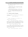
3.0.2
Using the unix tools
So back to the practicalities of the unix tools. . . This chapter is interactive.
To follow this chapter, make sure you have the text files exatext1, exatext2
and exatext3, and code files wc.awk and wc.perl in a directory where you
have write permission. If you don’t have these files, you can take another
plain text file and call it exatext1. You will be told the contents of the
other files in the course of this chapter, so you can create them yourself.
3.1
Sorting and counting text tokens
A tokeniser takes input text and divides it into “tokens”. These are usually
words, although we will see later that the issue of tokenisation is far more
complex than that. In this chapter we will take tokenisation to mean the
identification of words in the text. This is often a useful first step, because
it means one can then count the number of words in a text, or count the
number of different words in a text, or extract all the words that occur
exactly 3 times in a Text, etc.
unix has some facilities which allow you to do this tokenisation. We start
with tr. This “translates” characters. Typical usage is
tr
chars1 chars2 < inputfile > outputfile
which means “copy the characters from the inputfile into the outputfile
and substitute all characters specified in chars1 by chars2”.
For example, tr allows you to change all the characters in the input file into
uppercase characters:
tr ’a-z’ ’A-Z’ < exatext1 | more
This just says “translate every a into A, every b into B, etc.”
Similarly,
tr ’aiou’ e < exatext1 | more
3.1. SORTING AND COUNTING TEXT TOKENS
changes all the vowels in exatext1 into es.
You can also use tr to display all the words in the text on separate lines.
You do this by “translating” everything which isn’t a word (every space or
punctuation mark) into newline (ascii code 012). Of course, if you just
type
tr ’A-Za-z’ ’\012’ < exatext1
each letter in exatext1 is replaced by a newline, and the result (as you can
easily verify) is just a long list of newlines, with only the punctuation marks
remaining.
What we want is exactly the opposite—we are not interested in the punctuation marks, but in everything else. The option -c provides this:
tr -c ’A-Za-z’ ’\012’ < exatext1
Here the complement of letters (i.e. everything which isn’t a letter) is mapped
into a newline. The result now looks as follows:
Text
in
a
class
of
its
own
The
HCRC
Language
Technology
Group
LTG
is
a
technology
transfer
...
25
26
CHAPTER 3. TOOLS FOR FINDING AND DISPLAYING TEXT
There are some white lines in this file. That is because the full stop after a
class of its own is translated into a newline, and the space after the full stop
is also translated into a newline. So after own we have two newlines in the
current output. The option -s ensures that multiple consecutive replacements like this are replaced with just a single occurrence of the replacement
character (in this case: the newline). So with that option, the white lines in
the current output will disappear.
Exercise:
Create a file exa_words with each word in exatext1 on a separate line.
Solution:
Just type tr -cs ’A-Za-z’ ’\012’ < exatext1 > exa_words
You can combine these commands, using unix pipelines (|). For example,
to map all words in the example text in lower case, and then display it one
word per line, you can type:
tr ’A-Z’ ’a-z’ < exatext1 | tr -sc ’a-z’ ’\012’ > exa_tokens
The reason for calling this file exa_tokens will become clear later on. We
will refer back to files created here and in exercises, so it’s useful to follow
these naming conventions.
Another useful unix operation is sort. It sorts lines from the input file,
typically in alphabetical order. Since the output of tr was one word per
line, sort can be used to put these lines in alphabetical order, resulting in
an alphabetical list of all the words in the text. Check the man-page for sort
to find out about other possible options.
Exercise:
Sort all the words in exatext1 in alphabetical order.
Solution:
Just pipeline the tr command with sort: i.e. type
tr -cs ’A-Za-z’ ’\012’ < exatext1 | sort | more
Or to get an alphabetical list of all words in lowercase, you can just type
sort exa_tokens > exa_tokens_alphab.
The file exa_tokens_alphab now contains an alphabetical list of all the word
tokens occurring in exatext1.
3.1. SORTING AND COUNTING TEXT TOKENS
The output so far is an alphabetical list of all words in exatext1, including
duplicates, each on a separate line. You can also produce an alphabetical
list which strips out the duplicates, using sort -u.
Exercise:
Create a file exa_types_alphab, containing each word in exatext1 exactly
once.
Solution:
Just type
sort -u exa_tokens > exa_types_alphab
Sorted lists like this are useful input for a number of other unix tools. For
example, comm can be used to check what two sorted lists have in common.
Have a look at the file stoplist: it contains an alphabetical list of very
common words of the English langage. If you type
comm stoplist exa_types_alphab | more
you will get a 3-column output, displaying in column 1 all the words that
only occur in the file stoplist, in column 2 all words that occur only in
exa_types_alphab, and in column 3 all the words the two files have in
common. Option -1 suppresses column 1, -2 suppresses column 2, etc.
Exercise:
Display all the non-common words in exatext
Solution:
Just type comm -1 -3 stoplist exa_types_alphabetical | more
That compares the two files, but only prints the second column, i.e. those
words which are in exatext but not in the list of common words.
The difference between word types and word tokens should now be clear. A
word token is an occurrence of a word. In exatext1 there are 1,206 word
tokens. You can use the unix command wc (for word count) to find this
out: just type wc -w exatext1.
However, in exatext1 there are only 427 different words or word types.
(Again, you can find this out by doing wc -w exa_types_alphabetical).
There is another tool that can be used to create a list of word types, namely
uniq. This is a unix tool which can be used to remove duplicate adjacent
27
28
CHAPTER 3. TOOLS FOR FINDING AND DISPLAYING TEXT
lines in a file. If we use it to strip duplicate lines out of exa_tokens_alphab
we will be left with an alphabetical list of all wordtypes in exatext1—just
as was achieved by using sort -u. Try it by typing
uniq exa_tokens_alphab | more
The complete chain of commands (or pipe-line) is:
tr -cs ’a-z’ ’\012’ < exa_tokens | sort | uniq | more
Exercise:
Can you check whether the following pipeline will achieve the same
tr -cs ’a-z’ ’\012’ < exa_tokens | uniq | sort | more
Solution:
It won’t: uniq strips out adjacent lines that are identical. To ensure that
identical words end up on adjacent lines, the words have to be put in alphabetical order first. This means that sort has to precede uniq in the
pipeline.
An important option which uniq allows (do check the man-page) is uniq
-c: this still strips out adjacent lines that are identical, but also tells you
how often that line occurred. This means you can use it to turn a sorted
alphabetical list of words and their duplicates into a sorted alphabetical list
of words without duplicates but with their frequency3 Try
uniq -c exa_tokens_alphab > exa_alphab_frequency
The file exa_alphab_frequency contains information like the following:
3
5
35
2
3
1
5
1
3
also
an
and
appear
appears
application
applications
approach
The idea of using a pipeling this way (Under Unix: sort | uniq -c | sort -nr)
to generate numerically sorted frequency lists was published in Bell System Technical
Journal, 57:8, pp 2137-2154.
3.1. SORTING AND COUNTING TEXT TOKENS
29
In other words, there are 3 tokens of the word “also”, 5 tokens of the word
“an”, etc.
Exercise:
Can you see what is odd about the following frequency list?
tr -cs ’A-Za-z’ ’\012’ < exatext1 | sort | uniq -c | more
How would you correct this pipeline?
Solution:
The odd thing is that it counts uppercase and lowercase words separately.
For example, it says there are 11 occurrences of “The” and 74 occurrences
of “the” in exatext1. That is usually not what you want in a frequency list.
If you look in exa_alphab_frequency you will see that that correctly gives
“the” a frequency of occurrence of 85. The complete pipeline to achieve this is
tr ’A-Z’ ’a-z’ < exatext1 | tr -sc ’a-z’ ’\012’ | sort | uniq -c| more
It may be useful to save a version of exatext1 with all words in lower case.
Just type
tr ’A-Z’ ’a-z’ < exatext1 > exatext1_lc
Now that you have a list of all word types in exatext1 and the frequency
with which each word occurs, you can use sort to order the list according
to frequency. The option for numerical ordering is sort -n; and if you add
the option -r it will display the word list in reverse numerical order (i.e. the
most frequent words first).
Exercise:
Generate a frequency list for exatext. Call it exa_freq.
Solution:
One solution is to type
sort -nr < exa_alphab_frequency > exa_freq
The complete pipeline to achieve this was
tr -cs ’a-z’ ’\012’ < exatext1_lc | sort | uniq -c | sort -nr
To recap: first we use tr to map each word onto its own line. Then we sort
the words alphabetically. Next we remove identical adjacent lines using uniq
and use the -c option to mark how often that word occurred in the text.
Finally, we sort that file numerically in reverse order, so that the word
which occurred most often in the text appears at the top of the list.
When you get these long lists of words, it is sometimes useful to use head
or tail to inspect part of the files, or to use the stream editor sed. For
30
CHAPTER 3. TOOLS FOR FINDING AND DISPLAYING TEXT
example, head -12 exa_freq or sed 12q exa_freq will display just the
first 12 lines of exa_freq; tail -5 will display the last 5 lines; tail 14+
will display everything from line 14. sed /indexer/q exa_freq will display
the file exa_freq up to and including the line with the first occurrence of
the item “indexer.
Exercise:
List the top 10 words in exatext1, with their frequency count.
Solution:
Your list should look as follows:
85
42
39
37
35
the
to
of
a
and
34
22
18
15
14
in
text
for
is
this
With the files you already have, the easiest way of doing it is to say
head -10 exa_freq.
The complete pipeline is
tr -cs ’a-z’ ’\012’ < exatext1_lc |sort|uniq -c|sort -nr|head -10
3.2
Lemmatization
The lists of word types we’re producing now still have a kind of redundancy
in them which in many applications you may want to remove. For example,
in exa_alphab_frequency you will find the following:
4
2
1
2
2
12
3
1
at
automatic
base
based
basic
be
been
between
In other words there are 12 occurrences of the word “be”, and 3 of the
word “been”. But clearly “be” and “been” are closely related, and if we are
3.2. LEMMATIZATION
31
interested not in occurrences of words but word types, then we would want
“be” and “been” to be part of the same type.
This can be achieved by means of lemmatisation: it takes all inflectionally
related forms of a word and groups them together under a single lemma.
There are a number of freely available lemmatisers available. This lemmatiser accepts tagged and untagged text, and reduces all nouns and verbs to
their base forms. Use the option -u if the input text is untagged. If you
type morph -u < exatext1 | more the result will look as follows:
the hcrc language technology group (ltg) be a technology transfer
group work in the area of natural language engineering. it work
with client to help them understand and evaluate natural language
process method and to build language engineer solution
If you add the option -s you will see the deriviations explicitly:
the hcrc language technology group (ltg) be+s a technology transfer
group work+ing in the area of natural language engineering. it work+s
with client+s to help them understand and evaluate natural language
process+ing method+s and to build language engineer+ing solution+s
Exercise:
Produce an alphabetical list of the lemmata in exatex1 and their frequencies.
Solution:
If you type
morph -u < exatext1 | tr ’A-Z’ ’a-z’ |
tr -cs ’a-z’ ’\012’ | sort | uniq -c > exa_lemmat_alphab+
the result will be a list containing the following:
4
2
3
2
44
1
at
automatic
base
basic
be
between
Note the difference with the list on page 30: all inflections of “be” have been
reduced to the single lemma “be”.
32
CHAPTER 3. TOOLS FOR FINDING AND DISPLAYING TEXT
Note also that “base” and “based” have been reduced to the lemma “base”,
but “basic” wasn’t reduced to “base”. This lemmatiser only reduces nouns
and verbs to their base form. It doesn’t reduce adjectives to related nouns,
comparatives to base forms, or nominalisations to their verbs. That would
require a far more extensive morphological analysis. However, the adjectives “rule-based” and “statistics-based” were reduced to the nominal lemma
“base”, probaly an “over-lemmatisation”. Similarly, “spelling and and style
checking” is lemmatised as
spell+ing and style checking
which is strictly speaking inconsistent.
It is very difficult to find lemmatisers and morphological analysers that will
do exactly what you want them to do. Developing them from scratch is
extremely time-consuming. Depending on your research project or application, the best option is probably to take an existing one and adapt the source
code to your needs or add some preprocessing or postprocessing tools. For
example, if our source text exatext1 had been tagged, then the lemmatiser
would have known that “rule-based” was an adjective and would not have
reduced it to the lemma “base”.
Wheras for some data-intensive linguistics applications you want to have
more sophisticated lemmatisation and mophological analysis, in other applications less analysis is required. For example, for many information retrieval applications, it is important to know that “technological”, “technologies” and “technology” are related, but there is no real need to know which
English word is the base word of all these words–they can all be grouped
together under the word “technologi”. This kind of reduction of related
words is what stemmers do.
Again, there are a number of stemmers freely available.
If you type stemmer exatext1 | more, the sentence
The HCRC Language Technology Group (LTG) is a technology transfer
group working in the area of natural language engineering.
will come out as
the hcrc languag technologi group ltg i a technologi transfer
group work in the area of natur languag engin
3.3. MAKING N-GRAMS
3.3
Making n-grams
To find out what a word’s most common neighbours are, it is useful to make
a list of bigrams (or trigrams, 4-grams, etc)–i.e. to list every cluster of two
(or three, four, etc) consecutive words in a text.
Using the unix tools introduced in section 3.1 it is possible to create such
n-grams. The starting point is again exa_tokens, the list of all words in the
text, one on each line, all in lowercase. Then we use tail to create the tail
end of that list:
tail +2 exa_tokens > exa_tail2
This creates a list just like exa_tokens except that the first item in the new
list is the second item in the old list. We now paste these two lists together:
paste -d ’ ’ exa_tokens exa_tail2 > exa_bigrams
paste puts files together “horizontally”: the first line in the first file is
pasted to the first line in the second file, etc. (Contrast this with cat which
puts files together “vertically”: it first takes the first file, and then adds to
it the second file.) Each time paste puts two items together it puts a tab
between them. You can change this delimiter to anything else by using the
option -d.
If we use paste on exa_tokens and exa_tail, the n-th word in the first
list will be pasted to the n-th word in the second list, which actually means
that the n-th word in the text is pasted to the n + 1-th word in the text.
With the option -d ’ ’, the separator between the words will be a simple
space. This is the result:
text in
in a
a class
class of
of its
its own
...
Note that the last line in exa_bigrams contains a single word rather than a
bigram.
33
34
CHAPTER 3. TOOLS FOR FINDING AND DISPLAYING TEXT
Exercise:
What are the 5 most frequent trigrams in exatext1.
Solution:
This is the list:
4
4
3
2
2
the human indexer
in the document
categorisation and routing
work on text
we have developed
For creating the trigrams, start again from exa_tokens and exa_tail2 as
before. Then create another file with all words, but starting at the second
word of the original list:
tail +3 exa_tokens > exa_tail3
Finally paste all this together:
paste exa_tokens exa_tail2 exa_tail3 > exa_trigrams
Since all trigrams are on separate lines, you can sort and count them the
same way we did for words:
sort exa_trigrams | uniq -c | sort -nr | head -5
Exercise:
How many 4-grams are there in exatext? How many different ones are there?
(Hint: use wc -l to display a count of lines.)
Solution:
Creating 4-grams should be obvious now:
tail +4 exa_tokens > exa_tail4
paste exa_tokens exa_tail2 exa_tail3 exa_tail4 > exa_fourgrams
A wc -l on exa_fourgrams will reveal that it has 1,213 lines, which means
there are 1,210 4-grams (the last 3 lines in the file are not 4-grams). When
you sort and uniq that file, a wc reveals that there are still 1,200 lines in
the resulting file, i.e. there are 1,197 different 4-grams. Counting and sorting
in the usual way results in the following list:
2
2
2
2
2
underlined in the text
the system displays the
the number of documents
the figure to the
should be assigned to
Of course, there was a simpler way of calculating how many 4-grams there
were: there are 1,213 tokens in exa_tokens, which means that there will be
1,212 bigrams, 1,211 trigrams, 1,210 4-grams, etc.
35
3.4. FILTERING: GREP
3.4
Filtering: grep
When dealing with texts, it is often useful to locate lines that contain a
particular item in a particular place. The unix command grep can be used
for that. Here are some of the options:
grep ’text’
grep ’^text’
grep ’text$’
find all lines containing the word “text”
find all lines beginning with the word “text”
find all lines ending in the word “text”
grep
grep
grep
grep
find
find
find
find
’[0-9]’
’[A-Z]’
’^[A-Z]’
’[a-z]$’
lines
lines
lines
lines
containing any number
containing any uppercase letter
starting with an uppercase
ending with an lowercase
grep ’[aeiouAEIOU]’
grep ’[^aeiouAEIUO]$’
find lines with a vowel
find lines ending with a consonant (i.e. not a vowel)
grep -i ’[aeiou]$’
grep -i ’^[^aeiou]’
find lines ending with a vowel (ignore case)
find lines starting with a consonant (ignore case)
grep -v ’text’
grep -v ’text$’
print all lines except those that contain “text”
print all lines except the ones that end in “text”
The man-page for grep will show you a whole range of other options. Some
examples:
grep -i ’[aeiou].*[aeiou]’ exatext1
find lines with a lowercase vowel, followed by one or more (*) of anything
else (.), followed by another lowercase vowel; i.e. find lines with two or more
vowels.
grep -i ’^[^aeiou]*[aeiou][^aeiou]*$’ exatext1
find lines which have no vowels at the beginning or end, and which have
some vowel in between; i.e. find lines with exactly one vowel (there are none
in exatext1).
grep -i ’[aeiou][aeiou][aeiou]’ exatext1
find lines which contain (words with) sequences of 3 consecutive vowels (it
finds all lines with words like obviously, because of its three consecutive
vowels).
36
CHAPTER 3. TOOLS FOR FINDING AND DISPLAYING TEXT
grep -c displays a count of matching lines rather than displaying the lines
that match. * means “any number of”, i.e. zero or more. In egrep (which
is very similar to grep), you can also use +, which means “one or more”.
Check the man-page for other grep options.
Exercise:
How many words are there in exatext1 that start in uppercase?
Solution:
There are different ways of doing this. However, if you simply do
grep -c ’[A-Z]’ exatext1 then this will only tell you how many lines there
are in exatext1 that contain words with capital letters. To know how many
words there are with capital letters, one should carry out the grep -c operation on a file that only has one word from exatext1 per line:
grep -c ’[A-Z]’ exa_words.
The answer is 79–i.e. there are 79 lines in exa_words with capital letters,
and since there is only one word per line, that means there are 79 words with
capital letters in exatext1.
Exercise:
Can you give a frequency list of the words in exatext1 with two consecutive
vowels?
Solution:
The answer is
5
5
4
4
4
3
...
group
clients
tools
should
noun
our
If we start from a file of lowercase words, one word per line (file exa_tokens
created earlier), then we just grep and sort as follows:
grep ’^[^aeiou]*[aeiou][aeiou][^aeiou]*$’ exa_tokens |
sort | uniq -c | sort -nr
Exercise:
How many words of 5 letters or more are there in exatext1?
Solution:
The answer is 564. Here is one way of calculating this:
grep ’[a-z][a-z][a-z][a-z][a-z]’ exa_tokens | wc -l.
3.4. FILTERING: GREP
37
Exercise:
How many different words of exactly 5 letters are there in exatext1?
Solution:
The answer is 50:
grep ’^[a-z][a-z][a-z][a-z][a-z]$’ exa_tokens | sort | uniq | wc -l.
Exercise:
What is the most frequent 7-letter word in exatext1?
Solution:
The most frequently occurring 7-letter word is “routing”; it occurs 8 times.
You can find this by doing
grep ’^[a-z][a-z][a-z][a-z][a-z][a-z][a-z]$’ exa_tokens
and then piping it through
sort | uniq -c | sort -nr | head -1.
Exercise:
List all words with exactly two non-consecutive vowels.
Solution:
You want to search for words that have 1 vowel, then 1 or more non-vowels,
and then another vowel. The “1 or more non-vowels” can be expressed using
+ in egrep:
egrep ’^[^aeiou]*[aeiou][^aeiou]+[aeiou][^aeiou]*$’ exa_tokens
Exercise:
List all words in exatext1 ending in “-ing”. Which of those words are morphologically derived words? (Hint: spell -v shows morphological derivations.)
Solution:
Let’s start from exa_types_alphab, the alphabetical list of all word types
in exatext1. To find all words ending in “-ing” we need only type
grep ’ing$’ exa_types_alphab.
This includes words like “string”. To see the morphologically derived “-ing”forms, we can use spell -v:
grep ’ing$’ exa_types_alphab | spell -v
which shows the morphological derivations.
38
CHAPTER 3. TOOLS FOR FINDING AND DISPLAYING TEXT
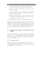
3.5
Selecting fields
3.5.1
AWK commands
Sometimes it is useful to think of the lines in a text as records in a database,
with each word being a “field” in the record. There are tools for extracting
certain fields from database records, which can also be used for extracting
certain words from lines. The most important for these purposes is the awk
programming language. This is a language which can be used to scan lines
in a text to detect certain patterns of text.
For an overview of awk syntax, Aho, Kernighan and Weinberger (1988) is
recommended reading. We briefly describe a few basics of awk syntax, and
provide a full description of two very useful awk applications taken from the
book.
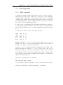
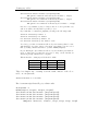
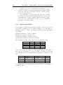
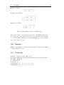
To illustrate the basics of awk, consider first exatext2:
shop
shop
red
work
bowl
noun
verb
adj
noun
noun
41
13
2
17
3
32
7
0
19
1
Imagine that this is a record of some text work you have done. It records
that the word “shop” occurs as a noun 41 times in Text A and 32 times in
Text B, “red” doesn’t occur at all in Text B, etc.
awk can be used to extract information from this kind of file. Each of the
lines in exatext2 is considered to be a record, and each of the records
has 4 fields. Suppose you want to extract all words that occur more than
15 times in Text A. You can do this by asking awk to inspect each line in the
text. Whenever the third field is a number larger than 15, it should print
whatever is in the first field:
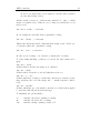
awk ’$3 > 15 {print $1}’ < exatext2
This will return shop and work.
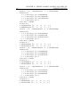
You can ask it to print all nouns that occur more than 10 times in Text A:
awk ’$3 > 10 && $2 == "noun" {print $1}’ < exatext2
AWK commands
39
You can also ask it to find all words that occur more often in Text B (field
4) than in Text A (field 3) (i.e. \$4 > \$3), and to print a message about
the total number of times (i.e. \$3 $4+) that item occurred:
awk ’$4>$3 {print $1,"occurred",$3+$4,"times when used as a",$2 }’ < exatext2
This will return:
work occurred 36 times when used as a noun
So the standard structure of an awk program is
awk pattern {action} < filename
awk scans a sequence of input lines (in this case from the file filename one
after another for lines that match the pattern. For each line that matches
the pattern, awk performs the action. You can specify actions to be carried
out before any input is processed using BEGIN, and actions to be carried out
after the input is completed using END. We will see examples of both of these
later.
To write the patterns you can use $1, $2, ... to find items in field 1,
field 2, etc. If you are looking for an item in any field, you can use $0.
You can ask for values in fields to be greater, smaller, etc than values in
other fields or than an explicitly given bit of information, using operators
like > (more than), < (less than), <= (less than or equal to), >= (more than
or equal to), == (equal to), != (not equal to). Note that you can use == for
strings of letters as well as numbers. You can also do arithmeticic on these
values, using operators like +, -, *, ^ and /.
Also useful are assignment operators. These allow you to assign any kind of
expression to a variable by saying var = expr.
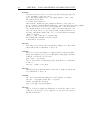
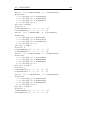
For example, suppose we want to use exatext2 to calculate how often nouns
occur in Text A and how often in Text B. We search field 2 for occurrences
of the string “noun”. Each time we find a match, we take the number of
times it occurs in Text A (the value of field 3) and add that to the value of
some variable texta, and add the value from field 4 (the number of times it
occurred in Text B) to the value of some variable textb:
awk ’$2 == "noun" {texta = texta + $3; textb = textb + $4}
40
CHAPTER 3. TOOLS FOR FINDING AND DISPLAYING TEXT
END {print "Nouns:", texta, "times in Text A and",
textb, "times in Text B"}’ < exatext2
The result you get is:
Nouns: 61 times in Text A and 52 times in Text B
Note that the variables texta and textb are automatically assumed to be 0;
you don’t have to declare them or initialize them. Also note the use of end:
the pattern and instruction are repeated until it doesn’t apply anymore. At
that point, the next instruction (the print instruction) is executed.
You will have noticed the double quotes in patterns like $2 == "noun". The
double quotes mean that field 2 should be identical to the string “noun”.
You can also put a variable there, in which case you don’t use the double
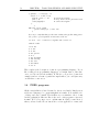
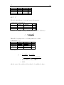
quotes. Consider exatext3 which just contains the following:
a
a
b
c
c
c
d
d
Exercise:
Can you see what the following will achieve?
awk ’$1 != prev { print ; prev = $1}’ < exatext3
Solution:
awk is doing the following: it looks in the first field for something which is
not like prev. At first, prev is not set to anything. So the very first item (a)
satisfies this condition; awk prints it, and sets prev to be a. Then it finds
the next item in the file, which is again a. This time the condition is not
satisfied (since a does now equal the current value of prev) and awk does not
do anything. The next item is b This is different from the current value of
prev So b is printed, and the value of prev is reset to b And so on. The
result is the following:
a
b
c
d
AWK commands
In other words, awk has taken out the duplicates. The little awk program has
the same functionality as uniq.
Another useful operator is ~ which means “matched by” (and !~ which
means “not matched by”). When we were looking for nouns in the second
field we said:
awk ’$2 == "noun"’ < exatext2
In our example file exatext2, that is equivalent to saying
awk ’$2 ~ /noun/ ’ < exatext2
This means: find items in field 2 that match the string “noun”. In the case
of exatext2, this is also equivalent to saying:
awk ’$2 ~ /ou/ ’ < exatext2
In other words, by using ~ you only have to match part of a string.
To define string matching operations you can use the same syntax as for
grep:
awk ’$0 !~ /nou/’
all lines which don’t have the string “nou” anywhere.
awk ’$2 ~ /un$/’
all lines with words in the second field ($2) that end in -un.
awk ’$0 ~ /^...$/’
all lines which have a string of exactly three characters (^ indicates beginning, $ indicates the end of the string, and ... matches any three characters).
awk ’$2 ~ /no|ad/’
all lines which have no or ad anywhere in their second field (when applied
to exatext2, this will pick up noun and adj).
To summarise the options further:
^Z
Z$
^Z$
matches a Z at the beginning of a string
matches a Z at the end of a string
matches a string consisting exactly of Z
41
42
CHAPTER 3. TOOLS FOR FINDING AND DISPLAYING TEXT
^..$
matches
\.$
matches
^[ABC] matches
[^ABC] matches
[^a-z]$ matches
^[a-z]$ matches
[the|an]matches
[a-z]* matches
a string consisting exactly of two characters
a period at the end of a string
an A, B or C at the beginning of a string
any character other than A, B or C
any character other than lowercase a to z at the end of a string
any signle lowercase character string
the or an
strings consisting of zero or more lowercase characters
To produce the output we have so far only used the print statement. It
is possible to format the output of awk more elaborately using the printf
statement. It has the following form:
printf(format, value$_1$, value$_2$, \ldots, value$_n$)
format is the string you want to print verbatim. But the string can have
variables in them (expressed as % followed by a few characters) which the
value statements instantiate: the first % is instantiated by value1 , the
second % by value2 , etc. The % is followed by a few characters, which
indicate how the variable should be formatted. Here are a few examples:
%d means “format as a decimal integer”—so if the value is 31.5, printf
will print 31;
%s means “print as a string of characters”;
%.4s means “print as a string of characters, 4 characters long”—so if the
value is banana printf will print bana;
%g means “print as a digit with non-significant zeros suppressed”;
%-7d means “print as a decimal character, left-aligned in a field that is
7 characters wide.
For example, on page 39 we gave the following awk-code:
awk ’$2 == "noun" {texta = texta + $3; textb = textb + $4}
END {print "Nouns:", texta, "times in Text A and",
textb, "times in Text B"}’ < exatext2
That can be rewritten using the printf command as follows:
awk ’$2 == "noun" {texta = texta + $3; textb = textb + $4}
END {printf "Nouns: %g times in Text A and %g times in Text B\n",
texta, textb}
Note that printf does not print white lines or line breaks. You have to add
those explicitly by means of the newline command \n.
AWK commands
Let us now return to our text file, exatext1 for some exercises.
Exercise:
List all words from exatext1 whose frequency is exactly 7.
Solution:
This is the list:
7
7
7
7
7
units
s
indexer
by
as
You can get this result by typing
awk ’$1 == 7 {print}’ < exa_freq
Exercise:
Can you see what this pipeline will produce?
rev < exa_types_alphab | paste - exa_types_alphab | awk ’$1 == $2’
(Note that rev does not exist on Solaris, but reverse offers a superset of its
functionality. If you are on Solaris, use alias rev ’reverse -c’ instead in
this exercise.)
Notice how in this pipe-line the result of the first unix-command is inserted in
the second command (the paste command) by means of a hyphen. Without
it, paste would not know in which order to paste the files together.
Solution:
You reverse the list of word types and paste it to the original list of word
types. So the output is something like
a
tuoba
evoba
tcartsba
a
about
above
abstract
Then you check whether there are any lines where the first item is the same
as the second item. If they are, then they are spelled the same way in
reverse—in other words, they are the palindromes in exatext1. Apart from
the one-letter words, the only palindromic words in exatext1 are deed and
did.
Exercise:
Can you find all words in exatext1 whose reverse also occurs in exatext1.
These will be the palindromes from the previous exercise, but if evil and live
both occurred in exatext1, they should be included as well.
43
44
CHAPTER 3. TOOLS FOR FINDING AND DISPLAYING TEXT
Solution:
Start the same way as before: reverse the type list but then just append it
to the original list of types and sort it:
rev < exa_types_alphab | cat - exa_types_alphab | sort > temp
The result looks as follows:
a a about above abstract ...
Whereas in the original exa_types_alphab a would have occurred only once,
it now occurs twice. That means that it must have occurred also in rev exa_types_alphab.
In other words, it is a word whose reverse spelling also occurs in exatext1.
We can find all these words by just looking for words in temp that occur
twice. We can use uniq -c to get a frequency list of temp, and then we can
use awk to find all lines with a value of 2 or over in the first field and print
out the second field:
uniq -c < temp | awk ’$1 >= 2 {print $2}’
The resulting list (excluding one-letter words) is:
a deed did no on saw was.
Exercise:
How many word tokens are there in exatext1 ending in -ies? Try it with
awk as well as with a combination of other tools.
Solution:
There are 6 word tokens ending in -ies: agencies (twice), categories (three
times) and companies (once). You can find this by using grep to find lines
ending in -ies in the file of word tokens:
grep ’ies$’ < exa_tokens
Or you can use awk to check in exa_freq for items in the second field that
end in -ies:
awk ’$2 ~ /ies$/’ < exa_freq
Exercise:
Print all word types that start with str and end in -g. Again, use awk as well
as a combination of other tools.
Solution:
The only word in exatext1 starting in str- and ending in -g is “string”:
awk ’$2 ~ /^str.*g$/ {print $2}’ < exa_freq
Another possibility is to use grep:
grep ’^str.*g$’ exa_types_alphab
Exercise:
Suppose you have a stylistic rule which says one should never have a word
ending in -ing followed by a word ending in -ion. Are there any sequences
like that in exatext1?
AWK commands
45
Solution:
There are such sequences, viz. training provision, solving categorisation, existing production, and training collection. You can find them by creating a file
of the bigrams in exatext1 (we did this before; the file is called exa_bigrams)
and then using awk as follows: awk ’$1~/ing$/ && $2~/ion$/’ < exa_bigrams | more
Exercise:
Map exa_tokens_alphab into a file from which duplicate words are removed
but a count is kept as to how often the words occurred in the original file.
Solution:
The simplest solution is of course uniq -c. But the point is to try and do
this in awk. Let us first try and develop this on the simpler file exatext3.
We want to create an awk program which will take this file and return
2
1
3
2
a
b
c
d
In an earlier exercise (page 40) we have already seen how to take out duplicates using awk:
awk ’$1 != prev { print ; prev = $1}’ < exatext3. Now we just have
to add a counter. Let us assume awk has just seen an a; the counter will be
at 1 and prev will be set to a. We get awk to look at the next line. If it
is the same as the current value of prev, then we add one to the counter n.
So if it sees another a, the counter goes up to 2. awk looks at the next line.
If it is different from prev then we print out n as well as the current value
of prev. We reset the counter to 1. And we reset prev to the item we’re
currently looking at. Suppose the next line is b. That is different from the
current value of prev. So we print out n (i.e. 2) and the current value of
prev (i.e. a). We reset the counter to 1. And the value of prev is reset to b.
And we continue as before.
We can express this as follows:
awk ’$1==prev {n=n+1};
$1 != prev {print n, prev; n = 1; prev = $1}’ < exatext3
If you try this, you will see that you get the following result:
2 a
1 b
3 c
It didn’t print information about the frequency of the ds. That is because it
only printed information about a when it came across a b, and it only printed
46
CHAPTER 3. TOOLS FOR FINDING AND DISPLAYING TEXT
information about b when it came across c. Since d is the last element in the
list, it doesn’t get an instruction to print information about d.
So we have to add that, once all the instructions are carried out, it should
also print the current value of n followed by the current value of prev:
awk ’$1==prev {n=n+1};
$1!=prev {print n, prev; n = 1; prev = $1};
END {print n, prev}’
< exatext3
3.5.2
AWK as a programming language
As you can see in the preceding exercises, the awk commands can easily
become quite long. Instead of typing them to your unix prompt, it is useful
to put them into files and execute them as programs. Indeed, awk is more
than a mere unix tool and should really be seen as a programming language
in its own right. Historically, awk is the result of an effort (in 1977) to
generalize grep and sed, and was supposed to be used for writing very
short programs. That is what we have seen so far, but modern-day awk can
do more than this.
The awk code from the previous exercise (page 46) can be saved in a file as
follows:
#!/bin/nawk -f
# input: text tokens (one per line, alphabetical)
# output: print number of occurrences of each word
$1==prev {n=n+1}; $1!=prev {print n, prev; n = 1; prev = $1}
# combine several awk statements by means of semicolons
END { print n,
# awk statements can be broken after commas
prev }
# comments can also be added at the end of a line
The file starts with a standard first line, whose only purpose is to tell unix
to treat the file as an awk program.
Then there are some further comments (preceded by the hashes); they are
not compulsory, but they will help you (and others) remember what your
awk-script was intended for. You can write any text that you like here,
provided that you prefix each line with #. It is good practice to write enough
comments to make the purpose and intended usage of the program evident,
since even you will probably forget this information faster than you think.
AWK as a programming language
47
Then there is the program proper. Note the differences from the way you
type awk commands at the unix prompt—you don’t include the instructions
in single quotes, and the code can be displayed in a typographical layout
that makes it more readable: blank lines can be added before or after statements, and tabs and other white space can be added around operators, all
to increase the readability of the program. Long statements can be broken
after commas, and comments can be added after each broken line. You can
put several statements on a single line if they are separated by semicolons.
And the opening curly bracket of an action must be on the same line as the
pattern is accompanies. The rest of the action can be spread over several
lines, as befits the readability of the program.
If you save the above file as uniqc.awk and make sure it’s executable, then
the command uniqc.awk exatext3 will print out the desired result.
One of awk’s distinguishing features is that it has been tuned for the creation
of text-processing programs. It can be very concise because it uses defaults
a lot. For example, in general it is true that awk statements consist of a
pattern and an action:
pattern { action }
If however you choose to leave out the action, any lines which are matched
by the pattern will be printed unchanged. In other words, the default action
in awk is { print }. This is because most of the time text processing
programs do want to print out whatever they find. Similarly, if you leave
out the pattern the default pattern will match all input lines. And if you
specify the action as print without specifying an argument, what gets
printed is the whole of the current input line.
For example, try the following:
nawk ’gsub("noun","nominal") {print}’ < exatext2
The gsub function globally substitutes any occurrence of “noun” by “nominal”. The print action does not say explicitly what should be printed, and
so just prints out all the matching lines. And if you leave off the print statement, it will still perform that same print action. nawk ’gsub("noun","nominal")’ < exatext2
gives the following result:
shop
nominal
41
32
48
CHAPTER 3. TOOLS FOR FINDING AND DISPLAYING TEXT
work
bowl
nominal
nominal
17
3
19
1
Or consider:
nawk ’$2=substr($2,1,3) {print}’ < exatext2
substr creates substrings: in the second field it will not print the entire field
but a substring, starting at position 1 and lasting for 3 characters: in other
words, “noun” will be replaced by “nou” and “verb” by “ver”. That is the
meaning of substr($2,1,3). However, the print command does not have
an argument and awk prints by default the entire line where this change has
been carried out, not just the affected field, giving the following result:
shop nou 41 32
shop ver 13 7
red adj 2 0
work nou 17 19
bowl nou 3 1
An important type of statement in the writing of awk code is the forstatement. Its general syntax looks as follows:
for (expression1; expression2; expression3)
statement
And here’s an example:
awk ’{for(i=1; i <= NF; i++) print $i}’ < exatext2
It says: set variable i to 1. Then, if the value of i is less than or equal to
the number of fields in the file (for which awk uses the built-in variable NF),
then print that field and increase i by 1 (instead of writing i=i+1 you can
just write i++). In other words, this program prints all input fields, one per
line.
Exercise:
Can you see which of the unix commands discussed in section 3.1 this awk
code corresponds to?
nawk ’{for(i=1; i <= NF; i++) print $i}’ < exatext1
AWK as a programming language
49
Solution:
The output corresponds to what you get when you do
tr -cs ’A-Za-z’ ’\012’ < exatext1
Finally, it is useful to understand how awk deals with arrays. Like variables,
arrays just come into being simply by being mentioned. For example, the
following code can be used with exatext2 to count how many nouns there
are in Text A:
#!/bin/nawk -f
# example of use of array -- for use with exatext2
/noun/ {freq["noun"] += $3}
END {print "There are", freq["noun"], "words of category noun in Text A"}
The program accumulates the occurrences of nouns in the array freq. Each
time an occurrence of “noun” is found, the value associated with the array
freq is increased by whatever number occurs in the third field ($3). The
END action prints the total value. The output is:
There are 61 words of category noun in Text A
To count all occurrences of all categories in Text A, you can combine this
use of arrays with a for-statement:
#!/bin/nawk -f
# for use with exatext2
{freq[$2] += $3}
END {
for (category in freq)
print \
"There are",
freq[category],
"words of type",
category,
"in Text A"}
The for-statement says that for any category in the array freq (i.e. any
category occurring in the second field) you increase the value for that category by whatever value is found in $3. So when the program looks at the
first line of exatext2, it finds a “noun” in $2; an array named freq(noun)
is created and its value is increased by 41 (the number in $3 for that line.
50
CHAPTER 3. TOOLS FOR FINDING AND DISPLAYING TEXT
Next it finds a “verb” in $2 and creates and array freq(verb) and increases
its value from 0 to 13 (the value of $3 on that line). When it comes across
the fourth line, it finds another “noun” in $2 and increases the value of the
array freq(noun) by 17. When it has looked at all the lines in exatext2 it
prints for each “category” the final value for freq[category]:
There are 61 words of type noun in Text A
There are 2 words of type adj in Text A
There are 13 words of type verb in Text A
Exercise:
To summarise what we have seen so far about awk here is a program which
counts the words in a file. It is also available as wc.awk.
1 #!/bin/nawk -f
2 # wordfreq -- print number of occurrences of each word
3 # input: text
4 # output: print number of occurrences of each word
5 { gsub(/[.,:;!?"(){}]/, "")
6
for(i=1; i <= NF; i++)
7
count[$i]++
8
}
9 END {for (w in count)
10
print count[w],w | "sort -rn"
11
}
The line numbers are not part of the program, and the program will not work
if they are left in, but they make it easier to refer to parts of the program.
See if you can work out how the program works.
Solution:
Here is what the program file has in it:
• The first line tells unix to treat the file as an awk program.
• There are then some comments (lines 2-4) preceded by # which indicate
the purpose of the program.
• There is no BEGIN statement, because there is no need for anything to
happen before any input is processed.
• There is a main body (lines 5-8) which is carried out every time awk
sees an input line. Its purpose is to isolate and count the individual
words in the input file: every time awk sees a line it sets up the fields to
refer to parts of that line, then executes the statements within the curly
braces starting at line 5 and ending on line 8. So these statements will
be executed many times, but each time the fields will refer to a different
line of the input file.
AWK as a programming language
• There is an END statement (lines 9-11), which is executed once after
the input has been exhausted. Its purpose is to print out and sort the
accumulated counts.
The main body of the program (lines 5-8) does the following:
• Globally deletes punctuation (line 5), by using awk’s gsub command to
replace punctuation symbols with the null string.
• Sets up a variable i, which is used as a loop counter in a for-loop.
The for statement causes awk to execute the statements in the body
of the loop (in this case just the count[$i]++ statement on line 7)
until the exit-condition of the loop is satisfied. After each execution of
the loop body, the loop counter is incremented (this is specified by the
i++ statement on line 6). The loop continues until it is no longer true
that i <= NF (awk automatically sets up NF to contain the number of
fields when the input line is read in). Taken together with the repeated
execution caused by the arrival of each input line, the net effect is that
count[$i]++ is executed once for every field of every line in the file.
Putting all this together, the effect is that the program traverses the words
in the file, relying on awk to automatically split them into fields, and adding
1 to the appropriate count every time it sees a word.
Once the input has been exhausted, counts contains a count of word-tokens
for every word-type found in the input file. This is what we wanted, but it
remains to output the data in a suitable format.
The simplified version of the output code is:
END {for (w in count)
print count[w],w
}
This is another for loop: this time one which successively sets the the variable
w to all the keys in the count array. For each of these keys we print first the
count count[w] then the key itself w.
The final refinement is to specify that the output should be fed to the unix
sort command before the user sees it. This is done by using a special version
of the print command which is reminiscent of the pipelines you have seen
before.
END {for (w in count)
print count[w],w | "sort -rn"
}
Doing wc.awk exatext1 gives the following result:
51
52
CHAPTER 3. TOOLS FOR FINDING AND DISPLAYING TEXT
74 the
42 to
39 of
...
12 be
11 on
11 The
10 document
It is not quite like what you find in exa_freq because in exa_freq we didn’t
distinguis uppercase and lowercase versions of the same word. You can get
exactly the same result as in exa_freq by doing
tr ’A-Z’ ’a-z’ < exatext1 | wc.awk
Exercise:
What are the 10 most frequent suffixes in exatext? How often do they occur?
Give three examples of each. (Hint: check the man-page for spell and the
option -v.
Solution:
The solution looks as follows:
58 +s abstracters abstracts appears
16 +ed assigned called collected
11 +ing assigning checking consisting
11 +d associated based combined
10 -e+ing dividing handling incoming
10 +ly actually consequently currently
5 +al conditional departmental empirical
3 -y+ied classified identified varied
3 +re representation representational research
3 +er corner indexer number
A first step towards this solution is to use spell -v on all the words in
exatext1 and to sort them. We’ll store the results in a temporary file:
tr -cs ’a-z’ ’\012’ < exatext1_lc | spell -v | sort > temp
temp contains the following information:
+able
+al
+al
+al
+al
+al
+al+ly
...
allowable
conditional
departmental
empirical
medical
technical
empirically
AWK as a programming language
Now we can write a little awk program that will take the information in temp
and for each type of suffix collects all the occurrences of the suffixes. Let’s
call this awk-file suffix.awk. Doing suffix.awk temp will result in
+able
+al
+al+ly
+d
allowable
conditional departmental empirical medical technical
empirically typically
associated based combined compared compiled derived...
Then we can use awk again to print a maximum of three examples for each
suffix and the total frequency of the suffix’s occurrence. For each line we first
check how many fields there are. If the number of fields (nf) is 7, then we
know that that line consists of a suffix in field one, followed by 6 words that
have that suffix. So the total number of times the suffix occured is nf-1. We
print that number, followed by the suffix (which is in field 1 in temp, followed
by whatever is in fields 2, 3 and 4 (i.e. three examples):
suffix.awk temp | awk ’{print NF-1, $1, $2, $3, $4}’ | more We can
then use sort and head to display the most frequent suffixes. The total
pipeline looks as follows:
suffix.awk temp|awk ’{print NF-1,$1,$2,$3,$4}’|sort -nr|head-10
That just leaves the code for suffix.awk. Here is one possibility:
#!/bin/nawk -f
# takes as input the output of spell -v | sort
# finds a morpheme, displays all examples of it
$1==prev {printf "\t%s", $2}
$1!=prev {prev = $1
printf "\n%s\t%s", $1, $2}
END {printf "\n"}
You should now have reached the point where you can work out what this
awk code is doing for you.
We conclude the section with an exercise on counting bigrams instead of
words. You have done this earlier using paste. It is just as easily done in
awk.
Exercise:
Modify wc.awk to count bigrams instead of words. Hint: maintain a variable–
call it prev–which contains the previous word. Note that in awk you can build
a string with a space and assign it to xy in by saying xy = x " " y.
Solution:
Here is the awk solution. The changed lines are commented.
53
54
CHAPTER 3. TOOLS FOR FINDING AND DISPLAYING TEXT
{ gsub(/[.,:;!?"(){}]/, "")
for(i= 1; i <= NF; i++){
bigram = prev " " $i
#
prev = $i
#
count[bigram]++
#
}
}
END {for (w in count)
print count[w],w | "sort
}
build the bigram
keep track of the previous word
count the bigram
-rn"
It is easy to verify that this gives the same results as the pipeline using paste.
We get the top ten bigrams from exatext1 as follows:
tr ’A-Z’ ’a-z’ < exatext1 | bigrams.awk | head -10
with the result:
12 in the
8 to the
8 of the
6 the system
6 in a
5 the document
5 and routing
4 the text
4 the human
4 set of
This completes the description of awk as a programming language. If you
like reading about programming languages, you might want to take time
out to read about it in the manual. If, like me, you prefer to learn from
examples and are tolerant of partial incomprehension, you could just carry
on with these course notes.
3.6
PERL programs
All the unix facilities we have discussed so far are very handy. But the most
widely used language for corpus manipulation is perl. It is available free
of charge and easy to install. The facilities are very similar to those of awk
but the packaging is different. Here is the word count program re-expressed
in perl. We’re not going to try to explain perl in detail, because most of
what you have learned about awk is more-or-less applicable to perl, and
55
3.6. PERL PROGRAMS
because all the evidence is that the people who need perl find it easy to
pick up. It is also available as wc.perl.
while(<>) {
chop;
#
tr/A-Z/a-z/;
#
tr/.,:;!?"(){}//d;
#
foreach $w (split) { #
$count{$w} ++;
#
}
}
remove trailing newline
normalize upper case to lower case
kill punctuation
foreach loop over words
adjust count
open(OUTPUT,"|sort -nr");
# open OUTPUT
while(($key,$value) = each %count) { # each loop over keys and values
print OUTPUT "$value $key\n";
# pipe results to OUTPUT
}
close(OUTPUT);
# remember to close OUTPUT
As in awk, when you program in perl you don’t have to worry about declaring or initializing variables. For comparison here is the awk version repeated,
with some extra comments.
{ gsub(/[.,:;!?"(){}]/, "")
for(i= 1; i <= NF; i++)
count[$i]++
}
END {for (w in count)
print count[w],w | "sort -rn"
}
# kill punctuation
# for loop over fields
# adjust count
# for loop over keys
# pipe output to sort process
The following are the important differences between wc.awk and wc.perl:
1. perl uses different syntax. Variables are marked with $ and statements finish with a semi-colon. The array brackets are different too.
2. Where awk uses an implicit loop over the lines in the input file perl
uses an explicit while loop. Input lines are read in using <>. Similarly
there is no END statement in perl . Instead the program continues once
the while loop is done.
56
CHAPTER 3. TOOLS FOR FINDING AND DISPLAYING TEXT
3. Where awk has gsub, perl has tr. You can see another use of tr in
the line tr/A-Z/a-z/;. This is analogous to the Unix command tr
which we saw earlier.
4. Where awk implicitly splits the fields of the input lines and sets NF,
the perl program explicitly calls split to break the line into fields.
5. perl uses a foreach loop to iterate over the fields in the split line
(underlyingly foreach involves an array of elements. In fact perl has
several sorts of arrays, and many other facilities not illustrated here).
awk uses a C style for loop to carry out the same iteration.
6. Both programs finish off by outputting all the elements of the count
array to a sort process. Where awk specifies the sort process as a
kind of side-condition to the print statement, perl opens a file handle
to the sort process, explicitly closing it once its usefulness has been
exhausted.
The general trend is that awk programs are more concise than sensibly written perl programs. perl also has a very rich infra-structure of pre-packaged
libraries . Whatever you want to do, it is worth checking that there isn’t
already a freely available perl module for doing it.
awk, by contrast, is orderly and small, offering a very well chosen set of
facilities, but lacking the verdant richness and useful undergrowth of perl.
The definitive awk text by Aho, Weinberger and Kernighan is 210 pages of
lucid technical writing, whereas perl has tens of large books written about
it. We particularly recommend “Learning Perl” by Randal Schwartz. It is
unlikely that you will ever feel constrained by perl, but awk can be limiting
when you don’t want the default behaviour of the input loop. To a great
extent this will come down to a matter of personal choice. We prefer both,
frequently at the same time, but for different reasons.
Exercise:
Modify wc.perl to count bigrams instead of words. You should find that
this is a matter of making the same change as in the awk exercise earlier In
perl you can build a string with a space in and assign it to $xy by saying
$xy = ‘‘$x $y’’;
Solution:
The perl solution is analogous to the awk one:
57
3.7. SUMMARY
while(<>) {
chop;
tr/A-Z/a-z/;
tr/.,:;!?"(){}//d;
foreach $w (split) {
$bigram = "$prev $w";
$prev = $w;
$count{$bigram} ++;
}
}
# make the bigram
# update the previous word
# count the bigram
open(OUTPUT,"|sort -nr");
while(($key,$value) = each %count) {
print OUTPUT "$value $key\n";
}
close(OUTPUT);
You might want to think about how to generalize this program to produce
trigrams, 4-grams and longer sequences.
3.7
Summary
In this chapter we have used some generally available unix tools which assist
in handling large collections of text. We have shown you how to tokenise
text, make lists of bigrams or 3-grams, compile frequency lists, etc.
We have so far given relatively little motivation for why you would want to
do any of these things, concentrating instead on how you can do them. In
the following chapters you will gradually get more of a feel for the usefulness
of these basic techniques.
To conclude, here is a handy cheat sheet which summarises the basic unix
operations discussed in this chapter.
58
CHAPTER 3. TOOLS FOR FINDING AND DISPLAYING TEXT
cut
cut
cut
cut
-f2
-c2,5
-f2-4,6
-f2 -d":"
delete all but
delete all but
delete all but
delete all but
the default)
the second field of each line
the second and fifth character of each line
second, third, fourth and sixth fields of each line
the second field where ”:” is the field delimiter (tab is
grep
grep -v
grep -c
fgrep
egrep
find lines containing a certain pattern
print all lines except those containing the pattern
print only a count of the lines containing the pattern
same as grep but searches for a character string
same as grep, but whereas grep only recognises certain special characters, egrep recognises all regular expressions
head -12
tail -5
tail 14+
output first 12 lines
output last 5 lines
output from line 14
paste
paste -d">"
combine files “horizontally” by appending corresponding lines
like paste, but set the delimiter to > (tab is the default delimiter).
sort
sort -n
sort -r
sort into alphabetical order
sort into numerical order
sort into reverse order (highest first)
tr ’A-Z’ ’a-z’
tr -d ’ab’
tr -s "a" "b"
translate all uppercase letters into lowercase letters
delete all occurrences of a and b
translate all a to b and reduce any string of consecutive b to just one
b.
uniq
uniq -d
uniq -c
remove duplicate lines
output only duplicate lines
remove duplicate lines and count duplicates
wc -c
wc -l
wc -w
count characters
count lines
count words
3.8. A FINAL EXERCISE.
3.8
A final exercise.
The following exercise is hard, and is provided, without explicit solution, as
a challenge to your ingenuity.
Exercise:
Write a program (in awk perl or any other computer language) which reads
two sorted text files and generates a sorted list of the words which are common
to both files. Write a second program which takes the same input, producing
the list of words found only in the first file. What happens if the second file
is an authoritative dictionary and the first is made from a document full of
spelling errors? How is this useful? Describe the sorts of spelling error which
this approach won’t find. Does this matter?
Solution:
An industrial strength solution to this problem is described in chapter 13
of Jon Bentley’s Programming Pearls. It describes the unix tool spell,
which is a spelling checker. It just points out words which might be wrong.
Spelling suggesters, which detect spelling errors, then offer possible replacement strings to the human user, are at the edges of research. Spelling correctors, which don’t feel the need of human intervention, are probably a bad
idea. Automatic detection of hidden spelling errors (the ones where the output is real word, but not the word which the writer intended) is an active
research issue.
3.9
A compendium of unix tools
This section lists some more tools which are available on the Edinburgh
Cognitive Science systems. We are not going to go into these tools in any
detail, but we have found them useful in the past. They are all designed for
use in Unix pipelines with textual input. To use these you should read the
manual pages. Don’t worry if some of the descriptions don’t make sense to
you yet. We plan to add to this list and make it available on-line.
3.9.1
Text processing
The following are provided by Ted Dunning from New Mexico State University. They have some overlap with stuff we have developed so far, but have
extra facilities, and are often faster:
59
60
CHAPTER 3. TOOLS FOR FINDING AND DISPLAYING TEXT
1. hwcount – count tokens, like sort | uniq -c but faster.
2. fwords – a fast version of words for segmenting the English text
3. cgram – convert text into character n-grams
4. grams – no man-page , but cat file | grams 3 prints all bigrams in
file.
5. compare – compare frequencies of strings in two files.
6. chi2 – several measures of how “sticky” words are.
3.9.2
Data analysis
These are from Gary Perlman’s |stat package (pronounced “pipe stat”).
They are excellent, but not 8-bit clean, so should be used cautiously, if it all
with texts that contain accented or other non-ASCII characters.
1. pair – Paired data points analysis and plots
2. desc – Pescribing a single data distribution
3. anova – Analysis of variance.
4. rankrel – Rank tests on related samples
5. rankind – Rank tests on independent samples
6. regress – Regression analysis
7. colex – Extract columns from a file
8. linex – Extract lines from a file
Chapter 4
Concordances and
Collocations
4.1
Concordances
In chapter 3 we described some tools that produce lists with word frequencies
or lists of bigrams for a given text. Inspecting such lists gives you a good
idea as to the overall profile of the text; it may point you to certain words or
bigrams that look unusual and whose behaviour you want to study further.
To do that, you probably want to see those words in their original context.
A word with its context is a concordance. Concordance programs let you
specify a word, a set of words, a part-of-speech tag or possibly some other
kind of keyword and then return a concordance for each occurrence of that
keyword.
Suppose that a preliminary study of words in sherlock has suggested that
the usage of the word “remember” is worth looking into further—e.g. to
check whether it is used transitively as well as intransitively. A good starting
point for such a study is a concordance for “remember”. The typical way of
displaying such a concordance is as follows:
and then afterwards they
d about it. He laughed, I
important. Can you
arate us, I was always to
eave the papers here, and
remembered us, and sent them to moth
remember, and shrugged his shoulders
remember any other little things abo
remember that I was pledged to him,
remember the advice which I have giv
61
62
CHAPTER 4. CONCORDANCES AND COLLOCATIONS
l not believe me. You may remember the Old Persian saying, the
In other words, the keyword (in this case “remember”) appears roughly in
the middle of each line, and each line has some predetermined number of
characters. This way of displaying a concordance is called a Keyword in
Context index, or kwic index.
A kwic index is not the only way of displaying a concordance. You could
display each sentence or paragraph the keyword occurs in, rather than some
words to the left and right of the keyword. But in what follows we will
concentrate on kwic indexes. We will first describe code that allows you to
build kwic indexes. In chapter4.4, we describe a graphical interface which
makes it easy to build certain types of concordances.
4.2
Keyword-in-Context index
This section describes an awk program for presenting a text file in the form
of a kwic index. When applied to exatext1 the result would contain the
following:
considers appropriate for this
and-alone product by technical
agencies who publish technical
s to allow researchers to find
short, to try and
lters to collect messages from
Indexers can also
thout human intervention. News
The ‘Terms’ menu contains
ks on that particular keyword,
by a robust noun-group parser.
In
unit occurs at
abstracts to
abstract. In the top right han
abstract. When the indexer
abstracters on their home
abstracts from a wide collecti
abstracts of publications that
abstracts to allow researchers
achieve full text interpretati
across the world, scan
actually appear in the documen
add new keywords which they th
against descriptor assignments
agencies
agencies who publish technical
all allowable terms for a part
all occurrences of
All the documents in a large
all these applications, the as
all. This gives an estimate of
allow researchers to find abst
4.2. KEYWORD-IN-CONTEXT INDEX
written by clinicians, both to
allow the compilation of perfo
The programming task of making a kwic index is described in great detail
in chapter 5 of Aho, Kernighan and Weinberger (1988). It turns out that
the unix pipeline approach is amazingly well-suited to this task once the
correct decomposition of the problem has been found. The key insight is
that the following three-step decomposition of the problem is good:
• A first program generates rotations of the input line so that each word
in turn is at the front.
• A sort brings together lines starting with the same first word.
• The final program undoes the original rotation, putting the words back
in their original order.
This can be done in awk in two small programs which fit on half a page.
Admittedly the programs pack a lot of awk lore into a small space, but
because they are so short they can be explained in detail.
The rotate program looks as follows (also available as rotate.awk):
1
2
3
4
5
{ print $0
for(i = length($0); i > 0; i--)
if(substr($0,i,1) == " ")
print substr($0,i+1) "\t" substr($0,1,i-1)
}
Again, the line numbers are only there to allow discussion. The first line
prints out each input line in its original order (because $0 refers to the whole
input line). Line 2 is a for loop which counts the variable i down from the
length (in characters) of the input to 1, inclusive. Lines 3 happens for every
value of i. It tests whether the substring of length 1 at position i is a single
blank. If it is, line 4 is executed, which prints out the string formed by
concatenating the following things
• the substring of $0 starting at position i+1 (and carrying on to the
end of the line, because the third argument of substr is optional –
if it is not supplied, awk assumes it is meant to carry copying until
it reaches the end of the line. This is another example of awk being
concise by employing defaults.)
63
64
CHAPTER 4. CONCORDANCES AND COLLOCATIONS
• A single tab character. The presence of this character is crucial to the
overall effect, since the unrotate program relies on its presence.
• The substring from the start of $0 to position i-1.
If the input is exatext1, then the output of the first stage is as follows:
The HCRC Language Technology Group (LTG) is a technology transfer
transfer
The HCRC Language Technology Group (LTG) is a technology
technology transfer
The HCRC Language Technology Group (LTG) is a
a technology transfer
The HCRC Language Technology Group (LTG) is
is a technology transfer
The HCRC Language Technology Group (LTG)
(LTG) is a technology transfer The HCRC Language Technology Group
Group (LTG) is a technology transfer
The HCRC Language Technology
Technology Group (LTG) is a technology transfer The HCRC Language
...
The second stage of the pipeline is just sort -f. The -f option sorts together upper and lower case words (so “This” and “this” are not separated).
The output becomes:
abstract the human indexer is currently working on. The bottom left
abstract. In the top right hand corner, the system displays the
abstract. When the indexer
keywords it considers appropriate for this
abstracters on their home
used as a stand-alone product by technical
abstracts from a wide collection of
agencies who publish technical
abstracts of publications that abstracts to allow researchers to find
abstracts to allow researchers to find abstracts of publications that
achieve full text interpretation.
short, to try and
across the world, scan use message filters to collect messages from
...
The unrotate program is even shorter than the rotate program (available
as unrotate.awk):
1 BEGIN {FS= "\t"; WID = 30}
2
{ printf ("%" WID "s %s\n",
3
substr($2,length($2)-WID+1),substr($1,1,WID))
4
}
4.2. KEYWORD-IN-CONTEXT INDEX
Note the use of the built in variable FS (for Field Separator). FS is given
a single tab character as its value. This means that awk will automatically
split input lines at tabs, rather than (as is the default) any white-space
character. This in turn means that when the main body (lines 2-4) processes
lines, they are split in two at the tab characters which were inserted by the
rotate program1 .
The program uses printf as explained on page 42. Note how it constructs the string that is to be printed (WID) on the fly from the expression
"%" WID "s %s\n".
Putting the three components together, we have:
rotate.awk example | sort -f | unrotate.awk | more
Try this. The result will contain lines like the following:
and-alone product by technical
agencies who publish technical
s to allow researchers to find
short, to try and
lters to collect messages from
Indexers can also
abstracters on their home PCs
abstracts from a wide collecti
abstracts of publications that
abstracts to allow researchers
achieve full text interpretati
across the world, scan
actually appear in the documen
add new keywords which they th
against descriptor assignments
...
Exercise:
Compare the following output of the kwic index software with that above:
and-alone product by technical
agencies who publish technical
s to allow researchers to find
st assigning keywords to these
ge to is too short, to try and
lters to collect messages from
tching --- does a fixed string
Indexers can also
ocument representational units
1
abstracters on their home PCs.
abstracts from a wide collecti
abstracts of publications that
abstracts to allow researchers
achieve full text interpretati
across the world, scan them, a
actually appear in the documen
add new keywords which they th
against descriptor assignments
The input file had better not contain tab characters. You might like to work out what
will happen if this precondition is violated. If push comes to shove you can use unix tools
like tr to remove extraneous tabs
65
66
CHAPTER 4. CONCORDANCES AND COLLOCATIONS
Can you see what may have caused the difference?
Solution:
The kwic index software goes through exatext1 line by line. Because the
word “actually” appears at the start of a line in the exatext1 file, it shows
up in the kwic index with no context to its left. Strictly speaking, that’s
wrong.
You can avoid that problem by removing linebreaks in the input file.
example, you could take out all the linebreaks, still leaving in titles
paragraph breaks. If you then run the kwic software, only the start
paragraph will show up in the kwic index with no context to its left;
the last word of a paragraph will show up with no context to its right.
For
and
of a
and
Exercise:
Redo the kwic index but add a stoplist so that the very common words like
“a” and “the” are not taken as keywords.
Solution:
The best way to do this is to write a program which prints all lines except
those that start with common words. Here’s a list of words you may want to
exclude:
$1 !~ /^(a|A|an|An|and|And|for|For|if|If|in|In|of|Of|the|The|to|To)$/
The !~ means “does not match” so the effect of the program is to reject
all lines which begin with the common words. This can be inserted into the
pipeline after rotate, as follows:
rotate.awk example |stop.awk |
sort -f | unrotate.awk
Aside from their use as a tool for organising data in service of linguistics
kwic indices can also be useful for language engineering tasks, such as catching inconsistent application of spelling and style conventions. The kwic
index to exatext1 contains the lines:
incoming mail and sort it into
classify them into a number of
solving
In our experience of
text
omatic and semi-automatic text
categories is not an arbitrary
categories like
categories so that relevant
categorisation and routing pro
categorisation and routing pro
categorisation and routing sol
categorisation is also an impo
categorisation system, SISTA.
4.2. KEYWORD-IN-CONTEXT INDEX
Our work on text
Text
lications, the assignment of a
the likelihood that a certain
67
categorisation tools are used
categorization and routing are
categorization and routing has
categorization and text routin
category or set of
category should be
This shows that
• The spelling of categori[sz]ation is not consistent through the document. Probably one or the other should be used throughout.
• There are two different formulations of the pattern (Text) categorisation
and (text) routing. It looks as if these usages are free variation
rather than anything intended by the author. Guidelines for technical writing typically discourage this, on the grounds that it might be
confusing. kwic indices can make it much easier to spot the problem.
It is another matter whether it is in fact a good idea to remove the
inconsistency.
Exercise:
Modify the code to produce nicer looking output using ASCII art.
Solution:
We format the words as a table, using features of printf which are not worth
discussing here. One thing which is worth discussing is the use of index to
try to find a trailing space after the first word. If there is a space, we use the
knowledge of the position to split the string into three parts. If we didn’t
find a space, we must be at the end of the line, so we set the variable pos
as if there really were a space after the end of the line. This lets us use the
same code for both cases:
• The prefix
• The word itself
• The postfix
BEGIN {FS= "\t"; WID = 30; WORDLEN=12; line()}
{ pos = index($1," ")
if(!pos) {
pos = length($1)+1;
}
printf ("|%" WID "s | %-" WORDLEN "s| %-" WID "s|\n",
68
CHAPTER 4. CONCORDANCES AND COLLOCATIONS
substr($2,length($2)-WID+1),
substr($1,1,pos-1),
substr($1,pos+1,WID))
}
END { line() }
function line () {print "---...---"}
We also take the opportunity to define a tiny function for drawing lines of
the right length at the beginning and end of the table. Some of the dashes
are omitted in the listing.
Alternative solution:
Another way to write the same program uses a second function to do the
output to the screen, as follows:
BEGIN {FS= "\t"; WID = 30; WORDLEN=12; line()}
{ pos = index($1," ")
if(!pos) { pos = length($1)+1}
cells($2,$1,pos ) }
END { line() }
function cells(prefix,suffix,pos) {
printf ("|%" WID "s | %-" WORDLEN "s| %-" WID "s|\n",
substr(prefix,length(prefix)-WID+1),
substr(suffix,1,pos-1),
substr(suffix,pos+1,WID))
}
function line () {print "---...---"}
This has the merit that it clarifies the purpose of the main program, and
isolates the clunky manoeuvres with printf in a single location. The second
version would be slightly easier to modify if you needed a kwic index program
which output direct to LATEX. This program is available as unrotate3.awk.
Output from unrotate3 is shown in table 4.1
Exercise:
Write the program which generates the LATEX kwic index. (Obviously you
need to know what input LATEX expects, so this question is for LATEXies only.)
Solution:
Only small changes are needed:
BEGIN {FS= "\t"; WID = 30; start_table()}
{ pos = index($1," ")
4.2. KEYWORD-IN-CONTEXT INDEX
69
------------------------------------------------------------------------------| ...
|
|
|
|considers appropriate for this | abstract.
| When the indexer clicks on a k|
|and-alone product by technical | abstracters | on their home PCs. Above, we g|
|agencies who publish technical | abstracts
| from a wide collection of jour|
|s to allow researchers to find | abstracts
| of publications that may be of|
|st assigning keywords to these | abstracts
| to allow researchers to find a|
|ge to is too short, to try and | achieve
| full text interpretation.
|
|lters to collect messages from | across
| the world, scan them, and clas|
|tching --- does a fixed string | actually
| appear in the document? At the|
| ...
|
|
|
------------------------------------------------------------------------------Table 4.1: ASCII output from unrotate3.awk
if(!pos) { pos = length($1)+1}
cells($2,$1,pos ) }
END { end_table() }
function cells(prefix,suffix,pos) {
printf ("%s & %s & %s \\\\ \\hline \n",
substr(prefix,length(prefix)-WID+1),
substr(suffix,1,pos-1),
substr(suffix,pos+1,WID))
}
function start_table () {
print "{\\small"
print "\\begin{tabular}{|r|l|l|} \\hline"
print "\\multicolumn{1}{|l|}{Prefix} &"
print "Word &"
print "\\multicolumn{1}{l|}{Suffix} \\\\ \\hline \\hline"
}
function end_table () {
print "\\end{tabular}"
print "}"
}
The only point of general interest is that you need to write \\ inside strings
in order to get \ in the output. The result can be seen in table 4.2.
70
CHAPTER 4. CONCORDANCES AND COLLOCATIONS
Prefix
considers appropriate for this
and-alone product by technical
agencies who publish technical
s to allow researchers to find
st assigning keywords to these
ge to is too short, to try and
lters to collect messages from
tching — does a fixed string
Word
...
abstract.
abstracters
abstracts
abstracts
abstracts
achieve
across
actually
...
Suffix
When the indexer clicks on a k
on their home PCs. Above, we g
from a wide collection of jour
of publications that may be of
to allow researchers to find a
full text interpretation.
the world, scan them, and clas
appear in the document? At the
Table 4.2: LATEX output from unrotate4.awk
4.3
Collocations
Concordances are a useful tool for inspecting the context particular keywords
appear in. But it is not a very good basis for doing a real quantitative analysis: the number of hits you get may be very high; more importantly, the
results are still unordered. Of course, the concordances can be ordered alphabetically, but to start real quantitative work you to make some decisions
about which occurrences are of the same type. This requires further analysis
of the concordances, and this is where collocation analysis comes in.
Collocation is the occurrence of a number of words within a short space of
each other in a text. For example, you might be interested in the occurrence
of a particular verb with a particular preposition. What you want to do in
particular is examine to which extent this collocation of verb and preposition
is different from the pattern that you would have expected for those words,
and so statistical and other significance measures come in.
But before we turn to these statistical measures, we’ll first describe a tool
for extracting collocations from text.
4.4
Stuttgart corpus tools
The ims Corpus Workbench is an extremely useful tool for data-intensive linguistic applications. It was developed by various people at Stuttgart’s Institut für Maschinelle Sprachverarbeitung. You can find information about the
ims Corpus Workbench on their web page: http://www.ims.uni-stuttgart.de/Tools/CorpusTo
Getting started
71
You will also find information there about how to download the workbench,
and conditions of use.
In Edinburgh, the software has already been downloaded and
installed. To use it, make sure you are logged in to burns and
then set the following environment variables:
burns:
burns:
burns:
burns:
setenv UHOME /usr/local/ims-cwb
set path = ($UHOME/bin $UHOME/uid $path)
setenv CORPUS_REGISTRY $UHOME/registry
setenv MANPATH $UHOME/man:$MANPATH
You can now start the workbench by just typing xkwic to the
unix prompt.
There are two sides to the ims Corpus Tools: Cqp, the Corpus Query Processor); and Xkwic, a graphical user interface for running queries on a
corpus and manipulating the results of a query. The tools come with some
documentation, which is unfortunately slightly out of date. In the following
sections we will introduce Xkwic and Cqp by means of some examples,
and explain enough of their functionality to allow you to understand the
manuals.
To be able to follow the following sections, it is important you have Xkwic
up and running.
4.4.1
Getting started
When you use Xkwic you will see a window as in Figure 4.4.1. This window
is the result of asking for a concordance of all words starting with “research”
in the Penn Treebank.
The Xkwic window consists of the following parts:
Menu bar. With menus called File, Concordance, Query History, Subcorpora
and Windows
Query input. The window in which you type your queries. In this case,
the query was [word="research.*"], which means we were looking
for all occurrences of the word “research”, “researcher”, “researching”,
“research-led”, etc.
72
CHAPTER 4. CONCORDANCES AND COLLOCATIONS
Figure 4.1: Xkwic window
Search space. The window in which you specify in which corpus the search
should be carried out. In this case it is UP, which is the Penn Treebank.
Clicking the question mark button will list all available corpora.
Start query. Clicking this button will launch your query.
KWIC list. The search results are displayed in this window. The string
that matches the search query (also called the “match interval”) is
printed in bold and enclosed in angle brackets Near the top right hand
corner of this window you will also see how many matches were found
for the query (in this case 635 matches).
Context. When you click on a sentence in the kwic list window, the sentence is highlighted in the kwic list and is repeated in the Context
window with some more context to the left and right of the match
interval.
Status line. Displays warnings and other messages. In this case it just
says that it’s “Done” executing the query.
Try to execute this query yourself. First, select a corpus. Clicking on the
Question Mark button will give you a list of corpora to choose from:
73
Queries
BNC The British National Corpus.
DK
FR
Susanne The Susanne Corpus.
UP The Penn Treebank (from the University of Pennsylvania).
Choose the Penn Treebank.
To find all occurrences of the word “research” you just type the query
[word="research"] and click on the button Start Query. If you want
to find words that start with “research”, type [word="research.*"] in the
query window.
The results of the query should now be displayed in the kwic list window.
The string that matches the query (the “match interval”) is enclosed in angle
brackets, and a few words of context to the left and right are given.
If you want to see more of the words surrounding the match interval, just
click anywhere on the sentence and you will see more of the context in the
context window.
4.4.2
Queries
Xkwic supports quite complicated queries through its Corpus Query Processor. We list here some examples of possible queries. There is a separate
manual on Cpq which gives more detail about possible queries and about
how the queries are processed.
"research"
[word = "research"]
Both queries search for all occurrences of the word “research”.
[word = "research.*"]
Search for all words starting with “research”.
[lemma = "research"]
Search for all words related to the lemma “research”.
[pos = "JJ"]
Search for all occurrences of words tagged as adjectives (i.e. with the part
of speech tag “JJ”).
74
CHAPTER 4. CONCORDANCES AND COLLOCATIONS
[word="research" & pos="JJ|NN"]
Search for all occurrences of the word “research” tagged as an adjective or
a noun.
[lemma = "research" & pos != "V.*"]
Search for occurrences of the lemma “research” whose part of speech does
not start with “V” (i.e. which are not tagged as VB—verb, base form; VBD–
verb, past tense; VBG–verb, gerund; etc).
[lemma = "research"] "a|the"
Search for the lemma “research” followed by the words “a” or “the”.
[pos = "JJ" & word !="such"] [lemma="research"]
Find all adjectives other than “such” that precede the lemma “research”.
[lemma="research"] []* "funding"
The lemma “research” followed sometime later by the word “funding”. There
is no restriction on the naure or amount of material intervening between “research” and “funding”.
[lemma="research"] []* "funding" within s
As before, but the word “funding” should occur in the same sentence as the
word “research”.
Exercise:
Search the BNC for uses of the word “zap”. Does “zap” ever occur as an
adjective? Does it occur as a noun? Do you agree that all the occurrences
found are indeed nouns?
Solution:
Select the BNC (using the Question Mark button) and launch the query
[word="zap" & pos="JJ"]. This reveals that the word “zap” never occurs
as an adjective.
When you launch the query [word="zap" & pos="N.*"] on the BNC, it
returns examples like “it will become illegal to zap food with radiation”.
This is clearly a verb rather than a noun, suggesting that some of the partof-speech tagging may have been wrong.
Exercise:
Can you see what the difference will be between the following searches: (i)
[word = "research.*"], (ii) [lemma = "research"], and (iii) [word = "research.*"]?
Which ones return the same result, and is this by accident or by necessity?
Solution:
The first query will find all words that start with “research”, including
Manipulating the results
“research-led” or “research-intensive”. Search (ii) will return words morphologically or inflectionally derived from “research”, which will exclude compounds like “research-intensive”. (iii) will return words morphologically derived from all words that start with “research”. Since all these morphological
derivations also happen to start with “research”, the result of (i) and (iii)
will be the same.
4.4.3
Manipulating the results
Once you have done a search, there are various things you may want to do
with the results. Most of them are available via the top level menu item
Concordance. We’ll discuss each of the options in turn.
DELETE This allows you to delete lines from the query result. You just
select either the lines you want to keep or the lines you want to delete. Then
select delete from the concordance menu. This brings up a menu which
lets you choose whether to delete all the lines, all the lines you selected, or
all the lines you didn’t select.
Note that there is no “undo”; once you’ve deleted some lines, they’re gone.
There is also a Help button on the delete menu, but it does not work.
WRITE TO FILE This allows you to write results to a file. Again, just
select the lines you want to write or the ones you don’t want to write to a
file, whichever is less work. Then select write to file. The pop-up menu
will ask you whether you want to write all lines, only the selected lines, or
only the unselected lines. There is a Help button on this menu, but it does
not work.
The write to file menu will also ask you where you want the file to be
written. And it allows you to add a header to the file, and to number the
lines in the file.
When Xkwic writes output to a file, each line is written to the file without
any line breaks; the start and end of the match interval is enclosed in angle
brackets. This can be changed by going to the menu item file and clicking
on options: there you can change the angle brackets to anything you want.
Note that this change only affects how the lines are written to a file; the
match intervals will still be displayed enclosed by angle brackets in the kwic
list window.
PRINT This will send all lines, all selected lines, or all unselected lines to
a printer of your choosing.
75
76
CHAPTER 4. CONCORDANCES AND COLLOCATIONS
COPY TO SUBCORPUS This copies selected or unselected lines to a
(new) subcorpus for subsequent querying. You can also select to “move
instead of copy”, which deletes the chosen lines from the original corpus.
DIVIDE INTO SUBCORPORA This allows you to copy selected and
unselected lines into two subcorpora in one step.
Suppose you select a few sentences in your current kwic list, and save them
to subcorpus subc1 and subc2. If you now click on the question mark, you
will notice that the list of available corpora has increased: subcorpora subc1
and subc2 are also listed. In addition, it lists a subcorpus called Last. This
is the subcorpus created by your last query.
SORT CONCORDANCE This allows you to sort the results of your
query in various ways. The functionality of the sort concordance menu is
at first a bit difficult to understand. We’ll explain it on the basis of an example; to understand the following, first execute the query [pos="JJ"][word = "research" & pos =
on the Penn Treebank. The highlighted match intervals contain strings like
“total research budget” and “joint research program”. The results are not
sorted; they appear in the order in which they occur in the source text.
Suppose we want to sort the results alphabetically by match interval. First
we have to tell the sorting algorithm which items to take into account when
sorting; this is called defining the “sort context”. The sort context is defined
relative to the match interval.
position:
survey
-2
and
-1
<other
0
research
1
studies>
2
indicate.
3
We can tell the algorithm only to look at the first word in the match interval.
This word is said to be in position 0. In the menu that comes with the sort
concordance option this means typing:
First sort column: 0 tokens relative to RP.
Last sort column: 0 tokens relative to RP.
This defines the sort context to start in position 0 and to end in position 0.
That means that “pharmaceutical research concern” will come before “total
research budget”; but “pharmaceutical research concern” and “pharmaceutical research division” are still unordered.
To ensure that those are ordered as well, we need to make the sort context
bigger. If you say:
Marketers
4
Manipulating the results
First sort column: 0 tokens relative to RP.
Last sort column: 2 tokens relative to RP.
then the sort context still starts at the first word of the match interval
(position 0) but ends with the third word (position 2).
It is possible to make the sort context bigger than the match interval, or to
move it away from the match interval. If you say:
First sort column: -2 tokens relative to RP.
Last sort column: 2 tokens relative to RP.
then sorting will start at position -2, i.e. two words before the match intervals.
Although in our examples we have defined the sort context in terms of
words, it is not necessary to do that. The word “token” in the definition of
the sort context can mean word or lemma or part-of-speech tag – which one
it means you can change with the option Sort by word/pos/lemma in the
Sort concordance menu.
Once you have decided on a particular way of sorting your search results, the
option Autosort in the Sort concordance menu will sort future corpus
searches in the same way.
Exercise:
Launch the query [word = "research" & pos = "NN"][pos = "NN|NNS"]
on the Penn Treebank. Execute the following sort request:
First sort column: -1 tokens relative to RP.
Last sort column: 1 token relative to RP.
Inspect the cases where the string “research director” follows a comma. What
will change if you now execute the following sort request:
First sort column: -1 tokens relative to RP.
Last sort column: 2 token relative to RP.
Solution:
The results will be ordered further, taking into account the word following
the word “director”.
REDUCE CONCORDANCE This allows you to reduce in a random
fashion the number of lines returned in answer to your query. With the
77
78
CHAPTER 4. CONCORDANCES AND COLLOCATIONS
sliding button you can elect to see only a certain percentage of the lines
in the kwic list window. Note that this is not just a display feature: the
other lines actually do disappear. If you reduce your output to 25% of the
original, you can’t then later expand it again to 70%.
DEFINE COLLOCATE With this option, you can execute searches like
Set Collocate to leftmost item which satisfies condition [pos="IN"]
within 1 s to the right of Match
This will search for and highlight the leftmost prepositions ([pos="IN"])
which occur within the same sentence (within 1 s) as the match interval
and to the right of the match interval.
If you now go to sort concordance and you choose the option sort
relative to collocate the output lines will be sorted alphabetically by
these highlighted prepositions.
SELECT/UNSELECT Instead of clicking on sentences to create subcorpora or to delete certain items, you can also use this menu item to do this.
FREQUENCY DISTRIBUTIONS This is a handy tool to quantify your
search results. Suppose you execute the search [word="research.*"] on
the Penn Treebank. You’ll get 477 matches. In frequency distributions
you can ask for frequencies of the word (which will tell you how often the
words “research-heavy” or “researched” occurred) or of the part-of-speech
tag (which will tell you that amongst the 477 matches 6 are adjectives).
4.4.4
Other useful things
A typical session with Xkwic will consist in a sequence of query input,
selecting some or all of the result, saving it as one or several subcorpora,
carrying out new searches on further corpora or on the subcorpora, saving
relevant results to files, and possibly manipulating the files with unix or
other tools.
Because you often rerun queries on different corpora and these queries can
be quite complex, Xkwic keeps track of your queries. When you click on
Query History you can View all your queries. You can select one and
rerun it. Or you can select some irrelevant ones and delete them from the
list. Under Query History you can also save your queries to a file to be
reused in later sessions with Xkwic. Or you can import a file with queries
which you’ve used before.
Other useful things
As we saw before, during a session wth Xkwic you can create subcorpora.
If you want to keep these subcorpora for future use, you have to click on
Subcorpora in the top level menu bar and choose Save all subcorpora.
If you get an error message saying “Can’t save subcorpora. No directory
has been defined” select Options from the File menu, and enter the target
directory under LocalCorpusDirectory. To enter this information, click
Dismiss. (Dismiss here means “close the window and carry out the options
I have just specified” rather than “dismiss the options”). Note that these
subcorpora are stored as binary files, for future use by Xkwic. If you want
to store data for manipulation with other tools, you should save them as
files (using Write to file in the Concordance menu).
79
80
CHAPTER 4. CONCORDANCES AND COLLOCATIONS
Part III
Collecting and Annotating
Corpora
81
Chapter 5
Corpus design
5.1
Introduction
The purpose of this chapter is to introduce the range of corpora currently
available, and to describe the criteria which are important in designing a corpus. Despite the fact that few users will really need to design their own corpus, we will adopt the perspective of the corpus designer. This perspective
is particularly effective in dramatising the choices and their consequences,
and most of the same issues arise in the much more common task of selecting
a corpus from the range available.
Before anything else is done it is essential to be as precise as possible about
the purpose or purposes which the corpus is intended to serve. Frequently
there will be a central concern which drives the design of the whole corpus,
but it is not possible to predict the all the uses to which a corpus will be
put.
That said, it is worth trying to design the corpus to maximize the later
applicability, particularly if the extra effort involved in the future-proofing
is not too great. If you already have video clips or audio recordings corresponding to a corpus of transcribed speech, then it is almost certainly worth
including references to the primary data as part of the annotation of the
transcription.
On the other hand, don’t generalize for the sake of it. If your primary interest
is the variation in patterns of lexis between Australian and New Zealand
English, it probably isn’t worth collecting analogous data from three other
83
84
CHAPTER 5. CORPUS DESIGN
dialects on the off chance that someone will one day find them interesting.
But if there are broadly comparable pre-existing corpora for the three other
dialects then it is only sensible to see whether you can adapt their design to
your purpose.
5.2
5.2.1
Choices in corpus design/collection
Reference Corpus or Monitor Corpus?
Linguists who do (computational) experiments like reference corpora, whose
composition is fixed once and for all, and which are publicly available. This
lets them compare their results with those of other workers in a meaningful
way. For example, P.F. Brown’s group suggest using the cross-entropy of a
language model measured on the Brown corpus as a benchmark for language
modelling.
Lexicographers are more interested in language change, because a large part
of their task is in assessing when a change is needed in a currently existing
dictionary, or when a set of related but different changes are needed in a
range of related but different dictionaries. They need corpora which grow as
their in-house readers find new usages. Corpora like this are called monitor
corpora. The Cobuild Bank of English http://titania.cobuild.collins.co.uk/
is a publicly accessible monitor corpus.
A middle ground are corpora which are assumed to be comparable, such
as successive years of the AP Newswire, or the postings to a given Usenet
newsgroup each month. It isn’t clear what the criteria for comparability are.
5.2.2
Where to get the data?
There are several possible styles of corpus collection. Not all of these are
exclusive.
• Sample frame: take some manageable proportion of the entire holdings
of a library as the sample frame (done for Brown , LOB, others).
• Stratified: take steps to ensure that particular interesting cells are
filled in. For example:
– Scientific writing
Copyright and legal matters
–
–
–
–
Belle lettres
News reports
Cowboy fiction
...
• Solicited: Henry Thompson invited the readers of sci.lang etc. to
translate two French texts into English. Got 40-odd self-selected translations for each text, including ones from Systran and a self-proclaimed
non-speaker of French. Simone Teufel and Byron Georgantopoulos solicited LATEXdocuments from the CogSci/HCRC community to get a
test set for summarization projects.
• Generated under controlled (or at least specified) conditions: Henry
Thompson and Chris Brew arranged for translations to be made by
the 4th year translation class at Heriot-Watt university.
• Special purpose. Often provided by the partners in a project. e.g.
the collection of abstracts which should be assigned keywords in the
SISTA project.
• Generated under editorial control: Yearly transcripts of newspapers.
The Science Citation Index. Will probably need a lawyer’s advice or
and/or well-tried consortium agreement.
• Test sets: eg the corpora generated for NSF funded competitions such
as TREC and MUC. Usually a fragment will be held back until shortly
before the competition to prevent cheating. Very costly in terms of
annotator time, since they have to be a reliable benchmark against
which competing systems can be evaluated.
• Opportunistic: if its available we’ll have it. The ECI disk falls into
this category. Also Canadian Hansard and other documents of public
record. Old text which is out of copyright (Conan-Doyle, Shakespeare,
Bible . . . ).
• Secret corpora: We don’t see these . . .
5.2.3
Copyright and legal matters
This is a minefield. You need to be careful. Many different competing
interests are at work. Not everybody is a commercially disinterested corpus
linguist. In the prevailing economic climate you aren’t either.
85
86
CHAPTER 5. CORPUS DESIGN
For a contribution to science you want a corpus which can be distributed
freely, at least for research purposes, because you want your results to be
replicable. If the copyright is not yours you must get the agreement of the
copyright holders to free distribution. This was done in the BNC spontaneous speech corpus, which involved people with personal cassette recorders
carrying around sheaves of copyright release forms for their interlocutors to
sign. You may need to sign a license, and/or to require users of your corpus
to do the same.
There can be legal problems if the texts provide confidential of personal
information about companies, people or anything else. In psycholinguistics
it’s sometimes necessary to blank out identifiable proper names with white
noise.
Lexicographers and other people with substantial commercial interests in
using corpora for goals other than scientific publication will typically want
corpora to be unavailable to their competitors. This too can be done with a
license, and has in the case of the Alvey tools, which are built on LDOCE.
The license is such that Longmans can make sure that their competitors
can’t use the data.
5.2.4
Choosing your own corpus
Don’t needlessly redo work which somebody else has done. If somebody
else’s design will do , steal it. For example here are some family relationships
between corpora:
5.2.5
Size
The larger the better. For a long time corpora like LOB and Brown were
considered large with 1,000,000 words . The BNC is now large at 100,000,000
words. You can create ad-hoc corpora larger than this from electronically
available text. There’s a trade-off between size and the amount of effort
in collection and manual annotation which is practical. The part-of-speech
tagging of the Brown corpus is now pretty good, though still not perfect.
The parse trees in Penn Treebank 1 are not wonderful, second version a lot
better. The POS tags on the 100,000,000 word BNC are pretty terrible,
because the tagger used, while good, isn’t perfect, and serious post-editing
is impractical for a corpus of that size.
Generating your own corpus
87
Brown Corpus
(1961 American English)
LOB Corpus
(1961 British English, design from Brown)
Freiburg Corpus (1991 British English, design from LOB)
Lancaster Parsed Corpus (Parsed subset of LOB)
Lancaster Leeds Treebank (Richer smaller subset of LOB)
Kohlapur
(1978 Indian English)
MacQuarie
(1986 and later Australian English)
Wellington
(New Zealand English)
Susanne
(Parsed subset of Brown)
Penn Treebank
(larger shallower parsed subset, plus others)
Penn Treebank 2 (cleaned up)
WordNet
(Thesaurus network based on Brown)
SemCor
(Wordnet-sense tagged subset of Brown)
ComLex
(Lexicon)
Comlex Corpus
(Related to Comlex, WordNet, Penn Treebank, Tipster ...)
5.2.6
Generating your own corpus
Planning
The Edinburgh Map Task Corpus is an rigorous design which is carefully
balanced to allow controlled comparison of
• Instruction Giver/Instruction Follower
• Familiarity
• Eye-Contact
• Order of presentation of landmarks
The design is also influenced by a desire to test out specific theories about
phonetic reduction. Not everything in the design panned out.
Some studies which had been planned proved impossible to carry out once
the corpus was in because the linguistic phenomena did not occur sufficiently
frequently.
88
CHAPTER 5. CORPUS DESIGN
Subject population and Treatment
The Map Task design got replicated in Canada at DCIEM by Canadian
Army reservists. Some of the subjects were also being sleep-deprived and
fed “attention enhancing” drugs.
Language
The Map Task design has been replicated in Japanese by ATR. The design
is acting as a standard for creation of parallel corpora.
Extraneous factors
It might turn out that things which you aren’t interested in greatly affect
the outcome of the experiments. As far as possible its a good idea to take
whole documents, or record whole dialogues, because it might matter how
you cut up the data into chunks. If you have pre-judged the issue by taking
only documents below some fixed size you may be stuck.
As far as possible make sure you use the same microphones, lighting, airconditioning and level of social anxiety for all your subjects
Human factors in annotation
Ideally, use the same phoneticians, parse tree annotators and semanticists
for all your 100,000,000 words. Where human judgement is involved make
sure there are at least 2 annotators, and provide explicit guidelines for how
the annotation is to be done.
If you want to make claims about how well people can agree on the task,
ensure that annotators work independently. If this is impossible, or not scientifically worthwhile, make sure that you define the procedure for resolving
disagreements in advance. You might take a majority vote or insist upon
unanimity.
If annotators differ, record this in the publicly available form of your corpus.
There is no reason to suppress information for the sake of clarity.
Which annotation scheme?
Be conservative (small c)
Never throw anything away. Ensure that everybody has access to the original data which you collected, don’t impose interpretations on future users
of the corpus. The London-Lund corpus of Spoken English has beautiful
British School annotations of the intonation which the speakers used, but
because the tapes are not publicly available these markers are less useful
than they might be. You can’t readily extend the analysis, reliably compare
the markers with another intonational theory or be confident of applying
the same scheme to a new corpus.
All experience with the Map Task indicates that the more you listen the
more you hear. Not only does you interpretation of the intonation shift
with time, you also change your mind about what the words seem to be.
The problem is most dramatic for speech, but actually arises in much the
same form for text. For example, the Conan-Doyle text has spelling errors
which look like the fault of OCR. It would be wrong, but convenient, to edit
them away.
5.2.7
Which annotation scheme?
There are two important aspects to the choice of an annotation scheme. You
have to decide what the meaning of the annotations is going to be and you
have to decide how to encode the annotations in the published form of the
corpus. Your choice in these will inevitably be influenced by the subsiduary
question of how you plan to apply the annotation scheme to the corpus.
The semantics of annotations
For the moment we’ll think about text corpora. In roughly increasing order
of cost you could decide to:
• Leave the text which you collected entirely unchanged.
• Correct obvious spelling errors. This is already a matter of judgement.
It should be possible to recover the original text just in case you or
anybody else later disagree with yourself about the alleged error.
• Mark parts of speech. You definitely need explicit guidelines about
which parts of speech are available and how to tell the difference between them. Examples are essential but by no means sufficient.
89
90
CHAPTER 5. CORPUS DESIGN
• Mark the boundaries of constituents, but don’t give the constituents
names. It will become obvious that you need an agreed mechanism
for being vague about things that the annotator is genuinely unsure
about. (One which bit me was “go out into the wilderness” where it
isn’t easy to see how closely related the prepositions are to the verb).
• Mark full syntactic structure. In this case you need to convey to the
annotators a common set of necessary and sufficient conditions for
every possible construction. This is really hard.
• Mark word senses (but because you don’t want to say that there is
a sense of “throw” which means “behave in an uncontrolled manner”
just because you can throw a wobbly or throw a fit, you may need
to be explicit about exactly what sort of things can be annotated for
word sense).
As you add more annotation you may feel the temptation to destructively
edit the original input text. Don’t ever do this, since it diminishes the value
of your corpus. Always prefer to add an annotation meaning like:
On 24th October Chris Brew doesn’t agree that the span
from 321 to 324 is a complement, believes it to be an adjunct
and marks the verb at 320 to 321 as having sense 5. If you really
think its a complement I have no idea what sense the verb is.
If that seems verbose and pedantic, it is, but it is far more satisfactory than
silently editing away the supposed mistake.
External format of annotations
Here the availability of good computational tools makes a big difference.
Until recently one had to trade the requirements of the reader against those
of the corpus designer. The pressure was for the corpus designer to load
more and more annotation into the document, whereas the reader needed a
clean and uncluttered text where such annotation as there is didn’t get in
the way. With good visualization tools like xkwic and the ability to rapidly
construct special purpose viewing and editing aids there is no longer any
reason to avoid dense markup.
The Edinburgh preference is very strongly towards the internationally standardised SGML markup language. In part this is because we have already
5.3. AN ANNOTATED LIST OF CORPORA
devoted effort to producing tools which read and write SGML, in part because so many corpora are now either originated in SGML or being converted
to it.
There are three caveats about SGML. The first is that the standard is distressingly complex, the second that the American computational linguistics
and information retrieval communities are ambivalent about it and the third
that you really do need the computational tools to make it comfortably
human-readable.
5.3
An annotated list of corpora
Here
• The Map Task Corpus
• The DCIEM Corpus
• The Brown Corpus
• The Penn Treebank
• The Penn Treebank version 2
• The British National Corpus
• Wordnet
• SemCor
• ComLeX and its corpus
• Moby corpora
• Conan Doyle
• Moby Dick
• Shakespeare
• Laurie Bauer’s Corpus of New Zealand English
• Courtaulds
91
92
CHAPTER 5. CORPUS DESIGN
• ECI
• MLCC
• CELEX
• LOB
• Susanne
• Wall Street Journal
• AP Newswire
• London-Lund
• Helsinki Historical English
• Kolhapur Corpus of Indian English
• Childes
• Canadian Hansard
• ITU Corpora ACL/DCI Association for Computational Linguistics
PENN TREEBANK The Penn Treebank Project - Release 2 TIPSTER Information Retrieval Text Research Collection TIPSTER Volume 1 TIPSTER Volume 2 TIPSTER Volume 3 UN United Nations
Parallel Text Corpus (Complete) English French Spanish CSR-III Text
Corpus Language Model Training Data JAPANESE NEWS Japanese
Business News Text SPANISH NEWS Spanish News Text Collection
ECI/MCI Euro
• ACL/DCI
• Penn-Helsinki Parsed Corpus of Middle English
Freely available corpora
Middle English The Linguistics Department at the University of Pennsylvania offers the Penn-Helsinki Parsed Corpus of Middle English, a
database of 510,000 words of syntactically parsed Middle English text
for use by historical linguists Spanish Three Spanish corpora are freely
available in Internet for research purposes: Spoken Peninsular Spanish (1 Mi words) Written Argentinian Spanish (2 Mi words) Written
Speech corpora
Chilean Corpus (2 Mi words) These corpora have a basic tagging in a
SGML and TEI related form, easy to convert to the latest versions.
Check them at http://www.lllf.uam.es/
Institutions
Norwegian Computing Centre for the Humanities (NCCH) with the International Computer Archive of Modern English (ICAME) ELSNET
Projects
TELRI
Distribution Institutions
Linguistic Data Consortium (LDC) ELRA
Others
The British National Corpus (BNC) Cobuild Direct (BOE) Encyclopedia Britannica (beta)
Speech
ShATR - A Corpus for Auditory Scene Analysis
5.3.1
Speech corpora
• TIMIT Acoustic-Phonetic Continuous Speech Corpora TIMIT: ARPA
sponsored Version NTIMIT: NYNEX Telephone Version CTIMIT: Cellular Telephone Version FFMTIMIT: Far Field Microphone Recording
Version RM Resource Management Corpora ATIS Air Travel Information System ATIS0 Spontaneous Speech Pilot Corpus and Relational Database ATIS2 ATIS3 CSR Continuous Speech Recognition
CSR-I ARPA Continuous Speech Recognition Corpus I(WSJ0) CSRII ARPA Continuous Speech Recognition Corpus II (WSJ1) CSRIII ARPA Continuous Speech Recognition Corpus III CSR-IV Hub
4 DARPA Continuous Speech Recognition Corpus-IV Hub 4 CSRIV Hub 3 DARPA Continuous Speech Recognition Corpus-IV Hub 3
SWITCHBOARD Switchboard Corpus of Recorded Telephone Conversations SWITCHBOARD CREDIT CARD Switchboard Corpus
Excerpts TI46 Texas Instruments 46-Word Speaker-Dependent Isolated Word Corpus TIDIGITS Texas Instruments Speaker-Independent
Connected-Digit Corpus HCRC Map Task Corpus ATC Air Traffic Control Corpus SPIDRE Speaker Identification Corpus YOHO
Speaker Verification Corpus OGI Multi-Language Corpus OGI Spelled
93
94
CHAPTER 5. CORPUS DESIGN
and Spoken Telephone Corpus BRAMSHILL MACROPHONE KING
King Corpus for Speaker Verification Research WSJCAM0 Cambridge
Read News Corpus TRAINS Spoken dialog corpus PHONEBOOK
NYNEX PhoneBook Database LATINO-40 Spanish Read News Corpus Frontiers in Speech Processing Frontiers in Speech Processing ’93
Frontiers in Speech Processing ’94 DCIEM/HCRC Sleep Deprivation
Study RM Isolated and Spelled Word Data VAHA POLYPHONE II
Chapter 6
SGML for Computational
Linguists
Placeholder.
95
96
CHAPTER 6. SGML FOR COMPUTATIONAL LINGUISTS
Chapter 7
Annotation Tools
Placeholder.
97
98
CHAPTER 7. ANNOTATION TOOLS
Part IV
Statistics for Data-Intensive
Linguistics
99
Chapter 8
Probability and Language
Models
The purpose of this chapter is to illustrate some of the basic vocabulary of
probability theory. Most people who haven’t seen this before will probably
find the ideas odd. Rest assured that an initial investment in getting familiar
(if not necessarily comfortable) with the ideas is very worthwhile.
The basics are actually very simple, but the terminology is a barrier. Once
grasped, the ideas of probability are the best defence against horrid mistakes in the interpretation of data. We don’t want to spread alarm and
despondency, but if the quantum physicists are right, probabilistic ideas are
in any case much closer to the facts than is the comforting veneer of cosy
half-truths which passes for an understanding of everyday life.
8.0.2
Events and probabilities
Events: The basis of probability is the idea of an event. An event is just
something which may or may not happen, like a tossed coin landing heads
or snow falling on the roof of the Meteorological Office in London on 25
December this year1 . In some cases it is useful to think of an event as the
outcome of a trial. for example, the trial of tossing a coin is usually reckoned
1
This is the standard terminology of probability, Charniak’s book Charniak (1993) uses
the term slightly differently.
101
102
CHAPTER 8. PROBABILITY AND LANGUAGE MODELS
to have two possible outcomes (heads and tails)2 . As a technical term we
call the set of possible outcomes to a trial the sample space (in this case the
set {heads, tails}).
Treating the outcomes of the coin toss as the sample space
is a question of point-of-view. It’s perfectly possible to imagine
a sequence of trials each consisting of watching someone rolling
a (hidden) dice to decide whether or not to toss a coin or draw
a coloured ball from an urn. The result of the coin-toss or the
draw is visible. In this case the sample space of a whole trial
is {red, black, heads, tails} and the coin-toss itself would be an
event. We often want to pick out the primitive events, namely
{heads},{tails},{red} and {black}, and distinguish them from
compound events which can be decomposed into disjunctions
of primitive events like {heads, tails} (which means “heads” or
“tails”).
Now imagine repeatedly tossing a coin, keeping track of heads and tails.
It is reasonable to suppose that the successive trials are unaffected by the
outcome of previous trials. It is also reasonable to expect that over time
an unbiased coin will give approximately equal numbers of heads and tails,
and that the ratio between heads and tails will more closely approximate to
unity as the number of trials increases. This is actually quite a deep result,
but we won’t go into it further. It’s also true that for a biased coin the ratio
between heads and tails will eventually settle down to some value (could be
0.57) if you have enough trials.
Random variables: We now need some formal apparatus for talking
about events. We introduce the notion of a random variable as a formal
reflex of the idea of a trial. Call it X (we systematically use upper-case for
random variables).
Random variables represent what you know about a trial before you have
seen its outcome. Thus having a random variable corresponding to a cointoss is the same as tossing the coin, catching it and putting it on the table,
but not yet looking which of the two possible sides is face up.
2
By choosing to analyse the world this way we neglect the possibility of the coin landing
on its side, rolling off the table,disappearing into thin air or being blown up by terrorists.
103
Events and probabilities
In the case of a random variable X which ranges over a sample space of k
mutually exclusive outcomes, we notate the outcomes as xi where 1 ≤ i ≤ k
(we systematically use subscripted lower-case versions of letters to indicate
possible outcomes of the trial corresponding to the random variable indicated
by the upper-case version of the same letter).
Probabilities:
If xi is a possible outcome of X, we define a probability:
P (X = xi )
which is abbreviated to P (xi ) when there is no possibility of confusion about
which event is meant. Similar notation uses |X = xi | for the number of
times xi occurs during a collection of trials. The probability of an outcome
is defined to be the limit of the ratio between the number of times the
outcome occurs and the number of trials attempted. Our sketchy3 formal
definition of probability is:
P (X = xi ) ≡
|xi |
j=1 |xj |
Pk
This sort of model is applicable to many situations in data-intensive linguistics including some situations which we describe in more detail later in this
chapter.
Conditional probabilities and independence: Conditional probabilities give us the formal tools which allow us to talk about dependencies
between events. We could model the patterns of language use in the ConanDoyle story using word-confetti, but that would leave out the evident fact
that “Holmes” follows “Sherlock” just as night follows day. The formal
statement of this fact is that the conditional probability of the nth word being “Holmes” if the n − 1th is “Sherlock” appears to be 1 for Conan-Doyle
stories. The notation for this is
P (Wn = holmes|Wn−1 = sherlock) = 1
We also have notation for the joint event of the n−1th word being “Sherlock”
and the nth “Holmes”. This is:
P (Wn = holmes, Wn−1 = sherlock)
3
Sketchy, because it is strictly true only when there is a large (in the mathematical
sense) number of trials.
104
CHAPTER 8. PROBABILITY AND LANGUAGE MODELS
Because we are absolutely certain of the identity of the next word when we
have seen the “Sherlock”, it follows that:
P (Wn = holmes, Wn−1 = sherlock) =
P (Wn−1 = sherlock) × P (Wn = holmes|Wn−1 = sherlock) =
P (Wn−1 = sherlock)
In general, for any pair of words, we will have:
P (Wn = wn , Wn−1 = wn−1 ) = P (Wn−1 = wn−1 )×P (Wn = wn |Wn−1 = wn−1 )
which is usually written more compactly:
P (wn , wn−1 ) = P (wn−1 ) × P (wn |wn−1 )
While it is true that P (holmesn |sherlockn−1 ) = 1, it is definitely not true
that P (sherlockn−1 |holmesn ) = 1, because the word “holmes” occurs frequently in contexts where it is preceded by something other than “sherlock”.
If someone tells us that the 354th word of the story is “holmes” (I haven’t
checked), then we cannot be certain that the 353rd is “sherlock”. There is
a better than even chance, but we cannot be sure. It remains the case that
(P (sherlockn−1 , holmesn ) ≡ (P (sherlockn−1 |holmesn ) × P (holmesn .
Bayes rule Furthermore, because P (sherlockn−1 , holmesn ) means exactly
the same thing as P (holmesn , sherlockn−1 ) it follows that:
P (sherlockn−1 |holmesn )×P (holmesn ) ≡ P (holmesn |sherlockn−1 )×P (sherlockn−1 )
This equivalence works for any pair of words, in the form:
P (wn−1 |wn ) × P (wn ) ≡ P (wn |wn−1 ) × P (wn−1 )
You can then divide through by P (wn ) to get the usual form of Bayes’ rule.
This is:
P (wn−1 |wn ) × P (wn )
P (wn |wn−1 ) =
P (wn−1 )
At first sight, all this algebra looks circular, because it only tells you how to
calculate one probability on the basis of another which looks nearly identical.
To understand the reason why this isn’t always so, it’s best to step aside
from linguistics for a moment and consider an example from medicine.
Events and probabilities
Medical diagnosis: Imagine that a doctor has to deal with a patient who
presents with sneezing (call this event S). The underlying disease might
be pneumonic plague (P , and dangerous) or a cold (C, and not a major
worry). Obviously, the doctor needs to form an opinion about what is
likely to be going on. In our terms he needs to estimate both P (P |S) and
P (C|S). These are the probabilities of the diseases given the symptoms.
The answer is not intuitively obvious. It obviously isn’t enough to know the
probabilities P (S|C) and P (S|P ) which are the probabilities of sneezing if
you have the relevant diseases (most doctors would assume P (S|C) = 1.0
and P (S|P ) = 1.0 ; you are pretty well certain to sneeze if you have either
of the diseases).
Fortunately, it is general knowledge among doctors that, all other things
being equal, the common cold is more common than pneumonic plague. In
Scotland you can assume that P (C) = 0.25 (at least a quarter of the patients
visiting the doctor have a cold) and P (P ) = 10−6 (about 1 in a million
visitors to a doctor’s surgery have plague). It might also be reasonable to
assume (from experience) that P (S) = 0.35, about 1 in 3 of the patients are
sneezing at a given time (this is called the prior on sneezing). Putting all
this together, you get
P (P |S) =
1.0 × 10−6
P (S|P )P (P )
=
= 3 × 10−6
P (S)
0.30
and
P (S|C)P (C)
1.0 × 0.25
=
= 0.83
P (S)
0.30
That is, sneezing patients are much more likely to be cold victims than
harbingers of doom. Colds are 250,000 times more likely than plague.
P (C|S) =
Note the following:
• The dominant factor in the calculation is the assessment of the base
rates of the two illnesses (i.e. P (P ) and P (S). Small changes in the
other factors do not affect the conclusion much, since Understanding
the derivation allows us to see which changes matter.
• It would be bad if the doctor had simply learnt in medical school that
the P (P |S) is low and P (C|S) is high, without deriving it from more
robust prior information. If P (P ) changes markedly, as would be the
case in an epidemic of plague,the doctor might not realize that this will
have a proportionate effect on P(P—S). A colleague who understands
Bayes’ rule would be much better placed.
105
106
CHAPTER 8. PROBABILITY AND LANGUAGE MODELS
• The causal information P (S|C) and P (S|P ) is unaffected by the prevalence of either disease. Medical schools can and do provide this sort
of reliable knowledge to doctors.
What happens if the common cold is eradicated? Notice that
we assumed 5 in 100 patients were sneezing for reasons which
were neither colds nor plague.
The details change, since P (S) drops to 0.05. The effect on
the estimate of the probability of plague is to increase it sixfold
to 1.2 × 10−4 . Whether this matters much depends on what
the consequences of missing a patient with pneumonic plague
actually are.
8.1
Statistical models of language
For language modelling, an especially useful form of the conditional probability equivalence:
P (A, B) ≡ P (B|A) × P (A)
is:
P (w1 , w2 , . . . wn ) ≡ P (wn |w1 , w2 , ...wn−1 ) × P (w1 , w2 , ...wn−1 )
and this can be applied repeatedly to give:
P (w1,n ) = P (w1 ) × P (w2 |w1 ) × P (w3 |w1,2 ) × . . . P (wn |w1,n−1 )
This is nice because it shows how to make an estimate of the probability of
the whole string from contributions of the individual words. It also points
up the possibility of approximations. A particularly simple one is to assume
that the contexts don’t affect the individual word probabilities:
P (w1,n ) = P (w1 ) × P (w2 ) × P (w3 ) × . . . P (wn )
We can get esimates of the P (wk ) terms from frequencies of words. This
is just word confetti in another form. It misses out the same crucial facts
about patterns of usage. But the following , which restricts context to a
single word, is much more realistic:
P (w1,n ) = P (w1 ) × P (w2 |w1 ) × P (w3 |w2 ) × . . . P (wn |wn−1 )
8.2. CASE STUDY: LANGUAGE IDENTIFICATION
e preebas bioquimica
man immunodeficiency
faits se sont produi
Figure 8.1: Language strings to identify
This is called a bigram model. It gets much closer to reality than does
word-confetti, because it takes limited account of the relationships between
successive words. The next section describes an application of such a model
to the task of language identification.
8.2
Case study: Language Identification
The point of this section is to point up the issues in statistical language
modelling in a very simple context. Language identification is relatively easy,
but demanding enough to work as an illustration. The same principles apply
to speech recognition and part-of-speech tagging, but there is more going
on in those applications, which can get distracting. The following few pages
are based on Dunning’s paper on Statistical Language Identification, which
is strongly recommended. It is obvious from the examples in figure 8.1 (first
Spanish, second English, third French) that you don’t need comprehension
to identify different human languages. But it isn’t immediately clear how to
do it. Various less good alternatives are reviewed in the paper.
Dunning asks the following questions:
•
– Q: How simple can the program be?
– A: Small program based on statistical principles
•
– Q: What does it need to learn?
– A: No hand-coded linguistic knowledge is needed. Only training
data plus the assumption that texts are made of bytes.
•
– Q: How much training data needed?
– A: A few thousand words of sample text from each language suffices. Ideally about 50 Kbytes
•
– Q: How much test data?
107
108
CHAPTER 8. PROBABILITY AND LANGUAGE MODELS
– A: 10 characters work, 500 characters very well.
•
– Q: Can it generalize?
– A: If trained on French, English and Spanish, thinks German is
English.
No linguistically motivated heuristics are needed beyond the assumption
that we have a probabilistic (low-order Markov) process generating characters.
8.2.1
Unique strings
It seems reasonable to suppose that each language has a small set of characteristic “dead giveaway” strings, but that isn’t so, not least because clearly
foreign words are common in almost all languages. The approach doesn’t
weight evidence well enough, and focusses attention on too few pieces of
evidence.
8.2.2
Common words
You could build a list of common words for each language. This will work,
but not for short spans of text, since there frequently long stretches without
common words in. And often what you want is exactly those intrusive bits
of text which are obviously foreign but not common in any language (e.g
company names or technical terms.
8.2.3
Markov models
A Markov model is a random process in which the transition probability to
the next state depends solely on the previous state, as in the following:
p(S) = p(s1 . . . sn ) = p(s1 )
n
Y
p(si |si−1 )
i=2
This is another form of the bigram model which we saw earlier. You can
view any process where the output probability distribution depends only
on the last k states as a Markov process by regarding the labels of the last
k states of the small machine as labels of corresponding states in a much
bigger machine, as shown in figure 8.2. The relabelled model has transitions:
Bayesian Decision Rules
109
Need a picture of this!
Figure 8.2: Relabelling a Markov process
0
1
2
3
4
5
6
hm 1 imuando~doc ni leotLs Aiqe1pdt6cf tlc.teontctrrdsxo~es loo oil3s
~ a meston s oflas n, ~ 2 nikexihiomanotrmo s,~125 0 3 1 35 fo there
s ist ses anat p sup sures Alihows raaial on terliketicany of prelly
approduction where. If the lineral wate probability the or likelihood
sumed normal of the normal distribution. Gale, Church,Willings. This
~k sub 1} sup {n-k} .EN where than roughly 5. This agreemented by th
these mean is not words can be said to specify appear McDonald. 1989
Figure 8.3: Randomly generated strings from several orders of Markov model
p(si+1 . . . si+k |si . . . si+k−1 ) = p(si+k |si . . . si+k−1 )
These larger models are called kth order Markov models. For language
identification 4th order Markov models are quite effective (you take account
of four characters of context). Given 6000 words of data intensive linguistics
research report, you get the results shown in figure 8.3. The numbers down
the side are the order of the models, 0 is word-confetti, 1 is bigrams, more
than that is higher-order. This is not what we want, because it is brittle. You
get verbatim reproduction, and texts which are different from the training
material often get zero probability. To fix this you either need lots of training
data or a good technique for smoothing the probabilities. We’ll come to that
in section 8.3, but for the moment we’ll note the problem and move on to
formalising the task of deciding which language a particular string came
from
8.2.4
Bayesian Decision Rules
Given the task of deciding which of two possible phenomena may have caused
a particular observation, we can minimize our probability of error by computing which is most likely to have given rise to the observation.
If we are choosing between Spanish and English as possible “diseases” which
may have caused the following “symptom”
immunotechno
110
CHAPTER 8. PROBABILITY AND LANGUAGE MODELS
we must compare
P (immunotechno, Spanish)
with
P (immunotechno, English)
. Bayes’ theorem tells us that we could instead compare
P (immunotechno|Spanish)p(Spanish)
with
P (immunotechno|English)p(English)
.
Choice of priors may not matter: In the case of our medical decision
problem, this comparison hinged on the prior probabilities of the diseases,
and we could proceed analogously, asking the client of the language identification system for estimates of p(Spanish) and p(English). But for this
decision problem you don’t know the priors, so you just assume that English and Spanish are equally likely. This is the assumption of uniform (or
sometimes uninformed) priors. Provided there are big differences in the conditional probabilities, the decision is going to be insensitive to the precise
values of the priors.
Strictly, the probability of observing a particular test string S given a
Markov model like MSpanish or MEnglish is:
P (S|Mlang ) = p(s1 . . . sk )
N
Y
p(si |si−k . . . si−1 |Mlang )
i=k+1
but for practical purposes it is just as good to drop the leading term. Variations in this are going to be massively outweighed by the contribution of
the terms in the product.
You can rearrange the product by grouping together terms which involve
the same words (for example, pulling together all instances of “th”), to get
[Need to spell this out in more detail, with an example and a diagram].
P (S|Mlang ) =
Y
p(wk+1 |w1 . . . wk |Mlang )T (w1 ...wk+1 ,S)
w1 ...wk+1
where T (w1 . . . wk+1 , S) is the number of times the k + 1 gram occurs in the
test string. NB. Dunning gets this formula wrong, using a product
8.3. ESTIMATING MODEL PARAMETERS
instead of an exponent. The next one is right. As is usually the
case, when working with probabilities, taking logarithms helps to keep the
numbers stable. This gives:
log P (S|Mlang ) =
X
log p(wk+1 |w1 . . . wk |Mlang )T (w1 . . . wk+1 , S)
w1 ...wk+1
We can compare these for different languages, and choose the language
model which is most likely to have generated the given string. If the language models sufficiently reflect the languages, comparing the models will
get us the right conclusions about the languages.
The question remaining is that of getting reliable estimates of the ps. And
this is where statistical language modellers really spend their lives. Everything up to now is common ground shared, in one way or another, by almost
all applications. What remains is task-specific and crucially important to
the success of the enterprise.
8.3
Estimating Model Parameters
The obvious way to do this, which doesn’t work, is to estimate the transition probabilities by taking the ratio of the counts of k + 1-grams and the
corresponding k-grams. That is, we form the ratio:
p(wk+1 |w1 . . . wk |Mlang ) =
T (w1 . . . wk+1 , Tlang )
T (w1 . . . wk , Tlang )
This is the maximum likelihood estimator for the transition probabilities
given the training set. It’s a great model for the training set, but fails
catastrophically in the real world. This is because
• There may be k + 1-grams in the test data which are absent from the
training data. This brusquely zeroes the probability.
• By bad luck may be a k +1 gram in the training data for one language,
even though it is in fact rare in all the languages. If this happens, all
strings containing that k + 1-gram will be judged to be from that
language, because all the others will be 0.
This means that using the maximum likelihood estimator brings back all
the brittleness of the unique string model. Fortunately, that’s not the end
111
112
CHAPTER 8. PROBABILITY AND LANGUAGE MODELS
of the story, because alternatives are available.In particular there is a more
stable expression:
p̂(wk+1 |w1 . . . wk |Mlang ) =
T (w1 . . . wk+1 , Tlang ) + 1
T (w1 . . . wk , Tlang ) + |M |
where |M | is the size of the alphabet of symbols which might be generated.
Intuitively, this, which is called the Laplace sample-size correction, adds
one to every count in the numerator, ensuring that none are ever quite
zero, and “balances” it by adding a corresponding number to the counts in
the denominator. There is a proper derivation of this formula,in Dunning’s
paper, which you can read later if it appeals, but various approximations are
involved. For some applications, notably word-based n-grams, you need a
more refined approach. but for language identification it is quite acceptable.
Dunning shows that using the Laplace formula to estimate k + 1-grams
directly amounts to using a decision rule which incorporates evidence from
Markov models with order 0 to k. Everybody should read up to page
18 of Dunning’s paper, and look at the graphs – masochists can
read the maths too.
8.3.1
Results
In a binary choice between English and Spanish strings drawn from a bilingual corpus, an accuracy of 92% can be got from 20 bytes of test data and
50Kbytes of training data, improving to about 99.9% when 500 bytes of test
data are allowed. If you have very small amounts of training or test data it
may be better to stick with low-order models.
8.4
Summary
This chapter has introduced the basics of probability and statistical language
modelling:
• Events are things which might or might not happen.
• Many processes can be thought of as long sequences of equivalent trials.
Counting things over long sequences of trials yields probabilities.
• Bayes’ theorem lets you unpack probabilities into contributions from
different sources. These conditional probabilities provide a means for
8.5. APPLYING PROBABILITIES TO DATA-INTENSIVE LINGUISTICS 113
reasoning probabilistically about causal relationships between events.
You can do this even if you are guessing some of the parameters.
• There is a close connection between bigrams, contingency tables and
conditional probabilities.
• It is often worthwhile to work with simplified models of probabilistic
processes, because they allow you to get estimates of useful quantities
which are otherwise inaccessible.
• In language processing you need to be alert to the consequences of limited training data, which can mean that the theoretically ideal answer
needs adjustment to work in the real world.
• Language identification is a relatively simple illustration of these ideas.
In chapter 9 we add basic information theory to the repertoire which we
have already developed. We will show the application of this tool to a wordclustering problem Then in chapter ?? we bring back the n-gram models
introduced in the current chapter, combining them with information theoretic ideas to explain the training algorithm which makes it possible for
part-of-speech taggers and speech recognisers to work as well as they do.
8.5
Applying probabilities to Data-Intensive Linguistics
In chapter 3, you learned how to carry out a number of basic operations
on texts. Obviously, data-intensive linguistics is about more than spotting
palindromes in text or counting bigrams. In this chapter, you will learn
about some more advanced operations, and we will start introducing some
more advanced statistical concepts.
8.5.1
Contingency Tables
In this section, you will learn about contingency tables. For this work, we
will be using the file sherlock. This is a short story by Conan Doyle. If
you don’t have sherlock, any other text will do, but the results of exercises
and examples will of course look different.
114
CHAPTER 8. PROBABILITY AND LANGUAGE MODELS
8.5.2
Text preparation
First, let’s get the Conan Doyle story ready for further manipulation. We
include this step here to give you an idea as to the sort of odd problems you
may be up against when dealing with “real” text.
Exercise:
How many words are there in sherlock? Create a file with each word in
lowercase on a separate line and call it sherlock_words. How many words
are there in that file? If there is a difference, can you see what is causing it?
Solution:
If you just do wc on sherlock you will get the reply that there are 7009
words. If you type
tr ’[A-Z]’ ’[a-z]’ <sherlock|tr -cs ’[a-z]’ ’\012’ > sherlock_words
and then do a word count on that, you will see that there are slightly more
words (7070). The difference arises for a number of reasons. One is that
the original text has a lot of hyphenated words. wc sherlock counts each
compound as a single word, but tr separates the compounds onto separate
lines and counts their components as separate words.
Exercise:
Can you list all the hyphenated words in sherlock? How many are there?
Solution:
You could use grep to find occurrences of lines containing words connected
by means of hyphens:
grep -c ’[A-Za-z]-[A-Za-z]’ sherlock
However, this only tells you how many lines there are with hyphenated words
(35 lines), not how many instances there are. For example, it will find lines
like
"Well, she had a slate-coloured, broad-brimmed straw hat,
and a general air of being fairly well-to-do in a vulgar, comfortable,
easy-going way."
To find compounds consisting of hyphenated words, grep can only be used
if each such compound occurs on a separate line. But then we have to use
tr in such a way that hyphens remain in place. You can do that by typing
tr -cs ’A-Za-z\-’ ’\012’ < sherlock > sherlock_hyphened
The addition of \- ensures that the output has all the hyphenated words still
in it as single items. If you now type
grep ’[A-Za-z]-[A-Za-z]’ sherlock_hyphened | more
you will see all the hyphenated words; grep -c will tell you that there are
37 of them.
Contingency tables
If you inspect the hyphenated words, you will see it contains words like
“test-tubes”, “good-evening” and “top-hat”. For purposes of examining
which words in English go with what other words, it may be more useful
to separate out these words (because it is useful to know that “good” goes
with “evening” or “top” with “hat”). Compounds are separated out like
that in sherlock_words. So from now on, we will take that to be the word
list, which means there are 7070 words in sherlock.
This is of course a fairly arbitrary decision—there may be arguments for
leaving hyphens in. Similarly, when one wants to see which words have
which neighbours, then perhaps one wants to keep sentence boundaries in
place, rather than stripping them out, since the last word of a sentence
and the first word of the next sentence are not really “neighbours”. Or
perhaps the full stop is a neighbour and should appear in the bigrams, and
be included in the word count. And there are some words in square brackets
in this text:
I held the little printed slip to the light.
"Missing [it said] on the morning of the fourteenth. a
gentleman named Hosmer Angel. About five feet seven...
Again, one may want to make some kind of principled decision about how
one deals with such interjections.
But for the purposes of the exercises in this section, we will use the file
sherlock_words as created above, and agree that the original file sherlock
has 7070 words in it.
8.5.3
Contingency tables
To build contingency tables, we first need to create a file with the bigrams
in sherlock.
Exercise:
How many bigrams are there in sherlock? How many different or unique bigrams are there in sherlock? List them in a file called sherlock_ubigrams.
Solution:
The first question doesn’t require any real calculation: a moment’s reflection
should make it obvious that there are 7069 bigrams (i.e. one less than there
are words in the text).
115
116
CHAPTER 8. PROBABILITY AND LANGUAGE MODELS
To create the file with unique bigrams, you can take the following steps:
tail +2 sherlock_words > sherlock_words2
paste sherlock_words sherlock_words2 > sherlock_bitemp
sort sherlock_bitemp | uniq -c > sherlock_bigrams
We now want to separate the bigrams into four groupings:
sherlock
sherlock
anything (not sherlock)
anything (not sherlock)
followed
followed
followed
followed
by
by
by
by
holmes
anything (not holmes)
holmes
anything (not holmes)
This covers every possibility (every contingency) of the immediate neighbours of the words sherlock and holmes. You can put the results in a
table as follows:
followed by holmes
followed by not holmes
TOTAL
sherlock
not sherlock
TOTAL:
You can use awk to find the various values for the table. For example
awk ’$2=="sherlock" && $3=="holmes" {print "sherlock followed by
holmes:", $1}’ < sherlock_bigrams
will result in the message
sherlock followed by holmes:
That means that 7 is the value for the top left corner.
Exercise:
Complete the contingency table for sherlock and holmes.
Solution:
There are different ways of doing this. Here is one very simple one:
#!/bin/nawk -f
$2=="sherlock" && $3=="holmes" {freq1=freq1+$1}
END {print "sherlock followed by holmes:", freq1}
117
Contingency tables
$2=="sherlock" && $3=!"holmes" {freq2=freq2+$1}
END {print "sherlock followed by not holmes:", freq2}
$2!="sherlock" && $3=="holmes" {freq3=freq3+$1}
END {print "not sherlock followed by holmes:", freq3}
$2!="sherlock" && $3!="holmes" {freq4=freq4+$1}
END {print "not sherlock followed by not holmes:", freq4}
It is not a very satisfactory way of doing it, since it doesn’t generalise very
well, as we will see shortly. But it gets the job done.
If you run that over sherlock_bigrams you will get the following result:
sherlock followed by holmes: 7
sherlock followed by not holmes:
not sherlock followed by holmes: 39
not sherlock followed by not holmes: 7023
You don’t get a value for sherlock followed by not holmes; that’s because
awk variables do not start of as zero, they start of as nothing. You can correct
that by adding a begin statement to your file: BEGIN{freq2=0}.
If your final figure (not sherlock followed by not holmes) was 7024 instead of 7023, then you may have forgotten to strip out the last line in
sherlock_bitemp, which was not a bigram.
This is what the contingency table should look like:
followed by
sherlock
not sherlock
TOTAL:
holmes
7
39
46
not holmes
0
7023
7023
TOTAL
7
7062
7069
There is a simpler way of writing down the result: instead of the above
table, one can just write
sherlock holmes 7 0 39 7023
Here is an awk script that will get you that result:
#!/bin/nawk -f
BEGIN{freq1=0; freq2=0; freq3=0; freq4=0}
$2=="sherlock" && $3=="holmes" {freq1=freq1+$1}
$2=="sherlock" && $3=!"holmes" {freq2=freq2+$1}
$2!="sherlock" && $3=="holmes" {freq3=freq3+$1}
$2!="sherlock" && $3!="holmes" {freq4=freq4+$1}
END{print "sherlock", "holmes", freq1, freq2, freq3, freq4}
118
CHAPTER 8. PROBABILITY AND LANGUAGE MODELS
And it is possible to build contingency tables like this for every pair of words
in the text.
Exercise:
Write an awk script that will produce the contingency information for every
word pair in sherlock_words and print it in the linear format. Hint: don’t
try to generalise from the way the sherlock and +verb+holmes+ case was
handled in the previous exercise. Instead, read in the awk book the section
on arrays and split functions.
Solution:
Here is one way of writing the awk code:
1 #!/bin/nawk -f
2 # for constructing contingency tables
3 # takes as input a file with bigrams (output of uniq -c)
4 {total +=$1;
5 bigrams[$2 "followed by" $3] += $1;
6 first[$2] += $1;
7 second[$3] += $1}
8 END{
9
for (bigram in bigrams)
10
{split(bigram,arr,"followed by");
11
var1=arr[1];
12
var2=arr[2];
13
print var1, var2,
14
bigrams[bigram],
15
first[var1]-bigrams[bigram],
16
second[var2]-bigrams[bigram],
17
total+bigrams[bigram]-first[var1]-second[var2]}
18
}
As before, the line numbers are only there to make discussion easier; you
have to remove them, or the program won’t actually run.
The intuition behind the code is as follows. By the time you reach the end of
the file (and therefore also the END part of the awk program) you will need
to print out four cells of the contingency table. To do that, you keep track
of four things
• total – the total number of bigrams seen so far.
• first – the total number of times each word occurs as first part of a
bigram.
• second – the total number of times each word occurs as second part of
a bigram.
Counting words in documents
119
• bigrams – the count for each bigram
The first three of these are easy, a minor variation of idea in the word-counting
program. The fourth is slightly tricky.
Although the output of uniq -c contains bigrams, they are spread across two
different fields (in the case of sherlock_bigrams they are in fields $2 and
$3). So the first thing to do (cf. line 5) is to create an array called bigrams
which combines the items from the second and third field (in line 5). Then
you can write the for-loop which takes every element in bigrams in turn (i.e.
every bigram—cf. line 9).
Since this bigram consists of two items, you can separate them out again
using split (in line 10). The values are stored in arrays called arr[1] and
arr[2]. We give these the names var1 and var2 respectively (lines 11 and
12).
We calculate the total numer of times var1 occurred in the second field
(line 6), and the total number of times var2 occurred in the third field (line 7).
Finally we print for each instance of var1 and var2 (i.e. for each bigram):
• The two words in the bigram (i.e. var1 and var2 in line 13).
• The number of times the bigram occurred (i.e. the total value of bigrams[bigram]
in line 14).
• The number of times var1 was found in first place but var2 was not in
second place. This is calculated by taking the value of first[var1] (i.e.
the total number of times var1 occurred in first position in the bigram)
and subtracting the number of times it occurred in first position with
var2 in second position (line 15).
• The number of times var2 was found in second position in the bigram
and var1 was not in first position (again by taking the total number of
times var2 occurs in second position and subtracting those occasions
where it occurred second and var1 occurred first (line 16).
• The remainder, i.e. total number of bigrams (the total value of total)
minus first[var1]-bigrams[bigram]
minus second[var2]-bigrams[bigram]
equals total-first[var1]-second[var2]+bigrams[bigram].
8.5.4
Counting words in documents
8.5.5
Introduction
Recall the following passage from the introduction to this book:
120
CHAPTER 8. PROBABILITY AND LANGUAGE MODELS
Imagine a cup of word confetti made by cutting up a copy of
“A Case of Identity” (or sherlock_words). Now imagine picking
words out of the cup, one at a time. On each occasion, you note
the word and put it back.
Given that there are 7070 words in the cup, and 7 of them
are sherlock, the probability of picking sherlock out of the cup
is p(sherlock) = 7/7070 = 0.00099. This is the fraction of time
you expect to see sherlock if you draw one word. Similarly,
p(holmes) = 46/7070 = 0.0065.
8.5.6
Bigram probabilities
Now we want to calculate the probability of bigram occurrences. Each word
token in the document gets to be first in a bigram once, so the number of
bigrams is 7070 − 1 = 7069. We can then calculate the following bigram
probabilities:
p(sherlock, holmes) = 7/7069 = 0.00099
p(sherlock, ¬holmes) = 0/7069 = 0.0
p(¬sherlock, holmes) = 39/7069 = 0.00552
p(¬sherlock, ¬holmes) = 7023/7069 = 0.99349
We can lay these results out in a table. Note the marginal totals.
sherlock
¬sherlock
Total
holmes
0.00099
0.00552
0.00651
¬holmes
0.00000
0.99349
0.99349
Total
0.00099
0.99901
1.00000
If text really was word confetti, we could assume that the probability of
the second word is unaffected by the probability of the first word. We can
represent this in the table by multiplying the marginal probabilities for each
cell.
sherlock
¬sherlock
Total
holmes
0.00651 × 0.00099
0.00651 × 0.99901
0.00651
¬holmes
0.99349 × 0.00099
0.99349 × 0.99901
0.99349
Total
0.00099
0.99901
1.00000
To calculate the expected frequencies from probabilities, you multiply everything by 7069:
χ2
121
sherlock
¬sherlock
Total
8.5.7
holmes
0.05
45.95
46
¬holmes
6.95
7016.05
7023
Total
7
7062
7069
χ2
Fill table with difference of real and expected frequencies.
Deviations from expectation
sherlock
¬sherlock
Total
holmes
7 − 0.05
39 − 45.95
-
¬holmes
0 − 6.95
7023 − 7016.05
-
Total
-
and there is a statistic called χ2 which is made from these differences.
χ2 =
X (fo − fe )2
fe
This will be big when we are not dealing with word confetti.
Contributions to χ2
sherlock
¬sherlock
Total
holmes
¬holmes
Total
(7−0.05)2
0.05
(39−45.95)2
45.95
(0−6.95)2
6.95
(7023−7016.05)2
7016.05
-
-
-
-
Summing these
(7 − 0.05)2
(0 − 6.95)2
+
0.05
6.95
2
(7023 − 7016.05)2
(39 − 45.95)
+
+
45.95
7016.05
= 966.05 + 6.95 + 1.048 + 0.006
χ2 =
= 974.05
which you can look up in the table and find to be unlikely by chance.
122
CHAPTER 8. PROBABILITY AND LANGUAGE MODELS
8.5.8
Words and documents
There ought to be a difference between things which are frequent in all
documents (e.g of the) and those which are frequent in some only (e.g.
sherlock holmes).
• The binomial model, and its relative the Poisson distribution don’t
take account of the “burstiness” of words.
• The negative binomial does, used by Church to find “interesting words”
and by Mosteller and Wallace to discriminate authorship
Chapter 9
Probability and information
9.1
Introduction
Information theory: the mathematics of telegraphy, is central to statistical
language modelling. It makes the idea of quantitity of information precise
and formal. This forms a basis for meaningful comparisons between different
systems. And the same goes for different versions of the same system, so
you can tell whether some change has improved matters or not.
9.2
Data-intensive grocery selection
As with the medical example in the last chapter, it pays to start with a
simple non-linguistic example. Imagine the problem of designing a structured questionare for classifying fruit. You start with a single question, and
depending on the answer you to that question you choose the next question.
In AI this is usually called a decision tree If there are 4 nutritious fruits and
4 poisonous ones, and you have hungry people on your hands,you need to
set out your questionaire so that:
• Nobody gets poisoned.
• None of the questions involve too many choices.
and if you are that way inclined, you will want to make a design which:
• Keeps the decision tree simple
123
124
CHAPTER 9. PROBABILITY AND INFORMATION
Colour
Red
Red
Red
Green
Green
Brown
Brown
Brown
Size
Big
Small
Small
Big
Small
Small
Big
Small
Skin
Shiny
Shiny
Rough
Rough
Rough
Rough
Rough
Shiny
Eat it?
No
Yes
Yes
Yes
No
Yes
No
No
Figure 9.1: The training fruit
• Minimizes the number of questions which have to be answered
There are lots of ways of measuring complexity, but one of the best is information. We’re going to define the information change caused by the answer
to a question. The basic idea is that we focus on the probability of an
outcome before and after the question is answered.
Now imagine a situation where a slightly capricious djinn is holding one of
the pieces of fruit behind its back. It won’t show you the fruit, but it will
answer questions about the colour, size and skin type. Your task is to ask
sensible questions. There is a risk that if you ask too many questions the
djinn will just fly off with the fruit. So it pays to ask the right questions.
You can do this by getting the decision tree right. Suppose we know that the
fruit is chosen from eight possibilities as shown in 9.1. Before we start, we
can measure the amount of information which we would gain from magically
knowing the correct answer. We’ll call the safe fruit the positive examples
and the unsafe fruit the negative examples.
In general, if the possible answers have probability P (vi ) then the information content of the actual answer is
I(P (v1 ) . . . P (vn )) =
n
X
−P (vi ) log2 P (vi )
i
Using log2 is the standard in information theory. We think of messages as
composed of sequences of binary digits, or bits.
Example: To see that this formula is sensible consider the
case of a fair coin:
1 1
1
1 1
1
,
I
= − log2 − log2 = 1bit
2 2
2
2 2
2
125
9.2. DATA-INTENSIVE GROCERY SELECTION
Now consider the case of a very biased coin, with probability
of heads being 0.98? What is the information content of a correct
answer?
I (0.98, 0.02) = −0.98 log 2 0.98 − 0.02 log 2 0.02 = 0.14bits
which agrees with the feeling that the outcome of tossing the
biased coin is much less uncertain.
The generalized version for a decision tree problem where there are p positive
examples and n negative examples is:
I
n
p
,
p+n p+n
=−
p
n
n
p
log2
−
log2
p+n
p+n p+n
p+n
In the case of our example, p is 4 and n is 4, so the information in a correct
answer is going to be:
I
4
4
,
4+4 4+4
=−
4
4
4
4
log2
−
log2
= 1bit
4+4
4+4 4+4
4+4
Now we’re going to test an attribute. We might choose the ternary Colour
test or either of the binary tests. There aren’t any tests which will immediately get the whole answer, so none completely removes our uncertainty.
but we can measure how close each gets.
The way we do this is to consider the answers a1 . . . av to the attribute test
A. If we pick on colour then a1 = Red,a2 = Green,a3 = Brown. The
answers split up the training set into subsets. The subset Ei contains pi
positive examples and ni negative examples. For Colour
pred = 2
nred = 1
pgreen = 2
ngreen = 1
pgreen = 1
ngreen = 1
pbrown = 1
nbrown = 2
(9.1)
The information that will be needed to finish the task depends on which
answer we get. Suppose for the moment that we get the ith answer . In
that case, by the previous reasoning, the information we still need will be:
I
ni
pi
,
pi + n i pi + n i
=−
pi
ni
ni
pi
log2
−
log2
pi + n i
pi + n i pi + n i
pi + n i
126
CHAPTER 9. PROBABILITY AND INFORMATION
In the case of getting Brown as an answer to the attribute Colour, this would
be:
1
2
2
2
1
1
,
log2
−
log2
=−
I
1+2 1+2
1+2
1+2 1+2
1+2
giving 0.91 bits as the information still needed ( call this Remainder(Colour|Brown)).
But we since we don’t know which answer is coming, we need to calculate an equivalent sum for each of the possible answers. This gives you
Remainder(Colour|Red) = 0.91, and Remainder(Colour|Green) = 1. And
to get the expectation of the amount of information we after the Colour question has been asked and answered, we will have to take the sum of the three
remainders, weighted by the probabilities of getting the answers. So we have
Remainder(Colour) =
pgreen + ngreen
pbrown + nbrown
pred + nred
I(2, 1)+
I(1, 1)+
I(1, 2)
p+n
p+n
p+n
or in numbers:
Remainder(Colour) =
2+1
1+1
1+2
× 0.91 +
× 1.0 +
× 0.91
8
8
8
which is 0.93. We started with an information need of 1.0, so the information
gain is
1.0 − 0.93 = 0.07bits
In general the expression for remaining information after choosing attribute
A is
v
X
pi
ni
pi + n i
I
,
Remainder(A) =
p+n
pi + n i pi + n i
i=1
Plugging in the numbers, you get
Remainder(Size) =
5
3
I(1, 2) + I(3, 2)
8
8
which is 3/8 ∗ 0.91 + 5/8 ∗ 0.97 = 0.9475 So the information gain is 0.0525
bits. and
3
5
Remainder(Skin) = I(1, 2) + I(3, 2)
8
8
which is actually the same expression as the last one, giving an information
gain of 0.0525 bits.
Because it has the higher information gain colour is indeed the best attribute
to pick, so you make that the root of the decision tree. You can then do the
same thing to the subsets which are at each branch of the colour attribute.
You get the decision tree.
127
9.3. ENTROPY
9.3
Entropy
We’ve in fact already seen the definition of entropy – but to see that requires
a slight change of point-of-view. Instead of the scenario with the djinn,
imagine watching a sequence of symbols go past on a ticker-tape. You have
seen the symbols s1 . . . si−1 and you are waiting for si to arrive. You ask
yourself the following question:
How much information will I gain when I see si ?
another way to express the same thing is:
How predictable is si from its context?
The way to answer this is to enumerate the possible next symbo which
we’ll call w1 . . . wn . On the basis of s1 . . . si−1 we have estimates of the
probabilities p(wk |s1 . . . si−1 ) where 1 ≤ k ≤ n Each such outcome will gain
− log p(wk |s1 . . . si−1 ) bits of information. To answer our question we need
the sum over all the outcomes, weighted by their probability:
−
n
X
p(wk |s1 . . . si−1 ) log p(wk |s1 . . . si−1 )
k=1
This is the formula which we used to choose questions for the decision tree.
But now the scenario is more passive. Each time we see a symbol we are more
or less surprised, depending on which symbol turns up. Large information
gain goes with extreme surprise. If you can reliably predict the next symbol
from context, you will not be surprised, and the information gain will be low.
The entropy will be highest when you know least about the next symbol,
and lowest when you know most.
A good language model is one which provides reliable predictions. It therefore tends to minimize entropy. In the next section we develop the formal
apparatus for using cross entropy to evaluate language models.
9.4
Cross entropy
In the previous section we developed the idea that entropy is measure of
the expected information gain from seeing the next symbol of a ticker tape.
128
CHAPTER 9. PROBABILITY AND INFORMATION
The formula for this quantity, which we called entropy is:
H(w) −
X
p(w) log p(w)
w
Now we imagine that we are still watching a ticker tape, whose behaviour
is still controlled by P (w) but we have imperfect knowledge PM (w) of the
probabilities. That is, when we see w we assess our information gain as
log pM (w), not as the correct log p(w). Over time we will see symbols occurring with their true distribution, so our estimate of the information content
of the signal will be:
H(w; PM ) = −
X
p(w) log pM (w)
w
This quantity is called the cross-entropy of the signal with respect to the
model PM . It is a remarkable and important fact that the cross entropy
with respect to any incorrect probabilistic model is greater than the entropy
with respect to the correct model.
The reason that this fact is important is that it provides us with a justification for using cross-entropy as a tool for evaluating models. This lets you
organize the search for a good model in the following way
• Initialize your model with random (or nearly random) parameters.
• Measure the cross-entropy.
• Alter the model slightly (maybe improve it)
• Measure again, accepting the new model if the cross-entropy has improved.
• Repeatedly alter the model until it is good enough
. If you are able to find a scheme which guarantees that the alterations to
the model will improve cross-entropy, then so much the better, but even if
not every change is an improvement, the algorithm may still eventually yield
good models.
Why is the cross-entropy always more than the entropy? We are
relying heavily on the fact that the cross-entropy with a wrong model. It is
fairly easy to show that this is so
129
9.5. SUMMARY AND SELF-CHECK
Solution:
H(w) − H(w; PM ) =
−
X
p(w) log2 p(w) +
w
=
X
p(w) log2 pM (w)
w
p(w) log2
w
=
X
pM (w)
p( w)
pM (w)
1 X
p(w) log
log 2 w
p( w)
(9.2)
We are only interested in showing that this number is negative, not in its
absolute value, so we can drop the irrelevant factor of log 2 and then use the
fairly well-known fact that log x ≤ x − 11 to substitute into 9.2. This gives
H(w) − H(w; PM )
1 X
pM (w)
− 1)
p(w)(
log 2 w
p( w)
X
X
=
pM (w) −
p(w)
≤
w
w
= 1−1=0
soH(w)
≤ H(w; PM )
♦
9.5
Summary and self-check
Make sure you understand conditional probability expressions like
P (Wn = holmes|Wn−1 = sherlock)
and the difference between this and
P (Wn−1 = sherlock|Wn = holmes)
This is a clear case, because it is the probability that Wn−1 is “sherlock”
given that Wn is “holmes”, so, because more than one word can precede
“holmes”, it isn’t 1.
You may be confused about why anyone would care about
P (Wn−1 = sherlock|Wn = holmes)
1
You can see a justification for this in figure 9.2, and it can be proved with simple
calculus.
130
CHAPTER 9. PROBABILITY AND INFORMATION
4
3
2
1
0
-1
log(x)
x-1
-2
-3
0
1
2
3
4
5
Figure 9.2: Plot of x − 1 and log(x)
in which case you should remember the possibility that you are reading the
text backwards from end to beginning!
You should also be familiar with the idea of joint probability
P (Wn = holmes, Wn−1 = sherlock)
which is just the two events occurring together.
And you should be aware that
P (wn−1 |wn ) × P (wn ) ≡ P (wn |wn−1 ) × P (wn−1 )
The second expression is for people reading in the ordinary way, and the first
is for those of us who read backwards (don’t do this at home – especially
with crime novels). The usual form of Bayes’ theorem is
P (wn |wn−1 ) =
P (wn−1 |wn ) × P (wn )
P (wn−1 )
This is a form which lets people who were fed the text backwards convert
their knowledge into a form which will be useful for prediction when working
9.6. QUESTIONS:
forwards. Of course there are variations which apply to all kinds of situations
more realistic than this one. The general point is that all this algebra lets
you work with information which is relatively easy to get in order to infer
things which you can count less reliably or not at all. See the example about
twins below to get more of an intuition about this.
9.6
Questions:
1. Exercise:
How many different single character sequences are there in English text?
Solution:
There are various sensible answers to this.
26 + 26 + 10 (all different alphanumerics)
26 + 26 + 10+?? (add some punctuation chars)
128 (any ASCII character, roughly)
256 (anything that goes in an unisgned char in C)
Using cgram gets you 76 distinct chars from a 13Mb BNC extract.
2. Exercise:
How many different two character sequences are there in English text?
Solution:
Assume we said 76 for the previous question. There are the same number of choices for the second character, so there are 76 × 76 = 5776
possibilities. Or are there? What about the possibility that some sequences of characters don’t occur? For example “sb” is either rare or
impossible (but not in Italian). In fact there are only 1833 distinct two
character sequences in my extract. What does this mean?
3. Exercise:
How many different syllables are there in English?
Solution:
A rough cut is to assume that English syllables are of the form
C?C?VCC??
If we assumed that there are roughly 10 distinct vowels and 20 distinct
consonants, and assume that we have a free choice at all times then
we get an upper bound of about 20 × 20 × 10 × 20 × 20 = 160, 000
possible syllables. Typical syllabic writing systems have 50-200 distinct
signs (Japanese, which has a particularly simple syllabary (nearly all
open syllables like “ma” “ka” “no”) makes do with 48. Clearly the
assumption of independence is unwarranted in this case.
131
132
CHAPTER 9. PROBABILITY AND INFORMATION
4. Exercise:
How many different words are there in English?
Solution:
There may not be a good way of answering this, but it is worth thinking
about. One way is to go through the same sort of argument that I just
did with syllables, assuming few words longer than five syllables, or
something.
5. Exercise:
This question is about “identical” twins. It isn’t always possible to
tell by inspection whether twins are monozygotic or dizygotic 2 . But
monozygotic twins are always of the same sex. Derive a formula for the
proportion of twins which are monozygotic from sex-ratio data alone.
(borrowed from “Bayesian Statistics” by Peter M. Lee).
Solution:
Each pair of twins is either monozygotic M , or dizygotic D, and either
two girls GG, two boys BB, or a girl and a boy GB.
P (GG|M ) = 21
P (GG|D) = 41
P (BB|M ) = 12
P (BB|D) = 14
P (GB|M ) = 0
P (GB|D) = 21
from which you can deduce that
P (GG)
=
=
P (GG|M )P (M ) + P (GG|D)P (D)
1
1
P (M ) + (1 − P (M ))
2
4
and thence that
P (M ) = 4P (GG) − 1
It’s worth pointing out that if you were unlucky with your sample (your
provider of twins works at a single-sex boys school) you would get a
strange estimate of P (GG) and this could feed through into making
your estimate of P (M ) not only wrong but (being negative) nonsensical.
2
Well actually, you could do a gene sequence test, but suppose that you couldn’t
Chapter 10
Hidden Markov Models and
Part of Speech-Tagging
10.1
Graphical presentations of HMMs
Most tutorial materials on Hidden Markov models adopt the “urns and balls”
model of the underlying process1 (see for example Krenn and Samuelsson,
Rabiner, and Huang, Ariki and Jack). In the urn and ball model, we assume
that there are N large urns in a room. Each urn contains a number of
coloured balls. There are M different colours, and the relative proportion
of each colour may differ from urn to urn. A genie randomly jumps from
urn to urn, randomly choosing a ball from each of the urns that it visits. It
shouts out the colour of the ball, then replaces it in the urn. The observer
hears the shouts but cannot see where the genie is, so does not know which
urn the genie is currently in. This is what makes the HMM hidden. A
graphical presentation of this view of an HMM is found in figure 10.1 and
the transitions for this are shown in table 10.1.
The formal version of this approach is to describe an HMM as a tuple
(N, M, A, B, Π) where:
1. N is the number of states in the model. (These correspond to the urns
in the urns and balls description)
2. M is the number of symbols in the model. (This corresponds to the
1
Rabiner attributes this model to lectures on HMM theory by Jack Ferguson and his
colleagues.
133
134
CHAPTER 10. HIDDEN MARKOV MODELS AND PART OF
SPEECH-TAGGING
0.4
0.6
0:0.5
0:0.7
1:0.3
b
a
1.0
Figure 10.1: An HMM in Rabiner’s format
state
initial:
emission:
transition:
a
1.0
0.7
0.3
0.4
0.6
b
0.0
0.5
0.5
1.0
0.0
emits ’0’
emits ‘1‘
goes to a
goes to b
Table 10.1: Transitions in the Rabiner presentation
1:0.5
135
10.1. GRAPHICAL PRESENTATIONS OF HMMS
number of colours in the urns and balls description)
3. A is an N by N matrix where Aij is the conditional probability that
the next state is j given that the current state is i. (This models the
random process by which the genie jumps about)
4. B is an M by N matrix where Bij is the probability that the ith
symbol will be generated given that the the system is in state j. (This
models the random choice by means of which the genie selects a ball
from each urn)
5. Π is a vector of length N indicating the probabilities that the model
starts at each of the urns. (This specifies where the genie starts)
For example, the transitions shown in table 10.1 (shown diagramatically in
figure 10.1) correspond to the following tuple
N
= 2
M
= 2
A =
0.6 1.0
0.4 0.0
!
B =
0.7 0.5
0.3 0.5
!
1.0 0.0
Π =
(10.1)
Charniak doesn’t use this model, preferring the arguably simpler model of
finite state transducers in which each arc generates a pair of a symbol and
a probability. There is nothing wrong with this approach, but since it is
non-standard, it can be hard to see how Charniak’s discussion of training
and decoding algorithms map on to the more conventional approach. The
Charniak presentation is shown in figure 10.2 and table 10.2.
136
CHAPTER 10. HIDDEN MARKOV MODELS AND PART OF
SPEECH-TAGGING
0:0.42
0:0.28
1:0.18
a
b
1:0.12
0:0.5
1:0.5
Arcs labelled with joint probability of transition and emission
Figure 10.2: The graph of figure 10.1 in Charniak’s form
state
transition:
a
0.4 *0.7=0.28
0.6*0.7=0.42
0.4 *0.3=0.12
0.6 * 0.3=0.18
b
1.0 * 0.5 = 0.5
0.0*0.5 = 0.0
1.0 * 0.5=0.5
0.0 * 0.5 =0.0
Next State
a
b
a
b
Symbol
’0‘
’0‘
’1‘
‘1‘
Table 10.2: Transitions in the Charniak presentation
10.1. GRAPHICAL PRESENTATIONS OF HMMS
Converting between the two presentations
Rabiner to Charniak
Formally we can regard a Charniak model as a tuple of N M , Π and single
, 3-dimensional matrix C, with dimensions N by N by M , where Cijk is the
conditional probability that the system makes a transition to state j and
generates the kth symbol given that it is in state i. Clearly we can generate
a Charniak style model from a balls amd urns model by setting C such that
Cijk = Aij Bik .
Graphically, this amounts to doing the following at each state:
1. Count the symbols with a non-zero probability of being generated.
2. Duplicate each exit arc such that there is one arc going to the target
state for each of the possible symbols. Annotate the new exit arcs
with their symbols.
3. Form the probabilities of the new exit arcs, by multiplying the generation probabilties at the state by the probability of the original exit
arc
Table 10.2 and figure 10.2 were generated by this procedure.
Charniak to Rabiner
The reverse process is harder. In general it is impossible to map a probabilistic finite state transducer into a balls and urns model while preserving the
number of states, because the latter model is significantly more constrained.
However, it remains possible to interconvert if one allows the addition of
new states.
As a simple example we use the network which is given on p64 of Charniak,
which is shown in figure 10.3. The transformation which we use is a two
stage process. The first stage introduces an extra node for every arc in the
original graph. The transitions away from The graph which is produced by
this first stage includes two types of nodes:
1. Those with emission probabilities
2. Those without emission probabilities
137
138
CHAPTER 10. HIDDEN MARKOV MODELS AND PART OF
SPEECH-TAGGING
0:0.16
0:0.67
a
1:0.17
b
1:1.0
Figure 10.3: The HMM from Charniak p 64
. The second stage therefore has the task of eliminating the nodes which
do not have emission probabilities, and the final product is a network in
Rabiner’s format, but with a larger number of nodes than the original. The
result of the process is shown in figure 10.4
In this network there are non-zero transition probabilities from state a to
state a or state b, and from state b to state a, so we introduce new nodes
labelled a->a,a->b,b->a. The transition probability to a new state is the
sum of all the transitions which lead from its source state to its target
state, hence the transition matrix is as in table 10.3. Emission probabilities
are assigned at each new state in accordance with the proportions of the
transitions to that state which bear the relevent symbols, thus at state
a− > a we assign an emission probability of 0.16/0.33 to 0 and 0.17/0.33
to 1. This HMM lacks emission probabilities for nodes a and b, but a more
important fact is that these nodes can be eliminated, producing a more
compact network. For every pair of transitions (tij , tjk ) such that j is an
old state and i and k are new states, we introduce a direct transition tik
and let its probability the product of the probabilities of tij and tjk . This
gives the transition probabilities in table ??. The initial probabilities are
P
given by π(j) = i π(i)tij where j is an new state and i is an old state. The
emission probabilities on the new states are left unchanged.
139
10.1. GRAPHICAL PRESENTATIONS OF HMMS
0:1.0
a−>b
1.0
0.67
0.33
1.0
1.0
a
b
b−>a
1:1.0
1.0
a−>a
0:0.48
1:0.52
Figure 10.4: First transformation of figure 10.3
state
transition:
a
0.0
0.0
0.33
0.67
0.0
b
0.0
0.0
0.0
0.0
1.0
a− > a
1.0
0.0
0.0
0.0
0.0
a− > b
0.0
0.0
1.0
0.0
0.0
b− > a
1.0
0.0
0.0
0.0
0.0
goes to a
goes to b
goes to a− > a
goes to a− > b
goes to b− > a
Table 10.3: The transition matrix of figure ??
140
CHAPTER 10. HIDDEN MARKOV MODELS AND PART OF
SPEECH-TAGGING
1.0
0:1.0
a−>b
b−>a
0.67
0.67
0.33
0:0.48
a−>a
1:0.52
00.33
Figure 10.5: Final transformation of figure 10.3
1:1.0
141
10.2. EXAMPLE
Initial probabilities:
a→a a→b b→a
0.33
0.67
0
Transition probabilities:
a→a
a→b
b→a
a→a a→b b→a
0.33
0.67
0
0
0
1
0.33
0.67
0
Emission probabilities:
0
1
a→a a→b b→a
0.48
1
0
0.52
0
1
Table 10.4: The Rabiner version of Charniak p64
The result of the process is shown in figure 10.5 The HMMs used in the
Xerox tagger have the same form as those used by Rabiner, but Π is taken
to be the probability distribution of a state hallucinated one before the first
word of the sentence proper.
10.2
Example
This is a demonstration of the Forward-Backward re-estimation algorithm
for Hidden Markov Models.
10.3
Transcript
Python 1.2 (Sep 13 1995) [GCC 2.6.3]
Copyright 1991-1995 Stichting Mathematisch Centrum, Amsterdam
>>> import charniak
>>> charniak.t()
Iteration: 0
0.0350957568 [’0’, ’1’, ’0’, ’1’, ’1’]
0.0299040768 [’1’, ’1’, ’0’, ’1’, ’1’]
142
CHAPTER 10. HIDDEN MARKOV MODELS AND PART OF
SPEECH-TAGGING
Initial: {’b’: 0.489396411093, ’a’: 0.510603588907}
Transitions:
a -> a emitting 0 p= 0.274953948541
a -> a emitting 1 p= 0.677310990948
a -> b emitting 0 p= 0.0477350605106
b -> a emitting 1 p= 1.0
Time used: 0.040000
Iteration: 1
0.0189309111152 [’0’, ’1’, ’0’, ’1’, ’1’]
0.0896466551163 [’1’, ’1’, ’0’, ’1’, ’1’]
Initial: {’b’: 0.494378360591, ’a’: 0.505621639409}
Transitions:
a -> a emitting 0 p= 0.218572976679
a -> a emitting 1 p= 0.725401507941
a -> b emitting 0 p= 0.0560255153797
b -> a emitting 1 p= 1.0
Time used: 0.045000
Iteration: 2
0.0168879624382 [’0’, ’1’, ’0’, ’1’, ’1’]
0.0972357231774 [’1’, ’1’, ’0’, ’1’, ’1’]
Initial: {’b’: 0.494753562678, ’a’: 0.505246437322}
Transitions:
a -> a emitting 0 p= 0.201429625886
a -> a emitting 1 p= 0.727394258082
a -> b emitting 0 p= 0.071176116032
b -> a emitting 1 p= 1.0
Time used: 0.050000
Iteration: 3
0.0174168461478 [’0’, ’1’, ’0’, ’1’, ’1’]
0.0993183865616 [’1’, ’1’, ’0’, ’1’, ’1’]
Initial: {’b’: 0.493419098716, ’a’: 0.506580901284}
Transitions:
a -> a emitting 0 p= 0.187003790922
a -> a emitting 1 p= 0.722153206231
a -> b emitting 0 p= 0.090843002847
b -> a emitting 1 p= 1.0
Time used: 0.050000
Iteration: 4
0.018666632455 [’0’, ’1’, ’0’, ’1’, ’1’]
0.101221131709 [’1’, ’1’, ’0’, ’1’, ’1’]
10.3. TRANSCRIPT
Initial: {’b’: 0.491412169988, ’a’: 0.508587830012}
Transitions:
a -> a emitting 0 p= 0.170582490262
a -> a emitting 1 p= 0.714669231616
a -> b emitting 0 p= 0.114748278122
b -> a emitting 1 p= 1.0
Time used: 0.052000
Iteration: 5
0.0203570413842 [’0’, ’1’, ’0’, ’1’, ’1’]
0.103333059461 [’1’, ’1’, ’0’, ’1’, ’1’]
Initial: {’b’: 0.48880320448, ’a’: 0.51119679552}
Transitions:
a -> a emitting 0 p= 0.15168027319
a -> a emitting 1 p= 0.705550126276
a -> b emitting 0 p= 0.142769600534
b -> a emitting 1 p= 1.0
Time used: 0.051667
Iteration: 6
0.0225039043825 [’0’, ’1’, ’0’, ’1’, ’1’]
0.105627963884 [’1’, ’1’, ’0’, ’1’, ’1’]
Initial: {’b’: 0.485535279739, ’a’: 0.514464720261}
Transitions:
a -> a emitting 0 p= 0.130701166031
a -> a emitting 1 p= 0.694934269097
a -> b emitting 0 p= 0.174364564872
b -> a emitting 1 p= 1.0
Time used: 0.050000
Iteration: 7
0.025143421152 [’0’, ’1’, ’0’, ’1’, ’1’]
0.107970621343 [’1’, ’1’, ’0’, ’1’, ’1’]
Initial: {’b’: 0.481569508717, ’a’: 0.518430491283}
Transitions:
a -> a emitting 0 p= 0.108551177764
a -> a emitting 1 p= 0.683062322614
a -> b emitting 0 p= 0.208386499622
b -> a emitting 1 p= 1.0
Time used: 0.050000
Iteration: 8
0.0282677629021 [’0’, ’1’, ’0’, ’1’, ’1’]
0.110163080577 [’1’, ’1’, ’0’, ’1’, ’1’]
143
144
CHAPTER 10. HIDDEN MARKOV MODELS AND PART OF
SPEECH-TAGGING
Initial: {’b’: 0.47694214899, ’a’: 0.52305785101}
Transitions:
a -> a emitting 0 p= 0.0865057744686
a -> a emitting 1 p= 0.670374717688
a -> b emitting 0 p= 0.243119507843
b -> a emitting 1 p= 1.0
Time used: 0.050000
Iteration: 9
0.0317921570066 [’0’, ’1’, ’0’, ’1’, ’1’]
0.111988953711 [’1’, ’1’, ’0’, ’1’, ’1’]
Initial: {’b’: 0.471799906369, ’a’: 0.528200093631}
Transitions:
a -> a emitting 0 p= 0.065964575675
a -> a emitting 1 p= 0.657489122383
a -> b emitting 0 p= 0.276546301942
b -> a emitting 1 p= 1.0
Time used: 0.050000
Iteration: 10
0.0355436872152 [’0’, ’1’, ’0’, ’1’, ’1’]
0.11327764622 [’1’, ’1’, ’0’, ’1’, ’1’]
Initial: {’b’: 0.466404119074, ’a’: 0.533595880926}
Transitions:
a -> a emitting 0 p= 0.0481133294817
a -> a emitting 1 p= 0.645101811675
a -> b emitting 0 p= 0.306784858843
b -> a emitting 1 p= 1.0
Time used: 0.049091
Iteration: 11
0.0392842788745 [’0’, ’1’, ’0’, ’1’, ’1’]
0.113963830526 [’1’, ’1’, ’0’, ’1’, ’1’]
Initial: {’b’: 0.461089676179, ’a’: 0.538910323821}
Transitions:
a -> a emitting 0 p= 0.0336407444971
a -> a emitting 1 p= 0.633848385692
a -> b emitting 0 p= 0.332510869811
b -> a emitting 1 p= 1.0
Time used: 0.050000
Iteration: 12
0.0427662351427 [’0’, ’1’, ’0’, ’1’, ’1’]
0.114106720062 [’1’, ’1’, ’0’, ’1’, ’1’]
10.3. TRANSCRIPT
Initial: {’b’: 0.456187798064, ’a’: 0.543812201936}
Transitions:
a -> a emitting 0 p= 0.0226481004337
a -> a emitting 1 p= 0.624179592677
a -> b emitting 0 p= 0.353172306889
b -> a emitting 1 p= 1.0
Time used: 0.050000
Iteration: 13
0.045795325903 [’0’, ’1’, ’0’, ’1’, ’1’]
0.113856669927 [’1’, ’1’, ’0’, ’1’, ’1’]
Initial: {’b’: 0.451947555914, ’a’: 0.548052444086}
Transitions:
a -> a emitting 0 p= 0.0147673204358
a -> a emitting 1 p= 0.616300112987
a -> b emitting 0 p= 0.368932566577
b -> a emitting 1 p= 1.0
Time used: 0.050000
Iteration: 14
0.0482697807539 [’0’, ’1’, ’0’, ’1’, ’1’]
0.113392387238 [’1’, ’1’, ’0’, ’1’, ’1’]
Initial: {’b’: 0.448492379243, ’a’: 0.551507620757}
Transitions:
a -> a emitting 0 p= 0.00938479269849
a -> a emitting 1 p= 0.610182602414
a -> b emitting 0 p= 0.380432604887
b -> a emitting 1 p= 1.0
Time used: 0.051333
Iteration: 15
0.0501815135109 [’0’, ’1’, ’0’, ’1’, ’1’]
0.112865848838 [’1’, ’1’, ’0’, ’1’, ’1’]
Initial: {’b’: 0.445823372673, ’a’: 0.554176627327}
Transitions:
a -> a emitting 0 p= 0.00584814198559
a -> a emitting 1 p= 0.605633866943
a -> b emitting 0 p= 0.388517991071
b -> a emitting 1 p= 1.0
Time used: 0.051250
Iteration: 16
0.0515897043641 [’0’, ’1’, ’0’, ’1’, ’1’]
0.112376287097 [’1’, ’1’, ’0’, ’1’, ’1’]
145
146
CHAPTER 10. HIDDEN MARKOV MODELS AND PART OF
SPEECH-TAGGING
Initial: {’b’: 0.443854927894, ’a’: 0.556145072106}
Transitions:
a -> a emitting 0 p= 0.00359209400061
a -> a emitting 1 p= 0.602376565203
a -> b emitting 0 p= 0.394031340796
b -> a emitting 1 p= 1.0
Time used: 0.051765
Iteration: 17
0.0525865205139 [’0’, ’1’, ’0’, ’1’, ’1’]
0.111971302107 [’1’, ’1’, ’0’, ’1’, ’1’]
Initial: {’b’: 0.442458964372, ’a’: 0.557541035628}
Transitions:
a -> a emitting 0 p= 0.00218392883148
a -> a emitting 1 p= 0.600117997532
a -> b emitting 0 p= 0.397698073637
b -> a emitting 1 p= 1.0
Time used: 0.052222
Iteration: 18
0.0532694477553 [’0’, ’1’, ’0’, ’1’, ’1’]
0.111661709052 [’1’, ’1’, ’0’, ’1’, ’1’]
Initial: {’b’: 0.441500768318, ’a’: 0.558499231682}
Transitions:
a -> a emitting 0 p= 0.00131848959135
a -> a emitting 1 p= 0.598593939498
a -> b emitting 0 p= 0.40008757091
b -> a emitting 1 p= 1.0
Time used: 0.052105
Iteration: 19
0.0537250421445 [’0’, ’1’, ’0’, ’1’, ’1’]
0.111438113407 [’1’, ’1’, ’0’, ’1’, ’1’]
Initial: {’b’: 0.44086047426, ’a’: 0.55913952574}
Transitions:
a -> a emitting 0 p= 0.000792261175686
a -> a emitting 1 p= 0.597588588712
a -> b emitting 0 p= 0.401619150112
b -> a emitting 1 p= 1.0
Time used: 0.052000
>>>
Part V
Applications of
Data-Intensive Linguistics
147
Chapter 11
Statistical Parsing
11.1
Introduction
This chapter reviews approaches to statistical parsing. Charniak provides a
similar review, written for a general AI audience, in an article written for
AI Magazine
11.2
The need for structure
Parsing is the process of associating sentences with nested “phrase markers”.
This goes beyond the flat annotations which are produced by part-of-speech
taggers, but stops short of full semantic representations. We have already
seen the benefits of part-of-speech tagging as an aid to more refined formulation of corpus queries. We also saw the limitations of flat annotations:
the two sentences whose tree diagrams are shown in figure 11.1 are different
in meaning, yet have the same sequence of pre-terminal labels. A part-ofspeech tagger has no means of telling the difference, but given an appropriate
grammar a parser will be able to
1. Determine that there are multiple analyses.
2. (Maybe) venture an opinion about which analysis is the more likely.
In this example it is pretty clear that both analyses correspond to sensible
meanings. Unfortunately, when we move to larger grammars it becomes
149
150
CHAPTER 11. STATISTICAL PARSING
s
np
det
vp
n
the
dog
pp
np
v
saw
np
p
det
n
the
duck
in
det
n
the
pond
s
np
det
vp
n
np
v
det
n
pp
np
p
the
dog
saw
the
duck
in
det
n
the
pond
Figure 11.1: Two sentences built on the same words
11.2. THE NEED FOR STRUCTURE
much harder to ensure that this nice property stays true. impossible. Very
often the best we can do (or the most we can afford) is to provide a grammar
which “covers” the data at the expense of allowing a large number of spurious
parses1 . Depending on the sophistication of the grammar, typical real-world
sentences may receive hundreds, thousands or millions of analyses, most
of which stretch our powers of interpretation to the limit. For example
figure 11.2 has two sensible readings of a sentence, but the last one is hard to
interpret. Charniak points out that you can just do it if you think “biscuits”
is a good name for a dog. But crucially, he also points out that the rule
which seems to be to blame for this over-generation, namely:
np → np np
is a perfectly reasonable rule for things like “college principal” or “Wall
Street Journal”. If you are committed to working with a purely “possibilistic” framework you will, at the very least, have to take on some careful work
in order to block the application of the problematic rule in some contexts
while allowing it in others. This is the problem of controlling over-generation
and is frequently very serious.
On the other hand, given the right application, you may not care very much
about over-generation. gsearch has no immediate need of statistical help
in its business of finding interesting pieces of text: and for its purposes
the mere existence of a parse is sufficient, since the expectation is that the
reader will in any case inspect the output. In this application it may not
be necessary to show the reader any structural information at all, still less
choose the correct one.
Let us nevertheless assume that we do need to take on the problem of rampant ambiguity. The danger of over-generation may be reduced in a number
of ways
• Complicate the grammar.
• Complicate the parser by giving it special inference mechanisms designed to control the over-generation.
• Introduce an extra, supervisory component capable of rejecting unwelcome parses which would otherwise be accepted by the parser
1
The same sort of thing happens in computer vision: systems find all logically possible
arrangments of objects which could have given rise to the observed image, in spite of the
fact that some conformations of the objects are dramatically more plausible than others
151
152
CHAPTER 11. STATISTICAL PARSING
s_maj
s
fpunc
np
vp
noun
verb
Salespeople
sold
np
det
noun
noun
the
dog
biscuits
.
s_maj
s
fpunc
np
vp
noun
verb
Salespeople
sold
np
np
det
noun
noun
the
dog
biscuits
.
s_maj
s
np
fpunc
vp
noun
verb
np
np
Salespeople
sold
np
det
noun
noun
the
dog
biscuits
.
Figure 11.2: Three sentences built on the same words
11.3. WHY STATISTICAL PARSING?
All of these options add complexity in one way or another. Linguistics is difficult enough without having to simulate a conspiracy of complicated grammars, complicated machines and complicated interactions between components of the system. Experience shows that the purely symbolic approach becomes very difficult when one begins to move from carefully delineated problems in theoretical linguistics to large-scale tasks involving the full beauty
(and horror) of natural language as it is actually used in the real world.
Statistical methods are no panacea, and large-scale tasks tend to stay hard
no matter what, but they do make it much more practical to at least begin
the work which is needed if we are to process naturally-occurring language
data.
11.3
Why statistical parsing?
Statistical parsing methods solve the problem outlined above by allowing
the system to assign scores to analyses. A parser which is a component
of a natural language understander might pass on only the highest scoring
analysis to downstream components, or more sophisticated control regimes
(such as that in Thompson (1990)) can generate successively less plausible
analyses as and when the downstream components require.
The simplest way to assign weights is to use a probabilistic grammar. It is
worth having a fairly watertight definition of what this is. We start with
the notion of a grammar.
What is a grammar? Conventional (non-probabilistic grammars) can be seen as collections of rules which precisely specify
a class of sentence structures which conform to the rules of the
language. In defining the class of legal structures the grammar
also indirectly define the class of legal sentences. Every word
sequence which has at least one legal sentence structure is a legal sentence. Many sentences have far more than one sentence
structure.
For the moment we are just saying that a sentence is legal if it has a legal
analysis. This is a purely declarative notion, and abstracts away from the
details of the procedures which are needed in order to actually find the
analysis or analyses for a particular sentence. Suffice it to say that the
parser uses the grammar to find analyses, and that the whole thing can be
seen as a form of deduction.
153
154
CHAPTER 11. STATISTICAL PARSING
What is a probabilistic grammar? A probabilistic grammar is the same as a conventional grammar, except that in addition to assigning a (possibly empty) set of legal structures to
each word sequence of the language, it also gives a probability to
each such structure. The probability of a word sequence is given
by the sum of the individual probabilities of all its structures.
One of the effects of this is that word sequences which have no legal analysis according to the grammar have zero probability. An
intuitive way to think about the probability of a sentence is as
the answer to the question “If I pick a sentence at random from
the legal sentences of this grammar, what is the chance of getting this one.” This question is well-defined even though many
languages (and all natural languages) contain an infinite number of sentences. As the sentences get longer, their probabilities
get vanishingly small, with the effect that the total probability
summed over all sentences is unity.
Once again we have said nothing much about the mechanisms by which you
find the probabilities of these sentences. The probabilistic grammar just
tells you what structures can exist, and how to deduce the probability from
the structure. It is unfortunately easy to devise probabilistic grammars for
which efficient parsing algorithms are not known (Such models may still be
practically useful if there are efficient ways to approximate the ideal answer.
See Bod (1995) for an example).
When we are working with a probabilistic grammar, the parser has the job
of interpreting the grammar by building a record of the analyses which go
with each of the input sentences. Unlike the conventional parser it must
also keep track of the probability of each of the analyses, but like its nonprobabilistic counterpart it must be sufficiently efficient to make the testing
and development of improved grammars a practical proposition. In this, as
in many other combinatorial problems, it is not enough to hope that fast
enough machines will one day become available, because the combinatorics
of the problems will defeat any plausible machine unless some care is taken
to design algorithms which avoid unnecessary work.
We must take account of this, because probabilistic grammars tend to be
highly underconstrained (in many cases they are induced from corpus data
rather than written by people). This lack of constraint has the effect that
probabilistic systems must cope with very large numbers of analyses. And,
to the extent that probabilistic systems are capable of working with natu-
11.4. THE COMPONENTS OF A PARSER
rally occuring language, we face the consequences of long sentences, wide
vocabularies and unexpected constructions. All of these factors force us
towards a serious concern with the efficiency of the algorithms which we
choose.
11.4
The components of a parser
Parsing algorithms involve choices on at least
11.5
The standard probabilistic parser
11.6
Varieties of probabilistic parser
11.6.1
Exhaustive search
11.6.2
Beam search
11.6.3
Left incremental parsers
Stolcke Chater, Crocker and Pickering.
11.6.4
Alternative figures of merit
Caraballo and Charniak (caraballo-charniak96.ps) Ersan and Charniak (ersancharniak.ps) Magerman and Marcus
Probabilistic LR Parsing
Carroll-Briscoe
Left-Corner Language Models
Manning Carpenter
155
156
CHAPTER 11. STATISTICAL PARSING
Data-Oriented Parsing
Bod, Scha, Bonnema, Simaán
Word Statistics
11.6.5
Lexicalized grammars
Categorial Grammars
Tree-adjoining Grammars
Dependency-based Grammars
Eisner
Link Grammar
Crinberg Lafferty and Sleator robust-link-grammar-parser95.ps
11.6.6
Parsing as statistical pattern recognition
Lexical Dependency Parsing
Collins (collins-acl96.ps)
Decision-tree parsing
Magerman
Maximum entropy parsing
Ratnaparkhi
Oracle-based parsing
Hermjakob and Mooney Zelle and Mooney
11.7. CONVENTIONAL TECHNIQUES FOR SHALLOW PARSING
11.7
Conventional techniques for shallow parsing
11.8
Summary
11.9
Exercises
157
158
CHAPTER 11. STATISTICAL PARSING
Bibliography
Abney, S. (1996). Statistical methods and linguistics. In J. L. Klavans and
P. Resnik, editors, The Balancing Act, chapter 1, pages 1–26. MIT Press,
Cambridge, Mass.
Bod, R. (1995). The problem of computing the most probable tree in dataoriented parsing and stochastic tree grammars. In S. Abney and E. Hinrichs, editors, EACL-95 , pages 104–111, Dublin.
Charniak, E. (1993). Statistical Language Learning. MIT Press, Cambridge,
Mass.
Corley, S., Corley, M., and Crocker, M. (1997). Corset ii user manual.
Goldfarb, C. F. (1990). The SGML Handbook . Clarendon Press, Oxford.
Krenn, B. and Samuelsson, C. (1997). A linguist’s guide to statistics.
manuscript in progress. available from Samuelsson’s home page at
http://www.coli.uni-sb.de/ christer/.
Marcus, M. P., Santorini, B., and Marcinkiewicz, M. A. (1993). Building
a large annotated corpus of English: the Penn Treebank. Computational
Linguistics, 19.
McEnery, T. and Wilson, A. (1996). Corpus Linguistics. Edinburgh Textbooks in Empirical Linguistics. Edinburgh University Press, Edinburgh.
McKelvie, D., Brew, C., and Thompson, H. (1997). Using sgml as a basis
for data-intensive nlp. In 5th Conference on Applied Natural Language
Processing, page to appear.
Nyquist, H. (1917). Certain factors influencing telegraph speed. ??? .
Nyquist, H. (1928). Certain topics in telegraph transmission theory. AIEE
Transactions, pages 617–644.
Thompson, H. S. (1990). Best-first enumeration of paths through a lattice:
An active chart parsing solution. Computer Speech and Language, 4(3),
263–274.
159