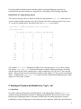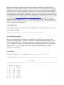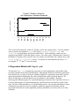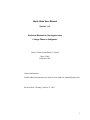
1
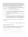
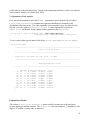
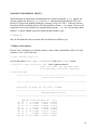
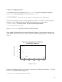
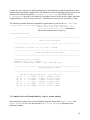
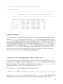
Haplo Stats User Manual
Version 1.1.0
Statistical Methods for Haplotypes when
Linkage Phase is Ambiguous
Jason P. Sinnwell and Daniel J. Schaid
Mayo Clinic
Rochester, MN
Contact Information:
Send feedback and questions by email to Jason Sinnwell, [email protected].
Revision Date: Monday, October 27, 2003
1
Table of Contents
1
Brief Description _________________________________________________________ 3
2
Operating System and Installation___________________________________________ 3
3
New Features ____________________________________________________________ 3
4
Getting Started ___________________________________________________________ 4
5
Preview for Missing Data by “summary.geno” _______________________________ 5
6
Haplotype Frequency Estimation by “haplo.em” _____________________________ 6
6.1 Algorithm_____________________________________________________________ 6
6.2 Example usage _________________________________________________________ 7
6.3 Control Parameters for “haplo.em” ______________________________________ 9
6.4 Haplotype Frequencies by Group Subsets ____________________________________ 10
7
Haplotype Score Tests by “haplo.score”___________________________________ 11
7.1
7.2
7.3
7.4
7.5
7.6
7.7
7.8
7.9
8
Quantitative Trait Analysis _______________________________________________ 12
Ordinal Trait Analysis ___________________________________________________ 13
Binary Trait Analysis____________________________________________________ 14
Plots and Haplotype Labels _______________________________________________ 15
Skipping Rare Haplotypes ________________________________________________ 16
Haplotype Scores, Adjusted for Covariates ___________________________________ 16
Permutation p-values ____________________________________________________ 17
Combine Score and Group Results by “haplo.score.merge” ________________ 18
Apply Score Tests to Sub-haplotypes by “haplo.score.slide” ______________ 19
Regression Models with “haplo.glm” ______________________________________ 21
8.1
8.2
8.3
8.4
8.5
Setting up the data.frame _____________________________________________ 22
Regression for a Quantitative Trait _________________________________________ 22
Fitting Haplotype x Covariate Interactions ___________________________________ 23
Regression for a Binomial Trait____________________________________________ 24
Control Parameters and Genetic Models _____________________________________ 25
9
License and Warranty _____________________________________________________ 27
10
Acknowledgements _______________________________________________________ 27
11
Appendix: Counting haplotype pairs when marker phenotypes have missing alleles _ 28
12
References_______________________________________________________________ 30
2
1 Brief Description
Haplo Stats is a suite of S-PLUS/R routines for the analysis of indirectly measured haplotypes. The
statistical methods assume that all subjects are unrelated and that haplotypes are ambiguous (due to
unknown linkage phase of the genetic markers). The genetic markers are assumed to be
codominant (i.e., one-to-one correspondence between their genotypes and their phenotypes), and so
we refer to the measurements of genetic markers as genotypes. The main functions in Haplo Stats
are:
haplo.em
....................... for the estimation of haplotype frequencies, and posterior probabilities of haplotype
pairs for a subject, conditional on the observed marker data
haplo.glm
....................... glm regression models for the regression of a trait on haplotypes, possibly including
covariates and interactions
haplo.score
....................... score statistics to test associations between haplotypes and a wide variety of traits,
including binary, ordinal, quantitative, and Poisson.
IMPORTANT NOTE: If you have used the previously distributed package for
haplo.score, it is important to note that the function haplo.score has
changed dramatically from the previous distribution, including the parameters
passed to this function. Please follow the examples provided in this document to see
how to use this function.
2 Operating System and Installation
Haplo Stats version 1.2.0 library is written for S-PLUS version 6.0 on a Unix operating system. It
is also translated to a library for R version 1.7.1. Installation procedures for both the S-PLUS and
R systems are in the README.haplo.stat file, which is included with the software distribution.
Once the library is installed and attached to a working directory, the procedures for running
analyses are the same for S-PLUS and R.
3 New Features
1. Accounting for missing genotypes: The first version (1.0) of haplo.score removed
subjects who were missing any marker genotypes. The current Haplo Stats functions allow for
missing marker genotypes.
2. Improved EM algorithm for estimating haplotype frequencies (see section 6.1).
3
3. Haplotype frequencies by subsets: Another new feature provides estimated haplotype
frequencies for subsets defined by levels of a qualitative ”group” variable (see the new function
haplo.group). This information can be combined with output from haplo.score by the
new function haplo.score.merge. These new functions are useful for case-control studies
in order to align estimates of haplotype frequencies for cases and controls with the
corresponding score statistics.
4. Regression models: The function haplo.glm is a major new addition, which provides a way
to regress a trait on haplotypes, covariates, and possibly their interactions.
4 Getting Started
After installing the Haplo Stats package, the routines and an example data set are available by
starting an S-PLUS or R session and attaching the appropriate directory. The easiest way to get
started is by following an example. An experienced user may want to skip the example and simply
view the details in the help files. As illustrated in the following example session, a user enters the
indented text following the prompt ">", and the output results follow.
Example Data
First attach the directory with the Haplo Stats routines and example data set (hla.demo). To do
this, use the local library concept, and type
> library(haplo.stats, lib.loc="/Installation Directory Path Here/")
where "/Installation Directory Path Here/" is the directory path that leads to the
directory haplo.stats. If using R, the example data is not yet accessible, so source the data into
the session by typing
> source(”/Installation Directory Path Here/haplo.stats/data/hla.demo.q”)
Now look at the names of variables in hla.demo.
> names(hla.demo)
[1]
[7]
[13]
[19]
[25]
"resp"
"DPA.a1"
"TAP1.a1"
"DQA.a1"
"A.a1"
"resp.cat"
"DPA.a2"
"TAP1.a2"
"DQA.a2"
"A.a2"
"male"
"DMA.a1"
"TAP2.a1"
"DRB.a1"
"age"
"DMA.a2"
"TAP2.a2"
"DRB.a2"
"DPB.a1"
"DMB.a1"
"DQB.a1"
"B.a1"
"DPB.a2"
"DMB.a2"
"DQB.a2"
"B.a2"
The variables are defined as follows:
resp
quantitative antibody response to measles vaccination
resp.cat a factor with levels "low", "normal", "high", for categorical antibody response
4
male
age
sex code with 1="male" , 0="female"
age (months) at immunization
The remaining variables are genotypes for 11 HLA loci, with a prefix name (e.g., "DQB") and a
suffix for each of two alleles (".a1" and ".a2").
The variables in hla.demo can be accessed by typing hla.demo$ before their names, such as
hla.demo$resp. Alternatively, it is easier to attach hla.demo, so the variables can be
accessed by simply typing their names.
> attach(hla.demo)
Creating a geno matrix
Many of the functions require a matrix of genotypes, denoted here as geno. This matrix is
arranged such that each locus has a pair of adjacent columns of alleles, and the order of columns
corresponds to the order of loci on a chromosome. If there are K loci, then the number of columns
of geno is 2*K. Rows represent the alleles for each subject. For example, if there are three loci, in
the order A-B-C, then the 6 columns of geno would be arranged as (A,a,B,b,C,c). For
illustration, three of the loci in hla.demo will be used to demonstrate some of the functions.
Create a separate data frame for 3 of the loci, and call this geno.
> geno <- hla.demo[,c(17,18,21:24)]
Create some labels for the loci.
> label <-c("DQB","DRB","B")
Random Numbers and Setting Seed
Simulations are used in several of the functions (e.g., to determine random starting values for
haplo.em, and to compute permutation p-values in haplo.score). In order to reproduce
results in this user guide, you must set the .Random.seed before any function which uses
random numbers. We illustrate this below, and it appears throughout the script UserManTest.q, but
we do not illustrate it throughout this user guide, to avoid clutter. In practice, the user would not
ordinarily reset the seed.
seed <- c(17, 53, 1, 40, 37, 0, 62, 56, 5, 52, 12, 1)
set.seed(seed)
5 Preview for Missing Data by “summary.geno”
Before running the haplotype statistics, the user may want to look for missing genotype data, to
determine the completeness of the data. If many genotypes are missing, the functions may take a
long time to compute results, and the user may want to remove some of the subjects with a lot of
missing data. This can be accomplished with the function summary.geno. This function checks
5
for missing allele information and counts the number of potential haplotype pairs that are
consistent with the observed data (see Appendix for a description of this counting algorithm).
IMPORTANT: Coding Missing Alleles
The codes for missing values of alleles are defined by the parameter miss.val, which may be a
vector to define multiple missing value codes. Because it has been common practice to use a zero
“0” to code for missing alleles, the default values for miss.val are 0 and NA.
> geno.desc <- summary.geno(geno, miss.val=c(0,NA))
> print(geno.desc)
1
2
3
.
.
.
80
81
82
83
.
.
.
135
136
137
138
.
.
.
loc miss-0 loc miss-1 loc miss-2 num_enum_rows
3
0
0
4
3
0
0
4
3
0
0
4
3
2
3
3
0
0
0
0
0
1
0
0
4
1800
2
1
3
3
1
3
0
0
0
0
0
0
2
0
4
2
129600
4
The columns “loc miss” illustrate the number of loci missing either 0, 1, or 2 alleles, and the
last column, num_enum_rows, illustrates the number of pairs of haplotypes that are consistent
with the observed data. In the example above, subjects indexed by rows 81 and 137 have missing
alleles. Subject #81 has one locus missing two alleles, while subject #137 has two loci missing two
alleles. As indicated by num_enum_rows, subject #81 has 1,800 potential haplotype pairs, while
subject #137 has nearly 130,000.
6 Haplotype Frequency Estimation by “haplo.em”
6.1 Algorithm
For genetic markers measured on unrelated subjects, with linkage phase unknown, haplo.em
computes maximum likelihood estimates of haplotype probabilities. Because there may be more
than one pair of haplotypes that are consistent with the observed marker phenotypes, posterior
probabilities of pairs of haplotypes for each subject are also computed. Unlike the usual EM which
6
attempts to enumerate all possible pairs of haplotypes before iterating over the EM steps, this
"progressive insertion" algorithm progressively inserts batches of loci into haplotypes of growing
lengths, runs the EM steps, trims off pairs of haplotypes per subject when the posterior probability
of the pair is below a specified threshold, and then continues these insertion, EM, and trimming
steps until all loci are inserted into the haplotype. The user can choose the batch size. If the batch
size is chosen to be all loci, and the threshold for trimming is set to 0, then this reduces to the usual
EM algorithm. The basis of this progressive insertion algorithm is from the sofware “snphap” by
David Clayton. (http://www-gene.cimr.cam.ac.uk/clayton/software/). Although some of the
features and control parameters of haplo.em are modeled after snphap, there are substantial
differences, such as extension to allow for more than two alleles per locus, and some other nuances
on how the algorithm is implemented.
6.2 Example usage
This example uses the geno matrix for the 3 loci defined above, which contains the two subjects
with some missing alleles.
> haplo.em(geno=geno, locus.label=label, miss.val=c(0,NA))
Note on missing genotypes
Because of the missing data, the number of possible pairs of haplotypes is quite large, which
increases the computation time. With the two subjects with missing genotypes included, it took
308.4 seconds of CPU time to complete the computations. If these two subjects are excluded, it
took 1.4 seconds of CPU time. It is a good idea to preview the data for missing values using the
function summary.geno. If there are just a few subjects with missing alleles, it may be
worthwhile to exclude them.
Print Method
To view the results in save.em, type either save.em or print(save.em):
> print(save.em)
================================================================================
Haplotypes
================================================================================
1
2
3
4
5
6
7
8
9
10
DQB DRB B hap.freq
21
1 8 0.00232
21
2 7 0.00227
21
2 18 0.00227
21
3 8 0.10401
21
3 18 0.00234
21
3 35 0.00570
21
3 44 0.00381
21
3 45 0.00227
21
3 49 0.00227
21
3 57 0.00227
7
.
.
.
================================================================================
Details
================================================================================
lnlike = -1846.856494
lr stat for no LD = 570.205143 , df =
123 , p-val =
0
Explanation of Results
The haplotypes and their estimated frequencies are listed, as well as a few details. The “lr stat
for no LD” is the likelihood ratio statistic contrasting the lnlike for the estimated haplotype
frequencies versus the lnlike assuming that alleles from all loci are in linkage equilibrium.
Trimming by the progressive insertion algorithm can invalidate the lr stat and the degrees of
freedom (df) – see the help file for haplo.em.
Summary Method
The function summary is used to see the list of haplotypes per subject, and their posterior
probabilities:
> summary(save.em)
================================================================================
Subjects: Haplotype Codes and Posterior Probabilities
================================================================================
subj.id hap1code hap2code posterior
1
1
76
54
1.00000
2
2
13
140
0.15586
3
2
17
135
0.84414
4
3
25
163
1.00000
5
4
13
36
1.00000
6
5
51
91
1.00000
7
6
4
17
1.00000
8
7
174
135
1.00000
9
8
134
49
1.00000
10
9
151
139
1.00000
.
.
.
460
217
166
31
1.00000
461
218
101
4
1.00000
462
219
4
124
1.00000
463
220
97
135
1.00000
================================================================================
8
Number of haplotype pairs: max vs used
================================================================================
1 2 84 133
1 18 0 0
0
2 51 3 0
0
4 121 25 0
0
1800
0 0 1
0
129600
0 0 0
1
Explanation of Results
The first part of summary lists the subject id (row number of input geno matrix), the codes for
the haplotypes of each pair, and the posterior probabilities of the haplotype pairs. The second part
gives a table of the maximum number of pairs of haplotypes per subject, versus the number of pairs
used in the final posterior probabilities.
The haplotype codes remove the clutter of illustrating all the alleles of the haplotypes, but may not
be as informative as the actual haplotypes themselves. To see the actual haplotypes, use the
show.haplo=T option:
> summary(save.em, show.haplo=T)
================================================================================
Subjects: Haplotype Codes and Posterior Probabilities
================================================================================
X76
X13
X17
X25
X131
X51
X4
X174
X134
X151
X96
.
.
.
subj.id hap1.DQB hap1.DRB hap1.B hap2.DQB hap2.DRB hap2.B posterior
1
32
4
62
31
11
61
1.00000
2
21
7
7
62
2
44
0.15586
2
21
7
44
62
2
7
0.84414
3
31
1
27
63
13
62
1.00000
4
21
7
7
31
7
44
1.00000
5
31
11
51
42
8
55
1.00000
6
21
3
8
21
7
44
1.00000
7
64
13
63
62
2
7
1.00000
8
61
13
44
31
11
44
1.00000
9
63
2
7
62
2
35
1.00000
10
51
1
27
51
1
35
1.00000
6.3 Control Parameters for haplo.em
An additional argument can be passed to haplo.em, called “control”. This is a list of
parameters that control the EM algorithm based on progressive insertion of loci. The default values
are set up by a function called haplo.em.control (see the help file for this function for a
complete description). Although the user can accept the default values, there are times when they
9
may need to be adjusted. For example, for small sample sizes and many possible haplotypes,
finding the global maximum of the log-likelihood can be difficult. The algorithm uses multiple
attempts to maximize the log-likelihood, starting each attempt with random starting values. If the
results from haplo.em, haplo.score, or haplo.glm change when rerunning the analyses, this may be
due to different maximizations of the log-likelihood. To avoid this, the user can increase the
number of attempts (n.try) to maximize the log-likelihood, increase the batch size
(insert.batch.size), or decrease the trimming threshold for posterior probabilities
(min.posterior). If the EM algorithm fails to converge, try increasing the maximum number
of iterations (max.iter). These parameters are defined below:
insert.batch.size: Number of loci to be inserted in a single batch.
min.posterior: Minimum posterior probability of haplotype pair, conditional on observed
marker genotypes. Posteriors below this minimum value will have their pair of
haplotypes "trimmed" off the list of possible pairs.
max.iter: Maximum number of iterations allowed for the EM algorithm before it stops and
prints an error.
n.try: Number of times to try to maximize the lnlike by the EM algorithm. The first try will
use, as initial starting values for the posteriors, either equal values or uniform
random variables, as determined by random.start. All subsequent tries will use
uniform random values as initial starting values for the posterior probabilities.
The example below illustrates how to set the number of trys to 20, and maximum number of
iterations to 1,000:
> save.em <- haplo.em(geno=geno, locus.label=label, miss.val=c(0, NA),
control=haplo.em.control(n.try = 20, max.iter = 1000) )
6.4 Haplotype Frequencies by Group Subsets
To compute the haplotype frequencies for each level of a grouping variable, use the function
haplo.group. The following example illustrates the use of a binomial response, y.bin to
create subsets, along with the geno matrix (see section 7.3 for creation of y.bin):
> group.bin <- haplo.group(y.bin, geno, locus.label=label, miss.val=0)
> print(group.bin)
-------------------------------------------------------------------------Counts per Grouping Variable Value
--------------------------------------------------------------------------
10
0 1
157 63
-------------------------------------------------------------------------Haplotype Frequencies By Group
-------------------------------------------------------------------------1
2
3
4
5
6
7
8
9
10
11
12
.
.
28
29
30
.
.
.
DQB DRB B
Total y.bin.0 y.bin.1
21
1 8 0.00232 0.00335
NA
21 10 8 0.00181 0.00318
NA
21 13 8 0.00274
NA
NA
21
2 18 0.00227 0.00318
NA
21
2 7 0.00227 0.00318
NA
21
3 18 0.00457 0.00637
NA
21
3 35 0.00571 0.00639
NA
21
3 44 0.00378 0.00333 0.00830
21
3 49 0.00227
NA
NA
21
3 57 0.00227
NA
NA
21
3 70 0.00227
NA 0.00794
21
3 8 0.10407 0.06973 0.19011
31
31
31
11 35 0.01753 0.01982 0.01587
11 37 0.00699 0.00661 0.00794
11 38 0.00699 0.00661 0.00794
Explanation of Results
The group.bin object can be very large, depending on the number of possible haplotypes, so
only a portion of the output is illustrated above. The first section gives a short summary of how
many subjects appear in each of the groups. The second section is a table with the following
columns:
• The first column gives row numbers.
• The next columns (3 in this example) illustrate the alleles of the haplotypes.
• Total are the estimated haplotype frequencies for the entire data set.
• The last columns are the estimated haplotype frequencies for the subjects in the levels of
the group variable (y.bin=0 and y.bin=1 in this example). Note that some
haplotype frequencies have an “NA”, which occurs when the haplotypes do not occur in
the subgroups.
7 Haplotype Score Tests by “haplo.score”
The function haplo.score is used to compute score statistics to test associations between
haplotypes and a wide variety of traits, including binary, ordinal, quantitative, and Poisson. This
function provides several different global and haplotype-specific tests for association, allows for
adjustment for non-genetic covariates, and optionally allows computation of permutation p-values
11
(which may be needed for sparse data). Details on the background and theory of the score statistics
can be found in Schaid et al. (Schaid et al. 2002).
7.1 Quantitative Trait Analysis
First, analyze the quantitative trait called resp. A quantitative trait is identified by the option
trait.type="gaussian" (a reminder that a gaussian distribution is assumed for the
distribution of the error terms). The other arguments, all set to default values, are defined in the
help file, viewed by typing help(haplo.score). To make reproducible output from
haplo.score, set the seed for the random number generator using set.seed().
> score.gaus <- haplo.score(resp, geno, trait.type="gaussian",
+
skip.haplo=.005, locus.label=label, simulate=F)
To view results, either type the name of the object, score.gaus, or print(score.gaus).
> print(score.gaus)
-------------------------------------------------------------------------Global Score Statistics
-------------------------------------------------------------------------global-stat = 46.20224, df = 38, p-val = 0.16957
-------------------------------------------------------------------------Haplotype-specific Scores
-------------------------------------------------------------------------[1,]
[2,]
[3,]
[4,]
[5,]
[6,]
[7,]
[8,]
[9,]
[10,]
.
.
.
DQB
21
21
31
63
62
51
63
33
31
63
DRB
3
7
4
13
2
1
13
7
11
2
B
8
13
44
60
35
44
44
57
44
7
Hap-Freq
0.10407
0.01076
0.02853
0.00575
0.00752
0.0173
0.01606
0.00682
0.01065
0.01334
Hap-Score
-2.39547
-2.30079
-2.24529
-1.75667
-1.2091
-0.99343
-0.84453
-0.58522
-0.53191
-0.50843
p-val
0.0166
0.0214
0.02475
0.07897
0.22663
0.3205
0.39837
0.5584
0.59479
0.61115
Explanation of Results
The section Global Score Statistics prints results for testing an overall association
between haplotypes and the response. The global-stat has an asymptotic χ2 distribution, with
degrees of freedom df and p-value as indicated.
12
Haplotype-specific Scores are given in a table format. The column descriptions are as
follows:
The first column gives row numbers.
The next columns (3 in this example) illustrate the alleles of the haplotypes.
Hap-Freq is the estimated frequency of the haplotype in the pool of all subjects.
Hap-Score is the score for the haplotype.
p-val is the asymptotic chi-square (1 df) p-value.
In our example, the option simulate=F in the function haplo.score implied no permutation
p-values (permutation p-values are computed when simulate=T.) Note that this table is sorted
according to Hap-Score.
7.2 Ordinal Trait Analysis
To create an ordinal trait, convert resp.cat (a factor with levels "low", "normal", "high") to
numeric values, y.ord (with levels 1, 2, 3).
> y.ord <- as.numeric(resp.cat)
Now use the option trait.type = "ordinal"
> score.ord <- haplo.score(y.ord, geno, trait.type="ordinal",
+
offset = NA, x.adj = NA, skip.haplo=.005,
+
locus.label=label, miss.val=0, simulate=F)
> print(score.ord)
-------------------------------------------------------------------------Global Score Statistics
-------------------------------------------------------------------------global-stat = 62.14589, df = 38, p-val = 0.00801
-------------------------------------------------------------------------Haplotype-specific Scores
-------------------------------------------------------------------------[1,]
[2,]
[3,]
[4,]
[5,]
[6,]
.
.
.
DQB DRB B Hap-Freq
21
7 13 0.01076
21
3
8 0.10407
31
4 44 0.02853
63 13 60 0.00575
33
7 57 0.00682
33
9 60 0.00682
Hap-Score
-3.67054
-2.79161
-2.61709
-2.35844
-0.93375
-0.93375
p-val
0.00024
0.00524
0.00887
0.01835
0.35043
0.35043
13
WARNING FOR ORDINAL TRAITS:
When analyzing an ordinal trait with adjustment for covariates (using the x.adj option), the
software requires the libraries Design and Hmisc, distributed by Frank Harrell, Ph.D. (see
Harrell, FE. Regression Modeling Strategies, Springer-Verlag, NY, 2001). If the user does not
have these libraries installed, then it will not be possible to use the x.adj option. However, the
unadjusted scores for an ordinal trait (using the default option x.adj=NA) do not require these
libraries. To check whether your local system has these libraries, type
> library()
and you should then be able to examine the list of libraries available to you.
7.3 Binary Trait Analysis
Because "low" responders are of primary interest, create a binary trait that has values of 1 when
response is "low", and 0 otherwise.
> y.bin <-ifelse(y.ord==1,1,0)
Now use the option trait.type = "binomial" in the haplo.score routine
> score.bin <- haplo.score(y.bin, geno, trait.type="binomial",
+
offset = NA, x.adj = NA, skip.haplo=.005,
+
locus.label=label, miss.val=0, simulate=F)
> print(score.bin)
-------------------------------------------------------------------------Global Score Statistics
-------------------------------------------------------------------------global-stat = 61.90705, df = 38, p-val = 0.00846
-------------------------------------------------------------------------Haplotype-specific Scores
-------------------------------------------------------------------------[1,]
[2,]
[3,]
[4,]
[5,]
[6,]
[7,]
[8,]
.
.
DQB
62
51
63
21
64
63
32
64
DRB
2
1
13
7
13
13
8
13
B
7
35
7
7
35
62
7
63
Hap-Freq
0.05091
0.03018
0.01655
0.01417
0.00897
0.00866
0.00682
0.00682
Hap-Score
-2.19135
-1.58423
-1.56008
-1.55906
-1.27328
-1.14173
-1.10475
-1.10475
p-val
0.02843
0.11314
0.11874
0.11898
0.20292
0.25357
0.26927
0.26927
14
7.4 Plots and Haplotype Labels
A convenient way to view results from haplo.score is a plot of the haplotype frequencies
(Hap-Freq) versus the haplotype score statistics (Hap-Score).
> plot(score.gaus)
> title("Figure 1. Haplotype Score Statistics\nQuantitative Response")
Some points on the plot may be of interest, perhaps due to their score statistic, or their haplotype
frequency. To put haplotype labels on individual points in the plot, use the function
locator.haplo. To use this feature, first type the following command:
> locator.haplo(score.gaus)
where score.gaus is the object where the results are stored.
Now, with the left mouse button, click on all the points of interest. After points are chosen, click
on the middle mouse button. All the points are labeled with their haplotype labels, as illustrated in
Figure 1.
Figure 1. Haplotype Score Statistics
Quantitative Response
2
1
0
−1
−2
Haploltype Score Statistic
•
•
• 32: 4:62
62: 2: 7
63:13: 7
•
• •
•
••
•
•
•
••
•• • •
•
••
••• • •
•
••
•
•
•
•
21: 7:13
•
31: 4:44
21: 3: 8
•
0.02
•
0.04
0.06
0.08
0.10
Haplotype Frequency
If some of the haplotype labels overlap, it may be necessary to clean up the coordinates. To do this,
save the x-y coordinates and haplotype text,
> loc.gaus <- locator.haplo(score.gaus)
15
and then fix some of the x-y coordinates in the loc.gaus list.
7.5 Skipping Rare Haplotypes
For the quantitative trait analyses, the option skip.haplo=.005 was used to pool all haplotypes
with frequencies < 0.005 into a common group. Now try a different cut-off, such as
skip.haplo=.01.
> score.gaus.01 <- haplo.score(resp, geno, trait.type="gaussian",
+
offset = NA, x.adj = NA, skip.haplo=.01,
+
locus.label=label, miss.val=0, simulate=F)
> print(score.gaus.01)
-------------------------------------------------------------------------Global Score Statistics
-------------------------------------------------------------------------global-stat = 33.20509, df = 20, p-val = 0.03203
-------------------------------------------------------------------------Haplotype-specific Scores
-------------------------------------------------------------------------[1,]
[2,]
[3,]
[4,]
[5,]
[6,]
[7,]
[8,]
.
.
.
DQB DRB B Hap-Freq
21
3
8 0.10407
21
7 13 0.01076
31
4 44 0.02853
51
1 44 0.0173
63 13 44 0.01606
31 11 44 0.01065
63
2
7 0.01334
21
7 44 0.02167
Hap-Score
-2.39547
-2.30079
-2.24529
-0.99343
-0.84453
-0.53191
-0.50843
-0.47268
p-val
0.0166
0.0214
0.02475
0.3205
0.39837
0.59479
0.61115
0.63644
Note that by using a different value for skip.haplo, the global statistic and its p-value change
(due to decreased df), but the haplotype-specific scores do not change.
7.6 Haplotype scores, adjusted for covariates
First set up a covariate matrix, with the first column for male (1 if male; 0 if female), and the
second column for age (in months).
> x.ma <- cbind(male, age)
16
Now use this matrix as an argument to haplo.score.
> score.gaus.adj <- haplo.score(resp, geno, trait.type="gaussian",
+
offset = NA, x.adj = x.ma, skip.haplo=.005,
+
locus.label=label, miss.val=0, simulate=F)
> print(score.gaus.adj)
-------------------------------------------------------------------------Global Score Statistics
-------------------------------------------------------------------------global-stat = 46.46501, df = 38, p-val = 0.16298
-------------------------------------------------------------------------Haplotype-specific Scores
-------------------------------------------------------------------------[1,]
[2,]
[3,]
[4,]
[5,]
[6,]
[7,]
[8,]
.
.
.
DQB DRB B Hap-Freq
21
3
8 0.10407
21
7 13 0.01076
31
4 44 0.02853
63 13 60 0.00575
62
2 35 0.00752
51
1 44 0.0173
63 13 44 0.01606
33
7 57 0.00682
Hap-Score
-2.40888
-2.29123
-2.25532
-1.77426
-1.2136
-0.98748
-0.83952
-0.60404
p-val
0.016
0.02195
0.02411
0.07602
0.2249
0.32341
0.40118
0.54582
When adjusting for covariates, all score statistics can change, although not by much in this
example.
7.7 Permutation p-values
Permutation p-values are computed when simulate=T. In addition to a global statistic, and
haplotype-specific statistics, a “max-stat” statistic, and corresponding permutation p-value, is
computed. The max-stat is the maximum among all haplotype-specific score statistics. Because
the distribution of this statistic is unknown, the p-value for max-stat is given only when
permutations are requested. If only a few haplotypes are associated with the trait, the max-stat
should have greater power than the global statistic.
The score.sim.control function manages simulation control parameters. Simulated
statistics are based on randomly permuting the trait and covariates (same order for both), but not
the geno matrix, and then computing the haplotype score statistics, adjusted for covariates.
haplo.score employs the simulation p-value precision criteria of Besag and Clifford (Besag
and Clifford 1991). These criteria ensure that the permutation p-values for both the global and the
maximum score statistics are precise for small p-values. The algorithm performs a user-defined
minimum number of permutations (min.sim) to guarantee sufficient precision for the simulated
17
p-values for score statistics for individual haplotypes. Permutations beyond this minimum are then
conducted until the sample standard errors for simulated p-values for both the global and max score
statistics are less than a threshold (p.threshold * p-value). The default value for
p.threshold=¼ provides a two-sided 95% confidence interval for the p-value with a width that
is approximately as wide as the p-value itself. Simulations are more precise for smaller p-values.
The following example illustrates computation of permutation p-values with min.sim=1000.
> score.bin.sim <- haplo.score(y.bin, geno, trait.type="binomial",
+
offset = NA, x.adj = NA, skip.haplo=.005,
+
locus.label=label, miss.val=0, simulate=T,
+
sim.control=score.sim.control())
> print(score.bin.sim)
-------------------------------------------------------------------------Global Score Statistics
-------------------------------------------------------------------------global-stat = 61.90705, df = 38, p-val = 0.00846
-------------------------------------------------------------------------Global Simulation p-value Results
-------------------------------------------------------------------------Global sim. p-val = 0.00561
Max-Stat sim. p-val = 0.00596
Number of Simulations, Global:
2853 , Max-Stat: 2853
-------------------------------------------------------------------------Haplotype-specific Scores
-------------------------------------------------------------------------[1,]
[2,]
[3,]
[4,]
[5,]
[6,]
.
.
.
DQB
62
51
63
21
64
63
DRB B Hap-Freq
2
7 0.05091
1 35 0.03018
13
7 0.01655
7
7 0.01417
13 35 0.00897
13 62 0.00866
Hap-Score
-2.19135
-1.58423
-1.56008
-1.55906
-1.27328
-1.14173
p-val
0.02843
0.11314
0.11874
0.11898
0.20292
0.25357
sim p-val
0.02769
0.12478
0.19593
0.11847
0.32878
0.36558
7.8 Combine Score and Group Results by “haplo.score.merge”
When analyzing a binary trait, it can be helpful to align the results from haplo.score with
haplo.group. To do so, use the function haplo.score.merge, as illustrated in the
following example:
18
> merge.bin <- haplo.score.merge(score.bin, group.bin)
> print(merge.bin)
-------------------------------------------------------------------------Haplotype Scores, p-values, and Frequencies By Group
-------------------------------------------------------------------------1
2
3
4
5
6
7
8
.
.
.
DQB DRB B Hap.Score
p.val Hap.Freq y.bin.0 y.bin.1
62
2 7 -2.19135 0.02843 0.05091 0.06790 0.01587
51
1 35 -1.58423 0.11314 0.03018 0.03755 0.00893
63 13 7 -1.56008 0.11874 0.01655 0.02182
NA
21
7 7 -1.55906 0.11898 0.01417 0.01968
NA
64 13 35 -1.27328 0.20292 0.00897 0.01318
NA
63 13 62 -1.14173 0.25357 0.00866 0.01274
NA
32
8 7 -1.10475 0.26927 0.00682 0.00955
NA
64 13 63 -1.10475 0.26927 0.00682 0.00955
NA
Explanation of Results
The first column is a row index, the next columns (3 in this example) illustrate the haplotype, the
column “Hap.Score” is the score statistic and “p.val” the corresponding chi-square p-value,
Hap.prob is the haplotype frequency for the total sample, and the remaining last two columns are
the estimated haplotype frequencies for each of the group levels (y.bin in this example). The
default print method only prints results for haplotypes appearing in the haplo.score output. To
view all haplotypes, use the print option all.haps=T, which prints records for all haplotypes
from the haplo.group output. The output is ordered by the score statistic, but the order.by
parameter can specify ordering by haplotypes or by haplotype frequency. See the help file for
print.haplo.score.merge for details on printing options.
7.9 Apply Score Tests to Sub-haplotypes by “haplo.score.slide”
To evaluate the association of sub-haplotypes (subsets of alleles from the full haplotype) with a
trait, the user can evaluate a “window” of alleles by haplo.score, and slide this window across
the entire haplotype. This procedure is implemented by the function haplo.score.slide. To
illustrate this method, we use all 11 loci in the demo data, hla.demo.
First, make the geno matrix and the locus labels for the 11 loci.
> geno.11 <- hla.demo[,-c(1:4)]
> label.11 <- c("DPB","DPA","DMA","DMB","TAP1","TAP2","DQB","DQA","DRB","B","A")
Now use haplo.score.slide for a window of 3 loci (n.slide=3), which will slide along
the haplotype for all 9 contiguous subsets of size 3, using the same gaussian trait as above.
19
> score.slide.gaus <- haplo.score.slide(resp, geno.11, trait.type="gaussian",
n.slide=3, skip.haplo=.005, locus.label=label.11)
> print(score.slide.gaus)
1
2
3
4
5
6
7
8
9
start.locus score.global.p score.global.p.sim score.max.p.sim
1
0.2953181
NA
NA
2
0.0078272
NA
NA
3
0.2270697
NA
NA
4
0.7650744
NA
NA
5
0.2173284
NA
NA
6
0.2112196
NA
NA
7
0.2178192
NA
NA
8
0.0283782
NA
NA
9
0.0486047
NA
NA
Explanation of Results
The first column is the row index of the nine calls to haplo.score, the second column is the
number of the starting locus of the sub-haplotype, the third column is the global score statistic pvalue. The last two columns are the simulated p-values for the global and maximum score
statistics, respectively. If simulate=T was specified in the function call, the simulated p-values
would be present.
Plot Results from haplo.score.slide
The results from haplo.score.slide can be easily viewed in a plot, by the command
> plot(score.slide.gaus,cex=.6)
> title("Figure 2. Global p-values for\n sub-haplotypes; Gaussian
Response",cex=.6)
with results illustrated in Figure 2.
20
1.5
1.0
0.5
0.0
−log10(score.global.p)
2.0
Figure 2. Global p−values for
sub−haplotypes; Gaussian Response
A
B
DRB
DQA
DQB
TAP2
TAP1
DMB
DMA
DPA
DPB
The x-axis has tick marks for each locus, and the y-axis is the -log10(p-value). To select which pvalue to plot, use the parameter pval, with choices “global”, “global.sim”, and
“max.sim” corresponding to p-values described above. If the simulated p-values were not
computed, the default is to plot the global p-values. For each p-value, a horizontal line is drawn at
the height of -log10(p-value) across the loci over which it was calculated. For example, the p-value
score.global.p = 0.0078272 for loci 2-4 will plot as a horizontal line plotted at y=2.1
covering the 2nd, 3rd, and 4th x-axis tick marks.
8 Regression Models with “haplo.glm”
The function haplo.glm computes the regression of a trait on haplotypes, and possibly other
covariates and their interactions with haplotypes. Although this function is based on a generalized
linear model, only two types of traits are currently supported: 1) quantitative traits with a normal
(gaussian) distribution and identity link, and 2) binomial traits with a logit-link function. The
effects of haplotypes on the link function can be modeled as either additive, dominant
(heterozygotes and homozygotes for a particular haplotype assumed to have equivalent effects), or
recessive (homozygotes of a particular haplotype considered to have an alternative effect on the
trait). The basis of the algorithm is a two-step iteration process; the posterior probabilities of pairs
of haplotypes per subject are used as weights to update the regression coefficients, and the
regression coefficients are used to update the posterior probabilities. See Lake (Lake et al. 2003)
for details.
21
8.1 Setting up the data.frame
A critical distinction between haplo.glm and all other functions in Haplo Stats is that the
definition of the regression model follows the S-PLUS/R formula standard. So, a data.frame
must be defined, and this data.frame must contain the trait, a special kind of genotype matrix
(called geno in this example) that contains the genotypes of the marker loci, and possibly other
covariates and weights for the subjects. The key feature of this data.frame is how geno is
defined. In order to keep the columns of geno as a single unit when inserting into a data.frame
(and not separate columns of the data.frame), the geno matrix must be defined as a
model.matrix. The following steps in S-PLUS are necessary to convert geno to the
appropriate model.matrix:
> geno <- as.matrix(hla.demo[,c(17,18,21:24)])
> oldClass(geno) <- "model.matrix"
In R, one would use class instead of oldClass:
> class(geno) <- "model.matrix"
Now create a data.frame for the regressions
my.data <- data.frame(geno, age=hla.demo$age, male=hla.demo$male,
y=hla.demo$resp, y.bin=y.bin)
8.2 Regression for a Quantitative Trait
The following illustrates how to fit a regression of quantitative trait y on the haplotypes defined by
the matrix geno, and the covariate male. The control parameter, haplo.freq.min, is
discussed below under the heading Explanation of Results, as well as in section 8.5.
> fit.gaus <- haplo.glm(y ~ male + geno, family = gaussian,
data=my.data, locus.label=label, control =
haplo.glm.control(haplo.freq.min = 0.02))
To view the results of a model fit, type either the name of the saved object (e.g., fit.gaus), or
use print:
> print(fit.gaus)
> fit.gaus
Call:
haplo.glm(formula = y ~ male + geno, family = gaussian, data = my.data,
na.action = "na.geno.keep", locus.label = locus.label, control =
haplo.glm.control(haplo.freq.min = 0.02))
22
Coefficients:
coef
se t.stat
pval
(Intercept) 1.0661 0.343 3.109 0.001067
male 0.0973 0.155 0.627 0.265575
geno.16 0.2534 0.453 0.560 0.288125
geno.35 -0.3187 0.343 -0.928 0.177171
geno.77 0.2226 0.361 0.616 0.269229
geno.78 1.1401 0.384 2.971 0.001658
geno.99 0.5539 0.364 1.521 0.064897
geno.137 0.9836 0.303 3.241 0.000692
geno.rare 0.3971 0.182 2.183 0.015052
Haplotypes:
DQB DRB B hap.freq
geno.16 21
7 44
0.0213
geno.35 31
4 44
0.0286
geno.77 32
4 60
0.0302
geno.78 32
4 62
0.0239
geno.99 51
1 35
0.0301
geno.137 62
2 7
0.0502
geno.rare
*
* *
0.7117
haplo.base 21
3 8
0.1041
Explanation of Results
The above table for Coefficients lists the estimated value (coef), its standard error (se), the
corresponding t-statistic (t.stat) , and p-value (pval). The labels for haplotype coefficients are
a paste of the matrix defining the genotypes (geno in the above example) and the haplotype
numbers. The haplotypes corresponding to these haplotype numbers are listed in the above table
under Haplotypes, along with the estimates of the haplotype frequencies (hap.freq). The rare
haplotypes (those with frequencies less than haplo.freq.min, 0.02 in the above example) are
pooled into a single category labeled rare. The haplotype chosen as the base-line category for the
design matrix (most frequent haplotype is the default) is labeled as haplo.base.
8.3 Fitting Haplotype x Covariate Interactions
Interactions are fit by the usual model syntax, using a “*” to indicate main effects and interactions,
> fit.inter <- haplo.glm(y ~ male * geno, family = gaussian,
data=my.data, locus.label= label, control
= haplo.glm.control(haplo.freq.min =
0.02))
> fit.inter
Call:
haplo.glm(formula = y ~ male * geno, family = gaussian, data = my.data,
na.action = "na.geno.keep", locus.label = label, control =
haplo.glm.control(haplo.freq.min = 0.02))
Coefficients:
(Intercept)
coef
se
0.9804 0.303
t.stat
pval
3.2385 0.000701
23
male
geno.16
geno.35
geno.77
geno.78
geno.99
geno.137
geno.rare
malegeno.16
malegeno.35
malegeno.77
malegeno.78
malegeno.99
malegeno.137
malegeno.rare
0.2535
0.0925
-0.1749
0.8032
0.4931
0.5197
1.1601
0.4529
0.5522
-0.2783
-0.8967
1.2660
0.0540
-0.4491
-0.0956
0.314
0.462
0.596
0.591
0.489
0.400
0.354
0.182
0.720
0.667
0.698
0.655
0.661
0.521
0.206
0.8081
0.2003
-0.2937
1.3588
1.0092
1.2992
3.2800
2.4841
0.7673
-0.4170
-1.2847
1.9330
0.0816
-0.8627
-0.4634
0.209988
0.420724
0.384661
0.087854
0.157044
0.097668
0.000610
0.006896
0.221897
0.338571
0.100183
0.027308
0.467516
0.194645
0.321770
Haplotypes:
DQB DRB B hap.freq
geno.16 21
7 44
0.0219
geno.35 31
4 44
0.0285
geno.77 32
4 60
0.0305
geno.78 32
4 62
0.0241
geno.99 51
1 35
0.0301
geno.137 62
2 7
0.0504
geno.rare
*
* *
0.7103
haplo.base 21
3 8
0.1041
Explanation of Results
The listed results are as explained under section 8.2. The only difference is that the interaction
coefficients are labeled as a paste of the covariate (male in this example) and the name of the
haplotype.
8.4 Regression for a Binomial Trait
The following illustrates the fitting of a binomial trait:
> fit.bin <- haplo.glm(y.bin ~ male + geno, family = binomial, data=my.data,
locus.label= label, x=T, control =
haplo.glm.control(haplo.freq.min = 0.02))
> print(fit.bin)
Call:
haplo.glm(formula = y.bin ~ male + geno, family = binomial, data = my.data,
na.action = "na.geno.keep", locus.label = locus.label, control =
haplo.glm.control(haplo.freq.min = 0.02), x = T)
Coefficients:
(Intercept)
male
geno.16
geno.35
geno.77
geno.78
geno.99
geno.137
coef
1.539
-0.480
-0.569
0.370
-0.997
-1.403
-2.582
-2.717
se
0.420
0.324
0.702
0.623
0.690
0.773
0.708
0.759
t.stat
3.666
-1.480
-0.811
0.595
-1.447
-1.814
-3.646
-3.580
pval
1.56e-04
7.02e-02
2.09e-01
2.76e-01
7.48e-02
3.55e-02
1.68e-04
2.13e-04
24
geno.rare -1.261 0.253 -4.980 6.59e-07
Haplotypes:
DQB DRB B hap.freq
geno.16 21
7 44
0.0215
geno.35 31
4 44
0.0284
geno.77 32
4 60
0.0306
geno.78 32
4 62
0.0235
geno.99 51
1 35
0.0298
geno.137 62
2 7
0.0518
geno.rare
*
* *
0.7104
haplo.base 21
3 8
0.1040
Interpreting Results for a Binomial Trait
The underlying methods for haplo.glm are based on a prospective likelihood. Normally, this
type of likelihood works well for case-control studies with standard covariates. For ambiguous
haplotypes, however, one needs to be careful when interpreting the results from fitting haplo.glm to
case-control data. Because cases are over-sampled, relative to the population prevalence (or
incidence, for incidence cases), haplotypes associated with disease will be over-represented in the
case-control sample, and so estimates of haplotype frequencies will be biased. Positively associated
haplotypes will have haplotype frequency estimates that are higher than the population haplotype
frequency. To avoid this problem, one can weight each subject. The weights for the cases should be
the population prevalence, and the weights for controls should be 1 (assuming the disease is rare in
the population, and controls are representative of the general population). See Stram (Stram et al.
2003) for background on using weights, and see the help file for haplo.glm for how to
implement weights with haplo.glm.
The estimated regression coefficients for case-control studies can be biased by either a large
amount of haplotype ambiguity and mis-specified weights, or by departures from Hardy Weinberg
equilibrium of the haplotypes in the pool of cases and controls. Generally, the bias is small, but
tends to be towards the null of no association. See Stram (Stram et al. 2003) and Epstein (Epstein
and Satten 2003) for further details.
8.5 Control Parameters and Genetic Models
A key parameter for haplo.glm is control, which is a list of parameters that control the
procedures of haplo.glm. This control list is set up by the function haplo.glm.control.
A parameter of this control function is haplo.effect, which instructs whether the haplotype
effects are fit as additive, dominant, or recessive. That is, haplo.effect determines whether the
covariate (x) coding of haplotypes is "additive" (causing x = 0, 1, or 2, the count of a particular
haplotype), "dominant" (causing x = 1 if heterozygous or homozygous carrier of a particular
haplotype; x = 0 otherwise), or "recessive" (causing x = 1 if homozygous for a particular haplotype;
x = 0 otherwise).
> fit.dom <- haplo.glm(y ~ male + geno, family = gaussian,
data=my.data, locus.label=label,
control = haplo.glm.control(haplo.effect = dom,
25
haplo.freq.min = 0.02) )
The other control parameter used above, haplo.freq.min, is the minimum haplotype
frequency required for a haplotype to be included in the regression model as its own effect.
See the help file for haplo.glm.control for further control parameters.
26
9 License and Warranty
License:
Copyright 2003 Mayo Foundation for Medical Education and Research.
This program is free software; you can redistribute it and/or modify it under the terms of
the GNU General Public License as published by the Free Software Foundation; either
version 2 of the License, or (at your option) any later version.
This program is distributed in the hope that it will be useful, but WITHOUT ANY
WARRANTY; without even the implied warranty of MERCHANTABILITY or
FITNESS FOR A PARTICULAR PURPOSE. See the GNU General Public License for
more details.
You should have received a copy of the GNU General Public License along with this
program; if not, write to the Free Software Foundation, Inc., 59 Temple Place, Suite 330,
Boston, MA 02111-1307 USA
For other licensing arrangements, please contact Daniel J. Schaid.
Daniel J. Schaid, Ph.D.
Division of Biostatistics
Harwick Building – Room 775
Mayo Clinic
200 First St., SW
Rochester, MN 55905
phone: 507-284-0639
fax:
507-284-9542
email: [email protected]
10 Acknowledgements
This research was supported by United States Public Health Services, National Institutes of Health;
Contract grant numbers R01 DE13276, R01 GM 65450, N01 AI45240, and R01 2AI33144. The
hla.demo data is kindly provided by Gregory A. Poland, M.D. and the Mayo Vaccine Research
Group for illustration only, and may not be used for publication.
27
11 Appendix: Counting haplotype pairs when marker phenotypes have
missing alleles
The following describes the process for counting the number of haplotype pairs that are
consistent with a subject's observed marker phenotypes, allowing for some loci with missing data.
Note that we refer to marker phenotypes, but our algorithm is oriented towards typical markers that
have a one-to-one correspondence with their genotypes. We first describe how to count when none
of the loci have missing alleles, and then generalize to allow loci to have either one or two missing
alleles. When there are no missing alleles, note that homozygous loci are not ambiguous with
respect to the underlying haplotypes, because at these loci the underlying haplotypes will not differ
if we interchange alleles between haplotypes. In contrast, heterozygous loci are ambiguous,
because we do not know the haplotype origin of the distinguishable alleles (i.e., unknown linkage
phase). However, if there is only one heterozygous locus, then it doesn’t matter if we interchange
alleles, because the pair of haplotypes will be the same. In this situation, if parental origin of
alleles were known, then interchanging alleles would switch parental origin of haplotypes, but not
the composition of the haplotypes. Hence, ambiguity arises only when there are at least two
heterozygous loci. For each heterozygous locus beyond the first one, the number of possible
haplotypes increases by a factor of 2, because we interchange the two alleles at each heterozygous
locus to create all possible pairs of haplotypes. Hence, the number of possible haplotype pairs can
be expressed as 2 x , where x = H − 1 if H (the number of heterozygous loci) is at least 2, otherwise
x = 0.
Now consider a locus with missing alleles. The possible alleles at a given locus are
considered to be those that are actually observed in the data. Let ai denote the number of
distinguishable alleles at the i th locus. To count the number of underlying haplotypes that are
consistent with the observed and missing marker data, we need to enumerate all possible genotypes
for the loci with missing data, and consider whether the imputed genotypes are heterozygous or
homozygous.
To develop our method, first consider how to count the number of genotypes at a locus, say
th
the i locus, when either one or two alleles are missing. This locus could have either a
homozygous or heterozygous genotype, and both possibilities must be considered for our counting
method. If the locus is considered as homozygous, and there is one allele missing, then there is
only one possible genotype; if there are two alleles missing, then there are ai possible genotypes. A
function to perform this counting for
homozygous loci is denoted f ( ai ) .
Table 1. Number of possible genotypes at a locus with
missing alleles according to whether the genotype is
If the locus is considered as
homozygous or heterozygous.
heterozygous, and there is one allele
missing, then there are ai − 1
Number of
Homozygous
Heterozygous
possible genotypes; if there are two
missing alleles
function,
function,
alleles missing, then there are
f ( ai )
g ( ai )
ai ( ai − 1) / 2 possible genotypes. A
1
1
ai − 1
function to perform this counting for
2
ai
ai ( ai − 1) / 2
heterozygous loci is denoted g ( ai ) .
These functions and counts are
summarized in Table 1.
28
Now, to use these genotype counting functions to determine the number of possible
haplotype pairs, first consider a simple case where only one locus, say the i th locus, has two
missing alleles. Suppose that the phenotype has H heterozygous loci (H is the count of
heterozygous loci among those without missing data). We consider whether the locus with missing
data is either homozygous or heterozygous, to give the count of possible haplotype pairs as
ai 2 x + [ai ( ai − 1) / 2] 2 x +1 ,
where again x = H − 1 if H is at least 2, otherwise x = 0. This special case can be represented by
our more general genotype counting functions as
f ( ai ) 2 x + g ( ai ) 2 x +1 .
When multiple loci have missing data, we need to sum over all possible combinations of
heterozygous and homozygous genotypes for the incomplete loci. The rows of Table 2 below
present these combinations for up to m=3 loci with missing data. Note that as the number of
heterozygous loci increases (across the columns of Table 2), so too does the exponent of 2. To
calculate the total number of pairs of haplotypes, given observed and possibly missing genotypes,
we need to sum the terms in Table 2 across the appropriate row. For example, with m = 3, there are
eight terms to sum over. The general formulation for this counting method can be expressed as
m
Total Pairs = ∑
∑ C (combo, i )
i = 0 combo
where combo is a particular pattern of heterozygous and homozygous loci among the loci with
missing values (e.g., for m = 3, one combination is the first locus heterozygous and the second and
third as homozygous), and C ( combo, i ) is the corresponding count for this pattern when there are i
loci that are heterozygous (e.g., for m = 3 and i = 1, g ( a1 ) f ( a2 ) f ( a3 ) 2 x +1 , as illustrated in Table 2).
Table 2. Summands to count the number of pairs of haplotypes consistent with observed marker
phenotypes when there are m loci with missing alleles.
Number of loci with missing alleles that are considered as heterozygous
0
1
2
3
m
0
2x
1
f ( a1 ) 2 x
g ( a1 ) 2 x +1
2
f ( a1 ) f ( a2 ) 2 x
g ( a1 ) f ( a2 ) 2 x +1
g ( a1 ) g ( a2 ) 2 x + 2
f ( a1 ) g ( a2 ) 2 x +1
3
f ( a1 ) f ( a2 ) f ( a3 ) 2 x
g ( a1 ) f ( a2 ) f ( a3 ) 2 x +1
g ( a1 ) g ( a2 ) f ( a3 ) 2 x +2
f ( a1 ) g ( a2 ) f ( a3 ) 2 x +1
g ( a1 ) f ( a2 ) g ( a3 ) 2 x +2
f ( a1 ) f ( a2 ) g ( a3 ) 2 x +1
f ( a1 ) g ( a2 ) g ( a3 ) 2 x +2
g ( a1 ) g ( a2 ) g ( a3 ) 2 x +3
29
12 References
Besag J, Clifford P (1991) Sequential Monte Carlo p-Values. Biometrika 78:301-304
Epstein M, Satten G (2003) Inference on haplotype effects in case-control studies using unphased
genotype data. Submitted
Lake S, Lyon H, Silverman E, Weiss S, Laird N, Schaid D (2003) Estimation and tests of
haplotype-environment interaction when linkage phase is ambiguous. Human Heredity
55:56-65
Schaid DJ, Rowland CM, Tines DE, Jacobson RM, Poland GA (2002) Score tests for association
between traits and haplotypes when linkage phase is ambiguous. Am J Hum Genet 70:42534
Stram D, Pearce C, Bretsky P, Freedman M, Hirschhorn J, Altshuler D, Kolonel L, Henderson B,
Thomas D (2003) Modeling and E-M estimation of haplotype-specific relative risks from
genotype data for case-control study of unrelated individuals. Hum Hered To Appear
30