Download On-Chip Thermoelectric Cooling Tool

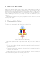
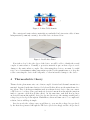
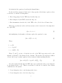
On-Chip Thermoelectric Cooling Tool
’User manual’
David Saenz
March 28, 2011
1
Introducion
Thermoelectricity is the study of the relationship between heat and electrical energy. There
are two main thermoelectric effects, one on which a heat current through a thermocouple
produces an electrical current (Seebeck effect) and one on which an electrical current produces a heat current (Peltier effect). Thermoelectric devices make use of these two effects
to either produce power out of a temperature gradient, or generate a temperature difference
between the two sides of the device by the use of electrical power. This simulation tool is
intended to exemplify one of the main applications of the Peltier effect. A thermoelectric
cooler or heat pump (commonly known as Peltier cell) is localized on the top of a microprocessor’s casing. Then, a heat sink is attached right on the top of it (this is a common layout
on cooling applications). The Peltier cell will take heat from the chip and pump it towards
the heat sink which dissipates it to the ambient when an electric current is made to flow
trough it.
We can compare the way this Peltier cooler works with a common refrigerator. We
spend some amount of electrical energy to transport heat from one place to another. We
can measure the process efficiency by taking the ratio of the useful work performed (heat
being removed) to the energy expenditures. This efficiency is commonly represented by
a Coefficient of Performance (COP). In common Peltier devices, this is very small, which
means that we would have to invest a lot of energy to move a small amount of heat from
one side to the other. This is why they are only used in applications where heir use is
imprescindible. Otherwise, we can recur to a common gas compression refrigerator or other
air conditioning systems. Cooling a chip with these devices is an example on which we need
of these devices due to its small size, durability and maintenance free feature.
1
2
How to use this manual
While science underlying thermoelectrics is quite complex, in this manual you will find an
initial perspective of one of the applications of a thermoelectric cooler by keeping most of the
intrincacies apart. And although an explanation of the formulas and the code embedded in
this tool is provided in this manual, it has to be noted that these are only approximations to
what it actually happens, and it is a good example of a real life case, which is the objective
of the tool.
This manual is presented as a step by step explanation on how to use the tool, as well
as interpret the outputs.
3
Thermoelectric Device
The layout of a common single-couple Peltier device is shown below:
Figure 1: Thermoelectric Heat Pump
This picture explains how this cooling business works. The process can be outlined as
follows:
1. Cooper connects the n- and p-type semiconductor materials electrically in series and
thermally in parallel.
2. Current flows through the circuit in the direction indicated to transfer heat from the
top part to the bottom part.
Common Peltier devices are made of several of this junction connected electrically in
series and thermally in parallel, as shown in the picture below:
2
Figure 2: Peltier Cell Schematic
The contacts and semiconductor materials are sandwiched in between two slabs of insulating material (commonly ceramic). A real life device is shown below:
Figure 3: Real Peltier Device
If we take a close look to the edges of the device, we will be able to identify the several
couples of semiconductor. Normally, a protective material is put on these edges to avoid
damage to the semiconductor couples. Also, when using these devices, one must be careful
not to exceed a maximum working temperature specified by the manufacturer so to keep the
soldier connecting the device from being melt, or other irreversible damage to the device.
4
Thermoelectric theory
Thermoelectric phenomena arise out of inter-coupled electrical and thermal currents in a
material. As stated in the introduction, Seebeck and Peltier effects are the main thermoelectric effects. They both happen simultaneously in a thermoelectric device. One can connect
a TE device to a voltage source and make an electrical current flow through the junctions
inside to generate a heat flow (Peltier effect). At the same time, such heat flow produces
an electrical current through the device (in opposite direction to the existing current) and a
voltage drop is developed throughout. Furthermore, this would turn out to be a complicated
relation, but we will keep it simple.
In a few words, the voltage source would have to overcome the voltage drop produced
by the heat flow generated through the TE device (Seebeck voltage) and the one produced
3
by the actual device to make current flow. This process will dissipate heat according to the
ohm’s law; W = V ∗ I. Other heat source would be the chip power dissipation (Qte ). Then
one can map the heat currents through the layout ad come up with equations describing the
flow of heat.
Let’s start with a simple one-couple device:
Figure 4: Thermoelectric Heat Pump (Dual Semiconductor Pellet)
For each metal-semiconductor-metal junction (two in the above figure):
Heat will be pumped from the hot side according to the formula
q = πI
(1)
Where q can be called the ’heat current’ and π is the peltier coefficient, which describes
the amount of heat current per unit charge. I is just the electric current through the
materials.
In turn, while powering the device, the power dissipated as heat flows half towards the
hot side and half towards the cooled side. This is simple joule heat described by ohm’s law
as:
I 2R
(2)
But we find convenient to express the electrical resistance R as a function of the geometrical dimensions of the thermocouples. Assuming the p- and n-type elements within the TEC
are the same shape and size and neglecting contact resistance, we can express the electrical
resistance of the single pellet cooler module as:
R = ρ(length/area) = ρ/G
4
(3)
where ρ stands for the electrical resistivity of the semiconductor material. And although
in reality, n- and p-type pellets have different ρ, we will assume uniformity between both.
Also we will call the ratio of the area to length of the element gamma factor (G) for simplification.
The last heat contribution to the system is the one generated by the voltage drop due
to the Seebeck voltage through the TEC. It is easily calculated by multiplying this thermoelectrically generated voltage by the total current flowing through the device, (V ∗ I):
QV.Seebeck = Iα∆T
(4)
Where α is the Seebeck coefficient and ∆T is the difference in temperature between the
hot and cold side of the TE device (heated and cooled respectively). I is again the electrical
current that flows through the TEC.
Now that we have found the heat current through the system and explained how the
single-coupled TEC works, we can turn our attention to the simulation and the math.
5
Simulation
Thermal resistances are present within a junction of two objects. These resistances will
make heat not to flow uniformly through the components and will develop a change in
temperature. This is what we are interested in, knowing the temperatures at the different
stages of our layout. If we want to know the temperature at a certain point on the system,
we just need to multiply the heat current at the interested stage, by the thermal resistance
at the corresponding junction.
This process can be compared to electrical circuit calculations. One can take heat current
as being electrical current, voltage at a resistance as the temperature of the junction, and
electrical resistances as thermal resistances (we can use this analogy due to the 1D system
assumption). As an example, lets take the heat current flowing from the TEC to the heat sink
q and multiply it by the thermal resistance between that specific junction. The result would
yield the junction temperature, just as multiplying the electrical current times an electrical
resistance yields the voltage drop across it. To find the temperature at the heat sink-ambient
junction, we would just have to add the ambient temperature to the temperature resulting
by multiplying the thermal resistance in the heat-sink to ambient junction and we are good!
Now we can come up with heat balance equations describing the temperature at each
section of our layout.
In the application mentioned in the introduction, the TE cooler (TEC) is put in between
the chip case and the heat sink as shown below:
5
Figure 5: Chip Layout
Heat flows from the chip to the case, then it is pumped through the peltier device, and
then dissipated by the heat sink. Some assumptions are made in this case:
1. One dimensional system.
2. Heat flows only due to conduction processes.
3. Temperature is absolute and invariable on each part of the setup.
4. Temperature independent thermoelectric parameters.
5. No thermal resistance between electrical junctions within the TEC.
6. No thermal masses; instant heat transmission (no transient state).
The image below shows the heat currents through the device and the thermal resistances
at the junctions:
Figure 6: Thermal Profile
Heat currents are the big red arrows, each labeled with a number on the tail (1 and
2). Thermal resistances are represented as electrical resistances through the diagram. The
temperature at each junction can be found by multiplying the total heat current through the
junction by the corresponding thermal resistance and adding the corresponding temperature
from the past junction.
6
Let’s first find the equations describing the thermal fluxes.
For the total heat current # 1 (the total cooling capacity of the thermocouple), we have
to take into account the following fluxes:
1. Heat being pumped by the TEC away from the chip case.
2. Heat dissipated by the TEC towards the chip case.
3. Heat transmission from hot side of the TEC to the cold side due to Fourier’s law.
Thus if we say that Qm is the total heat current on the bottom side of the single thermocouple TEC,
Qm = 1 + 2 + 3
(5)
And multiplying by the number of thermocouples, the equation becomes
Qm = 2N (1 + 2 + 3)
(6)
Where:
1. = αTc I
2. = −I 2 ρ/2G
3. = −kG(Th − Tc )
Where Tc and Th are the cold and the hot side of the TEC respectively and k is the
thermal conductivity of the thermoelectric elements. The negative side indicates backflow
of heat. And we get our first equation for heat current looking something like this:
Qm = 2N (αTc I − I 2 ρ/2G − kG(Th − Tc ))
(7)
Now let’s analyze the flux after the TEC. Let’s say now that Qte is the power dissipated
by the thermoelectric cooler. Thus we would have to take into account two heat current
contributions to the system:
1. Power dissipation due to joule heating in the device.
2. Power dissipation due to Seebeck voltage drop.
7
Just as before, we have to multiply the total addition of the fluxes by the number of
thermocouples. The equation for the TEC heat contribution would then look like:
Qte = 2N (1 + 2)
(8)
Where:
1. = I 2 ρ/G
2. = αI(Th − Tc )
And we get our second equation for heat current:
Qte = 2N (I 2 ρ/G + αI(Th − Tc ))
(9)
Now we just need to calculate the localized temperatures at each of the interfaces by
multiplying the corresponding flux addition times each thermal resistance and adding any
preexisting heat.
Equations would look like:
1. Qm = 2N (αTc I − I 2 ρ/2 ∗ G − kG(Th − Tc ))
2. Qte = 2N (I 2 ρ/G + αI(Th − Tc ))
3. Tchip = Tc + Qm (Rchip−case + Rcase−T EC )
4. Thot = T0 + (Qm + Qte )(RT EC−H.Sink + RH.Sink−Amb )
Here, in equation 2, we multiplied the thermal resistances Rchip−case + Rcase−T EC by its
corresponding thermal current and then added the temperature at the cold side of the TEC
to get the total temperature at the chip junction. Similarly, to find the temperature at the
hot side of the TEC, we multiply the thermal resistances RT EC−H.Sink + RH.Sink−Amb times
the corresponding heat current and then add the ambient temperature.
Analyzing these equations, we realize that there are four unknowns, Th , Tc , Tchip and
Qte . The user can fix Qm and I on the simulation. Thus, a system of four equations and
four unknowns is developed. The recommended method to solve this system is by using the
”rref” (row reduce echelon form) function from MatLab once the corresponding matrix has
been found. Below, the code used to solve these equations is shown.
8
Matrix = [(2*N*(alpha*I+K*G))
0
0
(Qm+N*I^2*rho/G);
(-2*N*alpha*I) 1
0
(2*N*I^2*rho/G);
0
1
-(R2 + R3))
0
(T0 + Qm*(R2 + R3));
-1
0
0
1
(Qm*(R0+R1))];
(2*N*alpha*I)
(-2*N*K*G)
M = rref(Matrix);
This would yield the result for each of the variables for given values of Qm and I. A full
copy of the code is available under request.
6
Input & Output
Default values are set for a common device. There are three categories for user input.
1. TEC characteristics.
2. Thermal Resistances.
3. Analysis Type.
Each of them is briefly discussed below.
6.1
TEC Characteristics
• No. of N-P couples.- This is the number of thermoelectric n- and p-type material
couples in the Peltier cell.
• Seebeck Coefficient.- This is the coefficient of proportionality indicating how much
voltage is generated through the device per temperature difference. Units are in volts
per kelvin(V/K)
• Electrical Resistivity.- An average resistivity of n- and p-type materials. In units
of ohm per meter (ohm*m).
• Gamma Factor.- The ratio of a thermoelectric element ( single cube of semiconductor
element) to its length. In units of meters (m).
9
• Thermal Conductivity.- A measure of the ability of the TEC to transfer heat per
unit time, given one unit area and the temperature gradient through the thickness of
the device. In units of watts per meter per degree Kelvin (W/m-K).
6.2
Thermal Resistances
In here the user specifies the thermal resistances of each of the junctions in the device in
units of degree kelvin per Watt (K/W).
• Chip to Case.
• Case to TEC.
• TEC to Heat Sink.
• Heat Sink to Ambient.
6.3
Analysis Type
• Analysis.- Here the user can choose whether to sweep for maximum cooling capacity
or current input to the TEC.
• Ambient Temperature.- The temperature of the heat sink surroundings in degrees
Kelvin (K).
• Current Feed.- Current through TEC (only for Sweep Power Dissipation analysis)
in units of Amperes (A).
• Power Dissipation.- The maximum power pumped out of the chip (only for Sweep
Current Input analysis) in units of Watts (W).
• Maximum Plot Range.- Maximum range for each kind of simulation.
• Minimum Plot Range.- Minimum range when plotting in sweep current mode.
6.4
Output
There is a graph for each of the variables in the equations solved earlier in the manual. There
is also a plot of the temperature difference across the TEC labeled as Thot Tcold, as well as
one for the figure of merit of the device. Below summary of output graphs.
1. Cold Side Temperature of the TEC.
10
2. Hot Side Temperature of the TEC.
3. Thot-Tcold.
4. Chip Temperature.
5. Power Dissipated by the TEC.
6. Figure of Merit.
Each of these graphs is self explanatory.
References
[1] D. K. C. MacDonald, Thermoelectricity an introduction to the principles. Dover, New
York, 1st Edition, 2006.
[2] Mark Lundstrom, Thermoelectric Nanotechnology. https://nanohub.org/resources/9421,
2010.
[3] TXL Group Inc, Thermoelectric Generation Developer’s Kit. TXL Group Inc., Texas,
1st Edition, 2009.
11