Download ESCET Version β0.3 User Manual

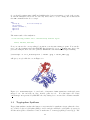
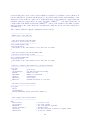
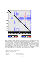
ESCET
Version β0.3
User Manual
Thomas R. Schneider
January 24, 2003
Contents
1 Introduction
2
2 Command Scripts and Data Structure
2.1 Atom sets . . . . . . . . . . . . . . . . . . . . . . . . . . . . . . . . . . . . . . . .
2.2 Atoms . . . . . . . . . . . . . . . . . . . . . . . . . . . . . . . . . . . . . . . . . .
2.3 Residues . . . . . . . . . . . . . . . . . . . . . . . . . . . . . . . . . . . . . . . . .
3
3
4
4
3 Identification of the rigid part of a protein
3.1 Chorismat Mutase . . . . . . . . . . . . . . . . . . . . . . .
3.2 Asparte Aminotransferase . . . . . . . . . . . . . . . . . . .
3.3 Tryptophan Synthase . . . . . . . . . . . . . . . . . . . . . .
3.4 Mersacidin . . . . . . . . . . . . . . . . . . . . . . . . . . .
3.5 Comparing models from non-identical but very homologeous
.
.
.
.
.
6
7
9
11
13
16
4 Utilities
4.1 Juggling pdb-files . . . . . . . . . . . . . . . . . . . . . . . . . . . . . . . . . . . .
4.2 Stuff . . . . . . . . . . . . . . . . . . . . . . . . . . . . . . . . . . . . . . . . . . .
18
18
19
5 Tips and Tricks
20
6 Release Notes
23
1
. . . . . .
. . . . . .
. . . . . .
. . . . . .
molecules
.
.
.
.
.
.
.
.
.
.
.
.
.
.
.
.
.
.
.
.
.
.
.
.
.
Chapter 1
Introduction
ESCET is a script driven program to analyse and compare three-dimensional protein structures.
The current β-test version is mostly for calculating and displaying error-scaled difference distance
matrices. Starting with version 0.2, an automatic algorithm to interpret difference distance
matrices has been added [6].
This document contains a short introduction to the program. The easiest way to get started
is to look through the different scenarios discussed in chapter 3 and use one of the examples
scripts.
Running the command ’escet -h’ from the unix-command line will create an html-file called
escet ref.html that can be used as a reference manual.
An ESCET-script file can be executed from the UNIX command line using a command of the
following form:
escet < myscript.inp > myscript.log &
Diagnostic output will then end up in myscript.log, graphical output will be dumped to a
postscript file. Scripts to look at the output using RASMOL and or molscript are put into
files called t ras.ras and t molscript.mol, respectively.
Currently, the program is only available as an executable for the Linux operating system.
If you find the program useful, please cite the following paper: Schneider TR: A genetic algorithm for the identification of conformationally invariant regions in protein molecules Acta Cryst
D58:195-208 (2002). Thank you.
Please report all problems to me (email: [email protected])
The program and its documentation are copyright Thomas R. Schneider (2000-02).
I would like thank the β-testers (in particular Karl Edman from Uppsala University) for putting
up with a semi-functional version of the program and for making lots of useful suggestions.
2
Chapter 2
Command Scripts and Data
Structure
The program stores data pertaining to atoms in ’atom sets’. An atom set can contain an almost
unlimited number of atoms, the number of sets is currently limited to 100. Atom sets can be
manipulated and analysed using a large number of commands. The commands are normally put
in a command script which is then run from a unix shell. A typical command script has the
form:
!
! ESCET-script for making a Bfactor-plot
!
! read information about atoms from pdb-file
! 2lzt.pdb into atom set number one.
aset_read(tset=0,ifile="2lzt.pdb");
! select atoms in residues 5 to 100. Use atom set
! number 0 as the source and atom set number 1 as the target
aset_sele(sset=0,tset=1,sele=(resi in 5-100));
! make a plot of the property ’bfac’ of the CA atoms
! vs. residue number for the atoms found in sset 1
rp_plot(sset=1,prop=bfac,aver=ca);
Some output will be printed to the screen, graphical output will be dumped to a postscript
file. Please not that the rp plot -command at the moment only works for proteins, and not for
RNA/DNA (but I am trying to fix this).
2.1
Atom sets
Atom sets represent the information that can be found for example in a pdb file. They are
basically a collection of atoms with some general information such as name of the protein or the
crystallographic unit cell found in the pdb file attached.
Information about atoms can be read from from various file formats. Currently supported
formats are: pdb, shelxl-.ins/.res, shelxl-.lst. As much information as possible is extracted
from the respective files, e.g. if an .lst file contains s.u.’s, these are stored.
Once atoms have been read, sets can be modified by applying selection criteria (command
aset select, keyword sele).
3
All commands related to sets of atoms have a syntax of the form aset *(); and are described
in the reference manual.
2.2
Atoms
Atoms are the ’elementary unit’ of the program. An atom has a number of properties that can
be used and modified. Examples of such properties are: x, y, z coordinates, atom name, chain
identifier, chemical element, B factor etc. pp..
2.3
Residues
In the framework of ESCET, a residue is a set of atoms that share the same chain identifier
and the same residue number. To count, a residue must have at least one atom named ’CA’. If
properties of entire residues (e.g. the average B factor of the sidechain atoms) have to be stored,
the information is kept with the respective Cα -atom.
2.3.1
Secondary structure information
A typical property of a residue is the type of secondary structure element it is located in. This
information is stored as a single letter in the atom property ssid (for secondary structure identifier). of the respective Cα -atom. The single letter code corresponds to the Kabsch&Sander
notation as for example used in PROCHECK. The codes and their meanings are given in Table 2.3.1.
code
’B’
’E’
’G’
’H’
’I’
’S’
’T’
’e’
’g’
’h’
’t’
’’
meaning
residue in isolated beta-bridge
extended strand, participates in beta-ladder
3-helix (3/10 helix)
4-helix (alpha-helix)
5-helix (pi-helix)
bend
hydrogen-bonded turn
extension of beta-strand
extension of 3/10 helix
extension of alpha-helix
used in PROCHECK, but I don’t know what it means
no secondary structure
Table 2.1: Identifiers used for secondary structure elements
If a pdb-file is read, the program will try to figure out the secondary structure assignment from
the HELIX and SHEET records. If you are reading the data from a non-pdb file, a pdb file
without the HELIX and SHEET records or if you are not happy with the assignment read, you
can modify the atom property ssid using the aset amod command. The two commands:
aset_amod(set=1,ssid=H,sele=(resi in {3-20:34-40}));
aset_amod(set=1,ssid=E,sele=(resi in {24-30:44-50}));
4
will modify the atoms in set 1 such that residues 3 to 20 and 34 to 40 will become α helical
and residues 24 to 30 and 44 to 50 will become β sheet.
5
Chapter 3
Identification of the rigid part of a
protein
Please,
try to roughly understand the paper on the subject: [6] before trying to run the program ...
As it stands now, the analysis of a set of conformers will proceed as follows:
1. Read a bunch of models from one (in the case of NCS-related molecules) or several coordinate files. → aset read()-command.
2. Select the atoms that will be analysed. Usually these will be Cα -atoms. In complicated
cases, one can also restrict selections to chainids and residue ranges etc. to obtain consistent sets of atoms. (the program tries to figure out the largest consistent set itself,
but sometimes needs a bit of help). → aset select()-command. In simple cases, the
selection can be done directly in the aset read()-command.
3. If no standard uncertainties have been read from the coordinate file (as is the case most of
the time, unless you are in the fortunate situation of having a shelxl lst-file from a fullmatrix inversion available), some estimates for the coordinate error have to be generated.
Normally one would use the B-factor scaled DPI (explained in [5]). → aset egen()command. The program is pretty clever in extracting the information it needs to calculate
the error estimates from the pdb-file. In case, not all the necessary pieces can be found,
the information can be added by hand (see section 3.2).
4. Run the automated error-scaled difference distance matrix analysis. → ddm()-command.
5. Look at the results in the log-file or use the automatically generated scripts for
lsqkab,molscript, and RASMOL, to create some more intuitive representations.
The following examples are discussed:
Chorismat Mutase (Section 3.1) Compare three NCS-related copies of Chorismat Mutase
at 1.3 Å. Make figures that can be used for publication in Acta Cryst. D. For more see [6].
6
Aspartate Aminotransferase (Section 3.2) Compare five different models of Aspartate
Aminotransferase. The models have been refined to different resolutions and some of
the information necessary to generate standard uncertainties has to added manually. For
more see [6].
Tryptophan Synthase (Section 3.3) Two models of Tryptophan Synthase are compared.
Both, normal and error-scaled difference distance matrices are displayed for comparison.
For more on this analysis, see [5].
Mersacidin (Section 3.4) How to display 36 matrices for two different ways of comparing 6
NCS-related molecules at once. For a change, estimated standard deviations are available
from a shelxl lst-file.
3.1
Chorismat Mutase
Comparison of three NCS-related molecules
Here is the script to read the data, divide the atoms into NCS-related copies and run the analysis.
!--------------------------------------! ESCET-script cmut_ddm_5.0.inp
!--------------------------------------! Read the structure, keep only CA-atoms
! -------------------------------------aset_read(ifile="1DBF.pdb",sele=(name == CA));
! Generate standard uncertainties based on the information
! found in the pdb-file. As the completeness of the data
! was not present in the pdb-file, so the value was put in
! manually.
! -------------------------------------------------------aset_egen(sset=0,esd_model=dpiu,cpl=92.0);
! divide the structure into three independent sets of atoms
! --------------------------------------------------------aset_sele(tset=1,sele=(chainid == A));
aset_sele(tset=2,sele=(chainid == B));
aset_sele(tset=3,sele=(chainid == C));
! calculate an plot the error-scaled difference distance
! matrices for all pairs of molecules
! ------------------------------------------------------ddm(
setl={1-3},
! list of atom sets to look at
esd_scaled=on,
! use error-scaling
lolim=5.0,hilim=10.0,
! limit for matrix
xtint = 50,
! ticks suitable for publication
ticksfontsize = 14,
! font suitable for Acta after shrinking
ssplot=on,
! plot secondary structure
rb_plot=on,
! plot rigid body description
pstype=ps,
! produce an ps-file on output
psfname="cmut_ddm_5.0.ps"
! filename for graphics
);
7
! finito
stop();
To run this script, type:
> escet < cmut_ddm_5.0.inp > cmut_ddm_5.0.out
This will dump the difference distance matrices into a file called cmut ddm 5.0.ps. You can
look at this file with ghostview if your are interested. Otherwise you can check out the log-file
cmut ddm 5.0.out. Most interesting is probably the graphical representation of the results: files
called t ras.ras and t molscript.mol have been created that can be used to show the results
using RASMOL and molscript respectively.
Typing:
% rasmol -script t_ras.ras
will bring up a nice little RASMOL -window displaying your molecule with the conformationally
invariant atoms in blue and the flexible ones in red (see Figure 3.1.a).
(a)
(b)
Figure 3.1: (a) RASMOL-display of a molecule of Chorismate Mutase with rigid parts mapped
onto the molecule in blue, flexible parts in red. (b) The same with molscript.
Typing
% molscript -r < t_molscript.mol | render -jpeg > t_molscript.jpg
will produce a rendered molscript plot (See Figure 3.1.b). Of course, you may need to put the
correct coordinate transformation into the molscript-input file first. If you have the openglversion of molscript, this is very easy.
8
There is also a script to run the CCP4-program lsqkab on the different structures:
t lsqkab.csh. As such a superposition can be quite complicated, the script is also a bit complicated and may need some editing - I have tried to put some useful comments into this script.
But sometimes the script even works without editing ... Then simply run it from the command
line (after changing there permissions to executable, of course: % chmod +x t lsqkab.csh.
WARNING: All the scripts that start with t will be overwritten relentlessly by
subsequent runs of ESCET in the same directory. So, if you want to safe these
scripts, rename them !
In the first run, lolim = l = 5σ was used as a lower limit for significant changes. To rerun
the whole thing with a different setting of l = 2σ, all we have to do, is to change the lolimparameter of the ddm-keyword and rerun the program.
The bit that is interesting in the log-file, can be found by searching the log-file for the string
’conformationally invariant region’. Here, the program tells us what it has identified as
conformationally invariant:
==> The following residues form a conformationally invariant region:
A3-A13, A48-A52, A86-A95.
There is some more useful stuff in that part of the file - have a look around.
3.2
Asparte Aminotransferase
Here we read five models from five different files. As the pdb-files are a bit of a mess, we have
to put some of the numbers necessary for the calculation of uncertainties by hand:
!--------------------------------------! ESCET-script aatase_ddm1.inp
!--------------------------------------! Read the models, keep only CA-atoms and take only
! the first chain, if there are several chains
! ------------------------------------------------aset_read(tset=1,ifile="7AAT.pdb",sele=((name == CA) and
aset_read(tset=2,ifile="1TAR.pdb",sele=((name == CA) and
aset_read(tset=3,ifile="1AMA.pdb",sele=((name == CA)));
aset_read(tset=4,ifile="1TAS.pdb",sele=((name == CA) and
aset_read(tset=5,ifile="1TAT.pdb",sele=((name == CA) and
!
!
!
!
!
(chainid == A)));
(chainid == A)));
(chainid == A)));
(chainid == A)));
Generate standard uncertainties for all models. For none
of the models, all the necessary information can be found
in the pdb-file ... So we have put in various numbers
manually (from the files or from the paper)
----------------------------------------------------------
! 7AAT
aset_egen(sset=1,esd_model=dpiu,dmin=1.9,npar=27968);
! 1TAR
aset_egen(sset=2,esd_model=dpiu,nobs=36893,npar=26320,cpl=88.5,dmin=2.2);
! AMA
aset_egen(sset=3,esd_model=dpiu,dmin=2.3,npar=13892,nobs=17538,cpl=94.4,);
9
! 1TAS
aset_egen(sset=4,esd_model=dpiu,npar=25408,nobs=17636,cpl=87.9,rfree=30.0,dmin=2.8);
! 1TAT
aset_egen(sset=5,esd_model=dpiu,npar=25408,nobs=18194,cpl=97.0,dmin=3.0,rfree=30.0);
ddm(
setl={1-5},
esd_scaled=on,
lolim=2.0,hilim=5.0,
ssplot=on,
rbplot=on
);
stop();
The first run on all the models is used to decide which conformers are identical. For this purpose,
a table is printed in the log-file:
Pairwise Comparison of entire models:
------------------------------------The following table contains for every pair of models the percentage of
elements in the error-scaled difference distance matrix that are smaller
than the threshold value of lolim = 2.00. If for a pair of models, this value
is larger than 98.0%, the two models can be considered to be identical.
For an explanation see T.R. Schneider, Acta Cryst D58, in the press (2002).
7AAT
7AAT
1TAR
1AMA
1TAS
1TAT
*100.0*
73.3
76.3
82.0
81.9
84.5
86.8
*100.0*
*100.0*
1TAR
1AMA
1TAS
*100.0*
1TAT
The above table can be used to decide which conformers are redundant and
should not be included in the rigid-body analysis in order to not overweight
such conformers. If, for a group of conformers, all matrix elements are
larger than 98.0%, a good way to continue is to only include the conformer
with the lowest average esd into the subsequent analysis
Here, for the groups of (7AAT, 1TAR) and (1AMA, 1TAS, 1TAT), the matrix elements indicate
that the respective conformers are the same within experimental error.
To find the most precise representative of each group, we can consult another table:
Some statistics for atomlists to be analysed:
---------------------------------------------->
-->
-->
-->
-->
AL[1]
AL[2]
AL[3]
AL[4]
AL[5]
<esd>
<esd>
<esd>
<esd>
<esd>
=
=
=
=
=
0.107
0.326
0.252
0.299
0.403
+/+/+/+/+/-
0.048
0.048
0.149
0.194
0.299
from
from
from
from
from
0.030
0.222
0.041
0.041
0.051
to
to
to
to
to
10
0.502
0.550
1.460
2.057
2.567
’7AAT.pdb
’1TAR.pdb
’1AMA.pdb
’1TAS.pdb
’1TAT.pdb
->
->
->
->
->
401
401
402
402
401
sel.’
sel.’
sel.’
sel.’
sel.’
So, we should continue using 7AAT and 1AMA as the best representative of each of the groups.
To run the analysis for those two models only, all we have to do is to change the atoms sets in
the ddm-command in the above script:
ddm(
setl={1:3},
# <== was setl={1-5}
esd_scaled=on,
lolim=2.0,hilim=5.0,
ssplot=on,
rbplot=on
);
The main result of the analysis is:
==> The following residues form a conformationally invariant region:
A4-A12, A47-A226, A232-A328.
Now you can use the corresponding Cα -atoms in your favourite fitting program. You can also
try to use the lsqkab-script that ESCET has generated for you: t lsqkab.csh. As for the
previous examples, there are some premade RASMOL- and molscript-scripts. Running
% molscript -r -in t_molscript.mol | render -jpeg > aatase_ddm2.jpg
will give you a plot like the one in Figure 3.2.
Figure 3.2: molscript-figure of a molecule of Aspartate Aminotransferase with rigid parts
mapped onto the molecule in blue, flexible parts in red.
For this figure the script
t molscript.mol generated by ESCET- the only editing done concerned the orientation matrix.
3.3
Tryptophan Synthase
Tryptophan synthase catalyses the last two reactions in the biosynthesis of tryptophan, the cleavage of indole 3-glycerol phosphate (IGP) to indole and glyceraldehyde 3-phosphate (α-reaction)
and the subsequent condensation of indole with serine to form tryptophan (β-reaction) [3]. The
11
reactions take place at two active centers which are separated by a distance of more than 25 Å,
but nevertheless are precisely synchronized [1]. In a study aimed at the understanding of the
interaction between the two active sites, crystal structures of the enzyme in complex with the
substrate analogue 5-fluoroindole propanol phosphate (TRPSF-IPP , pdb-entry 1A50) and in
complex with both F-IPP and L-serine (TRPSF-IPP
, where ’A-A’ stands for the amino-acrylate
A-A
that is formed at the β-site under the experimental conditions chosen; pdb-entry 1A5S) were
determined [7].
The complete difference distance analysis is described in [5].
!----------------------------! ESCET-script: trps_ddm1.inp
!----------------------------! read the structure with IPP bound
! and select the bits that we want
! ---------------------------------aset_read(ifile=1A50.pdb);
aset_select(tset=1,
sele=((name == CA) and (chainid == "B") and (resi in 3-389))
);
! read the structure with IPP and AMAC bound
! and select the bits that we want
! -------------------------------------------aset_read(ifile=1A5S.pdb);
aset_select(tset=2,
sele=((name == CA) and (chainid == "B") and (resi in 3-389))
);
! generate coordinate uncertainties for the first structure
! --------------------------------------------------------aset_egen(
sset=1,
! atom set #1
esd_model=dpiu,
! use DPI plus linear B-scaling
ni=5191,
! number of atoms
nobs=31627,
! number of observables
cpl=95.6,
! completeness
rfree=22.1,
! free R-value
dmin=2.29
! maximum resolution of x-ray data
);
! the same for the second structure
! --------------------------------aset_egen(
sset=2,
esd_model=dpiu,
ni=5148,nobs=30327,cpl=93.8,rfree=24.7,dmin=2.30
);
! first display error-scaled matrix
! --------------------------------ddm(
seta=1,setb=2,
esd_scaled=on,
rbfind=off,
lolim=1.5,hilim=5.0,
type=lower,
comments=off,
!
!
!
!
!
!
atom sets to use
use error-scaling
don’t run genetic algorithm
display limits
use only lower half of matrix to display result
do not put comments
12
pstype=eps,
psfname=trps_ddm1.eps,
title="DD matrices for TRPS",
ssplot=on
);
! now display normal matrix
! ------------------------ddm(
seta=1,setb=2,
esd_scaled=off,
lolim=0.3,hilim=2.0,
type=upper,
);
!
!
!
!
make an eps-file
name of eps-file
put a title
put secondary structure scheme
!
!
!
!
atom sets to use
this time no error-scaling
display limits
use only upper half for display
! plot a black diagonal
! --------------------ddm(seta=1,setb=2,type=diag);
stop();
This script produces the plot shown in Figure 3.3
3.4
Mersacidin
Mersacidin is a polypeptide antibiotic containing 20 amino-acids that crystallizes with six
molecules in the asymmetric unit. The structure was solved and refined against merohedrally
twinned data to 1.06 Å resolution as described in [5]. The conformations of the six molecules are
similar to each other with a mean rmsd for all 15 possible pairwise least-squares superpositions
(using all Cα atoms) of 0.83 Å, as calculated by LSQKAB [4]. Analysis of the superimposed
molecules to identify rigid and flexible regions was inconclusive.
For six molecules, there are ((6 × 6) − 6)/2 = 15 possible pairwise comparisons. The analysis of
the corresponding 15 difference distance matrices allowed the indentification of rigid and flexible
parts of the molecule. The analysis is described in [5].
For the six atom sets corresponding to the six molecules, all possible pairwise difference distance
matrices can be plotted (on 15 pages of paper) using the following script:
! ------------------------------! ESCET-script: ddm_mers_all.inp
! ------------------------------! read coordinates and errors from SHELXL list file
! keep only CA-atoms
! -----------------aset_read(ifile = ./mers_fin_ls.lst,sele=(name == CA));
! prepare six atom sets, one for each molecule
! -------------------------------------------aset_select(tset=1,sele=(name == CA) and (resi
aset_select(tset=2,sele=(name == CA) and (resi
aset_select(tset=3,sele=(name == CA) and (resi
aset_select(tset=4,sele=(name == CA) and (resi
aset_select(tset=5,sele=(name == CA) and (resi
aset_select(tset=6,sele=(name == CA) and (resi
in
in
in
in
in
in
13
101-120));
201-220));
301-320));
401-420));
501-520));
601-620));
3
50
100
150
200
250
300
350
389
3
50
−5.0 σ−1.5 σ
100
150
200
1.5 σ 5.0 σ
250
300
−2.0 Å −0.3 Å
350
0.3 Å
389
2.0 Å
Figure 3.3: Difference distance matrix between the structures of tryptophan synthase in complex
with F-IPP (TRPSF-IPP ) and in complex with F-IPP and amino-acrylate (TRPSF-IPP
). In the
A-A
lower left half, the error-scaled difference distance matrix is displayed using upper and lower
cutoffs of 1.5 and 5.0σ, respectively. In the upper right half, the ordinary difference matrix is
displayed using a lower cutoff of 0.3 Å corresponding to approximately the 1σ level as determined
by the σA -method. For scaling, an upper cutoff of 2.0 Å has been employed. Both matrices
underwent 3×3 binning prior to being displayed. Below the matrix, secondary structure elements
are shown schematically: open boxes stand for helices, filled boxes for beta-sheets.
! automatically produce all error-scaled
! difference distance matrices
ddm(
setl=1-6,
check=loose,
! work on all six sets
! loose consistency check
14
esd_scaled=on,
lolim=3.0,hilim=5.0,
psfname=ddm_mers_all.ps
);
! esd-scaling is used
! low and high limit for DD-matrix
! postscript output file
stop();
Following is a script that will produce something similar to Figure 2 in the paper [5], i.e. all
difference distance matrices in one plot. The script is somewhat envolved (I hope I will automate
this in the future), but I include it here, in case you are facing a similar problem.
! ----------------------------! ESCET-script: ddm_mers.inp
! ----------------------------.
.
Reading coordinates etc. as in ddm_mers_all.inp
.
.
! put the very first normal difference distance matrix
!
ddm(
check=loose,
seta=1,setb=2,
lolim=0.3,hilim=2.0,
vx1=100,vy1=560,vx2=170,vy2=630,
type=both,esd_scaled=off,
limit=150,
ticks=auto,comments=off,
xticks=off,
ticksfontsize=8.0,
legend=on,
legendx=100,legendy=200,
legendw=180,
pstype=eps,
psfname=ddm_mers.eps
);
! and the other fourteen, changing the viewport position as we go
! along. We also need to worry about putting and not putting ticks.
! ----------------------------------------------------------------ddm(seta=1,setb=3,vy1=490,vy2=560,ticks=auto,xticks=off,legend=off);
ddm(seta=1,setb=4,vy1=420,vy2=490);
ddm(seta=1,setb=5,vy1=350,vy2=420);
ddm(seta=1,setb=6,vy1=280,vy2=350,xticks=bottom);
ddm(seta=2,setb=3,vx1=170,vy1=490,vx2=240,vy2=560,xticks=off,yticks=off);
ddm(seta=2,setb=4,vy1=420,vy2=490);
ddm(seta=2,setb=5,vy1=350,vy2=420);
.
.
.
! now the same procedure for the equivalent error-scaled matrices
! --------------------------------------------------------------ddm(
15
seta=1,setb=2,
lolim=3.0,hilim=5.0,
vx1=170,vy1=630,vx2=240,vy2=700,
type=both,esd_scaled=on,
limit=150,
ticks=off,comments=off,
xticks=off,yticks=off,
legend=on,
legendx=340,legendy=200,
legendw=180
);
ddm(seta=1,setb=3,vx1=240,vx2=310,legend=off);
ddm(seta=1,setb=4,vx1=310,vx2=380);
ddm(seta=1,setb=5,vx1=380,vx2=450);
ddm(seta=1,setb=6,vx1=450,vx2=520);
ddm(seta=2,setb=3,vx1=240,vy1=560,vx2=310,vy2=630);
ddm(seta=2,setb=4,vx1=310,vx2=380);
ddm(seta=2,setb=5,vx1=380,vx2=450);
.
.
.
ddm(seta=5,setb=6,vx1=450,vy1=350,vx2=520,vy2=420);
ddm(seta=1,setb=1,vx1=100,vy1=630,vx2=170,vy2=700,ticks=auto,yticks=left);
ddm(seta=2,setb=2,vx1=170,vy1=560,vx2=240,vy2=630,yticks=off);
ddm(seta=3,setb=3,vx1=240,vy1=490,vx2=310,vy2=560);
ddm(seta=4,setb=4,vx1=310,vy1=420,vx2=380,vy2=490);
ddm(seta=5,setb=5,vx1=380,vy1=350,vx2=450,vy2=420);
ddm(seta=6,setb=6,vx1=450,vy1=280,vx2=520,vy2=350,xticks=bottom);
! and we are finished. Not so bad.
stop();
The figure produced (Figure 3.4)) represents a huge amount of information on a single A4 page.
Actually, to be honest, I had to modify the header of the postscript file to get a usable figure.
Old postscript header:
%!PS-Adobe-3.0 EPSF-3.0
%%BoundingBox: 50 150 220 680
Modified header:
%!PS-Adobe-3.0 EPSF-3.0
%%BoundingBox: 50 150 550 750
3.5
Comparing models from non-identical but very homologeous molecules
Ran out of steam, sorry ...
16
101
110
120
201
210
220
301
310
320
401
410
420
501
510
520
601
610
620
101
−2.0 Å
110
120 201
−0.3 Å
210
0.3 Å
220 301
310
320 401
410
420 501
−5.0 −3.0
σ σ
2.0 Å
510
520 601
610
620
3.0 σ 5.0 σ
Figure 3.4: Difference distance matrices and error-scaled difference distance matrices for the six
molecules of mersacidin. In the lower left triangle, ordinary difference distance matrices for all
pairs of NCS-copies are shown. The color-coding is according to the bar on the lower left: all
changes in distances smaller than 0.3 Å are shown as gray; differences in distances between 0.3
and 2.0 are shown using a color gradient where red stands for expansion and blue for contraction,
light colors represent small changes, dark colors large changes; all differences larger than 2.0 Å
are shown as full blue and full red respectively. The blocks in the upper right triangle show
the error-scaled difference distance matrices for all pairs of molecules. Here all differences lower
than 3.0 times σ(∆ab
ij ) are mapped to gray. Changes greater than 3.0 and smaller than 5.0
ab
times σ(∆ij ) are colourcoded using a scheme analogous to the one used for ordinary difference
distance matrices.
17
Chapter 4
Utilities
This chapter contains a loose agglomerate of ESCET-scripts that are useful for all kinds of
things.
4.1
4.1.1
Juggling pdb-files
Splitting a pdb-file into separate chain-id’s
!
! ESCET-script ’epi_split.inp’
!
! read coordinates of CA-atoms from a pdb-file
! -------------------------------------------aset_read(ifile=./1EQ2.pdb,sele=(name == CA));
! prepare ten atom sets, one for each molecule
! -------------------------------------------aset_select(tset=1,sele=(chainid == A));
aset_select(tset=2,sele=(chainid == B));
aset_select(tset=3,sele=(chainid == C));
.
.
aset_select(tset=10,sele=(chainid == J));
! now write the all into different files
! -------------------------------------aset_write(sset=1,ofile=t_A.pdb);
aset_write(sset=2,ofile=t_B.pdb);
aset_write(sset=3,ofile=t_C.pdb);
.
.
aset_write(sset=10,ofile=t_J.pdb);
stop();
18
4.2
4.2.1
Stuff
Change residue names
If you need to change the residue names in a pdb file from 3-letter-code to 1-letter-code, you can
use the following commands (in this case for atom set number 2 which happens to be a piece of
RNA):
aset_amod(set=2,rtype="G",sele=(resn
aset_amod(set=2,rtype="U",sele=(resn
aset_amod(set=2,rtype="A",sele=(resn
aset_amod(set=2,rtype="C",sele=(resn
4.2.2
==
==
==
==
"GUA"));
"URI"));
"ADE"));
"CYT"));
Compare two models
The aset comp-command will try to do a very simple comparison of two atom sets - WARNING: this is very α-test ...
aset_read(tset=0,ifile=coord1.pdb);
aset_read(tset=1,ifile=coord2.pdb,sele = (element <> "H"));
aset_comp(seta=0,setb=1);
stop();
19
Chapter 5
Tips and Tricks
How do I put a difference distance matrix into a powerpoint presentation ?
All difference distance matrices are plotted in postscript -format. This causes Problems when
the plots are included into powerpoint-presentations (i.e. the plots are not visible on nonpostscript devices). I do not know of a program that really converts well between postscript
and for example wmf (Windows Meta Format).
The solution is to write the matrix that you want in eps format and then read it into the
program gimp (http://www.gimp.org/). When loading the file you can choose the resolution.
I found that 300 dpi is usually good enough. If the resolution is too low you will see strange
interference pattern in the matrix.
Then save the image in tif-format and read it into xv. From xv you can then save the image
in gif-format (gif is very good at storing plots with lots of straight edges in a very compact
form). This detour is necessary because gimp does not support gif anymore and xv is not very
good at converting postscript to a pixel format.
Why does the program gets confused by atom names used for my co-factor ?
Sometimes atoms of co-factors have rather strange names. One examples is NADP. The pdb
says about this at the following location:
http://www.rcsb.org/pdb/docs/format/pdbguide2.2/guide2.2 frame.html
in large het groups it sometimes is not possible to follow the convention of having the first two
characters be the chemical symbol and still use atom names that are meaningful to users. A
example is nicotinamide adenine dinucleotide, atom names begin with an A or N, depending on
which portion of the molecule they appear in, e.g., AC6 or NC6, AN1 or NN1.’
Why does lsqkab not do what I want ?
1. Make sure that the FIT command is always before the MATCH command
2. Make sure that you are not using the same file for REFCRD and WORKCD
3. Make sure that there is no wrongly formatted metal atoms in the pdb-file. A typical error
message for this is:
fmt: read unexpected character
20
apparent state: internal I/O
last format: (6X,I5,11X,I4)
lately reading sequential formatted internal IO
Abort
How do I use RASMOL ?
There is a very good ’Quick REference Card’ at:
http://info.bio.cmu.edu/Courses/BiochemMols/RasFrames/REFCARD.PDF . Another website
for RASMOL is at: http://www.umass.edu/microbio/rasmol/ . An overview of a lot of RASMOL related websites can be found at: http://www.rasmol.org .
After I start ESCET, my computer starts swapping. Why ?
As it stands, the program is not really optimized in terms of memory consumption. A matrix for
2000 x 2000 atoms will take 2000 x 2000 x 4 Bytes (float) = 16 MBytes of memory. Comparing
6 such models will give 16 matrices, i.e. roughly 256 MBytes of memory are necessary to run
such a problem. But, hey, memory is cheap ...
How can I run ESCET, on homologous (i.e. non-identical molecules) models
?
Extending ESCET to work on homologous structures is one of the things I plan to include in
the future. Right now, however, you would need to allign the molecules externally and then
compare the matching segments. Let’s say, you have molecules A and B and you have matches
like:
A10-A20 <-> B15-B25
A25-A30 <-> B42-B47
A50-A70 <-> B48-B68
Then you could do selections like:
aset_sele(tset=1,sele=(resi in {10-20:25-30:50-70}));
aset_sele(tset=2,sele=(resi in {15-25:42-47:48-68}));
and run a normal ddm-analysis using the keyword check = loose to allow non-identical residue
names for atoms being compared.
ddm(check=loose,seta=1,setb=2, .... );
5.0.3
How do I avoid total confusion when colouring superimposed models
in molscript.
A good strategy is to first extract only the pieces of the moved files that you really want:
read tmp "pdb1hvy.ent";
copy mol0 require in chain A and in amino-acids;
delete tmp;
21
read tmp "pdb1hw3_mr.pdb";
copy mol1 require in molecule tmp, in amino-acids and in chain A;
delete tmp;
For colouring, first colour everything as flexible and then mark the rigid blocks with another
colour:
set residuecolour molecule mol*
rgb 1.0 0.35 0.35;
! flexible
set residuecolour from %61 to %94 rgb 0.5 0.5 1.0;
! rigid
set residuecolour from %99 to %104 rgb 0.5 0.5 1.0;
! rigid
set residuecolour from %133 to %147 rgb 0.5 0.5 1.0;
! rigid
The selection for the rigid pieces will only adress existing residues as this is in fact part of the
algorithm (an atom has to be existing in all models in order to have a chance to be recognized
as rigid).
5.0.4
How much memory will my ESCET-job require ?
The necessary memory in units of Bytes can be calculated via:
(natom ∗ natom) ∗ ((nmodel ∗ nmodel)/2 − nmodel) ∗ 8Bytes,
where natom is the number of atoms and nmodel the number of models
22
Chapter 6
Release Notes
Known Bugs
• For multiple chain analyses, the rigid body display on the bottom of the DD-matrices is
sometimes messed up. However, the calculations and the RASMOL, and molscript files
are correct.
Version β 0.3, 27-Jan-2002
• Loads of small fixes.
Version β 0.2f, 27-Jun-2002
• The Bounding Box for encapsulated postscript can now be set explicitly using
bx1,by1,bx2,bx1 keywords of graphics-related commands.
• Keywords xtdel1 and xtdel2 can be used to specify up to two tickmarks that will be
explicitly deleted if, e.g. if tickmarks overlap on the lower or upper end of a scale.
• Several problems with tickmarks for multi-chain plots have been fixed.
• title and frametitle are now separate concepts. frametitle is the title that will be
put into the frame of a plot, title is the title that will be put on top of the actual figure.
Use keywords title and frametitle to set the values. If several plots are overlayed in
one figure, the titles will be overlayed as well. Setting title=" " should help in such
cases. For rp plot, the defaults are: title="", frametitle="something invented by
the program"
Version β 0.2e, 17-Apr-2002
• Two keywords patchlen and minfraglen are now available to adjust the polishing of a
solution of the rigid body search. See escet ref.html for details.
• Diagnostics for automatic consistency checks has been improved
23
Version β 0.2d, 11-Apr-2002
• Some problems with automatic consistency checking of atom lists were fixed.
• The Pairwise comparison table now contains a line with the mean estimated error for the
atoms that are actually compared. This allows to easily pick out the best determined atom
set from a set of redundant conformers.
• STDOUT is now flushed regularly to make monitoring easier.
Version β 0.2c, 1-Mar-2002
• A warning is now given, if a pdb-file contains B-values that are smaller or equal 0.0 - such
B-values would mess up the error-estimation.
• The manual is again available in pdf-format !
• The plotting if DD-matrices for multi-chain problems is still not perfect (loads of bookkeeping to do ...) but at least does not hang anymore.
• The program will now give an estimate on the memory it will use. If this estimate is close
to the physical RAM of your computer, try to use a mashine with more memory to avoid
swapping.
Version β 0.2, 1-Feb-2002
• Rewrote documentation to reflect zillions of changes.
• Major improvements on RASMOL-,molscript-, and lsqkab-scripts generation.
• Substantial cleanup on the log-file.
Version β 0.1g, 5-Jun-2001
• Fixed some problems with molscript-output of the rigid body finder.
• Argument dd plot=off in keyword ddm will switch off the postscript output.
Version β 0.1f, 25-May-2001
• The conformationally invariant part of a molecule can now be automatically determined using a genetic algorithm. Right now, no parameters are accessible from the interface (changing parameters
still has to be done in the source ...). But using rb find = on in the ddm-command, will run the
algorithm using a reasonable set of default parameters. Setting rb plot = on and ss plot = on
will put the information also into the plotted difference distance matrices (rigid parts are marked
as dark gray, flexible as light gray).
The program also dumps a bunch of files to use as input to molscript,RASMOL, and lsqkab.
I will work hard on documenting these, promised. molscript -gl < t molscript.mol will give
a pretty picture in many cases (blue for rigid, red for flexible). If it doesn’t work, it will at least
be a good template ...
24
If more than two atom sets were selected using the setl-keyword in the ddm-command, the automatic interpretation will take all models into account automatically !
• In previous version the Cruickshank error estimate was calculated deriving some of the input
numbers from the current atom set. If the calculation was done after removing some atoms or only
retaining the CA’s, this could give wrong results. The program now remembers the numbers from
the original pdb-file and uses those as default values.
• aset egen now has a keyword esd blim to select the lowest accepts B-value.
• if secondary structure is plotted, now the data for this come from a reference set. The number of
this set defaults to the first set selected, but can be changed using the setr keyword of ddm();
• sele now works properly with chainid == " ".
• aset write can now write selected sets of atoms.
• The program can now hold 100 atom sets.
• Some cleanup on eps output files.
• Started a chapter on tips & tricks.
Version β 0.1e, 9-Jan-2001
• Chorismate Mutase was included as an example into the user’s manual.
• Hopefully, the use of Equation 26 or 27 from Cruickshank’s paper [2] is now somewhat clearer
• When reading coordinates from a file using the aset read-command, atoms can now be
selected directly, i.e.
if you only want CA-atoms from a file called fname.pdb use:
aset read(ifile="fname.pdb",sele=(name == "CA")).
Version β 0.1d, 14-Nov-2000
• A number of things concerning the refinement are now extracted from the pdb-file and passed on
to the aset egen-command. I am not sure how to determine a sensible number of paramters to
be used in Cruickshank’s equation 26, so at the moment, number of parameters is set to 0 causing
Cruickshank eq. 27 (the one based on Rfree) to be used.
• fixed mistake in URL given in program startup message
• fixed bug concerning y-ticks.
Version β 0.1c, 1-Nov-2000
• The manual was updated
• If the keyword check in the ddm-command is set to auto, the program will try to find a consistent
set of atoms for the subsequent calculations all by itself. This works in many cases, but not always.
If it does not work, the selection can still be done by hand using check=loose or check=strict.
I will try to make the algorithm more robust in the future, so please send me examples were the
automatic selection does not work.
• Several atom sets can now be simultaneously selected by the setl keyword of various commands.
The most important application of this is for difference distance matrices: if you select a list of
atom set via the setl keyword, all pairwise difference distances will be printed. Each matrix will
be put onto a separate sheet, producing a sort of book. See example on page 13.
25
• Atoms can now be selected based on their element or number in their atom set. This is very handy
if you want to exclude hydrogens, see example on page, e.g. the following script will get rid of all
hydrogen atoms found in a pdb-file:
aset_read(ifile="test.pdb");
aset_sele(sele = (element <> "H"));
aset_write(ofile="test_without_hydrogens.pdb");
• A much easier mechanism for selecting stretches of residues has been implemented, e.g. selecting
residues 19 to 25, 36 to 42, 45 and 56 to 58 can now be done in a statement of the form: sele =
(resi in {19-25:36-42:45:56-58}).
• Some facilities to work with multiple models from NMR spectroscopy have been included. The
information about rmsd’s from the NMR ensemble is translated into positional esd’s using the
aset egen-command. Two models are available: esd model=rmsd simply uses the rmsd as the
coordinate uncertainty, and esd model=rmsd2 uses the square of the rmsd as the coordinate uncertainty. In both cases, the uncertainty is multiplied by the number given via the keyword esd fac,
to allow to put the coordinate error on some pseudo-absolute scale. This facility is useful, if you
want to compare NMR-structures and X-ray structures. See under the aset egen-command in the
reference manual.
• A schematic representation of secondary structure elements can now be included into difference
distance matrix plots. Helices are shown as open, sheets as filled boxes. Secondary structure
can be defined using the aset amod-command (see reference manual and section 2.3.1). If HELIX
and SHEET records are found in a pdb-file, the information is used. The keyword ss plot of the
ddm-command is used to trigger plotting of the secondary structure. For example, see Figure 3.3.
• A number of small bugs have been fixed
Version β 0.1, 11-Jun-2000
• This is the very first beta-test release of ESCET. Please be patient and report all errors, problems,
glitches, misunderstanding etc. p.p. to trs(at)shelx.uni-ac.gwdg.de.
26
Bibliography
[1] K. S. Anderson, E. W. Miles, and K. A. Johnson. Serine Modulates Substrate Channeling
in Tryptophan Synthase. J.Biol.Chem, 266:8020–8033, 1991.
[2] D. W. J. Cruickshank. Remarks about protein structure precision. Acta Cryst., D55:583–601,
1999.
[3] C. C. Hyde and E. W. Miles. The Tryptophan Synthase Multienzym Complex: Exploring the Structure-Function Relationships with X-ray Crystallography and Mutagenesis.
Bio/Technology, 8:27–32, 1990.
[4] W. Kabsch. A discussion of the solution for the best rotation to relate two sets of vectors.
Acta Cryst., A34:827–828, 1978.
[5] T. R. Schneider. Objective comparison of protein structures: error-scaled difference distance
matrices. Acta Cryst., D56:714–721, 2000.
[6] T. R. Schneider. A genetic algorithm for the identification of conformationally invariant
regions in protein molecules. Acta Cryst., D58:195–208, 2002.
[7] T. R. Schneider, E. Gerhardt, M. Lee, P. Lian, K. S. Anderson, and Schlichting I. Loop
closure and intersubunit communication in tryptophan synthase. Biochem., 37:5394–5406,
1998.
27