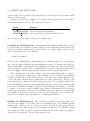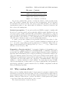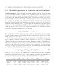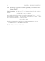
1
ADMB-RE
Random effects in AD Model Builder
A user guide
November 13, 2004
Contents
1 Introduction
1.1 Summary of features . . . . . . . . . . . . . . . . . . . . . . . . . . . . . .
3
3
2 The language and the program
2.1 What is ordinary ADMB? . . . . . . . . . . . . . . . . . . . . . .
2.2 Why random effects? . . . . . . . . . . . . . . . . . . . . . . . . .
2.2.1 A code example . . . . . . . . . . . . . . . . . . . . . . . .
2.2.2 Parameter estimation . . . . . . . . . . . . . . . . . . . . .
2.2.3 Log-normal random effects . . . . . . . . . . . . . . . . . .
2.3 Random effects modelling . . . . . . . . . . . . . . . . . . . . . .
2.3.1 Under the hood . . . . . . . . . . . . . . . . . . . . . . . .
2.3.2 Building a random effects model that works . . . . . . . .
2.4 Improving performance . . . . . . . . . . . . . . . . . . . . . . . .
2.4.1 Memory management; reducing the size of temporary files
2.4.2 Exploiting separability . . . . . . . . . . . . . . . . . . . .
2.4.3 Limited memory Newton optimization . . . . . . . . . . .
2.4.4 Gaussian priors and quadratic penalties . . . . . . . . . . .
2.4.5 Importance sampling . . . . . . . . . . . . . . . . . . . . .
2.4.6 Phases . . . . . . . . . . . . . . . . . . . . . . . . . . . . .
2.4.7 MCMC . . . . . . . . . . . . . . . . . . . . . . . . . . . .
2.5 Is ADMB a subset of ADMB-RE? . . . . . . . . . . . . . . . . . .
.
.
.
.
.
.
.
.
.
.
.
.
.
.
.
.
.
.
.
.
.
.
.
.
.
.
.
.
.
.
.
.
.
.
.
.
.
.
.
.
.
.
.
.
.
.
.
.
.
.
.
.
.
.
.
.
.
.
.
.
.
.
.
.
.
.
.
.
.
.
.
.
.
.
.
.
.
.
.
.
.
.
.
.
.
6
6
8
10
11
11
12
13
13
15
15
16
17
17
18
18
18
19
3 Example collection
3.1 Generalized additive models (GAM’s) . . . . . . . . . . . .
3.2 Nonparametric estimation of the variance function . . . . .
3.3 Mixed logistic regression; a comparison with WinBUGS . .
3.4 Discrete valued time series . . . . . . . . . . . . . . . . . .
3.5 Ordered categorical responses . . . . . . . . . . . . . . . .
3.6 Nonlinear mixed models; a comparison with NLME . . . .
3.7 Pharmacokinetics; a comparison with NLME . . . . . . . .
3.8 Weibull regression in censored survival analysis . . . . . .
3.9 Poisson regression with spatially correlated random effects
3.10 Stochastic volatility models for financial time series . . . .
.
.
.
.
.
.
.
.
.
.
.
.
.
.
.
.
.
.
.
.
.
.
.
.
.
.
.
.
.
.
.
.
.
.
.
.
.
.
.
.
.
.
.
.
.
.
.
.
.
.
20
21
24
26
27
28
29
30
31
32
33
A Command line options
.
.
.
.
.
.
.
.
.
.
.
.
.
.
.
.
.
.
.
.
.
.
.
.
.
.
.
.
.
.
.
.
.
.
.
.
.
.
.
.
34
2
Chapter 1
Introduction
This document is a user’s guide to random effects modelling in AD Model Builder (ADMB).
Chapter 2 is a concise introduction to ADMB, and chapter 3 is a collection of examples
selected from different fields of application. Online program code is provided for all examples. Supplementary documentation consists of
• The ADMB manual (http://otter-rsch.com/admodel.htm)
• Skaug & Fournier (2003), which describes the computational method (the Laplace
approximation) used to handle random effect in ADMB.
• The ADMB-RE example collection (http://otter-rsch.com/admbre/examples.html).
Why use AD Model Builder for creating nonlinear random effects models? The answer
consists of three words – flexibility, speed and accuracy. To illustrate these points a
number of examples comparing ADMB-RE with two existing packages NLME which runs
on R and Splus, and WinBUGS. In general NLME is rather fast and it is good for the
problems for which it was designed, but it is quite inflexible. What is needed is a tool
with at least the computational power of NLME but the flexibility to deal with arbitrary
nonlinear random effects models. In section 2.2.3 we consider a thread from the R user
list where a discussion about extending a model to use random effects which had a lognormal rather than normal distribution took place. This appeared to be quite difficult.
With ADMB-RE this change takes one line of code. WinBUGS on the other hand is very
flexible and many random effects models can be easily formulated in it. However, it can
be very slow and it is necessary to adopt a Bayesian perspective which may be a problem
for some applications. In section 3.3 we present a model which runs 25 times faster under
ADMB than under WinBUGS.
1.1
Summary of features
Model formulation With ADMB you can formulate and fit a large class of nonlinear
statistical models. With ADMB-RE you can include random effects in your model:
• Generalized linear mixed models (logistic and Poisson regression).
3
4
CHAPTER 1. INTRODUCTION
• Nonlinear mixed models (growth curve models, pharmacokinetics).
• State space models (nonlinear Kalman filter).
• Frailty models in survival analysis.
• Bayesian hierarchical models.
• General nonlinear random effects models (fisheries catch-at-age models).
You formulate the likelihood function in a template file, using a language that resembles
C++. The file is compiled into an executable program (Linux or Windows). The whole
C++ language is to your disposal, giving you great flexibility with respect to model
formulation.
Computational basis of ADMB-RE
• Hyper-parameters (variance components etc.) estimated by maximum likelihood.
• Marginal likelihood evaluated by the Laplace approximation or importance sampling.
• Exact derivatives calculated using Automatic Differentiation.
• Sampling from the Bayesian posterior using MCMC (Metropolis-Hastings algorithm).
• Most features of ADMB (matrix arithmetic and standard errors, etc.) are available.
The strengths of ADMB-RE
• Flexibility: You can fit a large variety of models within a single framework.
• Convenience: Computational details are transparent. Your only responsibility is to
formulate the loglikelihood
• Computational efficiency: ADMB-RE is up to 50 times faster than WinBUGS.
• Robustness: With exact derivatives you can fit highly nonlinear models.
• Convergence diagnostic: The gradient of the likelihood function provides a clear
convergence diagnostic.
Program interface
• Model formulation: You fill in a C++ based template using your favorite text editor.
• Compilation: You turn your model into an executable program using a C++ compiler (which you need to install separately).
• Platforms: Windows and Linux
1.1. SUMMARY OF FEATURES
5
How to order ADMB-RE ADMB-RE is a module for ADMB. Both can be ordered
from:
Otter Research Ltd
PO Box 2040,
Sidney, B.C. V8L 3S3
Canada
Voice or Fax (250)-655-3364
Email [email protected]
Internet: otter-rsch.com
Chapter 2
The language and the program
2.1
What is ordinary ADMB?
ADMB is a software package for doing parameter estimation in nonlinear models. It combines a flexible mathematical modelling language (built on C++) with a powerful function
minimizer (based on Automatic Differentiation). The following features of ADMB make
it very useful for building and fitting nonlinear models to data:
• Vector-matrix arithmetic, vectorized operations for common mathematical functions.
• Read and write vector and matrix objects to file.
• Fit the model is a stepwise manner (with ‘phases’), where more and more parameters
become active in the minimization.
• Calculate standard deviations of arbitrary functions of the model parameters by the
‘delta method’.
• MCMC sampling from Bayesian posteriors.
To use random effects in ADMB it is recommended that you have some experience in
writing ordinary ADMB programs. In this sections we review, for the benefit of the
reader without this experience, the basic constructs of ADMB needed for understanding
the examples presented in this manual.
Writing an ADMB program To fit a statistical model to data we must carry out
certain fundamental tasks, such as reading data from file, declaring the set of parameters
that should be estimated, and we must give a mathematical description of the model.
In ADMB you do all of this by filling in a template, which is an ordinary text file with
the file-name extension ‘.tpl’ (and hence the template file is known as the tpl-file). You
therefore need a text editor, such as ’vi’ under Linux or ’Notepad’ under Windows, to
write the tpl-file. The first tpl-file to which the reader of the ordinary ADMB manual is
exposed is simple.tpl (listed in Section 2.2.1 below). We shall use simple.tpl as our
6
2.1. WHAT IS ORDINARY ADMB?
7
generic tpl-file, and we shall see that introduction of random effects only requires small
changes to the program.
A tpl-file is divided into a number of ‘sections’, each representing one of the fundamental tasks mentioned above. The required sections are:
Name
DATA SECTION
PARAMETER SECTION
PROCEDURE SECTION
Purpose
Declare ‘global’ data objects; initialization from file
Declare independent parameters
Specify model and objective function in C++
More details are given when we later look at simple.tpl.
Compiling an ADMB program After having finished writing simple.tpl, we want
to convert it into an executable program. This is done in a DOS-window under Windows,
and in an ordinary terminal window under Linux. To compile simple.tpl, we would
under both platforms give the command:
$ admb -re simple
Here, ’$’ is the command line prompt (which may be a different symbol on your computer),
and -re is an option telling the program admb that your model contains random effects.
The program admb accepts another option -s which produces the ‘safe’ (but slower) version
of the executable program. The -s option should be used in a debugging phase, but it
should be skipped when the final production version of the program is generated.
The compilation process really consists of two steps: first simple.tpl is converted
to a C++ program by a preprosessor called tpl2rem. An error message from tpl2rem
consists of a single line of text, with a reference to the line in the tpl-file where the error
occurs. The first compilation step results in the C++ file simple.cpp. In the second
step simple.cpp is compiled and linked using an ordinary C++ compiler (which is not
part of ADMB). Error messages during this phase typically consist of long printouts, with
references to line numbers in simple.cpp. To track down syntax errors it may occasionally
be useful to look at the content of simple.cpp. When you understand what is wrong in
simple.cpp you should go back and correct simple.tpl and re-enter the command admb
-re simple. When all errors have been removed, the result will be an executable file,
which is called simple.exe under Windows or simple under Linux.
Running an ADMB-program The executable program is run in the same window as it was compiled. Note that ‘data’ are not usually part of the ADMB program
(simple.tpl). Instead, data are being read from a file with the file name extension
‘.dat’ (simple.dat). This brings us to the naming convention used by ADMB for input
and output files: The executable program automatically infers file names by adding an
extension to its own name. The most important files are:
8
CHAPTER 2. THE LANGUAGE AND THE PROGRAM
File name
Input
simple.dat
simple.pin
Output simple.par
simple.std
simple.cor
Contents
Data for the analysis
Initial parameter values
Parameter estimates
Standard deviations
Parameter correlations
You can use command line options to modify the behavior of the program at runtime. The available command line options are listed in Appendix 1, and are discussed
in detail under the various sections. An option you probably will like to use during an
experimentation phase is -est, which turns off calculation of standard deviations, and
hence reduces the running time.
Statistical prerequisites To use random effects in ADMB you must be familiar with
the notion of a random variable, and in particular with the normal distribution. In case
you are not, please consult a standard textbook in statistics. The notation u ∼ N (µ, σ 2 )
is used throughout this manual, and means that u has a normal (Gaussian) distribution
with expectation µ and variance σ 2 . The distribution placed on the random effects is
called the ’prior’, which is a term borrowed from Bayesian statistics.
A central concept that originates from generalized linear models is that of a linear predictor. Let x1 , . . . , xp denote observed covariates (explanatory variables), and let
β1 , . . . , βp be the corresponding regression parameters to be estimated. Many of the examples in this manual involve a linear predictor ηi = β1 x1,i + · · · + βp xp,i , which we also
will write on vector form η = Xβ.
Frequentist or Bayesian statistics? A pragmatic definition of a frequentist is a person who prefers to estimate parameters by maximum likelihood. Similarly, a Bayesian is
a person who use MCMC techniques to generate samples from the posterior distribution
(typically with noninformative priors on hyper-parameters), and from these samples generates some summary statistic such as the posterior mean. With its -mcmc runtime option
ADMB lets you switch freely between the two philosophies. Moreover, the approaches
complement each other rather than being competitors. A maximum likelihood fit (point
estimate + covariance matrix) is a step-1 analysis. For some purposes step-1 is sufficient. In other situations, one may want to see posterior distributions for the parameters,
and then the established covariance matrix is used by ADMB to implement an efficient
Metropolis-Hastings algorithm.
2.2
Why random effects?
Many people are familiar with the method of least squares for parameter estimation. Far
fewer know about random effects modeling. The use of random effects requires that we
adopt a statistical point of view, where the sum of squares is interpreted as being part of a
likelihood function. When data are correlated, the method of least squares is sub-optimal,
or even biased. But relax, random effects come to rescue!
The classical motivation of random effects is:
2.2. WHY RANDOM EFFECTS?
9
• To create parsimonious and interpretable correlation structures.
• To account for additional variation or overdispersion.
We shall see, however, that random effects are useful in a much wider context. For
instance, the problem of testing the assumption of linearity in ordinary regression (Example 3.1) is naturally formulated within ADMB-RE.
We use the simple.tpl example from the ordinary ADMB manual to exemplify the
use of random effects. The statistical model underlying this example is the simple linear
regression
Yi = axi + b + εi ,
i = 1, . . . , n,
where Yi and xi are the data, a and b are the unknown parameters to be estimated, and
εi ∼ N (0, σ 2 ) is an error term.
Consider now the situation that we do not observe xi directly, but rather we observe
Xi = xi + ei ,
where ei is a measurement error term. This situation frequently occurs in observational
studies, and is known as the ‘error in variables’ problem. Assume further that ei ∼
N (0, σe2 ), where σe2 is the measurement error variance. For reasons discussed below, we
must know the values of σe , so we shall pretend that σe = 0.5.
Because xi is not observed, we model it as a random effect with xi ∼ N (µ, σx2 ). In
ADMB-RE you are allowed to make such definitions through the new parameter type
random effects vector. (There is also a random effects matrix which allows you to
define a matrix of random effects).
1. Why do we call xi a random effect, while we do not use this term for Xi and
Yi (though they clearly are ’random’)? The point is that Xi and Yi are observed
directly, while xi is not. The term ’random effect’ comes from regression analysis,
where it means a random regression coefficient. In a more general context ’latent
random variable’ is probably a better term.
2. The unknown parameters in our model are: a, b, µ, σ, σx and x1 , . . . , xn . We have
agreed to call x1 , . . . , xn random effects. The rest of the parameters are called hyperparameters. Note that we place no prior distribution on the hyper-parameters.
3. Random effects are integrated out of the likelihood, while hyper-parameters are
estimated by maximum likelihood . This approach is often called ‘empirical Bayes’,
and will be considered a frequentist method by most people. There is however
nothing preventing you from making it ‘more bayesian’ by putting priors (penalties)
on the hyper-parameters.
4. A statistician will say ”this model is nothing but a bivariate Gaussian distribution
for (X, Y ), and we don’t need any random effects in this situation”. This is formally
true. We could work out the covariance matrix of (X, Y ) by hand and fit the
model using ordinary ADMB. This program would probably run much faster on
the computer, but it would have taken us longer time to write the code without
10
CHAPTER 2. THE LANGUAGE AND THE PROGRAM
declaring xi to be of type random effects vector. But, more important is that
random effects can be used also in non-Gaussian (nonlinear) models where we are
unable to derive an analytical expression for the distribution of (X, Y ).
5. Why didn’t we try to estimate σe ? Well, let us count the parameters in the model:
a, b, µ, σ, σx and σe ; totally six parameters. We know that the bivariate Gaussian
distribution has only five parameters (two means and three free parameters in the
covariate matrix). Thus, our model is not identifiable if we also try to estimate
σe . Instead, we pretend that we have estimated σe from some external data source.
This, example illustrates a general point in random effects modelling: you must be
careful to make sure that the model is identifiable!
2.2.1
A code example
Here is the random effects version of simple.tpl:
DATA_SECTION
init_int nobs
init_vector Y(1,nobs)
init_vector X(1,nobs)
PARAMETER_SECTION
init_number a
init_number b
init_number mu
vector pred_Y(1,nobs)
init_bounded_number sigma_Y(0.000001,10)
init_bounded_number sigma_x(0.000001,10)
random_effects_vector x(1,nobs)
objective_function_value f
PROCEDURE_SECTION
f = 0;
pred_Y=a*x+b;
// This section is pure C++
// Vectorized operations
// Prior part for random effects x
f += -nobs*log(sigma_x) - 0.5*norm2((x-mu)/sigma_x);
// Likelihood part
f += -nobs*log(sigma_Y) - 0.5*norm2((pred_Y-Y)/sigma_Y);
f += -0.5*norm2((X-x)/0.5);
f *= -1;
// ADMB does minimization!
2.2. WHY RANDOM EFFECTS?
11
Guide for the tpl-illiterate
1. Everything following ’//’ is a comment.
2. In the DATA SECTION, variables with a init in front of the data type are read from
file.
3. In the PARAMETER SECTION, variables with a init in front of the data type are the
hyper-parameters, i.e. the parameters to be estimated by maximum likelihood.
4. Variables defined in the PARAMETER SECTION without the init prefix can be used
as ordinary programming variables under the PROCEDURE SECTION. For instance, we
can assign a value to the vector pred Y.
5. ADMB does minimization, rather than optimization. Thus, the sign of the loglikelihood function f is changed in the last line of the code.
2.2.2
Parameter estimation
We learned above that hyper-parameters are estimated but maximum likelihood, but what
if we also are interested in the value of the random effects? For this purpose ADMB-RE
offers an ‘empirical Bayes’ approach, which involves fixing the hyper-parameters at their
maximum likelihood estimates, and treating the random effects as the parameters of the
model. ADMB-RE automatically calculates ‘maximum posterior’ estimates of the random
effects for you. Estimates of both hyper-parameters and random effects are written to
simple.par.
2.2.3
Log-normal random effects
Say that you doubt the distributional assumption xi ∼ N (µ, σx2 ) that was made in
simple.tpl, and that you want to check if a skewed distribution gives a better fit. You
could for instance take
xi = µ + σx exp(zi ),
zi ∼ N (0, 1).
Under this model the standard deviation of xi is proportional, but not directly equal, to
σx . It is easy to make this modification in simple.tpl. In the PARAMETER SECTION we
replace the declaration of x by
vector x(1,nobs)
random_effects_vector z(1,nobs)
and in the PROCEDURE SECTION we replace the prior on x by
f = - 0.5*norm2(z);
x = mu + sigma_x*exp(z);
12
CHAPTER 2. THE LANGUAGE AND THE PROGRAM
This example shows one of the strengths of ADMB-RE: it is very easy to modify
models. In principle you can implement any random effects model you can think of, but
as we shall discuss later, there are limits to the number of random effects you can declare.
2.3
Random effects modelling
Random effects were motivated in the previous section. Now, we teach you how to write
your own programs. The objective function in random effects models has two parts:
1. The prior, which is the log-probability density of the random effects.
2. The likelihood, which is the log-probability density of data, specified in terms of the
random effects and hyper-parameters.
ADMB does not impose this structure on the tpl-file, but organizing the code in this
way improves readability.
F The order in which the different loglikelihood contributions are added to the objective function does not matter, but make sure that all programming variables have
got their value assigned before they enter in a prior or a likelihood expression.
In simple.tpl we declared x1 , . . . , xn to be of type random effects vector. This
statement tells ADMB that x1 , . . . , xn should be treated as random effects (i.e. be the
targets for the Laplace approximation), but it does not say anything about which distribution the random effects should have. In the simple.tpl we assumed that xi ∼ N (µ, σx2 ),
and (without saying it explicitly) that the xi ’s were statistically independent. We know
that the corresponding prior contribution to the loglikelihood is
−n log(σx ) −
1 X
(xi − µ)2 .
2σx2 i=1
The corresponding ADMB code is
f += -nobs*log(sigma_x) - 0.5*norm2((x-mu)/sigma_x);
Usually, the random effects will have a Gaussian distribution, but in theory there is
nothing preventing you from replacing the above line by for instance a log-gamma density
(although the Laplace approximation may then not perform as well).
A frequent source of error when writing ADMB-RE programs is that prior gets wrongly
specified. The following trick can make the code easier to read, and has the additional
advantage of being numerically stable for small values of σx . From basic probability theory
we know that if u ∼ N (0, 1), then x = σx u + µ will have a N (µ, σx2 ) distribution. The
corresponding ADMB code would be
2.3. RANDOM EFFECTS MODELLING
13
f += - 0.5*norm2(u);
x = sigma_x*u + mu;
(This, of course, requires that we change the type of x from random effects vector to
vector, and that u is declared as a random effects vector.) So, the trick here was to
start with N (0, 1) distributed random effects, and to build the model from them. This is
however not allways the preferred strategy, as we shall see later.
Similarly, the likelihood contribution coming from data (Xi and Yi in simple.tpl)
must be added to the objective function. Typically, you will use the binomial, Poisson,
gamma or Gaussian distribution for your data, but you are not restricted to these distributions. There are no built-in probability distributions, so you will have to write the
mathematical expressions yourself, as we did for the Gaussian distribution above.
2.3.1
Under the hood
The random effects are important building blocks in simple.tpl, but how are they treated
internally in ADMB-RE? Since the random effects are not observed data they have parameter status, but we distinguish them from the hyper-parameters. This is because the
xi are random variables. In the marginal likelihood function used internally by ADMBRE to estimate hyper-parameters, the random effects are ‘integrated out’. The purpose
of the integration is to generate the marginal probability distribution for the observed
quantities, which are X and Y in simple.tpl. In that example we could have found an
analytical expression for the marginal distribution of (X, Y ), because only normal distributions were involved. For other distributions, such as the binomial, no simple expression
for the marginal distribution exists, and hence we must rely on ADMB to do the integration. In fact, the core of what ADMB-RE does for you is that it automatically calculates
the marginal likelihood, at the same time as it estimates the hyper-parameters. The integration technique used by ADMB-RE is the so-called Laplace approximation (Skaug &
Fournier 2003).
The algorithm used internally by ADMB-RE to estimate hyper-parameters involves
iterating between the two steps:
1. The ‘penalized likelihood’ step: Maximizing the likelihood with respect to the random effects, while holding the value of the hyper-parameters fixed.
2. Updating the value of the hyper-parameters, using the estimates of the random
effects obtained in 1).
The reason for calling the objective function in 1) a penalized likelihood, is that the prior
on the random effects acts as a penalty function.
2.3.2
Building a random effects model that works
In all nonlinear parameter estimation problems, there are two possible explanations when
your program does not produce meaningful results:
14
CHAPTER 2. THE LANGUAGE AND THE PROGRAM
1. The underlying mathematical model is not well defined, e.g. it may be over-parameterized.
2. You have implemented the model incorrectly, e.g. you have forgotten a ‘minus’ sign.
In an early phase of the code development it may not be clear which of these is causing the
problem. With random effects, the two-step iteration scheme described above makes it
even more difficult to find the error. We therefore advise you always to check the program
on simulated data, for which the true parameter values are known, before you apply it to
your real dataset. This section gives you a recipe for how to do this.
The first thing you should do after having finished the tpl-file is to check that the
penalized likelihood step is working correctly. In ADMB it is very easy to switch from a
random effects version of the program to a penalized likelihood version. In simple.tpl
we would simply redefine the random effects vector x to be of type init vector. The
parameters would then be a, b, µ, σ, σx and x1 , . . . , xn . It is not recommended, or even
possible, to estimate all of these simultaneously, so you should fix σx (by giving it a phase
‘-1’) at some reasonable value. The actual value at which you fix σx is not critically
important, and you could even try a range of σx values. In larger models there will be
more than one parameter that needs to be fixed.
In summary, the following steps will ensure the correctness of you tpl-file:
1. Write a simulation program (in R, S-Plus, Matlab, or some other program) that
generates data from the random effects model (using some reasonable values for the
parameters) and writes to simple.dat.
2. Fit the penalized likelihood program with σx (or the equivalent parameters) fixed
at the value used to simulate data.
3. Compare the estimated parameters with the parameter values used to simulate data.
In particular, you should plot the estimated random effects against the simulated
random effects. The plotted points should centre around a straight line. If they do
(to some degree of approximation) you most likely have got a correct formulation
of the penalized likelihood.
If your program passes this test, you are ready to test the random effects version of the
program. You redefine x to be of type random effects vector, free up σx , and apply
again your program to the same simulated dataset. If the program produces meaningful
estimates of the hyper-parameters, you most likely have got a correct program, and you
are ready to move on to your real data!
With random effects it often happens that the maximum likelihood estimate of the
variance components is zero (σx = 0). Parameters bouncing against the boundaries
usually makes one feel uncomfortable, but with random effects the interpretation of σx = 0
is clear and unproblematic. All it really means is that data do not support a random
effect, and the natural consequence is to remove (or inactivate) x1 , . . . , xn , together with
the corresponding prior (and hence σx ), from the model.
2.4. IMPROVING PERFORMANCE
2.4
15
Improving performance
In this section we discuss certain mechanisms you can use to make an ADMB-RE program
run faster, or to produce more accurate estimates.
2.4.1
Memory management; reducing the size of temporary files
When ADMB needs more temporary storage than is available in the allocated memory
buffers, it starts producing temporary files. Since writing to disk is much slower than
accessing memory, it is important to reduce the size of temporary files as much as possible.
There are several parameters (such as arrmblsize) built into ADMB that regulates how
large memory buffers an ADMB program allocates at startup. With random effects the
memory requirements increases dramatically, and ADMB deals with this by producing
(when needed) six temporary files:
File name
f1b2list1
f1b2list12
f1b2list13
nf1b2list1
nf1b2list12
nf1b2list13
Command line option
-l1 N
-l2 N
-l3 N
-nl1 N
-nl2 N
-nl3 N
The table also shows the command line arguments you can use to manually set the size
(determined by N) of the different memory buffers.
When you see any of these files start growing, you should kill your application and
restart it with the appropriate command line options. In addition to the options shown
above there is -ndb N that splits the computations into N chunks. This effectively reduces
the memory requirements by a factor of N , at the cost of a somewhat longer run time.
The -ndb option can be used in combination with the -l and -nl options listed above.
The following rule-of-thumb for setting N in -ndb N can be used: if there are totally m
random effects in the model, one should choose N such that m/N ≈ 50. For most of the
models in the example collection (Chapter 3) this choice of N prevents any temporary
files of being created.
Consider the model in Section 3.1 as an example. This model contains only about
60 random effects, but does rather heavy computations with these, and as a consequence
large temporary files are generated. The following command line
$ ./union -l1 10000000 -l2 100000000 -l3 10000000 -nl1 10000000
takes away the temporary files but requires 80Mb of memory. The command line
$ ./union -est -ndb 5 -l1 10000000
also runs without temporary files, requires only 20Mb of memory, but runs three times
slower.
Finally, a warning about the use of these command line options. If you allocate
too much memory your application will die without any meaningful error message. So,
16
CHAPTER 2. THE LANGUAGE AND THE PROGRAM
you should monitor the memory use of your application using “Task Manager” under
Windows and the command “top” under Linux, to ensure that you do not exceed the
available memory on your computer.
2.4.2
Exploiting separability
In practice, there is an upper limit to the number q of random effects you can include
in your model. The reason is that the computational cost of performing the Laplace approximation goes as O(q 3 ). Roughly speaking, the upper bound is q = 500, although this
number depends strongly on the particular model. In many cases, such as with time series
models, the problem has a special structure that can be exploited to reduce the computational complexity. In statistics this structure is called ‘conditional independence’, while in
the optimization literature it is called ‘partial separability’. When the objective function
is (partial) separable, models with several thousand random effects can be handled in
ADMB-RE.
Partial separability is the property that the objective function g can be written as a
sum of terms that each only depends on a small number of random effects. The simplest
example is a one-way variance component model
yij = µ + ui + εij ,
i = 1, . . . , q,
j = 1, . . . , ni
where ui ∼ N (0, σu2 ) is a random effect and εij ∼ N (0, σ 2 ) is an error term. In the
straightforward implementation of this model we declare
random_effects_vector u(1,q)
and compute the objective function as
for(i=1;i<=q;i++)
{
g += -log(sigma_u) - 0.5*square(u(i)/sigma_u);
for(j=1;j<=n(i);j++)
g += -log(sigma) - 0.5*square((y(i,j)-mu-u(i))/sigma);
}
The ‘sum’ referred to above is represented by the outer for-loop. We need to tell ADMB
explicitly what the separability structure is. We do this in the tpl-file by placing the
code between { and } in a user defined sub-routine which we here call g cluster. Our
PROCEDURE SECTION then would consist of
for(i=1;i<=q;i++)
g_cluster(i,u(i),mu,sigma,sigma_u);
Objects defined in the DATA SECTION are ‘global’ and do not need to be passed as arguments to g cluster. Similarly, the objective function g is a global object. We place
the code g cluster in a code-section called SEPARABLE FUNCTION. Examples 3.7 and 3.4
show the details about how to do this.
2.4. IMPROVING PERFORMANCE
17
Why is separability important? When evaluating the Laplace approximation ADMB
calculates a matrix of second order partial derivatives of the objective function g with
respect to the random effects. When g is separable most of the elements in this matrix
are zero, and ADMB can avoid calculating these elements. The two main categories of
separable models are:
• Nested models in regression with categorical covariates, of which the one-way variance component model is the simplest example.
• State space models (time series models), in which the equivalent of g cluster would
depend on u(i-1) and u(i), say.
2.4.3
Limited memory Newton optimization
The penalized likelihood step (Section 2.3.1), that forms a crucial part of the algorithm
used by ADMB to estimate hyper-parameters, is by default conducted using a quasiNewton optimization algorithm. If the number of random effects is large, as it typically
is for separable models, it may be more efficient to use a ‘limited memory quasi-Newton’
optimization algorithm. This is done using the command line argument -ilmn N, where N
is the number of steps to keep. Typically N=5 is a good choice. An example that benefits
from the use of -ilmn is given in Example 3.10.
2.4.4
Gaussian priors and quadratic penalties
In most models the prior for the random effect will be Gaussian. In some situations,
such as in spatial statistics, the random effects will be correlated. ADMB contains a
special feature (the normal prior keyword) for dealing efficiently with such models. The
construct used to declaring a correlated Gaussian prior is
random_effects_vector u(1,n)
normal_prior S(u);
The first of these lines is an ordinary declaration of a random effects vector. The second
line tells ADMB that u has a multivariate Gaussian distribution with zero expectation
and covariance matrix S , i.e. the probability density of u is
1 0 −1
−1/2
−1/2
h(u) = (2π)
det(S)
exp − u S u .
2
Here, S is allowed to depend on the hyper-parameters of the model. The part of the code
where S gets assigned its value must be placed in a SEPARABLE FUNCTION (see Example
3.9).
F The log-prior log (h (u)) is automatically subtracted from the objective function. It
is thus necessary that the objective function holds the negative loglikelihood when
using the normal prior.
18
CHAPTER 2. THE LANGUAGE AND THE PROGRAM
F To verify that your model really is partially separable you should try replacing the
SEPARABLE FUNCTION keyword with an ordinary FUNCTION. Then verify on a small
subset of your data that the two versions of the program produce the same results.
You should be able to observe that the SEPARABLE FUNCTION-version runs faster.
2.4.5
Importance sampling
The Laplace approximation may be inaccurate in some situations . The quality of the
approximation may then be improved by adding an importance sampling step. This is
done in ADMB by using the command line argument -is N, where N is the sample size in
the importance sampling. Increasing N will give better accuracy, at the price of a longer
run time. As a rule-of-thumb you should start with N=100, and increase N stepwise by a
factor of 2 until the parameter estimates stabilize.
2.4.6
Phases
A very useful feature of ADMB is that it allows the model to be fit in different phases.
In the first phase you estimate only a subset of the parameters, with the remaining
parameters being fixed at their initial values. In the second phase more parameters are
turned on, and so on. The phase in which a parameter becomes active is specified in the
declaration of the parameter. By default, a parameter has phase 1. A simple example
would be
PARAMETER_SECTION
init_number a(1)
init_number b(2)
where a becomes active in phase 1, while b becomes active in phase 2. With random
effects we have the following rule-of-thumb for the use of phases:
1. Activate the random effects and the corresponding variance parameter in phase 2.
2. Activate the remaining hyper-parameters in phase 1.
When there is more than one random effects vector, it may be advantageous to let these
become active in different phases (see Example 3.2).
2.4.7
MCMC
From a user perspective the -mcmc option works exactly the same way as with ordinary
ADMB. However, under the hood, there is one important difference. The MetropolisHastings algorithm is applied only to the hyper-parameters, while the random effects are
being integrated out by the Laplace approximation. This speeds up the mixing of the
Markov chain, and makes it much easier to judge convergence, because you typically will
have a small number of hyper-parameters.
2.5. IS ADMB A SUBSET OF ADMB-RE?
2.5
19
Is ADMB a subset of ADMB-RE?
You will find that not all the functionality of ordinary ADMB has yet been implemented
in ADMB-RE. Functions are being added all the time. The following functions have been
implemented:
• Arithmetic operators for scalars, vectors and matrices.
• The exponential function exp.
Chapter 3
Example collection
The examples in this section serve two purposes: they show the breadth of the class of
models that can be fitted with ADMB-RE, and they can be used as templates for new
models. The examples may be categorized as follows:
Plain ADMB-RE
Separability
Gaussian prior
Regression Survival ana. Time series
3.2, 3.1, 3.3
3.8
3.8, 3.6, 3.7
3.4, 3.10
Spatial statistics
3.9
Program files (tpl, dat, and par-files) for all examples can be obtained from:
http://otter-rsch.com/admbre/examples.html
20
3.1. GENERALIZED ADDITIVE MODELS (GAM’S)
3.1
21
Generalized additive models (GAM’s)
Model description A very useful generalization of the ordinary multiple regression
yi = µ + β1 x1,i + · · · + βp xp,i + εi ,
is the class of additive models,
yi = µ + f1 (x1,i ) + · · · + fp (xp,i ) + εi .
(3.1)
Here, the fj are ‘nonparametric’ components which can be modelled by penalized splines.
When this generalization is carried over to generalized linear models, and we arrive at the
class of GAM’s (Hastie & Tibshirani 1990). From a computational perspective penalized
splines are equivalent to random effects, and thus GAM’s fall naturally into the domain
of ADMB-RE.
For each component fj in (3.1) we construct a design matrix X such that fj (xi,j ) =
(i)
X u, where X(i) is the ith row of X and u is a coefficient vector. We use the R-function
splineDesign (from the splines library) to construct a design matrix X. To avoid
overfitting we add a first order difference penalty (Eilers & Marx 1996):
X
− λ2
(uk − uk−1 )2 ,
(3.2)
k=2
to the ordinary GLM loglikelihood, where λ is a smoothing parameter to be estimated.
By viewing u as a random effects vector with the above Gaussian prior, and by taking λ
as a hyper-parameter, it becomes clear that GAM’s are naturally handled in ADMB-RE.
Implementation details
• A computationally more efficient implementation is obtained by moving λ from the
penalty term to the design matrix, i.e. fj (xi,j ) = λ−1 X(i) u.
P
• Since (3.2) does not penalize the mean of u, we impose the restriction that k=1 uk =
0 (see the union.tpl for details). Without this restriction the model would be overparameterized since we already have an overall mean µ in (3.1).
• To speed up computations the parameter µ (and other regression parameters) should
be given ‘phase 1’ in ADMB, while the λ’s and the u’s should be given ‘phase 2’.
The Wage-union data The data, which are available from Statlib (lib.stat.cmu.edu/),
contain information for each of 534 workers about whether they are members (yi = 1) of
a workers union or not (yi = 0). We study the probability of membership as a function of
six covariates. Expressed in the notation used by the R (S-Plus) function gam the model
is:
union ~race + sex + south + s(wage) + s(age) + s(ed), family=binomial
Here, s() denotes a spline functions with 20 knots each. For wage a cubic spline is used,
while for age and ed quadratic splines are used. The total number of random effects
that arise from the three corresponding u vectors is 64. Figure 3.1 shows the estimated
nonparametric components of the model. The time taken to fit the model was 165 seconds.
22
CHAPTER 3. EXAMPLE COLLECTION
Figure 3.1: Union data: Probability of membership as a function of covariates. In each
plot, the remaining covariates are fixed at their sample means. The effective degrees of
freedom (df) are also given (Hastie & Tibshirani 1990).
3.1. GENERALIZED ADDITIVE MODELS (GAM’S)
23
Extensions
• The linear predictor may be a mix of ordinary regression terms (fj (x) = βj x) and
nonparametric terms. ADMB-RE offers a unified approach to fitting such models, in
which the smoothing parameters λj and the regression parameters βj are estimated
simultaneously.
• It is straightforward in ADMB-RE to add ‘ordinary’ random effects to the model,
for instance to accommodate for correlation within groups of observations, as in Lin
& Zhang (1999).
24
CHAPTER 3. EXAMPLE COLLECTION
3.2
Nonparametric estimation of the variance function
Model description An assumption underlying the ordinary regression
yi = a + bxi + ε0i
is that all observations have the same variance, i.e. Var(ε0i ) = σ 2 . This assumption does
not always hold, e.g. in Figure 3.2 a). It is clear that the variance increases to the right
(for large values of x). It is also clear that the mean of y is not a linear function of x. We
thus fit the model
yi = f (xi ) + σ(xi )εi ,
where εi ∼ N (0, 1), and f (x) and σ(x) are modelled nonparametrically. As in Example 3.1
we take f to be a penalized spline. To ensure that σ(x) > 0 we model log [σ(x)] , rather
than σ(x), as a spline function. For f we use a cubic spline (20 knots) with a 2nd order
difference penalty
−λ
2
20
X
(uj − 2uj−1 + uj−2 )2 ,
k=3
while we take log [σ(x)] to be a linear spline (20 knots) with the 1st order difference
penalty (3.2).
Implementation details Details on how to implement spline components are given
Example 3.1.
• In order to estimate the variation function, one first needs to have fitted the mean
part. Parameter associated with f should thus be given ‘phase 1’ in ADMB, while
those associated with σ should be given ‘phase 2’.
3.2. NONPARAMETRIC ESTIMATION OF THE VARIANCE FUNCTION
25
−0.4
−0.8
y
0.0
LIDAR data
400
450
500
550
600
650
700
650
700
x
0.05
0.00
SD
0.10
0.15
Standard derviation
400
450
500
550
600
x
Figure 3.2: LIDAR data (upper panel) used by Ruppert et al. (2003) with fitted mean.
Fitted standard deviation is shown in the lower panel.
26
3.3
CHAPTER 3. EXAMPLE COLLECTION
Mixed logistic regression; a comparison with WinBUGS
Model description Let y = (y1 , . . . , yn ) be a vector of dichotomous observations (yi ∈
{0, 1}), and let u = (u1 , . . . , uq ) be a vector of independent random effects, with ui ∼
N (0, σ 2 ). The following relationship between the success probability πi = Pr(yi = 1) and
explanatory variables (contained in matrices X and Z) is assumed:
πi
log
= Xi β + Zi u,
1 − πi
where Xi and Zi are the i’th rows of the known design matrices X and Z , respectively,
and β is a vector of regression parameters. Thus, the hyper-parameters of the model are
β and σ.
Results Our goal is to compare computation times with WinBUGS on a simulated
data set. For this purpose we use n = 200, p = 5, q = 30, σ = 0.1 and βj = 0 for all
j. The covariate matrices X and Z are generated randomly with each element uniformly
distributed on [−2, 2] . As start values for both ADMB and WinBUGS we use βj = −1
and σ = 4.5. In WinBUGS we use a uniform [−10, 10] prior for βj and a standard (in the
WinBUGS literature) noninformative gamma prior on τ = σ −2 . In ADMB the parameter
constraints βj ∈ [−10, 10] and log(σ) ∈ [−5, 3] are used in the optimization process.
On the simulated dataset ADMB used 15 seconds to converge to the optimum of
likelihood surface. On the same dataset we first ran WinBUGS (Version 1.4) for 5, 000
iterations. The recommended convergence diagnostic in WinBUGS is the Gelman-Rubin
plot (see the help files available from the menus in WinBUGS), which requires that at
least two Markov chains are run in parallel. From the Gelman-Rubin plots for σ and β it
was apparent that convergence occurred after approximately 2, 000 iterations. A few of
the components of u did not yet seem to have reached equilibrium. The time taken by
WinBUGS to perform 2, 000 iterations of two chains was approximately 700 seconds. The
estimate of σ was 0.1692 as calculated by AD Model Builder, while the posterior mean
estimate calculated by WinBUGS σ was 0.1862.
The robustness of the two approaches was investigated by decreasing the amount
of information while holding the number of parameters (p and q) constant. For n =
50, WinBUGS came up with an error message before convergence was reached. ADMB
converged without problems to the optimum of the likelihood function, although observed
Fisher information matrix showed that the hyper-parameters were weakly determined.
3.4. DISCRETE VALUED TIME SERIES
3.4
27
Discrete valued time series
Model description Most of the time series literature is concerned with continuous
outcome. To construct models for time-correlated counts, one can use a ‘state-space’
approach . A state-space model has two components:
1. The ‘state equation’, which we implement using random effects.
2. The ‘observation equation’, which we take as the Poisson likelihood.
The state equation specifies that the state variable ui follow a latent autoregressive process
ei ∼ N (0, σ 2 ).
ui = aui−1 + ei ,
There are two candidates for being our random effects: ui and ei .
F If we take ui to be the random effects, the model becomes separable.
If we instead choose ei , the model does not become separable, because ui depends on all
of e1 , . . . , ei .) The ADMB-RE code for the separable model is
random_effects_vector u(1,n)
and
for (i=2;i<=n;i++)
g += -log(sigma) -.5*square((u(i)-a*u(i-1))/sigma);
To exploit the separability structure, we need to place the above code in a SEPARABLE FUNCTION
section. The ’observation equation’ for this model simply states that the observations yi
has a Poisson distribution with parameter λi = exp(ηi + ui ), where ηi is a linear predictor.
Results Zeger (1988) analyzed a time series of monthly numbers of poliomyelitis cases
during the period 1970-1983 in the US. We make comparison to the performance of the
Monte Carlo Newton-Raphson method of Kuk & Cheng (1999). Let yi denote the number
of polio cases in the i’th period. There are six covariates that account for trend and
seasonal effects.
Estimates of hyper-parameters are shown in the following table.
β1
ADMB-RE
0.242
Std. dev.
0.27
Kuk & Cheng (1999) 0.244
β2
-3.81
2.76
-3.82
β3
0.162
0.15
0.162
β4
-0.482
0.16
-0.478
β5
0.413
0.13
0.413
β6
-0.0109
0.13
-0.0109
a
0.627
0.19
0.665
σ
0.538
0.15
0.519
The standard deviation is large for several regression parameters. The ADMB-RE estimates (based on the Laplace approximation) are very similar to the exact maximum
likelihood estimates as obtained with the method of Kuk & Cheng (1999).
Kuk & Cheng (1999) reported that the computation time for their method was 3120
seconds. The run time for ADMB-RE was 66 seconds.
28
3.5
CHAPTER 3. EXAMPLE COLLECTION
Ordered categorical responses
Model description In the standard logistic regression there are S = 2 possible outcomes (success and failure). A generalization of this model is to allow outcomes to come
from the ordered set y (1) < y (2) < · · · < y (S) . The probability associated with y (s) is
denoted by πs , and is defined through:
s
X
j=1
πj =
exp(κs − η)
,
1 + exp(κs − η)
s = 1, . . . , S − 1,
where κ1 < · · · < κS−1 are parameters and η is a linear predictor depending on covariates.
The SOCATT data set is used in a software review conducted by the Centre for Multilevel Modelling (http://multilevel.ioe.ac.uk/softrev/index.html). The SOCATT data
consist of responses to a set of dichotomous items on a woman’s right to have an abortion under different circumstances. The outcome variable y is a score constructed from
these items ranging from 1 to 7, with a higher score corresponding to stronger support
for abortion. Each of q = 264 respondents was asked the same set of questions on four
occasions (hence n = 1056) in the period 1983 − 1986, and yij denotes the response for
individual i at year j. We consider three indicator variables (x1 , x2 , x3 ) and the following
linear predictor
ηi = β1 xij1 + β2 xij2 + β3 xij3 + ui ,
with ui ∼ N (0, σ 2 ).
Results Estimates of hyper-parameters are shown in the following table:
ADMB-RE
aML
β1
β2
β3
σ
κ1
1.953 0.684 2.775 2.229 -4.127
2.064 0.688 2.841 2.283 -4.056
κ2
κ3
κ4
κ5
κ6
-2.390 0.402 1.337 2.225 3.265
-2.300 0.510 1.449 2.341 3.384
The computation time (ADMB-RE) for this model was 30 seconds on a 1,400 MHz PC
running linux, while for the packages participating in the software review the computation
times ranged from 5 to 60 seconds.
3.6. NONLINEAR MIXED MODELS; A COMPARISON WITH NLME
3.6
29
Nonlinear mixed models; a comparison with NLME
Model description The orange tree growth data was used by Pinheiro & Bates (2000,
Ch.8.2) to illustrate how a logistic growth curve model with random effects can be fit
with the S-Plus function nlme. The data contain measurements made at seven occasions
for each of five orange trees:
tij
yij
Time point when the jth measurement was made on tree i
Trunk circumference of tree i when measured at time point tij
The following logistic model is used:
yij =
φ1 + ui
+ εij ,
1 + exp [− (tij − φ2 ) /φ3 ]
where (φ1 , φ2 , φ3 ) are hyper-parameters, and ui ∼ N (0, σu2 ) is a random effect, and εij ∼
N (0, σ 2 ) is the residual noise term.
Results Parameter estimates are shown in the following table.
ADMB-RE
Std. dev.
nlme
φ1
192.1
15.658
191.0
φ2
727.9
35.249
722.6
φ3
348.1
27.08
344.2
σ
7.843
1.013
7.846
σu
31.65
10.26
31.48
The difference between the estimates obtained with ADMB-RE and nlme is small.
The difference is caused by the fact that the two approaches use different approximations
to the likelihood function. (ADMB-RE uses the Laplace approximation, and for nlme the
reader is referred to (Pinheiro & Bates 2000, Ch. 7).)
The computation time for ADMB was 0.58 seconds, while the computation time for
nlme (running under S-Plus 6.1) was 1.6 seconds. Because NLME is design for this kind
of models, it can be expected that it will be faster than a general purpose package such
as ADMB, although the difference is not very large in this particular problem.
30
3.7
CHAPTER 3. EXAMPLE COLLECTION
Pharmacokinetics; a comparison with NLME
Model description The ‘one-compartment open model’ is commonly used in pharmacokinetics. It can be described as follows. A patient receives a dose D of some substance
at time td . The concentration ct at a later time point t is governed by the equation
D
Cl
ct = exp − (t − td )
V
V
where V and Cl are parameters (the so-called ‘Volume of concentration’ and the ‘Clearance’). Doses given at different time points contribute additively to ct . Pinheiro & Bates
(2000, Ch. 6.4) fitted this model to a dataset using the S-Plus routine nlme. The linear
predictor used by Pinheiro & Bates (2000, p. 300) is:
log (V ) = β1 + β2 W t + uV ,
log (Cl) = β3 + β4 W t + uCl ,
2
where W t is a continuous covariate, and uV ∼ N (0, σV2 ) and uCl ∼ N (0, σCl
) are random effects. The model specification is completed by the requirement that the observed
concentration y in the patient is related to the true concentration by y = ct + ε, where
ε ∼ N (0, σ 2 ) is a measurement error term.
Results Estimates of hyper-parameters are shown in the following table:
ADMB-RE
Std. Dev
nlme
β1
-5.99
0.13
-5.96
β2
0.622
0.076
0.620
β3
-0.471
0.067
-0.485
β4
0.532
0.040
0.532
σ
2.72
0.23
2.73
σV
0.171
0.024
0.173
σCl
0.227
0.054
0.216
The differences between the estimates obtained with ADMB-RE and nlme are caused
by the fact that the two methods use different approximations of the likelihood function.
ADMB-RE uses the Laplace approximation, while the method used by nlme is described
in Pinheiro & Bates (2000, Ch. 7).
The time taken to fit the model by ADMB-RE was 17 seconds, while the computation
time for nlme (under S-Plus 6.1) was 7 seconds. Because NLME is design for this kind of
models, it can be expected that it will be faster than a general purpose package such as
ADMB, although the difference is not very large in this problem.
3.8. WEIBULL REGRESSION IN CENSORED SURVIVAL ANALYSIS
3.8
31
Weibull regression in censored survival analysis
Model description A typical setting in survival analysis is that we observe the time
point t at which the death of a patient occurs. Patients may leave the study (for some
reason) before they die. In this case the survival time is said to be censored, and t refers
to the time point when the patient left the study. The indicator variable δ is used to
indicate whether t refers to the death of the patient (δ = 1) or to a censoring event
(δ = 0). The key quantity in modelling the probability distribution of t is the hazard
function h(t), which measures the instantaneous
death rate at time t. We also define the
Rt
cumulative hazard function H(t) = 0 h(s)ds, implicitly assuming that the study started
at time t = 0. The loglikelihood contribution from our patient is δ log(h(t)) − H(t). A
commonly used model for h(t) is Cox’s proportional hazard model, in which the hazard
rate for the ith patient is assumed to be on the form
hi (t) = h0 (t) exp(ηi ),
i = 1, . . . n.
Here, h0 (t) is the “baseline” hazard function (common to all patients) and ηi is a linear
predictor. In this example we shall assume that the baseline hazard belongs to the Weibull
family: h0 (t) = rtr−1 for r > 0.
In the collection of examples following the distribution of WinBUGS this model is
used to analyze a dataset on times to kidney infection for a set of n = 38 patients
(‘Kidney: Weibull regression with random effects’, Examples Volume 1, WinBUGS 1.4).
The dataset contains two observations per patient (the time to first and second recurrence
of infection). In addition there are three covariates: ‘age’ (continuous), ‘sex’ (dichotomous)
and ‘type of disease’ (categorical, four levels), and an individual specific random effect
ui ∼ N (0, σ 2 ). Thus, the linear predictor becomes
ηi = β0 + βsex · sexi + βage · agei + βD xi + ui ,
(3.3)
where βD = (β1 , β2 , β3 ) and xi is a dummy vector coding for the disease type. Parameter
estimates are shown in the table below. Posterior means as calculated by WinBUGS are
also shown in the table, and are similar to the maximum likelihood estimates.
ADMB-RE
Std. dev.
BUGS
Std. dev.
β0
-4.344
0.872
-4.6
0.8962
βage
0.003
0.0137
0.003
0.0148
β1
0.1208
0.5008
0.1329
0.5393
β2
0.6058
0.5011
0.6444
0.5301
β3
-1.1423
0.7729
-1.168
0.8335
βsex
-1.8767
0.4754
-1.938
0.4854
r
1.1624
0.1626
1.215
0.1623
σ
0.5617
0.297
0.6374
0.357
32
3.9
CHAPTER 3. EXAMPLE COLLECTION
Poisson regression with spatially correlated random effects
Model description Let {ξ(z), z ∈ R2 } be a Gaussian random field with correlation
structure
corr {ξ(z), ξ(z0 )} = exp −α−1 d(z, z0 ) ,
where d(z, z0 ) is the Euclidean distance between the points z and z0 . Let y1 , . . . , yn be observations made at locations z1 , . . . , zn , respectively. Conditionally on ξ = {ξ(z1 ), . . . , ξ(zn )}
the y’s are independent with yi ∼ Poisson(λi ), where
log (λi ) = Xi β + ξ(zi ).
Here, Xi β is a linear predictor, and the vector of hyper-parameters is θ = (β, σ, α).
We fit this model to n = 100 simulated data points.
Results It takes 3 minuts to fit the model.
3.10. STOCHASTIC VOLATILITY MODELS FOR FINANCIAL TIME SERIES
3.10
33
Stochastic volatility models for financial time
series
Model description Stochastic volatility models are used in mathematical finance to
describe the evolution of asset returns, which typically exhibit changing variances over
time. As an illustration we use a time series of daily pound/dollar exchange rates {zt }
from the period 01/10/81 to 28/6/85, previously analyzed by Harvey, Ruiz & Shephard
(1994). The series of interest are the daily mean-corrected returns {yt }, given by the
transformation
n
X
−1
yt = log zt − log zt−1 − n
(log zt − log zt−1 ) .
i=1
The stochastic volatility model allows the variance of yt to vary smoothly with time. This
is achieved by assuming that yt ∼ N (µ, σt2 ), where σt2 = exp (µx + xt ). The smoothly
varying component xt follows the autoregression
xt = βxt−1 + εt ,
εt ∼ N (0, σ 2 ).
The vector of hyper-parameters is for this model is thus (β, σ, µ, µx ).
Appendix A
Command line options
A list of command line options accepted by ADMB-applications can be obtained by giving
the option -? to the application, for instance simple -?. The following command line
options are specific to ADMB-RE, but are not listed by -?.
Option
Explanation
-is N
use importance sampling with sample size N
-nr N
performs N Newton-Raphson steps in the Laplace approximation
-imaxfn N performs N optimization steps in the Laplace approximation
-ilmn N
N-step limited memory quasi Newton for random effects
-is N
use importance sampling with sample size N
-l1 N
controls the size of f1b2list1
-l2 N
controls the size of f1b2list12
-l3 N
controls the size of f1b2list13
-nl1 N
controls the size of nf1b2list1
-nl2 N
controls the size of nf1b2list12
-nl3 N
controls the size of nf1b2list13
34
Bibliography
Eilers, P. & Marx, B. (1996), ‘Flexible smoothing with b-splines and penalties’, Statistical
Science 89, 89–121.
Harvey, A., Ruiz, E. & Shephard, N. (1994), ‘Multivariate stochastic variance models’,
Review of Economic Studies 61, 247–264.
Hastie, T. & Tibshirani, R. (1990), Generalized Additive Models, Vol. 43 of Monographs
on Statistics and Applied Probability, Chapman & Hall, London.
Kuk, A. Y. C. & Cheng, Y. W. (1999), ‘Pointwise and functional approximations in Monte
Carlo maximum likelihood estimation’, Statistics and Computing 9, 91–99.
Lin, X. & Zhang, D. (1999), ‘Inference in generalized additive mixed models by using
smoothing splines’, J. Roy. Statist. Soc. Ser. B 61(2), 381–400.
Pinheiro, J. C. & Bates, D. M. (2000), Mixed-Effects Models in S and S-PLUS, Statistics
and Computing, Springer.
Ruppert, D., Wand, M. & Carroll, R. (2003), Semiparametric Regression, Cambridge
University Press.
Skaug, H. & Fournier, D. (2003), Evaluating the Laplace approximation by automatic
differentiation in nonlinear hierarchical models, Unpublished manuscript: Inst. of
Marine Research, Box 1870 Nordnes, 5817 Bergen, Norway.
Zeger, S. L. (1988), ‘A regression-model for time-series of counts’, Biometrika 75, 621–629.
35
Index
command line options
ADMB-RE specific, 32
GAM, 18
hyper-parameter, 8
importance sampling, 16
limited memory quasi-Newton, 15
linear predictor, 7
nonparametric estimation
splines, 18
variance function, 21
penalized likelihood, 12
phases, 16
prior distributions
Gaussian priors, 15
random effects, 7
Laplace approximation, 12
random effects matrix, 7
random effects vector, 7
SEPARABLE FUNCTION, 15
separability
definition, 14
splines
difference penalty, 18
state-space model, 24
temporary files
f1b2list1, 13
reducing the size, 13
tpl-file
compiling, 6
writing, 5
36