1
PLINK (1.07) Documentation
Shaun Purcell
layout editor: Kathe Todd-Brown
May 10, 2010
2
Contents
1 Getting started with PLINK
1.1 Citing PLINK . . . . . . . . . . . . . . .
1.2 Reporting problems, bugs and questions
1.3 Download . . . . . . . . . . . . . . . . .
1.4 Development version source code . . . .
1.5 General installation notes . . . . . . . .
1.6 Windows/MS-DOS notes . . . . . . . .
1.7 UNIX/Linux notes . . . . . . . . . . . .
1.8 Source code compilation . . . . . . . . .
1.8.1 LAPACK support . . . . . . . .
1.8.2 Starting compilation . . . . . . .
1.9 Running PLINK from the command line
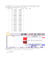
1.10 Viewing PLINK output files . . . . . . .
.
.
.
.
.
.
.
.
.
.
.
.
.
.
.
.
.
.
.
.
.
.
.
.
.
.
.
.
.
.
.
.
.
.
.
.
.
.
.
.
.
.
.
.
.
.
.
.
.
.
.
.
.
.
.
.
.
.
.
.
.
.
.
.
.
.
.
.
.
.
.
.
.
.
.
.
.
.
.
.
.
.
.
.
.
.
.
.
.
.
.
.
.
.
.
.
.
.
.
.
.
.
.
.
.
.
.
.
.
.
.
.
.
.
.
.
.
.
.
.
.
.
.
.
.
.
.
.
.
.
.
.
.
.
.
.
.
.
.
.
.
.
.
.
.
.
.
.
.
.
.
.
.
.
.
.
.
.
.
.
.
.
.
.
.
.
.
.
.
.
.
.
.
.
.
.
.
.
.
.
.
.
.
.
.
.
.
.
.
.
.
.
.
.
.
.
.
.
.
.
.
.
.
.
.
.
.
.
.
.
.
.
.
.
.
.
.
.
.
.
.
.
.
.
.
.
.
.
.
.
.
.
.
.
.
.
.
.
.
.
.
.
.
.
.
.
.
.
.
.
.
.
.
.
.
.
.
.
.
.
.
.
.
.
.
.
.
.
.
.
.
.
.
.
.
.
.
.
.
.
.
.
.
.
.
.
.
.
.
.
.
.
.
.
.
.
.
.
.
.
.
.
.
.
.
.
.
.
.
.
.
.
.
.
.
.
.
.
.
.
.
.
.
.
.
.
.
.
.
.
.
.
.
.
.
.
.
.
.
.
.
.
.
.
.
.
.
.
.
.
.
.
.
.
.
.
.
.
.
.
1
1
1
3
3
3
4
4
5
7
7
8
8
2 A PLINK tutorial
11
2.1 89 HapMap samples and 80K random SNPs . . . . . . . . . . . . . . . . . . . . . . . . . . . . 11
2.2 Using PLINK to analyse these data . . . . . . . . . . . . . . . . . . . . . . . . . . . . . . . . . 12
3 Basic usage / data formats
3.1 Running PLINK . . . . . . . . . . . . . . . . . . . . . . . . . . . .
3.2 PED files . . . . . . . . . . . . . . . . . . . . . . . . . . . . . . . .
3.2.1 Different PED file formats: missing fields . . . . . . . . . .
3.3 MAP files . . . . . . . . . . . . . . . . . . . . . . . . . . . . . . . .
3.3.1 Chromosome codes . . . . . . . . . . . . . . . . . . . . . . .
3.3.2 Allele codes . . . . . . . . . . . . . . . . . . . . . . . . . . .
3.4 Transposed filesets . . . . . . . . . . . . . . . . . . . . . . . . . . .
3.5 Long-format filesets . . . . . . . . . . . . . . . . . . . . . . . . . .
3.5.1 Additional options for long-format files . . . . . . . . . . . .
3.6 Binary PED files . . . . . . . . . . . . . . . . . . . . . . . . . . . .
3.7 Alternate phenotype files . . . . . . . . . . . . . . . . . . . . . . .
3.7.1 Creating a new binary phenotype automatically . . . . . . .
3.7.2 ”Loop association”: automatically testing each group versus
3.8 Covariate files . . . . . . . . . . . . . . . . . . . . . . . . . . . . . .
3.9 Cluster files . . . . . . . . . . . . . . . . . . . . . . . . . . . . . . .
3.10 Set files . . . . . . . . . . . . . . . . . . . . . . . . . . . . . . . . .
. .
. .
. .
. .
. .
. .
. .
. .
. .
. .
. .
. .
all
. .
. .
. .
. . . .
. . . .
. . . .
. . . .
. . . .
. . . .
. . . .
. . . .
. . . .
. . . .
. . . .
. . . .
others
. . . .
. . . .
. . . .
.
.
.
.
.
.
.
.
.
.
.
.
.
.
.
.
.
.
.
.
.
.
.
.
.
.
.
.
.
.
.
.
.
.
.
.
.
.
.
.
.
.
.
.
.
.
.
.
.
.
.
.
.
.
.
.
.
.
.
.
.
.
.
.
.
.
.
.
.
.
.
.
.
.
.
.
.
.
.
.
.
.
.
.
.
.
.
.
.
.
.
.
.
.
.
.
.
.
.
.
.
.
.
.
.
.
.
.
.
.
.
.
.
.
.
.
.
.
.
.
.
.
.
.
.
.
.
.
.
.
.
.
.
.
.
.
.
.
.
.
.
.
.
.
31
31
32
34
35
35
36
37
37
39
41
41
42
43
44
44
45
4 Data management tools
47
4.1 Recode and reorder a sample . . . . . . . . . . . . . . . . . . . . . . . . . . . . . . . . . . . . 47
4.1.1 Transposed genotype files . . . . . . . . . . . . . . . . . . . . . . . . . . . . . . . . . . 48
4.1.2 Additive and dominance components . . . . . . . . . . . . . . . . . . . . . . . . . . . . 48
i
4.2
4.3
4.4
4.5
4.6
4.7
4.8
4.9
4.10
4.11
4.12
4.13
4.14
4.15
4.16
4.17
4.18
4.19
4.20
4.21
4.22
4.23
4.24
4.1.3 Listing by minor allele count . . . . . . . . . . . . . . . . .
4.1.4 Listing by long-format (LGEN) . . . . . . . . . . . . . . . .
4.1.5 Listing by genotype . . . . . . . . . . . . . . . . . . . . . .
Write SNP list files . . . . . . . . . . . . . . . . . . . . . . . . . . .
Update SNP information . . . . . . . . . . . . . . . . . . . . . . . .
Update allele information . . . . . . . . . . . . . . . . . . . . . . .
Force a specific reference allele . . . . . . . . . . . . . . . . . . . .
Update individual information . . . . . . . . . . . . . . . . . . . .
Write covariate files . . . . . . . . . . . . . . . . . . . . . . . . . .
Write cluster files . . . . . . . . . . . . . . . . . . . . . . . . . . . .
Flip DNA strand for SNPs . . . . . . . . . . . . . . . . . . . . . . .
Using LD to identify incorrect strand assignment in a subset of the
Merge two filesets . . . . . . . . . . . . . . . . . . . . . . . . . . . .
Merge multiple filesets . . . . . . . . . . . . . . . . . . . . . . . . .
Extract a subset of SNPs: command line options . . . . . . . . . .
4.13.1 Based on a single chromosome (--chr) . . . . . . . . . . . .
4.13.2 Based on a range of SNPs (--from and --to) . . . . . . . .
4.13.3 Based on single SNP (and window) (--snp and --window)
4.13.4 Based on multiple SNPs and ranges (--snps) . . . . . . . .
4.13.5 Based on physical position (--from-kb, etc) . . . . . . . . .
4.13.6 Based on a random sampling (--thin) . . . . . . . . . . . .
Extract a subset of SNPs: file-list options . . . . . . . . . . . . . .
4.14.1 Based on an attribute file (--attrib) . . . . . . . . . . . .
4.14.2 Based on a set file (--gene) . . . . . . . . . . . . . . . . . .
Remove a subset of SNPs . . . . . . . . . . . . . . . . . . . . . . .
Make missing a specific set of genotypes . . . . . . . . . . . . . . .
Extract a subset of individuals . . . . . . . . . . . . . . . . . . . .
Remove a subset of individuals . . . . . . . . . . . . . . . . . . . .
Filter out a subset of individuals . . . . . . . . . . . . . . . . . . .
Attribute filters for markers and individuals . . . . . . . . . . . . .
Create a SET file based on a list of ranges . . . . . . . . . . . . . .
4.21.1 Options for --make-set . . . . . . . . . . . . . . . . . . . .
Tabulate set membership for all SNPs . . . . . . . . . . . . . . . .
SNP-based quality scores . . . . . . . . . . . . . . . . . . . . . . .
Genotype-based quality scores . . . . . . . . . . . . . . . . . . . . .
5 Summary statistics
5.1 Missing genotypes . . . . . . . . . . . . . . . . . . . . . . .
5.2 Obligatory missing genotypes . . . . . . . . . . . . . . . . .
5.3 Cluster individuals based on missing genotypes . . . . . . .
5.4 Test of missingness by case/control status . . . . . . . . . .
5.5 Haplotype-based test for non-random missing genotype data
5.6 Hardy-Weinberg Equilibrium . . . . . . . . . . . . . . . . .
5.7 Allele frequency . . . . . . . . . . . . . . . . . . . . . . . . .
5.8 Linkage disequilibrium based SNP pruning . . . . . . . . . .
5.9 Mendel errors . . . . . . . . . . . . . . . . . . . . . . . . . .
5.10 Sex check . . . . . . . . . . . . . . . . . . . . . . . . . . . .
5.11 Pedigree errors . . . . . . . . . . . . . . . . . . . . . . . . .
ii
.
.
.
.
.
.
.
.
.
.
.
.
.
.
.
.
.
.
.
.
.
.
.
.
.
.
.
.
.
.
.
.
.
.
.
.
.
.
.
.
.
.
.
.
. . . . .
. . . . .
. . . . .
. . . . .
. . . . .
. . . . .
. . . . .
. . . . .
. . . . .
. . . . .
. . . . .
sample
. . . . .
. . . . .
. . . . .
. . . . .
. . . . .
. . . . .
. . . . .
. . . . .
. . . . .
. . . . .
. . . . .
. . . . .
. . . . .
. . . . .
. . . . .
. . . . .
. . . . .
. . . . .
. . . . .
. . . . .
. . . . .
. . . . .
. . . . .
.
.
.
.
.
.
.
.
.
.
.
.
.
.
.
.
.
.
.
.
.
.
.
.
.
.
.
.
.
.
.
.
.
.
.
.
.
.
.
.
.
.
.
.
.
.
.
.
.
.
.
.
.
.
.
.
.
.
.
.
.
.
.
.
.
.
.
.
.
.
.
.
.
.
.
.
.
.
.
.
.
.
.
.
.
.
.
.
.
.
.
.
.
.
.
.
.
.
.
.
.
.
.
.
.
.
.
.
.
.
.
.
.
.
.
.
.
.
.
.
.
.
.
.
.
.
.
.
.
.
.
.
.
.
.
.
.
.
.
.
.
.
.
.
.
.
.
.
.
.
.
.
.
.
.
.
.
.
.
.
.
.
.
.
.
.
.
.
.
.
.
.
.
.
.
.
.
.
.
.
.
.
.
.
.
.
.
.
.
.
.
.
.
.
.
.
.
.
.
.
.
.
.
.
.
.
.
.
.
.
.
.
.
.
.
.
.
.
.
.
.
.
.
.
.
.
.
.
.
.
.
.
.
.
.
.
.
.
.
.
.
.
.
.
.
.
.
.
.
.
.
.
.
.
.
.
.
.
.
.
.
.
.
.
.
.
.
.
.
.
.
.
.
.
.
.
.
.
.
.
.
.
.
.
.
.
.
.
.
.
.
.
.
.
.
.
.
.
.
.
.
.
.
.
.
.
.
.
.
.
.
.
.
.
.
.
.
.
.
.
.
.
.
.
.
.
.
.
.
.
.
.
.
.
.
.
.
.
.
.
.
.
.
.
.
.
.
.
.
.
50
50
51
51
52
53
53
54
54
56
56
56
58
60
60
60
60
61
61
61
61
62
62
62
63
63
64
64
65
65
66
67
67
68
68
.
.
.
.
.
.
.
.
.
.
.
.
.
.
.
.
.
.
.
.
.
.
.
.
.
.
.
.
.
.
.
.
.
.
.
.
.
.
.
.
.
.
.
.
.
.
.
.
.
.
.
.
.
.
.
.
.
.
.
.
.
.
.
.
.
.
.
.
.
.
.
.
.
.
.
.
.
.
.
.
.
.
.
.
.
.
.
.
.
.
.
.
.
.
.
.
.
.
.
.
.
.
.
.
.
.
.
.
.
.
.
.
.
.
.
.
.
.
.
.
.
71
71
72
74
75
75
77
78
78
79
80
81
.
.
.
.
.
.
.
.
.
.
.
.
.
.
.
.
.
.
.
.
.
.
.
.
.
.
.
.
.
.
.
.
.
.
.
.
.
.
.
.
.
.
.
.
6 Inclusion thresholds
6.0.1 Summary statistics versus
6.0.2 Default threshold values .
6.1 Missing rate per person . . . . .
6.2 Allele frequency . . . . . . . . . .
6.3 Missing rate per SNP . . . . . .
6.4 Hardy-Weinberg Equilibrium . .
6.5 Mendel error rate . . . . . . . . .
.
.
.
.
.
.
.
.
.
.
.
.
.
.
.
.
.
.
.
.
.
.
.
.
.
.
.
.
.
.
.
.
.
.
.
.
.
.
.
.
.
.
.
.
.
.
.
.
.
.
.
.
.
.
.
.
.
.
.
.
.
.
.
.
.
.
.
.
.
.
.
.
.
.
.
.
.
.
.
.
.
.
.
.
.
.
.
.
.
.
.
.
.
.
.
.
.
.
.
.
.
.
.
.
.
.
.
.
.
.
.
.
.
.
.
.
.
.
.
.
.
.
.
.
.
.
.
.
.
.
.
.
.
83
83
83
83
84
84
84
85
7 Population stratification
7.1 IBS clustering . . . . . . . . . . . . . . . . . . . . . . . . . . .
7.2 Permutation test for between group IBS differences . . . . . .
7.3 Constraints on clustering . . . . . . . . . . . . . . . . . . . .
7.4 IBS similarity matrix . . . . . . . . . . . . . . . . . . . . . . .
7.5 Multidimensional scaling plots . . . . . . . . . . . . . . . . .
7.5.1 Speeding up MDS plots: 1. Use the LAPACK library
7.5.2 Speeding up MDS plots: 2. pre-cluster individuals . .
7.6 Outlier detecion diagnostics . . . . . . . . . . . . . . . . . . .
.
.
.
.
.
.
.
.
.
.
.
.
.
.
.
.
.
.
.
.
.
.
.
.
.
.
.
.
.
.
.
.
.
.
.
.
.
.
.
.
.
.
.
.
.
.
.
.
.
.
.
.
.
.
.
.
.
.
.
.
.
.
.
.
.
.
.
.
.
.
.
.
.
.
.
.
.
.
.
.
.
.
.
.
.
.
.
.
.
.
.
.
.
.
.
.
.
.
.
.
.
.
.
.
.
.
.
.
.
.
.
.
.
.
.
.
.
.
.
.
.
.
.
.
.
.
.
.
.
.
.
.
.
.
.
.
.
.
.
.
.
.
.
.
87
87
90
91
93
94
95
95
95
inclusion criteria
. . . . . . . . . .
. . . . . . . . . .
. . . . . . . . . .
. . . . . . . . . .
. . . . . . . . . .
. . . . . . . . . .
.
.
.
.
.
.
.
.
.
.
.
.
.
.
.
.
.
.
.
.
.
.
.
.
.
.
.
.
.
.
.
.
.
.
.
8 IBS/IBD estimation
8.1 Pairwise IBD estimation . . . . . . . . . . . . . . . . . . . . . . .
8.2 Inbreeding coefficients . . . . . . . . . . . . . . . . . . . . . . . .
8.3 Runs of homozygosity . . . . . . . . . . . . . . . . . . . . . . . .
8.4 Segmental sharing: detection of extended haplotypes shared IBD
8.4.1 Check for a homogenous sample . . . . . . . . . . . . . .
8.4.2 Remove very closely related individuals . . . . . . . . . .
8.4.3 Prune the set of SNPs . . . . . . . . . . . . . . . . . . . .
8.4.4 Detecting shared segments (extended, shared haplotypes)
8.4.5 Association with disease . . . . . . . . . . . . . . . . . .
.
.
.
.
.
.
.
.
.
.
.
.
.
.
.
.
.
.
.
.
.
.
.
.
.
.
.
.
.
.
.
.
.
.
.
.
.
.
.
.
.
.
.
.
.
.
.
.
.
.
.
.
.
.
.
.
.
.
.
.
.
.
.
.
.
.
.
.
.
.
.
.
.
.
.
.
.
.
.
.
.
.
.
.
.
.
.
.
.
.
.
.
.
.
.
.
.
.
.
.
.
.
.
.
.
.
.
.
.
.
.
.
.
.
.
.
.
.
.
.
.
.
.
.
.
.
.
.
.
.
.
.
.
.
.
.
.
.
.
.
.
.
.
.
97
97
99
99
102
103
103
103
104
105
9 Association analysis
9.1 Basic case/control association test . . . . . . . . .
9.2 Fisher’s Exact test (allelic association) . . . . . .
9.3 Alternate / full model association tests . . . . . . .
9.4 Stratified analyses . . . . . . . . . . . . . . . . . .
9.5 Testing for heterogeneous association . . . . . . . .
9.6 Hotelling’s T(2) multilocus association test . . . .
9.7 Quantitative trait association . . . . . . . . . . . .
9.8 Genotype means for quantitative traits . . . . . . .
9.9 Quantitative trait interaction (GxE) . . . . . . . .
9.10 Linear and logistic models . . . . . . . . . . . . . .
9.10.1 Basic usage . . . . . . . . . . . . . . . . . .
9.10.2 Covariates and interactions . . . . . . . . .
9.10.3 Flexibly specifying the model . . . . . . . .
9.10.4 Flexibly specifying joint tests . . . . . . . .
9.10.5 Multicollinearity . . . . . . . . . . . . . . .
9.11 Set-based tests . . . . . . . . . . . . . . . . . . . .
9.12 Adjustment for multiple testing: Bonferroni, Sidak,
.
.
.
.
.
.
.
.
.
.
.
.
.
.
.
.
.
.
.
.
.
.
.
.
.
.
.
.
.
.
.
.
.
.
.
.
.
.
.
.
.
.
.
.
.
.
.
.
.
.
.
.
.
.
.
.
.
.
.
.
.
.
.
.
.
.
.
.
.
.
.
.
.
.
.
.
.
.
.
.
.
.
.
.
.
.
.
.
.
.
.
.
.
.
.
.
.
.
.
.
.
.
.
.
.
.
.
.
.
.
.
.
.
.
.
.
.
.
.
.
.
.
.
.
.
.
.
.
.
.
.
.
.
.
.
.
.
.
.
.
.
.
.
.
.
.
.
.
.
.
.
.
.
.
.
.
.
.
.
.
.
.
.
.
.
.
.
.
.
.
.
.
.
.
.
.
.
.
.
.
.
.
.
.
.
.
.
.
.
.
.
.
.
.
.
.
.
.
.
.
.
.
.
.
.
.
.
.
.
.
.
.
.
.
.
.
.
.
.
.
.
.
.
.
.
.
.
.
.
.
.
.
.
.
.
.
.
.
.
.
.
.
.
.
.
.
.
.
.
.
.
.
.
.
.
.
.
.
.
.
.
.
.
.
.
.
.
.
.
.
.
.
107
107
108
108
110
112
112
113
114
114
115
115
117
118
119
119
120
122
iii
. . . . . .
. . . . . .
. . . . . .
. . . . . .
. . . . . .
. . . . . .
. . . . . .
. . . . . .
. . . . . .
. . . . . .
. . . . . .
. . . . . .
. . . . . .
. . . . . .
. . . . . .
. . . . . .
FDR, etc
.
.
.
.
.
.
.
.
.
.
.
.
.
.
.
.
.
.
.
.
.
.
.
.
.
.
.
.
.
.
.
.
.
.
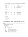
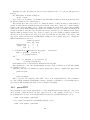
10 Family-based association analysis
10.1 Family-based association (TDT) . . . . . . . . . . . . . . .
10.2 parenTDT . . . . . . . . . . . . . . . . . . . . . . . . . . . .
10.3 Parent of origin analysis . . . . . . . . . . . . . . . . . . . .
10.4 DFAM: family-based association for disease traits . . . . . .
10.5 QFAM: family-based association tests for quantitative traits
.
.
.
.
.
.
.
.
.
.
.
.
.
.
.
.
.
.
.
.
.
.
.
.
.
.
.
.
.
.
.
.
.
.
.
.
.
.
.
.
.
.
.
.
.
.
.
.
.
.
.
.
.
.
.
.
.
.
.
.
.
.
.
.
.
.
.
.
.
.
.
.
.
.
.
.
.
.
.
.
.
.
.
.
.
.
.
.
.
.
125
125
126
127
127
128
11 Permutation procedures
11.0.1 Conceptual overview of permutation procedures . . . . .
11.0.2 Label-swapping and gene-dropping . . . . . . . . . . . .
11.0.3 Adaptive and max(T) permutation . . . . . . . . . . . .
11.0.4 Computational issues . . . . . . . . . . . . . . . . . . .
11.1 Basic (adaptive) permutation procedure . . . . . . . . . . . . .
11.2 Adaptive permutation parameters . . . . . . . . . . . . . . . .
11.3 max(T) permutation . . . . . . . . . . . . . . . . . . . . . . . .
11.4 Gene-dropping permutation . . . . . . . . . . . . . . . . . . . .
11.4.1 Basic within family QTDT . . . . . . . . . . . . . . . .
11.4.2 Discordant sibling test . . . . . . . . . . . . . . . . . . .
11.4.3 parenTDT/parenQTDT . . . . . . . . . . . . . . . . . .
11.4.4 Standard association for singleton, unrelated individuals
11.5 Within-cluster permutation . . . . . . . . . . . . . . . . . . . .
11.6 Generating permuted phenotype filesets . . . . . . . . . . . . .
.
.
.
.
.
.
.
.
.
.
.
.
.
.
.
.
.
.
.
.
.
.
.
.
.
.
.
.
.
.
.
.
.
.
.
.
.
.
.
.
.
.
.
.
.
.
.
.
.
.
.
.
.
.
.
.
.
.
.
.
.
.
.
.
.
.
.
.
.
.
.
.
.
.
.
.
.
.
.
.
.
.
.
.
.
.
.
.
.
.
.
.
.
.
.
.
.
.
.
.
.
.
.
.
.
.
.
.
.
.
.
.
.
.
.
.
.
.
.
.
.
.
.
.
.
.
.
.
.
.
.
.
.
.
.
.
.
.
.
.
.
.
.
.
.
.
.
.
.
.
.
.
.
.
.
.
.
.
.
.
.
.
.
.
.
.
.
.
.
.
.
.
.
.
.
.
.
.
.
.
.
.
.
.
.
.
.
.
.
.
.
.
.
.
.
.
.
.
.
.
.
.
.
.
.
.
.
.
.
.
.
.
.
.
.
.
.
.
.
.
.
.
.
.
.
.
.
.
.
.
.
.
.
.
.
.
.
.
131
131
131
131
132
132
133
133
134
135
135
135
135
136
137
12 Multimarker haplotype tests
12.1 Specification of haplotypes to be estimated . . . . . . . . . . . . . . . . . .
12.2 Precomputed lists of multimarker tests . . . . . . . . . . . . . . . . . . . . .
12.3 Estimating haplotype frequencies . . . . . . . . . . . . . . . . . . . . . . . .
12.4 Testing for haplotype-based case/control and quantitative trait association .
12.5 Haplotype-based association tests with GLMs . . . . . . . . . . . . . . . . .
12.6 Haplotype-based TDT association test . . . . . . . . . . . . . . . . . . . . .
12.7 Imputing multimarker haplotypes . . . . . . . . . . . . . . . . . . . . . . . .
12.8 Tabulating individuals’ haplotype phases . . . . . . . . . . . . . . . . . . . .
.
.
.
.
.
.
.
.
.
.
.
.
.
.
.
.
.
.
.
.
.
.
.
.
.
.
.
.
.
.
.
.
.
.
.
.
.
.
.
.
.
.
.
.
.
.
.
.
.
.
.
.
.
.
.
.
.
.
.
.
.
.
.
.
.
.
.
.
.
.
.
.
.
.
.
.
.
.
.
.
139
139
141
141
141
142
144
144
145
13 LD calculations
13.1 Pairwise LD measures for a single pair of SNPs . . . . . . . . . .
13.2 Pairwise LD measures for multiple SNPs (genome-wide) . . . . .
13.2.1 Filtering the output . . . . . . . . . . . . . . . . . . . . .
13.2.2 Obtaining LD values for a specific SNP versus all others
13.2.3 Obtaining a matrix of LD values . . . . . . . . . . . . . .
13.3 Functions to select tag SNPs for specified SNP sets . . . . . . . .
13.4 Haplotyp block estimation . . . . . . . . . . . . . . . . . . . . . .
.
.
.
.
.
.
.
.
.
.
.
.
.
.
.
.
.
.
.
.
.
.
.
.
.
.
.
.
.
.
.
.
.
.
.
.
.
.
.
.
.
.
.
.
.
.
.
.
.
.
.
.
.
.
.
.
.
.
.
.
.
.
.
.
.
.
.
.
.
.
.
.
.
.
.
.
.
.
.
.
.
.
.
.
.
.
.
.
.
.
.
.
.
.
.
.
.
.
.
.
.
.
.
.
.
.
.
.
.
.
.
.
147
147
147
148
148
148
149
150
14 Conditional haplotype-based association testing
14.1 Basic usage for conditional haplotype-based testing . .
14.2 Specifying the type of test . . . . . . . . . . . . . . . .
14.2.1 Testing a specific haplotype . . . . . . . . . . .
14.2.2 Testing whether SNPs have independent effects
14.2.3 Omnibus test controlling for X . . . . . . . . .
14.3 General specification of haplotype groupings . . . . . .
14.3.1 Manually specifying haplotypes . . . . . . . . .
14.3.2 Manually specifying SNPs . . . . . . . . . . . .
14.4 Covariates and additional SNPs . . . . . . . . . . . . .
.
.
.
.
.
.
.
.
.
.
.
.
.
.
.
.
.
.
.
.
.
.
.
.
.
.
.
.
.
.
.
.
.
.
.
.
.
.
.
.
.
.
.
.
.
.
.
.
.
.
.
.
.
.
.
.
.
.
.
.
.
.
.
.
.
.
.
.
.
.
.
.
.
.
.
.
.
.
.
.
.
.
.
.
.
.
.
.
.
.
.
.
.
.
.
.
.
.
.
.
.
.
.
.
.
.
.
.
.
.
.
.
.
.
.
.
.
.
.
.
.
.
.
.
.
.
.
.
.
.
.
.
.
.
.
.
.
.
.
.
.
.
.
.
153
154
156
156
157
160
162
162
162
163
iv
.
.
.
.
.
.
.
.
.
.
.
.
.
.
.
.
.
.
.
.
.
.
.
.
.
.
.
.
.
.
.
.
.
.
.
.
.
.
.
.
.
.
.
.
.
.
.
.
.
.
.
.
.
.
.
.
.
.
.
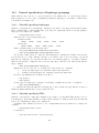
14.5 General setting of linear constraints . . . . . . . . . . . . . . . . . . . . . . . . . . . . . . . . 163
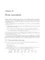
15 Proxy association
15.1 Proxy association: basic usage . . . . . . . . . . . . . . . . . .
15.1.1 Heuristic for selection of proxy SNPs . . . . . . . . . . .
15.1.2 Specifying the type of association test . . . . . . . . . .
15.2 Refining a single SNP association . . . . . . . . . . . . . . . . .
15.3 Automating for multiple references SNPs . . . . . . . . . . . .
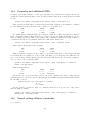
15.4 Providing some degree of robustness to non-random genotyping
16 SNP imputation and association testing
16.1 Basic steps for using PLINK imputation functions . . . . . .
16.1.1 Strand issues . . . . . . . . . . . . . . . . . . . . . . .
16.2 Combined imputation and association analysis of case/control
16.3 Modifying options for basic imputation/association testing . .
16.3.1 Parameters modifying selection of proxies . . . . . . .
16.4 Imputing discrete genotype calls . . . . . . . . . . . . . . . .
16.5 Verbose output options . . . . . . . . . . . . . . . . . . . . .
. . . .
. . . .
. . . .
. . . .
. . . .
failure
. . .
. . .
data
. . .
. . .
. . .
. . .
.
.
.
.
.
.
.
.
.
.
.
.
.
.
.
.
.
.
.
.
.
.
.
.
.
.
.
.
.
.
.
.
.
.
.
.
.
.
.
.
.
.
.
.
.
.
.
.
.
.
.
.
.
.
.
.
.
.
.
.
.
.
.
.
.
.
.
.
.
.
.
.
.
.
.
.
.
.
.
.
.
.
.
.
.
.
.
.
.
.
.
.
.
.
.
.
.
.
.
.
.
.
.
.
.
.
.
.
.
.
.
.
.
.
.
.
.
.
.
.
.
.
.
.
.
.
.
.
.
.
.
.
.
.
.
.
.
.
.
.
.
.
.
.
.
.
.
.
.
.
.
.
.
.
.
.
.
.
.
.
.
.
.
.
.
.
.
.
.
.
.
.
.
.
.
.
165
165
167
170
170
170
171
.
.
.
.
.
.
.
175
175
176
176
177
177
177
179
17 Analysis of dosage data
181
17.1 Basic usage . . . . . . . . . . . . . . . . . . . . . . . . . . . . . . . . . . . . . . . . . . . . . . 181
17.2 Options . . . . . . . . . . . . . . . . . . . . . . . . . . . . . . . . . . . . . . . . . . . . . . . . 182
17.3 Examples of different input format options . . . . . . . . . . . . . . . . . . . . . . . . . . . . . 183
18 Meta-analysis
185
18.1 Basic usage . . . . . . . . . . . . . . . . . . . . . . . . . . . . . . . . . . . . . . . . . . . . . . 185
18.2 Misc. options . . . . . . . . . . . . . . . . . . . . . . . . . . . . . . . . . . . . . . . . . . . . . 187
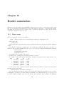
19 Result annotation
189
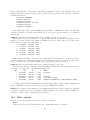
19.1 Basic usage . . . . . . . . . . . . . . . . . . . . . . . . . . . . . . . . . . . . . . . . . . . . . . 189
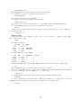
19.2 Misc. options . . . . . . . . . . . . . . . . . . . . . . . . . . . . . . . . . . . . . . . . . . . . . 190
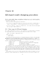
20 LD-based result clumping procedure
20.1 Basic usage for LD-based clumping . . . . . . . . . . . . . . . . . . . .
20.2 Verbose report . . . . . . . . . . . . . . . . . . . . . . . . . . . . . . .
20.2.1 Annotation by SNP details and genomic co-ordinates . . . . . .
20.3 Combining multiple result files (potentially from different SNP panels)
20.4 Selecting the single best proxy . . . . . . . . . . . . . . . . . . . . . .
.
.
.
.
.
.
.
.
.
.
.
.
.
.
.
.
.
.
.
.
.
.
.
.
.
.
.
.
.
.
.
.
.
.
.
.
.
.
.
.
.
.
.
.
.
.
.
.
.
.
.
.
.
.
.
.
.
.
.
.
.
.
.
.
.
193
193
194
195
197
197
21 Gene reporting tool
201
21.1 Basic usage . . . . . . . . . . . . . . . . . . . . . . . . . . . . . . . . . . . . . . . . . . . . . . 201
21.2 Other options . . . . . . . . . . . . . . . . . . . . . . . . . . . . . . . . . . . . . . . . . . . . . 202
22 Epistasis
22.1 SNP x SNP epistasis . . . . . .
22.1.1 A faster epistasis option
22.2 Case-only epistasis . . . . . . .
22.3 Gene-based tests of epistasis . .
.
.
.
.
.
.
.
.
.
.
.
.
.
.
.
.
.
.
.
.
.
.
.
.
.
.
.
.
.
.
.
.
v
.
.
.
.
.
.
.
.
.
.
.
.
.
.
.
.
.
.
.
.
.
.
.
.
.
.
.
.
.
.
.
.
.
.
.
.
.
.
.
.
.
.
.
.
.
.
.
.
.
.
.
.
.
.
.
.
.
.
.
.
.
.
.
.
.
.
.
.
.
.
.
.
.
.
.
.
.
.
.
.
.
.
.
.
.
.
.
.
.
.
.
.
.
.
.
.
.
.
.
.
.
.
.
.
.
.
.
.
203
203
205
205
206
23 R plugin functions
23.1 Basic usage for R plug-ins . . . . .
23.2 Defining the R plug-in function . .
23.3 Example of debugging an R plug-in
23.4 Setting up the Rserve package . . .
.
.
.
.
.
.
.
.
.
.
.
.
.
.
.
.
.
.
.
.
.
.
.
.
.
.
.
.
.
.
.
.
.
.
.
.
.
.
.
.
.
.
.
.
.
.
.
.
.
.
.
.
.
.
.
.
.
.
.
.
.
.
.
.
.
.
.
.
.
.
.
.
.
.
.
.
.
.
.
.
.
.
.
.
.
.
.
.
.
.
.
.
.
.
.
.
.
.
.
.
.
.
.
.
.
.
.
.
.
.
.
.
.
.
.
.
.
.
.
.
.
.
.
.
.
.
.
.
.
.
.
.
207
207
208
209
212
24 SNP annotation database lookup
213
24.1 Basic usage for SNP lookup function . . . . . . . . . . . . . . . . . . . . . . . . . . . . . . . . 213
24.2 Gene-based SNP lookup . . . . . . . . . . . . . . . . . . . . . . . . . . . . . . . . . . . . . . . 215
24.3 Description of the annotation information . . . . . . . . . . . . . . . . . . . . . . . . . . . . . 216
25 SNP simulation routine
25.1 Basic usage . . . . . . . . . . . . . . . . . . . . . . . .
25.2 Specification of LD between marker and causal variant
25.3 Resimulating a sample from the same population . . .
25.4 Simulating a quantitative trait . . . . . . . . . . . . .
.
.
.
.
.
.
.
.
.
.
.
.
.
.
.
.
.
.
.
.
.
.
.
.
.
.
.
.
.
.
.
.
.
.
.
.
.
.
.
.
.
.
.
.
.
.
.
.
.
.
.
.
.
.
.
.
.
.
.
.
.
.
.
.
.
.
.
.
.
.
.
.
.
.
.
.
.
.
.
.
.
.
.
.
.
.
.
.
217
217
218
219
220
26 SNP scoring routine
223
26.1 Basic usage . . . . . . . . . . . . . . . . . . . . . . . . . . . . . . . . . . . . . . . . . . . . . . 223
26.2 Multiple scores from SNP subsets . . . . . . . . . . . . . . . . . . . . . . . . . . . . . . . . . . 224
26.3 Misc. options . . . . . . . . . . . . . . . . . . . . . . . . . . . . . . . . . . . . . . . . . . . . . 224
27 Rare copy number variant (CNV) data
27.1 Basic support for segmental CNV data . . . . . . . . . . . . . . . . .
27.2 Creating MAP files for CNV data . . . . . . . . . . . . . . . . . . . .
27.3 Loading CNV data files . . . . . . . . . . . . . . . . . . . . . . . . .
27.4 Checking for overlapping CNV calls (within the same individual) . .
27.5 Filtering of CNV data based on CNV type . . . . . . . . . . . . . . .
27.6 Filtering of CNV data based on genomic location . . . . . . . . . . .
27.6.1 Defining overlap for partially overlapping CNVs and regions
27.6.2 Filtering by chromosomal co-ordinates . . . . . . . . . . . . .
27.7 Filtering of CNV data based on frequency . . . . . . . . . . . . . . .
27.7.1 Alternative frequency filtering specification . . . . . . . . . .
27.7.2 Miscellaneous commands frequency filtering commands . . .
27.8 Association analysis of segmental CNV data . . . . . . . . . . . . . .
27.9 Association mapping with segmental CNV data . . . . . . . . . . . .
27.10Association mapping with segmental CNV data: regional tests . . .
27.11Association mapping with segmental CNV data: quantitative traits .
27.12Writing new CNV lists . . . . . . . . . . . . . . . . . . . . . . . . . .
27.12.1 Creating UCSC browser CNV tracks . . . . . . . . . . . . . .
27.13Listing intersected genes and regions . . . . . . . . . . . . . . . . . .
27.14Reporting sets of overlapping segmental CNVs . . . . . . . . . . . .
.
.
.
.
.
.
.
.
.
.
.
.
.
.
.
.
.
.
.
.
.
.
.
.
.
.
.
.
.
.
.
.
.
.
.
.
.
.
.
.
.
.
.
.
.
.
.
.
.
.
.
.
.
.
.
.
.
.
.
.
.
.
.
.
.
.
.
.
.
.
.
.
.
.
.
.
.
.
.
.
.
.
.
.
.
.
.
.
.
.
.
.
.
.
.
.
.
.
.
.
.
.
.
.
.
.
.
.
.
.
.
.
.
.
.
.
.
.
.
.
.
.
.
.
.
.
.
.
.
.
.
.
.
.
.
.
.
.
.
.
.
.
.
.
.
.
.
.
.
.
.
.
.
.
.
.
.
.
.
.
.
.
.
.
.
.
.
.
.
.
.
.
.
.
.
.
.
.
.
.
.
.
.
.
.
.
.
.
.
.
.
.
.
.
.
.
.
.
.
.
.
.
.
.
.
.
.
.
.
.
.
.
.
.
.
.
.
.
.
.
.
.
.
.
.
.
.
.
.
.
.
.
.
.
.
.
.
.
.
.
.
.
.
.
.
.
.
.
.
.
.
.
.
.
.
.
.
.
.
.
.
.
.
.
.
.
225
225
226
227
228
228
229
230
230
231
231
232
232
233
234
234
235
235
237
238
28 Common copy number polymorphism (CNP) data
241
28.1 Format for common CNVs (generic variant format) . . . . . . . . . . . . . . . . . . . . . . . . 241
28.2 Association models for combined SNP and common CNV data . . . . . . . . . . . . . . . . . 243
29 Resources available for download
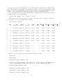
29.1 The Phase 2 HapMap as a PLINK fileset
29.2 Teaching materials and example dataset .
29.3 Multimarker test lists . . . . . . . . . . .
29.4 Gene sets . . . . . . . . . . . . . . . . . .
29.5 Gene range lists . . . . . . . . . . . . . . .
.
.
.
.
.
.
.
.
.
.
vi
.
.
.
.
.
.
.
.
.
.
.
.
.
.
.
.
.
.
.
.
.
.
.
.
.
.
.
.
.
.
.
.
.
.
.
.
.
.
.
.
.
.
.
.
.
.
.
.
.
.
.
.
.
.
.
.
.
.
.
.
.
.
.
.
.
.
.
.
.
.
.
.
.
.
.
.
.
.
.
.
.
.
.
.
.
.
.
.
.
.
.
.
.
.
.
.
.
.
.
.
.
.
.
.
.
.
.
.
.
.
.
.
.
.
.
.
.
.
.
.
.
.
.
.
.
.
.
.
.
.
.
.
.
.
.
245
245
245
246
247
247
29.6 Functional SNP attributes . . . . . . . . . . . . . . . . . . . . . . . . . . . . . . . . . . . . . . 247
30 ID helper
30.1 Example of usage . . . . . . . . . . . . . . . . . . .
30.2 Overview . . . . . . . . . . . . . . . . . . . . . . .
30.3 Consistency checks . . . . . . . . . . . . . . . . . .
30.4 Attributes . . . . . . . . . . . . . . . . . . . . . . .
30.5 Aliases . . . . . . . . . . . . . . . . . . . . . . . . .
30.6 Joint ID specification . . . . . . . . . . . . . . . . .
30.7 Filtering / lookup options . . . . . . . . . . . . . .
30.8 Replace ID schemes in external files . . . . . . . .
30.9 Match multiple files based on IDs . . . . . . . . . .
30.10Quick match multiple files based on IDs, without a
30.11Miscellaneous . . . . . . . . . . . . . . . . . . . . .
30.11.1 The set command . . . . . . . . . . . . . .
30.11.2 List all instances of an ID across files . . . .
. . . . . .
. . . . . .
. . . . . .
. . . . . .
. . . . . .
. . . . . .
. . . . . .
. . . . . .
. . . . . .
dictionary
. . . . . .
. . . . . .
. . . . . .
.
.
.
.
.
.
.
.
.
.
.
.
.
.
.
.
.
.
.
.
.
.
.
.
.
.
.
.
.
.
.
.
.
.
.
.
.
.
.
.
.
.
.
.
.
.
.
.
.
.
.
.
.
.
.
.
.
.
.
.
.
.
.
.
.
.
.
.
.
.
.
.
.
.
.
.
.
.
.
.
.
.
.
.
.
.
.
.
.
.
.
.
.
.
.
.
.
.
.
.
.
.
.
.
.
.
.
.
.
.
.
.
.
.
.
.
.
.
.
.
.
.
.
.
.
.
.
.
.
.
.
.
.
.
.
.
.
.
.
.
.
.
.
.
.
.
.
.
.
.
.
.
.
.
.
.
.
.
.
.
.
.
.
.
.
.
.
.
.
.
.
.
.
.
.
.
.
.
.
.
.
.
.
.
.
.
.
.
.
.
.
.
.
.
.
.
.
.
.
.
.
.
.
.
.
.
.
.
.
.
.
.
.
.
.
.
.
.
.
.
.
.
.
.
.
.
.
.
.
.
.
.
.
.
249
249
251
252
252
253
254
255
255
257
258
258
258
259
31 Miscellaneous
31.1 Command options/modifiers . .
31.2 Output modifiers . . . . . . . .
31.3 Analyses with different species
31.4 File compression . . . . . . . .
31.5 Known issues . . . . . . . . . .
.
.
.
.
.
.
.
.
.
.
.
.
.
.
.
.
.
.
.
.
.
.
.
.
.
.
.
.
.
.
.
.
.
.
.
.
.
.
.
.
.
.
.
.
.
.
.
.
.
.
.
.
.
.
.
.
.
.
.
.
.
.
.
.
.
.
.
.
.
.
.
.
.
.
.
.
.
.
.
.
.
.
.
.
.
.
.
.
.
.
.
.
.
.
.
261
261
261
262
262
263
32 FAQ and Hints
32.1 Can I convert my binary PED fileset back into a standard PED/MAP fileset? . . . . .
32.2 To speed up input of a large fileset . . . . . . . . . . . . . . . . . . . . . . . . . . . . .
32.3 Why are no indidividuals included in the analysis? . . . . . . . . . . . . . . . . . . . .
32.4 Why are my results different from an analysis using program X? . . . . . . . . . . . . .
32.5 How large a file can PLINK handle? . . . . . . . . . . . . . . . . . . . . . . . . . . . .
32.6 Why does my linear/logistic regression output have all NA’s? . . . . . . . . . . . . . . .
32.7 What kind of computer do I need to run PLINK? . . . . . . . . . . . . . . . . . . . .
32.8 Can I analyse multiple phenotypes in a single run (e.g. for gene expression datasets)?
32.9 How does PLINK handle the X chromosome in association tests? . . . . . . . . . . . .
32.10Can/why can’t gPLINK perform a particular PLINK command? . . . . . . . . . . . .
32.11When I include covariates with --linear or --logistic, what do the p-values mean?
.
.
.
.
.
.
.
.
.
.
.
.
.
.
.
.
.
.
.
.
.
.
.
.
.
.
.
.
.
.
.
.
.
.
.
.
.
.
.
.
.
.
.
.
265
265
265
266
266
266
267
267
268
268
268
269
.
.
.
.
.
.
.
.
.
.
.
.
.
.
.
.
.
.
.
.
.
.
.
.
.
.
.
.
.
.
.
.
.
.
.
.
.
.
.
.
.
.
.
.
.
.
.
.
.
.
.
.
.
.
.
.
.
.
.
.
.
.
.
.
.
.
.
.
.
.
.
.
.
.
.
.
.
.
.
.
A Reference Tables
271
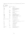
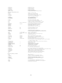
A.1 Options . . . . . . . . . . . . . . . . . . . . . . . . . . . . . . . . . . . . . . . . . . . . . . . . 272
A.2 Output files (alphabetical listing: not up-to-date) . . . . . . . . . . . . . . . . . . . . . . . 277
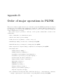
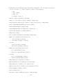
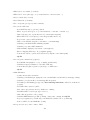
B Order of major operations in PLINK
279
vii
viii
Chapter 1
Getting started with PLINK
This page contains some important information on learning to use PLINK and how to handle any problems
you encounter.
We suggest that after downloading PLINK you first try the tutorial. This will familiarize you with the
basic PLINK commands.
1.1
Citing PLINK
If you use PLINK in any published work, please cite both the software (as an electronic resource/URL) and
the manuscript describing the methods.
Package:
PLINK (including version number)
Author:
Shaun Purcell
URL:
http://pngu.mgh.harvard.edu/purcell/plink/
Purcell S, Neale B, Todd-Brown K, Thomas L, Ferreira MAR,
Bender D, Maller J, Sklar P, de Bakker PIW, Daly MJ & Sham PC (2007)
PLINK: a toolset for whole-genome association and population-based
linkage analysis. American Journal of Human Genetics, 81.
1.2
Reporting problems, bugs and questions
If you have any problems with PLINK or would like to report a bug, please follow these steps:
PLEASE READ THIS SECTION BEFORE E-MAILING!
When an analysis does not report the results you expect, or when PLINK seemingly gives different
answers to previous versions or to other software packages, or the last time you ran it, etc, please feel me to
e-mail me
plink AT chgr DOT mgh DOT harvard DOT edu
but also please consider the following before doing so:
• Please first check the Frequently Asked Questions list to see if your question has already been answered
• Please check the LOG file, it often contains important information. For example, did it filter out
some individuals based on genotyping rate or missing phenotype/sex information which you were not
expecting?
• Please check the format of your data: is it plain text? does each file have the correct number of rows,
etc. Are the missing value codes appropriate?
1
• Please recheck the web-documentation: sometimes the syntax of an option may change.
• If the above steps do not resolve your problem, then please e-mail me plink AT chgr dot mgh dot
harvard dot edu (this is different from the mailing list – i.e. your e-mail will only be sent to me,
not the whole list). The more specific your e-mail, the easier it will be for me to diagnose any problem
or error. Please include:
– The whole LOG file(s)
– The type of machine you were using
– Ideally, please try to make some reduced dataset that replicates the problem that you are able to
send to me in a ZIP file, so that I will be able to recreate the problem; any data sent to me for
these purposes will be immediately deleted after I have resolved the problem.
HINT The more of the above steps you follow, the more likely you are to receive a timely, useful response!
If you haven’t heard within a week or so, please feel free to send a reminder e-mail...
IMPORTANT I am willing and able to advise on the use of specific features implemented in PLINK: to
diagnose whether they are working as intended and to give a generic description of a procedure or method,
if it is unclear from the web documentation. I’m afraid I will not necessarily be able to give specific advice
on any one particular dataset, why you should use one method over another, what it all means, etc...
2
This page contains some important information regarding how to set up and use PLINK. Individuals
familiar with using command line programs can probably skip most of this page.
1.3
Download
PLINK is now available for free download. Below are links to ZIP files containing binaries compilied on
various platforms as well as the C/C++ source code. Linux/Unix users should download the source code
and compile (see notes below).
These downloads also contain a version of gPLINK, an (optional) GUI for PLINK. Please see these pages
for instructions on use of gPLINK.
Remember This release is considered a stable release, although please remember that we cannot guarantee
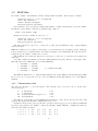
that it, just like most computer programs, does not contain bugs...
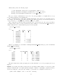
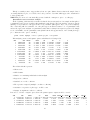
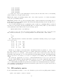
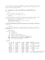
Platform File Version
Linux (x86 64)
Linux (i686)
MS-DOS
Apple Mac (PPC)
Apple Mac (Intel)
C/C++ source (.zip)
plink-1.07-x86 64.zip http://pngu.mgh.harvard.edu/∼purcell/dist/plink- 1.07- x86\ 64.zip
plink-1.07-i686.zip http://pngu.mgh.harvard.edu/∼purcell/dist/plink- 1.07- i686.zip
plink-1.07-dos.zip http://pngu.mgh.harvard.edu/∼purcell/dist/plink- 1.07- dos.zip
plink-1.07-mac.zip http://pngu.mgh.harvard.edu/∼purcell/dist/plink- 1.07- mac.zip
plink-1.07-mac-intel.zip http://pngu.mgh.harvard.edu/∼purcell/dist/plink- 1.07- mac- intel.zip
plink-1.07-src.zip http://pngu.mgh.harvard.edu/∼purcell/dist/plink- 1.07- src.zip
v1.07
v1.07 (to be posted next week)
v1.07 (to be posted later today, 30-Oct)
v1.07 (to be posted next week)
v1.07
v1.07
One more thing... If you download PLINK please either join the very low-volume e-mail list (link from
Introduction page) or drop an e-mail to plink AT chgr dot mgh dot harvard dot edu letting me know
you’ve downloaded a copy.
For old versions of PLINK please visit the archive.
Debian users PLINK is available as a Debian package, see these notes http://packages.debian.org/
sid/plink. Note, the executable is named snplink in the Debian plink package.
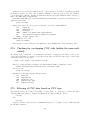
1.4
Development version source code
You can download the very latest development source code in this ZIP file http://pngu.mgh.harvard.edu/
∼purcell/dist/plink-latest.zip. This is really, strongly not recommended for most users. The
code posted here could change on a daily basis and is not versioned.
Development source code versions have a p suffix, meaning pre-release. For example, if the current release
is 1.04, the next stable release will be 1.05 and the development code will be 1.05p. Note that 1.05 may
differ from 1.05p and as noted before, from day-to-day the 1.05 development code may change in any case.
The principle reason for including the source code here is to allow access for specific users to specific,
new features. These features are described here.
1.5
General installation notes
The PLINK executable file should be placed in either the current working directory or somewhere in the
command path. This means that typing
plink
or
./plink
at the command line prompt will run PLINK, no matter which current directory you happen to be in.
PLINK is a command line program – clicking on an icon with the mouse will get you nowhere.
Below, on this page, is a general overview of how to use the command line to run PLINK. The next
sections give details about how to install PLINK on different platforms.
3
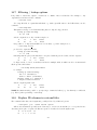
1.6
Windows/MS-DOS notes
Unzipping the downloaded ZIP file should reveal a single executable program plink.exe. The Windows/MSDOS version of PLINK is also a command line program, and is run by typing
plink options...
not by clicking on the icon with the mouse. Open a DOS windows by selecting ”Command Prompt”
from the start menu, or entering ”command” or ”cmd” in the ”Run...” option of the start menu.
The folders c:\windows\ or c:\winnt\ are typically in the path, so these are good places to copy the
file plink.exe to. You can copy the plink.exe file using Windows, as you would copy-and-paste any file
(e.g. using the right-button menu or the keyboard shortcuts control-C (paste) and control-V (paste).
Alternatively, if you know that you will only ever run PLINK on files in a single folder, then you can paste
plink.exe into that folder, e.g. C:\work\genetics\. The disadvantage of this approach is that PLINK will
not be available from the command line if you are in a folder other than this one.
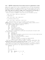
Once you have copied plink.exe to the correct location, you can test whether or not PLINK is available
(i.e. in your command path) by simply typing
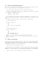
plink
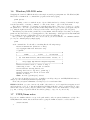
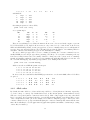
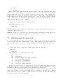
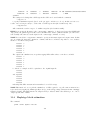
at the command line. You should see something like the following message:
Microsoft Windows XP [Version 5.1.2600]
(C) Copyright 1985-2001 Microsoft Corp.
C:\>plink
@----------------------------------------------------------@
|
PLINK!
|
v0.99l
|
27/Jul/2006
|
|----------------------------------------------------------|
| (C) 2006 Shaun Purcell, GNU General Public License, v2 |
|----------------------------------------------------------|
|
http://pngu.mgh.harvard.edu/purcell/plink/
|
@----------------------------------------------------------@
Web-based version check ( --noweb to skip )
Connecting to web... OK, v0.99l is current
*** Pre-Release Testing Version ***
Writing this text to log file [ plink.log ]
Analysis started: Fri Jul 28 10:07:57 2006
Options in effect:
ERROR: No file [ plink.ped ] exists.
Do not worry about this error message – normally you would specify your own PED/MAP file names to
analyse (i.e. the default input filename is plink.ped).
Please ask your system administrator for help if you do not understand this.
HINT In MS-DOS, you can to increase the width of the window to avoid output lines wrapping around
and being hard to read. To do this under Windows XP DOS: right click on the top title/menu bar of the
window and select Properties / Layout / Window Size / Width – increse the width value to a larger value
(e.g. 120, or as large as possible without the window getting too big to fit on your screen!).
1.7
UNIX/Linux notes
If you are not familiar with the concept of the path variable, ask your system administrator to help. In a
UNIX/Linux environment, this would mean either copying the PLINK executable to a folder such as
/usr/local/bin/
or
4
~
/bin/
assuming these directories exist and are in the path. To see which directories are in the path, typing
$PATH
at the command prompt will often work. To create a directory, say called bin in your home directory
and add it to the path, try
mkdir ~
/bin
export PATH=$PATH:~
/bin/
although this will depend on which shell you are using. Some shells do not include the current directory
in the path: in this case, you might need to prefix all PLINK commands with the characters ./, e.g.
./plink --file mydata --assoc
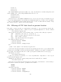
1.8
Source code compilation
PLINK is also distributed as C/C++ source code, which you can compile for your particular system using
any standard C/C++ compile. Download the .zip or .tar.gz files and perform the following steps:
tar -xzvf plink-0.99s-src.tar.gz
or
unzip plink-0.99s-src.zip
or use a graphical tool such as WinZip to extract the contents of the archive. This should create a
directory called
plink-0.99s-src
(the exact version number might be different, of course). On the command line, move to that dirctory
and simply type make :
cd plink-0.99s
You will need a C/C++ compiler installed on your system for the next step. Linux distributions will
include gcc/g++ by default. Ask your system administrator about installing a C/C++ compiler if you do
not have one already (Windows, MS-DOS users).
Hint PLINK has not been exhaustively tested on different compilers. We sugest you use a recent download
of MinGW for Windows, or at least gcc 4.1.
WARNING We suggest using the most recent stable release of the compiler available on your platform
to avoid compilation problems. For most platforms this means gcc 4.2 as of writing this. Some issues with
specific older compiler and specific platforms have been detected, e.g. gcc 3.3.3 on a SGI Altix 3700 system.
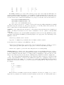
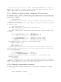
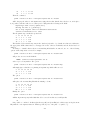
Use a standard text editor such as emacs, pico or WordPad to edit the Makefile to suit your particular
platform: the top of the Makefile should look like this:
# --------------------------------------------------------------------#
#
Makefile for PLINK
#
#
Supported platforms
#
Unix / Linux
LINUX
#
Windows
WIN
#
Mac
MAC
5
#
Solaris
SOLARIS
#
#
Compilation options
#
R plugins
WITH R PLUGINS
#
Web-based version check
WITH WEBCHECK
#
Ensure 32-bit binary
FORCE 32BIT
#
(Ignored)
WITH ZLIB
#
Link to LAPACK
WITH LAPACK
#
Force dynamic linking
FORCE DYNAMIC
#
# --------------------------------------------------------------------# Set this variable to either UNIX, MAC or WIN
SYS = UNIX
# Leave blank after "=" to disable; put "= 1" to enable
WITH R PLUGINS = 1
WITH WEBCHECK = 1
FORCE 32BIT =
WITH ZLIB =
WITH LAPACK =
FORCE DYNAMIC =
# Put C++ compiler here; Windows has it’s own specific version
CXX UNIX = g++
CXX WIN = c:\bin\mingw\bin\mingw32-g++.exe
# Any other compiler flags here ( -Wall, -g, etc)
CXXFLAGS =
# Misc
LIB LAPACK = /usr/lib/liblapack.so.3
# -------------------------------------------------------------------# Do not edit below this line
# -------------------------------------------------------------------The steps to edit this:
• Change the SYS variable to your platform, e.g. WIN for Windows
• For the next set of options, put either a 1 or leave blank to turn on or off these options, respectively.
– WITH R PLUGINS This enables support for R plugins using Rserve as described here. Currently
this only works for Unix-based machines.
– If you want to disable the web-based version check option (not recommended) or if compilation
fails with this on, you might try removing the 1 after WITH WEBCHECK
– When compiling on a 64-bit machine, this option, FORCE 32BIT, can force (when set) a 32 bit
binary (assumes all necessary libraries, etc) are in place
– Other options listed here are described below.
• Edit the CXX * variable to point to the C/C++ compiler you wish to use
• To pass any extra commands to the compiler (e.g. location of libraries, etc), you can edit CXX FLAGS
6
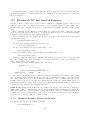
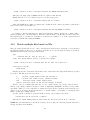
1.8.1
LAPACK support
As described here, linking to the LAPACK library can greatly speed up MDS analysis of population stratificaiton. This may take a little tweaking:
• Obtain and compile LAPACK, here http://www.netlib.org/lapack/. This requires the gfortran
http://gcc.gnu.org/fortran/ compiler. I cannot assist in any technical difficulties you have with
this: ask you IT staff. It is quite possible that LAPACK is already installed somewhere in your
institution.
• Determine where the LAPACK library file is located, and whether it is a shared (e.g. liblapack.so.3)
or static (e.g. lapack LINUX.a) library. (Libraries ending .a are static; libraries ending .so.* are
shared, or dynamically linked. If the LAPACK libraries are shared libraries, then set the FORCE DYNAMIC
flag to have 1 after it in the PLINK Makefile.
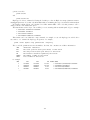
• Set the variable LIB LAPACK to point to the LAPACK libraries. This may vary by machine and the
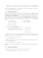
precise installation of LAPACK. For example, on one machine, I have three static LAPACK libraries
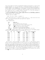
in the directory I compiled LAPACK in:
~
/src/plink> ls ../lapack-3.2/*a
../lapack-3.2/blas LINUX.a
../lapack-3.2/lapack LINUX.a
../lapack-3.2/tmglib LINUX.a
In this case, set (all one line)
LIB LAPACK = ../lapack-3.2/lapack LINUX.a
LIB LAPACK += ../lapack-3.2/blas LINUX.a
LIB LAPACK += ../lapack-3.2/tmglib LINUX.a
On this machine, it was also necessary to add
LIB LAPACK += -lgfortran
On a different (Linux) machine, the LAPACK library was a shared one, in /usr/lib/liblapack.so.3,
that worked as a single file. In this case, the necessary changes were to set the WITH LAPACK and
FORCE DYNAMIC flags, then set
LIB LAPACK = /usr/lib/liblapack.so.3
Doubtless there is a better way to configure this, but for now I present the above as a quick-fix way of
achieving LAPACK support. A little tweaking by somebody who knows what they are doing should suffice.
I will not be able to provide detailed help for platforms I am unfamiliar with: you are on your own I’m
afraid! You are likely to see some linker errors when compiling if things are not right.
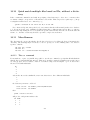
1.8.2
Starting compilation
You should then just type
make
and PLINK should (hopefully) start compiling. You should use GNU version, which is sometimes called
gmake on some platforms (e.g. FreeBSD). It is also possible that you have installed make but it is not in
your path and/or your version of make.exe is called something slightly different, in which case use the full
path, e.g. change the following to suit your system:
c:\mingw\bin\mingw32-make
7
NOTE Often problems in compilation will reflect system-specific / compiler-specific problems: unfortunately, we are not able to give detailed advice on how to do this. If things do not work and you are unsure,
you will need to enlist the help of your systems/IT department.
You should see something like the following output (abbreviated)
g++ -O3 -I. -DUNIX -static -c plink.cpp
g++ -O3 -I. -DUNIX -static -c options.cpp
g++ -O3 -I. -DUNIX -static -c input.cpp
...
g++ -O3 -static -o plink plink.o options.o input.o binput.o
helper.o genome.o snpfilter.o indfilter.o locus.o multi.o
regress.o crandom.o cluster.o output.o informative.o affpair.o
assoc.o bins.o epi.o phase.o trio.o sharing.o genepi.o sets.o
perm.o mh.o genedrop.o gxe.o merge.o hotel.o multiple.o
After a minute or so, this will have created an executable binary file called plink (or plink.exe for
Windows/MSDOS users).
1.9
Running PLINK from the command line
A typical session might involve running several commands, e.g. to produce summary statistics on missing
data, to exclude some SNPs based on these results, to run an association analysis. Each command involves
a separate instantiation of plink – note that PLINK does not remember any parameter settings between
different runs or store any other information. In otherwords, if you want to perform two association tests
with different PED files, but only including SNPs that are above a certain minor allele frequency in both
runs, you would use the following:
plink --ped file1.ped --map file1.map --maf 0.05 --assoc
plink --ped file2.ped --map file2.map --maf 0.05 --assoc
In otherwords, the following sequence would not work:
plink --ped file1.ped --map file1.map --maf 0.05
plink --ped file1.ped --map file1.map --assoc
MAF returns to default 0.01
plink --ped file2.ped --map file2.map --assoc
As above
1.10
Viewing PLINK output files
UPDATE We are developing the tool gPLINK to integrate PLINK with Haploview http://www.broad.
mit.edu/mpg/haploview/. Haploview 4.0 provides a number of features for viewing, filtering and plotting
PLINK results files. This is intended to supplant the methods suggested below.
All the output files that PLINK generates are plain-text, space-delimited files. Most files will have the
same number of fields per line and will have the field names in the first line, facilitating use of a spreadsheet
or statistics package to view and process the results.
For small results files, simply printing the files to the terminal or viewing in a text-editor should work
well. In Windows/MS-DOS use the type command, e.g.
type mydata.assoc
8
to view a results file. Alternatively, you can call up WordPad from the command line as follows:
write mydata.assoc
If you are using a Unix/Linux system, then commands such as cat, more or less can be used to display
the results; alternatively text-editors such as pico, emacs or vi.
Of course, Unix/Linux users also have available the entire range of text-processing tools (grep, gawk,
perl, sort, head, etc) and shell-scripting tools, as well as powerful text-editors (emacs, etc) that are ideal
for processing very large result files. Another alternative is to use a statistics package such as the R package
www.r-project.org which will provide powerful visualisation tools also.
Windows/MS-DOS users have fewer options for handling very large results files: For moderate size
files (e.g. up to 50K SNPs), you could use Excel. For larger files, you can either install cygwin http:
//www.cygwin.com/ to provide a Linux-like environment, or use a statistics package such as the R package
www.r-project.org.
Personal opinion... Although a MS-DOS version of PLINK is supported, we would, in general, advise any
any researchers planning on performing many large-scale analyses to look into adopting a Linux environment,
if they are not already using this.
9
10
Chapter 2
A PLINK tutorial
In this tutorial, we will consider using PLINK to analyse example data: randomly selected genotypes (approximately 80,000 autosomal SNPs) from the 89 Asian HapMap individuals. A phenotype has been simulated
based on the genotype at one SNP. In this tutorial, we will walk through using PLINK to work with the
data, using a range of features: data management, summary statistics, population stratification and basic
association analysis.
NOTE These data do not, of course, represent a realistic study design or a realistic disease model. The
point of this exercise is simply to get used to running PLINK.
2.1
89 HapMap samples and 80K random SNPs
The first step is to obtain a working copy of PLINK and of the example data files.
• Make sure you have PLINK installed on your machine (see these instructions).
• Download the example data archive file which contains the genotypes, map files and two extra phenotype files, described below (zipped, approximately 2.8M)
• Create a new folder/directory on your machine, and unzip the file you downloaded (called hapmap1.zip)
into this folder.
HINT! If you are a Windows user who is unsure how to do this, follow this link
¡hr width=25%¿ Two phenotypes were generated: a quantitative triat and a disease trait (affection status,
coded 1=unaffected, 2=affected), based on a median split of the quantitative trait. The quantitative trait
was generated as a function of three simple components:
• A random component
• Chinese versus Japanese identity
• A variant on chromosome 2, rs2222162
Remember, this model is not intended to be realistic. The following contingency table shows the joint
distribution of disease and subpopulation:
Control
Case
Chinese
34
11
Japanese
11
33
which shows a strong relationship between these two variables. The next table shows the association
between the variant rs2222162 and disease:
11
Control
Case
Genotype
11
12
17
22
3
19
22
6
22
Again, the strong association is clear. Note that the alleles have been recoded as 1 and 2 (this is not
necessary for PLINK to work, however – it can accept any coding for SNPs).
In summary, we have a single causal variant that is associated with disease. Complicating factors are that
this variant is one of 83534 SNPs and also that there might be some degree of confounding of the SNP-disease
associations due to the subpopulation-disease association – i.e. a possibility that population stratification
effects will exist. Even though we might expect the two subpopulations to be fairly similar from an overall
genetic perspective, and even though the sample size is small, this might still lead to an increase in false
positive rates if not controlled for.
We will use the affection status variable as the default variable for analysis (i.e. the sixth column in
the PED file). The quantitative trait is in a separate alternate phenotype file, qt.phe. The file pop.phe
contains a dummy phenotype that is coded 1 for Chinese individuals and 2 for Japanese individuals. We
will use this in investigating between-population differences. You can view these alternate phenotype files
in any text editor.
In this tutorial dataset we focus on autosomal SNPs for simplicity, although PLINK does provide support
for X and Y chromosome SNPs for a number of analyses. See the main documentation for further information.
2.2
Using PLINK to analyse these data
This tutorial is intended to introduce some of PLINK’s features rather than provide exhaustive coverage of
them. Futhermore, it is not intended as an analysis plan for whole genome data, or to represent anything
close to ’best practice’.
These hyperlinks show an overview of topics:
• Getting started
• Making a binary PED file
• Working with the binary PED file
• Summary statistics: missing rates
• Summary statistics: allele frequencies
• Basic association analysis
• Genotypic association models
• Stratification analysis
• Association analysis, accounting for clusters
• Quantitative trait association analysis
• Extracting a SNP of interest
Getting started
Just typing plink and specifying a file with no further options is a good way to check that the file is
intact, and to get some basic summary statistics about the file.
plink --file hapmap1
12
The --file option takes a single parameter, the root of the input file names, and will look for two files:
a PED file and a MAP file with this root name. In otherwords, --file hapmap1 implies hapmap1.ped and
hapmap1.map should exist in the current directory.
HINT! It is possible to specify files outside of the current directory, and to have the PED and MAP files
have different root names, or not end in .ped and .map, by using the --ped and --map options.
PED and MAP files are plain text files; PED files contain genotype information (one person per row)
and MAP files contain information on the name and position of the markers in the PED file. If you are not
familiar with the file formats required for PED and MAP files, please consult this page.
The above command should generate something like the following output in the console window. It will
also save this information to a file called plink.log.
@----------------------------------------------------------@
|
PLINK!
|
v0.99l
|
27/Jul/2006
|
|----------------------------------------------------------|
| (C) 2006 Shaun Purcell, GNU General Public License, v2 |
|----------------------------------------------------------|
|
http://pngu.mgh.harvard.edu/purcell/plink/
|
@----------------------------------------------------------@
Web-based version check ( --noweb to skip )
Connecting to web... OK, v0.99l is current
*** Pre-Release Testing Version ***
Writing this text to log file [ plink.log ]
Analysis started: Mon Jul 31 09:00:11 2006
Options in effect:
--file hapmap1
83534 (of 83534) markers to be included from [ hapmap1.map ]
89 individuals read from [ hapmap1.ped ]
89 individuals with nonmissing phenotypes
Assuming a binary trait (1=unaff, 2=aff, 0=miss)
Missing phenotype value is also -9
Before frequency and genotyping pruning, there are 83534 SNPs
Applying filters (SNP-major mode)
89 founders and 0 non-founders found
0 of 89 individuals removed for low genotyping ( MIND > 0.1 )
859 SNPs failed missingness test ( GENO > 0.1 )
16994 SNPs failed frequency test ( MAF < 0.01 )
After frequency and genotyping pruning, there are 65803 SNPs
Analysis finished: Mon Jul 31 09:00:19 2006
The information contained here can be summarized as follows:
• A banner showing copyright information and the version number – the web-based version check shows
that this is an up-to-date version of PLINK and displays a message that v0.99l is a pre-release testing
version.
• A message indicating that the log file will be saved in plink.log. The name of the output file can be
changed with the --out option – e.g. specifying --out anal1 will generate a log file called anal1.log
instead.
• A list of the command options specified is given next: in this case it is only a single option, --file
hapmap1. By keeping track of log files, and naming each analysis with its own --out name, it makes
it easier to keep track of when and how the different output files were generated.
13
• Next is some information on the number of markers and individuals read from the MAP and PED
file. In total, just over 80,000 SNPs were read in from the MAP file. It is written "...83534 (of
83534)..." because some SNPs might be excluded (by making the physical position a negative number
in the MAP file), in which case the first number would indicate how many SNPs are included. In this
case, all SNPs are read in from the PED file. We also see that 89 individuals were read in from the
PED file, and that all these individuals had valid phenotype information.
• Next, PLINK tells us that the phenotype is an affection status variable, as opposed to a quantitative
trait, and lets us know what the missing values are.
• The next stage is the filtering stage – individuals and/or SNPs are removed on the basis of thresholds.
Please see this page for more information on setting thresholds. In this case we see that no individuals
were removed, but almost 20,000 SNPs were removed, based on missingness (859) and frequency
(16994). This particularly high proportion of removed SNPs is based on the fact that these are
random HapMap SNPs in the Chinese and Japanese samples, rather than pre-selected markers on a
whole-genome association product: there will be many more rare and monomorphic markers here than
one would normally expect.
• Finally, a line is given that indicates when this analysis finished. You can see that it took 8 seconds
(on my machine at least) to read in the file and apply the filters.
If other analyses had been requsted, then the other output files generated would have been indicated in the
log file. All output files that PLINK generates have the same format: root.extension where root is, by
default, ”plink” but can be changed with the --out option, and the extension will depend on the type of
output file it is (a complete list of extensions is given here).
Making a binary PED file
The first thing we will do is to make a binary PED file. This more compact representation of the data
saves space and speeds up subsequent analysis. To make a binary PED file, use the following command.
plink --file hapmap1 --make-bed --out hapmap1
If it runs correctly on your machine, you should see the following in your output:
above as before
...
Before frequency and genotyping pruning, there are 83534 SNPs
Applying filters (SNP-major mode)
89 founders and 0 non-founders found
0 SNPs failed missingness test ( GENO > 1 )
0 SNPs failed frequency test ( MAF < 0 )
After frequency and genotyping pruning, there are 83534 SNPs
Writing pedigree information to [ hapmap1.fam ]
Writing map (extended format) information to [ hapmap1.bim ]
Writing genotype bitfile to [ hapmap1.bed ]
Using (default) SNP-major mode
Analysis finished: Mon Jul 31 09:10:05 2006
There are several things to note:
• When using the --make-bed option, the threshold filters for missing rates and allele frequency were
automatically set to exclude nobody. Although these filters can be specified manually (using --mind,
--geno and --maf) to exclude people, this default tends to be wanted when creating a new PED or
binary PED file. The commands --extract / --exclude and --keep / --remove can also be applied
at this stage.
14
• Three files are created with this command – the binary file that contains the raw genotype data
hapmap1.bed but also a revsied map file hapmap1.bim which contains two extra columns that give the
allele names for each SNP, and hapmap1.fam which is just the first six columns of hapmap1.ped. You
can view the .bim and .fam files – but do not try to view the .bed file. None of these three files should
be manually editted.
If, for example, you wanted to create a new file that only includes individuals with high genotyping (at
least 95% complete), you would run:
plink --file hapmap1 --make-bed --mind 0.05 --out highgeno
which would create files
highgeno.bed
highgeno.bim
highgeno.fam
Working with the binary PED file
To specify that the input data are in binary format, as opposed to the normal text PED/MAP format,
just use the --bfile option instead of --file. To repeat the first command we ran (which just loads the
data and prints some basic summary statistics):
plink --bfile hapmap1
Writing this text to log file [ plink.log ]
Analysis started: Mon Jul 31 09:12:08 2006
Options in effect:
--bfile hapmap1
Reading map (extended format) from [ hapmap1.bim ]
83534 markers to be included from [ hapmap1.bim ]
Reading pedigree information from [ hapmap1.fam ]
89 individuals read from [ hapmap1.fam ]
89 individuals with nonmissing phenotypes
Reading genotype bitfile from [ hapmap1.bed ]
Detected that binary PED file is v1.00 SNP-major mode
Before frequency and genotyping pruning, there are 83534 SNPs
Applying filters (SNP-major mode)
89 founders and 0 non-founders found
0 of 89 individuals removed for low genotyping ( MIND > 0.1 )
859 SNPs failed missingness test ( GENO > 0.1 )
16994 SNPs failed frequency test ( MAF < 0.01 )
After frequency and genotyping pruning, there are 65803 SNPs
Analysis finished: Mon Jul 31 09:12:10 2006
The things to note here:
• That three files hapmap1.bim, hapmap1.fam and hapmap1.bed were loaded instead of the usual two
files. That is, hapmap1.ped and hapmap1.map are not used in this analysis, and could in fact be deleted
now.
• The data are loaded in much more quickly – based on the timestamp at the beginning and end of the
log output, this took 2 seconds instead of 10.
Summary statistics: missing rates
Next, we shall generate some simple summary statistics on rates of missing data in the file, using the
--missing option:
plink --bfile hapmap1 --missing --out miss stat
15
which should generate the following output:
...
0 of 89 individuals removed for low genotyping ( MIND > 0.1 )
Writing individual missingness information to [ miss stat.imiss ]
Writing locus missingness information to [ miss stat.lmiss ]
...
Here we see that no individuals were removed for low genotypes (MIND > 0.1 implies that we accept
people with less than 10 percent missingness).
The per individual and per SNP (after excluding individuals on the basis of low genotyping) rates are
then output to the files miss stat.imiss and miss stat.lmiss respectively. If we had not specified an
--out option, the root output filename would have defaulted to ”plink”.
These output files are standard, plain text files that can be viewed in any text editor, pager, spreadsheet
or statistics package (albeit one that can handle large files). Taking a look at the file miss stat.lmiss, for
example using the more command which is present on most systems:
more miss stat.lmiss
we see
CHR
1
1
1
1
1
1
1
1
1
...
SNP
rs6681049
rs4074137
rs7540009
rs1891905
rs9729550
rs3813196
rs6704013
rs307347
rs9439440
N MISS
0
0
0
0
0
0
2
12
2
F MISS
0
0
0
0
0
0
0.0224719
0.134831
0.0224719
That is, for each SNP, we see the number of missing individuals (N MISS) and the proportion of individuals
missing (F MISS). Similarly:
more miss stat.imiss
we see
FID
HCB181
HCB182
HCB183
HCB184
HCB185
HCB186
HCB187
...
IID MISS PHENO
1
N
1
N
1
N
1
N
1
N
1
N
1
N
N MISS
671
1156
498
412
329
1233
258
F MISS
0.00803266
0.0138387
0.00596164
0.00493212
0.00393852
0.0147605
0.00308856
The final column is the actual genotyping rate for that individual – we see the genotyping rate is very
high here.
HINT If you are using a spreadsheet package that can only display a limited number of rows (some popular
packages can handle just over 65,000 rows) then it might be desirable to ask PLINK to analyse the data by
chromosome, using the --chr option. For example, to perform the above analysis for chromosome 1:
plink --bfile hapmap1 --chr 1 --out res1 --missing
16
then for chromosome 2:
plink --bfile hapmap1 --chr 2 --out res2 --missing
and so on.
Summary statistics: allele frequencies
Next we perform a similar analysis, except requesting allele frequencies instead of genotyping rates. The
following command generates a file called freq stat.frq which contains the minor allele frequency and
allele codes for each SNP.
plink --bfile hapmap1 --freq --out freq stat
It is also possible to perform this frequency analysis (and the missingness analysis) stratified by a categorical, cluster variable. In this case, we shall use the file that indicates whether the individual is from the
Chinese or the Japanese sample, pop.phe. This cluster file contains three columns; each row is an individual.
The format is described more fully in the main documentation.
To perform a stratified analysis, use the --within option.
plink --bfile hapmap1 --freq --within pop.phe --out freq stat
The output will now indicate that a file called freq stat.frq.strat. has been generated instead of
freq stat.frq. If we view this file:
more freq stat.frq.strat
we see each row is now the allele frequency for each SNP stratifed by subpopulation:
CHR
1
1
1
1
1
1
1
1
...
SNP
rs6681049
rs6681049
rs4074137
rs4074137
rs7540009
rs7540009
rs1891905
rs1891905
CLST
1
2
1
2
1
2
1
2
A1
1
1
1
1
0
0
1
1
A2
2
2
2
2
2
2
2
2
MAF
0.233333
0.193182
0.1
0.0568182
0
0
0.411111
0.397727
Here we see that each SNP is represented twice - the CLST column indicates whether the frequency is
from the Chinese or Japanese populations, coded as per the pop.phe file.
If you were just interested in a specific SNP, and wanted to know what the frequency was in the two
populations, you can use the --snp option to select this SNP:
plink --bfile hapmap1 --snp rs1891905 --freq --within pop.phe --out snp1 frq stat
would generate a file snp1 frq stat.frq.strat containing only the population-specific frequencies for
this single SNP. You can also specify a range of SNPs by adding the --window kb option or using the options
--from and --to, following each with a different SNP (they must be in the correct order and be on the same
chromosome). Follow this link for more details.
Basic association analysis
Let’s now perform a basic association analysis on the disease trait for all single SNPs. The basic command
is
plink --bfile hapmap1 --assoc --out as1
17
which generates an output file as1.assoc which contains the following fields
CHR
1
1
1
1
1
1
1
1
1
...
SNP
rs6681049
rs4074137
rs1891905
rs9729550
rs3813196
rs12044597
rs10907185
rs11260616
rs745910
A1
1
1
1
1
1
1
1
1
1
FA
0.1591
0.07955
0.4091
0.1705
0.03409
0.5
0.3068
0.2326
0.1395
FU
0.2667
0.07778
0.4
0.08889
0.02222
0.4889
0.2667
0.2
0.1932
A2
2
2
2
2
2
2
2
2
2
CHISQ
3.067
0.001919
0.01527
2.631
0.2296
0.02198
0.3509
0.2754
0.9013
P
0.07991
0.9651
0.9017
0.1048
0.6318
0.8822
0.5536
0.5998
0.3424
OR
0.5203
1.025
1.038
2.106
1.553
1.045
1.217
1.212
0.6773
where each row is a single SNP association result. The fields are:
• Chromosome
• SNP identifier
• Code for allele 1 (the minor, rare allele based on the entire sample frequencies)
• The frequency of this variant in cases
• The frequency of this variant in controls
• Code for the other allele
• The chi-squared statistic for this test (1 df)
• The asymptotic significance value for this test
• The odds ratio for this test
If a test is not defined (for example, if the variant is monomorphic but was not excluded by the filters) then
values of NA for not applicable will be given (as these are read by the package R to indicate missing data,
which is convenient if using R to analyse the set of results).
In a Unix/Linux environment, one could simply use the available command line tools to sort the list of
association statistics and print out the top ten, for example:
sort --key=7 -nr as1.assoc | head
would give
13
2
9
2
2
2
21
1
14
14
rs9585021
rs2222162
rs10810856
rs4675607
rs4673349
rs1375352
rs219746
rs4078404
rs1152431
rs4899962
1
1
1
1
1
1
1
2
2
2
0.625
0.2841
0.2955
0.1628
0.1818
0.1818
0.5
0.5
0.2727
0.3023
0.2841
0.6222
0.04444
0.4778
0.5
0.5
0.1889
0.2
0.5795
0.6111
2
2
2
2
2
2
2
1
1
1
20.62
20.51
20.01
19.93
19.83
19.83
19.12
17.64
16.94
16.88
5.586e-06
5.918e-06
7.723e-06
8.05e-06
8.485e-06
8.485e-06
1.228e-05
2.667e-05
3.862e-05
3.983e-05
4.2
0.2409
9.016
0.2125
0.2222
0.2222
4.294
4
0.2721
0.2758
Here we see that the simulated disease variant rs2222162 is actually the second most significant SNP
in the list, with a large difference in allele frequencies of 0.28 in cases versus 0.62 in controls. However,
we also see that, just by chance, a second SNP on chromosome 13 shows a slightly higher test result, with
coincidentally similar allele frequencies in cases and controls. (Whether this result is due to chance alone
18
or perhaps represents some confounding due to the population structure in this sample, we will investigate
below). This highlights the important point that when performing so many tests, particularly in a small
sample, we often expect the distribution of true positive results to be virtually indistinguishable from the
best false positive results. That our variant appears in the top ten list is reassuring however.
To get a sorted list of association results, that also includes a range of significance values that are adjusted
for multiple testing, use the --adjust flag:
plink --bfile hapmap1 --assoc --adjust --out as2
This generates the file as2.assoc.adjust in addition to the basic as2.assoc output file. Using more,
one can easily look at one’s most significant associations:
more as2.assoc.adjusted
CHR
13
SNP
rs9585021
UNADJ
5.586e-06
GC
3.076e-05
BONF
0.3676
HOLM
0.3676
SIDAK SS SIDAK SD
0.3076
0.3076
2
rs2222162
5.918e-06
3.231e-05
0.3894
0.3894
0.3226
0.3226
0.09306
9
rs10810856
7.723e-06
4.049e-05
0.5082
0.5082
0.3984
0.3984
0.09306
2
rs4675607
8.05e-06
4.195e-05
0.5297
0.5297
0.4112
0.4112
0.09306
2
rs1375352
8.485e-06
4.386e-05
0.5584
0.5583
0.4279
0.4278
0.09306
2
rs4673349
8.485e-06
4.386e-05
0.5584
0.5583
0.4279
0.4278
0.09306
21
rs219746
1.228e-05
6.003e-05
0.8083
0.8082
0.5544
0.5543
0.1155
1
rs4078404
2.667e-05
0.0001159
1
1
0.8271
0.827
0.2194
14
rs1152431
3.862e-05
0.0001588
1
1
0.9213
0.9212
0.2621
14
rs4899962
3.983e-05
0.000163
1
1
0.9273
0.9272
0.2621
8
rs2470048
4.487e-05
0.0001804
1
1
0.9478
0.9478
0.2684
FDR BH FDR BY
0.09306
1
1
1
1
1
1
1
1
1
1
1
Here we see a pre-sorted list of association results. The fields are as follows:
• Chromosome
• SNP identifier
• Unadjusted, asymptotic significance value
• Genomic control adjusted significance value. This is based on a simple estimation of the inflation factor
based on median chi-square statistic. These values do not control for multiple testing therefore.
• Bonferroni adjusted significance value
• Holm step-down adjusted significance value
• Sidak single-step adjusted significance value
• Sidak step-down adjusted significance value
19
• Benjamini & Hochberg (1995) step-up FDR control
• Benjamini & Yekutieli (2001) step-up FDR control
In this particular case, we see that no single variant is significant at the 0.05 level after genome-wide
correction. Different correction measures have different properties which are beyond the scope of this tutorial
to discuss: it is up to the investigator to decide which to use and how to interpret them.
When the --adjust command is used, the log file records the inflation factor calculated for the genomic
control analysis, and the mean chi-squared statistic (that should be 1 under the null):
Genomic inflation factor (based on median chi-squared) is 1.18739
Mean chi-squared statistic is 1.14813
These values would actually suggest that although no very strong stratification exists, there is perhaps a
hint of an increased false positive rate, as both values are greater than 1.00.
HINT The adjusted significance values that control for multiple testing are, by default, based on the
unadjusted significance values. If the flag --gc is specified as well as --adjust then these adjusted values
will be based on the genomic-control significance value instead.
In this particular instance, where we already know about the Chinese/Japanese subpopulations, it might
be of interest to directly look at the inflation factor that results from having population membership as the
phenotype in a case/control analysis, just to provide extra information about the sample. That is, running
the command using the alternate phenotype option (i.e. replacing the disease phenotype with the one in
pop.phe, which is actually subpopulation membership):
plink --bfile hapmap1 --pheno pop.phe --assoc --adjust --out as3
we see that testing for frequency differences between Chinese and Japanese individuals, we do see some
departure from the null distribution:
Genomic inflation factor (based on median chi-squared) is 1.72519
Mean chi-squared statistic is 1.58537
That is, the inflation factor of 1.7 represents the maximum possible inflation factor if the disease were
perfectly correlated with subpopulation that could arise from the Chinese/Japanese split in the sample
(this does not account for any possible within-subpopulation structure, of course, that might also increase
SNP-disease false positive rates).
We will return to this issue below, when we consider using the whole genome data to detect stratification
more directly.
Genotypic and other association models
We can calculate association statistics based on the 2-by-3 genotype table as well as the standard allelic
test; we can also calculate tests that assume dominant or recessive action of the minor allele; finally, we can
perform the Cochran-Armitage trend test instead of the basic allelic test. All these tests are performed with
the single command --model. Just as the --assoc command, this can be easily applied to all SNPs. In this
case, let’s just run it for our SNP of interest, rs2222162
plink --bfile hapmap1 --model --snp rs2222162 --out mod1
This generates the file mod1.model which has more than one row per SNP, representing the different tests
performed for each SNP. The format of this file is described here. The tests are the basic allelic test, the
Cochran-Armitage trend test, dominant and recessive models and a genotypic test. All test statistics are
distributed as chi-squared with 1 df under the null, with the exception of the genotypic test which has 2 df.
But there is a problem here: in this particular case, running the basic model command will not produce
values for the genotypic tests. This is because, by default, every cell in the 2-by-3 table is required to have
at least 5 observations, which does not hold here. This default can be changed with the --cell option. This
option is followed by the minimum number of counts in each cell of the 2-by-3 table required before these
extended analyses are performed. For example, to force the genotypic tests for this particular SNP just for
illustrative purposes, we need to run:
20
plink --bfile hapmap1 --model --cell 0 --snp rs2222162 --out mod2
and now the genotypic tests will also be calculated, as we set the minimum number in each cell to 0. We
see that the genotype counts in affected and unaffected individuals are
CHR
SNP
TEST
AFF
UNAFF
CHISQ
DF
P
2
rs2222162
GENO
3/19/22
17/22/6
19.15
2
6.932e-05
2
rs2222162
TREND
25/63
56/34
19.15
1
1.207e-05
2
rs2222162 ALLELIC
25/63
56/34
20.51
1
5.918e-06
2
rs2222162
DOM
22/22
39/6
13.87
1
0.0001958
2
rs2222162
REC
3/41
17/28
12.24
1
0.0004679
which, reassuringly, match the values presented in the table above, which were generated when the trait
was simulated. Looking at the other test statistics, we see all are highly significant (as would be expected
for a strong, common, allelic effect) although the allelic test has the most significant p-value. This makes
sense, as the data were essentially simulated under an allelic (dosage) model.
Stratification analysis
The analyses so far have ignored the fact that our sample consists of two similar, but distinct subpopulations, the Chinese and Japanese samples. In this particular case, we already know that the sample consists
of these two groups; we also know that the disease is more prevalent in one of the groups. More generally, we
might not know anything of potential population substructure in our sample upfront. One way to address
such issues is to use whole genome data to cluster individuals into homogeneous groups. There are a number
of options and different ways of performing this kind of analysis in PLINK and we will not cover them all
here. For illustrative purposes, we shall perform a cluster analysis that pairs up individuals on the basis of
genetic identity. The command, which may take a number of minutes to run, is:
plink --bfile hapmap1 --cluster --mc 2 --ppc 0.05 --out str1
which requests IBS clustering (--cluster) but with the constraints that each cluster has no more than
two individuals (--mc 2) and that any pair of individuals who have a significance value of less than 0.05 for
the test of whether or not the two individuals belong to the same population based on the available SNP data
are not merged. These options and tests are described in further detail in the relevant main documentation.
We see the following output in the log file and on the console:
...
Clustering individuals based on genome-wide IBS
Merge distance p-value constraint = 0.05
Of these, 3578 are pairable based on constraints
Writing cluster progress to [ plink.cluster0 ]
Cannot make clusters that satisfy constraints at step 45
Writing cluster solution (1) [ str1.cluster1 ]
Writing cluster solution (2) [ str1.cluster2 ]
Writing cluster solution (3) [ str1.cluster3 ]
...
which indicate that IBS-clustering has been performed. These files are described in the main documentation. The file str1.cluster1 contains the results of clustering in a format that is easy to read:
more str1.cluster1
SOL-0
SOL-1
SOL-2
SOL-3
SOL-4
SOL-5
SOL-6
HCB181
HCB182
HCB183
HCB184
HCB185
HCB186
HCB187
1
1
1
1
1
1
1
JPT260
HCB225
HCB193
HCB202
HCB217
HCB196
HCB213
1
1
1
1
1
1
1
21
SOL-7
SOL-8
SOL-9
SOL-10
SOL-11
SOL-12
SOL-13
SOL-14
SOL-15
SOL-16
SOL-17
SOL-18
SOL-19
SOL-20
SOL-21
SOL-22
SOL-23
SOL-24
SOL-25
SOL-26
SOL-27
SOL-28
SOL-29
SOL-30
SOL-31
SOL-32
SOL-33
SOL-34
SOL-35
SOL-36
SOL-37
SOL-38
SOL-39
SOL-40
SOL-41
SOL-42
SOL-43
SOL-44
HCB188
HCB189
HCB190
HCB191
HCB195
HCB197
HCB198
HCB199
HCB200
HCB201
HCB203
HCB205
HCB207
HCB209
HCB212
HCB215
JPT226
JPT227
JPT228
JPT229
JPT230
JPT231
JPT232
JPT233
JPT234
JPT235
JPT237
JPT238
JPT239
JPT245
JPT246
JPT249
JPT251
JPT254
JPT256
JPT257
JPT259
JPT266
1
1
1
1
1
1
1
1
1
1
1
1
1
1
1
1
1
1
1
1
1
1
1
1
1
1
1
1
1
1
1
1
1
1
1
1
1
1
HCB194
HCB192
HCB224
HCB220
HCB204
HCB211
HCB210
HCB221
HCB218
HCB206
HCB222
HCB208
HCB223
HCB219
HCB214
HCB216
JPT242
JPT240
JPT244
JPT243
JPT267
JPT236
JPT247
JPT248
JPT255
JPT264
JPT250
JPT241
JPT253
JPT262
JPT263
JPT258
JPT252
JPT261
JPT265
1
1
1
1
1
1
1
1
1
1
1
1
1
1
1
1
1
1
1
1
1
1
1
1
1
1
1
1
1
1
1
1
1
1
1
JPT269 1
JPT268 1
Here we see that all but one pair are concordant for being Chinese or Japanese (the IDs for each individual
are in this case coded to represent which HapMap subpopulation they belong to: HCB and JPT. Note, these
do not represent any official HapMap coding/ID schemes – I’ve used them purely to make it clear which
population each individual belongs to). We see that one individual was not paired with anybody else, as there
is an odd numbered of subjects overall. This individual would not contribute to any subsequent association
testing that conditions on this cluster solution. We also see that the Japanese individual JPT260 1 paired with
a Chinese individual HCB181 1 rather than JPT257 1. Clearly, this means that HCB181 1 and JPT260 1 do not
differ significantly based on the test we performed: this test will have limited power to distinguish individuals
from very similar subpopulations, alternatively, one of these individuals could be of mixed ancestry. In any
case, it is interesting that JPT260 1 was not paired with JPT257 1 instead. Further inspection of the data
actually reveal that JPT257 1 is somewhat unusual, having very long stretches of homozygous genotypes (use
the --homozyg-kb and --homozyg-snp options) are a high inbreeding coefficient, which probably explain
why this individual was not considered similar to the other Japanese individuals by this algorithm.
22
Note By using the --genome option, it is possible to examine the significance tests for all pairs of individuals,
as described in the main documentation.
Association analysis, accounting for clusters
After having performed the above matching based on genome-wide IBS, we can now perform the association test conditional on the matching. For this, the relevant file is the str1.cluster2 file, which contains
the same information as str1.cluster1 but in the format of a cluster variable file, that can be used in
conjunction with the --within option.
For this matched analysis, we shall use the Cochran-Mantel-Haenszel (CMH) association statistic, which
tests for SNP-disease association conditional on the clustering supplied by the cluster file; we will also include
the --adjust option to get a sorted list of CMH association results:
plink --bfile hapmap1 --mh --within str1.cluster2 --adjust --out aac1
The relevant lines from the log are:
...
Reading clusters from [ str1.cluster2 ]
89 of 89 individuals assigned to 45 cluster(s)
...
Cochran-Mantel-Haenszel 2x2xK test, K = 45
Writing results to [ aac1.cmh ]
Computing corrected significance values (FDR, Sidak, etc)
Genomic inflation factor (based on median chi-squared) is 1.03878
Mean chi-squared statistic is 0.988748
Writing multiple-test corrected significance values to [ aac1.cmh.adjusted ]
...
We see that PLINK has correctly assigned the individuals to 45 clusters (i.e. one of these clusters is of
size 1, all others are pairs) and then performs the CMH test. The genomic control inflation factors are now
reduced to essentially 1.00, which is consistent with the idea that there was some substructure inflating the
distribution of test statistics in the previous analysis.
Looking at the adjusted results file:
more aac1.cmh.adjusted
CHR
SNP
UNADJ
GC
BONF
HOLM SIDAK SS SIDAK SD
FDR BH FDR BY
2 rs2222162 1.906e-06 2.963e-06 0.1241 0.1241
0.1167
0.1167
0.1241
1
2 rs4673349 6.436e-06 9.577e-06 0.4192 0.4191
0.3424
0.3424
0.1261
1
2 rs1375352 6.436e-06 9.577e-06 0.4192 0.4191
0.3424
0.3424
0.1261
1
13 rs9585021 7.744e-06 1.145e-05 0.5043 0.5043
0.3961
0.3961
0.1261
1
2 rs4675607 5.699e-05 7.845e-05
1
1
0.9756
0.9756
0.7423
1
13 rs9520572 0.0002386 0.0003122
1
1
1
1
0.9017
1
11
rs992564
0.00026 0.0003392
1
1
1
1
0.9017
1
12 rs1290910 0.0002738 0.0003566
1
1
1
1
0.9017
1
4 rs1380899 0.0002747 0.0003577
1
1
1
1
0.9017
1
14 rs1190968 0.0002747 0.0003577
1
1
1
1
0.9017
1
8
rs951702 0.0003216 0.0004164
1
1
1
1
0.9017
1
...
Here we see that the ”disease” variant, rs2222162 has moved from being number 2 in the list to number
1, although it is still not significant after genome-wide correction.
In this last example, we specifically requested that PLINK pair up the most similar individuals. We can
also perform the clustering, but with fewer, or different, constraints on the final solution. For example, here
we do not impose a maximum cluster size: rather we request that each cluster contains at least 1 case and
1 control (i.e. so that it is informative for association) with the --cc option, and specify a threshold of 0.01
for --ppc:
23
plink --bfile hapmap1 --cluster --cc --ppc 0.01 --out version2
which generates the following final solution (version2.cluster1):
SOL-0
HCB181 1(1) HCB189 1(1) HCB198 1(1) HCB210 1(2) HCB222 1(1) HCB203 1(1) HCB196 1(1)
HCB183 1(2) HCB195 1(1) HCB185 1(1) HCB187 1(1) HCB215 1(2) HCB216 1(1)
HCB182 1(1) HCB186 1(1) HCB207 1(2) HCB223 1(1) HCB194 1(1) HCB188 1(1) HCB199 1(1)
HCB221 1(2) HCB225 1(1) HCB217 1(1) HCB190 1(1) HCB202 1(1) HCB224 1(2) HCB201 1(2)
HCB206 1(1) HCB208 1(1) HCB209 1(1) HCB213 1(1) HCB212 1(1) HCB214 1(2)
SOL-2
HCB184 1(1) HCB219 1(2) HCB218 1(1) HCB200 1(1) HCB191 1(2) HCB220 1(1) HCB197 1(1)
HCB211 1(2) HCB192 1(1) HCB204 1(1) JPT255 1(2) HCB193 1(1) JPT245 1(2)
SOL-3
HCB205 1(1) JPT264 1(2) JPT253 1(1) JPT258 1(2) JPT228 1(1) JPT244 1(2) JPT238 1(2)
JPT269 1(2) JPT242 1(2) JPT234 1(2) JPT265 1(1) JPT230 1(2) JPT262 1(1) JPT267 1(2)
JPT231 1(1) JPT239 1(2) JPT263 1(2) JPT260 1(2)
SOL-4
JPT226 1(1) JPT251 1(2) JPT240 1(2) JPT227 1(2) JPT232 1(2) JPT235 1(2) JPT237 1(2)
JPT250 1(1) JPT246 1(2) JPT229 1(2) JPT243 1(1) JPT266 1(2) JPT252 1(2) JPT249 1(2)
JPT233 1(1) JPT248 1(2) JPT241 1(2) JPT254 1(1) JPT261 1(2) JPT259 1(2) JPT236 1(2)
JPT256 1(1) JPT247 1(2) JPT268 1(2) JPT257 1(2)
The lines have been wrapped for clarity of reading here: normally, an entire cluster file is on a single
line. Also note that the phenotype has been added in parentheses after each family/individual ID (as the
--cc option was used). Here we see that the resulting clusters have largely separated Chinese and Japanese
individuals into different clusters. The clustering results in a five class solution based on the --ppc constraint
– i.e. clearly, to merge any of these five clusters would have involved merging two individuals who are different
at the 0.01 level, and this is why the clustering stopped at this point (as opposed to merging everybody,
ultimately arriving at a 1-class solution).
Based on this alternate clustering scheme, we can repeat our association analysis.
SOL-1
Note This is not necessarily how actual analysis of real data should be conducted, of course, i.e. by trying
different analyses, clusters, etc, until one finds the most significant result... The point of this is just to show
what options are available.
plink --bfile hapmap1 --mh --within version2.cluster2 --adjust --out aac2
Now the log file records that five clusters were found, and a low inflation factor:
...
Cochran-Mantel-Haenszel 2x2xK test, K = 5
Writing results to [ aac2.cmh ]
Computing corrected significance values (FDR, Sidak, etc)
...
Genomic inflation factor (based on median chi-squared) is 1.01489
Mean chi-squared statistic is 0.990643
...
Looking at aac2.cmh.adjusted, we now see that the disease SNP is genome-wide significant:
FDR BH
FDR BY
CHR
SNP
UNADJ
GC
BONF
HOLM SIDAK SS SIDAK SD
2 rs2222162 8.313e-10 1.104e-09 5.47e-05 5.47e-05 5.47e-05 5.47e-05 5.47e-05 0.0006384
13 rs9585021 2.432e-06 2.882e-06
0.16
0.16
0.1479
0.1479 0.06931
0.809
2 rs4675607
3.16e-06 3.731e-06
0.2079
0.2079
0.1877
0.1877 0.06931
0.809
2 rs4673349
5.63e-06 6.594e-06
0.3705
0.3705
0.3096
0.3096
0.0741
0.8648
2 rs1375352
5.63e-06 6.594e-06
0.3705
0.3705
0.3096
0.3096
0.0741
0.8648
...
That is, rs2222162 now has a significance value of 5.47e-05 even if we use Bonferroni adjustment for
multiple comparisons.
24
A third way to perform the stratification analysis is to specify the number of clusters one wants in the
final solution. Here we will specify two clusters, using the --K option, and remove the significance test
constraint by setting --ppc to 0 (by omitting that option):
plink --bfile hapmap1 --cluster --K 2 --out version3
This analysis results in the following two-class solution:
SOL-0 HCB181 1
HCB208 1
HCB202 1
HCB216 1
HCB207 1
HCB218 1
HCB192 1
SOL-1 HCB204
JPT238 1
JPT243 1
JPT263 1
JPT259 1
JPT245 1
JPT234 1
HCB182 1 HCB225 1 HCB189 1 HCB188 1 HCB194 1 HCB205 1
HCB199 1 HCB221 1 HCB201 1 HCB206 1 HCB196 1 JPT253 1
HCB203 1 HCB191 1 HCB220 1 HCB197 1 HCB211 1 HCB215 1
HCB212 1 HCB213 1 HCB183 1 HCB195 1 HCB193 1 HCB186 1
HCB223 1 HCB187 1 HCB209 1 HCB214 1 HCB184 1 HCB219 1
HCB200 1 HCB185 1 HCB217 1 HCB198 1 HCB210 1 HCB222 1
HCB190 1 HCB224 1
1 JPT255 1 JPT257 1 JPT226 1 JPT242 1 JPT228 1 JPT244 1
JPT269 1 JPT232 1 JPT247 1 JPT231 1 JPT239 1 JPT229 1
JPT236 1 JPT256 1 JPT265 1 JPT227 1 JPT266 1 JPT268 1
JPT235 1 JPT237 1 JPT250 1 JPT246 1 JPT240 1 JPT251 1
JPT252 1 JPT233 1 JPT248 1 JPT241 1 JPT254 1 JPT261 1
JPT264 1 JPT249 1 JPT258 1 JPT230 1 JPT267 1 JPT262 1
JPT260 1
Here we see that the solution has assigned all Chinese and all Japanese two separate groups except for
two individuals. If we use this cluster solution in the association analysis, we obtain the following results,
again obtaining genome-wide significance:
CHR
SNP
2 rs2222162
2 rs4675607
13 rs9585021
2 rs1375352
2 rs4673349
9 rs7046471
6 rs9488062
...
UNADJ
8.951e-10
9.255e-06
1.222e-05
2.753e-05
2.753e-05
3.196e-05
4.481e-05
FDR BH
FDR BY
GC
BONF
HOLM SIDAK SS SIDAK SD
1.493e-09 5.89e-05 5.89e-05 5.89e-05 5.89e-05 5.89e-05 0.0006875
1.217e-05
0.609
0.609
0.4561
0.4561
0.2679
1
1.594e-05
0.8038
0.8038
0.5524
0.5524
0.2679
1
3.519e-05
1
1
0.8366
0.8365
0.3505
1
3.519e-05
1
1
0.8366
0.8365
0.3505
1
4.071e-05
1
1
0.8779
0.8779
0.3505
1
5.659e-05
1
1
0.9476
0.9476
0.4213
1
with similarly low inflation factors:
Genomic inflation factor (based on median chi-squared) is 1.02729
Mean chi-squared statistic is 0.982804
Finally, given that the actual ancestry of each individual is known in this particular sample, we can
always use this external clustering in the analysis:
plink --bfile hapmap1 --mh --within pop.phe --adjust --out aac3
Unsurprisingly, this gives very similar results to the two-class solution derived from cluster analysis.
In summary,
• We have seen that simple IBS-based clustering approaches seem to work well, at least in terms of
differentiating between Chinese and Japanese individuals, with this number of SNPs
• We have seen that accounting for this population substructure can lower false positive rates and increase
power also - the disease variant is only genome-wide significant after performing a stratified analysis
• We have seen a number of different approaches to clustering applied. Which to use in practice is
perhaps not a straightforward question. In general, when a small number of discrete subpopulations
exist in the sample, then a cluster solution that most closely resembles this structure might be expected
25
to work well. In contrast, if, instead of a small number of discrete, homogeneous clusters, the sample
actually contains a complex mixture of individuals from across a range of clines of ancestry, then we
might expect the approaches that form a large number of smaller classes (e.g. matching pairs) to
perform better.
Finally, it is possible to generate a visualisation of the substructure in the sample by creating a matrix of
pairwsie IBS distances, then using a statistical package such as R to generate a multidimensional scaling plot,
for example: use
plink --bfile hapmap1 --cluster --matrix --out ibd view
which generates a file ibd view.mdist. Then, in R, perform the following commands: (note: obviously,
you need R installed for to perform these next actions – it can be freely downloaded here http://www.
r-project.org/)
m <- as.matrix(read.table("ibd view.mdist"))
mds <- cmdscale(as.dist(1-m))
k <- c( rep("green",45) , rep("blue",44) )
plot(mds,pch=20,col=k)
which should generate a plot like this: (green represents Chinese individuals, blue represents Japanese
individuals).
26
This plot certainly seems to suggest that at least two quite distinct clusters exist in the sample. Based
on viewing this kind of plot, one would be in a better position to determine which approach to stratification
to subsequently take.
NEW This plot can now be automatically generated with the --mds-plot option – see this page.
Quantitative trait association analysis
At the beginning of this tutorial, we mentioned that the disease trait was based on a simple median split of
a quantitative trait. Let’s now analyse this quantitative trait directly. The basic analytic options are largely
unchanged, except that the --mh approach is no longer available (this applies only to case/control samples).
The --assoc flag will detect whether or not the phenotype is an affection status code or a quantitative trait
and use the appropriate analysis: for quantitative traits, this is ordinary least squares regression. We simply
need to tell PLINK to use the quantitative trait (which is in the file qt.phe instead of the default phenotype
(i.e. column six of the .ped or .fam file):
plink --bfile hapmap1 --assoc --pheno qt.phe --out quant1
This analysis generates a file quant1.qassoc which
CHR
SNP NMISS
BETA
SE
1
rs6681049
89
-0.2266 0.3626
1
rs4074137
89
-0.2949 0.6005
1
rs1891905
89
-0.1053 0.3165
1
rs9729550
89
0.5402 0.4616
1
rs3813196
89
0.8053
1.025
1 rs12044597
89
0.01658 0.3776
1 rs10907185
89
0.171
0.373
1 rs11260616
88
0.03574
0.444
1
rs745910
87
-0.3093 0.4458
1
rs262688
89
0.411 0.4467
1
rs2460000
89
-0.03558 0.3821
1
rs260509
89
-0.551
0.438
...
The fields in this file represent:
has the following fields:
R2
T
0.004469 -0.6249
0.002765 -0.4911
0.001272 -0.3328
0.0155
1.17
0.00705
0.7859
2.217e-05 0.04392
0.00241
0.4584
7.533e-05 0.08049
0.005632 -0.6938
0.009637
0.9201
9.969e-05 -0.09314
0.01787
-1.258
P
0.5336
0.6246
0.7401
0.2451
0.434
0.9651
0.6478
0.936
0.4897
0.3601
0.926
0.2118
• Chromosome
• SNP identifier
• Number of non-missing individuals for this analysis
• Regression coefficient
• Standard error of the coefficient
• The regression r-squared (multiple correlation coefficient)
• t-statistic for regression of phenotype on allele count
• Asymptotic significance value for coefficient
If we were to add the
CHR
SNP
2 rs2222162
21
rs219746
7 rs1922519
2 rs2969348
3 rs6773558
--adjust option, then a file quant1.qassoc.adjust would be created:
UNADJ
GC
BONF
HOLM SIDAK SS SIDAK SD
FDR BH
FDR BY
9.083e-11 3.198e-09 5.977e-06 5.977e-06 5.977e-06 5.977e-06 5.977e-06 6.976e-05
1.581e-07 1.672e-06
0.01041
0.0104
0.01035
0.01035 0.005203
0.06072
4.988e-06 3.038e-05
0.3283
0.3282
0.2798
0.2798
0.1094
1
1.008e-05 5.493e-05
0.6636
0.6636
0.485
0.485
0.1122
1
1.313e-05 6.857e-05
0.8638
0.8638
0.5785
0.5784
0.1122
1
27
10 rs3862003 1.374e-05 7.123e-05
0.9038
0.9038
0.595
0.595
0.1122
8
rs660416 1.554e-05 7.905e-05
1
1
0.6405
0.6404
0.1122
14 rs2526935 1.611e-05 8.146e-05
1
1
0.6536
0.6535
0.1122
...
Here we see that the disease variant is significant after genome-wide correction. However, these tests
do not take into account the clustering in the sample in the same way we did before. The genomic control
inflation factor estimate is now:
Genomic inflation factor (based on median chi-squared) is 1.19824
Mean chi-squared statistic is 1.21478
Instead of performing a stratified analysis or including covariates, one approach is to use permutation:
specifically, it is possible to permute (i.e. label-swap phenotypes between individuals) but only within cluster.
This controls for any between-cluster association, as this will be constant under all permuted datasets. We
request clustered permutation as follows, using the original pairing approach to matching:
plink --bfile hapmap1 --assoc --pheno qt.phe --perm --within str1.cluster2 --out
quant2
In this case we are using adaptive permutation. See the section of the main documentation that describes
permutation testing for more details. The output will show:
...
89 of 89 individuals assigned to 45 cluster(s)
...
Set to permute within 45 cluster(s)
Writing QT association results to [ quant2.qassoc ]
Adaptive permutation: 1000000 of (max) 1000000 : 25 SNPs left
This analysis will take some time depending on how fast your computer is, probably at least 1 hour. The
last line shown above will change, counting the number of permutations performed, and the number of SNPs
left in the analysis at any given stage. Here it reaches the default maximum of 1 million permutations and
25 SNPs remain still (see the link above for more details on this procedure).
The adaptive permutation procedure results in a file quant2.qassoc.perm. Sorting this file by the
emprical p-value (EMP1, the fourth column) we see that the disease variant rs2222162 is top of the list, with
an empirical significance value of 1e-6 (essentially indicating that no permuted datasets had a statistic for
rs2222162 that exceeded this).
CHR
SNP
STAT
EMP1
NP
2
rs2222162
42.01
1e-06
1000000
6
rs1606447
5.869
5.206e-05
38415
10
rs1393829
16.34
0.0001896
10549
21
rs219746
27.49
0.0001896
10549
2
rs2304287
9.021
0.0001896
10549
6
rs2326873
6.659
0.0001896
10549
2
rs1385855
7.59
0.0002227
13468
2
rs6543704
8.131
0.0002227
13468
...
IMPORTANT When using the --within option along with permutaion, the empirical significance values
EMP1 will appropriately reflect that we have controlled for the clustering variable. In contrast, the standard
chi-squared statistics (STAT in this file) will not reflect the within-cluster analysis. That is, the test used is
the same identical test as used in standard analysis – the only thing that changes is the way we permute the
sample. The STAT values will be identical to the standard, non-clustered analysis therefore.
The NP field shows how many permutations were conducted for each SNP. For the SNPs at the bottom
of the list, PLINK may well have given up after only 6 permutations (i.e. these were SNPs that were clearly
not going to be highly significant if after 6 permutations they were exceeded more than a couple of times).
28
1
1
1
Naturally, this approach speeds up permutation analysis but does not provide a means for controlling for
multiple testing (i.e. by comparing each observed test statistic against the maximum of all permuted statistics
in each replicate). This can be achieved with the --mperm option:
plink --bfile hapmap1 --assoc --pheno qt.phe --mperm 1000 --within str1.cluster2
--out quant3
With --mperm you must also specify the number of replicates – this number can be fairly low, as one is
primarily interested in the corrected p-values being less than some reasonably high nominal value such as
0.05, rather than accurately estimating the point-wise empirical significance, which might be very small.
Finally, we might want to test whether the association with the continuous phenotype differs between
the two populations: for this we can use the --gxe option, along with population membership (which is
currently limited to the dichotomous case) being specified as a covariate with the --covar option (same
format as cluster files). Let’s just perform this analysis for the main SNP of interest rather than all SNPs:
plink --bfile hapmap1 --pheno qt.phe --gxe --covar pop.phe --snp rs2222162 --out
quant3
The output will show that a file quant3.qassoc.gxe has been created, which contains the following
fields:
P GXE
CHR
SNP NMISS1
BETA1
SE1
NMISS2
BETA2
SE2
Z GXE
2 rs2222162
45
-2.271
0.2245
44 -1.997 0.1722 -0.9677
0.3332
which show the number of non-missing individuals in each category along with the regression coefficient
and standard error, followed by a test of whether these two regression coefficients are significantly different
(Z GXE) and an asymptotic significance value (P GXE). In this case, we see the similar effect in both populations (regression coefficients around -2) and the test for interaction of SNP x population interaction is not
significant.
Extracting a SNP of interest
Finally, given you’ve identified a SNP, set of SNPs or region of interest, you might want to extract those
SNPs as a separate, smaller, more manageable file. In particular, for other applications to analyse the data,
you will need to convert from the binary PED file format to a standard PED format. This is done using the
--recode options (fully described here). There are a few forms of this option: we will use the --recodeAD
that codes the genotypes in a manner that is convenient for subsequent analysis in R or any other non-genetic
statistical package. To extract only this single SNP, use:
plink --bfile hapmap1 --snp rs2222162 --recodeAD --out rec snp1
(to select a region, use the --to and --from options instead, or use --window 100 with --snp to select a
100kb region surrounding that SNP, for example). This particular recode feature codes genotypes as additive
(0,1,2) and dominance (0,1,0) components, in a file called rec snp1.recode.raw. We can then load this file
into our statistics package and easily perform other analyses: for example, to repeat the main analysis as a
simple logistic regression using the R package (not controlling for clusters):
d <- read.table("rec snp1.recode.raw" , header=T)
summary(glm(PHENOTYPE-1 ~
rs2222162 A, data=d, family="binomial"))
Coefficients:
Estimate Std. Error z value Pr(>|z|)
(Intercept) -1.6795
0.4827 -3.479 0.000503 ***
rs2222162 A
1.5047
0.3765
3.997 6.42e-05 ***
which confirms the original analysis. Naturally, things such as survival analysis or other models not
implemented in PLINK can now be performed.
Other areas...
29
That’s all for this tutorial. We’ve seen how to use PLINK to analyse a dummy dataset. Hopefully things
went smoothly and you are now more familiar with using PLINK and can start applying it to your own
datasets. There are a large number of areas that we have not even touched here:
• Using haplotype-based tests, or other multi-locus tests (Hotelling’s T(2) test, etc)
• Analysing family-based samples
• Other summary statistic measures such as Hardy-Weinberg and Mendel errors
• Estimating IBD between pairs of individuals
• Tests of epistasis
• Data-management options such as merging files
• etc
but this is enough for now. In time, a second tutorial might appear that covers some of these things...
30
Chapter 3
Basic usage / data formats
PLINK is a command line program written in C/C++. All commands involve typing plink at the command
prompt (e.g. DOS window or Unix terminal) followed by a number of options (all starting with --option)
to specify the data files / methods to be used. All results are written to files with various extensions. The
name of the file is by default plink.ext where .ext will change depending on the content of the file. Often
these files will be large: using a package such as R is suggested for visualising and tabulating output. The
majority of output files are in a standard plain text ’rectangular’ format, with one header row and a fixed
number of columns per line. A complete list of all options and output file types is given in the reference
section
3.1
Running PLINK
PLINK is a command-line program: clicking on an icon will get you nowhere: please consult these notes on
downloading and installing PLINK. Open up a command prompt or terminal window and perform all analyses
by typing commands as described below.
plink --file mydata
where we expect two files: in this case, mydata.ped and mydata.map.
When PLINK starts it will attempt to contact the web, to check whether there is a more up-to-date version
available or not. After checking, PLINK writes a file called .pversion to the working directory and use this
cached information for the rest of the day. This option can be disabled with the --noweb option on the
command line. When using PLINK on a machine with no, or a very slow, web connection, it may be desirable
to turn this feature off. This feature is turned on by default so that users are aware of new versions that may
contain important new features or bug fixes. If your current version of PLINK is out of date, then a warning
message will be displayed, suggesting that you download and install the current version. (This is the only
reason the web connection is made – no other data is transmitted to the server.) If the current version is
up-to-date, you will see something like the following:
Web-based version check ( --noweb to skip )
Connecting to web... OK, v1.04 is current
whereas, if the current version is not up-to-date, you will see something like the following:
Web-based version check ( --noweb to skip )
Connecting to web...
*** UPDATE REQUIRED ***
This version
: 1.03
Most recent version : 1.04
Please upgrade your version of PLINK as soon as possible!
31
(visit the above website for free download)
Old versions of PLINK (<1.04) contain bugs fixed in 1.04
The web-based version check will also produce warning if an command used was found to have some
issue discovered since that version was released (the warning will contain a link to a web page describing the
issue).
To re-run a previous job, use the --rerun option, which takes a PLINK LOG file as the parameter.
This option will scan the LOG file, extract the previous PLINK commands and re-execute them. If new
commands are added to the command line, they will also be included; if the command also appeared in the
original file, any parameters will be taken from the newer version. For example, if the original command was
plink --file mydata --pheno pheno.raw --assoc --maf 0.05 --out run1
then the command
plink --rerun run1.log --maf 0.1
would repeat the analysis but with the new minor allele frequency threshold of 0.1, not 0.05. Note that
commands in the old LOG file can be overwritten but not removed with the rerun command.
Note By default, the --out statement would also be copied, and so the new output would overwrite any
old results (i.e. with the run1 fileroot). It is often a good idea to also add a new --out command, therefore:
plink --rerun run1.log --maf 0.1 --out run2
For very long a complex commands, --rerun can save typing and help reduce mistakes.
HINT MS-DOS only allows command lines to be 127 characters in length – sometimes, PLINK command
lines can grow longer than this. In this case, use the --script option, where the remaining options will be
read from a text file. For example,
plink --script myscript1.txt
where the file myscript1.txt is a plain text file containing
--ped ..\data\version1\50K\allsamples.ped
--map ..\data\allmapfiles\finalversion\autosomal.map
--out ..\results\working\sample-missingness-v1.22
--from rs66537222
--to rs8837323
--geno 0.25
--maf 0.02
--missing
would be the same as typing all these options in at the command line (note that the commands do not
need to be all on the same line now). Another advantage of using script files is that it aids attempts at
making one’s research reproducible.
3.2
PED files
As well as the --file command described above, PED and MAP files can be specified separately, if they
have different names:
plink --ped mydata.ped --map autosomal.map
Note Loading a large file (100K+ SNPs) can take a while (which is why we suggest converting to binary
format). PLINK will give an error message in most circumstances when something has gone wrong.
The PED file is a white-space (space or tab) delimited file: the first six columns are mandatory:
32
Family ID
Individual ID
Paternal ID
Maternal ID
Sex (1=male; 2=female; other=unknown)
Phenotype
The IDs are alphanumeric: the combination of family and individual ID should uniquely identify a person.
A PED file must have 1 and only 1 phenotype in the sixth column. The phenotype can be either
a quantitative trait or an affection status column: PLINK will automatically detect which type (i.e. based on
whether a value other than 0, 1, 2 or the missing genotype code is observed).
NOTE Quantitative traits with decimal points must be coded with a period/full-stop character and not a
comma, i.e. 2.394 not 2,394
If an individual’s sex is unknown, then any character other than 1 or 2 can be used. When new files are
created (PED, FAM, or other which contain sex) then the original coding will be preserved. However, these
individuals will be dropped from any analyses (i.e. phenotype set to missing also) and an error message will
arise if an analysis that uses family information is requested and an individual of ’unknown’ sex is specified
as a father or mother.
HINT To disable the automatic setting of the phenotype to missing if the individual has an ambiguous
sex code, add the --allow-no-sex option. When using a data generation command (e.g. --make-bed,
--recode, etc) as opposed to an analysis command, then by default the phenotype is not set to missing is
sex is missing. This behaviour can be changed by adding the flag --must-have-sex.
HINT You can add a comment to a PED or MAP file by starting the line with a # character. The rest of
that line will be ignored. Do not start any family IDs with this character therefore.
Affection status, by default, should be coded:
-9
0
1
2
missing
missing
unaffected
affected
If your file is coded 0/1 to represent unaffected/affected, then use the --1 flag:
plink --file mydata --1
which will specify a disease phenotype coded:
-9 missing
0 unaffected
1 affected
The missing phenotype value for quantitative traits is, by default, -9 (this can also be used for disease
traits as well as 0). It can be reset by including the --missing-phenotype option:
plink --file mydata --missing-phenotype 99
Other phenotypes can be swapped in by using the --pheno (and possibly --mpheno) option, which specify
an alternate phenotype is to be used, described below.
Genotypes (column 7 onwards) should also be white-space delimited; they can be any character (e.g.
1,2,3,4 or A,C,G,T or anything else) except 0 which is, by default, the missing genotype character. All
markers should be biallelic. All SNPs (whether haploid or not) must have two alleles specified. Either
Both alleles should be missing (i.e. 0) or neither. No header row should be given. For example, here are two
individuals typed for 3 SNPs (one row = one person):
FAM001
FAM001
1
2
0 0
0 0
1
1
2
2
A A
A A
G G
A G
A C
0 0
33
...
The default missing genotype character can be changed with the --missing-genotype option, for example:
plink --file mydata --missing-genotype N
NOTE Different values to the missing phenotype or genotype code can be specified for output datasets
created, with --output-missing-phenotype and --output-missing-genotype.
3.2.1
Different PED file formats: missing fields
Sometimes data arrive in a number of different formats: for example, where the genotype information just
has a single ID column followed by all the SNP data, with the other family and phenotype information
residing in a separate file. Rather than have to recreate new files, it is sometimes possible to read in such
files directly. The standard behavior of PLINK when reading a PED file with --file or --ped can be
modified to allow for the fact that one or more of the normally obligatory 6 fields are missing:
--no-fid
indicates there is no Family ID column: here the first field is taken to be individual ID, and the family
ID is automatically set to be the same as the individual ID (i.e. obviously, all individuals would be treated
as unrelated). In other files that require family and individual ID (e.g. alternate phenotype file and cluster
files, for which this flag has no effect), the individual ID would need to be entered also as the family ID
therefore.
--no-parents
indicates that there are no paternal and maternal ID codes; all individuals would be assumed to be
founders in this case
--no-sex
indicates that there is no sex field; all individuals set to have a missing sex code (which also sets that
individual to missing unless the allow-no-sex option is also used)
--no-pheno
indicates that there is no phenotype filed; all individuals are set to missing unless an alternate phenotype
file is specified.
It is possible to use these flags together, so using all of them would specify the most simple kind of file
mentioned above: a single, unique ID code followed by all genotype data.
IMPORTANT These options only work for the basic PED file (i.e. specified by --file or --ped. They
do not work for transposed files, when merging in a file with --merge, or with binary filesets or covariate,
cluster or alternate phentype files.
If the genotype codes in a PED file are in the form AG rather than A G, for example, such that every
genotype is exactly two characters long, then then flag
./plink --file mydata --compound-genotypes </tt>
can be added. Note that this only works for input for PED files (not TPED or LGEN files, and not for
any output options, e.g. --recode, etc).
Note To load the PED file from the standard input stream instead of a file, use the - symbol as the file
name, e.g.
perl retrieve data.pl | ./plink --ped - --map mymap.map --make-bed
The MAP file still needs to be a normal file; this currently only works for --ped files.
34
3.3
MAP files
By default, each line of the MAP file describes a single marker and must contain exactly 4 columns:
chromosome (1-22, X, Y or 0 if unplaced)
rs# or snp identifier
Genetic distance (morgans)
Base-pair position (bp units)
Genetic distance can be specified in centimorgans with the --cm flag. Alternatively, you can use a MAP
file with the genetic distance excluded by adding the flag --map3, i.e.
plink --file mydata --map3
In this case, the three columns are expected to be
chromosome (1-22, X, Y or 0 if unplaced)
rs# or snp identifier
Base-pair position (bp units)
Base-pair positions are expected to correspond to positive integers within the range of typical human
chromosome sizes.
Note Most analyses do not require a genetic map to be specified in any case; specifying a genetic (cM) map
is most crucial for a set of analyses that look for shared segments between individuals. For basic association
testing, the genetic distance column can be set at 0.
SNP identifers can contain any characters except spaces or tabs; also, you should avoid * symbols in
names also.
To exclude a SNP from analysis, set the 4th column (physical base-pair position) to any negative value
(this will only work for MAP files, not for binary BIM files).
1 rs123456
1 rs234567
1 rs224534
1 rs233556
...
0
0
0
0
1234555
1237793
-1237697
1337456
<-- exclude this SNP
The MAP file must therefore contain as many markers as are in the PED file. The markers in the PED
file do not need to be in genomic order: (i.e. the order MAP file should align with the order of the PED file
markers).
3.3.1
Chromosome codes
The autosomes should be coded 1 through 22. The following other codes can be used to specify other
chromosome types:
X
Y
XY
MT
X chromosome
Y chromosome
Pseudo-autosomal region of X
Mitochondrial
->
->
->
->
23
24
25
26
The numbers on the right represent PLINK’s internal numeric coding of these chromosomes: these will
appear in all output rather than the original chromosome codes.
For haploid chromosomes, genotypes should be specified as homozygotes: for most analyses, PLINK will
treat these appropriately. For example, consider the following example PED file, containing two males (1
and 2) and two females (3 and 4):
1 1 0 0 1
2 1 0 0 1
3 1 0 0 2
1
1
1
A A
A C
A A
A A
A C
A A
A A
A C
A A
A A
A C
A A
35
A A
A C
A A
4 1 0 0 2
1
A C
A C
and MAP file
1
snp1
0
1000
X
snp2
0
1000
Y
snp3
0
1000
XY
snp4
0
1000
MT
snp5
0
1000
Generating frequencies for these SNPs,
A C
A C
A C
plink --file test --freq
we see plink.frq is
CHR
SNP
A1
A2
MAF
NM
1
snp1
C
A
0.25
8
23
snp2
C
A
0.2
5
24
snp3
C
A
0
1
25
snp4
C
A
0.25
8
26
snp5
C
A
0
2
There are several things to note. First, the numeric chromosome codes are used in the output to represent
X, Y, XY and MT. Second, haploid chromosomes are only counted once (i.e. male X and Y chromosome
SNPs and all MT SNPs). Third, several genotypes have been set to missing if they are not valid (female Y
genotype, heterozygous haploid chromosome). The NM field represents the number of non-missing alleles for
each SNP – this is because invalid genotypes are automatically set to missing.
We can see which genotypes have been set to missing by running the --recode command; however,
usually PLINK preserves all genotypes when generating a new file (i.e. if one is just reformatting a file, say
from text to binary format, it is not necessarily desirable to change any of the content; as above, summary
statistic and analysis commands do set these genotypes missing automatically still). However, if we also add
the --set-hh-missing flag, any invalid genotypes will be set to missing in the new file:
plink --file test --set-hh-missing
which creates the new PED file plink.recode.ped
1 1 0 0 1 1 A A A A A A A A A A
2 1 0 0 1 1 C A 0 0 0 0 C A 0 0
3 1 0 0 2 1 A A A A 0 0 A A A A
4 1 0 0 2 1 C A C A 0 0 C A 0 0
In other words, the actual alleles that PLINK pays attention to are shown in bold, all non-bold alleles
are ignored.
1 1 0 0 1
1
AA
A A
A A
AA
A A
2 1 0 0 1
1
AC
A C
A C
AC
A C
3 1 0 0 2
1
AA
AA
A A
AA
A A
4 1 0 0 2
1
AC
AC
A C
AC
A C
3.3.2
Allele codes
By default, the minor allele is coded A1 and the major allele is coded A2 (this is used in many output files,
e.g. from --freq or --assoc). By default this is based on all founders (unless --nonfounders is added)
with sex-codes specified (unless --allow-no-sex is added). This coding is applied after any other filters
have been applied. It is sometimes desirable to prevent this automatic flipping of A1 and A2 alleles, by use
of the --keep-allele-order option. For example, if one wishes to dump the genotype counts by use of the
--model command, for two groups of individuals (using the --filter command), this ensures that the same
minor allele will always be used in grp1.model as grp2.model (which can facilitate downstream processing
of these files, for instance).
36
plink --bfile --filter pop.dat POP1 --model --keep-allele-order --out pop-1-genotypes
plink --bfile --filter pop.dat POP2 --model --keep-allele-order --out pop-2-genotypes
That is, for any SNP that happens to have a different minor allele in POP1 versus POP2, the output in the
two .model files will still line up in an easy manner.
3.4
Transposed filesets
Another possible file-format called a transposed fileset, containing two text files: one (TPED) containing
SNP and genotype information where one row is a SNP; one (TFAM) containing individual and family
information, where one row is an individual.
The first 4 columns of a TPED file are the same as a standard 4-column MAP file. Then all genotypes are
listed for all individuals for each particular SNP on each line. The TFAM file is just the first six columns of a
standard PED file. In otherwords, we have just taken the standard PED/MAP file format, but swapped all
the genotype information between files, after rotating it 90 degrees. For each, the above example PED/MAP
fileset
<---1 1 0
2 1 0
3 1 0
4 1 0
5 1 0
6 1 0
normal.ped ---->
0 1 1 A A G T
0 1 1 A C T G
0 1 1 C C G G
0 1 2 A C T T
0 1 2 C C G T
0 1 2 C C T T
<--- normal.map --->
1 snp1
0 5000650
1 snp2
0 5000830
would be represented as TPED/TFAM files:
<------------- trans.tped ------------->
1 snp1 0 5000650 A A A C C C A C C C C C
1 snp2 0 5000830 G T G T G G T T G T T T
<1
2
3
4
5
6
trans.tfam ->
1 0 0 1 1
1 0 0 1 1
1 0 0 1 1
1 0 0 1 2
1 0 0 1 2
1 0 0 1 2
This kind of format can be convenient to work with when there are very many more SNPs than individuals
(i.e. WGAS data). In this case, the TPED file will be very long (as opposed to the PED file being very
wide).
To read a transposed fileset, use the command
plink --tfile mydata
which implies mydata.tped and mydata.tfam exists; alternatively, if the files are differently named, they
can be individually, fully specified:
plink --tped mydata.tped --tfam pedinfo.txt
HINT You can generate transposed filesets with the --transpose option, described in the data management
section
3.5
Long-format filesets
Another possible file-format called a long-format fileset, containing three text files:
• a LGEN file containing genotypes (5 columns, one row per genotype)
37
• a MAP file containing SNPs (4 columns, one row per SNP)
• a FAM file containing individuals (6 columns, one row per person)
The MAP and FAM/PED files are described elsewhere this page. Consider the following example: A MAP
file test.map
1 snp2 0 2
2 snp4 0 4
1 snp1 0 1
1 snp3 0 3
5 snp5 0 1
as described above. A FAM file test.fam
1 1 0 0 1 2
2 1 0 0 2 2
2 2 0 0 1 1
9 1 1 2 0 0
as described below. Finally, an LGEN file, test.lgen
1 1 snp1 A A
1 1 snp2 A C
1 1 snp3 0 0
2 1 snp1 A A
2 1 snp2 A C
2 1 snp3 0 0
2 1 snp4 A A
2 2 snp1 A A
2 2 snp2 A C
2 2 snp3 0 0
2 2 snp4 A A
The columns in the LGEN file are
family ID
individual ID
snp ID
allele 1 of this genotype
allele 2 of this genotype
Not all entries need to be present in the LGEN file (e.g. snp5 or person 9/1) or snp4 for person 1/1.
These genotypes will be set to missing internally. The order also need not be the same in the LGEN file as
for the MAP or FAM files. If a genotype is listed more than once, the final version of it will be used.
LGEN file can be reformatted as a standard PED file using the following command:
plink --lfile test --recode
which creates these two files: a PED file, plink.recode.map
1 1 0 0 1 2
A A A C 0 0 0 0 0 0
2 1 0 0 2 2
A A A C 0 0 A A 0 0
2 2 0 0 1 1
A A A C 0 0 A A 0 0
9 1 1 2 0 0
0 0 0 0 0 0 0 0 0 0
and the MAP file, plink.recode.map (note: it has been put in genomic order)
1
snp1
0
1
1
snp2
0
2
1
snp3
0
3
2
snp4
0
4
38
5
snp5
0
1
NOTE All individuals must be uniquely identified by the combination of the family and individual IDs.
To read a long-format fileset, use the command
plink --lfile mydata
which implies mydata.lgen, mydata.map and mydata.map exist.
NOTE Currently, you cannot output a fileset in this format in PLINK.
3.5.1
Additional options for long-format files
If the LGEN file has specific allele codes, but as TG instead of T G (i.e. no spaces between the two alleles),
add the flag
--compound-genotypes
It is possible to specify the reference allele with the --reference command when using long-format
file input. This might be appropriate, for example, if the data file contains calls for rare variants from a
resequencing study. In this case, the majority of alleles will be the reference, and so need not be repeated
here. For example, consider this FAM file f1.fam
1
2
3
4
5
6
1
1
1
1
1
1
0
0
0
0
0
0
0
0
0
0
0
0
1
1
1
1
1
1
1
1
1
1
1
1
and MAP file f1.map
1
1
1
rs0001
rs0002
rs0003
0
0
0
1000001
1000002
1000003
and LGEN file f1.lgen
1
2
6
1
4
5
1
1
1
1
1
1
rs0001
rs0001
rs0003
rs0002
rs0002
rs0002
C
0
C
G
T
G
C
0
C
T
T
T
then
plink --lfile f1 --recode
would yield a file plink.ped that is as follows:
1
2
3
4
5
6
1
1
1
1
1
1
0
0
0
0
0
0
0
0
0
0
0
0
1
1
1
1
1
1
1
1
1
1
1
1
C
0
0
0
0
0
C
0
0
0
0
0
G
0
0
T
G
0
T
0
0
T
T
0
0
0
0
0
0
C
0
0
0
0
0
C
If the reference all for each variant was set, e.g. with the following command
plink --lfile f1 --reference ref.txt --recode
39
and the file ref.txt is
rs0001 A
rs0002 G
rs0009 T
then the output plink.ped will instead read:
1
2
3
4
5
6
1
1
1
1
1
1
0
0
0
0
0
0
0
0
0
0
0
0
1
1
1
1
1
1
1
1
1
1
1
1
C
0
A
A
A
A
C
0
A
A
A
A
T
G
G
T
T
G
G
G
G
T
G
G
0
0
0
0
0
C
0
0
0
0
0
C
That is, the non-specified genotypes for the first two SNPs are now homozygous for the reference allele.
Note: the word reference is used in the context of the human genome reference allele, rather than for the
calculation of an odds ratio. The command to set the latter is --reference-allele file
Also note in this example, that a) when an individual is set as explicitly missing in the LGEN file, they
stay missing, b) that when a reference allele is not set, then non-specified genotypes are missing (e.g. the
third SNP, rs0003), c) that SNPs in the reference file that are not present in the dataset (e.g. rs0009) are
ignored.
When reading a long-format file, the command
--allele-count
when specified along with --reference allows the data to be in the form of the number of non-reference
alleles. For example, if input LGEN file were
1
2
3
4
5
6
1
1
1
1
1
1
rs0001
rs0001
rs0001
rs0001
rs0001
rs0001
0
1
2
-1
9
X
this should translate into the first three individuals having the reference homozygote (0 non-reference
alleles), the heterozygote (1 non-reference allele) and the non-reference homozygote (2 non-reference alleles).
The final three individuals (FID 4 to 6) are all set to missing: this just indicates that any value other than
a 0, 1 or 2 under this scheme is set to a missing genotype. If the reference file only contains a single allele
for that SNP, then the non-reference allele is coded as whatever is in the reference allele plus a v character
appended, e.g. just considering this one SNP:
1
2
3
4
5
6
1
1
1
1
1
1
0
0
0
0
0
0
0
0
0
0
0
0
1
1
1
1
1
1
1
1
1
1
1
1
A
A
Av
0
0
0
A
Av
Av
0
0
0
However, if the reference file contains two alleles, then the second is taken to be the non-reference allele,
e.g. if ref.txt is
rs0001 A
G
then the output will read
1
2
3
4
5
1
1
1
1
1
0
0
0
0
0
0
0
0
0
0
1
1
1
1
1
1
1
1
1
1
A
A
G
0
0
A
G
G
0
0
40
6 1 0 0 1 1 0 0
3.6
Binary PED files
To save space and time, you can make a binary ped file (*.bed). This will store the pedigree/phenotype
information in separate file (*.fam) and create an extended MAP file (*.bim) (which contains information
about the allele names, which would otherwise be lost in the BED file). To create these files use the command:
plink --file mydata --make-bed
which creates (by default)
plink.bed
( binary file, genotype information )
plink.fam
( first six columns of mydata.ped )
plink.bim
( extended MAP file: two extra cols = allele names)
The .fam and .bim files are still plain text files: these can be viewed with a standard text editor. Do
not try to view the .bed file however: it is a compressed file and you’ll only see lots of strange characters on
the screen...
NOTE Do not make any changes any of these three files; e.g. setting the position to a negative
value will not work to exclude a SNP for binary files
You can specify a different output root file name (i.e. different to ”plink”) by using the --out option:
plink --file mydata --out mydata --make-bed
which will create
mydata.bed
mydata.fam
mydata.bim
To subsequently load a binary file, just use --bfile instead of --file
plink --bfile mydata
When creating a binary ped file, the MAF and missingness filters are set to include everybody and all
SNPs. If you want to change these, use --maf, --geno, etc, to manually specify these options: for example,
plink --file mydata --make-bed --maf 0.02 --geno 0.1
More information... If you want to write your own software that uses the BED file format, please follow
this link for more information of the specification.
3.7
Alternate phenotype files
To specify an alternate phenotype for analysis, i.e. other than the one in the *.ped file (or, if using a binary
fileset, the *.fam file), use the --pheno option:
plink --file mydata --pheno pheno.txt
where pheno.txt is a file that contains 3 columns (one row per individual):
Family ID
Individual ID
Phenotype
The original PED file must still contain a phenotype in column 6 (even if this is a dummy phenotype,
e.g. all missing), unless the --no-pheno flag is given.
41
If an individual is in the original file but not listed in the alternate phenotype file, that person’s phenotype
will be set to missing. If a person is in the alternate phenotype file but not in the original file, that entry
will be ignored. The order of the alternate phenotype file need not be the same as for the original file. If
the phenotype file contains more than one phenotype, then use the --mpheno N option to specify the Nth
phenotype is the one to be used:
plink --file mydata --pheno pheno2.txt --mpheno 4
where pheno2.txt contains 5 different phenotypes (i.e. 7 columns in total), this command will use the
4th for analysis (phenotype D):
Family ID
Individual ID
Phenotype A
Phenotype B
Phenotype C
Phenotype D
Phenotype E
Alternatively, your alternate phenotype file can have a header row, in which case you can use variable
names to specify which phenotype to use. If you have a header row, the first two variables must be labelled
FID and IID. All subsequent variable names cannot have any whitespace in them. For example,
FID
IID
qt1
bmi
site
F1
1110
2.3
22.22 2
F2
2202
34.12 18.23 1
...
then
plink --file mydata --pheno pheno2.txt --pheno-name bmi --assoc
will select the second phenotype labelled ”bmi”, for analysis
Finally, if there is more than one phenotype, then for basic association tests, it is possible to specify that
all phenotypes be tested, sequentially, with the output sent to different files: e.g. if bigpheno.raw contains
10,000 phenotypes, then
plink --bfile mydata --assoc --pheno bigpheno.raw --all-pheno
will loop over all of these, one at a time testing for association with SNP, generating a lot of output. You
might want to use the --pfilter command in this case, to only report results with a p-value less than a
certain value, e.g. --pfilter 1e-3.
WARNING Currently, all phenotypes must be numerically coded, including missing values, in
the alternate phenotype file. The default missing value is -9, change this with --missing-phenotype,
but it must be a numeric value still (in contrast to the main phenotype in the PED/FAM file).
3.7.1
Creating a new binary phenotype automatically
To automatically form a one-versus-others binary phenotype (note: binary meaning dichotomous here, rather
than a BED/binary-PED file) from a categorical covariate/phenotype file, use the command
plink --bfile mydata --make-pheno site.cov SITE3 --assoc
which assumes the file
site.cov
contains exactly three fields
Family ID
42
Individual ID
Code from which phenotype is created
For example, if it were
A1
B1
C1
D1
E1
F1
G2
1
1
1
1
1
1
1
SITE1
SITE1
SITE2
SITE3
SITE3
SITE4
SITE4
then the above command would make individuals D1 and E1 as cases and everybody else as controls.
However, if individuals present in mydata were not specified in site.cov, then these people would be set to
have a missing phenotype.
An alternate specification is to use the * symbol instead of a value, e.g.
plink --bfile mydata --make-pheno p1.list * --assoc
which assumes the file
p1.list
contains exactly two fields
Family ID
Individual ID
In this case, anybody in the file p1.list would be made a case; all other individuals in mydata but not
in p1.list would be set as a control.
3.7.2
”Loop association”: automatically testing each group versus all others
You may have a categorical factor that groups individuals (e.g. which plate they were genotyped on, or
which sample they come from) and want to test whether there are allele frequency differences between each
group and all others. This can be accomplished with the --loop-assoc command, e.g.
./plink --bfile mydata --loop-assoc plate.lst --assoc
The file plate.lst should be in the same format as a cluster file, although it is only allowed to have a
single variable (i.e. 3 columns, FID, IID and the cluster variable). If this were
10001
10002
10003
10004
10005
10006
...
1
1
1
1
1
1
P1
P1
P2
P2
P3
P3
This command would test all P1 individuals against all others, then all P2 individuals against all others,
etc. Any of the main single SNP association tests for diseases can be supplied instead of --assoc (e.g.
--fisher, --test-missing, --logistic, etc). The output is written to different files for each group, e.g.
in the format outputname.label.extension
plink.P1.assoc
plink.P2.assoc
plink.P3.assoc
...
43
3.8
Covariate files
Certain PLINK commands support the inclusion of one or more covariates. Note that for stratified analyses,
namely using the CMH (--mh) options, the strata are specified using the --within option to define clusters,
rather than --covar.
To load a covariate use the option:
plink --file mydata --covar c.txt
The covariate file should be formatted in a similar manner to the phenotype file. If an individual is not
present in the covariate file, or if the individual has a missing phenotype value (i.e. -9 by default) for the
covariate, then that individual is set to missing (i.e. will be excluded from association analysis).
To select a particular subset of covariates, use one of the following commands, which either use numbers
or names (i.e. if a header row exists in the file),
plink --file mydata --covar c.txt --covar-number 2,4-6,8
or
plink --file mydata --covar c.txt --covar-name AGE,BMI-SMOKE,ALC
Note that ranges can be used in both cases, with the - hyphen symbol, e.g. if the first row were
FID IID SITE AGE DOB BMI ETH SMOKE STATUS ALC
then both the above commands would have the same effect, i.e. selecting AGE, BMI, ETH, SMOKE, ALC.
To output a new covariate file, possibly with categorical variables downcoded to binary dummy variables
use the --write-covar option as described here
Exception If the --gxe command is used, that selects only a single covariate, then use the command
--mcovar, that works similarly to --mpheno to select which single covariate to use: with the --gxe command,
the --covar-name and --covar-number options will not work.
NOTE Not all commands accept covariates, and PLINK will not always give you an error or warning. The
basic association (--assoc, --mh, --model, --tdt, --dfam, and --qfam) do not accept covariates, neither
do the basic haplotype association methods (--hap-assoc, --hap-tdt). Among the commands that do are
--linear, --logistic, --chap and --proxy-glm. Also --gxe accepts a single covariate only (the others
listed here accept multiple covariates).
3.9
Cluster files
To load a cluster solution, or indeed any categorical grouping of the sample, use the --within option:
plink --file mydata --within f.txt
If this option is used, then permutation procedures will permute within-cluster only, effectively controlling
for any effect of cluster membership. Similarly, tests that perform stratified analyses, such as the CochranMantel-Haenszel, this option is used to define the strata.
This file should have a similar structure to the alternate phenotype file. The clusters can be coded either
numerically or as strings:
F1 I1 A
F2 I1 B
F3 I1 B
F4 I1 C1
F5 I1 A
F6 I1 C2
F7 I1 C2
44
...
Here, individuals would be grouped in four groups:
Cluster
Cluster
Cluster
Cluster
...
All individuals
3.10
A:
B:
C1:
C2:
F1/I1
F2/I1
F4/I1
F6/I1
F5/I1
F3/I1
F7/I1
in the file should be assigned to a single cluster in the cluster file.
Set files
Certain analyses (e.g. set based tests) require sets of SNPs to be specified. This is performed by including
the --set option on the command line, followed by a filename that defines the sets. The file mydata.set
should be in the following format:
SET A
rs10101
rs20234
rs29993
END
GENE-B
rs2344
rs888833
END
That is, each set must start with a set name (e.g. SET A), which might be a gene name, for example.
This name can not have any spaces in it. The name is followed by a list of SNPs in that set. The
keyword END specifies the end of that particular set. Do not name any SNPs to have the name END!
Sets can be overlapping. Any SNPs specified in the set that do not appear in the actual data, or that
have been excluded due to filters used, will be ignored.
The format is flexible in terms of whether each item appears on one line: the set file only needs to be
whitespace delimited. For example, the file above could be specified as:
SET A
GENE-B
rs10101 rs20234 rs29993 END
rs2344 rs888833 END
HINT It is possible to automatically create a set-file, given a list of genomic co-ordinates, using the
--make-set command, described here.
To extract a subset of sets from a set file, use the --subset command in addition to --set. For example,
--set mydata.set --subset extract.txt
where extract.txt is a text file with the set names you wish to extract, e.g. SET A or GENE-B in this
example.
45
46
Chapter 4
Data management tools
PLINK provides a simple interface for recoding, reordering, merging, flipping DNA-strand and extracting
subsets of data.
4.1
Recode and reorder a sample
A basic, but often useful feature, is to output a dataset:
• with the PED file markers reordered for physical position,
• with excluded SNPs (negative values in the MAP file) excluded from the new PED file
• possibly excluding other SNPs based on filters such as genotyping rate
• possibly recoding the SNPs to a 1/2 coding
• possibly recoding the SNPs between letters and numbers (A,C,G,T / 1,2,3,4)
• possibly transposing the genotype file (SNPs as rows)
• possibly recoding the SNP to an additive and dominant pair of components
• possibly listing the data with each specific genotype as a distinct row
• possibly listing the data one genotype per row
• possibly listing only minor alleles
The basic option to generate a new dataset is the --recode option:
plink --file data --recode
which will output the allele labels as they appear in the original; also, the missing genotype code is
preserved if this is different from 0. Also, if --output-missing-genotype is specified (which can be as
well as --missing-genotype) then this value will be used instead (i.e. so that input and output files can
have different missing codes; this also applies to the phenotype with --output-missing-phenotype and
--missing-phenotype).
The --make-bed option does the same as --recode but creates binary files; these can also be filtered,
etc, as described below.
In contrast,
plink --file data --recode12
47
will recode the alleles as 1 and 2 (and the missing genotype will always be 0).
Both these commands will create two new files
plink.ped
plink.map
(where, as usual, ”plink” would be replaced by any specified –out filename ).
Unless manually specified, for all these options, the usual filters for missingness and allele frequency will
be set so as not to exclude any SNPs or individuals. By explicitly including an option, e.g. --maf 0.05 on
the command line, this behaviour is overriden (see this page).
By default, any --recode option, and also --make-bed will preserve all genotypes exactly as they are.
To set to missing Mendel errors or heterozygous haploid calls, use the options --set-me-missing and
--set-hh-missing respectively. For the former, you will also need to specify --me 1 1 (i.e. to invole an
evalation of Mendel errors, which does not occur by default, by not excluding any individuals or SNPs based
on the results, i.e. if you only want to zero-out certain genotypes).
To recode SNP alleles from A,C,G,T to 1,2,3,4 or vice versa, use --allele1234 (to go from letters to
numbers) and --alleleACGT (to go from numbers to letters). These flags should be used in conjunction
with a data generation command (e.g. --make-bed), or any other analysis or summary statistic option.
Alleles other than A,C,G,T or 1,2,3,4 will be left unchanged. It is sometimes useful to have a PED file that
is tab-delimited, except that between alleles of the same genotype a space instead of a tab is used. A file
formatted in this way can load into Excel, for example, as a tab-delimited file, but with one genotype per
column instead of one allele per column. Use the option --tab as well as --recode or --recode12 to achieve
this effect.
To make a new file in which non-founders without both parents also in the same fileset are recoded as
founders (i.e. pat and mat codes set both to 0), add the --make-founders flag.
4.1.1
Transposed genotype files
When using either --recode or --recode12, you can obtain a transposed text genotype file by adding the
--transpose option. This generates two files:
plink.tped
plink.fam
The first contains the genotype data, with SNPs as rows and individuals as columns, for example: if the
original file was
1
1
1
1
1
2
3
4
0
0
0
0
0
0
0
0
1
2
1
2
1
1
1
1
1
0
1
2
1
0
1
1
G
A
A
A
G
G
G
A
then this would generate
1 snp1 0 10001
1 snp2 0 20001
1 1
G G
0 0
G A
1 1
G A
2 1
A A
The first four columns are from the MAP file (chromosome, SNP ID, genetic position, physical position),
followed by the genotype data. The plink.fam gives the ID, sex and phenotype information for each
individual. The order of individuals in this file is the same as the order across the columns of the TPED file.
The FAM file is just the first six columns of the PED file (or literally the same FAM file if the input where
a binary fileset).
4.1.2
Additive and dominance components
The following format is often useful if one wants to use a standard, non-genetic statistical package to analyse
the data, as here genotypes are coded as a single allele dosage number. To create a file with SNP genotypes
recoded in terms of additive and dominant components, use the option:
48
plink --file data --recodeAD
which, assuming C is the minor allele, will recode genotypes as follows:
SNP
SNP A , SNP HET
----------A A
->
0
,
0
A C
->
1
,
1
C C
->
2
,
0
0 0
->
NA
, NA
In otherwords, the default for the additive recoding is to count the number of minor alleles per person.
The --recodeAD option produces both an additive and dominance coding: use --recodeA instead to skip
the SNP HET coding.
The --recodeAD option saves the data to a single file
plink.raw
which has a header row indicating the SNP names (with A and HET appended to the SNP names to
represent additive and dominant components, respectively).
For example, consider the following PED file, which has two SNPs:
1 1 0 0 1 1 1 1 G G
1 2 0 0 2 1 0 0 A G
1 3 0 0 1 1 1 1 A G
1 4 0 0 2 1 2 1 A A
Using the --recodeAD option generates the file plink-recode.raw:
FID IID PAT MAT SEX PHENOTYPE snp1 2 snp1 HET snp2 G snp2 HET
1 1 0 0 1 1 0 0
2 0
1 2 0 0 2 1 NA NA 1 1
1 3 0 0 1 1 0 0
1 1
1 4 0 0 2 1 1 1
0 0
The column labels reflect the snp name (e.g. snp1) with the name of the minor allele appended (i.e.
snp1 2 in the first instance, as 2 is the minor allele) for the additive component. The dominant component
( a dummy variable reflecting heterozygote state) is coded with the HET suffix.
This file can be easily loaded into R: for example:
d <- read.table("plink.raw",header=T)
For example, for the first SNP, the individuals are coded 1/1, 0/0, 1/1 and 2/1. The additive count of
the number of common (1) alleles is therefore: 2, NA, 2 and 1, which is reflected in the field snp1 2. The
field snp1 HET is coded 1 for the fourth individual who is heterozygous – this field can be used to model
dominance effect of the allele.
The behavior of the --recodeA and --recodeAD commands can be changed with the --recode-allele
command. This allows for the 0, 1, 2 count to reflect the number of a pre-specified allele type per SNP,
rather than the number of the minor allele. This command takes as a single argument the name of a file
that lists SNP name and allele to report, e.g. if the file recode.txt contained
snp1
1
snp2
A
then
plink --file data --recodeAD --recode-allele recode.txt
would now report in the LOG file
Reading allele coding list from [ recode.txt ]
Read allele codes for 2 SNPs
and the plink.raw file would read
49
FID
1 1
1 2
1 3
1 4
IID
0 0
0 0
0 0
0 0
PAT MAT SEX PHENOTYPE snp1 1 snp1 HET snp2 A snp2 HET
1 1
2 0
0 0
2 1
NA NA 1 1
1 1
2 0
1 1
2 1
1 1
2 0
If the SNP is monomorphic, by default the allele code out will be 0 and all individuals will have a count
of 0 (or NA). If an allele is specified in --recode-allele that is not seen in the data, similarly all individuals
will receive a 0 count (i.e. rather than an error being given).
NOTE For alleles that have exactly 0.50 minor allele frequency, as for the second SNP in the example above,
then which allele is labelled as minor will depend on which was first encountered in the PED file.
4.1.3
Listing by minor allele count
The command
--recode-rlist
will generate a files
plink.rlist
plink.fam
plink.map
where the plink.rlist file format is
SNP
GENOTYPE (BOTH ALLELES)
FID/IID PAIRS ...
For example, consider a particular SNP, rs2379981 has a minor allele (G) seen twice (in two heterozygotes)
and two individuals with a missing genotpe; all other individuals are homozygous for the major allele. In
this case, we would see two rows in the pink.rlist file:
rs2379981 HET G A CH18612 NA18612
rs2379981 NIL 0 0 JA18999 NA18999
JA18998 NA18998
JA19003 NA19003
indicating, for example, that individual FID/IID CH18612/NA18612 has a rare heterozygote.
This command could be used in conjunction with the --reference command and --freq to list all
instances of rare non-reference alleles, e.g. from resequencing study data.
4.1.4
Listing by long-format (LGEN)
To output a file in the LGEN format, use the command
--recode-lgen
which generates files
plink.lgen
plink.fam
plink.map
that can be read with the --lfile command. The
--with-reference
with generate a fourth file
plink.ref
that can be read back in with the --reference command when using --lfile.
50
4.1.5
Listing by genotype
Another format that might sometimes be useful is the --list option which genetes a file
plink.list
that is ordered one genotype per row, listing all family and individual IDs of people with that genotype.
For example, if we have a file with two SNPs rs1001 and rs2002 (both on chromosome 1):
A
B
C
D
1
2
3
4
0
0
0
0
0
0
0
0
1
1
1
1
2
2
1
1
A
A
A
C
A
C
C
C
1
0
1
1
1
0
2
2
then then option
plink --file mydata --list
will generate the file plink.list
1
1
1
1
1
1
1
1
rs1001
rs1001
rs1001
rs1001
rs2002
rs2002
rs2002
rs2002
AA
AC
CC
00
22
21
11
00
A 1
B 2 C 3
D 4
C 3 D 4
A 1
B 2
which has columns
Chromosome
SNP identifier
Genotype
Family ID, Individual ID for 1st person
Family ID, Individual ID for 2nd person
...
Family ID, Individual ID for final person
Obviously, different rows will have a different number of columns. Here, we see that individual A 1 has
the A/A genotype for rs1001, etc. This option is often useful in conjunction with --snp, if you want an easy
breakdown of which individuals have which genotypes.
4.2
Write SNP list files
To output just the list of SNPs that remain after all filtering, etc, use the --write-snplist command, e.g.
to get a list of all high frequency, high genotyping-rate SNPs:
plink --bfile mydata --maf 0.05 --geno 0.05 --write-snplist
which generates a file
plink.snplist
This file is simply a list of included SNP names, i.e. the same SNPs that a --recode or --make-bed
statement would have produced in the corresponding MAP or BIM files.
51
4.3
Update SNP information
To automatically update either the genetic or physical positions for some or all SNPs in a dataset, use the
--update-map command, which takes a single parameter of a filename, e.g.
plink --bfile mydata --update-map build36.txt --make-bed --out mydata2
where, for example, the file build36.txt contains new physical positions for SNPs, based on dbSNP126/build 36, in the simple format of SNP/position per line, e.g.
rs100001 1000202
rs100002 6252678
rs100003 7635353
...
To change genetic position (3rd column in map file) add the flag --update-cm as well as --update-map.
There is no way to change chromosome codes using this command. Normally, one would want to save the
new file with the changed positions, as in the example above, although one could combine other commands
instead (e.g. association testing, etc) although the updated positions would then be lost (i.e. the changes
are not automatically saved).
The file with new SNP information does not need to feature all of the SNPs in the current dataset: SNPs
not in this file will be left unchanged. If a SNP is listed more than once in the file, an error will be reported.
NOTE When updating the map positions, it is possible that the implied ordering of SNPs in the dataset
might change. If this is the case, a message will be written to the LOG file. Although the positions are
updated, the order is not changed internally: as SNPs might be out of order, it is important to correct this
by saving and reloading the file. For example, the if the original contains
...
rs10001
500000
rs10002
520000
rs10003
540000
rs10004
560000
...
but we update rs10002 to position 580000, the data will be
...
rs10001
500000
rs10002
580000
rs10003
540000
rs10004
560000
...
Only after saving and reloading (e.g. --make-bed / --bfile ) will the file be in the correct order
...
rs10001
500000
rs10003
540000
rs10004
560000
rs10002
580000
...
This will only be an issue for commands which rely on relative SNP positions (e.g. –hap-window, –
homozyg, etc). If the LOG file does not show a message that the order of SNPs has changed after using
--update-map, one need not worry.
The name and chromosome code of a SNP can also be changed, by adding the modifiers --update-name
or --update-chr, e.g.
./plink --bfile mydata --update-map rsID.lst --update-name --make-bed --out mydata2
52
or
./plink --bfile mydata --update-map chr-codes.txt --update-chr --make-bed --out mydata2
In both case, the format of the input file should be two columns per line, e.g.
SNP A-1919191
rs123456
SNP A-64646464 rs222222
...
or, for chromosome codes (use numeric values and codes X, Y, etc)
rs123456
1
rs987654
18
rs678678
X
..
You cannot update more than one attribute at a time for SNPs.
4.4
Update allele information
To recode alleles, for example from A,B allele coding to A,C,G,T coding, use the command --update-alleles,
for example
./plink --bfile mydata --update-alleles mylist.txt --make-bed --out newfile
where the file mylist.txt contains five columns per row listing,
SNP identifier
Old allele code for one allele
Old allele code for other allele
New allele code for first allele
New allele code for other allele
For example,
rs10001 A B
G T
rs10002 A B
A C
...
will change allele A to G and allele B to T for rs10001, etc.
4.5
Force a specific reference allele
It is possible to manually specify which allele is the A1 allele and which is A2. By default, the minor allele is
assigned to be A1. All odds ratios, etc, are calculated with respect to the A1 allele (i.e. an odds ratio greater
than 1 implies that the A1 allele increases risk).
To set a particular allele as A1, which might not be the minor allele, use the command --reference-allele,
which can be used with any other analysis or data generation command, e.g.
./plink --bfile mydata --reference-allele mylist.txt --assoc
where the file mylist.txt contains a list of SNP IDs and the allele to be set as A1, e.g.
rs10001 A
rs10002 T
rs10003 T
...
This command can make comparing results across studies easier, so that odds ratios reported can be
made to be in the same direction as the other study, for example.
53
4.6
Update individual information
Rather than try to manually edit PED or FAM files (which is not advised), use these functions to change
ID codes, sex and parental information for individuals in a fileset. The command
plink --bfile mydata --update-ids recoded.txt --make-bed --out mydata2
changes ID codes for individuals specified in recoded.txt, which should be in the format of four columnds
per row: old FID, old IID, new FID, new IID, e.g.
FA 1001
FA 1002.dup
...
F0001
F0002
I0001
I0002
will, for example find the person FA/1001 and change their FID/IID values to F0001/I0001. Not all
people need be listed in the file (they will not be changed; the order of the file need not match the original
dataset.
Two simular commands (but that cannot be run at the same time as --update-ids) are
--update-sex myfile1.txt
that expects 3 columns per row:
FID
IID
SEX
Coded 1/2/0 for M/F/missing
and
--update-parents myfile2.txt
that expects 4 columns per row:
FID
IID
PAT
MAT
New paternal IID code
New maternal IID code
PLINK does not check see whether the new parents actually exist in the current file.
With all of these commands, you need to issue a data output command (--make-bed, --recode, etc) for
the changes to be preserved.
4.7
Write covariate files
If a covariate file is specified along with any of the above --recode options or with --make-bed, then that
covariate file will also be written, as plink.cov by default. This option is useful if the covariate file has a
different number of individuals, or is ordered differently, to produce a set of covariate values that line up
more easily with the newly-created genotype and phenotype files.
plink --file data --covar myfile.txt --recode
creates also plink.cov. If you want just to create a revised version of the covariate file, but without
creating a new set of genotype files, then use the --write-covar option. This can be used in conjunction
with filters, etc, to output, for example, only covariates for high-genotyping (99%) cases, as in this example:
plink --file data --write-covar myfile.txt --filter-cases --mind 0.01
54
will output just the relevant lines of myfile.txt to plink.cov, sorted to match the order of data.ped.
To also include phenotype information in the plink.cov file add the flag --with-phenotype. This can
be useful, for example, when used in conjunction with --recodeA to generate the files needed to replicate
an analysis in R (e.g. extracting the appropriate genotype data, and applying filters, etc).
To recode a categorical variable to a set of binary dummy variables, add the command
--dummy-coding
for example
./plink --bfile mydate --covar cdata.raw --write-covar --dummy-coding
If the original covariate had two fields, a categorical variable with 8 levels (coded 0 to 7, although it could
have any numeric coding, e.g. 100, 150, 200, 250, etc), and a second variable that was continuous, e.g.
A8504 1
5 0.606218
A8008 1
1 0.442154
A8542 1
7 0.388042
A8022 1
2 0.286125
A8024 1
3 0.903004
A8026 1
4 0.790778
A8524 1
-9 0.713952
A8556 1
0 0.814292
A8562 1
1 0.803336
...
then the command above will create mynewfile.cov, with added header row, with the fields:
FID
Family ID
IID
Individual ID
COV1 2
Dummy variable for first covariate, coded 1/0 for 2/other
Dummy variable for first covariate, coded 1/0 for 3/other
COV1 3
COV1 4
etc
COV1 5
COV1 6
COV1 7
COV1 0
COV2
Unchanged continuous covariate
Thus mynewfile.cov is as follows (spaces added for clarity):
FID IID
COV1 2 COV1 3 COV1 4 COV1 5 COV1 6 COV1 7 COV1 0 COV2
A8504 1
0 0 0 1 0 0 0
0.606218
A8008 1
0 0 0 0 0 0 0
0.442154
A8542 1
0 0 0 0 0 1 0
0.388042
A8022 1
1 0 0 0 0 0 0
0.286125
A8024 1
0 1 0 0 0 0 0
0.903004
A8026 1
0 0 1 0 0 0 0
0.790778
A8524 1
-9 -9 -9 -9 -9 -9 -9
0.713952
A8556 1
0 0 0 0 0 0 1
0.814292
A8562 1
0 0 0 0 0 0 0
0.803336
That is, for a variable with K categories, K-1 new dummy variables are created. This new file can be
used with --linear and --logistic, and a coefficient for each level would now be estimated for the first
covariate (otherwise PLINK would have incorrectly treated the first covariate as an ordinal/ratio measure).
For covariate Y, each new dummy variable for level X is named Y X, e.g. COV1 2, etc.
Note that one level is automatically excluded (1 in this case, i.e. there is no COV1 1), which implicitly
makes 1 the reference category in subsequent analysis. If PLINK detects more than 50 levels, it assumes
the variable is not categorical (i.e. like COV2) and so leaves it unchanged. The command can operate on
55
multiple covariates in a single file at the same time. Note that missing values are correctly handled (i.e. left
as missing).
NOTE Note that, unlike cluster files (see below) PLINK cannot handle any string information in covariate
files.
4.8
Write cluster files
Similar to --write-covar, the --write-cluster will output the single selected cluster from the file specified
by --within. Unlike covariate files, this allows string labels to be used.
plink --bfile mydata --within clst.dat --write-cluster --out mynewfile
which writes a file
mynewfile.clst
Use --mwithin to select which of multiple clusters is selected. The --dummy-coding can not currently
be used with --write-cluster however.
4.9
Flip DNA strand for SNPs
This command will read the list of SNPs in the file list.txt and flip the strand for these SNPs, then save
a new PED or BED fileset (i.e. by using either the --recode or --make-bed commands):
plink --file data --flip list.txt --recode
The list.txt should just be a simple list of SNP IDs, one SNP per line.
Flipping strand means changing alleles
A
C
G
T
->
->
->
->
T
G
C
A
so, for example, a A/C SNP will become a T/G; alternatively, a A/T SNP will become a T/A SNP (i.e. in
this case, the labels remain the same, but whether the minor allele is A or T will still depend on strand).
To flip strand for just a subset of the sample (e.g. if two samples have already been merged, and
subsequently a strand issue has been identified for one of those samples) use the option --flip-subset, for
example
plink --file data --flip list.txt --flip-subset mylist.txt --recode
where mylist.txt is a text file containing the individuals (family ID, individual ID) to be flipped.
HINT When merging two datasets, it is clearly very important that the two sets of SNPs are concordant
in terms of positive or negative strand. Whereas some mismatches will be easy to spot as more than two
alleles will be observed in the merged dataset, other instances will not be so easy to spot, i.e. for A/T and
C/G SNPs.
4.10
Using LD to identify incorrect strand assignment in a subset
of the sample
If cases and controls have been genotyped separately and then the data merged, it is always possible that
strand has been incorrectly or incompletely assigned to each SNP, meaning that the merged data may
56
contain a number of SNPs for which the allele coding differs between cases and controls (or between any
other grouping, such as collection site, etc).
If the two mis-matched groups correspond to cases and controls exactly, then rare SNPs will show a very
strong association with disease (e.g. 5% MAF in cases, 95% in controls) and be easy to spot as potential
problems. More common SNPs could show intermediate levels of association that might be easier to confuse
with a real signal.
A simple approach to detect some proportion of such SNPs uses differential patterns of LD in cases versus
controls: the command --flip-scan will query each SNP, and calculate the signed correlation between it
and a set of nearby SNPs in cases and controls separately (of course, with the --pheno command, case and
control status can be set to represent any binary split of the sample).
For each index SNP, PLINK identifies other SNPs in which the absolute value of the genotypic correlation
is above some threshold. For these SNP pairs, it counts the number of times the signed correlation is different
in sign between cases and controls (a negative LD pair) versus the same (a positive LD pair). For example,
the command
plink --bfile mydata --flip-scan
produces the output file
plink.flipscan
with the fields
CHR
Chromosome
SNP
SNP identifier for index SNP
BP
Base-pair position
A1
Minor allele code
A2
Major allele code
F
Allele frequency (A1 allele)
POS
Number of positive LD matches
Average correlation of these
R POS
NEG
Number of negative LD matches
R NEG
Average correlation of these
NEGSNPS The SNPs showing negative correlation
For example, the majority of this file should show SNPs have a NEG value of 0; the value of POS will be
zero or greater, depending on the extent of LD. For example:
CHR
SNP
BP A1 A2
F POS R POS NEG R NEG NEGSNPS
1
rs9439462 1452629
T
C
0
0
NA
0
NA (NONE)
1
rs1987191 1457348
C
T
0
0
NA
0
NA (NONE)
1
rs3766180 1468016
C
T 0.285
2 0.893
0
NA (NONE)
However, occasionally one might observe different patterns of results. Of particular interest is when one
SNP shows a large number of NEG SNPs. For example, here we show rs2240344 and nearby SNPs, all of
which have at least one NEG SNP (lines truncated)
CHR
SNP
BP A1 A2
F POS
R POS NEG
R NEG NEGSNPS
14
rs12434442
72158039
T
C
0.249
5
0.515
1
0.46 rs2240344
14
rs4899437
72190986
G
C
0.394
5
0.802
1
0.987 rs2240344
14
rs2803980
72196284
G
A
0.41
5
0.808
1
0.95 rs2240344
14
rs2240344
72197893
C
G
0.489
0
NA
7
0.807 rs12434442|rs4899437|...
14
rs2286068
72198107
C
T
0.407
7
0.741
1
0.962 rs2240344
14
rs7160830
72209491
T
C
0.414
6
0.801
1
0.922 rs2240344
14
rs10129954
72220454
T
C
0.413
6
0.729
1
0.73 rs2240344
14
rs7140455
72240734
T
C
0.469
4
0.72
1
0.64 rs2240344
This pattern of results quite clearly points to rs2240344 as being the odd man out: for 7 other SNPs,
there is strong LD (r above 0.5) in either cases or controls, but with a SNP-SNP correlation in the other
57
phenotype class that has the opposite direction. In contrast, there is not a single SNP for which both cases
and controls have a consistent pattern of LD. For the nearby SNPs, all of which have only 1 NEG SNP, it is
with rs2240344. So, in this particular case, it would suggest that stand is flipped in either cases or controls.
To display the specific sets of correlations in cases and controls for each SNP, add the option
--flip-scan-verbose
which generates a file
plink.flipscan.verbose
which lists for any SNP with at least one NEG pair of LD values, the correlations between the index SNP
and the other flanking SNPs, showing the correlation in cases (R A) and controls (R U):
CHR INDX
14
14
14
14
14
14
14
SNP INDX
rs2240344
rs2240344
rs2240344
rs2240344
rs2240344
rs2240344
rs2240344
BP INDX A1 INDX
72197893
C
72197893
C
72197893
C
72197893
C
72197893
C
72197893
C
72197893
C
SNP PAIR
rs12434442
rs4899437
rs2803980
rs2286068
rs7160830
rs10129954
rs7140455
BP PAIR A1 PAIR
72158039
T
72190986
G
72196284
G
72198107
C
72209491
T
72220454
T
72240734
T
RA
-0.504
-0.99
-0.969
-0.971
-0.935
-0.782
-0.671
RU
0.416
0.983
0.931
0.952
0.91
0.679
0.609
Here we see a clear pattern in which the correlation is similar between cases and controls in magnitude
but has the opposite direction, strongly suggestive of a strand flip problem for this C/G SNP. In this case,
the allele frequency turns out to be quite different between cases and controls (60% versus 40%) but the LD
approach would have clearly detected this particular SNP being flipped in either cases or controls even if
the true allele frequency were exactly 50%. This latter class of SNP would not cause problems of spurious
association in single SNP analysis, but it could cause severe problems in haplotype and imputation analysis.
Naturally, if a SNP does not show strong LD with nearby SNPs, then this approach will not be able to
resolve strand issues. Also, if more than one SNP in a region shows strand flips, or if there is a higher level
of mis-coding alleles in general, then this approach may indicate that there are problems (many NEG scores
above 0) but it might be less clear how to remedy them.
To know which to resolve (cases or controls) one would need to look at the frequency in other panels, or
even the correlations, e.g. in HapMap. Ideally, one would only need to do this for a small number of SNPs
if any. The --flip and --flip-subset commands described above can then be used to flip the appropriate
genotypes.
Finally, the default threshold for counting can be changed by the following command:
--flip-scan-threshold 0.8
The default is set at 0.5 (i.e. the pair needs to have a correlation of 0.5 or greater in either cases or
controls). The number of flanking SNPs with are considered for each index SNP can be modified with the
commands
--ld-window 10
to set the number of SNPs considered upstream and downstream; the maximum physical distance away
from the index SNP (1Mb by default) is specified in kb with the command:
--ld-window-kb 500
4.11
Merge two filesets
To merge two PED/MAP files:
plink --file data1 --merge data2.ped data2.map --recode --out merge
58
The --merge option must be followed by 2 arguments: the name of the second PED file and the name
of the second MAP file. A --recode (or --make-bed, etc) option is necessary to output the newly merged
file; in this case, --out option will create the files merge-recode.ped and merge-recode.map.
The --merge option can also be used with binary PED files, either as input or output, but not as the
second file: i.e.
plink --bfile data1 --merge data2.ped data2.map --make-bed --out merge
will create merge.bed, merge.fam and merge.bim, as the --make-bed option was used instead of the
--recode option. Likewise, the data1.* files point to a binary PED file set.
If the second fileset (data2.*) were in binary format, then you must use --bmerge instead of --merge
plink --bfile data1 --bmerge data2.bed data2.bim data2.fam --make-bed --out merge
which takes 3 parameters (the names of the BED, BIM and FAM files, in that order).
The two filesets can either overlap completely, partially, or not at all both in terms of markers and
individuals. Imputed genotypes will be set to missing (i.e. if SNP B is not measured in the first file, but it is
in the second, then any individuals in the first file who are not also present in the second file will be set to
missing for SNP B.
By default, any existing genotype data (i.e. in data1.ped) will not be over-written by data in the second
file (data2.ped). By specifying a --merge-mode this default behavior can be changed. The modes are:
1
2
3
4
5
6
7
Consensus call (default)
Only overwrite calls which are missing in original PED file
Only overwrite calls which are not missing in new PED file
Never overwrite
Always overwrite mode
Report all mismatching calls (diff mode -- do not merge)
Report mismatching non-missing calls (diff mode -- do not merge)
The default (mode 1) behaviour is to call the merged genotype as missing if the original and new files
contain different, non-missing calls; otherwise: i.e.
data1.ped
--------0/0
0/0
A/A
A/A
,
,
,
,
,
data2.ped
--------0/0
A/A
0/0
A/T
->
->
->
->
->
Merge mode
1
2
3
4
5
----------------------0/0 0/0 0/0 0/0 0/0
A/A A/A A/A 0/0 A/A
A/A A/A A/A A/A 0/0
0/0 A/A A/T A/A A/T
Modes 6 and 7 effectively provide a means for comparing two PED files – no merging is performed in
these cases; rather, a list of mismatching SNPs is written to the file
plink.diff
They should also report the concordance rate in the LOG file, based on all SNPs that feature in both
sets.
A warning will be given if the chromosome and/or physical position differ between the two MAP files.
NOTE Alleles must be exactly coded to match: that is, PLINK will not assume that a 1,2,3,4 SNP coding
maps onto a A,C,G,T coding. You can use the --allele1234 and --alleleACGT commands prior to merging
to convert datasets and then merge these consistently coded files (you cannot convert and merge on the fly,
i.e. simply do putting --allele1234 on the command line along with --merge will not work: you need to
use --allele1234 and --make-bed first).
59
4.12
Merge multiple filesets
To merge more than two standard and/or binary filesets, it is often more convenient to specify a single file
that contains a list of PED/MAP and/or BED/BIM/FAM files and use the --merge-list option. Consider,
for an extreme example, the case where each fileset contains only a single SNP, and that there are thousands
of these files – this option would help build a single fileset, in this case.
For example, consider we had 4 PED/MAP filesets (labelled fA.* through fD.*) and 4 binary filesets,
labelled fE.* through fH.*). Then using the command
plink --file fA --merge-list allfiles.txt --make-bed --out mynewdata
would create the binary fileset
mynewdata.bed
mynewdata.bim
mynewdata.fam
(alternatively, the --recode option could have been used instead of --make-bed to generate a standard
ASCII PED/MAP fileset). In this case, the file allfiles.txt was a list of the to-be-merged files, one set
per row:
fB.ped
fC.ped
fD.ped
fE.bed
fF.bed
fG.bed
fH.bed
fB.map
fC.map
fD.map
fE.bim
fF.bim
fG.bim
fH.bim
fE.fam
fF.fam
fG.fam
fH.fam
Important Each fileset must be on a line by itself: lines with two files are interpreted as PED/MAP filesets;
lines with three files are interpreted as binary BED/BIM/FAM filesets. The files on a line must always be
in this order (PED then MAP; BED then BIM then FAM)
Note In this case the first of the 8 files must be the starting file, i.e. associated with --file on the
command line; this file only contains the 8-1 remaining files therefore. The final mynewdata.* files will
contain information from all 8 files.
The --merge-mode option can also be used with the --merge-list option, as described above: however,
it is not possible to specify the ”diff” features (i.e. modes 6 and 7).
4.13
Extract a subset of SNPs: command line options
There are multiple ways to extract just specific SNPs for analysis; this section describes options that use the
command-line directly; the next section describes other methods that read a file containing the information.
4.13.1
Based on a single chromosome (--chr)
To analyse only a specific chromosome use
plink --file data --chr 6
4.13.2
Based on a range of SNPs (--from and --to)
To select a specific range of markers (that must all fall on the same chromosome) use, for example:
plink --bfile mydata --from rs273744 --to rs89883
60
4.13.3
Based on single SNP (and window) (--snp and --window)
Alternatively, you can specify a single SNP and, optionally, also ask for all SNPs in the surrounding region,
with the --window option:
plink --bfile mydata --snp rs652423 --window 20
which extracts only SNPs within +/- 20kb of rs652423.
4.13.4
Based on multiple SNPs and ranges (--snps)
Alternatively, the newer --snps command is more flexible but slower than the previously described --snp
and --from/--to commands. The --snps command will accept a comma-delimited list of SNPs, including
ranges based on physical position. For example,
plink --bfile mydata --snps rs273744-rs89883,rs12345-rs67890,rs999,rs222
selects the same range as above (rs273744 to rs89883) but also the separate range rs273744 to rs89883
as well as the two individual SNPs rs999 and rs222. Note that SNPs need not be on the same chromosome;
also, a range can span multiple chromosomes (the range is defined based on chromosome code order in that
case, as well as physical position, i.e. a range from a SNP on chromosome 4 to one on chromosome 6 includes
all SNPs on chromosome 5). No spaces are allowed between SNP names or ranges, i.e. it is
--snps rs1111-rs2222,rs3333,rs4444
and not
--snps rs1111 - rs2222, rs3333 ,rs4444
Hint As mentioned above, unlike other methods mentioned above, --snps will load in all the data before
extracting what it needs, whereas --snp only loads in what it needs, as so is a much faster way to extract a
region from a very large dataset: as a result, if you really do want only a single SNP or a single range, use
--snp (with --window) or some variant of the from/--to commands.
4.13.5
Based on physical position (--from-kb, etc)
One can also select regions based on a window defined in terms of physical distance rather than SNP ID,
using the command: e.g.
plink --bfile mydata --chr 2 --from-kb 5000 --to-kb 10000
to select all SNPs within this 5000kb region on chromosome 2 (when using --from-kb and --to-kb you
always need to specify the chromosome with the --chr option).
HINT Two alternate forms of the --from-kb command are --from-bp and --from-mb that take a parameter
in terms of base-pair position or megabase position, instead of kilobase (to be used with the corresponding
--to-bp and --to-mb options).
4.13.6
Based on a random sampling (--thin)
To keep only a random 20% of SNPs, for example, add the flag
--thin 0.2
All the above options can be used either with standard pedigree files (i.e. using --ped or --file) or with
binary format pedigree (BED) files (i.e. using --bfile). One must combine this option with the desired
analytic (e.g. --assoc), summary statistic (e.g. --freq) or data-generation (e.g. --make-bed) option.
61
4.14
Extract a subset of SNPs: file-list options
To extract only a subset of SNPs, it is possible to specify a list of required SNPs and make a new file, or
perform an analysis on this subset, by using the command
plink --file data --extract mysnps.txt
where the file is just a list of SNPs, one per line, e.g.
snp005
snp008
snp101
Alternatively, you can use the command --range to modify the behavior of --extract and --exclude.
If the --range flag is added, then instead of a list of SNPs, PLINK will expect a list of chromosomal ranges
to be given instead, one per line.
plink --file data --extract myrange.txt --range
All SNPs within that range will then be excluded or extracted. The format of myrange.txt should be,
one range per line, whitespace-separated:
CHR
Chromosome code (1-22, X, Y, XY, MT, 0)
BP1
Start of range, physical position in base units
BP2
End of range, as above
LABEL
Name of range/gene
For example,
2 30000000 35000000 R1
2 60000000 62000000 R2
X 10000000 20000000 R3
would extract/exclude all SNPs in these three regions (5Mb and 2Mb on chromosome 2 and 10Mb on
chromosome X).
4.14.1
Based on an attribute file (--attrib)
See below
4.14.2
Based on a set file (--gene)
Finally, if a SET file is also specified, you can use the --gene option to extract all SNPs in that gene/region.
For example, if the SET file genes.set contains two genes:
GENE1
rs123456
rs10912
rs66222
END
GENE2
rs929292
rs288222
rs110191
END
then
plink --file mydata --set genes.set --gene GENE2 --recode
would, for example, create a new dataset with only the 3 SNPs in GENE2. One must combine these
options with the desired analytic (e.g. --assoc), summary statistic (e.g. --freq) or data-generation (e.g.
--make-bed) option.
62
4.15
Remove a subset of SNPs
To re-write the PED/MAP files, but with certain SNPs excluded, use the option
plink --file data --exclude mysnps.txt
where the file mysnps.txt is, as for the --extract command, just a list of SNPs, one per line. As
described above, the --range command can modify the behaviour of --exclude in the same manner as for
--extract.
One must combine this option with the desired analytic (e.g. --assoc), summary statistic (e.g. --freq)
or data-generation (e.g. --make-bed) option.
NOTE Another way of removing SNPs is to make the physical position negative in the MAP file (this can
not be done for binary filesets (e.g. the *.bim file).
4.16
Make missing a specific set of genotypes
To blank out a specific set of genotypes, use the following commands, e.g.
--zero-cluster test.zero --within test.clst
in conjunction with other data analysis, file generation or summary statistic commands, where the file
test.zero is a list of SNPs and clusters, and test.clust is a standard cluster file.
If the original PED file is
1 1 0 0 1 1
A A C C A A
2 1 0 0 1 1
C C A A C C
3 1 0 0 1 1
A C A A A C
4 1 0 0 1 1
A A C C A A
5 1 0 0 1 1
C C A A C C
6 1 0 0 1 1
A C A A A C
1b 1 0 0 1 1
A A C C A A
2b 1 0 0 1 1
C C A A C C
3b 1 0 0 1 1
A C A A A C
4b 1 0 0 1 1
A A C C A A
5b 1 0 0 1 1
C C A A C C
6b 1 0 0 1 1
A C A A A C
and the MAP file is
1 snp1 0 1000
1 snp2 0 2000
1 snp3 0 3000
and the list of SNPs/clusters to zero out in test.zero is
snp2
C1
snp3
C1
snp1
C2
and the cluster file test.clst is
1b 1 C1
2b 1 C1
3b 1 C1
4b 1 C1
5b 1 C1
6b 1 C1
2 1 C2
3 1 C2
63
then the command
plink --file test --zero-cluster test.zero --within test.clst --recode
results in a new PED file, plink.ped,
1
2
3
4
5
6
1b
2b
3b
4b
5b
6b
1
1
1
1
1
1
1
1
1
1
1
1
0
0
0
0
0
0
0
0
0
0
0
0
0
0
0
0
0
0
0
0
0
0
0
0
1
1
1
1
1
1
1
1
1
1
1
1
1
1
1
1
1
1
1
1
1
1
1
1
A
0
0
A
C
A
A
C
A
A
C
A
A
0
0
A
C
C
A
C
C
A
C
C
C
A
A
C
A
A
0
0
0
0
0
0
C
A
A
C
A
A
0
0
0
0
0
0
A
C
A
A
C
A
0
0
0
0
0
0
A
C
C
A
C
C
0
0
0
0
0
0
i.e. with the appropriate genotypes zeroed out.
HINT See the section on handling obligatory missing genotype data, which can often be useful in this
context.
4.17
Extract a subset of individuals
To keep only certain individuals in a file, use the option:
plink --file data --keep mylist.txt
where the file mylist.txt is, as for the --remove command, just a list of Family ID / Individual ID
pairs, one set per line, i.e. one person per line. (fields can occur after the 2nd column but they will be
ignored – i.e. you could use a FAM file as the parameter of the --keep command, or have comments in the
file. For example
F101
F1001
F3033
F4442
1
2B
1A
22
Drop this individual because of consent issues
would be fine.
One must combine this option with the desired analytic (e.g. --assoc), summary statistic (e.g. --freq)
or data-generation (e.g. --make-bed) option.
4.18
Remove a subset of individuals
To remove certain individuals from a file
plink --file data --remove mylist.txt
where the file mylist.txt is, as for the --keep command, just a list of Family ID / Individual ID pairs,
one set per line, i.e. one person per line (although, as for --keep, fields after the 2nd column are allowed
but they will be ignored).
One must combine this option with the desired analytic (e.g. --assoc), summary statistic (e.g. --freq)
or data-generation (e.g. --make-bed) option.
64
4.19
Filter out a subset of individuals
Whereas the options to keep or remove individuals are based on files containing lists, it is also possible to
specify a filter to include only certain individuals based on phenotype, sex or some other variable.
The basic form of the command is --filter which takes two arguments, a filename and a value to filter
on, for example:
plink --file data --filter myfile.raw 1 --freq
implies a file myfile.raw exists which has a similar format to phenotype and cluster files: that is, the first
two columns are family and individual IDs; the third column is expected to be a numeric value (although the
file can have more than 3 columns), and only individuals who have a value of 1 for this would be included
in any subsequent analysis or file generation procedure. e.g. if myfile.raw were
F1 I1
2
F2 I1
7
F3 I1
1
F3 I2
1
F3 I3
3
then only two individuals (F3 I1 and F3 I2) would be included based on this filter for the calculation
of allele frequencies. The filter can be any integer numeric value.
As with --pheno and --within, you can specify an offset to read the filter from a column other than the
first after the obligatory ID columns. Use the --mfilter option for this. For example, if you have a binary
fileset, and so the FAM file contains phenotype as the sixth column, then you could specify
plink --bfile data --filter data.fam 2 --mfilter 4
to select cases only; i.e. cases have the value 2, and this is the 4th variable in the file (i.e. the first two
columns are ignored, as these are the ID columns).
Because filtering on cases or controls, or on sex, or on position within the family, will be common
operations, there are some shortcut options that can be used instead of --filter. These are
--filter-cases
--filter-controls
--filter-males
--filter-females
--filter-founders
--filter-nonfounders
These flags can be used in any circumstances, e.g. to make a file of control founders,
plink --bfile data --filter-controls --filter-founders --make-bed --out newfile
or to analyse only males
plink --bfile data --assoc --filter-males
IMPORTANT Take care when using these with options to merge filesets: the merging occurs before these
filters.
4.20
Attribute filters for markers and individuals
One can define an attribute file for SNPs (or for individuals, see below) that is simply a list of user-defined
attributes for SNPs. For example, this might be a file
snps.txt
which contains
65
rs0001
rs0007
rs0010
rs0012
exonic
candidate
failed exonic
nssnp
These codes can be whatever you like, as is appropriate for your study; a SNP can have multiple, whitespace delimited attributes. Not all SNPs need appear in this file; SNPs not in the dataset are allowed to
appear (they are just ignored); the order does not need to be the same. Each SNP should only be listed
once however. A SNP can be listed by itself without any attributes (for example, to ensure it is not excluded
when filtering to exclude SNPs with a certain attribute, see below).
To filter SNPs on these, use the command (combined with some other data generation or analysis option)
--attrib snps.txt exonic
for example, to extract only exonic SNPs (rs0001 and rs0010 in this example, assuming they’ve been
coded this way).
To exclude SNPs that match the attribute, preface the attribute with a minus sign on the command line,
e.g.
--attrib snps.txt -failed
to extract only non-failed SNPs. Finally, multiple filters can be combined in a comma-delimited list
--attrib snps.txt exonic,-failed
would select exonic SNPs that did not fail. If a SNP does not feature in the attribute file, it will always
be excluded.
NOTE Within match type, multiple matches are treated as logical ORs; between positive and negative
matches as AND. For example, matching on A,B,-C,-D implies individuals with ( A or B ) and not ( C or
D)
This approach works similarly for individuals, except the command is now --attrib-indiv, e.g.
--attrib-indiv inddat.txt
sample1,fullinfo
and the attribute file starts with family ID and individual ID before listing any attributes, e.g.
F1 1
F2 1
F3 1
...
4.21
sample2
sample1
sample2 fullinfo
Create a SET file based on a list of ranges
Given a list of ranges in the following format (4 columns per row; no header file)
Chromosome
Start base-pair position
End base-pair position
Set/range/gene name
then the command
plink --file mydata --make-set gene.list --write-set
will generate the file
plink.set
in the standard set file format. The command --make-set-border takes a single integer argument,
allowing for a certain kb window before and after the gene to be included, e.g. for 20kb upstream and
downstream:
66
plink --file mydata --make-set gene.list --make-set-border 20 --write-set
HINT The --make-set command doesn’t necessarily have to be used with --write-set. Rather, it can
be used anywhere that --set can be used, to make sets on the fly. Similar, --set and --write-set can be
combined, e.g. to create a new, filtered set file.
4.21.1
Options for --make-set
To collapse all ranges into a single set (i.e. to generate one set that corresponds to all SNPs in a gene, from
a list of gene co-ordinates, for example), use
--make-set-collapse-all SETNAME
along with --make-set, where SETNAME is any single word that you use to name to newly created set.
To make a set file of all SNPs not in the specified ranges, add
--make-set-complement-all SETNAME
Optionally, the range file can contain a fifth column, to specify groups of ranges. Sets can be constructed
which collapse over these groups. That is, the input for --make-set is now
Chromosome
Start base-pair position
End base-pair position
Set/range/gene name
Group label
e.g.
1
8
12
5
...
10001
20003
80001
99995
1001
10001
110001 127362
GENE1
GENE2
GENE3
GENE4
PWAY-A
PWAY-A
PWAY-B
PWAY-B
Normally, the fifth column will just be ignored, unless the command
--make-set-collapse-group
is added, which creates sets of SNPs that correspond to each group (i.e. PWAY-A, PWAY-B, etc, in this
example) rather than each gene/region (i.e. GENE1, etc). The command
--make-set-complement-group
works in a similar manner, except now forming sets of all SNPs not in the given group of ranges.
HINT See the resources page for pre-compiled RefSeq gene-lists that can be used here.
4.22
Tabulate set membership for all SNPs
It is possible to create a table that maps SNPs to sets, given a --set file has been specified, with the
--set-table command, e.g.
./plink --bfile mydata --set mydata.set --set-table
which generates a file
plink.set.table
which contains the fields
SNP
CHR
BP
SNP identifier
Chromosome code
Base-pair physical position
67
First set name
Second set name
...
Membership of first set
Membership of second set
For each row, a series of 0s and 1s indicate whether or not each SNP in the dataset is in a given SET.
This format can be useful for subsequent analyses (i.e. it can be easily lined up with other result files, e.g.
from --assoc).
4.23
SNP-based quality scores
PLINK supports quality scores for SNPs and, described in the next section, genotypes. These can be used
to filter on user-defined thresholds. The command --qual-scores indicates the file containing the scores.
Scores are assumed to be numbers between 0 and 1, a higher number representing better quality. The
threshold at which SNPs are selected can be set with the command --qual-threshold. For example,
./plink --bfile mydata --qual-scores myscores.txt --qual-threshold 0.8 --make-bed
--out qc-data
where myscores.txt is a text file of SNPs and scores, e.g.
rs10001 0.87
rs10002 0.46
rs10003 1.00
...
will remove SNPs with scores less than 0.8. The additional flag --qual-max-threshold can be used to
specify a maximum threshold also (i.e. to select low-quality SNPs only). Not all SNPs need be in the file
(the SNP is left in, in this case; the order can be different, it can contain SNPs not in the data).
4.24
Genotype-based quality scores
Quality scores for each genotype, rather than each SNP, can also be applied to PLINK datasets, using the
--qual-geno-scores command, e.g.
./plink --bfile mydata --qual-geno-scores gqual.txt --qual-geno-threshold 0.99 --assoc
(with a similar --qual-geno-max-threshold command as well).
The file containing the genotype quality scores should have the following format:
Q FID IID SNPID score
e.g.
Q fam1 ind1 rs10001 0.873
Q fam1 ind1 rs10002 0.998
...
Not all genotypes need be in this file. Rather than have a very large file, one could only list genotype scores
that are below some threshold, for example, assuming most genotypes are of very good quality. Genotypes
not in the this file will be untouched. This format is designed to accept wildcards, as follows. Every item
should start with a Q character, to allow PLINK to check the correctness of the file format. Consider this
example file,
Q
Q
Q
Q
A
B
A
B
1
1
1
1
rs1234
rs1234
rs5678
rs5678
0.986
0.923
0.323
0.97
68
that lists two genotypes for people with FID/IID A/1 and B/1 for SNPs rs1234 and rs5678. If a score if
below threshold, it is set to missing in the data. The order of this file is arbitrary; not all individuals/SNPs
need appear.
PLINK accepts wildcards in this file, to allow for different data formats to be specified. With a person
wild-card, PLINK expects all quality scores for that SNP, in order as in the FAM or PED file, e.g.
Q * rs1234 0.986 0.923
Q * rs5678 0.323 0.97
With a SNP wildcard, PLINK exects all SNPs for a given person:
Q A 1 * 0.986 0.323
Q B 1 * 0.923 0.97
All these formats can be mixed together in a single file. These can be combined (in which case, PLINK
expects all individuals for the first SNP, all for the second SNP, etc)
Q * * 0.986 0.923 0.323 0.97
WARNING This option is recently added in beta-stage of development. Currently, a wild card looks to
the current data to get the list of individuals and SNPs to loop over. This could cause a problem if the file
has been filtered, etc. The next release will include commands to specify the order of individuals and SNPs,
e.g.
--qual-people-list mysamples.lst
where mysamples.lst is a file with 2 columns (FID/IID), and
--qual-geno-snp-list mysnp.lst
where mysnp.lst is list of SNPs. This way if somebody is in the quality score file but they have been
removed from the actual genotype dataset (or added), then this can be handled properly without needing
to change the whole quality score file.
69
70
Chapter 5
Summary statistics
PLINK will generate a number of standard summary statistics that are useful for quality control (e.g. missing
genotype rate, minor allele frequency, Hardy-Weinberg equilibrium failures and non-Mendelian transmission
rates). These can also be used as thresholds for subsequent analyses (described in the next section).
All the per-SNP summary statistics described below are conducted after removing individuals with high
missing genotype rates, as defined by the --mind option. The default value of which is 0 however, i.e. do
not exclude any individuals.
NOTE Regarding the calculation of genotype rates for sex chromosomes: for the Y, females are ignored
completely. For the males, heterozygous X and heterozygous Y genotypes are treated as missing. Having
the correct designation of gender is therefore important to obtain accurate genotype rate estimates, or avoid
incorrectly removing samples, etc.
5.1
Missing genotypes
To generate a list genotyping/missingness rate statistics:
plink --file data --missing
This option creates two files:
plink.imiss
plink.lmiss
which detail missingness by individual and by SNP (locus), respectively. For individuals, the format is:
FID
IID
MISS PHENO
N MISS
N GENO
F MISS
Family ID
Individual ID
Missing phenotype? (Y/N)
Number of missing SNPs
Number of non-obligatory missing genotypes
Proportion of missing SNPs
For each SNP, the format is:
SNP
CHR
N MISS
N GENO
F MISS
SNP identifier
Chromosome number
Number of individuals missing this SNP
Number of non-obligatory missing genotypes
Proportion of sample missing for this SNP
HINT To test for case/control differences in missingness, see the --test-missing option.
71
HINT To produce summary of missingness that is stratified by a categorical cluster variable, use the
--within filename option as well as --missing. In this way, the missing rates will be given separately for
each level of the categorical variable. For example, the categorical variable could be which plate that sample
was on in the genotyping. Details on the format of a cluster file can be found here.
5.2
Obligatory missing genotypes
Often genotypes might be missing obligatorarily rather than because of genotyping failure. For example,
some proportion of the sample might only have been genotyped on a subset of the SNPs. In these cases, one
might not want to filter out SNPs and individuals based on this type of missing data. Alternatively, genotypes
for specific plates (sets of SNPs/individuals) might have been blanked out with the --zero-cluster option,
but you still might want to be able to sensibly set missing data thresholds.
HINT See the section on data management to see how to make missing certain sets of genotypes.
Two functions allow these ’obligatory missing’ values to be identified and subsequently handled specially
during the filtering steps:
plink --bfile mydata --oblig-missing myfile.zero --oblig-clusters myfile.clst --assoc
This command applies the default genotyping thresholds (90% per individual and per SNP) but accounting for the fact that certain SNPs are obligatory missing (with the 90% only refers to those SNPs actually
attempted, for example). The file specified by --oblig-clusters has the same format as a cluster file
(except only a single cluster field is allowed here, i.e. only 3 columns). For example,
1
2
3
4
5
6
1b
2b
3b
4b
5b
6b
1
1
1
1
1
1
1
1
1
1
1
1
0
0
0
0
0
0
0
0
0
0
0
0
0
0
0
0
0
0
0
0
0
0
0
0
1
1
1
1
1
1
1
1
1
1
1
1
1
1
1
1
1
1
1
1
1
1
1
1
A
C
A
A
C
A
A
C
A
A
C
A
A
C
C
A
C
C
A
C
C
A
C
C
C
A
A
C
A
A
0
0
0
0
0
0
C
A
A
C
A
A
0
0
0
0
0
0
A
C
A
A
C
A
0
0
0
0
0
0
A
C
C
A
C
C
0
0
0
0
0
0
and MAP file test.map
1 snp1 0 1000
1 snp2 0 2000
1 snp3 0 3000
If the obligatory missing file, test.oblig is
snp2
snp3
C1
C1
it implies that SNPs snp2 and snp3 are obligatory missing for all individuals belonging to cluster C1.
The corresponding cluster file is test.clst
1b
2b
3b
4b
5b
6b
1
1
1
1
1
1
C1
C1
C1
C1
C1
C1
72
indicating that the last six individuals belong to cluster C1. (Not all individuals need be specified in this
file.)
NOTE You can have more than one cluster category specified in these files (i.e. implying different patterns
of obligatory missing data for different sets of individuals).
Running a --missing command on the basic fileset, ignoring the obligatory missing nature of some of
the data, results in the following:
plink --file test --missing
which shows in the LOG file that 6 individuals were removed because of missing data
...
6 of 12 individuals removed for low genotyping ( MIND > 0.1 )
...
and the corresponding output files (plink.imiss and plink.lmiss) indicate no missing data (purely
because the six individuals with 2 of 3 genotypes missing were already filtered out and everybody else left
happens to have complete genotyping).
FID IID MISS PHENO
N MISS
F MISS
1
1
N
0
0
2
1
N
0
0
3
1
N
0
0
4
1
N
0
0
5
1
N
0
0
6
1
N
0
0
and
CHR SNP
N MISS
F MISS
1 snp1
0
0
1 snp2
0
0
1 snp3
0
0
In contrast, if the obligatory missing data are specified as follows:
plink --file test --missing --oblig-missing test.oblig --oblig-clusters test.clst
we now see
...
0 of 12 individuals removed for low genotyping ( MIND > 0.1 )
...
and the corresponding output files now include an extra field, N GENO, which indicates the number of
non-obligatory missing genotypes, which is the denominator for the genotyping rate calculations
N MISS
N GENO
F MISS
FID IID MISS PHENO
1
1
N
0
3
0
2
1
N
0
3
0
3
1
N
0
3
0
4
1
N
0
3
0
5
1
N
0
3
0
6
1
N
0
3
0
1b
1
N
0
1
0
2b
1
N
0
1
0
3b
1
N
0
1
0
4b
1
N
0
1
0
5b
1
N
0
1
0
6b
1
N
0
1
0
73
and
CHR SNP
1 snp1
1 snp2
1 snp3
N MISS
0
0
0
N GENO
12
6
6
F MISS
0
0
0
Seen another way, if one specified --mind 1 to include all individuals (i.e. not apply the default 90%
genotyping rate threshold for each individual before this step), then the results would not change with the
obligatory missing specification in place, as expected; in contrast, without the specification of obligatory
missing data, we would see
FID
1
2
3
4
5
6
1b
2b
3b
4b
5b
6b
IID MISS PHENO
1
N
1
N
1
N
1
N
1
N
1
N
1
N
1
N
1
N
1
N
1
N
1
N
N MISS
0
0
0
0
0
0
2
2
2
2
2
2
F MISS
0
0
0
0
0
0
0.666667
0.666667
0.666667
0.666667
0.666667
0.666667
and
CHR SNP
1 snp1
1 snp2
1 snp3
N MISS
0
6
6
F MISS
0
0.5
0.5
In this not particularly exciting example, there are no missing genotypes that are non-obligatory missing
(i.e. that not specified by the two files) – if there were, it would counted appropriately in the above files,
and used to filter appropriately also.
NOTE All subsequent analyses do not distingush whether genotypes were missing due to failure or were
obligatory missing – that is, this option only effects the behavior of the --mind and --geno filters.
NOTE If a genotype is set to be obligatory missing but actually in the genotype file it is not missing, then
it will be set to missing and treated as if missing.
5.3
Cluster individuals based on missing genotypes
Systematic batch effects that induce missingness in parts of the sample will induce correlation between
the patterns of missing data that different individuals display. One approach to detecting correlation in
these patterns, that might possibly idenity such biases, is to cluster individuals based on their identityby-missingness (IBM). This approach use exactly the same procedure as the IBS clustering for population
stratification, except the distance between two individuals is based not on which (non-missing) allele they
have at each site, but rather the proportion of sites for which two individuals are both missing the same
genotype.
To use this option:
plink --file data --cluster-missing
74
which creates the files:
plink.matrix.missing
plink.cluster3.missing
which have similar formats to the corresponding IBS clustering files. Specifically, the plink.mdist.missing
file can be subjected to a visualisation technique such as multidimensinoal scaling to reveal any strong systematic patterns of missingness.
Note The values in the .mdist file are distances rather than similarities, unlike for standard IBS clustering.
That is, a value of 0 means that two individuals have the same profile of missing genotypes. The exact value
represents the proportion of all SNPs that are discordantly missing (i.e. where one member of the pair is
missing that SNP but the other individual is not).
The other constraints (significance test, phenotype, cluster size and external matching criteria) are not
used during IBM clustering. Also, by default, all individuals and all SNPs are included in an IBM clustering
analysis, unlike IBS clustering, i.e. even individuals or SNPs with very low genotyping, or monomorphic
alleles. By explicitly specifying --mind or --geno or --maf certain individuals or SNPs can be excluded
(although the default is probably what is usually required for quality control procedures).
5.4
Test of missingness by case/control status
To obtain a missing chi-sq test (i.e. does, for each SNP, missingness differ between cases and controls?), use
the option:
plink --file mydata --test-missing
which generates a file
plink.missing
which contains the fields
CHR
SNP
F MISS A
F MISS U
P
Chromosome number
SNP identifier
Missing rate in cases
Missing rate in controls
Asymptotic p-value (Fisher’s exact test)
The actual counts of missing genotypes are available in the plink.lmiss file, which is generated by the
--missing option.
Note This test is only applicable to case/control data.
5.5
Haplotype-based test for non-random missing genotype data
The previous test asks whether genotypes are missing at random or not with respect to phenotype. This
test asks whether or not genotypes are missing at random with respect to the true (unobserved) genotype,
based on the observed genotypes of nearby SNPs.
Note This test assumes dense SNP genotyping such that flanking SNPs are typically in LD with each other.
Also bear in mind that a negative result on this test may simply reflect the fact that there is little LD in
the region.
This test works by taking a SNP at a time (the ’reference’ SNP) and asking whether haplotype formed
by the two flanking SNPs can predict whether or not the individual is missing at the reference SNP. The
test is a simple haplotypic case/control test, where the phenotype is missing status at the reference SNP. If
missingness at the reference is not random with respect to the true (unobserved) genotype, we may often
expect to see an association between missingness and flanking haplotypes.
75
Note Again, just because we might not see such an association does not necessarily mean that genotypes
are missing at random – this test has higher specificity than sensitivity. That is, this test will miss a lot; but,
when used as a QC screening tool, one should pay attention to SNPs that show highly significant patterns
of non-random missingness.
This option is run with the command:
plink --file data --test-mishap
which generates an output file called
plink.missing.hap
which has the fields
LOCUS
HAPLOTYPE
F0
F1
M H1
M H2
CHISQ
P
SNPS
Reference SNP
Flanking haplotype, or heterozygosity
Frequency of HAPLOTYPE if missing reference SNP
Frequency of HAPLOTYPE if not missing reference SNP
N missing/not missing for HAPLOTYPE
N missing/not missing for not-HAPLOTYPE
Chisquare test for non-random missingness
Asymptotic p-value
Identifier for flanking SNPs
The HAPLOTYPE typically represents each two-SNP flanking haplotype (i.e. not including the reference
SNP itself); each reference SNP will also have a row labelled HETERO in this column, which means we are
testing whether or not being heterozygous for the flanking haplotypes (which would, under many sets of
haplotype frequencies, increase the chance of being heterozygous for the reference SNP). SNPs with no
or very little missing genotype data are skipped. Only haplotypes above the --maf threshold are used in
analysis.
Here is an example from real data (rows split into two sets for clarity):
LOCUS
rs17012390
rs17012390
rs17012390
LOCUS
rs17012390
rs17012390
rs17012390
HAPLOTYPE
CT
TC
HETERO
HAPLOTYPE
CT
TC
HETERO
F0
0.5238
0.4762
1
CHISQ
923.4
923.4
863.3
F1
0.01949
0.9805
0.04252
P
0
0
0
M H1
55/104
50/5233
56/114
M H2
50/5233
55/104
0/2567
SNPS
rs17012387|rs17012393
rs17012387|rs17012393
rs17012387|rs17012393
This clearly shows a huge chi-square (the sample is large, N of over 2500 individuals). We see that of 56
missing genotypes for this reference SNP, all occur when the flanking haplotypic background is heterozygous
(i.e. M H1 shows 56/114, indicating that there are 114 other instances of a heterozygous haplotypic background when the reference SNP is not missing) whereas we see not a single missing call when the flanking
SNP background is homozygous, of which we see 2567 observations. This is clearly indicative of non-random
association between the unobserved genotype and missing status.
Looking at the same data a different way, F 1 indicates that the majority of the sample (people not
missing at the reference SNP) have haplotype frequencies of CT and TC haplotypes at approximately 0.02
and 0.98 respectively). In contrast, because all people missing this SNP are on heterozygous backgrounds,
these frequencies become approximately 50:50 in this group (shown in F 0).
In the particular dataset this example comes from, this SNP would have passed a standard quality control
test. The --hardy command shows that this SNP does not failure the HWE test; also, it does not show
excessive amounts of missing data (the --missing command indicates a missing rate of 0.021). The genotype
counts (obtained by the --hardy option) are, for the whole sample, 0/104/2584.
In contrast, here are the same results for a different SNP that does not show any evidence of non-random
missingness.
76
LOCUS
HAPLOTYPE
F0
F1
M H1
M H2
rs3912752
CC
0.07692
0.06507
2/354
24/5086
rs3912752
TT
0.1154
0.205
3/1115
23/4325
rs3912752
CT
0.8077
0.73
21/3971
5/1469
rs3912752
HETERO
0.2308
0.4279
3/1164
10/1556
LOCUS
HAPLOTYPE
CHISQ
P
SNPS
rs3912752
CC
0.05967
0.807
rs3912751|rs351596
rs3912752
TT
1.276
0.2586
rs3912751|rs351596
rs3912752
CT
0.7938
0.3729
rs3912751|rs351596
rs3912752
HETERO
2.056
0.1516
rs3912751|rs351596
Here we do not see any deviation between the flanking haplotype frequencies between people missing
versus genotyped for the reference SNP. Of course, there is less missingness for this SNP (26 missing genotypes) so we might expect power is lower, even if there were non-random missingness. This only highlights
the point made above that, in general, significant results are more interpretable than non-signficant results
for this test. But more importantly, if there are only a handful of missing genotypes, we do not particular
care whether or not they are missing at random, as they would not bias the association with disease in any
case. Of course, whether there is non-random genotyping error is another question...
By default, we currently just select exactly two flanking SNPs. This can be changed with the option
--mishap-window. For example,
plink --bfile mydata --test-mishap --mishap-window 4
Future releases will feature a more intelligent selection of flanking markers.
Note This routine currently skips the SNPs on the X and Y chromosomes.
5.6
Hardy-Weinberg Equilibrium
To generate a list of genotype counts and Hardy-Weinberg test statistics for each SNP, use the option:
plink --file data --hardy
which creates a file:
plink.hwe
This file has the following format
SNP
SNP identifier
TEST
Code indicating sample
A1
Minor allele code
A2
Major allele code
GENO
Genotype counts: 11/12/22
O(HET)
Observed heterozygosity
E(HET)
Expected heterozygosity
P
H-W p-value
For case/control samples, each SNP will have three entries (rows) in this file, with TEST being either ALL,
AFF (cases only) or UNAFF (controls only). For quantitative traits, only a single row will appear for each
SNP, labelled ALL(QT).
Only founders are considered for the Hardy-Weinberg calculations – ie. for family data, any offspring are
ignored.
WARNING By default, this procedure only considers founders, so no HW results would be given for siblingonly datasets (i.e. if no parents exist). To perform a rough, somewhat biased test, use the --nonfounders
option which means that all individuals will be included. Alternatively, manually extract one person per
family for this calculation and recode these individuals as founders (see the --keep option to facilitate this).
77
The default test is an exact one, described and implemented by Wigginton et al (see reference below),
which is more accurate for rare genotypes. You can still perform the standard asymptotic test with the
--hardy2 option.
A Note on Exact Tests of Hardy-Weinberg Equilibrium.
Wigginton JE, Cutler DJ and Abecasis GR
Am J Hum Genet (2005) 76: 887-93
5.7
Allele frequency
To generate a list of minor allele frequencies (MAF) for each SNP, based on all founders in the sample:
plink --file data --freq
will create a file:
plink.frq
with five columns:
CHR
Chromosome
SNP
SNP identifier
A1
Allele 1 code (minor allele)
A2
Allele 2 code (major allele)
MAF
Minor allele frequency
NCHROBS
Non-missing allele count
HINT To produce summary of allele frequencies that is stratified by a categorical cluster variable, use the
--within filename option as well as --missing. In this way, the frequencies will be given separately for
each level of the categorical variable. Details on the format of a cluster file can be found here.
NOTE If a SNP fails the genotyping rate threshold (as set by the --geno value, which is by default 0.0,
i.e. no SNPs will fail) the frequency will appear as NA in the plink.frq output file. To obtain frequencies
on all SNPs irrespective of genotyping rate, set --mind 1.
5.8
Linkage disequilibrium based SNP pruning
Sometimes it is useful to generate a pruned subset of SNPs that are in approximate linkage equilibrium with
each other. This can be achieved via two commands: --indep which prunes based on the variance inflation
factor (VIF), which recursively removes SNPs within a sliding window; second, --indep-pairwise which is
similar, except it is based only on pairwise genotypic correlation.
Hint The output of either of these commands is two lists of SNPs: those that are pruned out and those that
are not. A separate command using the --extract or --exclude option is necessary to actually perform
the pruning.
The VIF pruning routine is performed:
plink --file data --indep 50 5 2
will create files
plink.prune.in
plink.prune.out
Each is a simlpe list of SNP IDs; both these files can subsequently be specified as the argument for a
--extract or --exclude command.
The parameters for --indep are: window size in SNPs (e.g. 50), the number of SNPs to shift the window
at each step (e.g. 5), the VIF threshold. The VIF is 1/(1-R^
2) where R^
2 is the multiple correlation coefficient
78
for a SNP being regressed on all other SNPs simultaneously. That is, this considers the correlations between
SNPs but also between linear combinations of SNPs. A VIF of 10 is often taken to represent near collinearity
problems in standard multiple regression analyses (i.e. implies R2̂ of 0.9). A VIF of 1 would imply that the
SNP is completely independent of all other SNPs. Practically, values between 1.5 and 2 should probably be
used; particularly in small samples, if this threshold is too low and/or the window size is too large, too many
SNPs may be removed.
The second procedure is performed:
plink --file data --indep-pairwise 50 5 0.5
This generates the same output files as the first version; the only difference is that a simple pairwise
threshold is used. The first two parameters (50 and 5) are the same as above (window size and step); the
third parameter represents the r^
2 threshold. Note: this represents the pairwise SNP-SNP metric now, not
the multiple correlation coefficient; also note, this is based on the genotypic correlation, i.e. it does not
involve phasing.
To give a concrete example: the command above that specifies 50 5 0.5 would a) consider a window of
50 SNPs, b) calculate LD between each pair of SNPs in the window, b) remove one of a pair of SNPs if the
LD is greater than 0.5, c) shift the window 5 SNPs forward and repeat the procedure.
To make a new, pruned file, then use something like (in this example, we also convert the standard PED
fileset to a binary one):
plink --file data --extract plink.prune.in --make-bed --out pruneddata
5.9
Mendel errors
To generate a list of Mendel errors for SNPs and families, use the option:
plink --file data --mendel
which will create files:
plink.mendel
plink.imendel
plink.fmendel
plink.lmendel
The *.mendel file contains all Mendel errors (i.e. one line per error); the *.imendel file contains a
summary of per-individual error rates; the *.fmendel file contains a summary of per-family error rates; the
*.lmendel file contains a summary of per-SNP error rates.
The *.mendel file has the following columns:
FID
KID
CHR
SNP
CODE
ERROR
Family ID
Child individual ID
Chromosome
SNP ID
A numerical code indicating the type of error (see below)
Description of the actual error
The error codes are as follows:
Code
1
2
3
4
5
6
Pat , Mat -¿
Offspring
AA
,
AA
->
AB
BB
,
BB
->
AB
BB
,
**
->
AA
**
,
BB
->
AA
BB
,
BB
->
AA
AA
,
**
->
BB
79
7
**
,
AA
->
BB
8
AA
,
AA
->
BB
9
**
,
AA
->
BB
(X chromosome male offspring)
10
**
,
BB
->
AA
(X chromosome male offspring)
The *.lmendel file has the following columns:
CHR
Chromosome
SNP
SNP ID
N
Number of Mendel errors for this SNP
The *.imendel file has the following columns:
FID
Family ID
IID
Individual ID
N
Number of errors this individual was implicated in
The following heurtistic is used to provide a rough estimate of Mendel error rare ’per individual’: error
types 1 and 2 count for all 3 individuals (child, father, mother); error types 5 and 8 count only for the child
(i.e. otherwise requires two errors, one in each parent); error types 3 and 6 count for the child and the father;
all other types (4, 7, 9 and 10) count for the offspring and the mother. This metric might indicate that, for
example, in a nuclear family with two parents and two offspring, many more Mendel errors can be associated
with the first sibling; the remaining trio might not show any increased rate.
Currently, PLINK only scans full trios for Mendel errors. Families with fewer than 2 parents in the
dataset will not be tested.
Finally, the *.fmendel file has the following columns:
FID
Family ID
PAT
Paternal individual ID
MAT
Maternal individual ID
CHLD
Number of offspring in this (nuclear) family
N
Number of Mendel errors for this (nuclear) family
5.10
Sex check
This option uses X chromosome data to determine sex (i.e. based on heterozygosity rates) and flags individuals for whom the reported sex in the PED file does not match the estimated sex (given genomic data).
To run this analysis, use the flag:
plink --bfile data --check-sex
which generates a file
plink.sexcheck
which contains the fields
FID
Family ID
IID
Individual ID
PEDSEX Sex as determined in pedigree file (1=male, 2=female)
SNPSEX Sex as determined by X chromosome
STATUS Displays "PROBLEM" or "OK" for each individual
F
The actual X chromosome inbreeding (homozygosity) estimate
A PROBLEM arises if the two sexes do not match, or if the SNP data or pedigree data are ambiguous with
regard to sex. A male call is made if F is more than 0.8; a femle call is made if F is less than 0.2.
The command
plink --bfile data --impute-sex --make-bed --out newfile
will impute the sex codes based on the SNP data, and create a new file with the revised assignments, in
this case a new binary fileset.
80
5.11
Pedigree errors
PLINK can accept multigenerational family data for family-based tests and Mendel error checks. It will break
multigenerational families down into nuclear family units where appropriate. Extended family information
is not used in an optimal manner, however (e.g. to help find Mendel errors using grandparental genotypes
if parental genotypes are missing).
Unless PLINK is explicitly told to perform a family-based analysis, it will ignore any pedigree structure
in the sample and analyse the data as if all individuals are unrelated (i.e. the --assoc option, for example,
will ignore family structure). It is therefore the responsibility of the user to ensure that the data are
appropriate for the type of test (e.g. if performing a standard association test with --assoc, this implies
that all individuals should be unrelated for asymptotic significance values to be correct). The exception to
this general rule is that certain summary statistics are based only on founders.
PLINK will spot most pedigree errors (e.g. if an individual has two fathers, for example). For a more
comprehensive evaluation of pedigree errors (invalid or incompletely specified pedigree structures) please use
a different software package such as PEDSTATS or famtypes http://pngu.mgh.harvard.edu/purcell/
famtypes/.
81
82
Chapter 6
Inclusion thresholds
This secion describes options that can be used to filter out individuals or SNPs on the basis of the summary
statistic measures described in the previous summary statistics page.
6.0.1
Summary statistics versus inclusion criteria
The following table summarizes the relationship between the commands to generate summary statistics (as
described on the previous page, versus the commands to exclude individuals and/or markers, which are
described on this page.
Feature
Missingness per individual
Missingness per marker
Allele frequency
Hardy-Weinberg equilibrium
Mendel error rates
6.0.2
As summary statistic
--missing
--missing
--freq
--hardy
--mendel
As inclusion criteria
--mind N
--geno N
--maf N
--hwe N
--me N M
Default threshold values
By default, PLINK does not impose any filters on minor allele frequency or genotyping rate. (Note that
versions prior to 1.04 use to have thresholds of 0.01 for frequency and 0.1 for individual and SNP missing
rate – this is no longer the case, i.e. it is as if the --all keyword is always specified).
To perform an analysis, or generate a new dataset, with filters applied, add the --mind, --geno or --maf
options are to the command line, for example, when the --remove command is given.
6.1
Missing rate per person
The initial step in all data analysis is to exclude individuals with too much missing genotype data. This
option is set as follows:
plink --file mydata --mind 0.1
which means exclude with more than 10% missing genotypes (this is the defalt value). A line in the
terminal output will appear, indicating how many individuals were removed due to low genotyping. If any
individuals were removed, a file called
plink.irem
will be created, listing the Family and Individual IDs of these removed individuals. Any subsequent
analysis also specifeid on the same command line will be performed without these individuals.
One might instead wish to create a new PED file with these individuals permanently removed, simply
add an option to generate a new fileset: for example,
plink --file data --mind 0.1 --recode --out cleaned
83
will generate files
cleaned.ped
cleaned.map
with the high-missing-rate individuals removed; alternatively, to create a binary fileset with these individuals removed:
plink --file data --mind 0.1 --make-bed --out cleaned
which results in the files
cleaned.bed
cleaned.bim
cleaned.fam
HINT You can specify that certain genotypes were never attempted, i.e. that they are obligatory missing,
and these will be handled appropriately by these genotyping rate filters. See the summary statistics page
for more details.
6.2
Allele frequency
Once individuals with too much missing genotype data have been excluded, subsequent analyses can be set
to automatically exclude SNPs on the basis of MAF (minor allele frequency):
plink --file mydata --maf 0.05
means only include SNPs with MAF ¿= 0.05. The default value is 0.01. This quantity is based only on
founders (i.e. individuals for whom the paternal and maternal individual codes and both 0).
This option is appropriately counts alleles for X and Y chromosome SNPs.
6.3
Missing rate per SNP
Subsequent analyses can be set to automatically exclude SNPs on the basis of missing genotype rate, with
the --geno option: the default is to include all SNPS (i.e. --geno 1). To include only SNPs with a 90%
genotyping rate (10% missing) use
plink --file mydata --geno 0.1
As with the --maf option, these counts are calculated after removing individuals with high missing
genotype rates.
6.4
Hardy-Weinberg Equilibrium
To exclude markers that failure the Hardy-Weinberg test at a specified significance threshold, use the option:
plink --file mydata --hwe 0.001
By default this filter uses an exact test (see this section). The standard asymptotic (1 df genotypic
chi-squared test) can be requested with the --hwe2 option instead of --hwe.
The following output will appear in the console window and in plink.log, detailing how many SNPs
failed the Hardy-Weinberg test, for the sample as a whole, and (when PLINK has detected a disease phenotype)
for cases and controls separately:
Writing Hardy-Weinberg tests (founders-only) to [ plink.hwe ]
30 markers failed HWE test ( p <= 0.05 ) and have been excluded
34 markers failed HWE test in cases
84
30 markers failed HWE test in controls
This test will only be based on founders (if family-based data are being analysed) unless the --nonfounders
option is also specified. In case/control samples, this test will be based on controls only, unless the --hwe-all
option is specified, in which case the phenotype will be ignored. This can be important if parents are coded
as missing in an affected offspring trio sample.
Please refer to the --hardy option for more details on producing summary statistics of all HWE rates.
6.5
Mendel error rate
For family-based data only, to exclude individuals and/or markers on the basis on Mendel error rate, use
the option:
plink --file mydata --me 0.05 0.1
where the two parameters are:
• the first parameter determines that families with more than 5% Mendel errors (considering all SNPs)
will be discarded.
• the second parameter indicates that SNPs with more than 10% Mendel error rate will be excluded (i.e.
based on the number of trios);
Please refer to the summary statistics page for more details on generating summary statistics for Mendel
error rates.
Note Currently, PLINK calculates the per SNP Mendel error rates at the same time as the per family error
rates. In future releases, this may change such that the per family error rate is calculated after SNPs failing
this test have been removed. Also, using this command currently removes entire nuclear families on the
basis of high Mendel error rates: it will often be more appropriate to remove particular individuals (e.g. if
a second sibling shows no Mendel errors). For this more fine-grained procedure, use the --mendel option to
generate a complete enumeration of error rates by family and individual and exclude individuals as desired.
Finally, it is possible to zero out specific Mendelian inconsistencies with the option --set-me-missing. This
should be used in conjunction with a data generation command and the --me option. Specifically, the --me
parameters should be both to 1, in order not to exclude any particular SNP or individual/family, but instead
to zero out only specific genotypes with Mendel errors and save the dataset as a new file. (Both parental
and offspring genotypes will be set to missing.)
plink --bfile mydata --me 1 1 --set-me-missing --make-bed --out newdata
85
86
Chapter 7
Population stratification
PLINK offers a simple but potentially powerful approach to population stratification, that can use whole
genome SNP data (the number of individuals is a greater determinant of how long it will take to run).
We use complete linkage agglomerative clustering, based on pairwise identity-by-state (IBS) distance, but
with some modifications to the clustering process: restrictions based on a significance test for whether two
individuals belong to the same population (i.e. do not merge clusters that contain significantly different
individuals) , a phenotype criterion (i.e. all pairs must contain at least one case and one control) and cluster
size restrictions (i.e. such that, with a cluster size of 2, for example, the subsequent association test would
implicitly match every case with its nearest control, as long as the case and control do not show evidence
of belonging to different populations). In addition, external matching criteria can be specified, to match on
age and sex, for example, as well as genetic information. Any evidence of population substructure (from this
or any other analysis) can be incorporated in subsequent association tests via the specification of clusters.
All these analyses require genome-wide coverage of autosomal SNPs!
7.1
IBS clustering
To perform complete linkage clustering of individuals on the basis of autosomal genome-wide SNP data, the
basic command is:
plink --file mydata --cluster
which generates four output files:
plink.cluster0
plink.cluster1
plink.cluster2
plink.cluster3
that contain similar information but in different formats. The
The *.cluster0 file contains some information on the clustering process. This file can be safely ignored
by most users.
The *.cluster1 file contains information on the final solution, listed by cluster: e.g. for 4 individuals
with the following Family and Individual IDs
A 1
B 1
C 1
D 1
we see 3 clusters, one line of output per cluster:
0
A1
87
1
B1 C1
2
D1
(note how family and individuals IDs are concatenated with the underscore character in the output)
The *.cluster2 file contains the same information but listed one line per individual: the three columns
are family ID, individual ID and assigned cluster:
A 1 0
B 1 1
C 1 1
D 1 2
The *.cluster3 file is in the same format as cluster2 (one line per individual) but contains all solutions
(i.e. every step of the clustering from moving from N clusters each of 1 individual (leftmost column after
family and individual ID) to 1 cluster (labelled 0) containing all N individuals (the final, rightmost column):
also shown is the dendrogram this represents: e.g.
A 1 0 0 0 0
B 1 1 1 1 0
C 1 2 1 1 0
D 1 3 2 0 0
NOTE If any constraints have been placed upon the clustering, then solutions represented in the *.cluster3
file may not go as far as 1 cluster with all N individuals: in this case, the file *.cluster2 will contain the
final solution (i.e. as far as the clustering could go before running up against constraints, e.g. based on
maximum cluster size, etc).
HINT! In large samples, cluster analyses can be very slow. Often the most time consuming step is calculating
the pairwise IBS metrics: these only need to be calculated once however, even if you want to run the cluster
analysis multiple times (e.g. with different constraints). This is achieved with the --read-genome option,
assuming you have previously run the --genome command. It is a good idea to not impose a threshold of
the --genome output in this case. For example:
plink --bfile mydata --genome --out mydata
followed by multiple clustering commands (see below for descriptions of the cluster constraint parameters
used here)
plink --bfile mydata --read-genome mydata.genome --cluster --ppc 0.01
and
plink --bfile mydata --read-genome mydata.genome --cluster --mc 2 --ibm 0.01
etc.
ADVANCED HINT! In very large samples, cluster analyses can be very, very slow. When calculating the
plink.genome file (as described above), if you have access to a cluster of computers for parallel computing,
you can use the following approach to greatly reduce the time this step takes. In this case, we will assume
you are familiar with and using a Linux operating system, and that the bsub prefix is used to send a job
88
to the cluster – obviously, change the script below as appropriate. This uses the --genome-lists option to
calculate IBS statistics for only a subset of the sample at a time. If the binary fileset is data.* then create
multiple lists of, for example, 100 individuals per list
gawk ’print $1,$2’ data.fam | split -d -a 3 -l 100 - tmp.list
If this creates, for example, 39 separate files (labelled 0 to 38), then run these in all unqiue pairwise
combinations in parallel with something like the following script: (i.e. edit the first line as appropriate)
let i=0 a=38
let j=0
while [ $i -le $a ]
do
while [ $j -le $a ]
do
bsub -o /dev/null -e /dev/null ./plink --bfile data \
--read-freq plink.frq \
--genome \
--genome-lists tmp.list‘printf "%03i\n" $i‘ \
tmp.list‘printf "%03i\n" $j‘ \
--out data.sub.$i.$j
let j=$j+1
done
let i=$i+1
let j=$i
done
NOTE If you use this approach to calculate the IBD probabilities, then you should first perform --freq on
the whole dataset, then add the line --read-freq plink.frq (obviously replacing the filename with your
file) to make sure that everybody has the sample frequencies used in the IBD calculations.
The finally, concatenate these individual files back into one (multiple header rows will be ignored, as FID
is a reserved ID):
cat data.sub*genome > data.genome
rm tmp.list*
rm data.sub.*
HINT As of v1.07, PLINK can directly read and write compressed .genome files. This is the preferred mode
for large samples. For example
plink --bfile mydata --Z-genome --out mydata
creates a file
mydata.genome.gz
This can be handled with the gunzip tool, or zcat, zgrep, zless, etc. PLINK can read such a file with
--read-genome. Whether or not the file is compressed will be automatically detected (indicated by a .gz
extension)
plink --bfile mydata --read-genome mydata.genome.gz ...
Note that several compressed files can be directly concatenated with the Unix cat command, without
being decompressed first:
cat mydata-1.genome.gz mydata-2.genome.gz mydata-3.genome.gz > alldata.genome.gz
plink --bfile example --read-genome alldata.genome.gz ...
89
7.2
Permutation test for between group IBS differences
Given that pairwise IBS distances between all individuals have been calculated, we can asked whether or
not there are group differences in this metric, with respect to a binary phenotype. The command
./plink --bfile mydata --ibs-test
or, if an appropriate plink.genome file has already been created,
./plink --bfile mydata --read-genome plink.genome --ibs-test
will permute case/control label, and then recalculate several between-group metrics based on average IBS
within that group. This command uses a fixed 10,000 permutations.
All results are written to the LOG file. First, the observed means and standard deviation of each of the
3 groups (case/control, case/case and control/control, in that order) will be displayed: e.g.
Between-group IBS (mean, SD) = 0.782377, 0.00203459
In-group (2) IBS (mean, SD) = 0.782101, 0.00232296
In-group (1) IBS (mean, SD) = 0.78273, 0.00170816
Then 12 separate tests are presented, which have self-explanatory names. If the label does not explicitly
mention a comparison pair-type, it implies that the first pair type is being compared to the other two
pair-types.
T1:
T2:
T3:
T4:
T5:
T6:
T7:
T8:
T9:
T10:
T11:
T12:
Case/control less similar
p = 0.97674
Case/control more similar
p = 0.0232698
Case/case less similar than control/control
p = 0.00285997
Case/case more similar than control/control
p = 0.99715
Case/case less similar
p = 0.00430996
Case/case more similar
p = 0.9957
Control/control less similar
p = 0.99883
Control/control more similar
p = 0.00117999
Case/case less similar than case/control
p = 0.00726993
Case/case more similar than case/control
p = 0.99274
Control/control less similar than case/control p = 1
Control/control more similar than case/control p = 9.9999e-06
For the purpose of stratification effects between cases and conrtols, the test T1 is probably most appropriate, as it directly asks whether or not, on average, an individual is less similar to another phenotypicallydiscordant individual than would be expected by chance (i.e. if we randomized phenotype labels). That is,
to the extent that cases and controls are from two separate populations, you would expect pairs within a
phenotype group to be more similar than pairs across the two groups, i.e. T1. Of course, the opposite could
also be true (tested by T2), which would probably represent certain ascertainment procedures (i.e. taking
this to an extreme, imagine a discordant sibling pair design: case/control pairs would on average be more
similar than case/case and control/control pairs).
The other tests are provided for completeness and give a more general description of the variability
between and within each group. The general pattern shown above would suggest that there is relatively more
variability within the case sample than the control sample. Bear in mind when interpreting the empirical
p-values that the relative sizes of case and control samples will have an impact on the exact p-value (i.e. these
significance tests should not be taken to directly represent the magnitude of differences between groups).
Note This test assumes that individuals have a disease phenotype; obviously, one could swap in other labels
(e.g. site of collection) via the --pheno command, as long as they are dichotomous.
90
7.3
Constraints on clustering
This section describes the extra constraints that can be placed on the clustering procedure, specified via
other options in addition to the --cluster option. As further described in the association analysis and
permutation sections, these options can be used to set up various types of analyses that control for potential
stratification in the sample.
1) Based on pairwise population concordance (PPC) test:
This is a simple significance test for whether two individuals belong to the same random-mating population. To only merge clusters that do not contain individuals differing at a certain p-value:
--ppc 0.0001
NOTE This command has been changed from --pmerge in older versions of PLINK (pre 0.99n).
This test is based on the observed binomial proportion of IBS 0 loci pairs to IBS 2 het/het pairs: counts
of these two types should be in the ratio of 1:2 if the two individuals come from the same population.
The significant p-value indicates fewer IBS2 het/het loci than expected (based on normal approximation to
binomial). These tests are also given by the --genome command.
WARNING! Unlike the basic IBS clustering, which places no restrictions on the SNPs that can be used in
the analysis, this test assumes that the SNPs used are in linkage equilibrium. By default, this test will only
count an ’informative’ SNP pair (i.e. one that, for a particular pair of individuals, has two of each allele) as
either an IBS 0 or IBS 2 count for this test (the HOMHOM and HETHET counts from the --genome option) if
it is more than 500 kb more the previous informative pair of SNPs, for that particular pair of individuals.
This gap parameter can be changed with the option
--ppc-gap 100
which would, in this case, reduce that gap to 100kb. (Note: all SNPs will still be used to calculate the
main IBS distance metric, upon which the clustering is based).
HINT Also, this test is susceptible to non-random missingness in genotypes, particularly if heterozygotes
are more likely to be dropped. It is therefore good practice to set the --geno very low for this analysis, i.e.
so only SNPs with virtually complete genotyping are included.
2) Based on phenotype:
To ensure that every cluster has at least one case and one control:
--cc
3) Based on maximum cluster size:
To set the maximum cluster size to a certain value, e.g. 2:
--mc 2
Alternatively, to specify a maximum number of cases and a maximum number of controls per cluster,
use the option:
--mcc 1 3
which, in this case, specifies that each cluster can have up to 1 case and 3 controls. Note the different
syntax: -mcc as opposed to --mc. Using this in conjunction with the --cc constraint (that ensures at least
1 case and 1 control per cluster) this is an easy way to achieve a certain matching scheme, say 1 case to 3
controls, or 2 cases to 2 controls, etc.
4) Based on fixed number of clusters:
To request that the clustering process stops at a certain fixed number of clusters, for example, a 2 cluster
solution, use:
--K 2
91
Note If other clustering constraints are in place, it is possible that clustering may stop before reaching the
specified number of clusters with the --K option; if other constraints are specified, you can think of this as
stating the minimum number of clusters possible.
5) Based on pattern of missing genotype data:
To only cluster individuals with sufficiently similar profiles of missing genotype data (genome-wide) use
the option:
--ibm 0.02
which would only match people if they are discordantly missing (i.e. one person is missing a particular
SNP but the other person is not) for 2 percent of the genome or less. Another way to incorporate missingness
would be by defining overall call rate per individual as an external quantitative matching criteria (see below);
this approach is preferrable however (as it does not match just on average rate, but also on whether it tends
to be the same SNPs that are missing).
6) Based on user-specified external matching criteria:
To use external matching criteria: for categorical matching criteria, use the option:
--match mydata.match
where the file mydata.match contains the following columns: family and individual ID and the one or
more matching variables, one row per person:
Family ID
Individual ID
Matching criteria 1
Matching criteria 2
...
Matching criteria N
The default behavior is that only individuals with the same matching criteria across all the measures will
be paired to make clusters. For example, if the file were:
F1 I1
1 1 1
F2 I2
1 2 1
F3 I3
2 2 2
F4 I4
1 2 1
F5 I5
1 1 1
...
then only F1/I1 and F5/I5 could be paired; also F2/I2 and F4/I4 could be paired. No other combinations
of pairings would be possible. Therefore, no cluster would ever be formed that contained both individuals
F1/I1 and F2/I2, for example.
One application of this option would be to ensure that individuals are sex-matched, or matched on some
relevant environmental exposure, in addition to the genetic IBS matching.
It is possible to adjust the default behaviour to consider two individuals as potentially ’pairable’ is they
differ on a particular categorical criteria. This is achieved with the optional command:
--match-type mydata.bt
where mydata.bt is the name of a file that contains a series of 0s and 1s (or ”-” and ”+” characters),
whitespace delimited, that indicate whether a criteria should be a ”postive match” (i.e. two individuals
are potentially pairable only if they have the same values for this variable) or a ”negative match” (i.e. two
individuals are potentially pairable only if they have different values for this variable). In the above example,
if the file mydata.bt were
+ - +
then the following pairs are potentially pairable:
92
F1/I1
F1/I1
F5/I5
F5/I5
and
and
and
and
F2/I2
F4/I4
F2/I2
F4/I4
i.e. F1/I1 can no longer be paired with F5/I5 because they have the same value for the second matching
variable, which is now a negative match criteria.
Note In this example, the matching variables only took two values: in practice, one can have any number
of categories per matching variable.
Note Missing variables can be specified for matching variables – this means that the criteria will be ignored.
As all pairs start out as potentially pairable, this means that missing matching criteria data will never be
used to make a pair unpairable.
A second form a matching is based on quantitative traits – in this case, a maximum difference threshold
is specified for each measure, such that individuals will not be matched if they differ beyond the threshold
on the quantitative traits. This is achieved by the following options:
--qmatch mydata.match --qt mydata.qt
Note that a second --qt option is necessary as well as the --qmatch option. The --qt specifies a file
that contains the thresholds, e.g. for 3 external quantitative criteria, this should contain 3 values:
5
0.333
120
The --qmatch should then contain the same number of quantitative matching criteria per person (again,
one row per person):
F1 I1
F2 I2
F3 I3
F4 I4
F5 I5
...
27
34
45
19
18
-0.23
2.22
1.99
-9
-0.45
1003
1038
987
2374
996
In this case, for example, for the first measure only F4/I4 and F5/I5 are pairable, as —19-18— is not
more than 5. This measure might represent age, for example. This pair is not matchable on the basis on the
third metric, however, as —2374-996— ¿ 120. As such, no pairs could be formed between any of these five
individuals, in this particular case. Note that individual is actually missing (default --missing-phenotype
value is -9) for the second criterion: see below for a description of how missing data are handled in this
context.
The .match and .qmatch files do not need to contain all individuals and do not need to be in the same
order as the original PED files. Any individuals in these files who are not in the original files will be ignored.
Missing phenotypes are simply ignored (i.e. two individuals would not be called non-matching if either
one or both had missing matching criteria). That is, the default for two individuals is that they are pairable –
only non-missing, non-matching external criteria (as well as the p-value test based on genetic data, described
above) will make a pair unpairable.
7.4
IBS similarity matrix
For the N individuals in a sample, to create a N x N matrix of genome-wide average IBS pairwise identities:
plink --file mydata --cluster --matrix
93
creates the file
plink.mibs
which contains a square, symmetric matrix of the IBS distances for all pairs of individuals. These values
range, in theory, from 0 to 1. In practice, one would never expect to observe values near 0 – even completely
unrelated individuals would be expected to share a very large proportion of the genome identical by state
by chance alone (i.e. as opposed to identity by descent). A value of 1 would indicate a MZ twin pair, or a
sample duplication. More details on pairwise relatedness can be obtained by using the --genome command.
The default behavior of --matrix to to output similarities (proportions of alleles IBS). To generate a
distance matrix (1-IBS) then use the command
plink --file mydata --cluster --distance-matrix
instead. This will generate a file
plink.mdist
HINT See the FAQ page for instructions on using using R to visualise these results; alternatively, use the
--mds-plot option described below.
NOTE In versions prior to v1.00, there is no --distance-matrix command and --matrix outputs a file
called plink.mdist rather than plink.mibs – these are still similarities, not distances.
7.5
Multidimensional scaling plots
To perform multidimensional scaling analysis on the N x N matrix of genome-wide IBS pairwise distances,
use the --mds-plot option in conjunction with --cluster. This command takes a single parameter, the
number of dimensions to be extracted. For example, assuming we have already calculated the plink.genome
file,
plink --file mydata --read-genome plink.genome --cluster --mds-plot 4
creates the file
plink.mds
which contains one row per individual, with the fields
FID
IID
SOL
C1
C2
C3
C4
Family ID
Individual ID
Assigned solution code (from --cluster)
Position on first dimension
Position on second dimension
Position on third dimension
Position on fourth dimension
Plotting the C1 values against C2, for example, will give a scatter plot in which each point is an individual;
the two axes correspond to a reduced representation of the data in two dimensions, which can be useful for
identifying any clustering. Standard classical (metric) multidimensional scaling is used.
Instead of using each individual as the unit of analysis, you can make each point a cluster from the final
solution (as determined by --cluster along with whatever constraints were imposed) and the distances
between clusters are the average distances of all individuals in those clusters. Use the --mds-cluster flag
(as well as --cluster --mds-plot K) for this.
94
7.5.1
Speeding up MDS plots: 1. Use the LAPACK library
If you compile PLINK to use the LAPACK library http://www.netlib.org/lapack/ to perform the SVD
used in the MDS analysis, this can significantly speed things up. This involves, LAPACK being available on
your system, and compiling PLINK from source, with a flag set to use that library. Otherwise, no changes
are made to the command: the same --mds-plot command is used. A line will be written the LOG file file
indicating that the LAPACK library was used
Writing MDS solution to [ v2.mds ]
MDS plot of individuals (not clusters)
Using LAPACK SVD library function...
NOTE This should give similar results, although it is possible that the sign of various components might
be flipped: this is expected and of no concern.
See these notes for help on how to compile PLINK to use LAPACK. Please note that I cannot provide
support on how to compile LAPACK on your specific system. LAPACK is a set of FORTRAN programs
(and requires gfortran to compile) – ask your IT people for help if needed.
7.5.2
Speeding up MDS plots: 2. pre-cluster individuals
With large samples (over 10,000 individuals say) MDS plots can become very slow. One possible way to speed
things up slightly is to first group individuals into groups of fairly similar individuals, and then perform the
MDS analysis on the groups rather than the individuals (i.e. based on the mean distances between groups).
PLINK will output a file in which each individual in the same group has the identical MDS components
therefore. To use this option, add --mds-cluster and --within, for example
plink --bfile mydata
--read-genome mydata.genome
--mds-plot 4
--mds-cluster
--within clst.cluster2
This would be appropriate, for example, if the clst.cluster2 file resulted from a prior cluster analysis
(using --cluster) with a setting such as
--mc 10
to create a fairly large number of small groups (max 10 per group). Obviously, --mds-cluster will not
give sensible results if there are too few clusters, or if the clusters are too big.
7.6
Outlier detecion diagnostics
Sometimes it can be useful to detect a handful of individuals who do not cluster with an otherwise fairly
homogeneous sample. It is possible to generate some metrics describing much of an ’outlier’ an individual is
with respect to the other individuals in that sample, based on the genome-wide IBS information, as decribed
above.
For any one individual, we can rank order all other individuals on the basis of how similar (in IBS
terms) they are to this particular proband individual. We can then ask, is the proband’s closest neighbour
significantly more distant to the proband than all other individuals’ nearest neighbour is to them. In
otherwords, from the distribution of ’nearest neighbour’ scores, one for each individual, we can calculate
a sample mean and variance and transform this measure into a Z score. If an individual has an extreme
low Z score, say less than 4 standard deviation units, this would indicate that this individual is an outlier
with respect to the rest of the sample (i.e. this individual’s nearest neighbour is a lot less near than the
95
average nearest neighbour). As well as performing this test with the nearest neighbour, we can also perform
it with the distribution of second-closest neighbours for each individual; then third closest neighbours, etc.
It might sometimes be more informative to look at these ’second-closest’ and ’third-closest’ measures, to
detect, for instance, a pair of individuals who are very similar to each other, but very distant from the
rest of the sample – they would score normally on the ’first-closest’ neighbour test, but not on the ’secondclosest’, ’third-closest’ tests, etc. It might sometimes be informative to look at the whole distribution of
these ’neighbour’ metrics, going to 1st nearest to the Nth nearest.
Another metric which can be used to identify potential outliers is, for each individual, to calculate the
proportion of binomial IBS tests (described in the constaints section above), for each individual, that showed
a significant difference at the --ppc threshold.
The basic option is, for example:
plink --file data --cluster --neighbour 1 5
This command always takes two arguments, specifying, in this case, to consider from the 1st nearest
neighbour to the 5th nearest neighbour; this option generates the output file:
plink.nearest
which contains the fields:
FID
Family ID
IID
Individual ID
NN
Nearest neighbour level (see below)
MIN DST
IBS distance of nth nearest neighbour (see below)
Z
MIN DST converted to a Z score (see below)
FID2
Family ID of the nth nearest neighbour
IID2
Individual ID of the nth nearest neighbour
PROP DIFF
Proportion of significantly different others (see below)
Looking at some example output, in this case for two individuals from the Asian HapMap samples,
measured on around 50K random SNPs, for nearest neighbours 1 to 5, we see:
FID
IID
NN
MIN DST
Z FID2 IID2 PROP DIFF
JPT256
1
1
0.7422
0.8897
JPT265
1
0.01136
JPT256
1
2
0.742
1.223
JPT236
1
0.01136
JPT256
1
3
0.7408
0.6503
JPT261
1
0.01136
JPT256
1
4
0.7405
0.7285
JPT250
1
0.01136
JPT256
1
5
0.7402
0.6204
JPT269
1
0.01136
JPT257
1
1
0.7368
-3.701
JPT242
1
0.9318
JPT257
1
2
0.7364
-3.463
JPT238
1
0.9318
JPT257
1
3
0.7359
-3.832
JPT244
1
0.9318
JPT257
1
4
0.7356
-3.974
JPT245
1
0.9318
JPT257
1
5
0.7353
-4.046
JPT228
1
0.9318
Here we clearly see that the individual coded as JPT257 seems to be an outlier, with these first five
measures being around 4 standard deviations below the group mean. In contrast, individual JPT256 does
not appear to be an outlier, as the Z scores are above the mean (greater than 0). Plotting the Z scores
for the entire sample makes it clear that JPT257 is indeed an outlier, as does the result for the IBS test –
JPT257 is significant different from 93% of the rest of the sample (the threshold for the IBS test is set to
be quite stringent here, 0.0005 – this is changed with the --ppc option as described above). At this fairly
strict level, the subtle differences between Japanese and Han Chinese individuals are not detected – using a
threshold at 0.05, for example, one would see that many individuals show greater than the expected 0.05 in
the PROP DIFF field, as it is now picking up this group difference.
96
Chapter 8
IBS/IBD estimation
As well as the standard summary statistics described above, PLINK offers some alternative measures such
as estimated inbreeding coefficients for each individual and genome-wide identity-by-state and identity-bydescent estimates for all pairs of individuals. The latter can be used to detect sample contaminations,
swaps and duplications as well as pedigree errors and unknown familial relationships (e.g. sibling pairs in a
case/control population-based sample). PLINK also has functions to detect specific segments shared between
distantly-related individuals.
All these analyses require a large number of SNPs!
8.1
Pairwise IBD estimation
The pairwise clustering based on IBS, as outlined in the previous section is useful for detecting pairs of
individuals who look more different from each other than you’d expect in a random, homogeneous sample.
In this section, we consider using the same genotype data to provide a complementary analysis: using
estimates of pairwise IBD to find pairs of individuals who look too similar to eachother, i.e. more than we
would expect by chance in a random sample.
In a homogeneous sample, it is possible to calculate genome-wide IBD given IBS information, as long
as a large number of SNPs are available (probably 1000 independent SNPs at a bare minimum; ideally 100K
or more).
plink --file mydata --genome
which creates the file
plink.genome
which has the following fields:
FID1
IID1
FID2
IID2
RT
EZ
Z0
Z1
Z2
PI HAT
PHE
DST
Family ID for first individual
Individual ID for first individual
Family ID for second individual
Individual ID for second individual
Relationship type given PED file
Expected IBD sharing given PED file
P(IBD=0)
P(IBD=1)
P(IBD=2)
P(IBD=2)+0.5*P(IBD=1) ( proportion IBD )
Pairwise phenotypic code (1,0,-1 = AA, AU and UU pairs)
IBS distance (IBS2 + 0.5*IBS1) / ( N SNP pairs )
97
PPC
IBS binomial test
RATIO
Of HETHET : IBS 0 SNPs (expected value is 2)
This file will have as many rows as there are unique pairs of individuals in the sample – for large samples
with thousands of individuals, this file can be very large (and take considerable time to generate).
HINT Instead of --genome, using the command --Z-genome will perform the same analysos but create a
compressed file, plink.genome.gz. The --read-genome command can directly read compressed files, as of
v1.07. This file can be decompressed by the standard gunzip utility, or processed with Unix commands such
as zgrep, zcat, etc.
To calculate IBD only for members of the same family (as designated by the PED file), add the command
--rel-check
(i.e. this greatly speeds up analysis by not considering all possible pairs of individuals, if the goal is to
validate known relationships with genetic data).
To create a more verbose version of this file, add the extra command
--genome-full
which will appended the following extra fields to the normal genome file create a file with the following
fields
IBS0
Number of IBS 0 nonmissing loci
IBS1
Number of IBS 1 nonmissing loci
IBS2
Number of IBS 2 nonmissing loci
HOMHOM
Number of IBS 0 SNP pairs used in PPC test
HETHET
Number of IBS 2 het/het SNP pairs in PPC test
HINT To produce a smaller version of this file use the command --genome-minimal instead; however,
this is only useful if the purpose is to subsequently merge the data using --read-genome-minimal (i.e.
when running --cluster or --segment. A disadvantage is that multiple plink.genome.min files cannot be
concatenated in the same manner for normal plink.genome files; this will be remedied in future releases of
PLINK (i.e. to allow parallel computation of the genome file. Note: as of 1.07, you are advised to use
--Z-genome instead of this option – see above.
HINT In 1.05 onwards, the genome files are indexed by the header row, which must be present. When
using --read-genome, the only fields extracted are the four ID fields and DST and PPC when using the
--cluster or --mds-plot options. You can therefore extract just these columns, if you do not need the
other fields,e.g.
gawk ’ print $1,$2,$3,$4,$12,$13 ’ plink.genome > new.genome
As mentioned above, the IBD estimation part of this analysis relies on the sample being reasonably
homogeneous – otherwise, the estimates will be biased (i.e. individuals within the same strata will show too
much apparent IBD). It is therefore important to run the other population stratification measures provided
by plink and other packages before estimating pairwise IBD. In addition, see the notes on the IBS test in
the previous section where it is introduced as a constrain on clustering.
HINT To reduce the file size, use the --minX option to only output to plink.genome pairs where PI HAT
is greater than X. That is,
plink --file mydata --genome --min 0.05
will only display the pairs of individuals showing reasonably high levels of IBD sharing (i.e. typically it
will be these pairs that are of interest, rather than the vast majority of pairs that show no excess sharing).
Hint Calculating the average pi-hat for each individual and looking for outliers is also useful (in particular,
sample contamination will lead to too many heterozygote calls, which leads to fewer IBS 0 calls, which leads
to over-estimated IBD with all other people in the sample). Be sure to set --min 0 and --max 1 in this case
to obtain pairs for all individuals.
Advanced hint If you have access to a cluster, use the --genome-lists option to facilitate parallelization,
as described in the IBS clustering section.
98
8.2
Inbreeding coefficients
Given a large number of SNPs, in a homogeneous sample, it is possible to calculate inbreeding coefficients
(i.e. based on the observed versus expected number of homozygous genotypes).
plink --file mydata --het
which will create the output file:
plink.het
which contains the fields, one row per person in the file:
FID
IID
O(HOM)
E(HOM)
N(NM)
F
Family ID
Individual ID
Observed number of homozygotes
Expected number of homozygotes
Number of non-missing genotypes
F inbreeding coefficient estimate
This analysis will automatically skip haploid markers (male X and Y chromosome markers).
Note With whole genome data, it is probably best to apply this analysis to a subset that are pruned to be
in approximate linkage equilibrium, say on the order of 50,000 autosomal SNPs. Use the --indep-pairwise
and --indep commands to achieve this, described here.
Note The estimate of F can sometimes be negative. Often this will just reflect random sampling error, but
a result that is strongly negative (i.e. an individual has fewer homozygotes than one would expect by chance
at the genome-wide level) can reflect other factors, e.g. sample contamination events perhaps.
8.3
Runs of homozygosity
A simple screen for runs of homozygous genotypes within any one individual is provided by the commands
--homozyg-snp and --homozyg-kb which define the run in terms of the required number of homozygous
SNPs spanning a certain kb distance, e.g.
The algorithm is as follows: Take a window of X SNPs and slide this across the genome. At each window
position determine whether this window looks ’homozygous’ enough (yes/no) (i.e. allowing for some number
of hets or missing calls). Then, for each SNP, calculate the proportion of ’homozygous’ windows that overlap
that position. Call segments based on this metric, e.g. based on a threshold for the average.
The exact window size and thresholds, relative to the SNP density and expected size of homozygous
segments, etc, is obviously important: sensible default values are supplied for the context of dense SNP maps,
scanning for large segments. In general, this approach will ensure that otherwise long runs of homozygosity
are not broken by the occassional heterozygote. (For more accurate detection of smaller segments, one might
consider approaches that also take population parameters such as allele frequency and recombination rate
into account, in a HMM approach for example: but for now, PLINK only supports this basic detection of
long, homozygous segments).
To run this option with default values, use the command
plink --bfile mydata --homozyg
which generates a file
plink.hom
The plink.hom file has the following format, one row per identified homozygous region:
FID
IID
CHR
Family ID
Individual ID
Chromosome
99
SNP1
SNP2
POS1
POS2
KB
NSNP
DENSITY
PHOM
PHET
SNP at start of region
SNP at end of region
Physical position (bp) of SNP1
Physical position (bp) of SNP2
Length of region (kb)
Number of SNPs in run
Average SNP density (1 SNP per kb)
Proportion of sites homozygous
Proportion of sites heterozygous
The options to change the behavior of this function (along with the default values as parameters) are
given below.
To change the definition of the sliding ’window’, use the options
--homozyg-window-kb 5000
--homozyg-window-snp 50
To change the number of heterozygotes allowed in a window
--homozyg-window-het 1
To change the number of missing calls allowed in window, e.g.
--homozyg-window-missing 5
To change the proportion of overlapping windows that must be called homozygous to define any given
SNP as ’in a homozygous segment’, use
--homozyg-window-threshold 0.05
(i.e. this number is relatively low, so that SNPs at the edge of a true segment will be called, as long
as the windows are sufficiently large, such that the probability of a window being homozygous by chance is
sufficiently small).
The above options define the ’window’ that slides across the genome; the options below relate to the final
segments that are called as homozygous or not:
--homozyg-snp 100
--homozyg-kb 1000
You can also specify the required minimum density (in kb, i.e. 1 SNP per 50 kb)
--homozyg-density 50
Finally, if two SNPs within a segments are too far apart (measured in kb), that segment can be split in
two:
--homozyg-gap 1000
HINT As is, this analysis should be performed on sets of SNPs that have been pruned for strong local LD (if
the goal is to find long segments that are more likely to represent homozygosity by descent (i.e. autozygosity)
rather than simply by chance).
To obtain pools of overlapping and potentially matching segments, we can use --homozyg-group in
addition to the above, which generates the file
plink.hom.overlap
which contains the fields
FID
IID
PHE
CHR
SNP1
SNP2
BP1
Family ID
Individual ID
Phenotype of individual
Chromosome
SNP at start of segment
SNP at end of segment
Physical position of start of segment
100
BP2
KB
NS
GRP
Physical position of end of segment
Physical size of segment
Number of segments in the pool that match this one
Allelic-match grouping of each segment
For example, the command
plink --file test --homozyg --homozyg-group
might result in the file plink.hom.overlap containing:
FID
1
6
2
CON
IID
1
1
1
3
PHE
2
1
1
1:2
CHR
1
1
1
1
SNP1
snp1
snp1
snp2
snp2
SNP2
snp7
snp5
snp7
snp5
BP1
1000000
1000000
2000000
2000000
BP2
7000000
5000000
7000000
5000000
KB
6000
4000
5000
3000
NS
1
1
0
GRP
1
1*
2*
This implies one pool (i.e. each pool is separated by a CON (consensus row) and a space. CON is the
consensus region; the ratio is the case:control segment ratio; under IID we have the number of individuals.
When there is more than one pool, they are ordered by the number of segments in the pool, then physical
position. To output only pools of a particular size, use the --pool-size N option (e.g. --pool-size 10 to
only display pools with at least 10 segments).
A pool contains overlapping segments, which may or may not also allelically match. For allelic matching,
segments are compared pairwise, and a match is declared if at least 0.95 of jointly non-missing, jointly
homozygous sites are identical. This threshold can be changed with the option
--homozyg-match 0.99
The number of other segments in the pool that allelically match each segment is shown in the NS field. The
GRP field shows how PLINK attempts to group allelically-matching segments within the pool of overlapping
segments. It works as follows:
• For each segment, find the number of other segments that match (NS).
• Find segment with largest NS, denote as group 1, and put a * to indicate this is the index for this
group.
• Denote all other segments that match this index as being in GRP 1 (i.e. but without the *)
• Continue to next ungrouped segment (2*, etc)
By default, we compare all segments pairwise when asking if they match; if the --consensus-match flag
is given, then for a pool of overlapping segments, matches are defined only on the basis of the consensus
region (i.e. the overlapping region shared by all segments). This is probably not very sensible in many cases,
as the consensus region can often be small (i.e. a single SNP).
The NS field can suggest any intransitivity in matching: e.g. if B matches A and C but A does not match
C, then if B has already been grouped with A, C would not be added to this group as being an allelic match.
In this case C would have NS ¿ 0 but belong to a GRP of its own.
Internally, all pools are formed but then pruned if, for instance, a smaller pool is included in a larger
pool completely. That means that in certain circumstances you will see a segment in more than one pool.
For example, imagine a grid with three people A, B and C along the columns, each row representing physical
position, and the presence of a letter representing a homozygous run:
.
A
A
A
A
A
.
.
B
B
B
.
.
.
.
C
C
C
101
A . .
. . .
In this case, A,B and A,C and B,C pools will not be displayed, as they appear in the super-pool A,B,C.
However, if we instead had:
.
A
A
A
A
A
A
A
.
.
.
B
B
.
.
.
.
.
.
.
.
.
.
C
C
.
.
Then you will see A,B and A,C (i.e. with A shown twice) as we have two distinct consensus regions here.
Finally, if the --homozyg-verbose option is added, the plink.hom.overlap file will then display the
actual segments underneath each pool. Here each individual is listed across the page, so the 3 columns refers
to the 3 segments in the pool. For example:
plink --file test --homozyg-snp 2 --homozyg-group --homozyg-verbose
now generates plink.hom.overlap as follows (with annotation added in italics):
FID
1
6
2
CON
SNP
snp1
snp2
snp3
snp4
snp5
snp6
snp7
IID
1
1
1
3
1
1
1
[A/A]
[A/A]
[A/A]
[A/A]
[A/A]
[A/A]
[A/A]
PHE CHR
2
1
1
1
1
1
1:2
1
6
2
1
1
1
2
[A/A] C/A
[A/A] [C/C]
[A/A] [C/C]
[A/A] [C/C]
[A/A] [C/C]
A/C [C/C]
A/C [C/C]
SNP1
snp1
snp1
snp2
snp2
SNP2
BP1
BP2
KB
NS
GRP
snp7
1
7
0.006
1
1
snp5
1
5
0.004
1
1*
snp7
2
7
0.005
0
2*
snp5
2
5
0.003
<-- Family ID
<-- Individual ID
<-- GRP code
<-- now SNPs are listed down the page
<-- start of consensus region
<-- end of consensus region
A bracket indicates that that genotype is part of the homozygous segment: the consensus region is the
intersection. The entire union of SNPs is displayed and the consensus region is indicated by spaces before
and after. i.e. the consensus region is that where all genotypes are in [brackets].
Obviously, this file can get quite large (+wide) with real data and it is not very machine-readable.
8.4
Segmental sharing: detection of extended haplotypes shared
IBD
WARNING This analysis is still in the beta development stage and is considerably more involved than
many others provided by this package: currently, you should only perform these analyses if you consider
yourself something of an analytic expert and are confident you will be able to interpret the output! Over
time, we expect that the documentation and features supporting this analysis will improve.
There are five important steps to this analysis:
102
• Obtain a homogeneous sample
• Remove very closely related individuals
• Prune SNP set
• Detect segments
• Associate with disease
8.4.1
Check for a homogenous sample
This analysis requires that all individuals belong to a single, homogeneous population. To ensure this
assumption is reasonable: as described here, first run
plink --bfile mydata1 --genome
to generate a plink.genome file. This will be used subsequently in a number of steps.
Then, using the available tools, such as listed here and described more fully in the section on stratification,
obtain a relatively homogeneous dataset. Some relevant options are listed here:
--cluster
--matrix
--ppc
--mds-plot
--ibs-test
--neighbour
(cluster individuals)
(generate .mdist file, used to generate MDS plots)
(threshold for PPC test, not to cluster individuals)
(generate a multidimensional scaling plot)
(as case/control less similar on average?)
(option to find individual outliers)
Also, remove individuals who appear to have higher levels of inbreeding than expected (see above). If
you have a set of individuals you want to exclude from analysis based on these steps, for example, listed in
the file outliers.txt (FID, IID) then use:
./plink --bfile mydata1 --remove outliers.txt --make-bed --out mydata2
8.4.2
Remove very closely related individuals
The focus of this analysis is to look for extended haplotypes shared between distantly related individuals:
having very closely related individuals (siblings, first cousins, etc) will likely swamp the results of the analysis.
Scan the plink.genome file for any individuals with high PIHAT values (e.g. greater than 0.05). Optionally,
remove one member of the pair if you find close relatives. (Alternatively, to keep them in but just exclude
this pair from the segmental analysis, see below).
8.4.3
Prune the set of SNPs
The segmental sharing analysis requires approximately independent SNPs (i.e. linkage equilibrium). Two
options to prune are documented here.
A reasonable strategy might be as follows:
plink --bfile mydata2 --mind 1 --geno 0.01 --maf 0.05 --make-bed --out mydata3
followed by
plink --bfile mydata3 --indep-pairwise 100 25 0.2
followed by
plink --bfile mydata3 --extract plink.prune.in --make-bed --out mydata4
103
8.4.4
Detecting shared segments (extended, shared haplotypes)
With a newly pruned fileset, ideally containing only independent, high quality SNPs in individuals who are
not very closely related but are from the same population, run the command
plink --bfile mydata4 --read-genome plink.genome --segment
PLINK expects the 3rd column the MAP/BIM file to contain genetic distances in Morgan units. A
reasonable approximation is to scale from physical position (i.e. column 4) at 1cM=1Mb. If the genetic
distances are in cM instead of Morgans, add the --cm flag.
To set threshold on who to include/exclude based on genome wide IBD use
--min 0.01
--max 0.10
For example, this would exclude pairs who share ¿10% of their genomes. Alternatively, to include all
pairs, irrespective of whether we estimate any genome-wide sharing or not, add the option
--all-pairs
instead. This will use all pairs, allowing for a small prior probability of sharing for pairs that otherwise
are at the boundary of IBD sharing (i.e. sharing 0% IBD). Naturally, for a large sample, it may become
prohibitive to consider all possible pairs.
The --segment option generates a file
plink.segment
which has the fields:
FID1
IID1
FID2
IID2
PHE
CHR
BP1
BP2
SNP1
SNP2
NSNP
KB
Family ID of first individual
Individual ID of first individual
Family ID of second individual
Individual ID of second individual
Phenotype concordance: -1,0,1
Chromosome code
Start physical position of segment (bp)
End physical position of segment (bp)
Start SNP of segment
End SNP of segment
Number of SNPs in this segment
Physical length of segment (kb)
Here one row represents one segment. The PHE field is coded -1,0,1 for control/control, case/control, or
case/case pairs respectively.
The option
--segment-length 2000
means to only select segments that are at least 2000 kb in length, for example. The option
--segment-snp 100
means only to select segments that contain at least 100 SNPs, for example.
For ease of interpretation, and to increase the probably that the segments are truly shared IBD and thus
tags shared rare variation between two individuals, it makes sense to restrict ones focus to very extended
segments (e.g. over 1Mb in size, for example).
Another option is the --segment-group option, which generates output similar to --homozyg-group,
described above; similarly, --segment-verbose prints out the actual genotypes for the individuals that
overlap. However, these can be large files that are not necessarily easy to interpret.
104
8.4.5
Association with disease
Along with the --segment option, as above, if you also add:
--mperm N
then, for case/control data, this performs a test of whether segments stack up more in case/case pairs
versus non-case/case pairs at any position, performing N permutations. Equivalently, you can use an alreadycreated segment file:
./plink --bfile mydata4 --read-segment plink.segment --mperm 10000
This will generate two files:
plink.segment.summary
which contains one row corresponding to one SNP; there are five fields:
CHR
SNP
CONU
DISC
CONA
The file
Chromosome code
SNP identifier
Number of control/control segments over this SNP
Case/control segments spanning this position
Case/case segment count
plink.segment.summary.mperm
contains empirical significance values for each position, asking whether there is a higher rate of case/case
sharing than expected. It is important to note that the test statistic is still under developemtn: in this
current release, it should merely be interpreted as a rough guide to the data. Naturally, the thresholds for
declaring significance will be much lower than for genome-wide association analysis; precise guidelines will
be put in place presently.
105
106
Chapter 9
Association analysis
The basic association test is for a disease trait and is based on comparing allele frequencies between cases
and controls (asymptotic and empirical p-values are available). Also implemented are the Cochran-Armitage
trend test, Fisher’s exact test, different genetic models (dominant, recessive and general), tests for stratified
samples (e.g. Cochran-Mantel-Haenszel, Breslow-Day tests), a test for a quantitative trait; a test for differences in missing genotype rate between cases and controls; multilocus tests, using either Hotelling’s T(2)
statistic or a sum-statistic approach (evaluated by permutation) as well as haplotype tests. The basic tests
can be performed with permutation, described in the following section to provide empirical p-values, and
allow for different designs (e.g. by use of structured, within-cluster permutation). Family-based tests are
described in the next section
HINT The basic association commands (--assoc, --model, --fisher, --linear and --logistic) will test
only a single phenotype. If your alternate phenotype file contains more than one phenotype, then adding the
--all-pheno flag will make PLINK cycle over each phenotype, e.g. instead of a single plink.assoc output
file, if there are 100 phenotypes, PLINK will now show
plink.P1.assoc
plink.P2.assoc
...
plink.P100.assoc
Naturally, it will take 100 times longer... If you are testing a very large number of phenotypes, it might
be worth specifying --pfilter also, to reduce the amount of amount (e.g. only outputing tests significant
at p=1e-4 if --pfilter 1e-4 is specified).
9.1
Basic case/control association test
To perform a standard case/control association analysis, use the option:
plink --file mydata --assoc
which generates a file
plink.assoc
which contains the fields:
CHR
Chromosome
SNP
SNP ID
BP
Physical position
A1
Minor allele name
Frequency of this
FA
FU
Frequency of this
(base-pair)
(based on whole sample)
allele in cases
allele in controls
107
A2
CHISQ
P
OR
Major allele name
Basic allelic test chi-square (1df)
Asymptotic p-value for this test
Estimated odds ratio (for A1, i.e. A2 is reference)
Hint In addition, if the optional command --ci X (where X is the desired coverage for a confidence interval,
e.g. 0.95 or 0.99) is included, then two extra fields are appended to this output:
L95
U95
Lower bound of 95% confidence interval for odds ratio
Upper bound of 95% confidence interval for odds ratio
(where 95 would change if a different value was used with the --ci option, naturally).
Adding the option
--counts
with --assoc will make PLINK report allele counts, rather than frequencies, in cases and controls.
See the next section on permutation to learn how to generate empirical p-values and use other aspects
of permutation-based testing.
See the section on multimarker tests to learn how to perform haplotype-based tests of association.
This analysis should appropriately handle X/Y chromosome SNPs automatically.
9.2
Fisher’s Exact test (allelic association)
To perform a standard case/control association analysis using Fisher’s exact test to generate significance,
use the option:
plink --file mydata --fisher
which generates a file
plink.fisher
which contains the fields:
CHR
SNP
BP
A1
FA
FU
A2
P
OR
Chromosome
SNP ID
Physical position (base-pair)
Minor allele name (based on whole sample)
Frequency of this allele in cases
Frequency of this allele in controls
Major allele name
Exact p-value for this test
Estimated odds ratio (for A1)
As described below, if --fisher is specified with --model as well, PLINK will perform genotypic tests
using Fisher’s exact test.
Note You can also use permutation to generate exact, empirical significance values that would also be valid
in small samples, etc.
9.3
Alternate / full model association tests
It is possible to perform tests of association between a disease and a variant other than the basic allelic
test (which compares frequencies of alleles in cases versus controls), by using the --model option. The tests
offered here are (in addition to the basic allelic test):
• Cochran-Armitage trend test
108
• Genotypic (2 df) test
• Dominant gene action (1df) test
• Recessive gene action (1df) test
One advantage of the Cochran-Armitage test is that it does not assume Hardy-Weinberg equilibrium, as the
individual, not the allele, is the unit of analysis (although the permutation-based empirical p-values from the
basic allelic test also have this property). It is important to remember that SNPs showing severe deviations
from Hardy-Weinberg are often likely to be bad SNPs, or reflect stratification in the sample, however, and
so are probably best excluded in many cases.
The genotypic test provides a general test of association in the 2-by-3 table of disease-by-genotype. The
dominant and recessive models are tests for the minor allele (which is the minor allele can be found in the
output of either the --assoc or the --freq commands. That is, if D is the minor allele (and d is the major
allele):
Allelic:
Dominant:
Recessive:
Genotypic:
D
(DD, Dd)
DD
DD
versus
versus
versus
versus
d
dd
(Dd, dd)
Dd
versus
dd
As mentioned above, these tests are generated with option:
plink --file mydata --model
which generates a file
plink.model
which contains the following fields:
CHR
SNP
TEST
AFF
UNAFF
CHISQ
DF
P
Chromosome number
SNP identifier
Type of test
Genotypes/alleles in cases
Genotypes/alleles in controls
Chi-squated statistic
Degrees of freedom for test
Asymptotic p-value
Each SNP will feature on five rows of the output, correspondnig to the five tests applied. The column
TEST refers to either ALLELIC, TREND, GENO, DOM or REC, refering to the different types of test mentioned above.
The genotypic or allelic counts are given for cases and controls separately. For recessive and dominant tests,
the counts represent the genotypes, with two of the classes pooled.
These tests only consider diploid genotypes: that is, for the X chromosome males will be excluded even
from the ALLELIC test. This way the same data are used for the five tests presented here. Note that, in
contrast, the basic association commands (--assoc and --linear, etc) include single male X chromosomes,
and so the results may differ.
The genotypic and dominant/recessive tests will only be conducted if there is a minimum number of
observations per cell in the 2-by-3 table: by default, if at least one of the cells has a frequency less than 5,
then we skip the alternate tests (NA is written in the results file). The Cochran-Armitage and allelic tests
are performed in all cases. This threshold can be altered with the --cell option:
plink --file mydata --model --cell 20
If permutation (with the --mperm or --perm options) is specified, the -model option will by default
perform a permutation test based on the most significant result of ALLELIC, DOM and REC models. That is,
for each SNP, the best original result will be compared against the best of these three tests for that SNP
for every replicate. In max(T) permutation mode, this will also be compared against the best result from
109
all SNPs for the EMP2 field. This procedure controls for the fact that we have selected the best out of three
correlated tests for each SNP. The output will be generated in the file
plink.model.best.perm
or
plink.model.best.mperm
depending on whether adaptive or max(T) permutation was used.
The behavior of the --model command can be changed by adding the --model-gen, --model-trend,
--model-dom or --model-rec flags to make the permutation use the genotypic, the Cochram-Armitage trend
test, the dominant test or the recessive test as the basis for permutation instead. In this case, one of the the
following files will be generated:
plink.model.gen.perm
plink.model.trend.perm
plink.model.dom.perm
plink.model.rec.perm
plink.model.gen.mperm
plink.model.trend.mperm
plink.model.dom.mperm
plink.model.rec.mperm
It is also possible to add the --fisher flag to obtain exact p-values:
./plink --bfile mydata --model --fisher
in which case the CHISQ field does not appear. Note that the genotypic, allelic, dominant and recessive
models use the Fisher’s exact; the trend-test does not and will give the same p-value as without the --fisher
flag. Also, by default, when --fisher is added, the --cell field is set to 0, i.e. to include all SNPs.
9.4
Stratified analyses
When a cluster variable has been specified, by pointing to a file that contains this information, with the
--within command, it is possible to perform a number of tests of case/control association that take this
clustering into account, or explicitly test for homogeneity of effect between clusters.
Note In many cases, permutation procedures can also be used to account for clusters in the data. See
the next section for more details. The tests presented below are only applicable for case/control data, so
permutation might be useful for quantitative trait outcomes, etc.
There are two basic classes of test:
• Testing for overall disease/gene association, controlling for clusters
• Testing for heterogeneity of the disease/gene assocation between different clusters
The type of cluster structure will vary in terms of how many clusters there are in the sample, and how many
people belong to each cluster. At one extreme, we might have two only 2 clusters in the sample, each with
a large number of cases and controls. At the other extreme, we might have a very large number of clusters,
such that each cluster only has 2 individuals. These factors will influence the choice of stratified analysis.
The tests offered are:
• Cochran-Mantel-Haenszel test for 2x2xK stratified tables
• Cochran-Mantel-Haenszel test for IxJxK stratified tables
• Breslow-Day test of homogeneity of odds ratio
• Partitioning the total association chi-square to perform between and within cluster association, and a
test of homogeneity of effect
110
The Cochran-Mantel-Haenszel (CMH) tests are valid with both a large number of small clusters and a small
number of large clusters. These tests provide a test based on an ”average” odds ratio that controls for the
potential confounding due to the cluster variable.
The Breslow-Day test asks whether different clusters have different disease/gene odds ratios: this test
assumes a moderate sample size within each cluster. The partitioning total association test, which is conceptually similar to the Breslow-Day test, also makes the same assumption.
As mentioned above, the CMH test comes in two flavours: 2x2xK and IxJxK. Currently, the 2x2xK
test represents a disease x SNP | cluster test. The generalized form, the IxJxK, represents a test
of cluster x SNP | disease , i.e. does the SNP vary between clusters, controlling for any possible true
SNP/disease association. This latter test might be useful in interpreting significant associations in stratified
samples. Typically, the first form of the test will be of more interest, however. These two tests are run by
using the options:
plink --file mydata --mh --within mycluster.dat
for the basic CMH test, or
plink --file mydata --mh2 --within mycluster.dat
for the IxJxK test.
The --mh option generates the file
plink.cmh
which contains the fields
CHR
SNP
A1
A2
BP
CHISQ
P
OR
L95
U95
Chromosome number
SNP identifier
Minor allele code
Major allele code
Physical position (base-pair)
Cochran-Mantel-Haenszel statistic (1df)
Asymptotic p-value for CMH test
CMH odds ratio
Lower bound on confidence interval for CMH odds ratio
Upper bound on confidence interval for CMH odds ratio
The range of the confidence interval with the --mh option can be changed with the --ci option:
plink --file mydata --mh --within mycluster.dat --ci 0.99
The --mh2 option generates the file
plink.cmh2
which contains the fields:
CHR
SNP
CHISQ CMH2
P CMH2
Chromosome
SNP identifier
Cochran-Mantel-Haenszel test for IxJxK tables
Asymptotic p-value for this test
It is not possible to obtain confidence intervals or odds ratios for --mh2 tests.
Hint A trick to analyse phenotypes with more two categories (but only with nominal, not ordinal outcomes)
is to use the --mh2 option with the phenotype in the cluster file and the phenotype in the PED file set all
to a single value.
111
9.5
Testing for heterogeneous association
As mentioned in the previous section, two methods are provided to test for between-cluster differences in
association when using a case/control design. The Breslow-Day test is specified with the option:
plink --file mydata --bd --within myclst.txt
which runs and generates the same files as the --mh option, described above, but with two extra fields
appended:
CHISQ BD
P BD
Breslow-Day test
Asymptotic p-value
where a significant value indicates between-cluster heterogeneoty in the odds ratios for the disease/SNP
association.
A similar test of the homogeneity of odds ratio tests based on partitioning the chi-square statistic is given
by:
plink --file mydata --homog --within myclst.txt
which generates the file
plink.homog
which contains the fields
CHR
SNP
A1
A2
FA
FU
NA
NU
TEST
CHISQ
DF
P
OR
Chromosome number
SNP identifier
Minor allele code
Major allele code
Case allele frequency
Control allele frequency
Case allele count
Control allele count
Type of test
Chi-squared association statistic
Degrees of freedom
Asymptotic p-value
Odds ratio
The TEST type is either
TOTAL
ASSOC
HOMOG
X1
X2
...
9.6
Total SNP & strata association
SNP association controlling for strata
Between-strata heterogeneity test
Association in first stratum
Association in second stratum
Hotelling’s T(2) multilocus association test
IMPORTANT This command has been temporarily disabled
For disease-traits, PLINK provides support for a multilocus, genotype-based test using Hotelling’s T2
(T-squared) statistic. The --set option should be used to specify which SNPs are to be grouped, as follows:
plink --file data --set mydata.set --T2
112
where mydata.set defines which SNPs are in which set (see this section for more information on defining
sets).
This command will generate a file
plink.T2
which contains the fields
SET
SIZE
F
DF1
DF2
P HOTEL
Set name
Number of SNPs in this set
F-statistic from Hotelling’s test
Degrees of freedom 1
Degrees of freedom 2
Asymptotic p-value
HINT Use the --genedrop permutation to perform a family-based application of the Hotelling’s T2 test.
This command can be used with all permutation methods (label-swapping or gene-dropping, adaptive or
max(T)). In fact, the permutation test is based on 1-p in order to make the between set comparisons for
the max(T) statistic more meaningful (as different sized sets would have F-statistics with different degrees
of freedom otherwise). Using permutation will generate one of the following files:
plink.T2.perm
which contain the fields
SET
SIZE
EMP1
NR
Set name
Number of SNPs in this set
Empirical p-value
Number of permutation replicates
or, if --mperm was used,
plink.T2.mperm
which contain the fields
SET
SIZE
EMP1
EMP2
Set name
Number of SNPs in this set
Empirical p-value
max(T) empirical p-value
Note that this test uses a simple approach to missing data: rather than case-wise deletion (removing an
individual if they have at least one missing observation) we impute the mean allelic value. Although this
retains power under most scenarios, it can also cause some bias when there are lots of missing data points.
Using permutation is a good way around this issue.
9.7
Quantitative trait association
Quantitative traits can be tested for association also, using either asymptotic (likelihood ratio test and Wald
test) or empirical significance values. If the phenotype (column 6 of the PED file or the phenotype as
specified with the --pheno option) is quantitative (i.e. contains values other than 1, 2, 0 or missing) then
PLINK will automatically treat the analysis as a quantitative trait analysis. That is, the same command as
for disease-trait association:
plink --file mydata --assoc
will generate the file
plink.qassoc
with fields as follows:
CHR
Chromosome number
113
SNP
BP
NMISS
BETA
SE
R2
T
P
SNP identifier
Physical position (base-pair)
Number of non-missing genotypes
Regression coefficient
Standard error
Regression r-squared
Wald test (based on t-distribtion)
Wald test asymptotic p-value
If permutations were also requested, then an extra file, either
plink.assoc.perm
or
plink.assoc.mperm
will be generated, depending on whether adaptive or max(T) permutation was used (see the next section
for more details). The empirical p-values are based on the Wald statistic.
9.8
Genotype means for quantitative traits
Adding the flag --qt-means along with the --assoc command, when run with a quantitative trait, will
produce an additional file with a list of means and standard deviations stratified by genotype, called
plink.qassoc.means
and format
CHR
SNP
VALUE
G11
G12
G22
Chromosome code
SNP identifier
Description of next three fields
Value for first genotype
Value for second genotype
Value for third genotype
where VALUE is one of GENO, COUNTS, FREQ, MEAN or SD (standard deviation). For example:
CHR
5
5
5
5
5
5
5
5
5
5
SNP VALUE
hCV26311749
GENO
hCV26311749 COUNTS
hCV26311749
FREQ
hCV26311749
MEAN
hCV26311749
SD
hCV918000
GENO
hCV918000 COUNTS
hCV918000
FREQ
hCV918000
MEAN
hCV918000
SD
G11
2/2
1
0.00152
0.9367
0
2/2
47
0.07309
0.505
0.2867
G12
2/1
60
0.09119
0.4955
0.273
2/1
237
0.3686
0.5091
0.3064
G22
1/1
597
0.9073
0.5074
0.2902
1/1
359
0.5583
0.5074
0.2797
i.e. each SNP takes up 5 rows.
9.9
Quantitative trait interaction (GxE)
PLINK provides the ability to test for a difference in association with a quantitative trait between two
environments (or, more generally, two groups). This test is simply based on comparing the difference
between two regression coefficients. To perform this test:
plink --file mydata --gxe --covar mycov.dat
114
where mycovar.txt is a file containing the following fields:
Family ID
Individual ID
Covariate value
See the notes on covariate files for more details.
This option will generate the file
plink.qassoc.gxe
which contains the fields:
CHR
SNP
NMISS1
BETA1
SE1
NMISS2
BETA2
SE2
Z GXE
P GXE
Chromosome number
SNP identifier
Number of non-missing genotypes in first group (1)
Regression coefficient in first group
Standard error of coefficient in first group
As above, second group
As above, second group
As above, second group
Z score, test for interaction
Asymptotic p-value for this test
IMPORTANT! The covariate must be coded as an affection status variable, i.e. 1 or 2 representing the
first or second group. Values of 0 or -9 can be used to indicate missing covariate values, in which case that
individual will be excluded from analysis.
9.10
Linear and logistic models
These two features allow for multiple covariates when testing for both quantitative trait and disease trait
SNP association, and for interactions with those covariates. The covariates can either be continuous or
binary (i.e. for categorical covariates, you must first make a set of binary dummy variables).
WARNING! These commands are in some ways more flexible than the standard --assoc command, but
this comes with a price: namely, these run more slowly...
In this section we consider:
• Basic uasge
• Covariate and interactions
• Flexibly specifying the precise model
• Flexibly specifying joint tests
9.10.1
Basic usage
For quantitative traits, use
plink --bfile mydata --linear
For disease traits, specify logistic regression with
plink --bfile mydaya --logistic
115
instead. All other commands in this section apply equally to both these models.
These commands will either generate the output file
plink.assoc.linear
or
plink.assoc.logistic
depending on the phenotype/command used. The basic format is:
CHR
SNP
BP
A1
TEST
NMISS
BETA/OR
STAT
P
Chromosome
SNP identifier
Physical position (base-pair)
Tested allele (minor allele by default)
Code for the test (see below)
Number of non-missing individuals included in analysis
Regression coefficient (--linear) or odds ratio (--logistic)
Coefficient t-statistic
Asymptotic p-value for t-statistic
For the additive effects of SNPs, the direction of the regression coefficient represents the effect of each
extra minor allele (i.e. a positive regression coefficient means that the minor allele increases risk/phenotype
mean). If the --beta command is added along with --logistic, then the regression coefficients rather than
the odds ratios will be returned.
NOTE Elsewhere in this documentation, the term reference allele is sometimes used to refer to A1, i.e. the
--reference-allele command can be used to specify which allele is A1. Note that in association testing,
the odds ratios, etc are typically calculated with A2 as the actual reference allele (i.e. a positive OR means
A1 increases risk relative to A2).
HINT Adding the --ci 0.95, for example, option will given 95% confidence intervals for the estimated
parameters, in additional L95 and U95 fields in the output files.
By itself, the --linear command will give identical results to the Wald test from the --assoc command
when applied to quantitative traits.The --logistic command may give slightly different results to the
--assoc command for disease traits, but this is because a different test/model is being applied (i.e. logistic
regression rather than allele counting). The difference may be particularly large for very rare alleles (i.e.
if the SNP is monomorphic in cases or controls, then the logistic regression model is not well-defined and
asymptotic results might not hold for the basic test either).
When using --linear, adding the option
--standard-beta
will first standard the phenotype (mean 0, unit variance), so the resulting coefficients will be standardized.
The TEST column is by default ADD meaning the additive effects of allele dosage. Adding the option
--genotypic
will generate file which will have two extra tests per SNP, corresponding to two extra rows: DOMDEV
and GENO 2DF which represent a separate test of the dominance component or a 2 df joint test of both
additive and dominance (i.e. corresponding the the general, genotypic model in the --model command).
Unlike the dominance model is the --model, DOMDEV refers to a variable coded 0,1,0 for the three genotypes
AA,Aa,aa, i.e. representing the dominance deviation from additivity, rather specifying that a particular allele
is dominant or recessive. That is, the DOMDEV term is fitted jointly with the ADD term in a single model.
NOTE! The coding PLINK uses with the 2 df --genotypic model involves two variables representing an
additive effect and a dominance deviation;
AA
AB
BB
A
0
1
2
D
0
1
0
116
Although the 2df test will be identical, you would not expect to see similar p-values, etc for the two
individual terms if instead you used a different version of ”genotypic” coding, e.g. in another analysis
package, such as using dummy variables to represent genotypes:
AA
AB
BB
G1
0
1
0
G2
0
0
1
That is, although fundamentally the same, in terms of the 2df test, the interpretation of the two individual
terms is different in these two cases. To achieve this coding in PLINK (v1.02 onwards), add the --hethom
flag as well as --genotypic.
In a related note, you would not always expect the ADD p-value to be the same when entering in the
dominance term as it is without it; if in doubt, you are advised to stick to just interpreting the 2 df test if
using the --genotypic option.
To specify a model assuming full dominance (or recessive) for the minor allele (i.e. rather than the 2 df
model mentioned above), you can specify with either
--dominant
or
--recessive
9.10.2
Covariates and interactions
If a covariate file is also specified, then all covariates in that file will be included in the regression model,
labelled COV1, COV2, etc. This is different to other commands which take only a single covariate (possibly
working in conjunction with the --mcovar option).
NOTE The --covar-name or --covar-number commands can be used to select a subset of all covariates
in the file, described here.
For example, if the covariate file is made as described here and contains 2 covariates then the command
plink --bfile mydata --linear --genotypic --covar mycov.txt
will add two extra tests per SNP, COV1 and COV2. The p-value for the SNP term or terms in the model
will be adjusted for the covariates; that is, a single model is fit to the data (that also includes a dominance
term, as the --genotypic flag was also set):
Y = b0 + b1.ADD + b2.DOMDEV + b3.COV1 + b4.COV2 + e
(Note, using this notation, the genotypic test is of b1=b2=0.)
The output per each SNP might look something like:
CHR
5
5
5
5
5
SNP
rs000001
rs000001
rs000001
rs000001
rs000001
BP
10001
10001
10001
10001
10001
A1
A
A
A
A
A
TEST
ADD
DOMDEV
COV1
COV2
GENO 2DF
NMISS
664
664
664
664
664
OR
0.7806
0.9395
0.9723
1.159
NA
STAT
-1.942
-0.3562
-0.7894
0.5132
5.059
P
0.05216
0.7217
0.4299
0.6078
0.0797
That is, this represent coefficients from four terms in a multiple regression of disease on ADD, DOMDEV,
COV1 and COV2 jointly. The final test is a 2df test that tests the coefficients for ADD and DOMDEV together.
Importantly, the p-values for each line reflect the effect of the entity under the TEST column, not of the
SNP whilst controlling for that particular covariate. (That is, p=0.0797 is the 2df test of the SNP whilst
controlling for COV1 and COV2.)
HINT To suppress the multiple lines of output for each covariate (which often are not of interest in themselves) add the flag --hide-covar, i.e. the above would just read as follows for this SNP:
117
CHR
5
5
SNP
rs000001
rs000001
BP
10001
10001
A1
A
A
TEST
ADD
GENO 2DF
NMISS
664
664
OR
0.7806
NA
STAT
-1.942
5.059
P
0.05216
0.0797
HINT To condition analysis on a specific SNP when using --linear or --logistic, use the --condition
option, e.g.
plink --bfile mydata --linear --condition rs123456
will test all SNPs but adding the allelic dosage for rs123456 as a covariate. This command can be used
in conjunction with --covar and the other options listed here. To condition on multiple SNPs, use, for
example,
plink --bfile mydata --linear --condition-list snps.txt
where snps.txt is a plain text file contain a list of SNPs which are to be included as covariates. The
output will now include terms that correspond to the SNPs listed in the file snps.txt.
The conditioning SNPs are entered into the model simply as covariates, using a simple 0, 1, 2 allele
dosage coding. That is, for two conditioning SNPs, rs1001 and rs1002 say, and also a standard covariate,
the model would be
Y = b0 + b1.ADD + b2.rs1001 + b3.rs1002 + b4.COV1 + e
If the b1 coefficient for the test SNP is still significant after entering these covariates, this would suggest
that it does indeeed have an effect independent of rs1001, rs1002 and the other covariate. (The other
coefficients may still be highly significant, but these reflect the effects of the conditioning SNPs and covariates,
not the test SNP.)
If the --sex flag is added, then sex will be entered as a covariate in the model (coded 1 for male, 0 for
female), e.g
plink --bfile mydata --logistic --sex
If the option --interaction is added, then terms will be entered which correspond to SNP x covariate
interactions (with DOMDEV as well as ADD if --genotypic is specified). In the case of two covariates, without
--genotypic, for example, the command
plink --bfile mydata --linear --covar tmp.cov --interaction
results in the model
Y = b0 + b1.ADD + b2.COV1 + b3.COV2 + b4.ADDxCOV1 + b5.ADDxCOV2 + e
NOTE Please remember that when interaction terms are included in the model, the significance of the main
effects can not necessarily be interpreted straightforwardly (i.e. they will depend on the arbitrary coding of
the variables). In otherwords, when including the --interaction flag, you should probably only interpret
the interaction p-value. Please refer to any standard text of regression models if you are unclear on this.
Finally, a --test-all option drops all the terms in the model in a multiple degree of freedom test.
9.10.3
Flexibly specifying the model
Use command such as --covar and --interaction will automatically enter all covariates and possible SNP
x covariate interactions. If one does not want to test all of these, then use the --parameters flag to extract
only the ones of interest.
For example, to take the example above:
Y = b0 + b1.ADD + b2.COV1 + b3.COV2 + b4.ADDxCOV1 + b5.ADDxCOV2 + e
If one only wanted ADD, the two covariates and the ADDxCOV2 but not the ADDxCOV1 interaction, then,
from the above example, you could use
118
plink --bfile mydata --linear --covar tmp.cov --interaction --parameters 1,2,3,5
That is, --parameters takes a comman-separated list of integers, starting from 1, that represent the terms
in the model (in the order in which they would appear if the command were run without the --parameters
flag). In this case:
ADD
[1]
COV1
[2]
COV2
[3]
ADD x COV1
[4] <-- excluded
ADD x COV2
[5]
9.10.4
Flexibly specifying joint tests
To perform a user-defined joint test of more than one parameter, use the --tests option. This takes a
comma-delimited set of parameter numbers, for example: if the model is
ADD
[1]
COV1
[2]
COV2
[3]
ADDxCOV1
[4]
ADDxCOV2
[5]
then
plink --bfile mydate --linear --covar file.cov --interaction --tests 1,4,5
represeents a 3 degree of freedom test of ADD and the two interactions.
Note, if this is used in conjunction with the --parameters option, then the coding here refers to the
reduced model – for example, the command
plink --bfile mydate --linear --covar file.cov --interaction --parameters 1,2,3,5
--tests 1,4
performs a joint test of ADD and ADDxCOV2 (2df test) whilst controlling for main effects of COV1 and COV2,
i.e. we do not use --tests 1,5, as there are now only 4 terms in the model:
--parameters 1,2,3,5
--tests 1,4
ADD
[1]
[1]
TEST
COV1
[2]
[2]
COV2
[3]
[3]
ADDxCOV1
[4]
n/a
ADDxCOV2
[5]
[4]
TEST
In other words, we fit the model
Y = b0 + b1.ADD + b2.COV1 + b3.COV2 + b4.ADDxCOV2 + e
and jointly test the hypothesis
H0: b1 = b4 = 0
As mentioned above, use --test-all to drop all terms in the model in a single joint test.
9.10.5
Multicollinearity
A common problem with multiple regression is that of multi-collinearity: when the predictor variables are
too strongly correlated to each other, the parameter estimates will become unstable. PLINK tries to detect
this, and will display NA for the test statistic and p-value for all terms in the model if there is evidence of
multi-collinearity. One common instance where this would occur would be if one includes the --genotypic
option but a SNP only has two of the three possible genotype classes: in this case, ADD and DOM will be
119
perfectly correlated and PLINK will display NA for both tests; this is basically telling you that you should rerun without the --genotypic option for that particular SNP. Similar principles apply to including covariates
and interactions terms: the more terms you include, the more likely you are to have problems.
The --vif option can be used to specify the variance inflation factor (VIF) used in the initial test for
multicollinearity. The default value is 10 – smaller values represent more stringent tests.
HINT If you have a quantitative trait, only want an additive model and have only a single binary covariate,
use the --gxe option (described above) instead of --linear: it will run much faster (being based on a more
simple test of the difference of two regression slopes; it will not necessarily give numerically identical results
to the multiple regression approach, but asymptotically both tests should be similar).
9.11
Set-based tests
These set-based tests are particularly suited to large-scale candidate gene studies as opposed to whole genome
association studies, as they use permutaiton.
NOTE The basis of the set-based test has been changed in version 1.04 onwards.
This analysis works as follows:
• For each set, for each SNP determine which other SNPs are in LD, above a certain threshold R
• Perform standard single SNP analysis (which might be basic case/control association, family-based
TDT or quantitative trait analysis).
• For each set, select up to N ”independent” SNPs (as defined in step 1) with p-values below P. The
best SNP is selected first; subsequent SNPs are selected in order of descreasing statistical significance,
after removing SNPs in LD with previously selected SNPs.
• From these subsets of SNPs, the statistic for each set is calculated as the mean of these single SNP
statistics
• Permute the dataset a large number of times, keeping LD between SNPs constant (i.e. permute
phenotype labels)
• For each permuted dataset, repeat steps 2 to 4 above.
• Empirical p-value for set (EMP1) is the number of times the permuted set-statistic exceeds the original
one for that set.
Note that the empirical p-values are corrected for the multiple SNPs within a set (taking account of the LD
between these SNPs). They are not corrected for multiple testing if there is more than one set, however (i.e.
there is no equivalent of EMP2 (see the page on permutation).
The critical parameters described above, R, N and P can all be altered by the user, as described below.
To perform a set-based test the critical keywords are
--set-test
--set my.set
--mperm 10000
which state that we are performing a set-based test, which set-file to use and how many permutations to
perform (this last command is necessary). As mentioned above, the --assoc command could be replaced
by --tdt, or --logistic, etc.
The set file my.set is in form
SET1
rs1234
rs28384
120
rs29334
END
SET2
rs4774
rs662662
rs77262
END
...
For example,
plink --file mydata --set-test --set my.set --mperm 10000 --assoc
would display in the LOG file the following critical parameters with their default values
Performed LD-based set test,
r-squared (--set-r2)
p-value
(--set-p)
max # SNPs (--set-max)
with parameters:
= 0.5
= 0.05
= 5
The output is written to a file with a .set.mperm extension, for example
plink.assoc.set.mperm
with the fields
SET
NSNP
NSIG
ISIG
STAT
EMP1
SNPS
Set name
Number of SNPs in set
Total number of SNPs below p-value threshold
Number of significant SNPs also passing LD-criterion
Average test statistic based on ISIG SNPs
Empirical set-based p-value
List of SNPs in the set
For example, here is output from a case/control dataset with SNPs for five related genes (lines truncated)
SET
GABRB2
GABRA6
GABRA1
GABRG2
GABRP
NSNP
45
6
22
24
17
NSIG
0
4
11
0
2
ISIG
0
3
5
0
1
STAT
0
5.199
5.951
0
7.64
EMP1
1
0.09489
0.09459
1
0.0269
SNPS
NA
rs3811991|rs2197414|...
rs4254937|rs4260711|...
NA
rs7736504
Here the first gene, GABRB2 has 45 SNPs, but none of these are significant at p=0.05, and so the
empirival p-value is necessarily 1.00. The next gene has 6 SNPs, 4 of which are significant, but only 3 of
which are independently significant based on an r-squared threshold of 0.5. The STAT of 5.199 is the average
chi-squared statistic across these three SNPs. It should not be interpreted in itself – rather, you should
consider the EMP1 significance value based on it. In this case, P=0.095. The final gene, GABRP is nominally
significant here, P=0.027, but this does not correct for the 5 genes tested of course.
Naturally, different thresholds will produce different results. Depending on the unknown genetic architecture, these may vary substantially and meaningfully so. In general, if the set represents a very large pathway
(dozens of genes) you might want to increase --set-max. There are probably no hard and fast rules with
regard to how to set --set-p and --set-r2, except to say that running under a large number of settings
and selecting the most significant is not a good idea.
Running with a ”stricter” set of values
--set-r2 0.1
--set-p 0.01
--set-max 2
121
we see a broadly similar pattern of results; naturally, the thresholding on p-value means that GABRA6
goes from showing some signal to asbolutely no signal.
SET
GABRB2
GABRA6
GABRA1
GABRG2
GABRP
NSNP
45
6
22
24
17
NSIG
0
0
2
0
1
ISIG
0
0
2
0
1
STAT
0
0
7.464
0
7.64
EMP1
1
1
0.05949
1
0.06309
SNPS
NA
NA
rs4254937|rs4260711
NA
rs7736504
Alternatively, a more inclusive setting might be something like
--set-r2 0.8
--set-p 1
--set-max 10
which, in this particular case, happens to yield slightly stronger signals for GABRA6 and GABRA1 but
weaker for GABRp (lines truncated)
SET
GABRB2
GABRA6
GABRA1
GABRG2
GABRP
NSNP
45
6
22
24
17
NSIG
12
6
13
11
10
ISIG
10
6
10
10
10
STAT
1.749
3.998
5.277
0.6976
2.753
EMP1
0.7162
0.0184
0.0182
0.9099
0.1225
SNPS
hCV26311691|...
rs3811991|...
rs4254937|...
hCV3167705|...
rs7736504|...
HINT Two extremes are to perform a test based on a) the best single SNP result per set:
--set-max 1
--set-p 1
or to use all SNPs in a set:
--set-max 99999
--set-p 1
--set-r2 1
9.12
Adjustment for multiple testing: Bonferroni, Sidak, FDR,
etc
To generate a file of adjusted significance values that correct for all tests performed and other metrics, use
the option:
plink --file mydata --assoc --adjust
which generates the file
plink.adjust
which contains the fields
CHR
SNP
UNADJ
GC
BONF
HOLM
SIDAK SS
SIDAK SD
FDR BH
Chromosome number
SNP identifer
Unadjusted p-value
Genomic-control corrected p-values
Bonferroni single-step adjusted p-values
Holm (1979) step-down adjusted p-values
Sidak single-step adjusted p-values
Sidak step-down adjusted p-values
Benjamini & Hochberg (1995) step-up FDR control
122
FDR BY
Benjamini & Yekutieli (2001) step-up FDR control
This file is sorted by significance value rather than genomic location, the most significant results being
at the top.
WARNING Currently, these procedures are only implemented for asymptotic significance values for the
standard TDT and association (disease trait and quantitative trait, --assoc, --linear, --logistic) tests
and the 2x2xK Cochran-Mantel-Haenszel test. Future versions will allow these results for empirical significance values and for other tests (e.g. epistasis, etc).
123
124
Chapter 10
Family-based association analysis
The main focus of PLINK is for population-based samples. There is some support for family-based analyses
however, described in this section, for disease traits and quantitative traits.
10.1
Family-based association (TDT)
PLINK supports basic family-based association testing for disease traits, using the TDT and a variant of this
test that also incorporates parental phenotype information, the parenTDT.
To run a basic TDT analysis for family data:
plink --file mydata --tdt
which generates the file
plink.tdt
If permutation has been requested, then either
plink.tdt.perm
or
plink.tdt.mperm
will be generated also. The main output file, plink.tdt, contains the following fields:
CHR
SNP
A1
A2
T
U
OR
CHISQ
P
A:U PAR
CHISQ PAR
P PAR
CHISQ COM
P COM
Chromosome number
SNP identifier
Minor allele code
Major allele code
Transmitted minor allele count
Untransmitted allele count
TDT odds ratio
TDT chi-square statistic
TDT asymptotic p-value
Parental discordance counts
Parental discordance statistic
Parental discordance asymptotic p-value
Combined test statistic
Combined test asymptotic p-value
If the --ci option has been requested, then two additional fields will appear after TDT OR:
L95
U95
Lower 95% confidence interval for TDT odds ratio
Upper 95% confidence interval for TDT odds ratio
125
(naturally, if a value other than 0.95 was used as the argument for the --ci option, it will appear here
instead.)
The TDT statistic is calculated simply as
^ / (b+c)
(b-c)2
where b and c are the number of transmitted and untransmitted alleles as shown in plink.tdt; under
the null, it is distributed as a 1df chi-squared.
The parental discordance test is based on counting the number of alleles in affected versus unaffected
parents, treating each nuclear family parental pair as a matched pair. These counts can be combined with the
T and U counts of the basic TDT to give a combined test statistic, also shown in the output. The parenTDT
assumes homogeneity within families rather than between families, in terms of population stratification. If
parents are measured on the phenotype, then this test can add considerable power to family-based association
analysis, whilst providing a strong degree (but not complete) protection against population stratification.
The increase in power will depend on the proportion of parents that are discordant for the disease. This
approach is described in Purcell et al AJHG (2005). PLINK uses a more simple approach to calculate the
PAR and COM statistics, however: if
Affected A/A
parent A/B
B/B
Unaffeced parent
A/A
A/B
B/B
p
r
x
q
z
y
-
i.e. such that the A:U PAR fields represents p+q+2r :
PAR = ( (p+q+2r) - (x+y+2z) )^
2
/ ( p+q+x+y+4(r+z) )
x+y+2z, then
and
COM =
( ( b+p+q+2r ) - ( c+x+y+2z ) )^
2
/ ( b+p+q+c+x+y+4(r+z) )
Both statistics follow a 1 df chi-squared distribution under the null.
When running the --tdt option, PLINK will first perform a check for Mendel errors and make missing
the offending genotypes.
Using the --tdt option, if permutation is requested (using either --perm or --mperm) a file entitled either
plink.tdt.perm
or
plink.tdt.mperm
will be generated: the empirical p-value will be based on the standard TDT test. The permutation
procedure will flip transmitted/untransmitted status constantly for all SNPs for a given family, thereby
preserving the LD and linkage information between markers and siblings.
10.2
parenTDT
The parenTDT, described in the paragraph above, is automatically included when using the --tdt option.
These alternate commands generate the same output as for the --tdt command, described above, except
the permutation is based not on the standard TDT, but either the parenTDT if using the option
plink --file mydata --parentdt1
or, the combined test (TDT and parenTDT) if using the option
plink --file mydata --parentdt2
126
10.3
Parent of origin analysis
When performing family-based TDT analysis, it is possible to separately consider transmissions from heterozygous fathers versus heterozygous mothers to affected offspring. This is performed by adding the --poo
to request parent-of-origin analysis:
plink --file mydata --tdt --poo
which generates the file plink.tdt.poo. If permutation is also requested, this also generates the file
plink.tdt.poo.perm or plink.tdt.poo.mperm, depending which permutation procedure is used. The main
output file has the following format:
CHR
SNP
A1:A2
T:U PAT
OR PAT
CHISQ PAT
T:U MAT
OR MAT
CHISQ MAT
Z POO
P POO
Chromosome number
SNP identifier
Allele 1 : allele 2 codes
Paternal transmitted : untransmitted counts
Paternal odds ratio
Paternal chi-squared test
Maternal, as above
Matneral, as above
Maternal, as above
Z score for difference in paternal versus maternal odds ratios
Asymptotic p-value for parent-of-origin test
If permutation is requested, the default test statistic is the absolute value of the Z score for the parent-oforigin test (i.e. making a two-sided test). The flags --pat and --mat indicate that the permutation statistic
should be the paternal TDT chi-squared statistics, or the maternal statistic, instead.
NOTE When both parents are heterozygous, these ambiguous transmissions are counted as 0.5 for both
mother and father – this is why the T:U counts will often not be whole numbers.
10.4
DFAM: family-based association for disease traits
The DFAM procedure in PLINK implements the sib-TDT and also allows for unrelated individuals to be
included (via a clustered-analysis using the Cochran-Mantel-Haesnzel). To perform this test:
plink --bfile mydata --dfam
which generates the file
plink.dfam
which contains the fields
CHR
SNP
A1:A2
OBS
EXP
CHISQ
P
Chromosome code
SNP identifier
Minor and major allele codes
Number of observed minor alleles
Number of expected minor alleles
Chi-squared test statistic
Asymptotic p-value
This test can therefore be used to combine discordant sibship data, parent-offspring trio data and unrelated case/control data in a single analysis.
NOTE If you are analysing a sibling-only sample (i.e. no parents) then also add the --nonfounders option;
otherwise, all SNPs will be pruned out at the filtering stage, as PLINK will by default only consider founder
alleles when calculating allele frequency, Hardy-Weinberg, etc.
127
10.5
QFAM: family-based association tests for quantitative traits
PLINK offers a somewhat ad-hoc procedure to perform family-based tests of association with quantitative
phenotypes: the QFAM procedure, which uses permutation to account for the dependence between related
individuals. It adopts the between/within model as used by Fulker et al (1999, AJHG) and Abecasis et al
(2000, AJHG) as implemented in the QTDT package. However, rather than fitting a maximum likelihood
variance components model, as QTDT does, PLINK performs a simple linear regression of phenotype on
genotype, but then uses a special permutation procedure to correct for family structure.
There are several ways to run QFAM: a total association test (between and within components)
plink --bfile mydata --qfam-total --mperm 100000
or a within-family test
plink --bfile mydata --qfam --mperm 100000
or a test including parental phenotypes
plink --bfile mydata --qfam-parents --mperm 100000
(Also, --qfam-between will look only at the between-family component of association).
NOTE In all cases above, we have used --mperm to specify permutation; adaptive permutation can also be
used with QFAM (--perm). Permutation is necessary for the QFAM test.
The columns in the QFAM permutation result files are:
CHR
Chromosome code
SNP
SNP identifier
STAT
Test statistic (ignore)
EMP1
Pointwise empirical p-value
NP
Number of permutations performed
The columns in the non-permutation file (e.g. plink.qfam.total, if plink.qfam.total.mperm contains
the permuted results) are as follows:
CHR
Chromosome code
SNP
SNP identifier
A1
Minor allele (corresponds to beta given below; absent in earlier PLINK releases)
TEST
Type of test, TOT, WITH and BET
NMISS
Number of non-missing individuals in analysis
BETA
Regression coefficient
STAT
Test statistic (ignore; not corrected for family-structure)
P
Asymptotic p-value (ignore; use empirical p-value)
These results are from a standard --linear type analysis, i.e. which ignores family structure. They
are displayed so that the direction of effect may be determined (from the BETA) – but otherwise, only the
empirical p-value from the permuted results file should be looked at.
The B and W components are calcalated using parental genotypes if they are available for both parents,
otherwise siblings are used. Singletons can be included in this analysis (i.e. B=G and W=0 for them): for
example, the scores are shown below for a few configurations, when parents are available:
Genotype
G
AA
1
Aa
0
aa
-1
B = ( Pat + Mat ) / 2
W = G - B
Pat
Mat
Offspring
G
B
W
AA
AA
AA
1
1
0
128
Aa
Aa
aa
etc
AA
AA
AA
AA
Aa
Aa
1
0
0
0.5
0.5
0
0.5
-0.5
0
The QFAM permutation procedure breaks down the genotypes into between (B) and within (W) components, permutes them independently (i.e. at the family level, either swapping the B component for one
family with another family, or flipping the sign of all W’s in a family with 50:50 chance) and then (for the
total association test) reconstructs the individual level ”genotypes” as the sum of the new B’s and W’s i.e:
1) G -> B + W
2a) Permute B
2b) Permute W
3) B’ + W’ ->
(individual-level)
(family-level) -> B’
(family-level) -> W’
G’ (individual-level)
The logic is that we know how to permute both B and W separately whilst maintaining the familial
structural component, and they are orthogonal components, so we should permute them separately, but
then recombine them as a single individual-level genotypic score.
NOTE The total --qfam-total test is designed to extract all association information from a family-based
sample, controlling for relatedness: it is not robust to stratification. Use the --qfam for a strictly within
family test.
In many circumstances, the standard QTDT as implemented in Goncalo Abecasis’ QTDT http://www.
sph.umich.edu/csg/abecasis/QTDT/ program will perhaps be more appropriate. The disadvantages of the
QFAM procedure are
• that it uses permutation and so is slower
• appears to be slightly less powerful when there is a higher residual correlation
On the plus side, the advantages of the QFAM procedure are
• that is uses permutation and so is appropriate for non-normal phenotypes; it could also be used for
disease phenotypes, although it will not be appropriate for affected-only TDT style designs
• that it can be applied to genome-wide data easily (albeit not necessarily quickly)
Technical note As a technical point: when permuting genotype between families in this way, one has to
be careful with missing genotype data, particularly in the instance in which a family is completely missing.
Because a missing B component cannot be recombined with a non-missing W component, and vice versa,
this process would tend to increase the amount of missingness in permutations versus the original data.
One could exclude individuals with missing genotypes first and permute separately for each SNP, but this
would no longer maintain the correlation between SNPs (and require more computation). Instead, we use
the following scheme. We permute once per replicate (e.g. a table of F (original family) and F’ (permuted
family), true and permuted families). e.g. but let’s say that 2 is missing their B component (denoted 2*)
For example:
F
0
1
2*
3
4
5
F’
5
2*
4
1
0
3
<- remove ?
<- remove ?
This would knock out families 1 and 2 from the permutation. We therefore permute once to create a
single table for permutation for all SNPs, but then resursively edit the table on a SNP-by-SNP basis, to
129
regroup the missing families, by swapping missing F’ families: in this case, swap 2* with 4 (the other partner
of 2*), e.g.
F
0
1
2*
3
4
5
F’
5
4
2* <- remove
1
0
3
So now we have a permuted sample but the total level of missingness is the same. This procedure still
generates valid, completely random permutations of the non-missing genotype data and trys to maintain as
much of the correlation between SNPs as possible (i.e. as typically only a small % of genotypes are missing
and so we do not need to edit the table much).
130
Chapter 11
Permutation procedures
Permutation procedures provide a computationally intensive approach to generating significance levels empirically. Such values have desirable properties: for example, relaxing assumptions about normality of
continuous phenotypes and Hardy-Weinberg equilibrium, dealing with rare alleles and small sample sizes,
providing a framework for correction for multiple testing, and controlling for identified substructure or familial relationships by permuting only within cluster.
11.0.1
Conceptual overview of permutation procedures
Permutation procedures are available for a variety of tests, as described below. For some tests, however,
these procedures are not available (e.g. SNP x SNP epistasis tests). For other tests, permutation is necessary
to obtain any significance values at all (e.g. set-based tests).
The permutation tests described below come can be categorized in two ways:
• Label-swapping versus gene-dropping
• Adaptive versus max(T)
11.0.2
Label-swapping and gene-dropping
In samples of unrelated individuals, one simply swaps labels (assuming that individuals are interchangeable
under the null) to provide a new dataset sampled under the null hypothesis. Note that only the phenotypegenotype relationship is destroyed by permutation: the patterns of LD between SNPs will remain the same
under the observed and permuted samples. For family data, it might be better (or in the case of affectedonly designs such as the TDT, necessary) to perform gene-dropping permutation instead. In it’s most simple
form, this just involves flipping which allele is transmitted from parent to offspring with 50:50 probability.
This approach can extend to general pedigrees also, dropping genes from founders down the generations.
For quantitative traits, or samples in which both affected and unaffected non-founders are present, one
can then perform a basic test of association (with disease, or with a quantitative trait) treating the pedigree
data as if they were all unrelated (i.e. just using the --assoc option) but creating permuted datasets by
gene-dropping will both control for stratification and the non-independence of related individuals (i.e. as
these will also be properties of every permuted dataset). It is possible to maintain LD between SNPs by
applying the same series of 50:50 flip/no-flip decisions to all SNPs in the same permuted replicate for a
given transmission. In addition, it is possible to control for linkage by applying the same series of flip/no-flip
decisions to all siblings in the same nuclear family. Both these features are automatically applied in PLINK.
11.0.3
Adaptive and max(T) permutation
Using either label-swapping or gene-dropping, there are two basic approaches to performing the permutations.
The default mode is to use an adaptive permutation approach, in which we give up permuting SNPs that
131
are clearly going to be non-significant more quickly than SNPs that look interesting. In otherwords, if after
only 10 permutations we see that for 9 of these the permuted test statistic for a given SNP is larger than the
observed test statistic, there is little point in carrying on, as this SNP is incredibly unlikely to ever achieve
a highly significant result. This greatly speeds up the permutation procedure, as most SNPs (that are not
highly significant) will drop out quite quickly, making it possible to properly evaluate significance for the
handful of SNPs that require millions of permutations. Naturally, the precision with which one has estimated
the significance p-value (i.e. relating from the number of permutations performed) will be correlated the
significance value itself – but for most purposes, this is precisely what one wants, as it is of little interest
whether a clearly un-associated SNP really has a p-value of 0.78 or 0.87.
In contrast, max(T) permutation does not drop SNPs along the way. If 1000 permutations are specified,
then all 1000 will be performed, for all SNPs. The benefit of doing this is that two sets of empirical
significance values can then be calculated – pointwise estimates of an individual SNPs significance, but also
a value that controls for that fact that thousands of other SNPs were tested. This is achieved by comparing
each observed test statistic against the maximum of all permuted statistics (i.e. over all SNPs) for each
single replicate. In otherwords, the p-value now controls the familywise error rate, as the p-value reflects
the chance of seeing a test statistic this large, given you’ve performed as many tests as you have. Because
the permutation schemes preserve the correlational structure between SNPs, this provides a less stringent
correction for multiple testing in comparison to the Bonferroni, which assumes all tests are independent.
Because it is now the corrected p-value that is of interest, it is typically sufficient to perform a much smaller
number of tests – i.e. it is probably not necessary to demonstrate that something is genome-wide significant
beyond 0.05 or 0.01.
11.0.4
Computational issues
PLINK performs the basic tests of association reasonably quickly – for small datasets both permutation
procedures will be feasible. For example, for a dataset comprising 100,000 SNPs measured on 350 individuals,
each permutation (for all 100K SNPs) takes approximately 2 seconds on a modern Linux workstation. At
this speed, it will take just over 1 day to perform 50,000 permutations using the max(T) mode and labelswapping. With the same dataset, using adaptive mode, the entire analysis is finished much quicker (although
the empirical p-values are, of course, not corrected for multiple testing). For larger datasets (e.g. 1000s of
individuals measured on ¿500K SNPs) things will slow down, although this will be linear with the number of
genotypes – if one has access to a cluster, however, the max(T) approach lends itself to easy parrallelization
(i.e. if one can set many jobs running analysing the same data, it is easy to combine the empirical p-values
afterwards).
By default, PLINK will select a random seed for the permutations, based on the system clock. To specify
a fixed seed instead add the command
--seed 6377474
where the parameter a (large) integer seed.
11.1
Basic (adaptive) permutation procedure
The default method for permutation is the adaptive method. To obtain a max(T) permutation p-value, see
the section below. For either either case/control or quantitative trait association analysis, use the option:
plink --file mydata --assoc --perm
to initiate adaptive permutation testing. As well as the plink.assoc or plink.qassoc output file, adding
the --perm option will generate a file named:
plink.assoc.perm
which contains the fields:
132
CHR
SNP
STAT
EMP1
NP
Chromosome
SNP ID
Test statistic
Empirical p-value (adaptive)
Number of permutations performed for this SNP
An alternate scheme is also available, that may under some circumstances be useful. Specifically, this
approach fixes the observed marginal counts for the 2-by-3 tables that is case/control status by the two alleles
and the missing allele count. After permuting case/control label, only two cells in the table, e.g. missing
and A2 alleles for controls, are counted, the rest of the table is filled in on the basis of the fixed marginal
values. This speeds up the permutation procedure a little, and also implicitly downweights association
results where there is a lot of missing genotype data that is non-random with respect to genotype and
case/control status. Naturally, this approach can not provide total protection against the problem of nonrandom missing genotype data. Also, for SNPs with lots of missing data, this test will be conservative,
whether the missingness is non-random or not. For these reasons, this is not the default option, although
this approach might be one worth exploring further. To use this alternate permutation scheme, use the --p2
flag:
plink --file mydata --assoc --perm --p2
or
plink --file mydata --assoc --mperm 1000 --p2
11.2
Adaptive permutation parameters
Although the --perm option invokes adaptive permutation by default, there are various parameters that
alter the behavior of the adaptive process that can be tweaked using the --aperm option, followed by six
parameters: for example,
plink --file mydata --assoc --aperm 10 1000000 0.0001 0.01 5 0.001
The six arguments (along with the default values) are:
Minimum number of permutations per SNP
Maximum number of permutations per SNP
Alpha level threshold (alpha)
Confidence interval on empirical p-value (beta)
Interval to prune test list (intercept)
Interval to prune test list (slope)
5
1000000
0
0.0001
1
0.001
These are interpreted as follows: for every SNP, at least 5 permutations will be performed, but no more
than 1000000. After 5 permutations, the p-values will be evaluated to see which SNPs we can prune. The
first interval value means to perform this pruning every 5 replicates; the second pruning parameter (0.001)
means that the rate of pruning slows down with increasing number of replicates (i.e. pruning is, in this case,
performed every 5+0.001R replicates where R is the current number of replicates). At each pruning stage,
a 100*(1 - beta / 2T)% confidence interval is calculated for each empirical p-value, where beta is, in this
case 0.01, and T is the number of SNPs. Using the normal approximation to the binomial, we prune any
SNP for which the lower confidence bound is greater than alpha or the upper confidence bound is less than
alpha.
11.3
max(T) permutation
To perform the max(T) permutation procedure, use the --mperm option, which takes a single paramter, the
number of permutations to be performed: e.g. to use with the TDT test:
133
plink --file mydata --tdt --mperm 5000
which will generate (along with the plink.tdt file) an file named
plink.tdt.mperm
which contains the fields:
CHR
SNP
STAT
EMP1
EMP2
Chromosome
SNP ID
Test statistic
Empirical p-value (pointwise)
Corrected empirical p-valie (max(T) / familywise)
Hint If multiple runs of PLINK are performed on the same dataset in parallel, using a computer cluster to
speed up the max(T) permutations, then the resulting estimates of empirical significance can be combined
across runs as follows. Empirical p-values are calculated as (R+1)/(N+1) where R is the number of times the
permuted test is greater than the observed test; N is the number of permutations. Therefore, therefore, given
p i, the empirical p-value for the ith run, this implies that p i*(N i+1)-1 replicates passed the observed
value. The overall empirical p-value should then be:
( SUM i
pi * ( Ni + 1 ) - 1
+ 1 ) / ( SUM i
Ni
+ 1 )
To produce output files that contain either the best statistic per replicate, or all statistics per replicate,
use either option
--mperm-save
or
--mperm-save-all
along with the usual --mperm command. The first command generates a file
plink.mperm.dummp.best
which contains two columns. The first is the replicate number (0 represents the original data, the
remaining rows 1 to R where R is the number of permutations specified). The second column is the maximum
test statistic over all SNPs for that replicate. The second command, --mperm-save-all produces a file
plink.mperm.dump.all
that could be a very large file: the test statistic for all SNPs for all replicates. As before, the first row
is the original data; the first column represents the replicate number; all other columns represent the test
statistic values for each SNP (NA if this cannot be calculated). These two files might be of use if, for example,
you wish to create your own wrapper around PLINK to perform higher-order corrections for multiple testing,
e.g. if more than one phenotype is tested per SNP. In most cases, for this purpose, the first form should
suffice.
11.4
Gene-dropping permutation
To perform gene-dropping permutation, use the --genedrop option, combined with the standard --assoc
option. Either adaptive: e.g.
plink --file mydata --assoc --genedrop
or max(T) permutation: e.g.
plink --file mydata --assoc --genedrop --mperm 10000
can be specified.
This analysis option is equally applicable to disease and quantitative traits, although at least some
non-founder individuals should be unaffected. Currently, an individual must have both parents genotyped
134
for genedropping. For founders and for individuals without two genotyped parents, their genotypes are
unchanged throughout all genedropping permutations.
It is possible to combine label-swapping with gene-dropping, however, to handle different family/sample
configurations. That is, the basic gene-dropping procedure will leave untouched all individuals without two
parents, making them uninformative for the test of association. One can think of at least three classes of
groups of people without two parents in the dataset: founders/parents, siblings and unrelated singletons.
Label-swapping within these groups can provide additional sources information for association that control
different levels of the between/within family components of association.
There are three options, which can be used together, are:
--swap-sibs
--swap-parents
--swap-unrel
within family
partial within-family
between family
which label-swap between sibs without genotyped parents (swapping only within families), between parents only (swapping only within families), or between all singletons (unrelated individuals) (swapping between
familes).
11.4.1
Basic within family QTDT
This test only considers information from individuals with two genotyped parents:
plink --file mydata --assoc --genedrop
11.4.2
Discordant sibling test
Although gene-dropping only considers individuals with two parents to be informative, valid family-based
tests can include information from full-siblings – by label-swapping only within each full sibship that does
not otherwise have parents, it is possible to augment the power of the gene-dropping approach:
plink --file mydata --assoc --genedrop --swap-sibs
11.4.3
parenTDT/parenQTDT
This test additionally incorporates information from phenotypically discordant parents (for either quantitative or disease triats). This provides more information for association, but provides a weaker level of
protection against stratification (i.e. it assumes that mother and father pairs are well matched in terms of
subpopulation stratum).
plink --file mydata --assoc --genedrop --swap-parents
11.4.4
Standard association for singleton, unrelated individuals
If a sample is a mixture of families and unrelated individuals (e.g. case/control and offspring/parent trios
combined) then adding this option as well as the --gene-drop option will perform label-swapping permutation for all unrelated individuals.
plink --file mydata --assoc --genedrop --swap-unrel
One or more of these options can be included with the --genedrop option. These features allow between
and within family components of association to be included in analysis. Below are the results of some simple,
proof-of-principle simulations, to illustrate parental discordance test:
Here is a subset of the results: in all cases, we have an unselected quantitative trait measured in parent/offspring nuclear families. The four models:
• no stratification, no QTL
135
• no stratification, QTL
• stratification between families (i.e. mother and father from same subpopulation), no QTL
• stratification within families (i.e. mother and father might not be from same subpopulation), no QTL
The three analytic procedures:
• standard QTL test (i.e. ignore family structure, which we know is incorrect)
• gene-dropping permutation (i.e. within family QTDT)
• gene-dropping + parental label-swapping (i.e. parenQTDT)
From simulation, the empirically estimated power/type I error rates (for a nominal value of 0.05) are:
500 trios (QT)
I
II
III
A 0.121 0.045 0.053
B 0.841 0.239 0.563
C 0.461 0.056 0.056
D 0.505 0.055 0.501
500 tetrads (QT)
I
II
III
A 0.173 0.043 0.050
B 0.900 0.363 0.653
C 0.439 0.042 0.045
D 0.390 0.044 0.421
That is,
• method I is, as expected, liberal (e.g. for tetrads, we see type I error rate of 17.3% instead of 5%).
Subsequent values for this test should therefore be ignored in the table
• the parenQTDT (III) (as implemented by gene-dropping) is considerably more powerful than the
standard within-family test that ignores parental phenotypes (II) – i.e. 65% versus 36% for tetrads, in
this particular instance.
• the parenQTDT is robust to stratification so long as it is between-family (condition C) – i.e. it only
assumes that mum and dad are matched on strata, not the whole sample. When this does not hold
(condition D), then we get spurious association, as expected.
HINT For disease traits, the parenTDT test is automatically performed by the --tdt option (as long as
there are at least 10 phenotypically discordant parental pairs in the sample). See the section of standard
association testing for more details.
11.5
Within-cluster permutation
To perform label-swapping permutaion only within clusters, you must supply either a cluster file with the
--within option, or indicate that family ID is to be used as the cluster variable, with the --family option.
Then any label-swapping permutation procedure will only swap phenotype labels between individuals within
the same cluster. For example,
plink --file mydata --assoc --within mydata.clst --perm
136
if the file mydata.clst were (for a PED file containing only 6 individuals, the file format is family ID,
individual ID, cluster):
F1
F2
F3
F4
F5
F6
1
1
1
1
1
1
1
1
1
2
2
3
this would imply that only sets 1,2,3 and 4,5 could be permuted. That is, 1 and 3 could swap phenotypes,
but not 1 and 5, for example. In this way, any between-cluster effects are preserved in each permuted dataset,
which thereby controls for them.
To permute with family ID as the cluster variable for label-swapping, use the
plink --file mydata --assoc --family --perm
Note that label-swapping within families is different from gene-dropping. This approach would be appropriate for sibship data, for example, when no parents are available. The assumption is that individuals
within family unit are interchangeable under the null – as such, you should not include mixtures of full
siblings and half siblings, or siblings and parents, for example, in the same cluster using this approach.
Note Other options for stratified analyses are described on the previous page
11.6
Generating permuted phenotype filesets
To generate a phenotype file with N permuted phenotypes in it, use the function
plink --bfile mydata --make-perm-pheno 10
which will make a file
plink.pphe
with 10 phenotypes (listed after the FID and IID as the first two columns). This can then be used in
any further analysis with PLINK or any other program. This command can be combined with --within,
to generate permuted phenotype files in which individuals’ phenotypes are only swapped within each level
of the stratifying cluster variable, e.g.
plink --bfile mydata --make-perm-pheno 10 --within strata1.dat
137
138
Chapter 12
Multimarker haplotype tests
All tests described above are based on single SNP tests. It is also possible to impute haplotypes based
on multimarker predictors using the standard E-M algorithm and to perform simple tests based on the
distribution of probabilistically-inferred set of haplotypes for each individual.
As well as the autosomes, X and haploid chromosomes should be appropriately handled. Phasing can
either be based on a sample of unrelated individuals, or certain kinds of family data. First, all founders are
phased using the E-M algorithm; then all descendents of these founders are phased given the set of possible
parental phases and assuming random-mating. Currently it is not possible to phase sibships without parents.
The current implementation of the phasing and haplotype testing algorithm is designed focus on relatively
small regions of the genome, rather than to phase whole chromosomes at once.
HINT! Another approach to haplotype-testing can be found under the page describing proxy association.
This set of methods essentially just provide a different interface to the exact same E-M phasing and haplotypetesting algorithms, one that is centered around a specific reference SNP.
12.1
Specification of haplotypes to be estimated
Haplotype testing in PLINK requires that the user supplies a file listing the haplotypes to be tested (Some
precomputed lists are given below which might be useful in some circumstances.) The formats of these
files are described below. An alternative is to specify a simple, sliding window of fixed haplotype size (also
described below).
The command
plink --file mydata --hap myfile.hlist
will read the file myfile.hlist, each row of which is expected to have one of the three following formats:
1) Particular allele specified
The first format specifies a particular haplotype at a given locus. Two example rows of this format are:
rs1001 5 0 201
rs1002 5 0 202
...
1 2
A C
TC
TTA
snp1 snp2
snp1 snp3 snp4
The columns represent:
Col
Col
Col
Col
Col
1
2
3
4
5
:
:
:
:
:
Imputed
Imputed
Imputed
Imputed
Imputed
SNP
SNP
SNP
SNP
SNP
name
chromosome
genetic distance (default: Morgan coding)
physical position (bp units)
allele 1 name
139
Col 6 : Imputed SNP allele 2 name
Col 7 : Tag SNP allele/haplotype that equals imputed SNP allele 1
Col 8+ : Tag SNP(s) [in same order as haplotype in Col 7]
Here we have explicitly specified the TC and TTA haplotypes. For example, in the first case, SNPs snp1
and snp2 may have all four common haplotypes seen in the sample, TT, CT and CC as well as TC; this command
would select only the TC haplotype to be imputed, or as the focus of haplotype analysis. The imputed SNP,
rs1001 therefore has the following alleles:
TC/TC
TC/*
*/*
1/1
1/2
2/2
and will be positioned on chromosome 5, and base-positon 201. Haplotypes other than TC will be coded
2.
The imputed SNP details (alleles, etc) will only be used if the --hap-impute option has been requested.
For --hap-assoc and --hap-tdt options (which consider all possible phases rather than just imputing the
most likely) these are not considered (but they are still required in this input file).
2) ’Wildcard’ specification
Alternatively, all haplotypes at a given locus above the --maf threshold can be automatically estimated
by entering a line in myfile.hlist as follows:
* snp1 snp2 snp3
* snp1 snp2
i.e. where the first character is an asterisk *, which would, taking just the first line for example, create
all 3-SNP haplotypes for the SNPs labelled in the MAP file as snp1, snp2 and snp3, above the minor allele
frequency threshold. If the haplotypes were, for example, AAC, AGG and TGG, then the following names would
be automatically assigned:
H1 AAC
H1 AGG
H1 TGG
Haplotypes based on subsequent lines in the file would be labelled H2 * , H3 * , etc. In this case, all
two-SNP haplotypes for snp1 and snp2 would start H2 . The chromosome and position flags for the new
haplotypes are set to equal the first SNP of the set.
3) ’Named wildcard’ specification
Finally, this format is identical to the previous wildcard specification, except a name can be given to the
haplotype. This uses ** instead of * to start a row; the second entry is then interpreted as the name of the
haplotype locus rather than the first SNP. For example:
** BLOCK1 snp1 snp2 snp3
** BLOCK2 snp6 snp7
The only difference is that BLOCK1 and BLOCK2 names will be used in the output instead of H1 and H2
being assigned automatically.
4) Sliding window specification
Finally, instead of specifying a haplotype file with the --hap option, you can use the --hap-window
option to specifty all haplotypes in sliding windows of a fixed number of SNPs (shifting 1 SNP at a time).
plink --bfile mydata --hap-window 3 --hap-assoc
to form all 3-SNP haplotypes across the entire dataset (respecting chromosome boundaries, however).
In this case the windows will be automatically named WIN1, WIN2, etc. This command can take a commadelimited list of values, e.g.
--hap-window 1,2,3
to perform all single SNP tests (1-SNP haplotypes) as well as sliding windows of all 2-SNP and 3-SNP
haplotypes.
140
12.2
Precomputed lists of multimarker tests
Below are links to some PLINK-formatted lists of multimarker tests selected for Affymetrix 500K and
Illumina whole genome products, based on consideration of the CEU Phase 2 HapMap (at r-squared=0.8
threshold). One should download the appropriate file and run with the --hap option (after ensuring that
any strand issues have been resolved). These files were generated by Itsik Pe’er and others, as described in
this manuscript:
Pe’er I, de Bakker PI, Maller J, Yelensky R, Altshuler D
& Daly MJ (2006) Evaluating and improving power in whole-genome
association studies using fixed marker sets. Nat Genet, 38(6): 605-6.
• Affymetrix.GeneChip.500k.both.CEU.0.8.tests.zip http://pngu.mgh.harvard.edu/∼purcell/dist/
mmtests/Affymetrix.GeneChip.500k.both.CEU.0.8.tests.zip
• Illumina.HumanHap.300k.CEU.0.8.tests.zip http://pngu.mgh.harvard.edu/∼purcell/dist/mmtests/
Illumina.HumanHap.300k.CEU.0.8.tests.zip
• Illumina.HumanHap.550k.CEU.0.8.tests.zip http://pngu.mgh.harvard.edu/∼purcell/dist/mmtests/
Illumina.HumanHap.550k.CEU.0.8.tests.zip
• Illumina.HumanHap.650k.CEU.0.8.tests.zip http://pngu.mgh.harvard.edu/∼purcell/dist/mmtests/
Illumina.HumanHap.650k.CEU.0.8.tests.zip
These tables list all tags for every common HapMap SNP, at the given r-squared threshold. The same
haplotype may therefore appear multiple times (i.e. if it tags more than 1 SNP). The haplotypes are
specified in terms of the + (positive) strand relative to the HapMap. You might need to reformat your data
prior to using these files (using the --flip command, for instance) before you can use them.
Note These tables obviously assume that all tags on present in the final, post-quality-control dataset: i.e.
if certain SNPs have been removed, it will be better to reselect the predictors – that is, these lists should
really only be used as a first pass, for convenience.
12.3
Estimating haplotype frequencies
To obtain the haplotype frequencies for all haplotypes in each window, use the option:
plink --file mydata --hap myfile.hlist --hap-freq
which will generate the file
plink.freq.hap
which contains the fields (no header)
LOCUS
HAPLOTYPE
F
12.4
Haplotype locus / window name
Haplotype identifer
Frequency in sample (founders)
Testing for haplotype-based case/control and quantitative
trait association
In a population-based sample of unrelated individuals, case/control and quantitative traits can be analysed
for haplotype associations, using the option, for example,
plink --file mydata --hap myfile.hlist --hap-assoc
141
which will generate haplotype-specific tests (1df) for both disease and quantitative traits; for disease
traits only, an omnibus association statistic will also be computed. This option generates the file
plink.assoc.hap
which contains the following fields:
LOCUS
HAPLOTYPE
FA
FU
CHISQ
DF
P
SNPS
Haplotype locus / window name
Haplotype identifer / "OMNIBUS"
Frequency in cases
Frequency in controls
Test for association
Degrees of freedom
Asymptotic p-value
SNPs forming the haplotype
or
plink.qassoc.hap
which contains the following fields:
LOCUS
HAPLOTYPE
NANAL
BETA
RSQ
STAT
P
SNPS
Haplotype locus / window name
Haplotype identifer
Number of individuals in analysis
Regression coefficient
Proportion variance explained
Test statistic (T)
Asymptotic p-value
SNPs forming the haplotype
In all cases, the tests are based on the expected number of haplotypes each individual has (which might
be fractional). The case/control omnibus test is a H-1 degree of freedom test, if there are H haplotypes.
12.5
Haplotype-based association tests with GLMs
The following options use linear and logistic regression to perform haplotye-based association analysis. The
two main commands, --hap-linear and --hap-logistic are analogous to --linear and --logistic,
described here.
The main advantages of these commands over the above approaches, are that they can include one or
more covariates and allow for permutation. The disadvantage is that they will run a little more slowly.
The basic command is
plink --file mydata --hap myfile.hlist --hap-logistic
(alternatively, for a quantitative outcome, use --hap-linear; aside from minor differences in the output,
the discussion below applies equally to both forms of these commands).
NOTE Here the haplotypes to be tested are specified in a file with the --hap command, but one could
alternatively use a sliding window analysis, e.g. to cover all 2, 3 and 4-SNP windows, e.g. --hap-window
2,3,4
The output is in the file
plink.assoc.hap.logistic
(or plink.assoc.hap.linear) which has the fields:
NSNP
NHAP
CHR
BP1
Number of SNPs in this haplotype
Number of common haplotypes (threshold determined by --mhf, 0.01 default)
Chromosome code
Physical position of left-most (5’) SNP (base-pair)
142
BP2
SNP1
SNP2
HAPLOTYPE
F
OR
STAT
P
Physical position of right-most (3’) SNP (base-pair)
SNP ID of left-most (5’) SNP
SNP ID of left-most (3’) SNP
Haplotype
Frequency in sample
Estimated odds ratio
Test statistic (T from Wald test)
Asymptotic p-value
for example: (spaces between rows added for clarity)
NSNP NHAP
CHR
BP1
BP2
SNP1
SNP2
HAPLOTYPE
F
OR
STAT
P
2
2
22
15462210
15462259 rs11089263 rs11089264
AA
0.345
1.31
0.693
2
2
22
15462210
15462259 rs11089263 rs11089264
CG
0.655
0.762
0.693
3
3
22
15688352
15690057
rs165650
rs165757
GTG
0.117
0.544
1.46
3
3
22
15688352
15690057
rs165650
rs165757
CTG
0.0167
0.406
0.525
3
3
22
15688352
15690057
rs165650
rs165757
CGA
0.867
1.7
1.56
5
5
22
15691787
15699058
rs175152
rs165914
ACACT
0.129
0.515
2.13
5
5
22
15691787
15699058
rs175152
rs165914
CCACT
0.236
0.917
0.0566
5
5
22
15691787
15699058
rs175152
rs165914
CCACG
0.0169
1.74
0.198
5
5
22
15691787
15699058
rs175152
rs165914
CTGTG
0.085
0.565
1.11
5
5
22
15691787
15699058
rs175152
rs165914
CTATG
0.533
1.88
3.36
5
4
22
15902049
15939567
rs2845389
rs4819958
GTAAA
0.0857
0.719
0.388
5
4
22
15902049
15939567
rs2845389
rs4819958
GTGAA
0.32
1.04
0.0185
5
4
22
15902049
15939567
rs2845389
rs4819958
CCGGG
0.303
0.548
2.97
5
4
22
15902049
15939567
rs2845389
rs4819958
GCGGG
0.292
1.82
3.28
0.405
0.405
0.227
0.469
0.212
0.144
0.812
0.656
0.292
0.0666
0.533
0.892
0.0847
0.0701
which illustrates results for the first four haplotype window positions (e.g. the second window position
contains 3 SNPs, and there are 3 common haplotypes, GTG, CTG and CGA).
The additional command
--hap-omnibus
instructs PLINK to perform instead of H-1 haplotype-specific tests for H haplotypes (of each versus all
others), a single H-1 df omnibus test (jointly estimating a testing all haplotype effects at that position). This
will result in a single row per window, with the following slightly different format. Now the first four window
positions have only a single line of output, and a single p-value (the degree of freedom will be NHAP-1). Also,
there is no haplotype-specific output (e.g. haplotype names, frequencies or odds ratios):
NSNP NHAP
2
2
CHR
22
BP1
15462210
BP2
SNP1
SNP2
15462259 rs11089263 rs11089264
143
STAT
0.693
P
0.405
3
5
5
3
5
4
22
22
22
15688352
15691787
15902049
15690057
15699058
15939567
rs165650
rs175152
rs2845389
rs165757
rs165914
rs4819958
1.57
5.08
4.4
0.457
0.279
0.222
As mentioned above, covariates can be incorporated with the
--covar myfile.txt
command. Note that the coefficients and p-values for the covariates are not listed in these output files
(unlike the default for the --logistic command).
Permutation procedures can be used, with the command
--mperm 10000
to specify, for example, ten thousand permutations. The empirical p-values from this analysis are listed
in the file
plink.assoc.hap.logistic.mperm
Note that there will be no SNP name listed in the permutation output file: rather, it will be in the form:
TEST
T0
T1
T2
T3
...
EMP1
0.4158
0.1782
0.2475
0.1683
EMP2
1
1
1
1
The number of rows, and the order of the output, will be the same as for the asymptotic results file,
so they can be easily aligned. e.g. here T0 would correspond to either the first omnibus test, or the first
haplotype-specific test, T1 the second, etc.
12.6
Haplotype-based TDT association test
If the case/control data are being analysed, use the option
plink --file mydata --hap myfile.hlist --hap-tdt
to test for TDT haplotype-specific association. This option generates the file
plink.tdt.hap
which contains the following fields:
LOCUS
HAPLOTYPE
T
U
CHISQ
P
12.7
Haplotype locus / window name
Haplotype identifer / "OMNIBUS"
Number of transmitted haplotypes
Number of untransmitted haplotypes
Test for association
Asymptotic p-value
Imputing multimarker haplotypes
If the --hap-impute option is also given, this will create two new files:
plink --file mydata --hap myfile.hlist --hap-impute
will generate the file:
plink.impute.ped
plink.impute.map
144
based on the most likely E-M phase reconstructed haplotypes. One could then simply treat the most
likely haplotype assignments as SNPs and use all the standard analytic options of PLINK, e.g. --assoc.
Warning This represents a quick and dirty approach to haplotype testing. Depending on how
accurately the haplotypes have been imputed (i.e. the range of maximum posterior probabilities per individual) some bias will be introduced into subsequent tests based on these ’SNPs’. Typically, as long as
cases and controls are phased together, as they are here, this bias is likely to be quite small and so should
not substantively impact results (unpublished simulation results, SMP). Furthermore, exact methods can be
used to refine the association for the putative hits discovered by this approach.
NOTE Future versions will allow for a binary PED file to be created from the --hap-impute command.
You do not need to specify --recode when using --hap-impute.
12.8
Tabulating individuals’ haplotype phases
To obtain a summary of all possible haplotype phases and the corresponding posterior probabilities (i.e.
given genotype data), use the command:
plink --file mydata --hap myfile.hlist --hap-phase
which will generate the file
plink.phase-*
where * is the name of the ’window’ (i.e. the row of the haplotype list file). That is, if the haplotype list
contains multiple rows, then multiple phase files will be generated. These files contain the fields, where each
row is one possible haplotype phase for one individual:
FID
Family ID
IID
Individual ID
PH
Phase number for that individual (0-based)
HAP1
First haplotype, H1
HAP2
Second haplotype, H2
POSTPROB P(H1,H2 | G )
BEST
1 if most likely phase for that individual
145
146
Chapter 13
LD calculations
PLINK includes a set of options to calculate pairwise linkage disequilibrium between SNPs, and to present
or process this information in various ways. Also see the functions on haplotype analyisis.
13.1
Pairwise LD measures for a single pair of SNPs
The command --ld followed by two SNP identifiers prints the following LD statistics to the LOG file, for
a single pair of SNPs: r-squared, D’, the estimated haplotype frequencies and those expected under linkage
equilibrium, and indicates which haplotypes are in phase (i.e. occuring more often than expected by chance).
For example:
plink --bfile mydata --ld rs2840528 rs7545940
gives the following output
LD information for SNP pair [ rs2840528 rs7545940 ]
R-sq = 0.592
D’ = 0.936
Haplotype
Frequency
Expectation under LE
-----------------------------------GC
0.013
0.199
AC
0.435
0.245
GT
0.441
0.250
AT
0.111
0.307
In phase alleles are GT/AC
The LD statistics presented here are based on haplotype frequencies estimated via the EM algorithm.
Only founders are used in these calculations.
13.2
Pairwise LD measures for multiple SNPs (genome-wide)
Correlations based on genotype allele counts (i.e. w/out phasing, and for founders only) can be obtained
with the commands
plink --file mydata --r
or
plink --file mydata --r2
147
That is, this calculates for each SNP the correlation between two variables, coded 0, 1 or 2 to represent
the number of non-reference alleles at each. The squared correlation based on genotypic allele counts is
therefore not identical to the r-sq as estimated from haplotype frequencies (see above), although it will
typically be very similar. Because it is faster to calculate, it provides a good way to screen for strong LD.
The estimated value for the example in the section above (rs2840528,rs7545940) is 0.5748 (versus 0.592).
Both commands create a file called
plink.ld
with a list of R or R-squared values in it.
13.2.1
Filtering the output
By default, several filters on imposed on which pairwise calculations are calculated and reported. To only
analyse SNPs that are not more than 10 SNPs apart, for example, use the option (default is 10 SNPs)
--ld-window 10
to specify a kb window in addition (default 1Mb)
--ld-window-kb 1000
and to report only values above a particular value (this only applies when the --r2 and not the --r
command is used) (default is 0.2)
--ld-window-r2 0.2
The default for --ld-window-r2 is set at 0.2 to reduce the size of output files when many comparisons
are made: to get all pairs reported, set --ld-window-r2 to 0.
13.2.2
Obtaining LD values for a specific SNP versus all others
To obtain all LD values for a set of SNPs versus one specific SNP, use the --ld-snp command in conjunction
with --r2. For example, to get a list of all values for every SNP within 1Mb of rs12345, use the command
plink --file mydata
--r2
--ld-snp rs12345
--ld-window-kb 1000
--ld-window 99999
--ld-window-r2 0
The --ld-window and --ld-window-r2 commands effectively means that output will be shown for all
other SNPs within 1Mb of rs12345.
Similar to the --ld-snp command, but for multiple seed SNPs: to obtain all LD values from a group of
SNPs with other SNPs, use the command
--ld-snp-list mysnps.txt
where mysnps.txt is a list of SNPs.
13.2.3
Obtaining a matrix of LD values
Alternatively, it is possible to add the --matrix option, which creates a matrix of LD values rather than a
list: in this case, all SNP pairs are calculated and reported, even for SNPs on different chromosomes.
Note To force all SNP-by-SNP cross-chromosome comparisons with the standard output format (e.g. without --matrix) add the flag
--inter-chr
148
instead. This can be combined with --ld-window-r2, for example to list all inter-chromosomal SNPs
pairs with very high R-squared values. Warning: this command could take an excessively long time to run
if applied to large datasets with many SNPs.
13.3
Functions to select tag SNPs for specified SNP sets
The command
plink --bfile mydata --show-tags mysnps.txt
where mysnps.txt is just a list of SNP IDs, generates a file
plink.tags
that lists all the SNPs in the dataset that tag the SNPs in mysnps.txt (including the SNPs in the original
file). A message is also written to the LOG file that indicates how many new SNPs were added
Reading SNPs to tag from [ mysnps.txt ]
Read 10 SNPs to tag, of which 10 are unique and present
In total, added 2 tag SNPs
Writing tag list to [ plink.tags ]
meaning that plink.tags will contain 12 SNPs. This command could be useful, for example, if one
wants to generate a list of SNPs that tag all known coding SNPs, or a list of known disease-associated SNPs.
If the option
--list-all
is also added, then an additional file is generated that gives some more details for each target SNP (i.e.
each SNP listed in mysnps.txt, in the above example) regarding how many and which tags were set for it.
The file is named
plink.tags.list
and has the following fields
SNP
CHR
BP
NTAG
LEFT
RIGHT
KBSPAN
TAGS
Target SNP ID
Chromosome code
Physical position (base-pair)
Number of other SNPs that tag this SNP
Physical position of left-most (5’) tagging SNP (bp)
Physical position of right-most (3’) tagging SNP (bp)
Kilobase size of region implied by LEFT-RIGHT
List of SNPs that tag target
For example:
<small>
SNP
rs2542334
rs2587108
rs873387
rs11917
rs1057721
rs9605422
rs2075444
rs4819644
rs2083882
rs5992907
rs400509
CHR
22
22
22
22
22
22
22
22
22
22
22
BP NTAG
16694612
2
16695440
2
16713566
0
16717565
2
16718397
2
16737494
0
16742194
2
16744470
0
16769795
0
16796453
5
16800853
3
LEFT
16693517
16693517
16713566
16717565
16717565
16737494
16717565
16744470
16769795
16796453
16796453
149
RIGHT
16695440
16695440
16713566
16742194
16742194
16737494
16742194
16744470
16769795
16830384
16813039
KBSPAN
1.923
1.923
0
24.629
24.629
0
24.629
0
0
33.931
16.586
TAGS
rs415170|rs2587108
rs415170|rs2542334
NONE
rs1057721|rs2075444
rs11917|rs2075444
NONE
rs11917|rs1057721
NONE
NONE
rs400509|rs396012|rs415651|rs3842
rs5992907|rs396012|rs384215
rs396012
rs7293187
</small>
22
22
16806587
16807274
3
0
16796453
16807274
16813039
16807274
16.586 rs5992907|rs400509|rs384215
0 NONE
The settings for declaring that a SNP tags another SNP can be varied with the commands
--tag-r2 0.5
to specify a minimum r-squared (based on the genotypic correlation, see above); in this case it is set to
a value of 0.5 as being necessary to declare that one SNP tags another (the default is 0.8). Also,
--tag-kb 1000
will constrain the search for tags to be within a megabase (the default is 250kb).
HINT If you specify the filename for the --show-tags command to be the keyword all, then PLINK will
only generate the plink.tags.list file, but for all SNPs in the dataset. (This means that you cannot have
a file actually called all used as the input for the --show-tags command of course).
NOTE You can add the --tag-mode2 command to specify an alternative input and output format. In this
case, we assume the input file contains two columns, with the second field being either 0 or 1 to indicate
whether or not this is a target SNP:
rs00001
rs00002
rs00003
rs00004
rs00005
rs00006
0
0
1
0
1
0
The output is in a similar form, except that tagging SNPs will now have a 1 in the second field:
rs00001
rs00002
rs00003
rs00004
rs00005
rs00006
0
0
1
1
1
1
i.e. this above example would be equivalent to the original input file
rs00003
rs00005
and output file
rs00003
rs00004
rs00005
rs00006
indicating that SNPs rs00004 and rs00006 have been added as tags.
NOTE This function does not pick the minimal set of SNPs required to tag all common variation in a
region, in the way tagging algorithms typically work (e.g. such as Tagger http://www.broad.mit.edu/mpg/
tagger/). Rather, this utility function is designed merely to indicate which other SNPs tag a one or more
of a pre-specified list of SNPs.
13.4
Haplotyp block estimation
The command
plink --bfile mydata --blocks
150
generates two files
plink.blocks
and
plink.blocks.det
Haplotype blocks are estimated following the default procedure in Haploview http://www.broad.mit.
edu/mpg/haploview/. Note that only individuals with a non-missing phenotype are included in this analysis.
By default, pairwise LD is only calculated for SNPs within 200kb. If needed, this parameter can be
changed via the --ld-window-kb option.
The first file lists each block (2 or more SNPs) on a row, starting with an asterisk symbol (*), for example:
* rs7527871 rs2840528 rs7545940
* rs2296442 rs2246732
* rs10752728 rs897635
* rs10489588 rs9661525 rs2993510
This format can be used with the --hap command, for example to test each haplotype in each block for
assocaition, or to estimate the haplotype frequencies: for example,
plink --bfile mydata --hap plink.blocks --hap-freq
The second file, plink.blocks.det is similar to the first, but contains some addition information:
CHR
BP1
BP2
KB
NSNPS
SNPS
for example
CHR
1
1
1
1
....
Chromosome identifier
The start position (base-pair units) of this block
The end position (base-pair units) of this block
The kilobase distanced spanned by this block
The number of SNPs in this block
List of SNPs in this block
BP1
2313888
2462779
2867411
2974991
BP2
2331789
2482556
2869431
2979823
KB
17.902
19.778
2.021
4.833
151
NSNPS
3
2
2
3
SNPS
rs7527871|rs2840528|rs7545940
rs2296442|rs2246732
rs10752728|rs897635
rs10489588|rs9661525|rs2993510
152
Chapter 14
Conditional haplotype-based
association testing
This page describes PLINK functions that are aimed at dissecting a haplotypic association. These functions
largely include and extend the functionality offered in the older WHAP http://pngu.mgh.harvard.edu/
∼purcell/whap/ software package, which is no longer supported.
For reference, the main ways of specifying conditional haplotype tests, that modify the behaviour of main
--chap command, are given here; they are also described in more detail below. Each row here is mutually
exclusive, e.g. you would not want to, or be able to, specify --control and --alt-snp at the same time:
• Test whether SNPs have independent haplotyic effects (--independent-effect SNP,SNP,SNP)
• Test whether a set of SNPs explain an omnibus association (--control SNP,SNP,...)
• Test whether a specific set of haplotypes explain an omnibus association (--control HAPLOTYPE,HAPLOTYPE,...)
• Test specific haplotypes for association (--specific-haplotype HAPLOTYPE)
• Specify alternative and null haplotypic models in terms of sets of SNPs (--alt-snp SNP,SNP-SNP,...
and/or --null-snp SNP,SNP-SNP,...)
• Specify alternative and null haplotypic models in terms of sets of haplotypes (--alt-group HAPLOTYPE,HAPLOTYPE,...
and/or --null-group HAPLOTYPE,HAPLOTYPE,... )
• Test a one or more simple SNP effects, potentially controlling for haplotype effects (--test-snp
SNP,SNP-SNP,...)
It is also possible to include one or more continuous or binary covariates, which can include other SNPs
outside of the phased region.
This page contains the following sections:
• Basic usage
• Specifying the type of test
• General specification of haplotype groupings
• Including covariates and other SNPs
The value of using --chap over --hap-assoc is that covariates can be included, and more complex conditional
tests can be specified. The value of using --hap-assoc (described here) over --chap is that it is designed to
iterate over very many SNPs in a single go, whereas the --chap test is more designed to focus on one specific
set of SNPs. The --hap-logistic and --hap-linear commands, described here, are also designed for large
numbers of tests; they do allow for covariates and permutation, but not the conditional tests described below.
153
14.1
Basic usage for conditional haplotype-based testing
The --chap command is used in conjunction with the --hap-snps command to specify a set of SNPs to
phase, form haplotypes and test for association (in samples of unreated individuals only):
plink --bfile mydata --hap-snps rs1001-rs1005 --chap
which generates a file
plink.chap
The --hap-snps command can take a comma-delimited list of SNPs, including ranges, e.g. if the MAP
file specifies the following SNPs and physical positions:
1
1
1
1
1
rs1001
rs1002
rs1003
rs1004
rs1005
0
0
0
0
0
101200
102030
107394
107499
113990
then the command
--hap-snps rs1001-rs1003,rs1005
includes all SNPs except rs1004, for example. The hyphen/minus symbol specifies all SNPs within a
range (based on sorted physical position).
NOTE No spaces are allowed in this kind of comma-delimited list. Also, note that currently this will not
work if SNP names have hypen characters in them. In this case, to use a different delimter for any ranges
specified on the command line, add the ”–d” flag (which can be any non-whitespace character except a
comma (although be cautious if using characters with special meanings on command lines)
--d + --hap-snps SNP-A10001+SNP-A10020
to obtain a range between SNP-A10001 and SNP-A10020.
The default test is an omnibus haplotype test: that is, if there are H haplotypes, then --chap performs
an H-1 df test comparing the alternate (each haplotype having a unqiue effect) versus the null (no haplotypes
having any different effect). In each case, one haplotype is arbitrarily chosen to be the reference haplotype.
The coefficients must be interpreted with respect to that haplotype, but otherwise the coding makes no
difference.
For binary disease traits, the test is based on a likelihood ratio test. For continuous traits, the test is
based on an F-test comparing the alternate and null models. For continuous traits, the --chap command
also displays the proportion of variance in the outcome explained by the regression model (R-squared) as
well as an adjusted R-squared (that takes model complexity into account).
For example, here is a plink.chap output file representing a basic omnibus test:
+++ PLINK conditional haplotype test results +++
5 SNPs, and 6 common haplotypes ( MHF >= 0.01 ) from 32 possible
CHR
BP
SNP
A1
A2
F
1
101200
rs1001
C
A
0.45
1
102030
rs1002
A
C
0.2362
1
107394
rs1003
A
C
0.4325
1
107499
rs1004
T
G
0.2362
1
113990
rs1005
A
C
0.4487
Haplogrouping: each set allowed a unique effect
Alternate model
AAATA
AACTA
CCCGA
ACAGC
CCCGC
ACCGC
Null model
AAATA, AACTA, CCCGA, ACAGC, CCCGC, ACCGC
HAPLO
FREQ
OR(A)
OR(N)
154
------AAATA
AACTA
CCCGA
ACAGC
CCCGC
ACCGC
------Model comparison
-----------------0.169
(-ref-)
(-ref-)
0.0673
2.619
|
0.212
0.8942
|
0.264
0.6839
|
0.237
1.025
|
0.0502
1.038
|
-----------------test statistics:
Alternate
Null
-2LL :
535.4
554.5
Likelihood ratio test: chi-square = 19.11
df = 5
p = 0.001836
There are several points to note:
• At the top of the output, PLINK lists the SNPs (SNP) involved in the test, their chromosomal (CHR)
and base-pair (BP) positions, their alleles (A1 and A2) and the minor allele frequency (F).
• It is reported that there are 5 common haplotypes: this filter (default value of 0.01) can be changed
by adding, for example, the --mhf 0.05 command (minimum haplotype frequency).
• The next section presents the haplogrouping under the null and alternate models. If two haplotypes are
in the same set , it means they are treated as identical in terms of their effect on phenotype (i.e. a
single regression coefficient is used for that group). For the basic omnibus test the haplogrouping will
always take this simple form: under the alternate all haplotypes in their own set, whilst under the null
all haplotypes are in one set. This output is more useful in interpreting some of the other conditional
haplotype tests that are introduced below.
• The next section contains the estimated regression coefficients for each haplotype under the alternate
and null models, as well as the frequency (FREQ) of each haplotype. For continuous traits, the coefficients
are labelled BETA; for disease traits they are labelled OR and are in fact transformed to be odds ratios,
i.e. exp(beta). The (-ref-) indicates which haplotype has been selected to be the baseline, reference
category. If a haplotype has instead a pipe (vertical bar) | symbol, it implies that this haplotype is
grouped with the one above it (and so it will not have a regression coefficient of its own). In the case
of this simple null model as shown here, this implies that all haplotypes are equated with AAATA, the
reference haplotype (i.e. there is no effect of any haplotype).
• When the null model is not so straightforward (as in the examples below), the rows are separated
into the null-model haplogroups for clarity. In this case, certain sub-null model comparisons are also
presented, to the right of the table of coefficients: these are shown and described below.
• The final section presents the overall model statistics: for a linear trait these are the R-squared (sometimes called the coefficient of determination) and adjusted R-squared, as well as the F-test. For disease
traits, as in this case, only the sample log-likelihood under each model (-2LL) and the likelihood ratio
test are presented. In both cases, the degrees of freedom is the number of parameters in the alternate
model minus the number in the null model.
The interpretation of this particular analysis would be that overall variation at this locus appears to influence
the trait, with p = 0.001836. Using the commands introduced below, we can perform various conditional
tests to explore this omnibus result.
HINT To obtain confidence intervals on the estimated odds ratios or regression coefficients, add the flag
--ci 0.95
155
for example; the output will now be as follows:
HAPLO
------AAATA
AACTA
CCCGA
ACAGC
CCCGC
ACCGC
-------
14.2
FREQ
-----0.169
0.0673
0.212
0.264
0.237
0.0502
------
OR(A)
----------------------(-ref-)
2.619 (1.24; 5.54 )
0.8942 (0.57; 1.4 )
0.6839 (0.438; 1.07 )
1.025 (0.657; 1.6 )
1.038 (0.507; 2.12 )
-----------------------
OR(N)
----------------------(-ref-)
|
|
|
|
|
-----------------------
Specifying the type of test
If no other commands are given, the --chap test will perform an omnibus haplotypic association test. Various
other options can be used to refine the type of test. In this section we introduce three commonly used tests;
in the section below we introduce a more general way in which any two (nested) models can be compared.
14.2.1
Testing a specific haplotype
It is possible to specify a particular haplotype to be tested against all others: for example, CCCGA
./plink --file mydata --hap-snps rs10001-rs10005 --chap --specific-haplotype CCCGA
This creates the following two haplogroupings:
Alternate model
AAATA, AACTA, ACAGC, CCCGC, ACCGC
CCCGA
Null model
AAATA, AACTA, CCCGA, ACAGC, CCCGC, ACCGC
which hopefully begins to indicate how these groupings should be interpreted in relation to the tests they
imply.
The main body of the output is:
HAPLO
------AAATA
AACTA
ACAGC
CCCGC
ACCGC
CCCGA
-------
FREQ
-----0.169
0.06728
0.2635
0.2375
0.05022
0.2125
------
OR(A)
------(-ref-)
|
|
|
|
0.9153
-------
OR(N)
------(-ref-)
|
|
|
|
|
-------
which shows that now under the alternate all haplotypes are grouped together except for CCCGA; versus
all other haplotypes, this has an estimated odds ratio of 0.9153.
NOTE Of course, the estimated odds ratio for CCCGA was different in the first example given above (when
it was 0.8942) because the reference category was different (it was then only AAATA as opposed to all other
SNPs). In other words, remember that the odds ratios are only interpretable in relation to some specific
baseline, reference category.
Finally, we see the model compariston test is non-significant
Likelihood ratio test: chi-square = 0.2653
df = 1
p = 0.6065
156
The option --each-vs-others will add an extra column to the output, if there is more than one
haplotype-grouping under the alternate model, which provides p-values for haplotype-specific tests of that
haplotye (or haplotype group) versus all others. For example,
./plink --file mydata --hap-snps rs10001-rs10005 --chap --each-vs-others
which produces output with the new SPEC(A) field
HAPLO
------AAATA
AACTA
CCCGA
ACAGC
CCCGC
ACCGC
-------
FREQ
-----0.169
0.06728
0.2125
0.2635
0.2375
0.05022
------
OR(A)
------(-ref-)
2.619
0.8942
0.6839
1.025
1.038
-------
SPEC(A)
--------0.537
0.0001791
0.6065
0.003466
0.5132
0.787
-------
OR(N)
------(-ref-)
|
|
|
|
|
---------
which contains p-values for all haplotype-specific tests (i.e. as above, the haplotype CCCGA has the pvalue of 0.6065 as above, i.e. that haplotype versus all others). The benefit of the --specific-haplotype
command versus --each-vs-others is that it also produces the odds ratio for that haplotype.
These haplotype specific tests are of course similar to the basic test given by the --hap-assoc command,
e.g.
./plink --file mydata --hap-snps rs10001-rs10005 --hap-assoc
which generates the output file
plink.assoc.hap
which contains the line
LOCUS
WIN1
HAPLOTYPE
CCCGA
FA
0.205
FU
0.22
CHISQ DF
0.2689
1
P SNPS
0.6041 rs1001|rs1002|rs1003|rs1004|rs1005
This command frames the test in a slightly different way and presents different statistics (i.e. it does not
use logistic regression, case and control frequencies are presented instead of odds ratios, etc) but the p-value
is, as expected, very similar (p=0.6041 from --hap-assoc versus p=0.6065 from the --chap test). Note that
they are not expected to be numerically identical however.
14.2.2
Testing whether SNPs have independent effects
It is possible to ask whether one or more SNPs have an effect that is independent of the other SNPs in
the model, framing the question in terms of haplotypes. This conditional test essentially stratifies by the
haplotyic background: for the SNP(s) under scruntiny, we only compare the alleles/haplotypes that have a
similar haplotypic background.
Before proceeding to the conditional haplotype tests, let’s first consider the simple, single SNP effects for
the example dataset:
./plink --file mydata --assoc
which generates the file plink.assoc which is as follows:
CHR
1
1
1
1
1
SNP
rs1001
rs1002
rs1003
rs1004
rs1005
BP
101200
102030
107394
107499
113990
A1
C
A
A
T
A
FA
0.4525
0.2775
0.395
0.2775
0.4825
157
FU
0.4475
0.195
0.47
0.195
0.415
A2
A
C
C
G
C
CHISQ
0.0202
7.544
4.584
7.544
3.644
P
0.887
0.00602
0.03228
0.00602
0.05495
OR
1.02
1.586
0.7362
1.586
1.314
Here we see that SNPs rs1002 and rs1004 have the strongest associations, although rs1003 and rs1005
show marginal trends.
Next, to obtain a quick view of the LD in this small region, we can generate the matrix of r-squared
(LD) values (i.e. note: this is using r-squared as a measure of LD, which is distinct from the coefficient of
determination which descibes the fitted regression models).
./plink --file mydata --r2 --ld-window-r2 0
This command, by default, only outputs values for SNPs that have an r-squared greater than 0.2,
are within 1 Mb and 10 SNPs of each other; these can be changed with the options --ld-window-r2,
ld-window-kb and --ld-window respectively; in this case, we requested all SNPs to be reported with
--ld-window-r2. The file
plink.ld
contains the fields
CHR A
SNP A CHR B
SNP B
R2
1
rs1001
1
rs1002
0.260769
1
rs1001
1
rs1003
0.628703
1
rs1001
1
rs1004
0.260769
1
rs1001
1
rs1005 0.000357147
1
rs1002
1
rs1003
0.0964906
1
rs1002
1
rs1004
1
1
rs1002
1
rs1005
0.398912
1
rs1003
1
rs1004
0.0964906
1
rs1003
1
rs1005
0.00919232
1
rs1004
1
rs1005
0.398912
Here we see that rs1002 and rs1004 are in complete LD, but that there is also moderate (r-squared
above 0.2) LD between many other pairs of SNPs.
Moving then to the conditional tests: using the dataset above, to test for an independent effect of
rs1003, for example (independent of the haplotypic effects formed by the remaining SNPs), one would issue
the command:
./plink --file mydata --hap-snps rs1001-rs1005 --chap --independent-effect rs1003
The haplogroupings implied by this command are
Alternate model
AAATA
AACTA
CCCGA
ACAGC
CCCGC
ACCGC
Null model
AAATA, AACTA
CCCGA
ACAGC, ACCGC
CCCGC
The test SNP, rs1003, is the middle SNP in the 5-SNP haplotype (an A/C SNP). In comparison to the
alternate model, we now see that the null is formed by grouping two pairs of haplotypes; each pair is identical
except for rs1003: i.e.
AAATA, AACTA
and
ACAGC, ACCGC
In each case here, the comparison between alternate and null models is to equate the effects of these
haplotypes (i.e. implicitly providing a test for whether rs1003 has any effect). A haplotype such as CCCGA is
effectively left out of the analysis: although it contains a C allele for rs1003, we never see the corresponding
CCAGA haplotype to perform a stratified analysis.
The main output for this test is shown below:
HAPLO
FREQ
OR(A)
OR(N)
SUBNULL P
------------------------ ----------158
AAATA
0.169
(-ref-)
(-ref-)
AACTA
0.06728
2.619
|
CCCGA
0.2125
0.8942
0.6907
ACAGC
0.2635
0.6839
0.5628
ACCGC
0.05022
1.038
|
CCCGC
0.2375
1.025
0.7897
-----------------------Model comparison test statistics:
Alternate
Null
-2LL :
535.4
544.4
Likelihood ratio test: chi-square = 8.982
df = 2
p = 0.01121
0.008016
n/a
0.2643
n/a
-----------
There are two new features to note: first, the null model is no longer a simple unitary group; the rows
are separated out into the groups defined by the null model. That is, null does not mean no effect of
any haplotype; rather, it is used in the statistical sense of the default, more simple model compared to the
alternate: the model which we want to try to nullify.
Under the null, haplotypes AAATA and AACTA have a single parameter (both are the reference category);
haplotypes ACAGC and ACCGC have an estimated odds ratio of 0.5628 (versus the reference group).
The second new addition is of the sub-null test p-values in the right-most column. These will only appear
when the null model contains more than one group for which there was more than one group in the alternate
model (i.e. groups in which haplotype effects have been equated within group). Whereas the likelihood ratio
test at the bottom is a joint 2df test (for whether the two sets of haplotypes can be equated; equivalently,
for whether rs1003 has an independent effect), the sub-model p-values represent a test of just that part of
the model, i.e. a 1 df likelihood ratio test for whether AAATA and AACTA do indeed have similar odds ratios
has the p-value of 0.008016.
One way of interpreting these results would be that rs1003 has an effect on the AA-TA haplotype background, but not the AC-GC background. However, drawing such a conclusion in this simple manner is not
advised – p-values should not be interpreted in this direct manner, and also the power of the test will vary
by the frequency of the haplotype background. ( A feature will be added that enables one to ask specifically whether or not the effect of rs1003 varies between these two haplotype backgrounds: this involves the
specification of linear constraints between parameters.)
Note that it is not always possible to perform a test of independent effects: for example, consider rs1002:
given the set of common haplotypes under study, we see it is perfectly correlated with rs1004 (i.e. we only
ever see the AT and CG haplotypes for these two SNPs. We therefore never see both alleles of rs1002 on the
same haplotypic background. As such, the null model is the same as the alternate: PLINK therefore reports
Likelihood ratio test:
( not a valid comparison: identical models, df = 0 )
It is also possible to see whether more than one SNP has an independent effect: this is still a haplotypic
test (of haplotypes formed by the two or more SNPs), but the test is stratified by the haplotypic background
formed by the remaining SNPs. For example:
./plink --file mydata --hap-snps rs1001-rs1005 --chap --independent-effect rs1003,rs1004
leads to the haplogrouping
Alternate model
AAATA
AACTA
Null model
AAATA, AACTA
CCCGA
ACAGC
CCCGC
CCCGA
ACAGC, ACCGC
ACCGC
CCCGC
and the main test statistics
HAPLO
-------
FREQ
------
OR(A)
------159
OR(N)
-------
SUBNULL P
-----------
AAATA
0.169
(-ref-)
(-ref-)
AACTA
0.06728
2.619
|
CCCGA
0.2125
0.8942
0.6907
ACAGC
0.2635
0.6839
0.5628
ACCGC
0.05022
1.038
|
CCCGC
0.2375
1.025
0.7897
-----------------------Model comparison test statistics:
Alternate
Null
-2LL :
535.4
544.4
Likelihood ratio test: chi-square = 8.982
df = 2
p = 0.01121
0.008016
n/a
0.2643
n/a
-----------
In this particular case, this test of independent effects of rs1003 and rs1004 happens to give exactly the
same results as the test of rs1003 by itself, which will be made clear from examining the haplogroupings.
Note that, in both cases, the test is a two degree of freedom test.
14.2.3
Omnibus test controlling for X
To perform an omnibus test but controlling for a particular haplotype of set of haplotypes, you can use the
--control command. The haplotypes can either be directly specified, or implied through the list of SNPs
specified. This test is a complement to the --independent-effect test.
Typically, one would use this test in the case of a significant omnibus assocation result. For example, we
could ask whether we still see the association even if we control for haplotypes of SNPs rs1002 and rs1004
(the two most highly associated SNPs, that are in complete LD with each other):
./plink --file mydata --hap-snps rs1001-rs1005 --chap --control rs1002,rs1004
which gives implied haplogroupings:
Alternate model
AAATA
AACTA
Null model
AAATA, AACTA
CCCGA
ACAGC
CCCGC
ACCGC
CCCGA, ACAGC, CCCGC, ACCGC
In this case, rather than make the null model a single set, the --control command separates the
haplotypes out into distinct groups based on the sub-haplotypes at SNPs rs1002 and rs1004, i.e.
AAATA, AACTA
CCCGA, ACAGC, CCCGC, ACCGC
The regression coefficient table is:
HAPLO
------AAATA
AACTA
CCCGA
ACAGC
CCCGC
ACCGC
-------
FREQ
-----0.169
0.06728
0.2125
0.2635
0.2375
0.05022
------
OR(A)
------(-ref-)
2.619
0.8942
0.6839
1.025
1.038
-------
OR(N)
------(-ref-)
|
0.6603
|
|
|
-------
SUBNULL P
----------0.008016
0.2087
-----------
and model comparison statistics are:
Alternate
Null
-2LL :
535.4
547.7
Likelihood ratio test: chi-square = 12.32
df = 4
160
p = 0.01515
This is a 4 df test because 4 haplotypes are grouped with another haplotype (i.e. the 4 | symbols in the
output).
One would conclude from this analysis that there is still a significant effect at this locus even controlling
from the haplotypic effects of rs1002 and rs1004. In otherwords, the command
--control rs1002,rs1004
is identical to
--indepedent-effect rs1001,rs1003,rs1005
in this instance. Unlike the --independent-effect, the --control command does allow for hapltoype(s)
to be specified, instead of SNPs: for example, we might ask whether the omnibus test is significant controlling
for ACAGC:
./plink --file mydata --hap-snps rs1001-rs1005 --chap --control ACAGC
which gives the following haplogrouping
Alternate model
AAATA
AACTA
CCCGA
ACAGC
Null model
AAATA, AACTA, CCCGA, CCCGC, ACCGC
CCCGC
ACCGC
ACAGC
i.e., effectively leaving ACAGC out of the test, and this table of coefficients
HAPLO
FREQ
OR(A)
OR(N)
-----------------------AAATA
0.169
(-ref-)
(-ref-)
AACTA
0.06728
2.619
|
CCCGA
0.2125
0.8942
|
CCCGC
0.2375
1.025
|
ACCGC
0.05022
1.038
|
ACAGC
0.2635
0.6839
0.624
-----------------------Model comparison test statistics:
Alternate
Null
-2LL :
535.4
546
Likelihood ratio test: chi-square = 10.56
df = 4
p = 0.03194
In otherwords, there is still a marginal omnibus assocation (p=0.032) after controlling for ACAGC. Repeating this test for each haplotype:
HAPLOTYPE (--control)
AAATA
AACTA
CCCGA
CCCGC
ACCGC
ACAGC
P-VALUE (omnibus association)
0.0008895
0.2803
0.0008441
0.0009084
0.0007738
0.03194
which would suggest that there is no significant signal after controlling for AACTA, at the p=0.05 level at
least. This is consistent with the true model: these data are in fact simulated, and AACTA was in fact the
disease haplotype.
Finally, it is possible to specify multiple, comma-delimited haplotypes for the --control command.
161
14.3
General specification of haplotype groupings
Rather than use any of the above convenience functions for specifying tests, one can directly specify the
haplogrouping, in one of two ways: by manually specifying the haplotypes, or the SNPs, to include under
both alternate and null models.
14.3.1
Manually specifying haplotypes
With the --alt-group and --null-group commands, it is possible to directly specify the haplogrouping.
These commands take a comma-delimited list of sets, where the equals symbol is used to specify equality of
haplotypes. For example, the command
--independent-effect rs1003
which gives rise to the following haplogroups
Alternate model
AAATA
AACTA
Null model
AAATA, AACTA
CCCGA
CCCGA
ACAGC
CCCGC
ACAGC, ACCGC
ACCGC
CCCGC
which could instead have been directly specified
--alt-group AAATA,AACTA,CCCGA,ACAGC,CCCGC,ACCGC
--null-group AAATA=AACTA,CCCGA,ACAGC=ACCGC,CCCGC
Note how the = symbol is used to define sets. When using these commands, the default for the alternate
is as specified above, so this command could have been excluded. Also, it is not necessary to specify all
haplotypes: if a haplotype is not specified, it will revert to its default grouping (i.e. depending on whether
this is for the alternate or null). In other words, the same effect could have been achieved just with the
single command
--null-group AAATA=AACTA,ACAGC=ACCGC
Finally, there are two wild-cards, one of which can be used in these two commands:
*
%
Group all haplotypes not otherwise explicitly mentioned
Separate all haplotypes not otherwise explicitly mentioned
In other words, implicitly there is always a base-line of
--alt-group %
--null-group *
To just equate two haplotypes, for instance, but keeping everything else the same, one might use
--null-group AAATA=AACTA,%
i.e. which means ”under the null, allow each haplotype to have a unique effect (%), with the exception of
AACTA and AACTA, which should be grouped with each other”.
14.3.2
Manually specifying SNPs
With the --alt-snp and --null-snp commands, it is possible to specify which SNPs should be used to
form haplotypes. By default, all SNPs are included in the alternate, no SNPs are included in the null: this
leads to the default haplogrouping of the omnibus test.
To illustrate this command, by reference to the --independent-effect specification, for example: the
command
--independent-effect rs1003
is equivalent to
--alt-snp rs1001-rs1005 --null-snp rs1003
162
14.4
Covariates and additional SNPs
Covariates can be included with the --covar option, the same as for --linear and --logistic models. By
default, all covariates in that file with be used. Covariates always feature under both the alternate and null
models.
./plink --file mydata --hap-snps rs1001-rs1005 --chap --covar myfile.cov
which generates an additional set of entries in the plink.chap output file, representing the coefficients
(no other statistical tests are performed for the covariates, i.e. no p-values, etc):
COVAR
OR(A)
OR(N)
----------------COV1
0.7834
0.8499
In a similar manner, additional SNPs can be included, which can be SNPs other than those included
in the --hap-snps command. These SNPs are not considered in any way during the phasing process: the
alleles are simply entered in an allelic dosage manner. The command --condition and a list of SNPs, or
--condition-list followed by a filename with a list of SNP names, includes these.
./plink --file mydata --hap-snps rs1001-rs1005 --chap --condition rs1006
which adds the following lines in the output file
SNPS
OR(A)
OR(N)
----------------rs1006
1.038
2.899
Unlike for standard covariates, it is also possible to request that a SNP effect be dropped under the null
model, which allows, for example, for a test of a SNP controlling for a set of haplotypes at a different locus:
here, one would want to include all haplotype effects under the null, and use the --test-snp command to
drop one or more of the conditioning SNPs:
./plink --file mydata --hap-snps rs1001-rs1005 --chap --null-group % --condition
rs1006 --test-snp rs1006
which would instead show
SNPS
----rs1006
OR(A)
------1.038
OR(N)
------(dropped)
and an extra degree of freedom would be added to the model comparison test. As the --null-group %
command was used to effectively control for all haplotypic effects whilst testing this particular SNP, rs1006,
the test will be a 1 df test,
Likelihood ratio test: chi-square = 0.0007377
df = 1
p = 0.9783
It is also possible to specify more than one conditioning SNP (and to drop none, some or all of these
under the null): for example,
./plink --file mydata --hap-snps rs1001-rs1005 --chap --null-group % --condition
rs1006,rs1007 --test-snp rs1006
14.5
General setting of linear constraints
to be completed
163
164
Chapter 15
Proxy association
This page describes a convenience function designed to provide a quick representation of a single SNP
association, in terms of the surrounding haplotypic background. Specifically, given a particular (reference)
SNP this approach involves a) finding flanking markers and haplotypes (proxies) that are in strong linkage
disequilibrium with the reference SNP and, b) testing these proxies for association with disease, within a
haplotype-based framework.
There are three main applications of this utility, which are described in more detail and with examples
in the main text below:
• technical validation of single SNP results ( by looking for flanking haplotypes involving different markers
that also show the same result )
• refining a single SNP association signal ( is there a stronger association with a local haplotype? )
• more robust single SNP tests ( by framing single SNP tests within a haplotypic framework, some degree
of control against non-random genotyping failure can be achieved )
The proxy approach also forms the basis of the imputation methods in PLINK, described separately. The
methods are identical in fact, the only difference in imputation mode is the presence of a reference set of
individuals that is handled specially.
The proxy methods use the same basic EM algorithm used by the other haplotyping methods in PLINK.
The only difference is that the proxy methods put a wrapper around the basic haplotyping procedure that
a) provides some methods to automatically select proxies to phase given a designated reference SNP, and b)
frames the subsequent tests and summaries in terms of groups of haplotypes that track the reference SNP.
15.1
Proxy association: basic usage
The basic proxy association method for a particular SNP is invoked with the --proxy-assoc option:
plink --file mydata --proxy-assoc rs6703905
which generates a file
plink.proxy.report
This file contains three main sections, describing the local flanking SNPs, haplotypes and ”proxies” for
the reference SNP, and will be described below in turn. The full output file is shown here:
*** Proxy haplotype association report for rs13232128 ***
SNP
MAF
GENO
KB
RSQ
OR
rs1389273
0.286 0.00173
-99.2
0.0932
0.916
rs10236783
0.253
0.0236
-66.9
0.214
0.875
165
CHISQ
2.61
5.7
P
0.106
0.017
rs17556689
0.328 0.00259
-66.7
0.282
1.1
3.09
0.079
rs17135491
0.153 0.00317
-2.59
0.153
0.934
0.955
0.328
rs13232128
0.494
0.0179
0
*
0.828
14.9 0.000112
rs1826529
0.487 0.00461
9.72
0.674
0.883
6.58
0.0103
....*.
FREQ
OR
CHISQ
P
GTTGAG
0.0171
1.02
0.0221
0.882
AGTGAG
0.0166
0.876
0.712
0.399
GGTGAG
0.103
0.91
1.56
0.212
GGCAAG
0.0226
0.97
0.0475
0.827
ATTAAG
0.111
0.853
4.96
0.026
GTTAAG
0.0615
0.877
2.09
0.149
AGTAAG
0.0557
0.881
1.73
0.188
GGTAAG
0.0513
0.949
0.306
0.58
GGCAGG
0.0365
1.39
7.56
0.00596
ATTAAT
0.0233
0.825
1.78
0.183
GGCAGT
0.249
1.05
0.893
0.345
ATTAGT
0.0201
1.31
3.26
0.0711
AGTAGT
0.049
1.08
0.741
0.389
GGTAGT
0.13
1.16
5.17
0.023
Haplotype frequency estimation based on 6938 of 6938 founder chromosomes
Omnibus haplotype test statistic: 23.3, df = 13, p = 0.0377
Of 125 subhaplotypes considered, 8 met proxy criteria
HAP
FREQ
RSQ
OR
CHISQ
P
..T. G
0.422
0.72
0.843
12.3
0.000449
.G.. T
0.453
0.705
1.15
8.62
0.00333
.G.A T
0.445
0.693
1.14
7.22
0.0072
GG.. T
0.399
0.561
1.14
7.15
0.0075
.... G
0.487
0.674
0.883
6.58
0.0103
...A T
0.505
0.661
1.12
5.56
0.0184
G... T
0.415
0.542
1.11
4.99
0.0255
G..A T
0.408
0.535
1.1
4.19
0.0408
The first section lists the reference SNP (rs13232128) and 5 flanking SNPs that have been automatically
selected as proxies. For each SNP, the minor allele frequency (MAF), genotyping failure rate (GENO) and
distance to the reference SNP (KB) is given. A measure of single SNP association is also given for each SNP:
odds ratio (OR), chi-squared statistic (CHISQ) and asymptotic p-value (P).
Importantly, however, these single SNP tests are not quite the same as from the basic --assoc command,
as they are formed within the haplotypic context of the flanking SNPs. That is, for example, a single SNP
test of the 5th SNP is formed by grouping the haplotypes as shown below, and testing for a difference in the
frequency of the first group (containing A at the 5th position) versus the second group (all containing G).
GTTG-A-G
AGTG-A-G
GGTG-A-G
GGCA-A-G
ATTA-A-G
GTTA-A-G
AGTA-A-G
GGTA-A-G
ATTA-A-T
versus
GGCA-G-G
GGCA-G-T
166
ATTA-G-T
AGTA-G-T
GGTA-G-T
Because the test is conducted in the context of a haplotypic test, it has some slightly different properties
to the standard association test, which can sometimes be used to advantage. In particular, when there is
strong LD in the region, the haplotype information will often help to fill in missing genotype data for single
SNPs. Therefore, rather than throwing away individuals with missing genotype data, it is possible to try
to reconstruct it from the surrounding region: this can lessen the impact of non-random genotyping failure
causing spurious associations, as described below.
In this example, note that no other surrounding SNPs appear to show strong association with disease,
compared to the reference SNP: when looking at the pattern of LD (RSQ column) we see that there are
no SNPs with very high LD (e.g. over 0.8) to the reference SNP, so this is not necessarily surprising.
Other haplotypes might be, however: this is what the rest of the report considers. The second section lists
the haplotypes formed in that region given all flanking proxy SNPs (including the reference SNP) and the
frequency and association with disease of each of these haplotypes.
Finally, the third part of the report contains that information on single proxies SNPs or haplotypes of
two of more proxies (subhaplotypes) but excluding the reference SNP, that are in LD with the reference
SNP; this list is sorted by strength of association with disease and filtered by other criteria, described below.
For example, the first line in the above example is:
HAP
..T. G
FREQ
0.422
RSQ
0.72
OR
0.843
CHISQ
12.3
P
0.000449
This suggest although no single SNP shows a similar association to the reference SNP in this region, a
haplotype does show association results of a similar magnitude and is correlated with the reference SNP (in
this case, the TG haplotype formed by the third and last proxy SNPs).
So, in this particular example, this might be taken as additional support for the association: it is of
course still possible that the association is just due to chance, or due to population stratification, etc, but
this would suggest that it is unlikely to be due to some technical genotyping artefact that was specific to
the reference SNP, as we are also seeing the same signal from other SNPs (or, as in this case, a haplotype
formed from two other SNPs).
Naturally, if one considers enough proxy haplotypes, some are bound to show stronger association with
disease than the reference SNP merely due to chance. One should therefore be careful in how these tests are
interpreted, i.e. not to forget the multiple testing that is implicit here.
This kind of analysis represents the typical use case for proxy association: we may have a single SNP
association result, but the SNP might be rare or have a higher genotyping failure rate than we would like.
Rather than exclude that SNP altogether, one option is to include the SNP in analysis, assess evidence for
assocation, and then also ask whether other SNPs show the same signal. The assumption is that although
the true alleles at the proxy SNPs are (hopefully) not independent of the reference SNP (i.e. there is LD) any
technical genotyping artefact that influenced the reference SNP is unlikely to also be impacting the proxy
SNPs (i.e. the implicit model of genotyping failure is that most SNPs are okay, but a few SNPs might fail:
as such, we can use the surrounding genotype data to fill-in failed genotypes, even if these SNPs failed in a
very biased way, e.g. if only TT homozygotes tended to fail and only in cases).
15.1.1
Heuristic for selection of proxy SNPs
The main parameters for SNP selection are:
• LD thresholds between the index and proxies, and between the proxies themselves
• Maximum number of SNPs and kb range to search for proxies
• Maximum number of proxies to include
167
There are four main commands to influence the search strategy for proxies:
--proxy-r2
--proxy-window
--proxy-kb
--proxy-maxsnp
A B C
# SNPs to search
kb distance
# SNPs to include in final set
Proxies are chosen based on LD with the reference SNP as follows. Proxies are examined one at a time
in order of strongest to weakest LD with the reference. A proxy must be above a certain minimum r-squared
threshold with the reference (criterion A), although if we already have two proxies selected, a different
threshold is used (criterion B). In both cases, for a proxy to be added, it must not have an r-squared greater
than criterion C with any proxy already selected. For common SNPs, the default values for A, B and C are:
Is a proxy?
A) r-sq > 0.00 with reference
B) r-sq > 0.25 with reference
C) r-sq < 0.50 with any other proxy
if < 2 proxies selected
if 2 or more proxies selected
Setting A lower than B, and to 0 by default, ensures that we always allow a chance of finding a 2-SNP
haplotype that might tag the reference SNP, even if no single SNP does.
By default, proxy association selects up to 5 (--proxy-maxsnp) SNPs flanking the reference SNP, from
a search of 15 SNPs (--proxy-window) either side of the reference, at most 250 kb away (--proxy-kb).
The defaults vary depending on the frequency of the index SNP: for rarer SNPs (MAF less than 0.1), a
slightly larger search space will be used. This threshold can be changed with the command
--proxy-b-threshold 0.05
In contrast to common SNPs, for which the defaults are:
--proxy-r2
--proxy-window
--proxy-kb
--proxy-maxsnp
0.00
15
250
5
0.25
0.50
these values for rarer SNPs (as defined by --proxy-b-threshold) and the commands that can be used
to change them:
--proxy-b-r2
--proxy-b-window
--proxy-b-kb
--proxy-b-maxsnp
0.00
30
500
510
0.01
0.50
In other words, the search space is increased for rarer SNPs, to increase the chance that a good haplotypic
proxy is found even if there is no other single SNP that well captures the variation at the index site.
In addition, proxies must by default be above 0.01 MAF and below 0.05 genotyping failure rate. To
explicitly select only more common proxies with very high genotyping rate (e.g. to verify association at a
reference SNP with lower genotyping rate and a very rare allele), then set values for
--proxy-maf
and
--proxy-geno
¡/tt¿ appropriately (these mirror the basic --maf and --geno commands).
Finally, there are some parameters that determine the behavior of the haplotypic proxy search (the
3rd section of the verbose output). Haplotypes formed by proxies must have a frequency of at least 0.01;
these haplotypes must show an r-squared of at least 0.5 with the reference; when considering all possible
subhaplotypes, only permutations of up to 3 SNP-haplotypes are considered.
Overall, it is possible to change the behaviour of the basic proxy selection heuristic with the following
commands:
• to select a different number of flanking SNPs (--proxy-window)
168
• to filter proxy SNPs on distance to reference (--proxy-kb)
• to specify the maximum number of proxies (--proxy-maxsnp)
• to filter proxy SNPs on LD with reference (--proxy-r2)
• to not filter proxy SNPs on LD (--proxy-no-r2-filter, i.e. same as --proxy-r2 0 0 1)
• to filter proxy SNPs on MAF (--proxy-maf)
• to filter proxy SNPs on genotyping rate (--proxy-geno)
• to select a specifc set of flanking SNPs (--proxy-flanking)
• to filter haplotypes based on frequency (--proxy-mhf)
• to filter haplotypes based on LD with reference (--proxy-sub-r2)
• to select different levels of subhaplotype search (--proxy-sub-maxsnp)
For example, to select up to 6 SNPs, that are above 0.10 MAF and 0.01 genotyping failure rate, that are
within 100 kb and 10 SNPs of the reference SNP and that have an r-squared of at least 0.1 with the refernce
but no greater than 0.5 with an already-selected proxy SNP; and then to look at all haplotype proxies that
are above 0.005 minor haplotype frequency and have an r-squared of at least 0.8 with the reference SNP, use
the command (line breaks added for clarity):
plink --file mydata --proxy-assoc rs6703905
--proxy-maxsnp 6
--proxy-r2 0.1 0.1 0.5
--proxy-window 10
--proxy-kb 100
--proxy-maf 0.1
--proxy-geno 0.01
--proxy-sub-r2 0.8
--proxy-mhf 0.005
As mentioned, rather than use the heuristic above, you can specify a particular set of SNPs with the
command
plink --file mydata --proxy-assoc rs6703905 --proxy-flanking my.proxy.list
where my.proxy.list is a file listing the SNPs you wish to use as proxies for rs6703905, for example.
Warning There will possibly be a very, very large number of possible combinations to consider if you make
both --proxy-maxsnp and --proxy-sub-maxsnp too large, meaning that the analysis will take a very long
time to run. You should probably keep --proxy-maxsnp less than 10 and --proxy-sub-maxsnp less than 6.
HINT To speed up the proxy report, you need only load in the relevant chromosomal region: that is, use
the --snp and --window options:
plink --bfile mydata --proxy-assoc rs12345 --snp rs12345 --window 300
169
15.1.2
Specifying the type of association test
By default, the --proxy-assoc command only applies to population-based samples of unrelated individuals.
It is suitable for either disease (case/control) or quantitative trait outcomes: the appropriate test will
automatically be selected depending on the phenotype.
The basic command cannot include covariates: however, if the flag --proxy-glm is added, then the
routines that correspond to --linear and --logistic are used instead to test the proxy association, meaning
that covariates can be included (this is slightly slower than the default analysis), e.g.
plink --bfile mydata --proxy-assoc rs12345 --proxy-glm --covar mycov.txt
BETA There is preliminary support for the TDT in this context with the --proxy-tdt option; this has not
yet been fully tested however, and we do not yet suggest you use it generally.
15.2
Refining a single SNP association
The proxy association report is primarily designed simply to provide a convenient way to automatically scan
for evidence of the same association signal coming from different sets of markers (that are assumed to be
independent in terms of technical artefact but not LD). Of course, it is entirely possible that a ’proxy’ may
show a markedly stronger association than the original reference SNP. In this way, one might think of using
the --proxy-assoc method as a way to refine an association signal, or fine-map a region. In a whole genome
context, there is clearly nothing special about the particular SNP genotyped that shows association: it may
be representing just the tip of an iceberg in association space, and certain haplotypes might have a stronger
association. One strategy and way of using haplotype inflormation in a whole genome context, therefore,
might be to scan all single SNPs for modest levels of association, and then exhaustively search the haplotype
space surrounding those SNPs, but constraining the search to only haplotypes that are in LD with the original
SNP (in this way, keeping the multiple testing burden somewhat under control, as although many more tests
are added, they will all be quite highly correlated).
As implied in the section above, remember that taking just the best proxy association result (i.e. the
top listed in the 3rd section of the report) will capitalize on chance and so these best values will not follow
asymptotic null test statistic distributions. These p-values are perhaps best interpreted either against a set
genome-wide significance threshold, or corrected for the number of subhaplotypes tested for a given reference
SNP.
15.3
Automating for multiple references SNPs
To faciliate looking at more than one reference SNP at a time, you can use the command
plink --bfile mydata --proxy-assoc all
or
plink --bfile mydata --proxy-assoc all --proxy-list hits.list
That is, instead of a SNP name after --proxy-assoc, put the keyword all. PLINK will then treat as
the reference, one at a time, either all SNPs in the dataset (first usage) or in the subset listed in the file
hits.list (second usage).
By default, only a restricted degree of output is given, and no ”subhaplotype” tests are performed when
more than one SNP is specified as the reference (i.e. these correspond to the third section in the above
example output). To get the full report for every SNP (all listed in a single file) add the option
--proxy-verbose
In non-verbose mode, the output is as follows, in a file
170
plink.assoc.proxy
with fields
CHR
SNP
BP
A1
A2
GENO
NPRX
INFO
FA
FU
OR
P
PROXIES
Chromosome code
Reference SNP
Physical position
Name of first allele
Name of second allele
Genotyping for the reference SNP
Number of proxy SNPs used to tag reference SNP
Information metric for each reference SNP
Reference SNP allele frequency in cases (disease traits)
Reference SNP allele frequency in controls (disease traits)
Odds ratio (for disease traits)
Asymptotic p-value for test of association
(Optional, given --proxy-show-proxies) Displays actual proxy SNPs used
For, example, here are some lines from such an output file, in this case with the
--proxy-show-proxies
flag added, which appends the final PROXIES field to the output (lines truncated)
CHR
SNP
BP A1 A2
GENO NPRX INFO
FA
FU
OR
P PROXIES
17
rs731971 29529017 T A 0.00605
3 1.01 0.103 0.104 1.02 0.849 rs4794990|rs11652429|...
17 rs4794990 29529302 T C 0.00346
3 1.01 0.102 0.104 1.02 0.838 rs731971|rs11652429|...
17 rs12938546 29530562 C A 0.00115
3 0.996 0.0322 0.0381 1.19 0.186 rs7359592|rs887071|...
17 rs11652429 29531710 G C 0.00115
5
1
0.32
0.32
1 0.984 rs11080256|rs1024613|...
The p-values reported here take account of the fact that the SNP has been probabilistically reconstructed. For example, the first line indicates that for rs731971 three proxy SNPs were selected, rs4794990,
rs11652429 and rs887071.
The GENO and INFO have more meaning in the context of imputation, as described here, which involves
running proxy association/imputation with a reference panel, such as the HapMap.
15.4
Providing some degree of robustness to non-random genotyping failure
When performing tests in a haplotype-context, the E-M algorithm is used to estimate haplotpe frequencies
and each individual’s posterior haplotype phase probabilities. The association test is then based on these
fractional counts (i.e. allowing for ambiguity in inferred haplotypes). As such, missing genotypes are quite
naturally accommodated in this framework: if for example an individual has genotypes for these 3 SNPs,
then two haplotype phases are considered:
Observed
genotypes
A/C A/C G/G
-->
-->
Possible
haplotypes
AAG / CCG
ACG / CAG
whereas if the third SNP has a missing genotype (and if the other allele is T, for example) then the
standard approach is just to consider a larger, consistent set (which are of course weighted by the current
estimate of the population haploytpe frequencies):
Observed
genotypes
A/C A/C 0/0
-->
-->
Possible
genotypes
A/C A/C G/G
-->
-->
Possible
haplotypes
AAG / CCG
ACG / CAG
171
-->
A/C A/C T/T
-->
-->
A/C A/C G/T
-->
AAT
ACT
AAG
ACG
AAT
ACT
/
/
/
/
/
/
CCT
CAT
CCT
CAT
CCG
CAG
In this way, if there is strong LD between SNPs, we can use the genotypes at flanking SNPs to effectively
’fill-in’ missing genotype data. One advantage of this is that, if the genotypes are not missing at random
for any given SNP, then it can give a less biased test to fill in the true values using LD information, rather
than just to treat those genotypes as missing. This motivates a reframing of the basic single SNP association
statistic in terms of groups of haplotypes rather than just as single SNPs (as shown above in the first
example). Consider this example, involving simulated data, where the following haplotypes were simulated
with these frequencies (in both cases and controls, so we would not expect any association with disease; 500
cases and 500 controls were generated).
Haplotype
AABAB
AABBA
ABBBA
BBBBB
AAABB
Population frequency
0.4
0.2
0.2
0.1
0.1
We will label the five SNPs, snp1, snp2, etc. Some non-random genotyping failure was simulated: in
cases only, the BB genotype of snp3 only has a genotyping rate of 0.5 (i.e. half were set to missing). Such as
pattern of genotyping failure, which is non-random with respect to both phenotype and genotype, can tend
to produce spurious association results. For example, here are the basic single SNP results:
plink --file sim1 --assoc
which gives the output
CHR
1
1
1
1
1
SNP
snp1
snp2
snp3
snp4
snp5
A1
B
B
A
A
A
FA
0.102
0.297
0.1812
0.406
0.388
FU
0.106
0.31
0.118
0.383
0.393
A2
A
A
B
B
B
CHISQ
0.08585
0.3997
12.02
1.107
0.05252
P
0.7695
0.5272
0.0005271
0.2927
0.8187
OR
0.958
0.9403
1.654
1.101
0.9792
Note how snp3 shows a strong association (this is solely due to the non-random drop-out of genotypes
for this SNP). However, the proxy association will, in this case, correct this:
plink --file sim1 --proxy-assoc snp3 --mind 1 --geno 1
Note that we use --mind and --geno to ensure that PLINK does not discard any individuals, in this
particular case (i.e. we will use the flanking SNPs to fill in the missing data). This analysis gives the
following output
SNP
snp1
snp2
snp3
snp4
snp5
*** Proxy haplotype association report for snp3 ***
MAF
GENO
KB
RSQ
OR
CHISQ
0.104
0
-0.002
0.0145
0.958
0.0859
0.303
0
-0.001
0.0544
0.94
0.4
0.141
0.213
0
*
0.868
0.993
0.394
0
0.001
0.0813
1.1
1.11
0.39
0
0.002
0.08
0.979
0.0525
..*..
FREQ
OR
CHISQ
P
ABBBA
0.199
0.945
0.254
0.615
AABBA
0.191
1.03
0.0518
0.82
172
P
0.77
0.527
0.319
0.293
0.819
AABAB
0.394
1.1
1.11
0.293
AAABB
0.111
0.868
0.993
0.319
BBBBB
0.104
0.958
0.0859
0.77
Haplotype frequency estimation based on 2000 of 2000 founder chromosomes
Omnibus haplotype test statistic: 1.88, df = 4, p = 0.759
HAP
FREQ
RSQ
OR
CHISQ
P
.A BB
0.111
1
0.868
0.993
0.319
A. BB
0.111
1
0.868
0.993
0.319
In otherwords, instead of removing individuals who are missing for snp3 (which is implicitly what a single
SNP association statistic would do) we use the flanking data to fill in the unobserved genotypes. Even if
these are misssing not-at-random, if there is strong LD then we will often be able to do a good job at guessing
the true genotype. Note that the other SNPs (that have no missing genotype data) have identical association
p-values under basic association test as under this constrained haplotype test, as would be expected (i.e.
under most normal conditions, there is no loss of power in using a proxy-association approach).
IMPORTANT It is very important to remember that this test is not a panacea for the problem of missing
data: many times there will not be sufficient LD to accurately reconstruct the missing genotype within the
E-M. Future versions of PLINK aim to add diagnostics to indicate when this is the case; also, one might
select the SNPs that define the flanking region more intelligently (e.g. making use of known patterns of LD,
etc).
As such, thie results of this test should most probably be interpreted as follows: if a highly significant basic
single SNP association result is not significant by this method, one would worry about biased missingness for
that SNP; if a highly significant basic single SNP result remains highly significant, this is only meaningful
when there is strong LD.
Of course, it is possible that other biases that are specific to haplotype analysis (the ability to estimate
rare haplotype frequencies, etc) will impact these proxy tests, the effects of stratification may be more
pronounced, etc. As such, these tests should be interpreted only as complementary pieces of information
along with the basic SNP result, rather than as water-tight proof of an unbiased association per se.
However, if one knew up front that non-random genotyping drop-out might be an issue (for example,
cases and controls from from different labs, different genotyping procedures used, etc) then it might seem
prudent to take this approach.
Note Normally individuals are removed from the haplotype analysis if they are missing more than 50% of
their genotypes for a given haplotype: in this case, we try to not remove individuals, but rather let the E-M
fill in the missing data, so the rate is changed to 0.9 by default; this can be altered with the --hap-miss
option.
173
174
Chapter 16
SNP imputation and association
testing
This page describes PLINK functions to impute SNPs that are not directly genotyped but are present on a
reference panel such as the HapMap. As well as imputing genotypes (either making the most likely call, or
outputting the posterior probabilities of each genotype, or the dosage) some simple association tests can be
framed in this context. These methods do not necessarily need whole-genome data to work however: with
dense SNP genotyping in a particular region, these methods could still straightforwardly be applied. These
methods utilise the proxy association set of commands.
In the text below, an observed SNP refers to one that was genotyped in both the reference and the WGAS
sample. An imputed SNP refers to one that only appears in the reference panel.
IMPORTANT The approach is a simple one, essentially based around the concept of multi-marker tagging,
designed to provide a straightforward albeit quick and dirty approach to imputation for common variants. It
is unlikely to be optimal, particularly for rarer alleles, when compared to other imputation methods available.
These features are also still in beta meaning that they are still under development. As such, you are advised
only to use these routines in an exploratory manner, if at all.
16.1
Basic steps for using PLINK imputation functions
The first step is to create a single fileset with the reference panel merged in with your dataset. We assume
that the HapMap CEU founders will be used in this example.
HINT A PLINK binary fileset of the Phase 2 HapMap data can be downloaded from here. For studies of
individuals of European ancestry, the CEU founder fileset will be the one to download from that link.
Given the HapMap data, hapmap-ceu.* or hapmap-ceu-all.*, for example, you merge in your WGAS
data as follows,
./plink --bfile hapmap-ceu --bmerge mydata.bed mydata.bim mydata.fam --make-bed --out
merged
In imputation mode, the reference panel is denoted by making those individuals have a missing value
for the phenotype. You will therefore need to edit the .fam files to make the 6th column (phenotype) 0
for all HapMap individuals and 1 (control) or 2 (case) for the individuals in your sample. If you have trio
data, make sure that no observed individuals have missing phenotypes (i.e. set parents to controls in a TDT
context, rather than have a missing phenotype code).
175
16.1.1
Strand issues
The HapMap SNPs are all given on the +ve strand, and so it is your responsibility to ensure that your data
are aligned also, for the merge to work. The --flip command can help changing strand. If there are strand
problems, PLINK will report a list of SNPs that did not match in terms of strand. Naturally, if there are
SNPs A/T or C/G SNPs in your dataset, these will potentially go unflagged. As such, it is always a good idea
to check allele frequencies between the HapMap and the WGAS sample to identify grossly deviant SNPs
and/or undetected strand issues (i.e. create an alternate phenotype file with the HapMap individuals coded
as controls and the rest of WGAS data as cases, and run a basic association command). The --flip-scan
command can also help to detect some incorrectly aligned variants.
NOTE This will create a very large dataset and take some time; particularly if you have a parallel computing environment available, you might want to split the files and the merge procedures up by chromosomes,
e.g. first download the archive with the HapMap CEU founder fileset split by chromosome, then merge each
chromosome separately:
./plink --bfile mydata --chr 1 --make-bed --out data-1
./plink --bfile mydata --chr 2 --make-bed --out data-2
etc, followed by
./plink --bfile hapmap-ceu-chr1 --bmerge data-1.bed data-1.bim data-1.fam --make-bed
--out merged-1
./plink --bfile hapmap-ceu-chr2 --bmerge data-2.bed data-2.bim data-2.fam --make-bed
--out merged-2
This will create 22 separate filesets (merged-1, merged-2, etc) and all the following routines can then be
run separately on each.
16.2
Combined imputation and association analysis of case/control
data
Given the merged fileset, containing both the reference panel and the (more sparse) WGAS samples, PLINK
will attempt to perform case/control association for every SNP (both observed and imputed) with the
following command:
./plink --bfile merged-1 --proxy-assoc all
which will generate an output file
plink.assoc.proxy
with the fields
CHR
SNP
BP
A1
A2
GENO
NPRX
INFO
FA
FU
Chromosome code
SNP identifier
Physical position (base-pairs)
First allele code (not necessarily minor allele)
Second allele code (not necessarily major allele)
Genotyping rate in entire sample and reference panel
Number of proxy SNPs selected
Information content metric
Allele 1 frequency in cases
Allele 1 frequency in controls
176
OR
P
Odds ratio
Significance value of case/control association test
The fields INFO and NPRX refer to how well PLINK managed, if at all, to impute the SNP. If NPRX is zero,
then it could not be even poorly imputed. If INFO ranges from between 0 and 1, although it can be greater
than 1 occasionally. A higher value general means a better imputed SNP; roughly speaking, only looking at
imputed SNPs with a INFO value greater than 0.8 or so is probably good practice. More specific details on
these metrics will be posted soon.
16.3
Modifying options for basic imputation/association testing
One of the most important modofying options for the --proxy-assoc test is --proxy-drop, which means
that the observed SNPs are dropped, one at a time, from the WGAS sample when they are tested as the
reference SNP (i.e. they will be re-imputed given the surrounding SNPs). That is, the command,
./plink --bfile merged-1 --proxy-assoc all --proxy-drop
would mean that every single SNP test statistic in plink.assoc.proxy would not involve a single observed
genotype for that particular SNP; as such, running this association test with the --proxy-drop command
is a good idea as it will provide both a means to assess the performance of the imputation (by comparing
the results against the results of the observed genotypes) but also of an extra level of QC (if you still see a
significant result, it cannot be due to technical artifacts specific to that SNP, as no observed genotypes were
used in the test for that SNP).
The value of not using --proxy-drop always with --proxy-assoc (given that the basic --assoc command more straightforwardly calculates association for observed SNPs) is if there is a reasonable amount of
missing genotype data for an observed SNP and you want to use imputation to recover it. (Although, in
this case, there is perhaps less need to use a separate reference panel in any case, and so the standard proxy
association approach, without any reference panel, can be used.)
16.3.1
Parameters modifying selection of proxies
Imputation in this context works simply by selecting a set of proxy SNPs (using the reference panel information) and then phasing these SNPs in both reference panel and WGAS sample jointly. By grouping
haplotypes, the corresponding single SNP tests of imputed SNPs can then be straightforwardly performed.
There are a number of parameters that impact the choice of proxy SNPs. Fine tuning of these parameters
is still in progress. These parameters will be described in more detail shortly. For now, the default parameters
should be sufficient in most cases. See the proxy association page for a description of the parameters, the
defaults, and how they can be changed.
16.4
Imputing discrete genotype calls
The association test described above performs imputation on-the-fly and does not save the imputed genotype calls or probabilities. To do so, and to generate other metrics of imputation performance, use the
--proxy-impute command.
To generate summary statistics for the imputation performance of each SNP, use the command
./plink --bfile merged-1 --proxy-impute all
which produces a file
plink.proxy.impute
which has the fields
CHR
Chromosome
177
SNP
NPRX
INFO
TOTAL N
OBSERVD
IMPUTED
OVERLAP
CONCORD
SNP ID
Number of proxy SNPs
Information metric
Total number of WGAS sample genotypes (exc. reference panel)
Proportion of these w/ observerd genotypes
Proportion of these imputed
Proportion of SNPs with both an imputed and overlapping
Concordance rate in the overlapping set
Here are some example lines:
CHR
18
18
18
SNP NPRX
rs7233673
5
rs7233597
5
rs7505507
4
INFO
0.993
0.998
0.632
TOTAL N OBSERVD IMPUTED OVERLAP CONCORD
3469
0
0.991
0
NA
3469
0.999
0.993
0.992
0.986
3469
0.999
0.332
0.332
0.891
e.g. the first line represents an unobserved SNP, for which 99% of individuals were imputed; the second
line was an observed SNP, but if we drop it and try to re-impute, we get 99.3%; the concordance rate between
imputed and genotyped is 98.6% for this SNP. The final line represents a SNP that did not perform as well:
we only impute a third of genotypes and these are less than 90% concordant (this was an observed SNP
also). In this case, we see the INFO score is lower (below 0.8) for this third SNP than for the other two: at
the standard 0.8 threshold this SNP would have been ignored in any case.
The required confidence threshold for making a call can be changed with, for example,
--proxy-impute-threshold 0.8
(it is set to 0.95 by default currently).
To give genotype-specific concordances, use the additional option:
--proxy-genotypic-concordance
then a set of extra fields are append to the plink.proxy.impute output
F AA
I AA
C AA
F AB
...
Frequency of true ’AA’ genotype
Proportion imputed for true AA genotype
Concordance rate for true AA genotype
As above, for ’AB’ genotype
...
That is, for a very rare SNP, overall concordance would be high just by chance, even if none of the
rare genotypes were correctly called. This option is therefore useful to get a better picture of imputation
performance (when the observed genotype is also available).
In additon, if
--proxy-show-proxies
is also specified, an extra PROXIES field will appear in plink.proxy.impute showing the specific SNPs
selected.
To perform imputation and save the dosages (fractional count of 0 to 2 alleles for each genotype), add
the --proxy-dosage option;
./plink --bfile merged-1 --proxy-impute all --proxy-dosage
which produces a file
plink.proxy.impute.dosage
in which each imputed SNP is represented as a row; the fields (which does not have any header row)
SNP Identifier
Allele 1 code
Allele 2 code
Information content score for SNP
178
Allele dosage for first individual in sample
Allele dosage for second individual in sample
...
Allele dosage for final individual in sample
This file can then be analysed outside of PLINK.
To perform imputation and save the called (most likely) genotypes in a new fileset, add the --make-bed
option;
./plink --bfile merged-1 --proxy-impute all --make-bed --out imputed-1
By default, PLINK will only replace genotypes that were missing in the original WGAS sample; to make
PLINK re-impute all genotypes (whether they were actually observed or not), add the --proxy-replace
flag,
./plink --bfile merged-1 --proxy-impute all --proxy-replace --make-bed --out imputed-1
Note Future versions will do obvious things, like let you generate proxy-impute and proxy-assoc output files
in the same run (you can’t now).
Important Making discrete calls for the most likely genotype will necessarily introduce error and bias in the
all but perfectly imputed SNPs. As such, one should take care in the analysis and interpretation of imputed
datasets – they should not be treated as if they were directly observed with certainty. In particular, one
should be particularly cautious when combining multiple imputed files, particularly if different platforms were
used and/or if the files also differ by disease state. Indeed, such an analysis is currently not recommended.
16.5
Verbose output options
To get a verbose output for a single SNP in the association mode, use instead of the all keyword the specific
SNP name:
--proxy-assoc rs123235
See the web-page on proxy association methods to interpret this output.
You can also specify verbose imputation for one or more SNPs, e.g.
--proxy-impute rs8096534
--proxy-verbose
which will add extra lines to the file plink.proxy.impute representing the actual calls per person:
rs8096534
rs8096534
rs8096534
rs8096534
rs8096534
rs8096534
rs8096534
rs8096534
rs8096534
...
78-03C15376
78-03C15377
78-03C15378
78-03C15398
78-03C15448
78-03C20292
78-03C20300
78-03C20317
78-03C20335
TBI-78-03C15376-1
TBI-78-03C15377-1
TBI-78-03C15378-1
TBI-78-03C15398-1
TBI-78-03C15448-1
TBI-78-03C20292-1
TBI-78-03C20300-1
TBI-78-03C20317-1
TBI-78-03C20335-1
01
00
01
00
01
11
11
01
01
01
00
01
00
01
11
10
01
01
0
1
0
1
0
0
0
0
0
1 0
0 0
1 0
0 0
1 0
0 1
0.08199 0.918
1 0
1 0
where the fields are (note: currently there is no header for these fields)
SNP
FID
IID
OBS
IMP
PAA
SNP identifier
Family ID
Individual ID
Observed genotype (coded 00,01,11 = AA,AB,BB,
Imputed genotype (as above)
Probability of ’AA’ genotype
179
10 = missing)
PAB
PBB
Probability of ’AB’ genotype
Probability of ’BB’ genotype (i.e. these last 3 numbers sum to 1.00)
In addition, after these lines you will see a table of counts which summarises the actual calls versus the
true values (if known). Ideally, you would observe high numbers down the diagonal therefore (the columns
are the same as the rows):
Imputation matrix (rows observed, columns imputed)
A/A
292
2
0
1
A/G
0
1389
8
55
G/G
0
5
1585
130
0/0
1
1
0
0
and this is then followed by the normal, single-line non-verbose report for that SNP
CHR
SNP NPRX
INFO TOTAL N OBSERVD IMPUTED OVERLAP CONCORD
18
rs8096534
5
0.961
3469
0.999
0.946
0.946
0.995
Although you are able to specify --proxy-impute all and --proxy-verbose together, be warned that
this will typically result in a very large output file for real data. It is better used for single SNPs in its
current format.
180
Chapter 17
Analysis of dosage data
This page describes features to analyse ”dosage” SNP datasets, for example, from imputation packages
BEAGLE www.stat.auckland.ac.nz/\∼bbrowning/beagle/beagle.html or MACH www.sph.umich.edu/
csg/abecasis/mach/. The --dosage command will take data in a variety of formats (but best suited to
BEAGLE-style output, with one SNP per line) potentially compressed and distributed across multiple files,
and perform association tests between the phenotype and the dosage data (expected allele counts) as well
as outputing merged, filtered or hard-called datasets.
17.1
Basic usage
The basic usage is
plink --dosage myfile.dat --fam mydata.fam
which will create a file
plink.assoc.dosage
which contains the fields
CHR
Chromosome code, if map file specified
SNP
SNP code
BP
Base-pair position, if map file specified
A1
Allele 1 code
A2
Allele 2 code
FRQ
Frequency of A1, from dosage data
INFO
R-squared quality metric / information content
OR
Odds ratio for association (or BETA for quantitative traits)
SE
Standard error of effect estimate
P
p-value for association tests
If a MAP file is also specified
plink --dosage myfile.dat --fam mydata.fam --map mymap.map
then a) extra CHR and BP fields will be reported in the output, b) only SNPs that are present in the
MAP file will be analysed and reported. The basic format of a dosage file specifies that each row of the file
corresponds to a SNP (i.e. similar to a transposed PED file, rather than one individual per row). There are
three default columns that should appear before the dosage data:
SNP A1 A2 Dosage data ...
For example
SNP A1 A2
F1 I1
F2 I2
F3 I3
181
rs0001
rs0002
A
G
C
A
0.98 0.02
0.00 1.00
1.00 0.00
0.00 0.00
0.00 0.01
0.99 0.01
In this case, we have data for two SNPs on three individuals. Here, each genotype is represented by two
numbers (alternative representations can be specified below). For example, the two numbers for the first
SNP represent the probability of an A/A, then an A/C genotype. The probability of a G/G is naturally 1
minus the sum of these.
Individuals in the dosage data but not the FAM file are ignored (unless the noheader option is specified,
see below). Individuals in the FAM file but not the doseage file are removed from the dataset.
Association tests are performed within a linear or logistic regression framework. As such, many standard
options such as --covar or --within can be specified. See the main page on association for more details.
Not all options are available however: for example, permutation is not possible with dosage data files.
The INFO metric is calculated based on the entire file, based on the ratio of empirical and expected
variance in dosage. Values closer to 1 indicate better expected quality of imputation. Values can be above
1: note that values much greater than 1 can indicate strong departure from HWE.
Optionally, if extra fields exist they can be skipped, via the skip0, skip1 and skip2 options (see below):
skip0
SNP
skip1
A1
A2
skip2
Dosage data
...
By default, we expect a header row for each dosage file, that has the same header fields for the leading
columns, and then lists the FID and IID codes for the individuals in that file. If there is no header (noheader
option), then PLINK assumes the order and number of individuals in the each dosage file should correspond
to the FAM file (after any exclusions, e.g. from --remove, etc) specifed.
As described below, dosage data can be represented in a number of ways. Dosage data can be spread
across multiple files: if the list option is specified, e.g.
plink --dosage myfile.lst list --fam mydata.fam
where myfile.lst is a list of file names (full paths can be specified if the dosage files are in different
directories), e.g.
chr1.dose
chr2.dose
chr3.dose
...
17.2
Options
The options available are as follows:
list
sepheader
noheader
skip0=N
skip1=N
skip2=N
dose1
format=N
Z
Zin
Zout
occur
Indicates that the file following --dosage is a list of dosage files
(as opposed to being a dosage file itself).
Indicates that the ID lists are in separate files (requires ’list’)
Indicates that there are no headers available
Number of fields to skip before SNP
Number of fields to skip between SNP and A1
Number of fields to skip between A2 and genotype data
Dosage data is 0..1, not 0..2 scale
Dosage, two probabilities or three (N=1,2,3)
All input (dosage) files and output files compressed
All input files are compressed
Output file will be compressed
Helper function: count number of occurrences
Most of these options modify the expected format of the input files. Examples are given in the section
below.
182
17.3
Examples of different input format options
Based on the example data file shown above, here are some examples different of how the data could be
differently formatted. That is, these are all equivalent and will give the same results. The purpose of these
options is to reduce the likely number of steps required in preparing the data file(s) for analysis. The major
fixed specification is that the data are essentially in SNP-by-individual (one row is one SNP) format in all
cases.
Split by SNP, single dosage
Here each file contains all individuals, has a header file and contains single dosages of the A1 allele.
a1.dose
SNP
rs0001
A1
A
A2
C
F1 I1 F2 I2 F3 I3
0.02 0.00 1.99
A1
G
A2
A
F1 I1 F2 I2 F3 I3
1.00 2.00 0.01
a2.dose
SNP
rs0002
The command would be
plink --fam d.fam --dosage a.txt list format=1
where a.txt is a text file, with 2 fields, SNP batch and dosage file name
1 a1.dose
2 a2.dose
in which the numeric codes indicate different batches of SNPs. Obviously, in real examples a given file
would likely contain a very large number of SNPs (e.g. all SNPs for a given chromosome).
Split by individuals, with some leading nuissance fields
b1.dose
SNP
rs0001
rs0002
A1
A
G
A2
C
A
A1
A
G
A2
C
A
F
0.02
0.5
R2
0.98
0.23
F1 I1
0.98 0.02
0.00 1.00
F2 I2
1.00 0.00
0.00 0.00
b2.dose
SNP
rs0001
rs0002
F
0.02
0.5
R2
0.8
0.55
F3 I3
0.00 0.01
0.99 0.01
The command to read these data is then
plink --fam d.fam --dosage b.txt list skip2=2
where b.txt is a text file, with 1 field (file name), as there is only a single batch of SNPs (i.e. all dosage
files contain the same set of SNPs, in the same order).
b1.dose
b2.dose
The skip2 option means that PLINK knows to ignore the fields F and R2 fields.
Split by SNP and individual, without headers, different individual order and compressed
In this third example, the same dataset is spread across four files. Note how the order of which individuals
are in which file, and the order within the file, changes between different batches of SNPs. As long as such
changes are accurately represented in the headers (whether these are in the dosage file itself, or in separate
header files, as in this example), this is allowed.
c1.dose.gz
rs0001
A
C
0.98 0.02
1.00 0.00
c2.dose.gz
183
rs0001
c3.dose.gz
A
C
0.00 0.01
rs0002
c4.dose.gz
G
A
0.00 1.00
rs0002
G
A
0.99 0.01
0.00 0.00
with the accompanying list of IDs in the auxiliary files
c1.lst
F1 I1
F2 I2
c2.lst
F3 I3
c3.lst
F1 I1
c4.lst
F3 I3
F2 I2
The command to read these data is then
plink --fam d.fam --dosage c.txt list sepheader Zin --write-dosage
where c.txt is a text file, with 3 fields (SNP batch, file name, separate header)
1 c1.dose.gz c1.lst
1 c2.dose.gz c2.lst
2 c3.dose.gz c3.lst
2 c4.dose.gz c4.lst
Note that in this example, the individuals are differently distibuted between files in the first versus the
second batch of SNPs. It is also not necessary that all individuals are specified – they will be set to have a
missing datapoint in that case. The main constraint is that between files within a particular genomic-batch,
the length and SNP order must be exactly the same.
184
Chapter 18
Meta-analysis
This page describes the basic meta-analysis functions in PLINK, in which two or more result files can be
combined in fixed-effects and random-effects meta-analysis.
18.1
Basic usage
The basic command for meta-analysis is invoked as
plink --meta-analysis study1.assoc study2.assoc study3.assoc
PLINK expects each file to be a plain-text, rectangular white-space delimited file, with a header row.
PLINK will search the header row for the columns:
SNP
OR
SE
P
CHR
BP
A1
A2
SNP idenitifier
Odds ratio (or BETA, etc)
Standard error of OR (or user-defined weight field)
(Optional) p-value from test
(Optional)
(Optional)
(Optional)
(Optional)
HINT The SE field is added as an output field in the standard --assoc, --mh, --linear and --logistic
tests, etc, if the --ci 0.95 command is specified.
For example, consider we have two association files from independent studies, s1.assoc and s2.assoc.
For example, if the first few rows of s1.assoc were as follows:
CHR
SNP
U95
22
rs915677
0.252
2.508
22
rs140378
0.03719
4.869
22
rs131564
0.1755
1.458
22 rs4010550
0.1377
1.258
22 rs5747361
NA
NA
BP
A1
FA
FU
A2
CHISQ
P
OR
SE
14433758
A
0.1522
0.1842
G
0.1538
0.695
0.7949
0.5862
15251689
G
0.02083
0.04762
C
0.4988
0.48
0.4255
1.243
15252977
C
0.1522
0.2619
G
1.625
0.2024
0.5058
0.5401
15274688
G
0.1364
0.275
A
2.495
0.1142
0.4163
0.5642
15365080
0
0
0
G
NA
NA
NA
NA
L95
185
NA
22 rs2379981
NA
...
The command
15405346
G
0.02083
0
A
0.8848
0.3469
NA
NA
plink --meta-analysis s1.assoc s2.assoc
gives the following output
Performing meta-analysis of 2 files
Reading results from [ s1.assoc ] with 2680 read
Reading results from [ s2.assoc ] with 2655 read
2778 unique SNPs, 2557 in two or more files
Rejected 1911 SNPs, writing details to [ plink.prob ]
Writing meta-analysis results to [ plink.meta ]
In general, SNPs across two or more files do not need to be in the same order; also, a SNP does not need
to feature in all files. By default, meta-analysis will be reported for any SNP in two or more files.
In this case, a number of SNPs are reported as being rejected from meta-analysis. The reason for this is
reported in the file
plink.prob
which lists the SNP, the file and the problem code, as follows:
BAD CHR
Invalid chromosome code
Invalid base-position code
BAD BP
BAD ES
Invalid effect-size (e.g. OR)
BAD SE
Invalid standard error
Missing allele 1 label
MISSING A1
MISSING A2
Missing allele 2 label
Mismatching allele codes across files
ALLELE MISMATCH
The main output is in the file
plink.meta
for example,
CHR
BP
SNP A1 A2
N
P
P(R)
OR
OR(R)
Q
22
14433758
rs915677
A
G
2
0.2217
0.2217 0.5823 0.5823 0.4184
22
15252977
rs131564
C
G
2
0.2608
0.2608 0.6665 0.6665 0.4924
22
15274688
rs4010550
G
A
2
0.298
0.3545 0.6748 0.6673 0.2489
22
15462210 rs11089263
A
C
2
0.3992
0.3992 1.3108 1.3108 0.3600
22
15462259 rs11089264
A
G
2
0.4719
0.4719 1.2606 1.2606 0.4079
22
15475051
rs2154615
T
C
2
0.5518
0.5518 1.2876 1.2876 0.7534
22
15476541
rs5993628
A
G
2
0.8014
0.8014 1.0948 1.0948 0.3380
22
15549842
rs2845362
C
G
2
0.865
0.9789 0.9399 0.9854 0.1307
which has the following fields:
CHR
Chromosome code
BP
Basepair position
SNP
SNP identifier
A1
First allele code
A2
Second allele code
N
Number of valid studies for this SNP
P
Fixed-effects meta-analysis p-value
P(R)
Random-effects meta-analysis p-value
OR
Fixed-effects OR estimate
OR(R)
Random-effects OR estimate
186
I
0.00
0.00
24.79
0.00
0.00
0.00
0.00
56.23
Q
I
p-value for Cochrane’s Q statistic
I^
2 heterogeneity index (0-100)
The effect (OR, or BETA in case of quantitative trait) is with respect to the A1 allele (i.e. if OR is greater
than 1, implies A1 increases risk relative to A2).
HINT If an input file is compressed (gzip compression) and ends in the .gz extension, PLINK will automatically decompress it (if compiled with ZLIB support)
18.2
Misc. options
A number of options can be specified after the list of result files. As --meta-analysis takes a variable
number of files as arguments, it is necessary to explicitly indicate that additional options are specified, by a
plus sign, as follows:
plink --meta-analysis s1.assoc s2.assoc + report-all
In this example, the report-all option means that even SNPs that are only found in a single file are
reported. A full list of options is give here:
study
Collate study-specific effect estimates in plink.meta (F0, F1, ...)
no-map
Do not look for or use CHR/BP positions (i.e. if absent from files)
no-allele
Do not look for or use A1/A2 allele codes (i.e. if absent from files)
report-all
Report for SNPs seen only in a single file
logscale
Indicates that effects are already on log-scale (i.e. beta from logistic
regression)
qt
Indicates that effects are from linear regression (i.e. not OR, do not
take log)
Selecting subsets of SNPs: One can use the --extract option as well as --chr, etc, to input and
perform meta-analysis only on certain subsets of SNPs.
HINT If performing meta-analysis on a large number of large files (e.g. 10+ files of imputed results, each
with over 2 million entries), one might need to perform this one chromosome at a time, with the --chr
option, as all the result files might not fit in memory in one go otherwise.
187
188
Chapter 19
Result annotation
This page describes the utility features in PLINK to apply generic annotations to various types of SNP-centric
files. To automatically apply information about whether SNPs are functional, or tag functional variants,
and which genes they are in or near, requires only to download two files (here and here) and run a single
--annotate command as described below.
19.1
Basic usage
The basic command to annotate a result file is
plink --annotate myfile.assoc attrib=snp129.attrib.gz ranges=glist.txt
which creates a file
plink.annot
which contains all the fields in myfile.assoc but with the annotation data appended in the rightmost
column.
Note that the --annotate command takes only a single fixed argument: the name of the file to be
annotated. All other keywords that follow are options. Note how they are listed differently in the LOG file:
--annotate tmp.1
attrib=snp129.attrib.gz
ranges=glist.txt
See this link for more details about options.
An attrib and/or a ranges keyword/file pair must be specified.
For example, consider a file myfile.assoc that contains the following information in the first few rows:
CHR
1
1
1
1
1
SNP
rs3094315
rs6672353
rs4040617
rs4075116
rs9442385
BP
792429
817376
819185
1043552
1137258
P
0.1521
0.3649
0.2315
0.3453
0.3968
Second, we have a list of attributes in the file snp129.attrib.gz, which is a compressed file that (when
uncompressed) is in the format:
SNP-identifier
attribute1 attribute2 ...
where the attributes are any user-defined text fields. In this example, the attributes relate to the functional status of each SNP, e.g. nonsense, missense, frameshift, etc. In this particular case, we use upper-case
to indicate a SNP is actually coding; lower-case indicates that the SNP is in strong linkage disequilibrium
189
with a coding SNP. Also, each attribute begins with an equals sign, to make a clear distinction between an
attribute and any gene names (see below). These conventions are not specified in any way by the --annotate
command itself, however.
rs12568050 =MISSENSE
rs443143 =missense
rs4758895 =missense
rs6497638 =nonsense =missense
rs2593389 =missense
rs4446721 =frameshift
...
If the attribute file ends in .gz, and ZLIB support is available to PLINK, then it will be automatically
read and decompressed on the fly. If the attribute file does not end of .gz, it is assumed to be a standard
plain-text file.
NOTE The snp129.attrib.gz file discussed here is available from the resources page.
Third, we have a list of gene names and co-ordinates. This is the file specified after the ranges keyword,
assumed to be in the standard range format for PLINK: chromosome, start position, stop position, name
(and optional group name in the fifth field), e.g.
19
10
8
15
21
2
...
63549983
63556677
52236330
52315441
43266741
43337485
19305252
19336667
13904368
13935777
131692393 131738886
A1BG
A1CF
A26A1
A26B1
A26B3
A26C1A
In this example, the ranges correspond to genes, although they could in practice correspond to any type
of intervals. That is, the --annotate function can be used with any generic set of ranges, as defined by the
user (e.g. with regions corresponding to linkage peaks, regions under positive selection, etc).
NOTE The glist.txt file discussed here is also available from the resources page.
Given these three files, the --annotate command will append the attribute and range information, where
appropriate, to the input file, e.g. plink.annot might begin:
CHR
1
1
1
1
1
...
SNP
rs3094315
rs6672353
rs4040617
rs4075116
rs9442385
BP
792429
817376
819185
1043552
1137258
P
0.1521
0.3649
0.2315
0.3453
0.3968
ANNOT
=missense
.
=missense
C1orf159(+1.953kb)
TNFRSF4(0)|TNFRSF18(+5.306kb)|SDF4(-4.892kb)
for example, indicating that rs3094315 is in strong LD with a missense SNP, and that rs9442385 is in
the gene TNFRSF4, about 5kb away from two other genes, TNFRSF18 and SDF4.
NOTE It is not required for the input file to have CHR and BP fields if ranges are not applied (i.e. attributes
are assigned to SNPs based solely on the unique identifier/rs-number, not genomic location). Similarly, the
P field is not required, unless --pfilter has been specified.
19.2
Misc. options
There are several options that can modify the behavior of --annotate.
Filters
To filter on regions (so the plink.annot file only contains SNPs in those regions) use
190
filter=myreg.txt
where myreg.txt is in the same format as the gene/range list above.
To only include a specific set of SNPs from the input file, use
snps=mysnps.txt
where mysnps.txt is just a list of SNP IDs.
To only apply a subset of the ranges for annotation, the
subset=myfile.txt
where myfile.txt is a list of range names (i.e. corresponding to the file specified by ranges=).
To ouput only SNPs that have at least some annotation, use the option
prune
To filter based on p-value, if that field is present (in header, the P field), use the separate command (i.e.
not an option, so has --):
--pfilter 0.05
Output options
To alter the format of the output file, so that a series of 0 and 1 variables are output for each attribute
and/or range, use the option
block
For example, instead of
SNP CHR
BP
ANNOT
rs001
1 1111
.
rs002
1 2222
=NONSENSE
rs003
1 3333
=nonsense
rs004
1 4444
.
the plink.annot file would contain
SNP
rs001
rs002
rs003
rs004
CHR
1
1
1
1
BP
1111
2222
3333
4444
=NONSENSE
0
1
0
0
=nonsense
0
0
1
0
To place a NA symbol instead of . in the ANNOT field when no annotation is found, add the option
NA
This can make files easier to read into statistic packages, for example.
To specify a particular border for genes/ranges (i.e. such that genes/ranges within X kb of the SNP are
reported as near that SNP), use the command, e.g. for a 20kb border,
--border 20
To only list the gene/range name, and not the kb distance following it, add the option:
minimal
To generate an additional output field that contains the kb distance to the nearest gene, and a field
indicating whether the nearest gene is upstream or downstream (+, -), add the option:
distance
191
192
Chapter 20
LD-based result clumping procedure
This page describes PLINK’s ability to group SNP-based results across one or more datasets or analyses,
based on empirical estimates of linkage disequilibrium between SNPs. The basic procedure was inspired by
a script written by Ben Voight.
There are probably two main applications for this method:
• To report the top X single SNP results from a genome-wide scan in terms of a smaller number of
clumps of correlated SNPs (i.e. to assess how many independent loci are associated, for example)
• To provide a quick way to combine sets of results from two or more studies, when the studies might
also be genotyped on different marker sets
20.1
Basic usage for LD-based clumping
The --clump command is used to specify one or more result files (i.e. precomputed analyses of some kind).
By default, PLINK scans these files and extracts fields with the headers SNP and P. For example:
plink --file mydata --clump mytest1.assoc
which generates a file
plink.clumped
The actual genotype dataset specified here (i.e. the mydata.* fileset) may or may not be the same dataset
that was used to generate the results in mytest1.assoc. The mydata fileset is only used to calculate linkage
disequilibrium between the SNPs that feature in mytest1.assoc (i.e. the analyses are not re-run).
There are four main parameters that determine the level of clumping, listed here in terms of the command
flag used to change them and their default values:
--clump-p1
--clump-p2
--clump-r2
--clump-kb
0.0001
0.01
0.50
250
Significance threshold for index SNPs
Secondary significance threshold for clumped SNPs
LD threshold for clumping
Physical distance threshold for clumping
The clumping procedure takes all SNPs that are significant at threshold p1 that have not already been
clumped (denoting these as index SNPs) and forms clumps of all other SNPs that are within a certain kb
distance from the index SNP (default 250kb) and that are in linkage disequilibrium with the index SNP,
based on an r-squared threshold (default 0.50). These SNPs are then subsetted based on the result for that
SNP, as illustrated below. This is a greedy algorithm and so each SNP will only appear in a single clump,
if at all.
In the default, non-verbose mode, the default output lists all index SNPs and a summary of the other
SNPs that are clumped with this SNP: (note, SNP IDs and positions are made-up in the example below):
193
CHR
8
14
2
2
11
12
6
F
1
1
1
1
1
1
1
SNP
rs1234564
rs1205236
rs16331058
rs759966
rs8031586
rs12431413
rs14966070
BP
15716326
69831825
114547107
54902416
44633498
30028246
62091121
P
5.01e-07
1.46e-06
2.33e-06
9.28e-06
9.75e-06
9.89e-06
1.07e-05
TOTAL
0
0
3
4
1
0
0
NSIG
0
0
0
0
0
0
0
S05
0
0
0
0
0
0
0
S01
0
0
0
0
0
0
0
S001
0
0
0
3
0
0
0
S0001
0
0
3
1
1
0
0
SP2
NONE
NONE
rs2366902(1),
rs12538389(1)
rs802328(1)
NONE
NONE
where the fields are as follows
CHR
F
SNP
BP
TOTAL
thresholds)
NSIG
S05
S01
S001
S0001
SP2
Chromosome code
Results fileset code (1,2,...)
SNP identifier
Physical position of SNP (base-pairs)
Total number of other SNPs in clump (i.e. passing --clump-kb and --clump-r2
Number of clumped SNPs that are not significant ( p > 0.05 )
Number of clumped SNPs 0.01 < p < 0.05
Number of clumped SNPs 0.001 < p < 0.01
Number of clumped SNPs 0.0001 < p < 0.001
Number of clumped SNPs p < 0.0001
List of SNPs names (and fileset code) clumped and significant at --clump-p2
That is, the TOTAL field lists all SNPs that are clumped with the index SNP, irrespective of the p-value
for those SNPs. This number is then split into those clumped SNPs that are not significant (p¿0.05) and
various other groups defined by significance thresholds. For SNPs that are significant at the p2 threshold,
they are listed explicitly. The (1) after each SNP name refers to the results file they came from (in this
case, there is only a single result file specified, so all values are 1).
To specify more than a single result file, use a comma-delimited list after --clump (without any spaces
between file names), for example:
plink --bfile mydata --clump mytest1.assoc,mytest2.assoc
To specify a field labelled other than P, use the command
plink --bfile mydata --clump mytest1.assoc --clump-field P CMH
for example.
NOTE The same fields are extracted from all results files (e.g. SNP and P) – i.e. it is not possible to specify
different fields from different files.
NOTE All results are interpreted as p-values – i.e. it is not possible to specify a Z-statistic, as significance
is always defined as less than the threshold. Finally, by default a SNP is not allowed to appear in more than
one clump, either as an index or non-index SNP. If you add the command, then a SNP that has appeared
as a non-index SNP in one clump can appear as a non-index SNP in other clumps:
--clump-allow-overlap
20.2
Verbose report
For a more detailed report of the SNPs in each clump, add the flag --clump-verbose
plink --bfile mydata --clump mytest1.assoc --clump-verbose
194
which produces a report as follows:
CHR
F
SNP
BP
P
TOTAL
NSIG
S05
8
1
rs1234564
15716326 5.019e-07
0
0
0
-----------------------------------------------------------------CHR
F
SNP
BP
P
TOTAL
NSIG
S05
14
1
rs1205236
69831825 1.469e-06
0
0
0
-----------------------------------------------------------------CHR
F
SNP
BP
P
TOTAL
NSIG
S05
2
S001
0
S0001
0
S01
0
S001
0
S0001
0
S01
S001
S0001
114547107 2.337e-06
3
0
0
0
0
KB
RSQ ALLELES
F
P
(INDEX)
rs16331058
0.0
1.000
A
1
2.34e-06
rs2366902
-75.4
0.611
AT/GC
1
4.42e-05
rs1274528
-47.4
0.555
AC/GT
1
1.28e-05
rs3200591
-22.3
0.964
AT/GC
1
2.68e-05
-----------------------------------------------------------------etc
For example, for the third SNP, rs16331058 we see there are 3 other SNPs that fulfil the specified
criteria (kb distance less than 250kb, r-squared greater then 0.5 and p-value of less than p2 threshold of
0.01), and they are listed explicitly in verbose mode. As well as the kb and r-squared for each SNP (relative
to rs16331058) we see listed the fileset which the result comes from (F – in this case, all are listed 1, as
there was only one result file specified) and p-value. Also, the alleles column indicates for the index SNP
what the minor allele is (A); for the other SNPs, the two haplotypes that are more common than expected
are listed (e.g. for SNPs A/B and 1/2, then if P(A1) > P(A)P(1) it will list A1/B2, otherwise A2/B1.
20.2.1
1
S01
0
rs16331058
3
Annotation by SNP details and genomic co-ordinates
Another useful verbose-mode option is --clump-anotate which takes as a parameter a comma-delimited list
of header names, e.g.
--clump-annotate A1,OR
and will then list these items in the verbose report mode (e.g. minor allele and odds ratio, in this case,
if the results file were a plink.assoc file). The output would then appear as, for example,
CHR
F
SNP
BP
P
TOTAL
NSIG
S05
S01
S001 S0001
2
1
rs16331058
114547107 2.337e-06
3
0
0
0
0
KB
RSQ ALLELES
F
P
ANNOT
(INDEX)
rs16331058
0.0
1.000
A
1
2.34e-06
A, 1.23
rs2366902
-75.4
0.611
AT/GC
1
4.42e-05
T, 1.17
rs1274528
-47.4
0.555
AC/GT
1
1.28e-05
C, 1.22
rs3200591
-22.3
0.964
AT/GC
1
2.68e-05
T, 1.19
i.e. here we can see that for rs2366902 the minor allele T had an odds ratio of 1.17; this is consistent
with the index SNP, as the haplotype AT is more common than expected (i.e. indicating the direction of the
LD).
NOTE The allele coding in the ALLELES field is taken directly from the specified genotype data, i.e. mydata.*
in this case, whereas the allele coding in the ANNOT field is taken (if available and --clump-annotate selects
an allele field) from the results file. It is up to the user to ensure that these match to be interpretable (i.e.
in terms of number versus letter coding, but more importantly in terms of strand, etc, which might be an
issue if the genotype data is a file different from that which the results were calculated on, e.g. see below for
an example).
A further option is --clump-range, which takes a gene-list or region-list file as a parameter. For example,
this might be a list of all RefSeq genes, as available here. The command
195
3
plink --bfile mydata --clump myresults.assoc --clump-range glist-hg18
would, for example, generate the additional file
plink.clumped.ranges
which has the fields
CHR
Chromosome code
SNP
Index SNP per clump
P
p-value
N
Number of clumped SNPs
POS
Genomic co-ordinates
KB
kb span of clumped SNPs
RANGES
List of ranges/genes that intersect the clumped region
For example, the first four rows of a simulated, random study are:
CHR
SNP
P
N
POS
KB RANGES
17
rs9944528 1.927e-05
2
chr17:77894039..77933018
38.979 [UTS2R,SKIP,FLJ35767]
9 rs17534370 1.958e-05
1
chr9:70297172..70297172
0 [PGM5]
11 rs12418173 1.965e-05
7
chr11:112102294..112133479
31.185 []
which indicates that rs9944528 has one other SNP that clumps with it (N=2), which is just under 40kb
away, spanning three genes; the next SNP doesn’t have any clumped partners and falls in the PGM5 gene;
the third SNP has 6 other clumped SNPs, spanning just over 30kb, but no genes are in that interval.
If the --clump-range flag is added in --clump-verbose mode, the output looks slightly different. In this
case, the special plink.clumped.ranges file is not produced: now all the output is in the plink.clumped
file:
CHR
F
SNP
BP
P
TOTAL
NSIG
S05
S01
S001 S0001
17
1
rs9944528
77894039
1.93e-05
1
0
0
0
0
1
KB
RSQ ALLELES
F
P
(INDEX)
rs9944528
0
1.000
C
1
1.93e-05
rs7207095
39
0.648
CG/GA
1
2.83e-05
RANGE: chr17:77894039..77933018
SPAN: 38kb
GENES w/SNPs: SKIP
GENES: UTS2R,SKIP,FLJ35767
-----------------------------------------------------------------CHR
F
SNP
BP
P
TOTAL
NSIG
S05
S01
S001 S0001
9
1 rs17534370
70297172
1.96e-05
0
0
0
0
0
0
GENES: PGM5
-----------------------------------------------------------------CHR
F
SNP
BP
P
TOTAL
NSIG
S05
S01
S001 S0001
11
1 rs12418173 112133479
1.96e-05
6
0
0
0
2
4
KB
RSQ ALLELES
F
P
(INDEX) rs12418173
0
1.000
G
1
1.96e-05
rs12800322
-31.2
0.902
GG/AC
1
0.000133
rs1870496
-30.7
0.853
GC/AT
1
0.000267
rs2199197
-20.1
1
GG/AA
1
9.76e-05
rs7931135
-16.7
1
GG/AA
1
1.96e-05
rs12418739
-10.8
1
GA/AC
1
3.5e-05
rs898311
-4.98
1
GT/AC
1
1.96e-05
RANGE: chr11:112102294..112133479
SPAN: 31kb
GENES w/SNPs:
GENES:
196
-----------------------------------------------------------------Note, if there is more than 1 SNP in a clump, we distinguish here between whether or not one of the
clumped SNPs is actually within the a specified region or gene (GENES w/SNPs) versus whether that gene or
region is just within the general clumped range (GENES).
Naturally, any file can be used with --clump-range – the regions do not have to correspond to actual
genes, but they could be regions of interest identified by other means.
Finally, the command
--clump-range-border 20
adds a 20kb border to the start and stop of each gene or region.
20.3
Combining multiple result files (potentially from different
SNP panels)
When more than one output file is specified, e.g. as
plink --bfile mydata --clump mytest1.assoc,mytest2.assoc,mytest3.assoc
there are two other options that can modify the behaviour of --clump. First,
--clump-index-first
indicates that index SNPs should only taken from the first result file listed (mytest1.assoc in the example
above). In other words, this allows for an asymmetric comparison, in which we ask only whether or not a
result in a particular file has any other SNPs (in that same, or in different files) that could be clumped.
Second, the additional option
--clump-replicate
means that only clumps containing clumped SNPs with p2-significant results in more than one result file
are shown. This could be used in the following context: imagine one had data for two different whole-genome
scans, for the same phenotype but performed on different platforms, e.g. Affymetrix and Illumina. A quick
way to compare these sets of results would be to use the HapMap as a common dataset (i.e. containing all
SNPs on both platforms, or the majority of these in any case) as follows:
plink --bfile hapmap --clump affymetrix.assoc,illumina.assoc --clump-verbose --clump-replicate
This assumes that you have made the fileset hapmap.* to contain all SNPs for one of the analysis panels,
e.g. CEU. In this context, we are only interested in hits (e.g. p-values less than 1e-3) that are seen across
the studies, by using the --clump-replicate flag (i.e. only clumps where F is seen to have values of both 1
and 2 for p2-significant SNPs). In this case, it also probably makes sense to equate the p1 and p2 thresholds,
by adding, for example,
--clump-p1 1e-3 --clump-p2 1e-3
Finally, by also adding the
--clump-annotate A1,OR
flag, you can see whether or not there appears to be a consistent direction of effect also (by putting
together the direction of odds ratios with the over-represented haplotype to tie together the two or three
SNPs).
20.4
Selecting the single best proxy
The command
--clump-best
produces an additional file
197
plink.clumped.best
which contains the fields
INDEX
Index SNP identifier
PSNP
Best proxy SNP
RSQ
LD (r-squared) between index and proxy
KB
Physical distance between index and proxy
P
p-value for proxy SNP
ALLELES
The associated haplotypes for the index and proxy SNP
F
Which file (from --clump) this result came from
For example, if we use the command
plink --bfile mydata --clump myresults-a.assoc,myresults-b.assoc --clump-best
based on dummy simulated data result files myresults-a.assoc and myresults-b.assoc, the first few
lines of plink.clumped are as follows:
CHR
F
SNP
BP
P TOTAL NSIG S05 S01 S001 S0001 SP2
11
1
rs2513514
75922141 2.27e-07
3
0
0
0
1
2 rs2508756(1),...
20
1
rs6110115
13911728 8.24e-07
9
0
2
3
2
2 rs6079243(1),...
11
1
rs2508756
75921549 1.07e-06
0
0
0
0
0
0 NONE
15
1 rs16976702
54120691 1.15e-06
1
0
0
0
1
0 rs16976702(2)
The corresponding plink.clumped.best file shows the single best proxy SNP for each index SNP. This
information could have been extracted manually after using the --clump-verbose, but the --clump-best
option simply makes this easier.
INDEX
PSNP
RSQ
KB
P ALLELES
F
rs2513514
rs2513514
1
0 8.04e-05
AA/GG
2
rs6110115
rs6110115
1
0 0.00145
CC/AA
2
rs2508756
NA
NA
NA
NA
NA
NA
rs16976702 rs16976702
1
0
0.0009
GG/CC
2
For example, the best SNP, rs2513514 (which had the lowest p-value in this case for F 1, i.e. myresults-a.assoc)
has a single best proxy of rs2513514, the same SNP, but in F 2, i.e. myresults-b.assoc. The third SNP here,
rs2508756, does not have any proxy SNP that meets the criteria for clumping (--clump-r2, --clump-p2,
etc).
Warning If the same SNP existed in both myresults-a.assoc and myresults-b.assoc then the P value
and ALLELES would always, arbitrarily be selected from the first file. See the note below also.
One might often want to add the three options
--clump-index-first
--clump-replicate
--clump-allow-overlap
along with --clump-best. This would pose the question: what is the best proxy in myresults-b.assoc
(i.e. --clump-replicate forces a cross-file proxy) for the top results in myresults-a.assoc (e.g. --clump-index-first
forces the first-listed file to contain index SNPs only). The --clump-allow-overlap will mean that a proxy
SNP can be selected for more than one index SNP, if it is the best. These may sometimes be the same SNP,
if it is present in both result sets, otherwise it will rely on all SNPs being present in the mydata fileset, and
will use LD information to select the best proxy.
NOTE By best proxy, we mean the SNP with the strongest LD to the index, rather than the best p-value.
Which SNP has the greatest LD will be based on the genotype data and will therefore be the same for all
result files. As such, this command should be used in such a way that only one result file is being queried
for the best proxy at a time. That is, used without --clump-replicate, only a single result file should be
specified with --clump. If used with --clump-replicate then a) --clump-index-first should always be
used and no more than two result files should be specified with --clump. That is, in this second usage, this
198
command will try to find the best proxy in the second result file for each index SNP selected from the first
file. Otherwise, if the same SNP is present in more than one result file, only details for the first encountered
will be reported.
Overall, the most command usage of this will be to select the best SNP proxy in file B for the hits in A,
i.e. in the form:
./plink --bfile mydata
--clump myresults-a.assoc,myresults-b.assoc
--clump-best
--clump-replicate
--clump-index-first
--clump-allow-overlap
--clump-p1 1e-4
--clump-p2 1
--clump-kb 250
--clump-r2 0.2
That is: this will select the SNP from B that is in highest LD with each SNP in A that has a pvalue less than 1e-4 in A. The same SNP in B is allowed to be the best proxy for more than one SNP in A
(--clump-allow-overlap). The best proxy will be reported no matter what p-value it has in B (--clump-p2
1) although it must satisfy the criteria of being at least above r-sq of 0.2 and within 250kb.
199
200
Chapter 21
Gene reporting tool
The functions listed here are designed to provide a quick and easy way to partition any PLINK results file
that indexes SNPs based on chromosome and base-pair position in terms of genes.
21.1
Basic usage
The basic command to produce a gene-centric report of single SNP results, for example from run1.assoc, is
./plink --gene-report run1.assoc --gene-list glist-hg18
which assumes the file run1.assoc will have a standard header row containing the fields CHR and BP,
which it will if it was created by the PLINK --assoc command previously. It is not necessary that the
original genotype filesets be present when running this command.
The gene list, glist-hg18, should a standard text file in the following format: one row per gene, chromosome, start and stop positions (base-pair) and then gene name, e.g.
7 20140803 20223538 7A5
19 63549983 63556677 A1BG
10 52236330 52315441 A1CF
8 43266741 43337485 A26A1
15 19305252 19336667 A26B1
21 13904368 13935777 A26B3
...
These files are available for download from the resources section of this web-site.
This generates a file
plink.range.report
which simply takes the lines of the results file, and lists them by the genes specified in the gene-list file.
The listing is alphabetical by gene name. For example,
ACO2 -- chr22:40195074..40254939 ( 59.865kb )
DIST CHR
SNP
BP
A1
FA
FU
A2
CHISQ
P
OR
13.22kb
22
rs2267435
40208294
3
0.3958
0.3537
1
0.3351
0.5627
24.84kb
22
rs2076196
40219909
1
0.3333
0.2683
3
0.8852
0.3468
57.13kb
22
rs1810460
40252200
4
0.04167
0.07317
2
0.8278
0.3629
1.197
1.364
0.5507
ADORA2A -- chr22:23153529..23168325 ( 14.796kb )
201
DIST
CHR
SNP
BP
A1
FA
FU
A2
CHISQ
P
OR
11.14kb
22 rs5760423
23164672
4
0.4592
0.4024
3
0.5854
1.261
etc, which shows the lines of run1.assoc split by the genes the SNPs fall in. In this case, the first gene
is ACO2; the location based on glist-hg18 is specified, along with the length. Then the SNPs within this
gene are listed. If genes overlap, then the SNPs will be listed more than once. If a SNP does not fall within
any gene or region specified, then it will not be listed here.
The first field, DIST is added, which represents the distance from the start position of the gene. (Note: if
a border is added, with --gene-list-border, see below, then DIST can be negative, i.e. representing that
the SNP is before the actual start of the gene.)
Naturally, the regions listed in the --gene-list file do not have to correspond to actual genes – for example, they might correspond to known linkage peaks, or regions with disease-related copy number variants,
etc.
21.2
Other options
The following options modify this procedure:
--pfilter 0.01
will list only SNPs with p-values less than 0.01. This requires that the results file has a field labelled P
in the header row.
The additional command
--gene-list-border 20
will add a 20kb border to the start and stop of each gene listed in the gene file.
The additional command
--gene-subset candidate.list
will make a report extracting only the genes listed in candidate.list from the file specified by --gene-list.
For example, if the file candidate.list contained two schizophrenia candidate genes,
DISC1
COMT
then (assuming the genes listed here match a row in the gene-list file, glist-hg18)
plink --gene-report run1.assoc
--gene-list glist-hg18
--gene-subset candidate.list
--pfilter 0.05
--gene-list-border 50
will only report nominally significant (P=0.05) SNPs within or near
(+/- 50kb) these two genes. This is designed to be a more convenient
way to quickly query a focussed set of genes, so one can keep only a
single, central gene-list file.
¡em¿
This document last modified
¡/em¿
202
0.4442
Chapter 22
Epistasis
For disease-trait population-based samples, it is possible to test for epistasis. The epistasis test can either be
case-only or case-control. All pairwise combinations of SNPs can be tested: although this may or may not
be desirable in statistical terms, it is computationally feasible for moderate datasets using PLINK, e.g. the
4.5 billion two-locus tests generated from a 100K data set took just over 24 hours to run, for approximately
500 individuals (with the --fast-epistasis command).
Alternatively, sets can be specified (e.g. to test only the most significant 100 SNPs against all other SNPs,
or against themselves, etc). The output consists only pairwise epistatic results above a certain significance
value; also, for each SNP, a summary of all the pairwise epistatic tests is given (e.g. maximum test, proportion
of tests significant at a certain threshold, etc).
To test for gene-by-environment interaction, see either the section on stratified analyses for disease traits,
or the section on QTL GxE for quantitative traits.
IMPORTANT! These tests for epistasis are currently only applicable for population-based samples, not
family-based.
22.1
SNP x SNP epistasis
To test SNP x SNP epistasis for case/control population-based samplse, use the command
plink --file mydaya --epistasis
which will send output to the files
plink.epi.cc
plink.epi.cc.summary
where cc = case-control; for quantitative traits, cc will be replaced by qt.
The default test uses either linear or logistic regression, depending on whether the phenoype is a quantitative or binary trait. PLINK makes a model based on allele dosage for each SNP, A and B, and fits the
model in the form of
Y ~ b0 + b1.A + b2.B + b3.AB + e
The test for interaction is based on the coefficient b3. This test therefore only considers allelic by allelic
epistasis. Currently, covariates can not be included when using this command. Similarly, permutation, and
use of modifier commands such as --genotypic, --within or --sex, etc, are not currently available.
Important The --epistasis command is set up for testing a potentially very large number of SNP by
SNP comparisons, most of which would not be significant or of interest. Because the output may contains
millions or billions of line, the default is to only output tests with p-values less than 1e-4, as specified by the
--epi1 option (see below). If your dataset is much smaller and you definitely want to see all the output,
203
add --epi1 1 . If you do not, odds are you’ll see a blank output file except for the header (i.e. immediately
telling you that none of the tests were significant at 1e-4).
Specifying which SNPs to test
There are different modes for specifying which SNPs are tested: ALL x ALL
plink --file mydata --epistasis
SET1 x SET1
where epi.set contains only 1 set
plink --file mydata --epistasis --set-test --set epi.set
SET1 x ALL
where epi.set contains only 1 set
plink --file mydata --epistasis --set-test --set epi.set --set-by-all
SET1 x SET2
where epi.set contains 2 sets
plink --file mydata --epistasis --set-test --set epi.set
For the ’symmetrical’ cases (ALLxALL and SET1xSET1) then only unique pairs are analysed.
For the other two cases (SET1xALL, SET1xSET2) then all pairs are analysed (e.g. will perform SNPA x
SNPB as well as SNPB x SNPA, if A and B are in both SET1 and SET2). It will not try to analysis SNPA
x SNPA however.
The output
The output can be controlled via
plink --file mydata --epistasis --epi1 0.0001
which means only record results that are significant p¡=0.0001. (This prevents too much output from
being generated). The output is in the form
CHR1
SNP1
CHR2
SNP2
OR INT
STAT
P
Chromosome
Identifier
Chromosome
Identifier
Odds ratio
Chi-square
Asymptotic
of first SNP
for first SNP
of second SNP
for second SNP
for interaction
statistic, 1df
p-value
The odds ratio for interaction is interpreted in the standard manner: a value of 1.0 indicates no effect.
To better visualise the manner of an interaction, use the --twolocus command to produce a report. For
example:
plink --bfile mydata --twolocus rs9442385 rs4486391
generates the file
plink.twolocus
which contains counts and frequencies of the two locus genotypes, e.g. (there is no interaction evident in
this case):
All individuals
===============
rs9442385
4/4
4/3
rs4486391
1/1
1/4
4
5
7
15
4/4
7
14
0/0
1
0
204
*/*
17
36
3/3
0/0
*/*
rs9442385
4/4
4/3
3/3
0/0
*/*
6
20
0
1
17
41
rs4486391
1/1
1/4
0.044 0.056
0.078 0.167
0.067 0.222
0.000 0.011
0.189 0.456
10
0
31
0
0
1
36
1
90
4/4
0.078
0.156
0.111
0.000
0.344
0/0
0.011
0.000
0.000
0.000
0.011
*/*
0.189
0.400
0.400
0.011
1.000
For case/control data, two similar sets of tables are included which stratify the two-locus genotype counts
by cases and controls
A second part of the output: for each SNP in SET1, or in ALL if no sets were specified, is information
about the number of significant epistatic tests that SNP featured in (i.e. either with ALL other SNPs, with
SET1, or with SET2). The threshold --epi2 determines this:
plink --file mydata --epistasis --epi1 0.0001 --epi2 0.05
The output in the plink.epi.cc.summary file containts the following fields:
CHR
SNP
N SIG
N TOT
PROP
BEST CHISQ
BEST CHR
BEST SNP
Chromosome
SNP identifier
# significant epistatic tests (p <= "--epi2" threshold)
# of valid tests (i.e. non-zero allele counts, etc)
Proportion significant of valid tests
Highest statistic for this SNP
Chromosome of best SNP
SNP identifier of best SNP
This file should be interpreted as giving only a very rough idea about the extent of epistasis and which
SNPs seem to be interacting (although, of course, this is a naive statistic as we do not take LD into account
– i.e. PROP does not represent the number of independent epistatic results).
22.1.1
A faster epistasis option
For disease traits only, an approximate but faster method can be used to screen for epistasis: use the
--fast-epistasis command instead of --epistasis. This test is based on a Z-score for difference in
SNP1-SNP2 assocation (odds ratio) between cases and controls (or in cases only, in a case-only analysis).
For more details, see this page.
22.2
Case-only epistasis
For case-only epistatic analysis,
plink --file mydata --fast-epistasis --case-only
sends output to (co = case-only)
plink.epi.co
plink.epi.co.summary
All other options are as described above.
Currently, in case-only analysis, only SNPs that are more than 1 Mb apart, or on different chromosomes,
are included in case-only tests. This behavior can be changed with the --gap option, with the distance
specified kb: for example, to specify a gap of 5 Mb,
205
plink --file mydata --fast-epistasis --case-only --gap 5000
This option is important, as the case-only test for epistasis assumes that the two SNPs are in linkage
equilibrium in the general population.
22.3
Gene-based tests of epistasis
WARNING This test is still under heavy development and not ready for use.
206
Chapter 23
R plugin functions
This page describes PLINK’s limited support for R-based ’plug-in’ functions. In this manner, users can
extend the basic functionality of PLINK to better meet their own needs.
R http://www.r-project.org/ is a powerful, freely-available package for statistical computing. PLINK
uses the Rserve http://www.rforge.net/Rserve/ package to communicate with R. There are some notes
on installing and running the Rserve package below.
The idea is that some analyses, such as survival analysis for example, are already implemented in R
but not available in PLINK. Having a simple interface for accessing such R functionality, allows one to
benefit from both the data-handling features of PLINK (i.e. it being designed specifically to handle large
SNP datasets efficiently, in a way that the basic R package is not) as well as the ever-increasing library of
statistical tools in R. Also, this should provide an easy way to prototype new methods, etc.
Currently there is only support for SNP-based analyses. As of version 1.05, multiple values can be
returned for each SNP, as defined by the user. Potentially (if there is interest/specific suggestions) these
features will be expanded to allow other units of analysis and broader communcation with R.
Note Currently, there is only support for R-plugins for Linux-based and Mac OS PLINK distributions.
Note Version 1.04 onwards of PLINK has updated the client code to support the latest version of Rserve.
You should re-install Rserve (see notes below) to make sure you have the latest version.
23.1
Basic usage for R plug-ins
Assuming Rserve has been installed and is running locally (see below) and that the file myscript.R contains
the R code conforming to the standard for a PLINK plug-in (see here), then the command is simply
plink --file mydata --R myscript.R
which generates a file
plink.auto.R
This file contains the raw output for each SNP, which is whatever vector of numeric values the user
returned from their script, and some details about the SNP. There is no header row; each row has the
following fields.
Chromosome position
SNP id
Physical position (base-pair)
Minor allele (A1)
First return value from R-plugin
Second return value from R-plugin
...
207
Depending on how you set up the R script, each row may or may not have the same number of columns.
Currently it is not possible to return strings of other R objects.
If Rserve is running on anything other than the default port, you can specify an alternate port number
by adding
--R-port 8221
for example.
23.2
Defining the R plug-in function
PLINK expects a function in the exact form
Rplink <- function(PHENO,GENO,CLUSTER,COVAR)
to be defined in the supplied file. This function is expected to return a numeric vector, with as many
elements are there are SNPs. Internally, PLINK will call the Rplink function – it must be written exactly
as shown here. The objects refer to:
PHENO
GENO
CLUSTER
COVAR
vector
matrix
vector
matrix
of
of
of
of
phenotypes (n)
genotypes (n x l)
cluster membership codes (n)
covariates (n x c)
where n is the number of individuals (after pruning, filtering, etc) and c is the number of covariates (if
any). PLINK generates these objects internally, so the user can assume these exist for when the Rplink()
function is called. (In practice, the number of SNPs, l will probably be smaller than the total number of
SNPs in the file, as PLINK passes the genotype data into R in batches rather than all in one go).
Genotypes are coded 0, 1 or 2 copies of the minor allele, and NA, as per the --recodeA option.
For each SNP, PLINK expects the function to return a numeric vector of values. This need not have the
same number of values for each SNP (although this will make subsequently parsing of the output file harder,
potentionally). If the desired return vector is r, then the actual return vector must be
c( length(r) , r )
That is, PLINK expects back a long string of values, where it reads how many values to read for the first
SNP, reads them, then reads how many values to read for the second SNP, reads them, etc. By also using
the abve formulation to specify the return vector, PLINK will be able to parse the output.
An example R plug-in is shown here – this is probably the most straightforward template for an R-plugin,
in which the apply() function is used to iteratively call the nested function (f1()), once per SNP, in this
case. For example, the file myscript.R might contain the following plug-in:
Rplink <- function(PHENO,GENO,CLUSTER,COVAR)
f1 <- function(x)
r <- mean(x, na.rm=T) / 2
c( length(r) , r )
as.numeric( apply(GENO, 2 , f1) )
If you are not familiar with the R language, there are a number of excellent resources available from the
main R webpage http://www.r-project.org/.
Within the body of the main Rplink() function, there are no constraints on what you can do, as long
as the return value is in the proper format, as described above. In this example, within the main body
of the Rplink() function we first define a function that will be applied to each SNP, called f1(). Unlike
the Rplink() function, you can call this whatever you want, or have as many functions as you want. The
function f1() calculates the allele frequency for each SNP (as the genotypes are coded as the count of the
minor allele, 0,1,2). The second line applies this function to each column of the genotype data, using the
apply( data , row/col , function ) command.
208
Another, perhaps more useful, example is implementing survival analysis within PLINK: here we define
a function, f1() to return the p-value for the first coefficient; we assume here that a censoring variable was
loaded into PLINK as the first covariate (i.e. the R Surv function takes two parameters, the survival time
and censoring status). (This is probably not the optimal way to implement this analysis, but is intended
purely as an example of what can be done.)
library(survival)
Rplink <- function(PHENO,GENO,CLUSTER,COVAR)
f1 <- function(s)
m <- summary( coxph( Surv( PHENO , COVAR[,1] ) ~ s ) )
r <- c( m$coef , m$loglik, m$n )
c( length(r) , r )
apply( GENO , 2 , f1 )
In other words, the general format is
load any libraries or auxiliary data from a file first
<b>Rplink <- function(PHENO,GENO,CLUSTER,COVAR)
</b>
f1 <- function(x)
do something to generate per-SNP return vector r
c( length(r) , r )
apply( GENO , 2 , f1 )
23.3
Example of debugging an R plug-in
To generate a text file that contains the R commands PLINK would have run (rather than actually trying
to run them – this is useful for debugging purposes), add the following flag
plink --file mydata --R myscript.R --R-debug
To illustrate the debug function, consider this example, in which we try to implement a logistic regression.
The file
mylog.R
which contains the function
Rplink <- function(PHENO,GENO,CLUSTER,COVAR)
f1 <- function(s)
m <- glm( PHENO ~ s , family="binomial" )
r <- summary(m)$coef[8]
c( length(r) , r )
apply( GENO , 2 , f1 )
and we have a dataset with three SNPs; the internal PLINK logistic regression command
209
plink --file mydata --logistic
yields
CHR SNP
BP
A1
1 snp0
10000
A
1 snp1
10001
B
1 snp2
10002
B
Trying to run the R implementation:
TEST
ADD
ADD
ADD
NMISS
200
200
200
ODDS
1.256
0.9028
0.6085
STAT
1.15
-0.5112
-2.242
P
0.2501
0.6092
0.02499
plink --file mydata --R mylog.R
we obtain a set of invalid p-values in plink.auto.R
1 snp0 10000 A NA
1 snp1 10001 B NA
1 snp2 10002 B NA
To find out what is happening, we will run the same command with the debug option
plink --file mydata --R mylog.R --R-debug
This writes to the file plink.auto.R the actual commands that would be passed to R, including the data
and the function:
n <- 200
PHENO <- c( 2, 1, 1, 2, 2, 2, 1, 2, 1, 1, 1, 1, 1, 1, 1, 1, 2, 1, 2,
1, 2, 1, 2, 1, 2, 2, 1, 1, 1, 2, 1, 1, 2, 2, 2, 2, 1, 2, 1, 1, 1, 2,
2, 2, 1, 1, 1, 1, 1, 2, 2, 1, 1, 2, 2, 2, 2, 1, 1, 1, 2, 1, 1, 2, 1,
2, 1, 1, 2, 2, 2, 1, 2, 2, 1, 1, 1, 1, 2, 2, 1, 1, 1, 1, 2, 1, 2, 1,
2, 2, 1, 2, 1, 1, 2, 2, 2, 1, 2, 2, 1, 1, 1, 1, 2, 2, 2, 2, 2, 1, 1,
1, 1, 1, 2, 2, 1, 2, 2, 2, 2, 1, 2, 2, 1, 1, 2, 2, 2, 2, 2, 2, 1, 1,
1, 2, 1, 2, 2, 2, 1, 1, 1, 1, 1, 2, 2, 1, 1, 1, 2, 1, 2, 1, 1, 2, 1,
1, 2, 1, 2, 1, 2, 1, 2, 1, 2, 1, 2, 2, 2, 1, 1, 2, 1, 1, 2, 2, 1, 1,
2, 2, 2, 1, 2, 1, 2, 1, 1, 2, 1, 2, 1, 1, 1, 1, 1, 2, 1, 1 )
COVAR <- matrix( NA , nrow = n , ncol = 0 , byrow = T)
CLUSTER <- c( 0, 0, 0, 0, 0, 0, 0, 0, 0, 0, 0, 0, 0, 0, 0, 0, 0, 0, 0,
0, 0, 0, 0, 0, 0, 0, 0, 0, 0, 0, 0, 0, 0, 0, 0, 0, 0, 0, 0, 0, 0, 0,
0, 0, 0, 0, 0, 0, 0, 0, 0, 0, 0, 0, 0, 0, 0, 0, 0, 0, 0, 0, 0, 0, 0,
0, 0, 0, 0, 0, 0, 0, 0, 0, 0, 0, 0, 0, 0, 0, 0, 0, 0, 0, 0, 0, 0, 0,
0, 0, 0, 0, 0, 0, 0, 0, 0, 0, 0, 0, 0, 0, 0, 0, 0, 0, 0, 0, 0, 0, 0,
0, 0, 0, 0, 0, 0, 0, 0, 0, 0, 0, 0, 0, 0, 0, 0, 0, 0, 0, 0, 0, 0, 0,
0, 0, 0, 0, 0, 0, 0, 0, 0, 0, 0, 0, 0, 0, 0, 0, 0, 0, 0, 0, 0, 0, 0,
0, 0, 0, 0, 0, 0, 0, 0, 0, 0, 0, 0, 0, 0, 0, 0, 0, 0, 0, 0, 0, 0, 0,
0, 0, 0, 0, 0, 0, 0, 0, 0, 0, 0, 0, 0, 0, 0, 0, 0, 0, 0, 0 )
l <- 3
g <- c( 1, 2, 1, 2, 2, 1, 1, 1, 1, 2, 2, 0, 0, 1, 1, 0, 1, 2, 1, 1, 1,
2, 1, 1, 2, 1, 1, 0, 1, 1, 1, 0, 1, 2, 1, 1, 1, 0, 0, 0, 0, 1, 1, 1,
1, 1, 1, 1, 0, 1, 2, 1, 1, 1, 1, 0, 1, 1, 0, 2, 2, 0, 1, 1, 2, 0, 1,
1, 1, 2, 1, 1, 1, 1, 1, 0, 2, 2, 0, 0, 2, 1, 1, 1, 2, 1, 1, 0, 1, 1,
1, 1, 2, 2, 2, 1, 0, 2, 0, 1, 1, 1, 0, 0, 1, 0, 1, 1, 0, 1, 1, 0, 1,
0, 2, 2, 1, 0, 0, 0, 1, 0, 1, 2, 2, 2, 1, 0, 0, 0, 2, 1, 2, 2, 1, 1,
1, 1, 0, 0, 1, 1, 1, 1, 1, 2, 1, 1, 0, 1, 2, 2, 1, 2, 2, 1, 2, 0, 1,
1, 1, 1, 2, 1, 1, 0, 1, 0, 1, 1, 2, 1, 2, 1, 1, 1, 1, 1, 0, 1, 1, 1,
2, 2, 1, 2, 1, 1, 2, 2, 0, 0, 1, 2, 1, 0, 0, 1, 1, 2, 1, 2, 2, 2, 0,
1, 1, 0, 2, 1, 1, 2, 1, 0, 1, 1, 0, 1, 1, 1, 1, 2, 1, 1, 0, 1, 1, 0,
0, 1, 1, 2, 1, 0, 1, 2, 0, 2, 1, 1, 1, 0, 0, 2, 1, 1, 1, 2, 0, 1, 1,
210
1, 1, 1, 2, 1, 2, 0, 1, 1, 0, 1, 0, 2, 1, 0,
1, 2, 1, 1, 1, 0, 2, 1, 0, 2, 2, 1, 1, 2, 1,
2, 2, 2, 0, 1, 1, 1, 1, 1, 2, 1, 1, 2, 1, 2,
1, 1, 1, 1, 1, 1, 1, 1, 1, 1, 1, 2, 1, 0, 0,
2, 2, 1, 1, 0, 0, 2, 2, 1, 2, 2, 0, 2, 2, 2,
0, 0, 1, 1, 1, 2, 1, 1, 2, 1, 1, 1, 2, 2, 2,
0, 1, 1, 1, 0, 0, 1, 1, 2, 1, 0, 1, 0, 2, 2,
1, 1, 1, 1, 1, 0, 1, 0, 1, 1, 2, 1, 1, 0, 0,
2, 2, 1, 2, 1, 1, 1, 2, 1, 2, 0, 0, 1, 0, 1,
1, 0, 1, 1, 0, 2, 0, 1, 2, 1, 1, 2, 2, 1, 2,
1, 1, 2, 1, 0, 2, 0, 1, 1, 0, 1, 2, 2, 2, 1,
0, 1, 0, 1, 1, 2, 0, 1, 1, 2, 1, 0, 1, 2, 1,
0, 2, 1, 2, 1, 1, 1, 1, 2, 0, 1, 1, 1, 2, 2,
1, 1, 2, 1, 1, 1, 2, 1, 1, 1, 1, 1, 2, 0, 2,
0, 2, 0, 0, 1, 0, 2, 1, 0, 2, 1, 1, 1, 0, 1,
0, 1, 2, 1 )
GENO <- matrix( g , nrow = n ,byrow=T)
GENO[GENO == -1 ] <- NA
Rplink <- function(PHENO,GENO,CLUSTER,COVAR)
2,
1,
0,
1,
2,
0,
1,
0,
2,
0,
0,
0,
1,
0,
1,
1,
1,
0,
1,
0,
1,
2,
0,
1,
2,
1,
2,
0,
2,
1,
2,
2,
2,
0,
1,
2,
1,
1,
0,
0,
2,
2,
1,
2,
1,
2,
0,
0,
2,
2,
0,
1,
0,
2,
2,
1,
2,
1,
1,
1,
0,
1,
2,
1,
2,
0,
1,
1,
0,
0,
2,
2,
2,
0,
1,
0,
1,
1,
1,
2,
1,
0,
0,
1,
0,
1,
2,
1,
1,
0,
0,
0,
1,
1,
2,
1,
1,
2,
1,
1,
2,
2,
1,
2,
2,
1,
1,
1,
2,
0,
1,
1,
2,
0,
1,
0,
1,
0,
1,
2,
f1 <- function(s)
m <- glm( PHENO-1 ~ s , family="binomial" )
r <- summary(m)$coef[8]
c( length(r), r)
apply( GENO , 2 , f1 )
In R, load this function
source("plink.auto.R")
and then try to run the Rplink function
Rplink(PHENO,GENO,CLUSTER,COVAR)
and you will see the error message
Error in eval(expr, envir, enclos) : y values must be 0 <= y <= 1
which indicates that R is expecting a 0/1 coding for this particular function, not the default 1/2 coding
used by PLINK for the phenotype/dependent variable. You might therefore want to change the relevant line
of the function from
m <- glm( PHENO ~ s , family="binomial" )
to
m <- glm( PHENO==2 ~ s , family="binomial" )
for example. Then, repeating the above debug procedure, you would see in R
Rplink(PHENO,GENO,CLUSTER,COVAR)
gives
[1] 0.25013412 0.60921037 0.02499268
which are the correct p-values. So, now the function is fixed running
plink --file mydata --R mylog.R
211
would generate the same set of p-values as the PLINK logistic command, in plink.auto.R
1 snp0 10000 A 0.250134
1 snp1 10001 B 0.60921
1 snp2 10002 B 0.0249927
This basic function could then be extended to return the coefficients also, or to use different analytic
approaches available in R.
23.4
Setting up the Rserve package
First, you must ensure that you have Rserve installed on your system. Normally, this will involve just
typing, at the R command prompt (not the system shell prompt)
install.packages("Rserve")
HINT For this to work, R must have been configured with --enable-R-shlib.
When using any R-based PLINK plug-in, Rserve must be running in the background before invoking the
PLINK command. To start Rserve, just type at the shell prompt
R CMD Rserve
(note, you may need to change Rserve to the full path of where Rserve was installed), or, within R, type
at the R prompt
library(Rserve)
Rserve()
Please see the Rserve documentation http://www.rforge.net/Rserve/doc.html for further support.
212
Chapter 24
SNP annotation database lookup
This page describes PLINK’s ability to output basic annotation information on SNPs on common WGAS
genotyping platforms, via a web-based lookup function.
The SNP annotation data were compiled by Patrick Sullivan’s lab http://genetics.unc.edu/faculty/
sullivan.htm; the original data files are available here https://slep.unc.edu/evidence/.
NOTE All gene names must be HUGO standard gene names . For example, the serotonin transporter is
SLC6A4 (not HTT or SERT).
If you use these annotations in a publication, include the following sentence and corresponding references:
Using the PLINK retrieval interface, SNP annotations were created using
the TAMAL database (1) based chiefly on UCSC genome browser files (2),
HapMap (3), and dbSNP (4).
• Hemminger BM, Saelim B, Sullivan PF. TAMAL: An integrated approach to choosing SNPs for genetic
studies of human complex traits. Bioinformatics 2006;22:626-7.
• Hinrichs AS, Karolchik D, Baertsch R, Barber GP, Bejerano G, Clawson H, Diekhans M, Furey TS,
Harte RA, Hsu F, Hillman-Jackson J, Kuhn RM, Pedersen JS, Pohl A, Raney BJ, Rosenbloom KR,
Siepel A, Smith KE, Sugnet CW, Sultan-Qurraie A, Thomas DJ, Trumbower H, Weber RJ, Weirauch
M, Zweig AS, Haussler D, Kent WJ. The UCSC Genome Browser Database: update 2006. Nucleic
Acids Res 2006;34:D590-8.
• Altshuler D, Brooks LD, Chakravarti A, Collins FS, Daly MJ, Donnelly P. A haplotype map of the
human genome. Nature 2005;437:1299-320.
• Wheeler DL, Barrett T, Benson DA, Bryant SH, Canese K, Chetvernin V, Church DM, DiCuccio M,
Edgar R, Federhen S, Geer LY, Helmberg W, Kapustin Y, Kenton DL, Khovayko O, Lipman DJ, Madden TL, Maglott DR, Ostell J, Pruitt KD, Schuler GD, Schriml LM, Sequeira E, Sherry ST, Sirotkin
K, Souvorov A, Starchenko G, Suzek TO, Tatusov R, Tatusova TA, Wagner L, Yaschenko E. Database
resources of the National Center for Biotechnology Information. Nucleic Acids Res 2006;34:D173-80.
24.1
Basic usage for SNP lookup function
The basic command is, for example,
plink --lookup rs1475515
which outputs to the LOG file the following information
PLINK-SNP (WGAS SNP annotation courtesy of Patrick Sullivan)
213
Connecting to web...
SNP ID
: rs1475515
Affy ID
:
Affy 5.0
: no
Affy 6.0
: no
Perlegen ID
:
Perlgen 600
: no
Illumina 650
: yes
Illumina 550
: no
Non-syn SNP
: no
SNP Error
: no
SNP Pos Duplication
: no
Chromosome
: 1
Strand
: HG17 Position (bp)
: 228459232
HG18 Position (bp)
: 230219120
Pseudo-autosomal region?
: N/A
NCBI reference allele
: T
UCSC reference allele
: A
Observed alleles
: C/T
Human alleles
: C/T
Predominant human allele
: A
Chimp allele
: T
Macaque allele
: T
dbSNP MAF
: 0.038
HapMap CEU MAF
: 0
HapMap ASI MAF
: 0
HapMap YRI MAF
: 0.15
HapMap CEU Strand
: HapMap CEU Allele
: C
HapMap ASI Allele
: C
HapMap YRI Allele
: C
In gene transcript
:
In gene coding region
:
Nearby Genes(KB distance)
:
Segmental duplication?
: no
Copy Number Variant?
: no
Conservation >95% pctile?
: no
Conservation >99% pctile?
: no
Disease-causing region?
: no
miRNA target? (TargetScan)
: no
miRNA target? (PicTAR)
: no
Regulatory potential?
: yes
Promotor region? (Stanford)
: no
Promotor region? (firstEF)
: no
Transfactor binding site
: no
Enhancer?
: no
Exon?
: no
Consensus splice site?
: no
5’ UTR?
: no
3’ UTR?
: no
-----------------------------------------------214
To perform a lookup query on a batch of SNPs rather than 1 at a time, use the command
plink --lookup-list hits.list
where hits.list is just a list of SNP IDs (RS numbers); this will generate a file
plink.snp.annot
containing multiple reports of the above kind. There is a limit to the number of SNPs that can be
submitted at one time (currently 200).
24.2
Gene-based SNP lookup
It is possible to dump all SNPs in a gene with the command
plink --lookup-gene DISC1
which does two things: writes some gene-centric informationto the LOG file, and lists all the SNPs that
feature on common WGAS platforms to the file
plink.snp.list
By default, SNPs within 20kb upstream and downstream of the gene are recorded. To change this, add
the command
--lookup-gene-kb 0
or
--lookup-gene-kb 100
for example.
In the information written to the LOG file, there is a strong bias towards neuropsychiatrically-relevant
information, reflecting the research interests of the creator. For example, the output for DISC1 is: (note:
there are a few relatively redundant or uninformative fields currently that will be removed in future releases)
Looking up gene information (and SNPs +/- 20 kb)
Connecting to web... Writing SNP details to [ plink.snp.list ]
Gene Name
: DISC1
Product
: disrupted in schizophrenia 1 isoform Es
Entry
: 1
CCDS Name
: CCDS31056.1
KG ID
: uc001hux.1
SwissProt ID
: Q9NRI5-4
Hugo ID
: 2888
Hugo alias
:
Hugo old gene names
:
Has gene name?
: no
HG18 strand
: +
HG18 chrom
: 1
HG18 TX Start
: 229829236
HG18 TX End
: 229924970
HG18 CDS Start
: 229829236
HG18 CDS End
: 229924970
HG18 TX Length
: 95734
HG18 TX Length Percentile
: 96
HG17 strand
: HG17 chrom
: 0
HG17 TX Start
: 0
HG17 TX End
: 0
215
HG17 CDS Start
HG17 CDS End
HG17 TX Length
Has HG17 pos
mRNA accession numbers
Protein accession numbers
Pseudoautosomal HG18
Pseudoautosomal HG17
Brain expressed 50th percentile
Brain expressed 75th percentile
Correlated cortex expression
Correlated lymphoblastoid expression
Number association studies from SZGene
Annotation from SLEP database
:
:
:
:
:
:
:
:
:
:
:
:
:
:
:
:
0
0
0
no
NM 001012958.1 ENST00000317586 OTTHUMT00000092355
NP 001012976.1 ENSP00000320784 OTTHUMP00000035959
no
no
yes
yes
NA
yes
20
? Schizophrenia [PMID=16033310]/Schizoaffective
disorder, susceptibility to, 181500 (3) [OMIM=605210]
/Schizophrenia, susceptibility to, 604906 (3)
[OMIM=605210]
Association studies from GAD database
: psych (16)
---------------------------------------------------------It is possible to supply a list of genes to lookup, with the command
plink --lookup-gene-list mygenes.txt
that will dump the SNPs from multple genes in a SET file format, e.g. where the file
mygenes.txt
is something like
COMT
DISC1
CACNA1C
...
These could then be subsequently extracted with the command
--extract plink.snp.list
as the END comments and gene names will just be ignored if these are not SNP IDs in the MAP file.
24.3
Description of the annotation information
For a detailed description of the annotation fields and how they were compiled, please see Patrick Sullivan’s
PDF https://slep.unc.edu/evidence/files/README\ annotations.pdf
216
Chapter 25
SNP simulation routine
PLINK provides an interface to
datasets for population-based,
function for generating data to
rather than producing realistic
linkage equilibrium.
25.1
a very simplistic SNP simulation routine, designed to generate large SNP
case/control studies. This function is largely intended as a convenience
prototype new methods, comparing the power of different approaches, etc,
whole genome data. Critically, all SNPs simulated are unlinked and in
Basic usage
The basic command to simulate a SNP data file is the --simulate option,
./plink --simulate wgas.sim --make-bed --out sim1
which takes as a parameter the name of a file (here wgas.sim) that describes the to-be-simulated data.
The simulation file wgas.sim is as follows:
100000
100
null
disease
0.00 1.00
0.00 1.00
1.00 1.00
2.00 mult
These files can have 1 or more rows, where each row has exactly five fields, as follows
Number of SNPs in this set
Label of this set of SNPs
Lower allele frequency range
Upper allele frequency range
Odds ratio for disease, heterozygote
Odds ratio for disease, homozyygote (or "mult")
Specifying mult implies a multiplicative risk for the homozygote, e.g. 2*2=4 in the above example.
Given this file, PLINK would generate 100,000 SNPs with no association with disease. Each SNP would
have its own population allele frequency, generated as a uniform number between, in this case, 0.00 and
1.00. In addition, 100 extra SNPs will be simulated that are associated with disease (population odds ratio
of 2.00).
The names of each SNP would follow from the label (which must be unqiue), with a number appended,
e.g.
null 0
null 1
null 2
...
disease 99
217
An exception is that if a set only contains a single SNP, nothing is appended to the label. This is useful
in generating multiple samples from the same population, as described below.
Obviously, a uniform allele frequency range is not realistic: one could instead specify a series of bins to
enrich for rarer SNPs, if so desired, to build a more realistic spectrum of allele frequencies (not that the
example below is meant to be more realistic).
20000
10000
5000
10000
...
nullA
nullB
nullC
nullD
0.00
0.05
0.10
0.20
0.05
0.10
0.20
0.99
1.00
1.00
1.00
1.00
1.00
1.00
1.00
1.00
As well as generating the actual data, the --simulate outputs to the LOG file the following:
Reading simulation parameters from [ wgas.sim ]
Writing SNP population frequencies to [ plink.simfreq ]
Read 2 sets of SNPs, specifying 100100 SNPs in total
Simulating 100 cases and 100 controls
Assuming a disease prevalence of 0.01
The plink.simfreq file is described below. By default, 100 cases and 100 controls are generated. This
can be changed with the command-line options
--simulate-ncases 5000
and
--simulate-ncontrols 5000
for example. Likewise, the default disease prevalence is assumed to be 0.01. This can be changed with
--simulate-prevalence 0.05
for example.
In the example above, the simulated data were directly saved to a binary fileset: this need not be the
case. For example, any other analysis command could instead have been applied, e.g. --simulate acts just
like --file or --bfile:
./plink --simulate wgas.sim --assoc
although the actual simulated data would be subsequently lost of course.
Hint This tool only generates individuals drawn from a homogeneous population, but you can easily imagine
using several --simulate runs then using PLINK commands to merge the resulting files to specify more
complex scenarios, e.g. representing population stratification, allelic heterogeneity, etc.
The command
--simulate-label POP1
will append the text label POP1 to the ID of each individual generated. This can be useful when generating
and subsequently merging multiple simulated samples (so unique IDs can be specified across all samples).
25.2
Specification of LD between marker and causal variant
It is also possible to simulate data in which the observed marker SNP is only in incomplete LD with the
actual causal allele. This is achieved with either the --simulate-tags or --simulate-haps options, e.g.
plink --simulate ld.sim --simulate-tags
PLINK now expects 9 fields instead of 6 in the simulation file: namely,
Number of SNPs in this set
Label of this set of SNPs
218
Lower allele frequency range, causal variant
Upper allele frequency range, causal variant
Lower allele frequency range, marker
Upper allele frequency range, marker
Marker / causal variant LD (D-prime)
Odds ratio for disease, heterozygote causal variant
Odds ratio for disease, homozyygote causval variant, (or "mult")
For example,
5
snp
0.05 0.05
0.5 0.5
0.5
2 mult
Implies 5 CVs, each of 5% MAF and 2-fold multiplicative effect size (each in linkage equilibrium still)
but with 10 additional markers, each of 50% MAF, each in complete LD with D’=0.5 with their respective
CV (i.e. pairs of markers are simulated). The command
plink --simulate ld.sim --simulate-tags --assoc
will therefore generate only 10 SNPs, that are the markers that tag the CVs, i.e. note the frequency of
these variants is around 50%
CHR
1
1
1
1
1
SNP
snp 0
snp 1
snp 2
snp 3
snp 4
BP
1
2
3
4
5
A1
D
D
D
D
D
FA
0.474
0.484
0.493
0.486
0.4925
FU
0.5045
0.4985
0.4775
0.494
0.5005
A2
d
d
d
d
d
CHISQ
3.723
0.8413
0.9618
0.2561
0.256
P
0.05368
0.359
0.3267
0.6128
0.6129
OR
0.8851
0.9436
1.064
0.9685
0.9685
In contrast, the related command
plink --simulate ld.sim --simulate-haps --assoc
will output both the causal variant and the marker, with M appended to the marker name:
CHR
1
1
1
1
1
1
1
1
1
1
SNP
snp 0
snp 0 M
snp 1
snp 1 M
snp 2
snp 2 M
snp 3
snp 3 M
snp 4
snp 4 M
BP
1
2
3
4
5
6
7
8
9
10
A1
D
B
D
B
D
B
D
B
D
B
FA
0.0995
0.4885
0.0875
0.4815
0.088
0.459
0.0965
0.5005
0.093
0.4895
FU
0.044
0.494
0.044
0.5055
0.0575
0.5115
0.047
0.491
0.0535
0.496
A2
d
A
d
A
d
A
d
A
d
A
CHISQ
46.25
0.121
30.8
2.304
13.79
11.03
36.79
0.361
22.98
0.169
P
1.042e-11
0.7279
2.853e-08
0.129
0.0002044
0.0008943
1.316e-09
0.5479
1.634e-06
0.681
OR
2.401
0.9782
2.083
0.9084
1.582
0.8103
2.166
1.039
1.814
0.9743
WARNING Again, please note that this procedure does not produce anything like realistic patterns of LD
as one would expect to observe in whole genome datasets: rather, this simply simulates pairs of markers, for
which there is LD within, but not between, pairs.
25.3
Resimulating a sample from the same population
The --simulate command also generates the file plink.simfreq. This records, for each SNP of the two
sets, null and disease from the wgas.sim example, the actual allele frequency chosen for that particular
SNP when simulating the data. For example,
1 null 0
1 null 1
0.1885 0.1885
0.424675 0.424675
1.00 1.00
1.00 1.00
219
1 null 2
1 null 3
1 null 4
....
0.12797 0.12797
0.544394 0.544394
0.938641 0.938641
1.00 1.00
1.00 1.00
1.00 1.00
Conveniently, this information is output in the same format as the original simulation file: note how the
upper and lower allele frequency range is converged to specify a particular value, i.e. the first row shows a
range of 0.1885 to 0.1885, i.e. effectively forcing the allele frequency for the first SNP to be 0.1885. This can
be useful, as to generate a new independent dataset from the same population as the first, you would simply
use the plink.simfreq output file, as input for a new --simulate command, see below.
Putting this together, one might imagine setting up a simple screen/replicate simulation design: first we
generate the original WGAS screening data
./plink --simulate wgas.sim --make-bed --out screen
run our association test
./plink --bfile screen --assoc
and extract a list of significant SNPs (here using the Unix gawk command, to filter on the p-value column,
9)
gawk ’ NR>1 && $9 < 1e-3
print $2
’ plink.assoc > positives
and then generate and test these same SNPs in an independent sample
./plink --simulate screen.simfreq --extract positives --assoc --out replication
etc. By labeling true disease SNPs and null SNPs sensibly as above, you can tell how many true positives
and false positives appear at the screening and the replication stages, e.g. using Unix bash shell scripting
to summarise results:
t=1e-3
s0=‘fgrep null plink.assoc | gawk ’ $9 < t ’ t=$t | wc -l‘
s1=‘fgrep disease plink.assoc | gawk ’ $9 < t ’ t=$t | wc -l‘
echo "Detected $s1 true positives and $s0 false positives in screening"
t=1e-2
s0=‘fgrep null replication.assoc | gawk ’ $9 < t ’ t=$t | wc -l‘
s1=‘fgrep disease replication.assoc | gawk ’ $9 < t ’ t=$t | wc -l‘
echo "Of these, $s1 true positives and $s0 false positives replicate"
25.4
Simulating a quantitative trait
To simulate a quantitative trait based on one or more unlinked SNPs, use the command
plink --simulate-qt myfile.sim --simulate-n 1000
where myfile.sim is similar in format to the file taken by the standard --simulate option, except the
two final fields represent the additive genetic variance, and the ratio of dominance to additive effects, e.g. if
myfile.sim is
10 qtl 0.05 0.95
0.01 0
then
plink --simulate-qt myfile.sim
220
will generate ten unlinked QTLs, with allele frequency between 0.05 and 0.95 for the trait-increasing
allele. In each case, the effect size will be calculated to give a population variance explained of 0.01. The
final 0 indicates the effects are additive (1 means complete dominance, -1 means complete recessive). In this
case, the output is
Reading QT simulation parameters from [ sim1.sim ]
Writing SNP population frequencies to [ plink.simfreq ]
Read 1 sets of SNPs, specifying 10 SNPs in total
Simulating QT for 1000 individuals
Total QTL variance is 0.1
Simulating disease variants (direct association)
This lists the total population variance explained by all QTLs – in this case, 0.1. If the variance explained
is greater than 1, an error message will be reported.
If the --assoc command were also specified along with the above command, standard QT association
tests would be performed for each simulate SNP, e.g. plink.qassoc:
CHR
SNP
BP
NMISS
BETA
SE
R2
T
P
1
qtl 0
1
1000
0.1988
0.05263
0.0141
3.777
0.0001678
1
qtl 1
2
1000
0.09956
0.04623
0.004626
2.154
0.03151
1
qtl 2
3
1000
-0.2101
0.0683
0.009391
-3.076
0.002156
4
1000
0.186
0.04728
0.01528
3.935
8.911e-05
1
qtl 3
1
qtl 4
5
1000
0.1489
0.04714
0.009899
3.159
0.001632
1
qtl 5
6
1000
-0.1854
0.04569
0.01623
-4.057
5.351e-05
1
qtl 6
7
1000
0.2287
0.05745
0.01563
3.981
7.355e-05
1
qtl 7
8
1000
-0.2011
0.08519
0.005551
-2.36
0.01845
1
qtl 8
9
1000
0.166
0.04337
0.01446
3.827
0.0001377
1
qtl 9
10
1000
-0.1007
0.04773
0.004437
-2.109
0.0352
showing R2 (variance explained) values around 0.01, as expected, with the sampling variation due to
sample of 1000 individuals (the default sample size, if --simulate-n is not specified).
The additional commands such as --simulate-label and --simulate-tags, etc, can be used with the
--simulate-qt option.
221
222
Chapter 26
SNP scoring routine
PLINK provides a simple means to generate scores or profiles for individuals based on an allelic scoring system
involving one or more SNPs. One potential use would be to assign a single quantitative index of genetic
load, perhaps to build multi-SNP prediction models, or just as a quick way to identify a list of individuals
containing one or more of a set of variants of interest.
26.1
Basic usage
The basic command to generate a score is the --score option, e.g.
./plink --bfile mydata --score myprofile.raw
which takes as a parameter the name of a file (here myprofile.raw) that describes the scoring system.
This file has the format of one or more lines, each with exactly three fields
SNP ID
Reference allele
Score (numeric)
for example
SNPA
SNPB
SNPC
SNPD
A
C
C
C
1.95
2.04
-0.98
-0.24
These scores can be based on whatever you want. One choice might be the log of the odds ratio for
significantly associated SNPs, for example. Then, running the command above would generate a file
plink.profile
with one individual per row and the fields:
FID
IID
PHENO
CNT
CNT2
SCORE
Family ID
Individual ID
Phenotype for that
Number of non-missing SNPs used for scoring
The number of named alleles
Total score for that individual
The score is simply a sum across SNPs of the number of reference alleles (0,1 or 2) at that SNP multiplied
by the score for that SNP. For, example,
Variant(1/2)
Freq. of allele 1
A/T
0.20
C/G
0.43
223
A/C
0.02
C/G
0.38
Ind 1 genotype
# ref alleles
Score
A/A
G/G
A/C
0/0
2
0
1
2*0.38 (=expectation)
( 2*1.95
+
0*2.04 + 1*(-0.98) + 2*0.38*(-0.24) ) / 4
=
2.74 / 4
= 0.68
The score 2.74/4 (the average score per non-missing SNP) could then be used, e.g. as a covariate, or a
predictor of disease if it is scored in a sample that is independent from the one used to generate the original
scoring weights. Obviously, a score profile based on some effect size measure from a large number of SNPs will
necessarily be highly correlated with the phenotype in the original sample: i.e. this in no (straightforward)
way provides additional statistical evidence for associations in that sample.
26.2
Multiple scores from SNP subsets
To calculate multiple scores from subsets of SNPs in a single --score file, it is possible to use the two
commands, each followed by a filename, e.g.
--q-score-file snpval.dat
--q-score-range q.ranges
in addition to --score, where snpval.dat is a file that contains for each SNP a number (e.g. that might
be the p-value from some test)
rs00001 0.234
rs00002 0.046
rs00003 0.887
...
and q.ranges is a file in which each row corresponds to a different score, containing a label, then a lower
and upper bound for the values as given in the other file, e.g.
S1 0.00 0.01
S2 0.00 0.20
S3 0.10 0.50
would create three score files,
plink.S1.profile
plink.S2.profile
plink.S3.profile
in which the first only uses SNPs that have a value in snpval.txt between 0.0 and 0.01; the second uses
only SNPs which have a value between 0.00 and 0.20, etc.
26.3
Misc. options
By default, if a genotype in the score is missing for a particular individual, then the expected value is
imputed, i.e. based on the sample allele frequency. To change this behavior, add the flag
--score-no-mean-imputation
which means the above example would be calculated as
Score
( 2*1.95
+
0*2.04 +
=
2.92 / 3
= 0.97
224
1*(-0.98)
) / 3
Chapter 27
Rare copy number variant (CNV)
data
This page describes some basic file formats, convenience functions and analysis options for rare copy number
variant (CNV) data. Support for common copy number polymorphisms (CNPs) is described here.
Copy number variants are represented as segments. These segments are essentially represented and
analysed in a similar manner to how PLINK handles runs of homozygosity (defined by a start and stop site
on a given chromosome). Allelic (i.e. basic SNP) information is not considered here: PLINK skips the usual
procedure of reading in SNP genotype data.
Here we assume that some other software package such as the Birdsuite http://www.broad.mit.edu/
mpg/birdsuite/ package has previously been used to make calls for either specific copy-number variable
genotypes or to identify particular genomic regions in individuals that are deletions or duplications, based on
the raw data. That is, PLINK only offers functions for downstream analysis of CNV data, not for identifying
CNVs in the first place, i.e. similar to the distinction between SNP genotype calling versus the subsequent
analysis of those calls.
In this section, we describe the basic format for rare CNV data; the steps involved in making a MAP
file and loading the data. We consider ways to filter the CNV lists by type, genomic location or frequency.
We describe options for relating CNVs to phenotype, either at the level of genome-wide burden or looking
for specific associations. Finally, we detail the tools for producing reports of any genes intersected by CNVs
and for displaying groups of overlapping CNVs.
27.1
Basic support for segmental CNV data
The basic command for reading a list of segmental CN variants is
plink --cnv-list mydata.cnv
--fam mydata.fam
--map mydata.cnv.map
which can be abbreviated
plink --cfile mydata
(note that the map file must have the .cnv.map map extension). The CNV list file mydata.cnv has the
format
FID
IID
Family ID
Individual ID
225
CHR
Chromosome
BP1
Start position (base-pair)
BP2
End position (base-pair)
TYPE
Type of variant, e.g. 0,1 or 3,4 copies
SCORE
Confidence score associated with variant
SITES
Number of probes in the variant
Having a header row is optional; if the first line starts with FID it will be ignored.
Note The SCORE and SITES values are not used in any direct way, except potentially as variates to filter
segments on, as described below. That is, the values of these do not fundamentally impact the way analysis
is performed by PLINK itself (they might alter the meaning of the results of course, e.g. if including lowconfidence calls into the analysis!). In other words, if whatever software was used to generate the CNV calls
does not supply some conceptually similar values, it is okay to simply put dummy codes (e.g. all 0) in these
two fields.
The first few lines of a small example file is shown here:
FID
IID
CHR
BP1
BP2 TYPE
SCORE SITE
P1
P1
4 71338469 71459318
1
27
0
P1
P1
5 31250352 32213542
1
34.2
0
P1
P1
7 53205351 53481230
3
18.2
0
P2
P2
11 86736484 87074601
1
22
0
P2
P2
14 47817280 47930190
4
55.1
0
...
The FAM file format is the first 6 fields of a PED file, described here; this file lists the sex, phenotype
and founder status of each individual. The MAP file format is described here, although the next section how
this can be automatically created using the --cnv-make-map command.
27.2
Creating MAP files for CNV data
Prior to any analysis, a dummy MAP first needs to be created (this step only needs to be performed once per
CNV file). This PLINK-generated MAP file has dummy entries that correspond to the start and stop sites of
all segments. This facilitates subsequent parsing and analysis of CNV data by PLINK. The --cnv-make-map
command is used as follows:
plink --cnv-list mydata.cnv --cnv-make-map
which creates a file
plink.cnv.map
which will look just like a standard MAP file but with dummy markers:
1
p1-51593
0
51593
1
p1-51598
0
51598
1
p1-51666
0
51666
1
p1-52282
0
52282
1
p1-69061
0
69061
...
where the marker names start with the p prefix and contain chromosome and base-position information.
As an (unrealistic) example to illustrate how the mapping works, consider the following, with 3 segments,
spanning ”positions” 1 to 8, 4 to 12 and 16 to 23. In this case, 6 unqiue map positions would be created,
the three start positions and the three stop positions.
Base
1111111111222222
Position
1234567890123456789012345
Marker #
1..2...3...4...5......6..
226
|
Segments
|
|
|
|
*------*
*-------*
|
|
|
|
|
|
*------*
The new MAP file would then be
1
1
1
1
1
1
p1-1
p1-4
p1-8
p1-12
p1-16
p1-23
0
0
0
0
0
0
1
4
8
12
16
23
Given such a MAP file, these three segments would then be perfectly mapped to the corresponding
markers (p1-1 to p1-8, p1-4 to p1-12 and p1-16 to p1-23). The created MAP file is then specified in
subsequent segmental CNV analyses (using --cnv-list) with the standard --map command (or --cfile
command).
27.3
Loading CNV data files
Once a suitable MAP file has been created, i.e. with dummy markers that correspond to the position of
every start and stop site of all segments, use the --cnv-list command again to load in the CNV segment
data. As mentioned above, in addition to the basic CNV file, a MAP (previously generated) and FAM file
(continaing ID and phenotype information) also need to be specified. For example.
plink --map plink.cnv.map --fam mydata.fam --cnv-list mydata.cnv
Alternatively, if the MAP, FAM and CNV list files all have the same root, the command
plink --cfile study1
is equivalent, i.e. it implies the following files exist
study1.cnv
study1.cnv.map
study1.fam
By default either command will simply load in the CNV data and produce a report in the LOG file,
enumerating the number of CN states in the total dataset and any filtering processes applied. For example,
Reading segment list (CNVs) from [ cnv1.list ]
714 of 2203 mapped as valid segments
1872 mapped to a person, of which 714 passed filters
CopyN Count
0
46
1
339
3
200
4
129
Writing segment summary to [ plink.cnv.indiv ]
This indicates that of 2203 total segments (i.e. should correspond to number of lines in the cnv1.list file,
allowing for any header) 1872 are mapped to a person in the dataset. In other words, some of the segments
in cnv1.list are for individuals not in cnv1.fam. These are simply ignored; for example, these individuals
might have been filtered out of the study for other reasons, e.g. QC based on standard SNP genotypes. Of
these, 714 passed the further set of filters, as described below. As described below, segments can be filtered
based on genomic location, frequency, size, quality score/number of sites and type (duplication or deletion).
227
It will also be reported in the LOG file if some of the segments do not map to a marker in the MAP
file: if this is because you’ve used --chr or similar commands to restrict the portion of the data examined,
you can safely ignore this line; otherwise, it might mean that the appropriate MAP file wasn’t created (e.g.
using --cnv-make-map) for that CNV file.
By default, PLINK will create a file that summarises per individual events (after any filtering has been
applied), in a file named
plink.cnv.indiv
which has the fields, one row per person, in the same order as the original FAM file:
FID
IID
PHE
NSEG
KB
KBAVG
Family ID
Individual ID
Phenotype
Number of segments that individual has
Total kilobase distance spanned by segments
Average segment size
PLINK will also create a file
plink.cnv.summary
that represents a count of CNVs, in cases (AFF) and controls (UNAFF) that overlap each map position.
27.4
Checking for overlapping CNV calls (within the same individual)
As a sanity check of a CNV file: to check whether segments are overlapping for the same person (e.g. if a
deletion and a duplication event had been specified for the same person in the same region, or if the same
event is listed twice), use the option
plink --cfile mydata --cnv-check-no-overlap
If there is overlap, this writes a warning to the LOG, with the number of implicated events:
Within-individual CNV overlap detected, involving 2 CNVs
and creates a file
plink.cnv.overlap
that lists these offending segments, with the format:
FID
IID
CHR
BP1
BP2
27.5
Family ID
Individual ID
Chromosome code
Segment start (bp)
Segment end (bp)
Filtering of CNV data based on CNV type
The segments read in can be filtered in a number of ways. First, one can specify to read in only either
deletions (TYPE is less than 2) or duplications (TYPE is greater than 2), with the options,
--cnv-del
and
--cnv-dup
Segments can also be filtered based on a minimum size (kb), score or number of sites contributing with
the following commands:
228
--cnv-kb 50
--cnv-score 3
--cnv-sites 5
The default minimum segment size is 20kb; none of the other filters have a default setting that would
exclude anything. Also, corresponding maximum thresholds can be set:
--cnv-max-kb 2000
--cnv-max-score 10
--cnv-max-sites 10
As mentioned above, the SCORE and SITES fields are not used for any other purpose in analysis, and so if
you do not have this information, can can safely enter dummy information (e.g. a value of 1 for every CNV).
The set of individuals for whom segment data are based on can be modified with the standard --keep
and --remove options, to exclude people from the analysis.
27.6
Filtering of CNV data based on genomic location
It is possible to extract a specific set of segments that overlap with one or more regions as specified in a file,
e.g. that might contain the genomic co-ordinates for genes or segmental duplications, etc. Use the command
--cnv-intersect regions.list
The file regions.list should be in the following format: one range per line, whitespace-separated:
CHR
BP1
BP2
MISC
Chromosome code (1-22, X, Y, XY, MT, 0)
Start of range, physical position in base units
End of range, as above
Any other fields after 3rd ignored
For example, if regions.list were
2 30000000 35000000
2 60000000 62000000
X 10000000 20000000
REGION1
Linkage hotspot
then
plink --cfile mydata --cnv-intersect regions.list
would extract all segments in mydata.cnv that at least partially span these three regions (5Mb and 2Mb
on chromosome 2 and 10Mb on chromosome X), ignoring the comments or gene names. A typical type of
file used with --cnv-intersect will often be a list of genes (such as available in the resources page).
Alternatively, you can use
--cnv-exclude regions.list
to filter out a specific set of segments, i.e. to remove any CNVs that overlap with one or more regions
specified in the file regions.list.
Assuming the region file has consistent, unique names in the fourth field, the command
--cnv-subset mylist.txt
takes a list of region names and extracts just these from the main --cnv-intersect, --cnv-exclude (or
--cnv-count, as described below) list. e.g. if mylist.txt contained
REGION1
REGION2
and region.list where
2 30000000 35000000
2 60000000 62000000
X 10000000 20000000
REGION1
GENE22
LinkageHotspot
229
then only the first region (chromosome 3, 30Mb to 35Mb, labelled REGION1) would be extracted, as
REGION2 does not exist. The --cnv-subset command requires that the regions.list file has exactly four
fields (i.e. always a unique region/gene name in the fourth field).
27.6.1
Defining overlap for partially overlapping CNVs and regions
The basic intersection or exclusion commands will select all segments that are at least partially in the
specified region. Alternatively, one can select only segments that have at least X percent of them in the
specified region, for example
--cnv-overlap 0.50
would only include (--cnv-intersect), or exclude (--cnv-exclude), events that have at least 50% of
their length spanned by the region.
There are two other variant forms of the overlap command, which change the denominator in calculating
the proportion overlap:
--cnv-union-overlap 0.50
which defines overlap as the ratio of the intersection and the union, also
--cnv-region-overlap 0.50
which defines overlap as the ratio of the intersection and the length of the region (rather than the CNV).
For example,
------|-----|------------------------------+++++++++++++++------------------XXX------------------------------XXXXXXXXXXXXXXX--------------XXXXXXXXXXXXXXXXXXX--------------XXXXXXX---------------------
Region/gene
CNV (duplication, +)
Intersection
Denominator for basic overlap
Denominator for union overlap
Denominator for region overlap
In this example, if we take each character to represent a standard length
Default overlap = 3 / 15
Union overlap = 3 / 19
Region overlap = 3 / 7
This next example illustrates how the overlap statistics can then subsequently be used to include or
exclude specific CNVs: if overlap threshold were set to 0.5, then only the first of therse two CNVs would be
selected by --cnv-intersect
------|----------|-----------------------OOOOOOOOOOXXX------------------------OOOOOOXXXXXXXXXXXXXX--
Selected
Not selected
The default setting is equivalent to setting --cnv-overlap 0 (i.e. more than 0% must overlap).
Finally, the command
--cnv-disrupt
will select only CNVs that start or stop within a region specified in the region list (i.e. resulting in a
partially deleted or duplicated gene or region). The normal overlap commands cannot be used in conjunction
with the --cnv-disrupt defintion of whether or not a CNV overlaps a gene.
27.6.2
Filtering by chromosomal co-ordinates
In addition, the standard commands for filtering chromosomal positions are still applicable, for example
--chr 5
or
--chr 2 --from-mb 20 --to-mb 25
230
Note that for a CNV to be included when using these filters, both the start and stop site must fall within
the prespecified range (i.e. a CNV spanning from 19 to 24Mb on chromosome 2 would not be included in
the above example).
27.7
Filtering of CNV data based on frequency
It is also possible to exclude based on the frequency of CNVs at a particular position. There are two
main approaches to this: by assigning frequencies for regions and then applying the same routines as for
the range-intersection command described above, or alternatively by assigning each CNV a single, specific
count.
These commands, and the differences between them, are described more fully on this page. As well
as the two basic approaches described above, one can specify different degrees of overlap when calculating
frequencies, which can alter the result of frequency filtering.
The key commands and some examples are given here. To remove segments that map to regions with
more than 10 segments
--cnv-freq-exclude-above 10
To remove any segments that only have at most 4 copies
--cnv-freq-exclude-below 5
To remove any segments not in regions with exactly 5 copies
--cnv-freq-exclude-exact 5
and correspondingly to include only segments in regions with exactly 5 copies
--cnv-freq-include-exact 5
As with the earlier range intersection commands, the definition of intersection can be soft, specified with
the --cnv-overlap option. In most cases here, one would probably want to allow for a soft filtering, e.g.
with --cnv-overlap 0.5 for example.
For example, given the following segments, and counts below
Segments
*------*
*------------*
*------*
Counts 001112222211111112211111100000
Common regions
XXXXX
XX
then --cnv-freq-exclude-above 1 would remove all three segments if --cnv-overlap 0 (the default)
were set. This is because each CNV has at least some part of it that intersects with a region that contains
more than 1 CNV. However, if --cnv-overlap were instead set to 0.5, for example, then only the top
segment would be removed (as the other two segments have more than 50% of their length outside of a
region with more than 1 segment). If the overlap were set higher still, then in this example no CNVs would
be removed by the command --cnv-freq-exclude-above 1.
NOTE Because multiple CNVs at the same region will not all exactly overlap, and may be spanned by
distinct larger events, or contain smaller events, in other individuals, then requesting that you include only
CNVs with exactly five copies for example (--cnv-freq-include-exact 5) does not mean that at all
positions in the genome you will always see either 0 or 5 copies. Rather, the selection process works exactly
as specified above. Please see this page for further details.
27.7.1
Alternative frequency filtering specification
The alternate approach is invoked with the command
--cnv-freq-method2 0.5
231
where the value following it represents an overlap parameter (there is no need to specify the --cnv-overlap
command directly when using --cnv-freq-method2). Based on this overlap, PLINK will assign a specific
count to each CNV that represents the number of CNVs that overlap it (including itself) based on a union
intersection overlap definition with the specified proportion parameter, between that CNV and all CNVs.
This approach is illustrated in the page, that gives more details on the frequency filtering commands
including a comparison to the region-based approach to filtering, described above.
If the --cnv-freq-method2 command is used, then the other frequency filtering commands will use the
CNV-based counts to include of exclude CNVs, for example
plink --cfile mydata
--cnv-freq-method2 0.5
--cnv-freq-exclude-above 10
If --cnv-write (see below) is specified with --cnv-freq-method2, then the additional command
--cnv-write-freq
will add a field FREQ to the plink.cnv file generated that shows the frequency for each CNV. Also, the
--cnv-seglist command (see below) can be modified with --cnv-write-freq (to report the frequency as
a number at the start and stop of each CNV instead of the usual codes).
27.7.2
Miscellaneous commands frequency filtering commands
To keep only segments that are unique to either cases or to controls
--cnv-unique
This can be used in conjunction with other frequency filter commands. To drop individuals from the file
who do not have at least one segment after filtering, add the flag
--cnv-drop-no-segment
This can make the plink.cnv.indiv summary files easy to browse, for example.
27.8
Association analysis of segmental CNV data
To perform a set of global test of CNV burden in cases versus controls, add the
--cnv-indiv-perm
option as well as
--mperm 10000
for example (i.e. permutation is required). By default, this reports on four tests, which use these metrics
to calculate burden in both cases and controls
RATE
PROP
TOTKB
AVGKB
Number of segments
Proportion of sample with one or more segment
Total kb length spanned
Average segment size
Tests are based (1-sided) on comparing these metrics in cases versus controls, evaluated by permutation.
If a list of regions is supplied in a file, e.g. gene.list and the command
--cnv-count gene.list
then an extra test is added
GRATE
GPROP
GRICH
Number of regions/genes spanned by CNVs
Number of CNVs with at least one gene
Number of regions/genes per total CNV kb
232
These tests respect all the normal filtering commands, with the exception that --cnv-intersect and
--cnv-exclude cannot be used if --cnv-count is also being used.
The mean metrics in cases and controls are reported in the file
plink.cnv.grp.summary
when the --cnv-indiv-perm command is used. For example: this gives the number of events (N) in
cases and controls, the rate per person, the proportion of cases/controls to have at least one event, the total
distance spanned per person and the average event size per person.
TEST
N
RATE
PROP
TOTKB
AVGKB
GRP
ALL
ALL
ALL
ALL
ALL
AFF
528
0.1557
0.1309
290.8
249.8
UNAFF
362
0.1138
0.1041
265.4
243.3
As usual, if the --within command is added and a cluster file specified, then any permutations are
performed within cluster. In this case, the statistics displayed in the plink.cnv.grp.summary file are also
split out by the strata as well as presented in total (as indicated by the GRP field).
27.9
Association mapping with segmental CNV data
To perform a simple permutation-based test of association of segmental CNV data for case/control phenotypes, add the option
--mperm 50000
to perform, for example, 50,000 null permutations to generate empirical p-values. T he results are saved
in the file
plink.cnv.summary.mperm
This is a standard empirical p-value file: EMP1 and EMP2 represent pointwise and genome-wide corrected
p-values, respectively. Both tests are 1-sided by default.
You can consult the corresponding
plink.cnv.summary
that is also generated for details of the association: this file has the fields
CHR
SNP
BP
AFF
UNAFF
Chromosome code
SNP identifier (dummy SNP, see below)
Base-pair position
Number of affected individuals with a segment at this position
Number of unaffected individuals
To instead perform a 2-sided test (i.e. allowing that events might be more common in controls) add the
flag
--cnv-test-2sided
To perform an analysis in which the total number of events within a sliding window is compared between
cases and controls (rather than the number overlapping a single position) add the flag
--cnv-test-window 50
where the parameter is the kb window either side of the test position. As before, the association results
are reported per marker, but now the counts indicate the total number of segments that overlap any of the
100kb window surrounding the test position (+/- 50kb), rather than just the test position itself. Significance
is evaluated by permutation as before.
233
27.10
Association mapping with segmental CNV data: regional
tests
To perform a test of association for CNVs in particular regions, use the command
./plink --cfile mydata --cnv-intersect glist-hg18 --cnv-test-region --mperm 10000
where glist-hg18 contains a list of genes (as available from the resources page. The output is written
to
plink.cnv.regional.summary
which has the fields
CHR
Chromosome code
REGION
Name of region
BP1
Start position of region
BP2
End position of region
AFF
Number of case CNVs spanning region
UNAFF
Number of control CNVs spanning region
and the permutation results are written to
plink.cnv.regional.summary.mperm
which has the fields
CHR
Chromosome code
REGION Name of region
STAT
Statistic
EMP1
Empirical p-value, per region
EMP2
Empirical p-value, corrected for all tests
For example, the line
CHR
REGION
BP1
BP2
AFF
UNAFF
1
TTLL10
1079148
1143176
2
3
...
implies 2 case CNVs (note, PLINK does not distinguish whether these CNVs belong to the same individual
or not) and 3 control CNVs span the gene TTLL10. The standard commands for regions in CNV analysis
such as --cnv-border and --cnv-overlap can be used in this context.
27.11
Association mapping with segmental CNV data: quantitative traits
To test for association between rare CNVs and a quantitative trait, use the same commands as for disease
traits. PLINK will automatically detect that the phenotype is continuous. For example, if the file pheno.qt
contains a quantitative trait, the command
./plink --cfile mydata --pheno qt.dat --mperm 10000
will generate a file
plink.cnv.qt.summary
which contains the fields
CHR
Chromosome code
SNP
Dummy label for map position
BP
Physical position (base-pairs)
NCNV
Number of individiuals with a CNV here
234
M1
M0
QT mean in individuls with a CNV here
QT mean in individuals without a CNV here
and the file
plink.cnv.qt.summary.mperm
that contains the empirical p-values, EMP1 and EMP2, as for disease traits. The only difference is that the
quantitative trait test is, by default, two-sided. To perform a 1-sided CNV test, add the command
--cnv-test-1sided
NOTE Currently, genome-wide burden (--cnv-indiv-perm), window-based (--cnv-test-window) and
region-based (--cnv-test-region) CNV association tests are not available for quantitative traits.
27.12
Writing new CNV lists
Given a set of filters applied, you can output as a new CNV file the filtered subset, with the command
--cnv-write
For example, to make a new file using only deletions over 200kb but not more than 1000kb, with a quality
score of 10 or more, use the command
plink --cfile cnv1
--cnv-del
--cnv-kb 200
--cnv-max-kb 1000
--cnv-score 10
--cnv-write
--out hiqual-large-deletions
which will generate two new files
hiqual-large-deletions.cnv
hiqual-large-deletions.fam
To obtan a corresponding MAP file, so that you can subsequently use
--cfile hiqual-large-deletions
give the command
plink --cnv-list hiqual-large-deletions.cnv --cnv-make-map --out hiqual-large-deletions
(although note that this will overwrite the LOG file generated by the --cnv-write command).
27.12.1
Creating UCSC browser CNV tracks
As opposed to listing CNVs in PLINK format with --cnv-write, the command --cnv-track will generate
a UCSC-friendly BED file (note: this is distinct from a PLINK binary PED file) that can be uploaded to
their browser for convenient viewing.
plink --cfile mydata --cnv-track --out mycnvs
which generates a file
plink.cnv.bed
The filtering commands described above can be combined with this option.
235
By using the Manage custom tracks option on the UCSC genome browser http://genome.ucsc.edu/
cgi-bin/hgGateway, one can easily visualise the CNV data, along side other genomic features. For example,
the file (IID and SCORE, SITES information is omitted for clarity)
FID
...
...
...
...
...
...
...
...
...
...
...
...
...
...
...
...
...
...
...
...
...
...
...
...
...
IID
...
...
...
...
...
...
...
...
...
...
...
...
...
...
...
...
...
...
...
...
...
...
...
...
...
CHR
22
22
22
22
22
22
22
22
22
22
22
22
22
22
22
22
22
22
22
22
22
22
22
22
22
BP1
20140420
20140420
20129453
20140609
20140420
20140420
20639721
20639721
20305076
20646213
20140420
20639866
20140420
20140420
20140420
20140420
20348901
20140420
20140420
20639643
20140420
20141114
20140420
20140420
20129130
BP2
20241877
20241877
20241877
20241877
20241877
20241877
20793965
20765489
20591362
20756780
20259122
20787533
20241877
20241877
20241877
20241877
20498220
20241877
20241877
20793173
20241877
20241877
20254215
20241877
20241877
TYPE
1
1
1
1
1
1
1
1
3
3
1
3
1
1
1
1
3
1
1
3
1
1
1
1
1
SCORE
...
...
...
...
...
...
...
...
...
...
...
...
...
...
...
...
...
...
...
...
...
...
...
...
...
SITES
...
...
...
...
...
...
...
...
...
...
...
...
...
...
...
...
...
...
...
...
...
...
...
...
...
is rendered
Note that the CNVs are split by deletion versus duplication (red versus blue) and case versus control
(light versus dark).
Additionally, a poor-man’s version of this plot can be obtained with the command
--cnv-seglist
which produces a file
236
plink.cnv.seglist
which, for the CNV list above, can be seen here. Deletions and duplications are represented by + and symbols at the start of each CNV; case and control status is represented as A and U.
Finally, it is also possible to report CNVs annotated by the regions or genes they span (see --cnv-verbose-report-regions
described below.
27.13
Listing intersected genes and regions
With the --cnv-intersect (or --cnv-exclude) command, you can add the flag
--cnv-report-regions
which will create a file
plink.reg
listing only the regions that intersect (or do not intersect) with any of the CNVs (given the filtering and
overlap commands that might also be specified). For example, to obtain a list of genes that are intersected
by a rare case singleton deletions over 500kb (i.e. event seen only once)
plink --cfile mydata
--filter-cases
--cnv-freq-exclude-above 1
--cnv-del
--cnv-kb 500
--cnv-report-regions
--cnv-intersect glist-hg18
Alternatively, the command
--cnv-verbose-report-regions
produces a verbose form of plink.reg, which does not just list the regions or genes intersected but lists
the specific segmental CNVs also. This can be used in conjunction with, for example,
--cnv-subset genes.txt
in order to produce reports on specific genes of interest. For example if genes.txt contained
HES4
ISG15
then
plink --cfile mydata
--cnv-verbose-report-regions
--cnv-intersect glist-hg18
--cnv-border 20
--cnv-subset genes.txt
would produce a file
plink.reg
that, for each gene/region, contains the following fields
FID
Family ID
IID
Individual ID
237
PHE
CHR
BP1
BP2
TYPE
KB
OLAP
OLAP U
OLAP R
Phenotype
Chromosome code
Start position (base-pair)
Stop position (base-pair)
DELetion or DUPlication
Kilobase length of CNV
Overlap (extent of CNV covered by gene)
Union overlap (ration of intersection to union)
Region overlap (extent of gene covered by CNV)
that might contain something like the following report
RANGE (+/FID
P001
P002
P003
P004
RANGE (+/FID
P001
P002
P003
P004
20kb ) [ 1 924206 925333 HES4 ]
IID
PHE CHR
BP1
BP2
1
2
1
789258 1232396
1
1
1
826576 1304312
1
2
1
864765 1913364
1
1
1
890974 1258710
20kb ) [ 1 938709 939782 ISG15 ]
IID
PHE CHR
BP1
BP2
1
2
1
789258 1232396
1
1
1
826576 1304312
1
2
1
864765 1913364
1
1
1
890974 1258710
TYPE
DUP
DEL
DUP
DUP
KB
443.1
477.7
1049
367.7
OLAP
0.09281
0.08609
0.03922
0.1118
OLAP U
0.09281
0.08609
0.03922
0.1118
OLAP R
1
1
1
1
TYPE
DUP
DEL
DUP
DUP
KB
443.1
477.7
1049
367.7
OLAP
0.09269
0.08598
0.03917
0.1117
OLAP U
0.09269
0.08598
0.03917
0.1117
OLAP R
1
1
1
1
That is, this is a list of any CNV that at least partially overlaps these two genes. The exact behavior can
be modified with flags such as --cnv-del, --cnv-kb, --cnv-disrupt, --cnv-overlap, --filter-cases,
etc.
27.14
Reporting sets of overlapping segmental CNVs
Finally, there are two option to group or report sets of segments that span a particular position. In the first
case, use the option
--segment-group
which takes all segments in a given region (whole genome unless otherwise specified) and forms ”pools”
of overlapping segments. Several pools of overlapping segments will be created; these will be listed in order
of decreasing size (number of segments); note that the same segment can appear in multiple pools (e.g. if
A overlaps with C, and B overlaps with C, but A and B do not overlap). The pools give information as
described below.
The more restricted form of this command forms a single pool of all segments that overlap a particular
position, which takes a single parameter of a marker name; typically these will be the dummy pos* markers
created by the --cnv-make-map command.
--segment-spanning pos119
In this case, for some made-up data, we see from the plink.cnv.summary file that there are 8 cases and
6 controls with a segment spanning a particular position, pos586
CHR
...
1
...
SNP
...
pos586
...
BP
...
16631570
...
AFF
...
8
...
UNAFF
...
6
...
In this case, there is unsurprisingly no association between segmental CNVs and disease: for example,
the corresponding position in the plink.cnv.summary.mperm file shows an empirical p-value of 0.35, but of
p=1 if adjusted for multiple testing (EMP2)
238
CHR
SNP
STAT
EMP1
EMP2
...
...
...
...
...
1 pos586
0.419408
0.351324
1
...
...
...
...
...
Naturally, one would usually be more interested in following up significantly associated regions of course...
Nonetheless, if so desired we can see which segments (given any of the filtering specified) are spanning this
position, with --segment-spanning, which gives the following:
POOL
FID
IID
PHE CHR
BP1
BP2
KB TYPE SCORE
S1
PT-2378
PT-2378
2
12
16631570 16751087 119.517
DEL 10.23
S1
PT-268D
PT-268D
2
12
16631494 16732162 100.668
DEL
9.3
S1
PT-2M8O
PT-2M8O
1
12
16631441 16751082 119.641
DEL 31.23
S1
PT-2FZ9
PT-2FZ9
2
12
16631436 16751045 119.609
DEL
15.2
S1
PT-287D
PT-287D
1
12
16616579 17183201 566.622
DUP 200.3
S1
PT-2C91
PT-2C91
2
12
16616579 16751045 134.466
DEL
14.3
S1
PT-28A8
PT-28A8
1
12
16616579 16751045 134.466
DEL
8.3
S1
PT-2FPB
PT-2FPB
1
12
16616579 16714372
97.793
DEL
11.1
S1
PT-28IG
PT-28IG
2
12
16616579 16708856
92.277
DEL
10.3
S1
PT-2E5N
PT-2E5N
2
12
16614664 16715703 101.039
DEL
9.87
S1
PT-2FVL
PT-2FVL
1
12
16614664 16751045 136.381
DEL 10.67
S1
PT-2DYE
PT-2DYE
2
12
16614664 16715489 100.825
DEL 11.82
S1
PT-264I
PT-264I
2
12
16614664 16751045 136.381
DEL
14.2
S1
PT-25WZ
PT-25WZ
1
12
16591338 16715767 124.429
DEL
14.7
S1
CON
14
8:6
12
16631570 16708856
77.286
NA
NA
S1
UNION
14
8:6
12
16591338 17183201 591.863
NA
NA
For CNV data (in contrast to shared segments based on homozygosity or IBD sharing) the extra fields of
TYPE (deletion or duplication) and SCORE (some metric of quality/confidence of CNV call) are also presented.
Here we see the 14 segments listed, 8 cases and 6 controls. The CON and UNION lines at the end of the
pool give the consensus region (i.e. shared by all segments) and the total distance spanned by all. The PHE
field gives the phenotype for each individual.
Note that the way in which the dummy markers are selected will effectively mean that every possibly
unique position, in terms of counts of segments, is evaluated. The actual base pair regions of any dummy
marker is itself probably not of interest: given a sigificant (set of) SNPs, the strategy would be to select any
one and generate the corresponding pool to see what and where the association maps to.
239
240
Chapter 28
Common copy number polymorphism
(CNP) data
This page describes some basic file formats, convenience functions and analysis options for common copy
number polymorphism (CNP) data. Support for rare copy number variant (CNV) data is described here.
Common copy number variation is represented for specific SNP genotypes, for example, allowing A, AAB
or AABB calls (being copy number 1,3 and 4 respectively) as well as the canonical AA, AB and BB genotypes.
These formats are specified via the ”generic variant” (--gfile) option.
Here we assume that some other software package such as the Birdsuite http://www.broad.mit.edu/
mpg/birdsuite/ package has previously been used to make calls for either specific copy-number variable
genotypes or to identify particular genomic regions in individuals that are deletions or duplications, based on
the raw data. That is, PLINK only offers functions for downstream analysis of CNV data, not for identifying
CNVs in the first place, i.e. similar to the distinction between SNP genotype calling versus the subsequent
analysis of those calls.
28.1
Format for common CNVs (generic variant format)
For common CNVs, that might also have meaningful allelic/SNP variation, it can be desirable to represent
and analyse these not as segments. The rest of the page considers non-segmental specification of CNVs: that
is, copy-number variable specific genotype calls, such as A or AAB.
Such data are represented with the generic variant file format, and read into PLINK with the command:
plink --gfile mydata
where three files are assumed to exist
mydata.fam
mydata.map
mydaya.gvar
(describes individuals, as usual)
(describes variants, as usual)
(new file format)
The .gvar file is in long-format: always with 7 fields, one row per genotype (note that the reference to
the first and second parents above does not imply that paternal or maternal origin should be known or is
used)
FID
IID
NAME
ALLELE1
DOSAGE1
ALLELE2
Family ID
Individual ID (i.e. person should appear in .fam file)
Variant name (should appear in .map file)
Code for allele from first parent
Copy number for first allele
Code for allele from second parent
241
DOSAGE2
Copy number for second allele
Some example of using this format to represent different genotypes are shown here:
1
1
1
1
1
2
1
1
1
1
1
1
1
1
var1
var2
var3
var4
var5
var5
var6
A
A
0
0
4
4
A
1 C
2 C
1 0
0 0
1 7
1 8
0.95
1
->
1
->
1
->
0
->
1
->
1
->
C 1.05
normal het
AAC genotype
missing individual
homozygous deletion
e.g. 4/7 genotype
e.g. 4/8 genotype
-> expected allele dosage (e.g. from imputation)
As currently implemented, all the codings below would be equivalent, i.e. specifying an AA homozygote:
1
2
3
4
5
1
1
1
1
1
var7
var7
var7
var7
var7
A
A
A
X
0
1
0
2
0
0
A
A
A
A
A
1
2
0
2
2
That is, for a missing (null) genotype, ALLELE1 and ALLELE2 should both be set to 0, and by convention,
DOSAGE1 and DOSAGE2 should be 1 (indicating a 0 0 genotype). But if a DOSAGE value is 0, then the value of
the corresponding ALLELE column does not matter. Thus, genotypes can have DOSAGE >= 1 for one allele,
and DOSAGE for the other allele: A 0 B 3 means 3 copies of allele B and no copies of A; X 0 B 3 means the
same thing because the X is ignored when DOSAGE=0.
When loading this kind of file, PLINK will parse allelic and copy number variation; currently by default it
looks for integer dosage calls in this part of the process. There are currently no functions implemented yet
for fractional counts, but the datatype exists.
Alleles and CNVs are then appropriately counted. PLINK assesses and records for each variant whether
there is allelic and/or copy number variation, and this influences downstream analysis. Currently variation
is defined as at least one individual varying, but in the future thresholds will be added (e.g. to treat a site
of a CNV only if, say, 1% of all individuals have a non-canonical copy number).
The basic summary output is also in ”long format”: in the future this will be expanded and reformated,
e.g. to include specific allelic/CNV frequncies or counts; stratification by phenotype, etc. This summary file
is called
plink.gvar.summary
and always contains three columns, as illustrated here
NAME
var1
var1
var1
var1
var1
var1
var1
var1
var1
var1
var1
var1
var1
var1
var1
var1
FIELD
CHR
BP
CNV
ALLELIC
GCOUNT
B
A
[2]
[3]
[4]
B/B
BB/B
BB/BB
A/B
A/BB
A/A
VALUE
1
1
yes
yes
1000
0.6031
0.3969
0.56
0.378
0.062
30:38
66:60
42:20
142:101
161:91
162:87
242
The CN counts are always in [x] to distingush from allele codes, if they are also numeric. e.g. in this
example, 37.5% of sample have the deletion for example. There can be more than 2 CN states for a given
variant.
If the trait is binary, then the counts for copy-number specific genotypes (e.g. A/BB) will be given
separately for cases and controls, separated by a colon.
28.2
Association models for combined SNP and common CNV
data
PLINK has implemented the following regression models (logistic or linear) currently applicable to biallelic
SNPs residing within CNPs:
Y ~ b0 + b1.(A+B) + b2.(A-B)
When an association test is performed, extra lines will be appended to the plink.gvar.summary file
var1
B(SNP)
-0.05955
var1
P(SNP)
0.09085
var1
B(CNP)
0.09314
var1
P(CNP)
0.3809
var1
B(CNP|SNP)
0.5638
var1
P(CNP|SNP)
0.0006768
var1
B(SNP|CNP)
-0.2042
var1
P(SNP|CNP)
0.0002242
var1
P(SNP&CNP)
0.0007413
Covariates can be added with --covar as with --linear or --logistic. The coefficients and p-values
for the SNP and CNP will reflect this, although the specific coefficients and p-values for the covariates
themselves are not shown in the output.
This section is not finished – more details will be added online presently.
243
244
Chapter 29
Resources available for download
This page contains links to several freely-available resources, mostly generated by other individuals. All
these resources are provided ”as is”, without any guarantees regarding their correctness or utility.
29.1
The Phase 2 HapMap as a PLINK fileset
The HapMap http://www.hapmap.org genotype data (the latest is release 23) are available here as PLINK
binary filesets. The SNPs are currently coded according NCBI build 36 coordinates on the forward strand.
Several versions are available here: the entire dataset (a single, very large fileset: you will need a computer
with at least 2Gb of RAM to load this file).
The filtered SNP set refers to a list of SNPs that have MAF greater than 0.01 and genotyping rate
greater than 0.95 in the 60 CEU founders. This fileset is probably a good starting place for imputation in
samples of European descent. Filtered versions of the other HapMap panels will be made available shortly.
Description
File size
File name
Entire HapMap (release 23, 270 individuals, 3.96 million SNPs)
120M
hapmap r23a.zip http://pngu.mgh.harvard.edu/∼purcell/dist/hapmap\ r23a.zip
CEU (release 23, 90 individuals, 3.96 million SNPs)
59M
hapmap CEU r23a.zip http://pngu.mgh.harvard.edu/∼purcell/dist/hapmap\ CEU\ r23a.zip
YRI (release 23, 90 individuals, 3.88 million SNPs)
65M
hapmap YRI r23a.zip http://pngu.mgh.harvard.edu/∼purcell/dist/hapmap\ YRI\ r23a.zip
JPT+CHB (release 23, 90 individuals, 3.99 million SNPs)
58M
hapmap JPT CHB r23a.zip http://pngu.mgh.harvard.edu/∼purcell/dist/hapmap\ JPT\ CHB\ r23a.zi
CEU founders (release 23, 60 individuals, filtered 2.3 million SNPs)
31M
hapmap CEU r23a filtered.zip http://pngu.mgh.harvard.edu/∼purcell/dist/hapmap\ CEU\ r23a\ fi
YRI founders (release 23, 60 individuals, filtered 2.6 million SNPs)
38M
hapmap YRI r23a filtered.zip http://pngu.mgh.harvard.edu/∼purcell/dist/hapmap\ YRI\ r23a\ fil
JPT+CHB founders (release 23, 90 individuals, filtered 2.2 million SNPs)
33M
hapmap JPT CHB r23a filtered.zip http://pngu.mgh.harvard.edu/∼purcell/dist/hapmap\ JPT\ CHB
Description
File size
File name
Entire HapMap (release 22, 270 individuals, 3.96 million SNPs)
110M
hapmap r22.zip http://pngu.mgh.harvard.edu/∼purcell/dist/hapmap\ r22.zip
CEU founders (release 22, 60 individuals, 3.96 million SNPs)
49M
hapmap-ceu-all.zip http://pngu.mgh.harvard.edu/∼purcell/dist/hapmap-ceu-all.zip
CEU founders (release 22, 60 individuals, filtered 2.2 million SNPs)
29M
hapmap-ceu.zip http://pngu.mgh.harvard.edu/∼purcell/dist/hapmap-ceu.zip
CEU founders (release 22, as above, files split by chromosome, 1-22 and X)
29M
hapmap-ceu-by-chr.zip http://pngu.mgh.harvard.edu/∼purcell/dist/hapmap-ceu-by-chr.zip
Description
File name
Hapmap individuals with population information ( FID, IID, POP )
hapmap.pop http://pngu.mgh.harvard.edu/∼purcell/dist/hapmap.pop
29.2
Teaching materials and example dataset
A tutorial can be downloaded from here; the material is similar to the online tutorial but slightly more
involved. As it currently stands, it is designed to first use gPLINK to perform a set of basic tests and QC
procedures and then move to standard PLINK for more in-depth analysis.
It is designed to work on a standard modern laptop computer or equivalent desktop. It was written for
vesion 1.02 of PLINK, but should remain compatible with future releases.
Description
File size
File name
ZIP archive containing data
15M
example.zip http://pngu.mgh.harvard.edu/∼purcell/dist/example.zip
You are feel free to
∼
ZIP archive containing teaching materials
1.3M
teaching.zip http://pngu.mgh.harvard.edu/
purcell/dist/teaching.zip
use, modify or distribute these files in any way you wish, although giving me appropriate credit for the
materials would be appreciated.
The example.zip archive contains
wgas1.ped
wgas1.map
extra.ped
extra.map
Whole-genome SNP data example PED file
Corresponding MAP file
Follow-up genotyping for a particular region
Corresponding MAP file
245
pop.cov
command-list.txt
Population membership variable
List of all commands for 2nd part of practical
The teaching.zip archive contains a PowerPoint and a Word file:
practical-1-slides.ppt
practical-2-notes.doc
These two files cover the first and second half of the tutorial respectively. The second document assumes
the first half has already been completed (but also contains some introductory remarks concerning the
data). I will probably update the Word document to also include the early commands covered in the
PowerPoint/gPLINK part (i.e. so that the entire practical can be performed from the command line rather
than using gPLINK). The list of commands (command-list.txt) is included so that people can cut-andpaste commands in, rather than type. If using DOS, it is a good idea to first increase the window width
(right click on header on DOS window, Properties, Layout and increase buffer and window width to around
120 characters).
Everything should be fairly self-explantory after looking through the PowerPoint file and Word document.
29.3
Multimarker test lists
These files, generated by Itsik Pe’er and others, facilitate the ’multi-marker predictor’ approach to association
testing, as described in the manusctipt:
Pe’er I, de Bakker PI, Maller J, Yelensky R, Altshuler D
& Daly MJ (2006) Evaluating and improving power in whole-genome
association studies using fixed marker sets. Nat Genet, 38(6): 605-6.
They are PLINK-formatted lists of multimarker tests selected for Affymetrix 500K and Illumina whole
genome products, based on consideration of the CEU Phase 2 HapMap (at r-squared=0.8 threshold). One
should download the appropriate file and run with the --hap option (after ensuring that any strand issues
have been resolved).
• Affymetrix.GeneChip.500k.both.CEU.0.8.tests.zip http://pngu.mgh.harvard.edu/∼purcell/dist/
mmtests/Affymetrix.GeneChip.500k.both.CEU.0.8.tests.zip
• Illumina.HumanHap.300k.CEU.0.8.tests.zip http://pngu.mgh.harvard.edu/∼purcell/dist/mmtests/
Illumina.HumanHap.300k.CEU.0.8.tests.zip
• Illumina.HumanHap.550k.CEU.0.8.tests.zip http://pngu.mgh.harvard.edu/∼purcell/dist/mmtests/
Illumina.HumanHap.550k.CEU.0.8.tests.zip
• Illumina.HumanHap.650k.CEU.0.8.tests.zip http://pngu.mgh.harvard.edu/∼purcell/dist/mmtests/
Illumina.HumanHap.650k.CEU.0.8.tests.zip
Note These haplotypes are specified in terms of the +ve (positive) strand relative to the HapMap. You
might need to reformat your data prior to using these files (using the --flip command, for instance) before
you can use them.
Note These tables list all tags for every common HapMap SNP, at the given r-squared threshold. The same
haplotype may therefore appear multiple times (i.e. if it tags more than 1 SNP).
Note These tables obviously assume that all tags on present in the final, post-quality-control dataset: i.e.
if certain SNPs have been removed, it will be better to reselect the predictors – that is, these lists should
really only be used as a first pass, for convenience.
In general, however, quite possibily an easier and better strategy is instead to analyse the data within
an imputation context, e.g. utilising the proxy association procedures rather than using these fixed lists.
246
29.4
Gene sets
NOTE The gene range lists below have replaced this old gene SET file: you are advised to use the lists
below rather than this file.
Here is a PLINK-format SET file, containing a genome-wide set of genes (N=18272). The co-ordinates
are based on NCBI B36 assembly, dbSNP 126; a gene is arbitrarily defined as including 50kb upstream and
downstream.
Download (ZIP archive): gene-list.zip http://pngu.mgh.harvard.edu/∼purcell/dist/gene-list.
zip
29.5
Gene range lists
These are gene lists: files containing lists of genes, based on either hg17 or hg18 co-ordinates. The format is
one gene per row,
Chromosome
Start position (bp)
Stop position (bp)
Gene name
These lists can be used with PLINK commands such as --make-set, --range, --gene-list, --cnv-intersect,
--clump-range, etc. These gene lists were downloaded from UCSC table browser for all RefSeq genes on
July 24th 2008. Overlapping isoforms of the same gene were combined to form a single full length version of
the gene. Isoforms that didn’t overlap were left as duplicates of that gene.
Rather than using the gene sets (described above), we suggest using these gene lists to make gene sets
on the fly (using --make-set-border if so desired, to add a fixed kb border on the fly).
Gene list (hg18): glist-hg18
Gene list (hg17): glist-hg17 http://pngu.mgh.harvard.edu/∼purcell/dist/glist-hg17
29.6
Functional SNP attributes
This file contains a list of codes to indicate the functional status of SNPs. It is designed to be used in
conjunction with the --annotate command.
This file was created as follows: we downloaded all data from dbSNP, build 129, and extracted lists of
SNPs that are nonsense, frameshift, missense or splice-site variants. We intersected this list with the SNPs
available in the Phase 2 CEU HapMap dataset, and selected lists of SNPs that strongly tagged this functional
SNPs (r-sq above 0.5; MAF above 0.01). For each HapMap SNP that either is or tags a functional SNP, we
created an entry in the file below. Here upper-case represents that that SNP is a coding SNP in HapMap;
lower-case represents that the SNP is in strong LD with a coding variant, in HapMap.
=NONSENSE
=nonsense
=MISSENSE
=missense
=FRAMESHIFT
=frameshift
=SPLICE
=splice
In future, we will post revised attribute files, to include more annotations, and information (e.g. such as
a version with the rs ID of the functional SNP(s) that is tagged).
SNP attributes: snp129.attrib.gz http://pngu.mgh.harvard.edu/∼purcell/dist/snp129.attrib.
gz
To use the file with the --annotate command, for example:
plink --annotate myresults.txt
attrib=snp129.attrib.gz
(You can use gunzip, or WinZip, to decompress this file.)
247
248
Chapter 30
ID helper
PLINK includes a set of utitily options designed to help manage ID-related project data. In large projects,
ID schemes can be difficult to manage. This set of options is aimed at scenarios in which individuals have
been assigned multiple IDs, meaning that multiple lookup tables are needed to translate between schemes,
although more basic tasks (e.g. joining multiple files based on a single shared ID) are supported. In
particular, these options will:
• Combine multiple (partially overlapping) ID schemes
• Spot inconsistencies
• Track other (non-unique) attributes along with identifier information
• Filter subsets of this database, for quick look-ups
• Allow ID aliases
• Allow individuals to be uniquely specified by two or more IDs, such as family ID and individual ID
• Automatically collate and update ID schemes in external files
• Merge multiple files based on multiple ID schemes
These functions are generic, in that they are not tied to any particular format or scheme of IDs used by
PLINK. In fact, the ”individuals” need not be samples, but could be anything, e.g. SNPs with RS numbers
and vendor-specific codes. These options are specifically aimed for cases where ID data, along with limited
amounts of secondary attributes (e.g. sex, age, etc; or chromosome, map position in the case of SNPs, etc)
are stored in flat, rectangular text files.
Obviously there are many other ways to perform such tasks, for example, using any standard relational
database, a perl script or Excel. Depending on your needs, you may or may not find the options implemented
here quicker, easier or more reliable than some these alternatives.
30.1
Example of usage
As an example: consider the following case, in which ID information is spread across four files: family and
individual IDs from two sites, collab12.txt (site ID, family ID and individual ID)
1
F00001 1
1
F00001 2
1
F00001 3
1
F00002 1
1
F00002 2
249
1
2
2
2
F00002
C101
C101
C101
3
P1
M2
C2
Similar information from a third sample, but with some additional information appended:
3 1 F00001 1
3 1 F00001 2
3 1 F00001 3
3/12/09
NA
3/17/09
F
NA
M
Then we have a report back from the genotyping lab, on some of the samples (and which also includes
some other samples)
SITE
1
1
1
1
1
2
2
2
2
FID
F00001
F00001
F00001
F00002
F00002
C101
C101
C101
X1
IID
1
2
3
2
3
P1
M2
C2
X1
GENO
S001
S002
S003
S004
S005
S006
S007
S008
S009
PASS
Y
Y
Y
N
Y
Y
N
Y
Y
Finally, we also have information on yet a further set of IDs assigned in a follow-up stage of the project,
that are tied to the IDs assigned by the genotyping lab, rather than the original collaborator IDs:
S001
S002
S003
S005
S006
S008
S009
fu
fu
fu
fu
fu
fu
fu
01
01
01
01
01
01
01
a
b
c
d
e
f
g
As described, below, the following dictionary file (proj1.dict) is specified to track this information:
collab12.txt
collab3.txt
geno.txt
followup.txt
SITE
SITE
SITE
GENO
FID IID
: joint=SITE,FID,IID
FID IID DATE SEX : attrib=DATE,SEX missing=NA
FID IID GENO PASS : attrib=PASS header
FUID
and the command
plink --id-dict proj1.dict
will collate all the files (after checking for inconsistencies, etc) into a single table, with missing values
inserted where appropriate:
DATE
.
.
.
.
.
.
.
.
.
FID
F00001
F00001
F00001
F00002
F00002
F00002
C101
C101
C101
FUID
fu 01 a
fu 01 b
fu 01 c
.
.
fu 01 d
fu 01 e
.
fu 01 f
GENO
S001
S002
S003
.
S004
S005
S006
S007
S008
250
IID
1
2
3
1
2
3
P1
M2
C2
PASS
Y
Y
Y
.
N
Y
Y
N
Y
SEX
.
.
.
.
.
.
.
.
.
SITE
1
1
1
1
1
1
2
2
2
3/12/09
.
3/17/09
.
1
1
1
X1
.
.
.
fu 01 g
.
.
.
S009
F00001 1
F00001 2
F00001 3
X1
.
.
.
Y
F
.
M
.
3
3
3
2
There are then numerous commands that can search this database, and update or match external files
based on any of the ID schemes. There is also a command for joining two or more files based on a single ID
scheme, which does not require a dictionary/database to be specified. This could be of use, for example, to
quickly line up partially overlapping output from PLINK, based on SNP RS numbers, for example.
30.2
Overview
The idea is that all data are kept in simple plain text files, and that the complete ”master file” is then
generated on-the-fly. This makes it easier to add and edit individual components of the ID database (i.e.
the individual files).
Note In contrast to a full database, there is no support for hierarchical, relational data structures. That is,
all observations in all tables must be of the same fundamental unit (e.g. a single individual).
Consider we have three sets of IDs, labelled A, B and C, on up to four individuals. These are described
across two files, id1.txt, which lists the A and B schemes (coded here for clarity to simply be a1, a2, etc)
a1
a2
a3
a4
b1
b2
b3
b4
and id2.txt, which contains the B and C codes for 3 individuals:
b2 c2
b1 c1
b3 c3
For example, the individual labelled a1 under the A scheme is called b1 under the B scheme. Note that
in id2.txt the individuals are in a different order and one individual (a4/b4) does not appear in the second
file.
Importantly, all ID values and files should conform to the following:
• values are delimited by 1 or more whitespace characters (tab or space)
• one observation/individual per row/line; each line must have same number of fields
• values cannot contain spaces, tabs, commas (,) or plus (+) characters
• missing values must be explicitly indicated (by ”.” or another specified code, see below)
A dicitonary file describing these ID tables would be as follows, e.g. in the file example.dict
id1.txt A B
id2.txt B C
The dictionary file lists each file in the database, followed by the field names in each. This dictionary
thereby specifies that the second field in id1.txt should correspond with the first field in id2.txt as they
both represent the B ID scheme. The dictionary file can also contain other commands, described below.
Dictionaries can include full paths (i.e. database files can reside in different directories).
The basic command
plink --id-dict example.dict
251
will load all the ID data, check for consistency and generate the following in the LOG file
ID helper, with dictionary [ example.dict ]
Read 3 unique fields
Reading [ id1.txt ] with fields : A, B
Reading [ id2.txt ] with fields : B, C
Writing output to [ plink.id ]
4 unique records retrieved
The default behavior is to generate a file
plink.id
that contains all the fields, with a header row included:
A
B
C
a1
b1
c1
a2
b2
c2
a3
b3
c3
a4
b4
.
Because the last individual wasn’t listed for the C field, a missing character (period/full stop ”.”) is
entered.
30.3
Consistency checks
Imagine that one of the IDs had been entered incorrectly, for example if id2.txt has c2 repeated:
b2 c2
b1 c1
b3 c2
PLINK would report this probelm when loading the file, pointing out the inconsistency:
*** Problems were detected in the ID lists:
Two unique entries [ B = b2 and b3 ] that match elsewhere
a) A=a2 B=b2 C=c2
b) B=b3 C=c2
That is, PLINK has spotted that two entries are matched for the C field, but have different values for
the B field. As these values are assumed to be unique identifiers, this is an inconsistency that must be fixed
by the user. Inconsistencies across files or involving more than 2 ID fields can also be spotted.
30.4
Attributes
In the example above, consider that id2.txt has been fixed, but that we now have a third file, id3.txt:
a1 c1 M Wave1
a2 c2 M Wave2
a3 c3 F Wave2
a4 c4 F Wave1
The third and fourth fields have non-unique values (e.g. M, for male, is repeated). In this example, this
is because they contain information (attributes) that we want to track along with the sample IDs, but which
is not an ID itself, i.e. the sex and source of the sample. It is possible to indicate the certain fields are to be
treated not as identifiers (that, by definition, should be unique for each individual) but instead as attributes,
as follows: the dictionary now reads:
id1.txt A B
id2.txt B C
id3.txt A C Sex Source : attrib=Sex,Source
252
using the attrib= keyword after a colon : character to specify that the fields Sex and Source are
attributes, not idenitifiers. This effectively means that duplicates are allowed, and that these values will not
be considered when attempting to reconcile individuals across files.
Note All dictionary commands follow the filename and field headings; a colon character must come before
any keyword; all items must be on the same line.
The LOG file now reads
ID helper, with dictionary [ e.dict ]
Read 5 unique fields
Attribute fields: Sex Source
Reading [ id1.txt ] with fields : A, B
Reading [ id2.txt ] with fields : B, C
Reading [ id3.txt ] with fields : A, C, Sex, Source
noting that Sex and Source are attributes. The output file plink.id now reads
A
a1
a2
a3
a4
B
b1
b2
b3
b4
C
c1
c2
c3
c4
Sex
M
M
F
F
Source
Wave1
Wave2
Wave2
Wave1
Note that the columns are sorted in alphabetical order. Also note that we now see the fourth individual’s
value for the C field in this third file (c4) and so it is no longer missing.
30.5
Aliases
PLINK supports the use of aliases, where variant forms of an ID value are understood to map to the same
individual. For example, an individual sample might have been sent for genotyping twice and received two
distinct IDs, that we really want to treat as refering to the same person.
Aliases can be specified in two ways: either by listing the same ID field twice (or more) in a file, or by
entering a comma-delimited list of terms as a single value. For example, if the dictionary line is
a.txt C C
and the file a.txt is
c1 .
c2 .
c3 c3 w2
For the first two individuals, there are no aliases specified (as there is a missing value for the second
field). For the third individual, this indicates that any instance of c3 w2 for the C field should be treated as
an alias for c3.
Equivalently, the original id2.txt could simply be modified as follows:
b2 c2
b1 c1
b3 c3,c3 w2
i.e. a comma-delimited list of two or more values indicates the additional values are aliases for the original
value. Note that aliases must always be unique. The first value encountered is always the preferred value,
to which aliases are converted.
For example, if the file id3.txt was in fact,
a1
a2
a3
a4
c1
10
c2
10
c3 w2 12
c4
23
Wave1
Wave2
Wave2
Wave1
253
but the appropriate alias for c3 had been specified in one of the two ways mentioned above, PLINK
should run correctly, automatically converting c3 w2 to c3 and producing the output file plink.id
A
B
C
Sex
Source
a1
b1
c1
M
Wave1
a2
b2
c2
M
Wave2
a3
b3
c3
F
Wave2
a4
b4
c4
F
Wave1
Finally, the command --id-alias generates a file plink.id.eq that lists all aliases and the preferred
value that are found in the database: e.g. (other aliases listed here just for illustration)
FIELD
PREF
EQUIV
C
c3
c3 w2
C
c3
C3
A
a1
ID-a1
30.6
Joint ID specification
An individual can be uniquely specified by a combination of two or more IDs instead of a single ID, for
example, by a family ID and individual ID, or a project ID and an individual ID. This is represented in the
dictionary as follows:
id1.list PROJ FID IID : joint=FID,IID
Note, if a joint ID is specified, then all joint IDs must appear in subsequent files, e.g. a dictionary file
that read as follows:
id1.list PROJ
FID
IID : joint=FID,IID
id2.list CLIN ID IID
would give an error
ERROR: Need to specify all joint fields in dictionary, [id2.list ]
A correct dictionary would read: (note, the order of the fields within the file is not important)
id1.list PROJ
FID
IID : joint=FID,IID
id2.list CLIN ID IID
FID
This means that a different individuals can share the same FID, for example:
FID
IID
F0001
1
F0001
2
F0002
1
F0002
2
now denote four unique individuals.
NOTE You can create joint IDs containing more than two fields, e.g. joint=X,Y,Z. The order of the joint
fields does not need to be the same in all files. Also, you only need to specify the ”joint=X,Y,..” command
once in the dictionary. Finally, you can also have multiple joint fields:
id1.list
id2.list
id3.list
SITE
FID
SITE
PROJ
IID
PROJ
FID
IID
CLIN ID
RECRUIT ID
: joint=FID,IID joint=SITE,PROJ
HINT The set:field=value command, described below, can be used to create joint IDs. This can be
useful to ensure no accidental overlap of ID schemes between files from different sources. See below for an
example.
254
30.7
Filtering / lookup options
It is possible to restrict the output to certain rows or columns of the total database. For example, to only
output fields C and Sex, add the command
--id-table C,Sex
To lookup all fields on a particular individual, e.g. with a given ID value for the B ID scheme, use the
command
--id-lookup B=b2
This prints a message to the LOG indicating that a lookup is being performed
Lookup up items matching:
B = b2 (id)
and the output file now only contains a single row
A
a2
B
b2
C
c2
Sex
M
Source
Wave2
It is possible to lookup an individual based on an alias, e.g. in the example above,
--id-lookup C=c3 w2
produces the output in the LOG
Lookup up items matching:
C = c3 (id)
indicating that the query term alias has been replaced with the preferred value, and the output is
A
a3
B
b3
C
c3
Sex
F
Source
Wave2
Lookups can also be based on attributes and involve multiple fields, in which case the row must match
all the specified field values:
--id-lookup Sex=M,Source=Wave2
for example
Looking up items matching:
Sex = M (attribute)
Source = Wave2 (attribute)
Writing output to [ plink.id ]
1 unique records retrieved
and the output in plink.id is
A
a2
B
b2
C
c2
Sex
M
Source
Wave2
NOTE It is not currently possible to specify ranges of numerical values (e.g. less than 10) or wildcards,
(e.g. Wave*) when performing --id-lookup.
30.8
Replace ID schemes in external files
The command takes three fixed arguments, possibly followed by additional options:
--id-replace
file
old-ID
new-ID
options
will use the information specified in the dictionary to read in an external file (i.e. not specified in the
dictionary) and replace or update the IDs as requested. Consider the data file mydata.dat:
A
a1
v1 v2 v3 v4
v5
0 0 1 1 0.23
255
a3
a5
1
0
1
0
0
0
1 0.35
1 0.54
Then the command
plink --id-dict ex.dict --id-replace mydata.dat A C header
will lookup up the value for A in mydata.dat, using the fact that this file has a header row, and replace
it, if possible, with the value for C for that person. This prints the following in the LOG:
Replacing A with C from [ mydata.dat ]
Writing new file to [ plink.rep ]
Set to keep original value for unmatched observations
Could not find matches for 1 lines
The file plink.rep contains the updated file:
C v1
c1 0
c3 1
a5 0
v2 v3 v4 v5
0 1 1 0.23
1 0 1 0.35
0 0 1 0.54
The last line did not match any entry in the database (a5) and so, by default, it is left as is. Otherwise,
the appropriate C ID schemes have been swapped in for the other two indiviauls, and the header has been
changed.
To change to default behavior when a non-matching individual is encountered, use one of the following
options: warn, skip, miss or list. For example,
plink --id-dict ex.dict --id-replace mydata.dat A C header warn
will produce an error in the LOG file
ERROR: Could not find replacement for a5
and not proceed any further. The option
plink --id-dict ex.dict --id-replace mydata.dat A C header skip
will simply ignore that line, not printing it in plink.rep which will now read
C v1
c1 0
c3 1
v2 v3 v4 v5
0 1 1 0.23
1 0 1 0.35
The option
plink --id-dict ex.dict --id-replace mydata.dat A C header miss
will replace the non-matching ID with the missing code NA,
C v1
c1 0
c3 1
NA 0
v2 v3 v4 v5
0 1 1 0.23
1 0 1 0.35
0 0 1 0.54
Finally, the option
plink --id-dict ex.dict --id-replace mydata.dat A C header list
will list in plink.rep any individual that did not match: in this case, it will just list
a5
It is possible to combine both aliases (in the target file) and joint IDs (as both the target and replacement
ID) with the --id-replace function. This is specified by use of the plus ”+” symbol, e.g.
256
plink --id-dict ex.dict --id-replace mydata2.dat GENOID FID+IID header
will replace the single entry of GENOID with the two values for FID and IID.
Finally, if the file does not contain a header row, use the field option:
plink --id-dict ex.dict --id-replace mydata.dat A C field=1
which tells PLINK that column 1 of mydata.dat contains the A file. If the target ID is a joint ID, the
same notation can be used in this case:
plink --id-dict ex.dict --id-replace mydata2.dat FID+IID GENOID field=2+5
for example, to indicate that FID is in column 2 and IID is in column 3. In this case, column 5 will be
printed as blank, and so effectively skipped. When the replacing ID is a joint ID, all joint values replace the
first matched field, i.e. in this case would have been inserted as columns 2, 3, etc, if the replacement field
was in fact a joint ID rather than just GENOID.
30.9
Match multiple files based on IDs
This option takes an index file and one or more other files and sorts these files to match the order of the index
file (inserting blank rows if needed, or dropping rows if they are not present in the index file, as specified),
using IDs as defined in the dictionary, in the format
<em>
--id-match file ID file ID file ID ...
+ options
</em> where N is the number of files to be matched. For example,
plink --id-dict ex.dict --id-match dat1.dat A,1 dat2.txt C dat3.txt C
would generate a new file
plink.match
that lines up the the rows in dat2.txt and dat3.txt to match dat1.dat, using the ID database specified
by ex.dict. The IDs are specified as follows:
A
A,2
A+B
A+B,2+3
Field
Field
Joint
Joint
A,
A,
ID
ID
assume header exists and contains A
2nd column of file, assume no header
A and B, assume header exists
A and B, in 2nd and 3rd columns, no header
Therefore, the above implies that dat1.dat does not contain a header row, but the other two files do.
That is, by specifying a number following a comma, we implicitly tell PLINK both that no header exists,
and which column to look in. Otherwise we assume the header should contain the named field (an error
will be reported otherwise). In all cases the files to be matched must be rectangular, i.e. having the same
number of whitespace-delimited fields.
To print only the rows that are present in all files, add the option complete as follows:
--id-match f1.txt ID f2.txt ID + complete
Otherwise by default, missing values are printed when the data are not present in one of the files.
NOTE For any individuals not found in the database, they are listed in a file named plink.noid and a
message is printed in the LOG file.
257
30.10
Quick match multiple files based on IDs, without a dictionary
If the --id-match command is used without specifying a data dictionary, i.e. there is no --id-dict, then
we assume a simple correspondence of ID schemes between files. This can provide a quick way to join up
rectangular text files based on a common key, e.g.
./plink --id-match f1.txt ID f2.txt ID,2 f3.txt IID
Note: when a field position is specified, it does not matter what the field is named (as there is no database
to look it up in, in any case). Similarly, the ID field may have a different name in some files, e.g. IID not
ID in f3.txt. Importantly, however, we assume the specific entries in these files all come from the same ID
scheme, i.e. otherwise a dictionary should be specified to map between schemes.
30.11
Miscellaneous
The dictionary file can specify whether the file has a header row by adding the keyword header in the
dictionary. The missing= keyword can also be used to specify one or more missing value codes, that are
specific to that file.
id1.list A B : header
id2.list B C
id3.list C D : attrib=D header missing=NA,-9
30.11.1
The set command
For an attribute, or part of a joint ID, it is possible to use the set command to specify that all individuals in
that file have a particular ID value inserted. This can be useful, for example, if samples from several sources
are being grouped, and one wants to ensure no accidental overlap between samples: e.g. if one site sends a
file site1.txt with individuals
ID
1
2
3
4
and another site sends a similar file, site2.txt, that refers to three different individuals
1
2
3
the dictionary ex2.dict could read
site1.txt ID : set:SITE=1 joint=ID,SITE header
site2.txt ID : set:SITE=2
then
plink --id-dict ex2.dict
will produce a file plink.id that reads
ID
1
2
3
SITE
1
1
1
258
4
1
2
3
Note the
1
2
2
2
specific format, with a colon and equals sign but no spaces:
set:field=value
30.11.2
List all instances of an ID across files
To get a list of all instances of an ID value across multiple files, use the command
plink --id-dict ex.dict --id-dump A=a1
will list to the LOG file
Reporting rows that match [ A=a1 ]
id1.txt : A = a1
id1.txt : B = b1
id3.txt : A = a1
id3.txt : C = c1
id3.txt : Sex = M
id3.txt : Source = Wave1
This can be useful in tracking down where incorrect IDs are located across multiple files, for example, in
order to manually resolve inconsistencies, etc.
259
260
Chapter 31
Miscellaneous
This page details a collection of options and commands that did not get proper mention elsewhere.
31.1
Command options/modifiers
Certain PLINK commands allow variable options to be passed, in addition to the standard arguments. These
typically modify the behavior of the main command in some way. The basic syntax is:
--command arg1 arg2 option1 option2=value
--next-command ...
In this example, the first --command takes two arguments, arg1 and arg2. Here, this command allows for
additional options to be passed: for example, option1 and option2=value. Options are either single keywords,
or key/value pairs. For example, the usual command to analyse dosage data, only for a given chromosome,
is
plink --dosage myfile.raw --chr 22
where --dosage expects a single argument. To pass an modifying option to the --dosage command, it
must be listed after the last fixed argument of the command, and before the next command, if any (i.e. next
command starting --). For example,
plink --dosage myfile.raw Zout --chr 22
will pass Zout as an option to the --dosage command (this means that the output is written in compressed
format, if ZLIB support is present. Unlike normal commands, if options are not recognised, they are simply
ignored (i.e. no error message is given).
For some options that take a variable number of arguments (e.g. --meta-analysis) it is necessary to
use a plus symbol to distinguish between the arguments and any options.
--command arg1 arg2 + option1 option2=value
--next-command ...
For example, a possible option for --meta-analysis is qt, to indicate that the summary statistics are
for quantitative trait analyses:
./plink --meta-analysis file1.qassoc file2.qassoc file3.assoc.linear + qt
31.2
Output modifiers
One convenient filter is
--pfilter 1e-3
which will, for example, only report statistics with p-values less than 1e-3.
261
NOTE This is operation for the basic association tests, but do not expect this to work for all methods that
return a p-value.
To obtain -log10(p) values instead of p-values in the *adjusted file, add the flag (this does not change
the output of p-values in other files)
--log10
To fix the value of lambda used for the genomic control in the *adjusted file, instead of estimating it
from the data, use the option, for example
--lambda 1.2
To obtain an extra set of columns that facilitates making a Q-Q plot in the *.adjusted file, add the
option
--qq-plot
This will work with either basic p-values, or with --log10 p-values.
31.3
Analyses with different species
PLINK differentiates between species only in terms of the number of chromosomes and which are sex-linked
or haploid. Several non-human species are supported, by adding one of the following flags
--dog
--horse
--cow
--sheep
--rice
--mouse
NOTE This flag needs to be added to every analysis. If you work primarily with one of these non-human
species, you might want to make a link or wrapper to make, e.g. myplink always add the flag, e.g.
./plink --dog
or compile PLINK with the option fixed (in options.cpp, edit the appropriate line, by setting one of these
to true:
bool
bool
bool
bool
bool
31.4
par::species
par::species
par::species
par::species
par::species
dog = false;
cow = false;
horse = false;
sheep = false;
rice = false;
File compression
The options
plink --compress myfile
will compress a file (applying gzip compression, if the ZLIB support is available for PLINK). The command
plink --decompress myfile.gz
will decompres that file, but by default generating a new file.
262
31.5
Known issues
Development of PLINK is ongoing: as such, there is always likely to be a list of features, listed here, that are
only partialy implemented, or have known problems not yet fixed. A list of known issues can be found on
the warnings page:
http://pngu.mgh.harvard.edu/purcell/plink/warnings.shtml
263
264
Chapter 32
FAQ and Hints
This section contains a small but expanding set of answers to questions and hints.
• Can I convert my binary PED fileset back into a standard PED/MAP fileset?
• Can I speed up loading large files?
• Why are no individuals included in my analysis?
• Why are my results different from an analysis using program X?
• How large a file can PLINK handle?
• Why does my linear/logistic regression output have all NA’s?
• What kind of computer do I need to run PLINK?
• Can I analyse multiple phenotypes in a single run (e.g. for gene expression datasets)?
• How does PLINK handle the X chromosome in association tests?
• Can/why can’t gPLINK perform a particular PLINK command?
• When I include covariates with --linear or --logistic, what do the p-values mean?
32.1
Can I convert my binary PED fileset back into a standard
PED/MAP fileset?
Yes. Use the --recode option, for example:
plink --bfile mydata --recode --out mynewdata
You might also want to use the variant --recode12 and --recodeAD forms, described here.
32.2
To speed up input of a large fileset
As well as using the binary fileformat, which greatly increases speed of loading relative to the PED/MAP
format, if you know that you have already excluded all the individuals you want (with the per-individual
genotyping threshold option), then setting
--mind 1
will skip the step where per-individual genotyping rates are calculated, which can reduce the time taken
to load the file. Note, the command --all is equivalent to specifying --mind 1 --geno 1 --maf 0 (i.e. do
not apply any filters).
265
32.3
Why are no indidividuals included in the analysis?
A common cause for this is either that all individuals are non-founders (e.g. a sibling pair dataset) and
PLINK, by default, only uses founders to calculate allele frequencies. The
--non-founders
option can force these individuals in.
An alternative is that none of the individuals have a valid sex code – in this case, they are all set to
missing status, unless the
--allow-no-sex
option is given. You are strongly recommended to enter the correct sex codes for all individuals however,
so they can be appropriate treated in any subsequent analyses involving the sex chromosomes.
32.4
Why are my results different from an analysis using program
X?
This is obviously a difficult question to answer without specific details. Therefore, if you send me a question
along these lines and want to get an answer, please make it as specific as possible, to put it bluntly! Ideally,
include example data that replicates the problem / illustrates the difference.
There is always the possibility that the difference could be due to a bug in PLINK, which is obviously
something I would want to track down and fix. Similarly, it could be due to a bug in the other software.
Perhaps more likely, the difference might arise from one of two general sources
• The analytic routines themselves are slightly different. Are the results dramatically different? Do not
expect exact numerically similarity between similar analyses (i.e. even for a simple case, --assoc,
--fisher and --logistic will give slightly different p-values for a simple single SNP test, but this is
to be expected). So, is the difference really meaningful? Perhaps more importantly, are you sure the
other routine really is implementing a similar test, with similar assumptions, etc?
• A common reason for apparent differences between PLINK and other analysis packages is that PLINK
implements some default filtering of the data, i.e. first removing individuals or SNPs with below
threshold genotyping rate. Look at the LOG file to check that exactly the same set of individuals were
actually included in both analyses. In other words: be sure to check how missing data were handled
in each case.
32.5
How large a file can PLINK handle?
There are no fixed limits to the size of the data file; it uses currently 1 byte for 4 SNP genotypes and some
overhead per SNP and per individual. This means that you should be able to get datasets of, say, 1 million
SNPs and up to 5000 individuals, in a machine with 2GB RAM without causing too much stress/swapping,
etc. That is,
~GB.
5000 * 1e6 / 4 = 1.25e9 bytes = 1
Things scale more or less linearly after that. So for a very large file 4 times the size (20K individuals for
example), an 8GB or 16GB machine would be required to load the data in a single run).
For datasets with very many SNPs, even the list of SNP names and storage information can take a
reasonable amount of space, even if the number of individuals is small (i.e. for the Phase 2 HapMap data,
most of the space is taken up with the SNP name and position information, rather than the genotypes
themselves).
You can test the capacity of PLINK and your machine by entering the commands
plink --dummy 15000 500000 --make-bed --out test1
266
to generate a dummy file of, in this instance, 15,000 individuals genotyped on 600,000 SNPs. If you do
not get an Out of memory error, then it has worked. Note that dealing with files this size will take a while.
Of course, in many cases it would be easy to split up the data and do per-chromosome analyses if need be,
which would help on smaller machines.
32.6
Why does my linear/logistic regression output have all NA’s?
PLINK will set the output to be all NAs if it was unable to fit the regression model. Common causes for this
are:
• There is no variation in the phenotype or one or more of the predictor variables: are you sure the right
variables were selected, and that no filters were applied meaning that the individuals left are all cases,
for example? Is the SNP monomorhpic?
• The second reason is that the correlation between predictor variables is too strong. PLINK uses the
variance inflation factor criterion (VIF) to check for multi-collinearity. If two or more variables perfectly
predict each other, PLINK will (correctly) print all NAs to the output, indicating that the model can
not be fit. Sometimes, PLINK may be overly-conservative in calling such problems however, which is
particularly likely to occur if you add more covariates and allow for interactions between terms (as the
interaction terms will correlate with the main effect variables). The default VIF is 10; try setting this
value higher with the --vif option, to say 100. The VIF is 1/(1-R) where R is the multiple correlation
coefficient between one predictor variable and all others. A value of 100 implies R=0.99. If one variable
or more variables fail the VIF test, then the entire model is not run and NAs appear in the output.
32.7
What kind of computer do I need to run PLINK?
There are no special requirements: PLINK should be able to be compiled for any machine for which a recent
C/C++ compiler is available. Pre-compiled binary versions are distributed from this website for Linux,
MS-DOS and Mac machines.
In terms of speed, memory and diskspace, obviously more is usually better. The suggestions below are
really minimum values to make life easy for a ”normal” sized study (i.e. many analyses could easily be run
on much smaller machines; some analyses will require more resources, etc).
The FAQ above about dataset limits gives some indication of the amount of RAM needed for large
studies. Basically, for any whole genome scale studies you would want at least 2Gb of RAM; 4 or 8Gb would
be desirable.
In terms of disk space: the main storage requirements will result from the raw data (e.g. CEL files,
etc) rather than genotype files or most PLINK results files. However, certain PLINK files can be large:
e.g. .genome files for large samples, dosage output for whole-genome imputation of all HapMap SNPs, etc.
Therefore, a large hard drive is desirable: not including storage for CEL files, a drive of at least 200Gb would
be good.
PLINK does not specifically take advantage of multi-core processors. For large datasets, a fast processor
is desirable (e.g. at least 3GHz). The majority of analyses described in these pages can be performed on a
single processor. For certain analyses (e.g. epistasis, using permutation procedures on very large datasets,
IBS calculation on very large datasets, etc) then access to a parallel computing cluster, if possible, is very
desirable and sometimes necessary.
In terms of operating systems, there should not be major differences in performance: using a Linux/Unix
environment probably has some advantages in terms of the existing text file processing utilities typically
available, and the more powerful shell scripting options, but probably personal preference and institutional
support is a bigger consideration. There is a definite advantage to ensuring a C/C++ compiler exists on the
system so that the source code version of PLINK can be compiled for your particular system however – this
may give some performance advantages and allows access to the development source code (i.e. to receive a
267
patched version that fixes a particular problem or adds a new feature before the next release in generally
available).
32.8
Can I analyse multiple phenotypes in a single run (e.g. for
gene expression datasets)?
For most association commands, you can specify the --all-pheno option to automatically loop over all
phenotypes in an alternate phenotype file:
plink --bfile mydata --pheno phenos.raw --all-pheno --linear --covar covar.dat
If there are N phenotypes, this will generate N separate output files. If a header row was supplied in the
alternate phenotype file, then each file will have the phenotype name appended (it is up to the user therefore
to ensure that the phenotype names are unique). If not, the output files are simply numbered, P1, P2, etc,
(e.g. plink.P1.assoc, etc).
This works for most basic association commands that consider all SNPs (e.g. --assoc, --logistic,
--fisher, --cmh, etc) but currently not for any haplotype analysis or epistasis options.
32.9
How does PLINK handle the X chromosome in association
tests?
By default, in the linear and logistic (--linear, --logistic) models, for alleles A and B, males are coded
A
B
->
->
0
1
and females are coded
AA
AB
BB
->
->
->
0
1
2
and additionally sex (0=male,1=female) is also automatically included as a covariate. It is therefore
important not to include sex as a separate covariate in a covariate file ever, but rather to use the special
--sex command that tells PLINK to add sex as coded in the PED/FAM file as the covariate (in this way, it
is not double entered for X chromosome markers). If the sample is all female or all male, PLINK will know
not to add sex as an additional covariate for X chromosome markers.
The basic association tests that are allelic (--assoc, --mh, etc) do not need any special changes for
X chromosome markers: the above only applies to the linear and logistic models where the individual,
not the allele, is the unit of analysis. Similarly, the TDT remains unchanged. For the --model test and
Hardy-Weinberg calculations, male X chromosome genotypes are excluded.
Not all analyses currently handle X chromosomes markers (for example, LD pruning, epistasis, IBS
calculations) but support will be added in future.
32.10
Can/why can’t gPLINK perform a particular PLINK command?
gPLINK is intended only as a lightweight interface to some of the basic PLINK commands. It is designed to
provide an easy way to become familiar with PLINK and to perform certain very basic operations for users
who are not yet familiar with command line interfaces. It is not the recommended mode for using PLINK for
anything beyond the most basic analyses and there are no immediate plans to extend gPLINK any further
to incorporate new commands that are added to PLINK.
268
32.11
When I include covariates with --linear or --logistic, what
do the p-values mean?
If one or more covariates are included (by --covar) when using --linear or --logistic, PLINK performs
a multiple regression analysis and reports the coefficients and p-values for each term (i.e. SNP, covariates,
any interaction terms). The only term omitted from the report is the intercept.
The p-values for the covariates do not represent the test for the SNP-phenotype association after controlling for the covariate. That is the first row (ADD). Rather, the covariate term is the test associated with
the covariate-phenotype association. These p-values might be extremely significant (e.g. if one covaries for
smoking in an analysis of heart disease, etc) but this does not mean that the SNP has a highly significant
effect necessarily. For example:
CHR
1
1
SNP
rs1234567
rs1234567
BP
742429
742429
A1
G
G
TEST
ADD
COV1
NMISS
1495
1495
BETA
-0.03335
0.1143
STAT
-0.1732
9.748
P
0.8625
8.321e-022
suggests that the covariate is highly correlated with the outcome (which will often be already known, presumably), but there is no evidence that the SNP is in any way correlated with phenotype. These correspond
to the partial regression coefficient terms of a muliple regression
Y ~ m + b1.ADD + b2.COV1 + e
where p=0.8625 is the Wald test for b1, p=8e-22 is the Wald test for b2, the covariate-phenotype
relationship. To repeat: it does not mean that the SNP-phenotype test has a p=8e-22 after controlling
for COV1.
269
270
Appendix A
Reference Tables
271
This page is not currently completely up-to-date as of v1.07, although the majority of commands and
output files are listed.
A.1
Options
Option
Basic input/output
--file
--ped
--map
Parameter/default
Description
plink
plink.ped
plink.map
Specify .ped and .map files
Specify .ped file
Specify .map file
PED file does not contain column 5 (sex)
PED file does not contain columns 3,4 (parents)
PED file does not contain column 1 (family ID)
PED file does not contain column 6 (phenotype)
PED file does contain liability (column 7)
Specify 3-column MAP file format
--no-sex
--no-parents
--no-fid
--no-pheno
--liability
--map3
--tfile
--tped
--tfam
plink
plink.tped
plink.tfam
Specify .tped and .tfam files
Specify .tped file
Specify .tfam file
--lfile
plink
Specify long-format: LGEN, FAM and MAP
--bfile
--bed
--bim
--fam
plink
plink.bed
plink.bim
plink.fam
Specify
Specify
Specify
Specify
--out
--silent
plink
Specify output root filename
Suppress output to console
--pheno
--make-pheno
--make-pheno
--mpheno
--pheno-name
--all-pheno
--loop-assoc
phenofile
file value
file *
var #
var name
clusterfile
Specify alternate phenotype
Specify binary phenotype, with cases have value
Specify binary phenotype, with cases are present
Specify which, if >1 phenotype column
Instead of --mpheno, if a header row exists
Perform association for all phenotypes in file
Perform association for each level of cluster versis all others
--covar
--mcovar
--covar-name
--covar-number
covarfile
var #
list
list
Specify
Specify
Specify
Specify
--within
--mwithin
filename
var #
Specify clustering scheme
Specify which, if >1 cluster column
--script
filename
Include command-line options from file
Selection of SNPs and individuals
--chr
--gene
N
name
Select a particular chromosome N
Select a particular gene, given a SET file (--set)
--from
--to
SNP
SNP
Select range from this SNP ...
... to this SNP (must be on same chromosome)
--snps
SNP list
Select comma-delimited list of SNPs, allowing for ranges, e.g. snp1,snp2,snp6-snp12
--snp
--window
SNP
kb
Select this SNP ...
... and (optionally) all SNPs in the surrounding kb window
--from-bp
--to-bp
bp
bp
Select SNPs within this window...
... specified in base-pair position
--from-kb
--to-kb
kb
kb
Select SNPs within this window...
... specified in kilobases
--from-mb
--to-mb
mb
mb
Select SNPs within this window...
... specified in megabases
--extract
--exclude
snplist
snplist
Extract list of SNPs
Exclude list of SNPs
--keep
--remove
indlist
indlist
Keep only these individuals
Remove these individuals
covariate
which, if >1 covariate column (for use with --gxe)
1 or more covariates by name
1 or more covariates by number
Perform keep before remove (default opposite)
Perform exclude before extract (default opposite)
--keep-before-remove
--exclude-before-extract
--filter
--mfilter
.bed, .bim and .fam
.bed file
.bim file
.fam file
filename value
var #
Filter individuals matching value
Specify filter value, if >1 filter column
272
--filter-cases
--filter-controls
--filter-males
--filter-females
--filter-founders
--filter-nonfounders
--prune
Include only cases
Include only controls
Include only males
Include only females
Include only founders
Include only nonfounders
Remove individuals with missing phenotypes
Other data management options
--make-bed
--recode
--recode12
--recode-rlist
--recode-lgen
Make .bed, .fam and .bim
Output new .ped and .map files
As above, with 1/2 allele coding
List individuals with minor allele genotypes
Output data in long LGEN format
--recodeHV
--recode-fastphase
--recode-bimbam
--recode-structure
As above, with Haploview .info file
Ouput fastphase format file
Ouput bimbam format file
Ouput structure format file
--recodeA
--recodeAD
--tab
--list
--plist
Raw data file with additive coding
Raw data file with additive/dominance coding
Delimit --recode and --recode12 with tabs
Output one genotype per line, list of FIDs and IIDs
Pairwise listing of genotypes for two individuals
--write-snplist
--update-map
--update-cm
--update-name
--update-chr
--update-ids
--update-sex
--update-parents
FID1 IID1 FID2 IID2
filename
file
file
file
List only the (filtered) SNPs in the dataset
Update physical positions in a map file
Update genetic distances in a map file
Update SNP names in a map file
Update chromosome codes in a map file
Update FIDs and IIDs in a file
Update sex information in a file
Update parent codes in a file
Output ordered, filtered covariate file
Include PED/phenotype information in new covariate file
Downcode categorical covariates to binary dummy variables
--write-covar
--with-phenotype
--dummy-coding
--merge
--bmerge
--merge-list
--merge-mode
pedfile, mapfile
bedfile, bimfile, famfile
list file
1
Merge in a PED/MAP fileset
Merge in a binary fileset
Merge multiple standard and/or binary filesets
Specify merge mode (1-7)
--zero-cluster
--oblig-missing
--oblig-cluster
filename
filename
filename
Zero-out specific SNPs for specific clusters
SNPs/clusters that are obligatory missing
Individuals/clusters defining obligatory missingness
--flip
--flip-subset
--flip-scan
snplist
individual-list
Flip strand of SNPs in list
Flip strand of SNPs only for these individuals in list
LD-based heuristic to look for SNPs flipped between cases and controls
--1
--compound-genotypes
--missing-phenotype
--missing-genotype
--output-missing-phenotype
--output-missing-genotype
--allele1234
--alleleACGT
--update-alleles
--reference-allele
--keep-allele-order
-9
0
-9
0
file
file
0/1 unaffected/affected coding
Use AA, AG, 00 coding (no spaces between alleles in PED file)
Missing phenotype code
Missing genotype code
Missing phenotype code for output
Missing genotype code for output
Convert (A,C,G,T) to (1,2,3,4)
Convert (1,2,3,4) to (A,C,G,T)
Update allele codes in a file
Force a particular reference (A1) allele
Do not flip A1 to be the minor allele
--allow-no-sex
--must-have-sex
--set-hh-missing
--set-me-missing
Do not set ambiguously-sexed individuals missing
When making a new dataset, do set ambiguously-sexed individuals missing
Making new fileset, set heterozygous haploids missing
Making new fileset, set Mendel errors missing
--make-founders
--pedigree
--tucc
Set non-founders without two parents to founders
When performing TDT, dump parsed family structure
Make pseudo case/control pairs form trio data
Reporting summary statistics
--freq
--counts
--nonfounders
Allele frequencies
Modifies --freq to report actual allele counts
Include all individuals in MAF/HWE calculations
--missing
--test-missing
--test-mishap
--cluster-missing
Missing rates (per individual, per SNP)
Test of missingness differing by case/control status
Haplotype-based test for non-random missingness
IBM clustering
--hardy
--hardy2
--mendel
Report Hardy-Weinberg disequilibrium tests (exact)
Report Hardy-Weinberg disequilibrium tests (asymptotic)
Report Mendel error checks
273
Use X chromosome data to check an individual’s assigned sex
Use X chromosome data to impute an individual’s assigned sex
--check-sex
--impute-sex
--within
Inclusion thresholds
--maf
--max-maf
--geno
--mind
--hwe
--hwe2
--hwe-all
--me
--cell
--min
--max
Quality scores
--qual-scores
--qual-threshold
--qual-max-threshold
--qual-geno-scores
--qual-geno-threshold
--qual-geno-max-threshold
IBS stratification / clustering
--genome
--cluster
--matrix
--distance-matrix
--mc
--cc
--mcc
--ibm
--ppc
--ppc-gap
--match
--match-type
--qmatch
--qt
--neighbour
Whole genome summary statistics
--genome
--rel-check
--read-genome
--nudge
--impossible
--het
--homozyg-kb
--homozyg-snp
--homozyg-het
--homozyg-group
--homozyg-match
--homozyg-verbose
cluster file
Stratify frequencies and missing rates by clusters
0.01
1
0.1
0.1
0.001
0.001
0.1 0.1
5
0
1
Minor allele frequency
Maximum minor allele frequency
Maximum per-SNP missing
Maximum per-person missing
Hardy-Weinberg disequilibrium p-value (exact)
Hardy-Weinberg disequilibrium p-value (asymptotic)
HW filtering based on all founder individuals for binary trait (instead of just unaffecteds)
Mendel error rate thresholds (per SNP, per family)
Minimum genotype cell count for --model
Minimum pi-hat for --genome output
Maximum pi-hat for --genome output
file
0.8
1
file
0.8
1
SNP based quality scores filter
SNP quality score threshold
SNP maximum quality scores threshold
Genotype-based quality scores filter
Genotype quality score threshold
Genotype maximum quality scores threshold
0
0 0
0.01
0.01
500kb
match-file
match-type-file
match-file
threshold-file
N M
genome-file
kb
N SNPs
N hets
0.95
Calculate IBS distances between all individuals
Perform clustering
Output IBS (similarity) matrix
Output 1-IBS (distance) matrix
Maximum cluster size
Cluster by phenotype
Maximum number of cases/controls per cluster
Constrain IBS matching on IBM matching
IBS test p-value threshold (was --pmerge)
Skip SNPs within this for PPC test
Specify external categorical matching criteria
Specify external categorical matching direction (+/- match)
Specify external quantitative matching criteria
Specify quantitative matching thresholds
Outlier statistics (for nearest neighbours N to M)
Output genome-wide IBS/IBD
Only calculate IBS/IBD for members of same family (FID)
Read previously-computed genome values
Adjusted estimated IBD values
Indicate ’impossible’ estimated IBD values
Individual inbreeding F / heterozygosity
Identify runs of homozygosity (kb)
Identify runs of homozygosity (# SNPs)
Allow for N hets in run of homozygosity
Group pools of overlapping segments
Identity threshold for allelic matching overlapping segments
Display actual genotypes for each pool
Association analysis procedures
--assoc
--fisher
--model
--model --fisher
Case/control or QTL association
Fisher’s exact (allelic) test
Cochran-Armitage and full-model C/C association
Exact full-model tests
--T2
Hotelling’s T(2) multilocus test
--mh
--mh2
--bd
--homog
Cochran-Mantel-Haenszel SNPxDISEASE—STRATA
Cochran-Mantel-Haenszel SNPxSTRATA—DISEASE
Breslow-Day homogeneity of odds ratios test
Partitioning chi-square homogeneity of odds ratios test
--gxe
QTL interaction test (dichotomous covariate only)
--linear
--logistic
--genotypic
--dominant
--recessive
--condition
--condition-list
--sex
--interaction
--test-all
--parameters
--tests
--beta
Test for quantitative traits and multiple covariates
Test for disease traits and multiple covariates
Include dominance term in model, and 2df model
Fit dominant model for minor allele
Fit recessive model for minor allele
Include additive effect of SNP in model
Include additive effects of these SNPs in model
Include sex effect in model
Include SNP x covariate interactions
Joint test of all terms in model
Fit only a subset of model terms
Joint test of user-specified set of parameters
Make --logistic return coefficients, not odds ratios
--tdt
--parentdt1
SNP
filename
1,2,...
1,2,...
Family-based TDT and parenTDT (permute TDT)
As above, except permuted statistic is parental test
274
As above, except permuted statistic is combined test
Parent-of-origin analysis in TDT
--parentdt2
--poo
Disease family-test (families and unrelateds)
--dfam
--ci
--set-test
--set-p
--set-r2
--set-max
Permutation procedure options
--perm
--mperm
--aperm
--rank
0.95
Confidence interval for CMH odds ratios
p-value
r2̂
N SNPs
Set-based association (requires --mperm)
p-value threshold for set-based test
R-squared threshold for set-based test
Maximum number of SNPs in set
1000
...
Run permutations (adaptive-mode)
# of permutations in max-perm mode
Parameters (six) for adaptive permutation mode
Modifies --mperm for rank-based permutation
--model-trend
--model-gen
--model-dom
--model-rec
Use
Use
Use
Use
--genedrop
--swap-parents
--swap-sibs
--swap-unrel
Permutation by gene-dropping simulation (family-data)
Labal-swap permutation for parents when gene-dropping
Labal-swap permutation for siblings when gene-dropping
Labal-swap permutation for unrelateds when gene-dropping
--family
Make Family ID the cluster
--p2
Alternate permutation scheme (C/C only)
Epistasis analysis
--epistasis
--fast-epistasis
--twolocus
--case-only
--gap
--epi1
--epi2
–> --set-by-all
--nop
SNP SNP
1000
0.0001
0.01
snplist
N
tagfilename
tagfilename
Proxy association and imputation methods
--proxy-assoc
--proxy-glm
--proxy-drop
--proxy-tdt
Specify a list of SNPs to phase
Specify haplotype sliding window
Multimarker predictor / haplotype list
Weighted haplotype test list
Perform haplotype-based case/control association
Perform haplotype-based TDT
Output haplotype frequencies for entire sample
Output individual haplotype phases
Output individual haplotype phases, wide-format
--hap-assoc
--hap-tdt
--hap-freq
--hap-phase
--hap-phase-wide
--hap-impute
--hap-pp
--hap-miss
--hap-min-phase-prob
--hap-max-phase
--mhf
Perform SNP x SNP epistatic analysis
Quick SNP x SNP screening for C/C data
Display contingency table for two SNPs
Case-only epistatic analysis
Gap (kb) for SNP x SNP case-only epistasis tests
Output p-value threshold: pairs
Output p-value threshold: summary
Test set 1 SNPs paired with all others
Do not calculate p-values (fast screening)
Gene-based test for epistasis
--genepi
Haplotype inference and linkage disequilibrium
--hap-snps
--hap-window
--hap
--whap
CA-trend test from --model
genotypic test from --model
dominant test from --model
recessive test from --model
0.8
0.5
0.01
N
0.01
SNP/all
SNP/all
Create fileset with imputed haplotypes as SNPs
Posterior probability threshold
Proportion of missing genotypes allowed
Minimum reported phase probability
Maximum number of phases considered per person
Minor haplotype frequency threshold
Proxy association methods
Use linear models in proxy association
Drop then re-impute observed genotypes
Proxy TDT association methods
--proxy-impute
--proxy-replace
--proxy-dosage
--proxy-impute-threshold
SNP/all
0.95
Proxy imputation methods
Replace observed genotypes
Also output dosage file
Per-genotype threshold to impute for an individual
--proxy-list
--proxy-flanking
file
file
Specify SNPs to impute/test
Specify proxies for single reference SNP
--proxy-r2
--proxy-maxsnp
--proxy-window
--proxy-kb
0 0.05 0.5
5
15
250
Proxy selection LD parameters
Maximum number of proxies tto select
Proxy SNP search space (SNPs)
Proxy SNP search space (kb)
--proxy-b-threshold
--proxy-b-r2
--proxy-b-maxsnp
--proxy-b-window
0.1
0 0.05 0.5
0.1
0.1
MAF threshold for rare alleles (plan B)
Alternate proxy selection LD parameters
Alternate maximum number of proxies to use
Alternate proxy SNP search space (SNPs)
275
--proxy-b-kb
250
Alternate proxy SNP search space (kb)
--proxy-maf
--proxy-geno
--proxy-r2-no-filter
0.01
0.05
Proxy SNP MAF threshold
Proxy SNP missingness threshold
No LD-based proxy selection
--proxy-mhf
--proxy-sub-r2
--proxy-sub-maxsnp
0.05
0.8
3
Proxy haplotype frequency threshold
Minimum r-squared with reference for haplotypic proxies (verbose mode)
Maximum number of SNPs per haplotypic proxy (verbose mode)
Verbose mode
List actual proxies in non-verbose mode
In imputation, show genotypic-specific concordance
--proxy-verbose
--proxy-show-proxies
--proxy-genotypic-concordance
Conditional haplotype association tests
--chap
--specific-haplotype
--independent-effect
--control
haplotype(s)
snps
snp(s)/haplotype(s)
Main conditional-haplotype test command
Test for specific haplogroup effect
Test for independent effect
Control for certain effects
--alt-snp
--null-snp
Specify SNP groupings under alternate
Specify SNP groupings under null
--alt-group
--null-group
Specify haplogroupings under alternate
Specify haplogroupings under null
--test-snp
--each-versus-others
--each-vs-others
Drop 1 or more conditioning SNPs
Each all haplogroup-specific p-values
As above
LD-based result clumping
--clump
--clump-p1
--clump-p2
--clump-r2
--clump-kb
--clump-replicate
--clump-best
--clump-verbose
--clump-range
--clump-range-border
--clump-annotate
--clump-field
--clump-index-first
--clump-allow-overlap
file(s)
1e-4
1e-2
0.2
250
filename
kb
field(s)
field
Comma-delimited result files
p-value threshold for index SNPs
p-value threshold for clumped SNPs
r2̂ (LD) threshold for clumping
kb-threshold for clumping
Only report multi-file clumps
For each SNP in the first file, find the best proxy from the other files
Specifty verbose output
Add gene/region range information to clumped output
Use a kb border around each gene/region
Include these fields in verbose mode
Specifty p-value field other than P
Only index based on first results file
Specify that a SNP can appear in more than one clump
Annotation and meta-analysis of results
--annotate
filename
Annotate result file
--meta-analysis
filenames
Meta-analysis of multiple result files
--gene-report
--gene-list
--gene-list-border
--gene-subset
--gene-report-empty
filename
filename
kb
filename
Results file to perform gene-report on
List of genes/regions for reporting
Add a kb border aroud each gene/region
Only report on a subset of genes, listed here
Report genes without any informative SNPs
N M VIF
N M r2̂
VIF pruning (N-SNP window, shifted at M-SNP intervals)
r2̂ pruning (as above)
Pairwise SNPxSNP LD (r)
Pairwise SNPxSNP LD (r2̂)
Limit pairwise SNPxSNP to within a N SNP window
LD pruning and pairwise LD
--indep
--indep-pairwise
--r
--r2
--ld-window
Definition of SETs
--set
--subset
--set-table
Copy number variants (CNV) analysis
--gfile
--cfile
--cnv-list
N
setfilename
filename
SET definitions
Only read of subset of SETs from --set
Output a SNP by SET matrix
fileset
fileset
filename
Load generic variant file
Load segmental CNV fileset (CNV, FAM, MAP)
Load segmental CNV list
Filter only deletions
Filter only duplications
--cnv-del
--cnv-dup
--cnv-intersect
--cnv-exclude
--cnv-disrupt
--cnv-count
--cnv-border
filename
filename
filename
kb
Include segments intersecting with regions
Exclude segments intersecting with regions
Include/Exclude segments that start or stop within a gene/region
Count number of regions intersected by CNVs
Add a kb border around each region
--cnv-freq-excldue-above
--cnv-freq-excldue-below
--cnv-freq-excldue-exact
--cnv-freq-incldue-exact
N
N
N
N
Exclude CNVs overlapping regions with more than N CNVs
Exclude CNVs overlapping regions with fewer than N CNVs
Exclude CNVs overlapping regions with exactly N CNVs
Include CNVs overlapping regions with exactly N CNVs
276
Use alternative method for determining CNV frequency
--cnv-freq-method2
N
N
N
Define overlap of CNV and region by CNV length
Define overlap of CNV and region by union
Define overlap of CNV and region by region length
--cnv-write
--cnv-write-freq
--cnv-make-map
--cnv-report-regions
--cnv-verbose-report-regions
--cnv-subset
filename
Create a new CNV and FAM file
Include frequency counts if --cnv-freq-method2 specified
Create a new MAP file from a CNV and FAM file
List regions that are intersected by CNVs
Verbose listing of regions that are intersected by CNVs
Define overlap of CNV and region by region length
--cnv-track
--cnv-blue
--cnv-red
--cnv-green
--cnv-brown
kb
kb
kb
kb
kb
Create a UCSC-compatible BED track for viewing CNVs
Make this CNV track blue
Make this CNV track red
Make this CNV track green
Make this CNV track brown
--cnv-kb
--cnv-max-kb
--cnv-score
--cnv-max-score
N
N
N
N
Exclude
Exclude
Exclude
Exclude
--cnv-drop-no-segment
--cnv-unique
--cnv-seglist
kb
Remove individuals with no segments
Exclude CNVs seen in both cases and controls
Create a printout of CNVs
--cnv-indiv-perm
--cnv-test-2sided
--cnv-test-window
--cnv-test-region
kb
kb
Permutation test for genome-wide CNV burden
Use 2-sided approach for empirical p-values
Extend test to a region extending kb distance on either side of position
Test regions for CNV case/control differences
--cnv-overlap
--cnv-union-overlap
--cnv-region-overlap
Data simulation options
--simulate
--simulate-ncases
--simulate-ncontrols
--simulate-prevalence
--simulate-qt
--simulate-label
--simulate-tags
--simulate-haps
--dummy
Misc analysis output options
--adjust
--lambda
--qq-plot
below
above
below
above
kb
kb
score
score
Simulate SNP population-based data
Number of cases to simulate
Number of controls to simulate
Disease prevalence in population
Simulate quantitative trait dataset
Add identifier label to simulated individuals
Simulate tags instead of causal variants
Simulate causal variant / tag SNP pairs
N M
Generate dataset of N individuals on M SNPs
X
Output adjusted p-values and calculate genomic control
Set lambda to X instead of estimating from data
Generate entries to faciliate a Q-Q plot in adjusted output
Display list of options
Set chromosome codes
Set chromosome codes
Set chromosome codes
Set chromosome codes
Set chromosome codes
SNP rs#
gene name
snplist filename
--lookup
--lookup-gene
--lookup-list
N
N
N
N
filename
100
100
0.01
filename
label
Misc.
--help
--dog
--mouse
--horse
--cow
--sheep
A.2
segments
segments
segments
segments
for
for
for
for
for
dog
mouse
horse
cow
sheep
Lookup WGAS SNP annotation information
List all SNPs in gene
SNP annotation for multiple SNPs
Output files (alphabetical listing: not up-to-date)
Filename
plink.adjust
plink.assoc
plink.assoc.hap
plink.assoc.linear
plink.assoc.logistic
plink.assoc.mperm
plink.assoc.perm
plink.assoc.proxy
plink.assoc.set
plink.bed
plink.bim
plink.chap
plink.cov
plink.clumped
plink.clumped.best
plink.clumped.ranges
plink.cluster0
plink.cluster1
plink.cluster2
plink.cluster3
plink.cluster3.missing
plink.cmh
plink.cmh2
plink.cnv.indiv
plink.cnv.overlap
plink.cnv.summary
plink.cnv.summary.mperm
plink.diff
plink.epi-cc1
Main associated command(s)
--adjust
--assoc
--hap-assoc
--linear
--logistic
--assoc --mperm
--assoc --perm
--proxy-assoc
--assoc --set
--make-bed
--make-bed
--chap
--write-covar
--clump
--clump-best
--clump-range
--cluster
--cluster
--cluster
--cluster
--cluster-missing
--mh
--mh2
--cnv-list
--cnv-list
--cnv-list
--cnv-list
--merge-mode 6/7
--epistasis
Description
Adjusted significance values (multiple testing)
Association results
Haplotype-based association results
Linear regression model
Logistic regression model
maxT permutation empirical p-values
Adaptive permutation empirical p-values
Proxy association results
Set-based association results
Binary PED file
Binary MAP file
Conditional haplotype tests
Ordered, filtered covariate file
LD-based results clumping
Single best LD-based clumping
Gene/region report for clumps
Progress of IBS clustering
IBS cluster solution, format 1
IBS cluster solution, format 2
IBS cluster solution, format 3
IBM cluster solution, format 3
Cochran-Mantel-Haenszel test 1
Cochran-Mantel-Haenszel test 2
Copy number variant per individual summary
Copy number variant overlap
Copy number variant summary
Copy number variant test
Difference file
Epistasis: case/control pairwise results
277
plink.epi-cc2
plink.epi-co1
plink.epi-co2
plink.fam
plink.fmendel
plink.frq
plink.frq.count
plink.frq.hap
plink.genepi.dat
plink.genepi.R
plink.genome
plink.het
plink.hh
plink.hom
plink.hom.overlap
plink.homog
plink.hwe
plink.imendel
plink.imiss
plink.info
plink.irem
plink.imputed.map
plink.impute.ped
plink.list
plink.lmendel
plink.lmiss
plink.log
plink.map
plink.mdist
plink.mdist.missing
plink.mendel
plink.mishap
plink.missing
plink.missing.hap
plink.missnp
plink.model
plink.model.best.mperm
plink.model.best.perm
plink.model.gen.mperm
plink.model.gen.perm
plink.model.dom.mperm
plink.model.dom.perm
plink.model.trend.mperm
plink.model.trend.perm
plink.model.rec.mperm
plink.model.rec.perm
plink.nof
plink.nosex
plink.nearest
plink.pdump
plink.ped
plink.phase-*
plink.plist
plink.proxy.impute
plink.proxy.impute.dosage
plink.proxy.report
plink.prune.in
plink.prune.out
plink.qassoc
plink.qassoc.gxe
plink.range.report
plink.raw
plink.snplist
plink.T2
plink.tdt
plink.tdt.hap
plink.tdt.mperm
plink.tdt.perm
plink.tdt.poo
plink.tdt.poo.mperm
plink.tdt.poo.perm
plink.tdt.poo.set
plink.tdt.set
plink.tfam
plink.tped
plink.twolocus
--epistasis
--epistasis --case-only
--epistasis --case-only
--make-bed
--mendel
--freq
--freq --counts
--hap-freq
--genepi
--genepi
--genome
--het
--homozyg-snp --homozyg-kb
--homozyg-group
--homog
--hardy
--mendel
--missing
--recodeHV
--mind
--hap-impute
--hap-impute
--list
--mendel
--missing
--recode
--cluster --matrix
--cluster-missing
--mendel
--hap
--test-missing
--test-mishap
--merge
--model
--model --mperm
--model --perm
--model --mperm --model-gen
--model --perm --model-gen
--model --mperm --model-dom
--model --perm --model-dom
--model --mperm --model-trend
--model --perm --model-trend
--model --mperm --model-rec
--model --perm --model-rec
--cluster --neighbour
--pedigree
--recode
--hap --phase
--plist
--proxy-impute
--proxy-impute --proxy-dosage
--proxy-assoc
--indep --indep-pairwise
--indep --indep-pairwise
--assoc
--gxe
--cnv-verbose-report-regions
--recodeAD
--write-snplist
--T2
--tdt
--tdt
--tdt
--tdt
--tdt --poo
--tdt --poo --mperm
--tdt --poo --perm
--tdt --poo --set --mperm
--tdt --set --mperm
--transpose / --tfile
--transpose / --tfile
--twolocus
Epistasis: case/control summary results
Epistasis: case-only pairwise results
Epistasis: case-only summary results
Binary FAM file
Mendel errors, per family
Allele frequency table
Allele counts table
Allele frequency table
Gene-based epistasis R dataset
Gene-based epistasis R script
Genome-wide IBD/IBS pairwise measures
Individual inbreeding coefficients
List of heterozygous haploid genotypes (SNPs/individuals)
Runs of homozygosity
Pools of overlapping runs of homozygosity
Between strata homogeneity test
Hardy-Weinberg test statistics
Mendel errors, per individual
Missing rates, per individual
Info file for Haploview filesets
List of individuals removed for low genotyping
Imputed from multi-marker predictors
Imputed from multi-marker predictors
Recoded LIST file
Mendel errors, per locus
Missing rates, per locus
Log file (always generated)
Recoded MAP file
IBS distance matrix
IBM distance matrix
Mendel errors, per error
List of SNPs that show problem phasing (could not be found or on wrong chromosome)
Test of differences in C/C missing rates
Haplotype-based test of non-random genotyping failure
List of SNPs that show strand problems when merging files (more than 2 alleles)
Full-model association results
Best full-model association max(T) permutation results
Best full-model association adaptive permutation results
Genotypic association max(T) permutation results
Genotypic association adaptive permutation results
Dominant association max(T) permutation results
Dominant association adaptive permutation results
Trend test association max(T) permutation results
Trend test association adaptive permutation results
Recessive association max(T) permutation results
Recessive association adaptive permutation results
List of SNPs with no observed founders
List of individuals with ambiguous sex code
Nearest neighbour (IBS) statistics
Information on pedigree structure
Recoded PED file
Haplotype phases (one file per locus)
Pairwise list of two people’s genotypes
Proxy imputation output
Proxy imputation dosage output
Verbose proxy association output
List of remaining SNPs (i.e. not pruned)
List of pruned-out SNPs
Quantitative trait association results
Quantitative trait interaction results
Listing of CNVs by genes/regions
Recoded additive/dominance format file
List of SNPs in the dataset
Hotelling’s T(2) test results
TDT/parenTDT asymptotic results
TDT/parenTDT permutaion results
TDT/parenTDT max(T) permutation results
TDT/parenTDT adaptive permutation results
TDT parent-of-origin results
TDT parent-of-origin max(T) permutation results
TDT parent-of-origin adaptive permutation results
TDT parent-of-origin set-based results
TDT/parenTDT set-based results
FAM for for transposed fileset
PED file for transposed fileset
SNP x SNP contingency table
278
Appendix B
Order of major operations in PLINK
This section contains a rough flow-chart of some of the main operations in PLINK. In particular, it is designed
to indicate the order in which certain operations are performed (i.e. whether SNPs are excluded before or
after merging files, etc), and also when PLINK halts operation, e.g. after certain commands, meaning that
certain combinations are not feasible.
Most of these steps are optional (i.e. will only occur if a specific command has been issued on the
command line).
• Parse command line, for commands and options
• Check version, unused options, warnings
• Define chromosome set (human, or --mouse, --rice, etc)
• Run ID-helper utility (--id-dict and --id-match), then QUIT
• Run SNP-annotation (--lookup and --lookup-gene), then QUIT
• Run compression/decompressio utility (--compress and --decompress), then QUIT
• Read input, either:
– Dummy dataset(--dummy), or
– Simulated dataset (--simulate), or
– Result files for meta-analysis (--meta-analysis), or
– Result files for gene-based report (--gene-report), or
– Result and annotation files (--annotate), or
– Maps for CNVs (--cfile, --cnv-list), or
– Binary filset (--bfile), or
– PED fileset (--file), or
– LGEN fileset (--lfile), or
– Transposed fileset (--tfile), or
– Maps for generic variants (--gfile), or
– Map and dosage files (--dosage)
• For commands not involving basic SNP or CNV data directly (e.g. --meta-analysis, --annotate,
--dosage, --gene-report, etc) then call the corresponding function directly, then QUIT
279
• At this stage, the following filters apply directly when loading (Note: some other filters not mentioned
below are done later, e.g. --snps, --extract, --remove, --filter-males):
– --chr
– --snp, --window
– --from, --to
– --from-kb, --to-kb, etc
• Check for duplicate individual or SNP names
• Merge one or more filesets (--merge, --bmerge, --merge-list)
• Swap in alternate phenotype file (--pheno), or make a new phenotype (--make-pheno)
• Remove individuals with missing phenotypes (--prune)
• Update SNP information (--update-map)
• Update FAM information (--update-ids, --update-sex, ...)
• Update allele information (--update-alleles)
• Flip strand (--flip)
• Recode alleles 1234/ACGT (--alleleACGT, --allele1234 )
• Either, if (--exclude-before-extract), then
– extract any SNPs (--extract)
– then exclude any SNPs (--exclude)
• otherwise
– exclude any SNPs (--exclude)
– then extract any SNPs (--extract)
• Either, if (--keep-before-remove), then
– keep any individuals (--keep)
– then remove any individuals (--remove)
• otherwise
– remove any individuals (--remove)
– then keep any individuals (--keep)
• Filter SNPs based on attributes (--attrib)
• Filter individuals based on attributes (--attrib-indiv)
• Filter SNPs based on quality scores (--qual-scores)
• Filter genotypes based on quality scores (--qual-geno-scores)
• Random thinning of SNPs (--thin)
• Read --genome-lists
• Read list of obligatory missing genotypes (--oblig-missing)
280
• Filter based on a variable (--filter)
• Filter based on sex, phenotype, etc (--filter-males, --filter-cases, ...)
• Read covariate file (--covar)
• Read cluster file (--within)
• Zero-out specific genotypes (--zero-cluster)
• Process rare CNV data
– Read CNV list, map to genomic positions
– Filter on genes, sizes, types, etc (--cnv-intersect, --cnv-del, --cnv-kb, etc)
– Write back any genes, regions intersected (--cnv-report-regions)
– Filter CNVs based on frequency (--cnv-freq-exclude-above, etc)
– Report basic count of CNVs in LOG file
– Write a new CNV list, map file (--cnv-write, --cnv-make-map)
– Calculate per-individual CNV summary statistics
– Calculate per-position CNV summaries
– Make summary displays(--cnv-track, --cnv-seglist)
– Find overlapping CNVs as pools (--segment-group)
– Perform association / genome-wide burden test (--mperm, --cnv-indiv-perm)
– QUIT
• Process generic variant data (--gfile)
– Read GVAR data (might be on top of existing, standard file)
– Calculate frequency statistics for each allele, CNP state
– Perform linear/logistic regression of phenotype on CNP states
– QUIT
• Main SNP filters
– Count founders and nonfounders
– Calculate per-individual genotyping rate, remove individuals below threshold (--missing, --mind)
– Calculate (or read from file (--read-freq) allele frequencies
– Determine per SNP missing genotype rate, after removing individuals, exclude below threshold
(--geno)
– Determine minor (reference) allele
– List of heterozygous hets found, by default set to missing
– List SNPs with no founder genotypes observed
– Write allele frequencies to file (--freq)
– Calculate HWE statistics per SNP (--hardy, --hwe); after --hardy, then QUIT
– Report genotyping rate per SNP and per individual as calculated above (--missing)
– Remove SNPs below the MAF filter (--maf)
• Re-report basic case/control counts to LOG
281
• Re-specify reference alleles (--reference-allele )
• Make family units, if needed; perform Mendel checks (--mendel, --me, --tdt, etc)
• Reset pat and mat codes of non-founders if parents not present (--make-founders)
• Perform sex-check (--check-sex)
• Create pseudo case/control units from trio data (--tucc)
• Write permuted phenotype file (--make-perm-pheno), QUIT
• Write table of SNPs/set scoring (--set-table), QUIT
• Write covariate file (--write-covar), then QUIT
• Write cluster file (--write-cluster), then QUIT
• Write snplist file (--write-snplist), then QUIT
• Write binary fileset file (--make-bed), then QUIT
• Write other file formats for genotype data (--recode, --recodeA, --list, --two-locus, etc), then
QUIT
• Create and output a SET file given ranges (--make-set), then QUIT
• LD-based clumping of association results, (--clump), then QUIT
• Generate lists of SNPs tagging other SNPs (--show-tags), then QUIT
• Generate haplotype blocks (--blocks), then QUIT
• Determine if conditioning SNPs used (--condition)
• Perform IBS, cluster analysis and MDS analysis (--cluster, --mds-plot, --neighbour), then QUIT
• Test for differences in IBS between groups (--ibs-test), then QUIT
• Calculate genome-wide IBS and IBD (--genome), then QUIT
• Calculate F inbreeding statistic (--het)
• Calculate runs of homozygosity (--homozyg), then QUIT
• Perform LD-based pruning of SNP (--indep, --indep-pairwise), then QUIT
• Perform LD-based scan for strand flips (--flipscan), then QUIT
• Calculate and display pairwise LD (--r2, --ld), then QUIT
• General haplotype estimation, (association, phase reports, frequencies) --hap)
– Phasing
– Report haplotype frequencies
– Report hapotype phases
– Perform mis-hap test for non-missing randomness
– Proxy association and imputation
– QUIT
282
• SNP-by-SNP epistasis tests (--epistasis), then QUIT
• Score per-individual risk profiles (--score), then QUIT
• Run R-plugin on dataset (--R), then QUIT
• For main association tests, loop over all phenotypes, (--all-pheno)
– Perform assocaition test (--mh, --model, --assoc, --fisher, --linear, --logistic, --homog,
--qfam, --tdt, --poo, --dfam, --gxe, etc)
– Perform haplotype association test (--hap-assoc, --hap-tdt)
– Perform conditional haplotype test (--chap), then QUIT
– Perform --test-missing
– If specified, repeat the above tests with permuted datasets
– Go to next phenotype
• Perform PLINK segmental sharing test
• Definitely QUIT
283