Download available online - Computational Infrastructure for Geodynamics

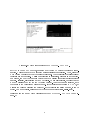
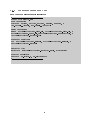
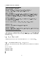
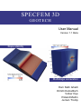
SPECFEM 3D
GEOTECH
User Manual
Version 1.1 Beta
Slope stability
Multistage excavation
Hom Nath Gharti
Dimitri Komatitsch
Volker Oye
Roland Martin
Jeroen Tromp
SPECFEM3D_GEOTECH 1.1 Beta
User Manual
1
Hom Nath Gharti , Princeton University, USA
Dimitri Komatitsch, Aix-Marseille University, France
Volker Oye, NORSAR, Norway
Roland Martin, University of Toulouse, France
Jeroen Tromp, Princeton University, USA
April 23, 2012
1 Previously
at: NORSAR, Norway
Licensing
SPECFEM3D_GEOTECH 1.1 Beta is free software: you can redistribute it and/or modify it under the terms of the GNU General Public License as published by the Free Software Foundation, either version 3 of the License, or (at your option) any later version.
SPECFEM3D_GEOTECH 1.1 Beta is distributed in the hope that it will be useful, but
WITHOUT ANY WARRANTY; without even the implied warranty of MERCHANTABILITY or FITNESS FOR A PARTICULAR PURPOSE. See the GNU General Public License for more details.
You should have received a copy of the GNU General Public License along with
SPECFEM3D_GEOTECH 1.1 Beta. If not, see <http://www.gnu.org/licenses/>.
i
Acknowledgments
This work was funded in part by the Research Council of Norway, and supported by industry partners BP, Statoil, and Total. Some of the routines were imported and modied
from the Programming the nite element method (Smith and Griths, 2004) and the
original SPECFEM3D package (e.g., Komatitsch and Vilotte, 1998; Komatitsch and
Tromp, 1999; Peter et al., 2011).
ii
Contents
Licensing
i
Acknowledgments
ii
1 Introduction
1
1.1
Background
. . . . . . . . . . . . . . . . . . . . . . . . . . . . . . . . . .
1
1.2
Status summary . . . . . . . . . . . . . . . . . . . . . . . . . . . . . . . .
2
2 Getting started
3
2.1
Package structure . . . . . . . . . . . . . . . . . . . . . . . . . . . . . . .
3
2.2
Prerequisites . . . . . . . . . . . . . . . . . . . . . . . . . . . . . . . . . .
3
2.3
Congure
2.4
Compile
2.5
Run
. . . . . . . . . . . . . . . . . . . . . . . . . . . . . . . . . . .
4
. . . . . . . . . . . . . . . . . . . . . . . . . . . . . . . . . . . .
6
. . . . . . . . . . . . . . . . . . . . . . . . . . . . . . . . . . . . . .
7
3 Input
3.1
3.2
8
Main input le
. . . . . . . . . . . . . . . . . . . . . . . . . . . . . . . .
3.1.1
Line types . . . . . . . . . . . . . . . . . . . . . . . . . . . . . . .
8
3.1.2
Arguments . . . . . . . . . . . . . . . . . . . . . . . . . . . . . . .
9
3.1.3
Examples of main input le
. . . . . . . . . . . . . . . . . . . . .
12
Input les detail . . . . . . . . . . . . . . . . . . . . . . . . . . . . . . . .
16
3.2.1
3.2.2
3.2.3
3.2.4
3.2.5
3.2.6
3.2.7
3.2.8
xfile, yfile, zfile . . . . . . . . . . . . . .
Connectivity le: confile . . . . . . . . . . . . . . . . . . . . . .
Element IDs (or Material IDs) le: idfile . . . . . . . . . . . . .
Ghost partition interfaces le: gfile . . . . . . . . . . . . . . . .
Displacement boundary conditions les: uxfile, uyfile, uzfile
Traction le: trfile . . . . . . . . . . . . . . . . . . . . . . . . .
Material list le: matfile . . . . . . . . . . . . . . . . . . . . . .
Water surface le: wsfile . . . . . . . . . . . . . . . . . . . . . .
Coordinates les:
4 Output and Visualization
4.1
4.2
8
Output les
17
18
18
18
19
20
21
23
. . . . . . . . . . . . . . . . . . . . . . . . . . . . . . . . . .
4.1.1
Summary le
4.1.2
Mesh les
4.1.3
Displacement eld le
4.1.4
Pore pressure le
4.1.5
CASE le
4.1.6
SOS le
Visualization
16
. . . . . . . . . . . . . . . . . . . . . . . . . . . . .
. . . . . . . . . . . . . . . . . . . . . . . . . . . . . . .
. . . . . . . . . . . . . . . . . . . . . . . .
23
23
23
23
. . . . . . . . . . . . . . . . . . . . . . . . . . .
23
. . . . . . . . . . . . . . . . . . . . . . . . . . . . . . .
23
. . . . . . . . . . . . . . . . . . . . . . . . . . . . . . . .
24
. . . . . . . . . . . . . . . . . . . . . . . . . . . . . . . . .
24
iii
4.2.1
Serial visualization
. . . . . . . . . . . . . . . . . . . . . . . . . .
4.2.2
Parallel visualization
. . . . . . . . . . . . . . . . . . . . . . . . .
5 Utilities
24
24
25
5.1
Convert EXODUS mesh into SEM les . . . . . . . . . . . . . . . . . . .
25
5.2
Generate SOS le . . . . . . . . . . . . . . . . . . . . . . . . . . . . . . .
25
iv
Chapter 1
Introduction
1.1 Background
SPECFEM3D_GEOTECH is a free and open-source command-driven software for 3D
slope stability analysis (for more details see Gharti et al., 2012) and simulation of 3D
multistage excavation (for more details see Gharti et al., 2012) based on the spectralelement method (e.g., Patera, 1984; Canuto et al., 1988; Seriani, 1994; Faccioli et al.,
1997; Komatitsch and Vilotte, 1998; Komatitsch and Tromp, 1999; Peter et al., 2011).
The slope stability and the excavation routines were originally started from the routines
found in the book Programming the nite element method (Smith and Griths, 2004).
The software can run on a single processor as well as multi-core machines or large clusters.
It is written mainly in FORTRAN 90, and parallelized using MPI (Gropp et al., 1994;
Pacheco, 1997) based on domain decomposition.
For the domain decomposition, the
open-source graph partitioning library SCOTCH (Pellegrini and Roman, 1996) is used.
The element-by-element preconditioned conjugate-gradient method (e.g., Hughes et al.,
1983; Law, 1986; King and Sonnad, 1987; Barragy and Carey, 1988) is implemented to
solve the linear equations. For elastoplastic failure, a Mohr-coulomb failure criterion is
used with a viscoplastic strain method
(Zienkiewicz and Cormeau, 1974).
This program does not automatically determine the factor of safety of slope stability.
Simulations can be performed for a series of safety factors.
After plotting the safety
factor verses maximum displacement curve, one can determine the factor of safety of the
given slope. Although the software is optimized for slope stability analysis and multistage
excavation, other relevant simulations of quasistatic problems in solid (geo)mechanics can
also be performed with this software.
The software currently does not include an inbuilt mesher.
Existing tools, such as
Gmsh (Geuzaine and Remacle, 2009), CUBIT (CUBIT, 2011), TrueGrid (Rainsberger,
2006), etc., can be used for hexahedral meshing, and the resulting mesh le can be
converted to the input les required by SPECFEM3D_GEOTECH. Output data can
be visualized and processed using the open-source visualization application ParaView
(www.paraview.org).
1
1.2 Status summary
Slope stability analysis
: Yes
Multistage excavation
: Yes
Gravity loading
: Yes
Surface loading
: Yes (point load, uniformly distributed load, linearly
distributed load) [Experimental]
Water table
: Yes [Experimental]
Pseudo-static earthquake loading : Yes [Experimental]
Automatic factor of safety
: No
Revisions
HNG, Jan 12, 2012; HNG, Sep 08, 2011; HNG, Jul 12, 2011; HNG, May 20, 2011; HNG,
Jan 17, 2011
2
Chapter 2
Getting started
2.1 Package structure
The original SPECFEM3D_GEOTECH package comes in a single compressed le
SPECFEM3D_GEOTECH.tar.gz,
which can be extracted using
tar
command:
tar -zxvf SPECFEM3D_GEOTECH.tar.gz
or using, for example,
7-zip (www.7-zip.org) under WINDOWS. The package has the
following structure:
SPECFEM3D_GEOTECH/
COPYING
: License.
README
: brief description of the package.
CMakeLists.txt
: CMake conguration le.
bin/
: all object les and executables are stored in this folder.
doc/
: documentation les for the SPECFEM3D_GEOTECH package. If
built this le is created.
input/
: contains input les.
partition/
: contains partition les for parallel processing.
output/
:
default output folder.
All output les are stored in this folder
unless the dierent output path is dened in the main input le.
src/
: contains all source les.
2.2 Prerequisites
≥ 2.8.4 is necessary to congure the software.
downloaded from www.cmake.org.
- CMake build system. The CMake version
It is free and open-source, and can be
3
- Make utility. The make utility is necessary to build the software using Makele. This
utility is usually installed by default in most LINUX systems. Under WINDOWS, one
can use Cygwin (www.cygwin.com) or MinGW (www.mingw.org) to install the make
utility.
- A recent FORTRAN compiler. The software is written mainly in FORTRAN 90, but
it also uses a few FORTRAN 2003 features (e.g., streaming IO). These features are
already available in most of the FORTRAN compilers, e.g., gfortran version
≥
4.2
(gcc.gnu.org/wiki/GFortran) and g95 (www.g95.org).
Following libraries are necessary for parallel processing.
- A recent MPI library. It should be built with the same FORTRAN compiler used to
compile
the
software.
Please
www.mcs.anl.gov/research/projects/mpich2
www.open-mpi.org
see
or
for details on how to install MPI li-
brary and how to run MPI programs.
- SCOTCH graph partitioning library. This library should be compiled with the same
FORTRAN
compiler
used
to
compile
www.labri.fr/perso/pelegrin/scotch
the
software.
Please
see
for details on how to install SCOTCH.
Finally, the following compiler is necessary to build the documentation (this le):
AT X compiler. This is necessary to compile the documentation les.
- L
E
2.3 Congure
Software package SPECFEM3D_GEOTECH is congured using CMake, and the package
uses an out-of-source build. Hence, DO NOT build in the same source directory. Let's say
the full path to the package (source directory) is
ˆ
Create a separate build directory, e.g.,
ˆ
Go to the build directory
ˆ
Type the cmake command
$HOME/download/SPECFEM3D_GEOTECH.
mkdir $HOME/work/SPECFEM3D_GEOTECH
cd $HOME/work/SPECFEM3D_GEOTECH
ccmake $HOME/projects/SPECFEM3D_GEOTECH
CMake conguration is an iterative process (See Figure 2.1):
ˆ
Congure (c key or Congure button)
ˆ
Change variables' values if necessary
ˆ
Congure (c key or Congure button)
4
Figure 2.1: CMake conguration of SPECFEM3D_GEOTECH .
If WARNINGS or ERRORS occur, press the e key (or the OK button) to return to conguration. These steps have to be repeated until successful conguration. Then, press the
g key (or the Generate button) to generate build les. Check carefully that all necessary
variables are set properly.
Unless conguration is successful, generate is not enabled.
Sometimes, the c key (or Congure button) has to be pressed repeatedly until generate is
enabled. Initially, all variables may not be visible. To see all variables, toggle advanced
mode by pressing the t key (or the Advanced button). To set or change a variable, move
the cursor to the variable and press Enter key. If the variable is a boolean (ON/OFF), it
will ip the value on pressing the Enter key. If the variable is a string or a le, it can be
edited. For more details, please see the CMake documentation (www.cmake.org).
Following are the main CMake variables for the SPECFEM3D_GEOTECH (See Figure 2.1)
5
BUILD_DOCUMENTATION
:
If
ON,
the user manual (this le) is created.
BUILD_PARTMESH
The
OFF.
default is
ON, the partmesh program is built. The default is
OFF. The partmesh program is necessary to partition
: If
the mesh for parallel processing.
BUILD_UTILITIES_EXODUS2SEM
:
ON,
If
exodus
exodus2sem program is built. The
OFF. The exodus2sem program convert
the
default is
mesh
le
to
input
les
required
by
the
SPECFEM3D_GEOTECH package (see also Chapter 5).
BUILD_UTILITIES_WRITE_SOS
ON, the write_sos program is built. The default
is OFF. The write_sos program writes a EnSight SOS
: If
le necessary for the parallel visualization (see also
Chapter 5).
ENABLE_MPI
:
If
ON,
built otherwise main serial
built. The default is
SCOTCH_LIBRARY_PATH
:
psemgeotech
program semgeotech
the main parallel program
OFF.
This is required if
BUILD_PARTMESH
is
ON.
is
is
If not
found automatically, it can be set manually.
CMAKE_Fortran_COMPILER
: This denes the Fortran compiler. If not found automatically or the automatically found compiler is not
correct, it can be set manually.
Note 1: If CMAKE_Fortran_COMPILER has to be changed, rst change this and congure,
and then change other variables if necessary and congure.
Note 2: Even if some of the above variables are set ON, if appropriate working compilers
are not found, corresponding variables are internally set OFF with WARNING messages.
2.4 Compile
Once conguration and generation are successful, the necessary build les are created.
Now to build the main program, type:
make
On multi-processor systems (let's say eight processors), type:
make -j 8
To clean, type
make clean
Note: If reconguration is necessary, it is better to delete all Cache les of the build
directory.
6
2.5 Run
Serial run
- To run the serial program, type
./bin/semgeotech input_le_name
Example:
./bin/semgeotech ./input/validation1.sem
Parallel run
- To partition the mesh, type
./bin/partmesh input_le_name
Example:
./bin/partmesh ./input/validation1.psem
- To run the parallel program, type
mpirun -n number_of_nodes ./bin/psemgeotech input_le_name
OR
mpirun -n number_of_nodes --hostfile host_le ./bin/psemgeotech input_le_name
Example:
mpirun -n 8 ./bin/psemgeotech ./input/validation1.psem
Note: see Chapter 3 for details on input and input les. Try to run one or more examples
included in input/. By default, example les included in the package are not copied to
build directory during build process. If necessary, copy les within input/ folder of source
directory to the input/ folder of build directory.
7
Chapter 3
Input
3.1 Main input le
The main input le structure is motivated by the E3D (Larsen and Schultz, 1995)
software package.
The main input le consists of legitimate input lines dened in the
specied formats. Any number of blank lines or comment lines can be placed for user
friendly input structure. The blank lines contain no or only white-space characters, and
the comment lines contain "#" as the rst character.
Each legitimate input line consists of a line type, and list of arguments and corresponding
values. All argument-value pair are separated by comma (,). If necessary, any legitimate
input line can be continued to next line using FORTRAN 90 continuation character "&"
as an absolute last character of a line to be continued. Repetition of same line type is
not allowed.
Legitimate input lines have the format
line_type arg1 = val1 , arg2 = val2 ,
.......,
argn = valn
Example:
preinfo: nproc=8, ngllx=3, nglly=3, ngllz=3, nenod=8, ngnod=8, &
inp_path='../input', part_path='../partition', out_path='../output/'
All legitimate input lines should be written in lower case. Line type and argument-value
pairs must be separated by a space. Each argument-value pair must be separated by a
comma(,) and a space/s. No space/s are recommended before line type and in between
argument name and "=" or "=" and argument value. If argument value is a string, the
FORTRAN 90 string (i.e., enclosed within single quotes) should be used, for example,
inp_path='../input'.
If the argument value is a vector (i.e., multi-valued), a list of
values separated by space (no comma!) shoud be used, e.g,
3.1.1 Line types
Only the following line types are permitted.
preinfo:
preliminary information of the simulation
mesh:
mesh information
8
srf=1.0 1.2 1.3 1.4.
bc:
boundary conditions information
traction:
traction information [optional]
stress0:
initial stress information [optional]. It is generally necessary for multistage
excavation.
material:
material properties
eqload:
pseudo-static earthquake loading [optional]
water:
water table information [optional]
control:
control of the simulation
save:
options to save data
3.1.2 Arguments
Only the following arguments under the specied line types are permitted.
preinfo:
nproc
: number of processors to be used for the parallel processing [integer > 1].
Only required for parallel processing.
ngllx
: number of Gauss-Lobatto-Legendre (GLL) points along
x-axis
[integer >
1].
nglly
: number of GLL points along
y -axis
[integer > 1].
ngllz
: number of GLL points along
z -axis
[integer > 1].
Note: Although the program can use dierent values of ngllx, nglly, and
ngllz, it is recommended to use same number of GLL points along all axes.
inp_path
: input path where the input data are located [string, optional, default
part_path
: partition path where the partitioned data will be or are located [string,
optional, default
out_path
⇒
'../input'].
⇒ '../partition'].
Only required for parallel processing.
: output path where the output data will be stored [string, optional, default
⇒ '../output'].
mesh:
xfile
: le name of
x-coordinates
[string].
yfile
: le name of
y -coordinates
[string].
zfile
: le name of
z -coordinates
[string].
9
confile
: le name of mesh connectivity [string].
idfile
: le name of element IDs [string].
gfile
: le name of ghost interfaces, i.e., partition interfaces [string].
Only re-
quired for parallel processing.
bc:
uxfile
: le name of displacement boundary conditions along
x-axis
[string].
uyfile
: le name of displacement boundary conditions along
y -axis
[string].
uzfile
: le name of displacement boundary conditions along
z -axis
[string].
traction:
trfile
: le name of traction specication [string].
stress0:
type
: type of initial stress [integer, optional, 0 = compute using SEM itself, 1 =
compute using simple vertical lithostatic relation, default
⇒
0].
z0
: datum (free surface) coordinate [real, m]. Only required if
s0
: datum (free surface) vertical stress [real, kN/m ]. Only required if
k0
: lateral earth pressure coecient [real].
2
type=1.
type=1.
material:
matfile
: le name of material list [string].
ispart
: ag to indicate whether the material le is partitioned [integer, optional,
0 = No, 1 = Yes, default
matpath
⇒
1]. Only required for parallel processing.
⇒ '../input' for serial or
'../partition' for partitioned
: path to material le [string, optional, default
unpartitioned material le in parallel and
material le in parallel].
allelastic
: assume all entire domain as elastic [integer, optional, 0 = No, 1 = Yes,
default
⇒
0].
eqload:
eqkx
: pseudo-static earthquake loading coecient along
<= 1.0, default
eqky
⇒
: pseudo-static earthquake loading coecient along
<= 1.0, default
⇒
x-axis
[real, 0 <=
eqkx
y -axis
[real, 0 <=
eqky
0.0].
0.0].
10
eqkz
: pseudo-static earthquake loading coecient along
<= 1.0, default
⇒
z -axis
[real, 0 <=
eqkz
0.0].
Note: For the stability analysis purpose, these coecients should be chosen carefully. For example, if the slope face is pointing towards the negative
x-axis, value of eqkx is taken negative.
water:
wsfile
: le name of water surface le.
control:
cg_tol
: tolerance for conjugate gradient method [real].
cg_maxiter
: maximum iterations for conjugate gradient method [integer > 0].
nl_tol
: tolerance for nonlinear iterations [real].
nl_maxiter
: maximum iterations for nonlinear iterations [integer > 0].
ninc
: number of load increments for the plastic iterations [integer>0 default
⇒
1].This is currently not used for slope stability analysis.
Arguments specific to slope stability analysis:
nsrf
: number of strength reduction factors to try [integer > 0, optional, default
⇒
srf
1].
: values of strength reduction factors [real vector, optional, default
Number of
phinu
: force
srfs
φ−ν
must be equal to
⇒
1.0].
nsrf.
(Friction angle - Poisson's ratio) inequality:
(see Zheng et al., 2005) [integer, 0 = No, 1 = Yes, default
sin φ ≥ 1 − 2 ν
⇒ 0]. Only for
TESTING purpose.
Arguments specific to multistage excavation:
nexcav
: number of excavation stages [integer > 0, optional, default
nexcavid
: number of excavation IDs in each excavation stage [integer vector, default
⇒
excavid
⇒
1].
1].
: IDs of blocks/regions in the mesh to be excavated in each stage [integer
vector, default
⇒
1].
Note: Do not mix arguments for slope stability and excavation.
save:
disp
: displacement eld [integer, optional, 0 = No, 1 = Yes, default
porep
: pore water pressure [integer, optional, 0 = No, 1 = Yes, default
11
⇒
0].
⇒
0].
3.1.3 Examples of main input le
Input le for a simple elastic simulation
##input file elastic.sem
#pre information
preinfo: ngllx=3, nglly=3, ngllz=3, nenod=8, ngnod=8, &
inp_path='../input', out_path='../output/'
#mesh information
mesh: xfile='validation1_coord_x', yfile='validation1_coord_y', &
zfile='validation1_coord_z', confile='validation1_connectivity', &
idfile='validation1_material_id'
#boundary conditions
bc: uxfile='validation1_ssbcux', uyfile='validation1_ssbcuy', &
uzfile='validation1_ssbcuz'
#material list
material: matfile='validation1_material_list', allelastic=1
#control parameters
control: cg_tol=1e-8, cg_maxiter=5000
#-
12
Serial input le for slope stability
##input file validation1.sem
#pre information
preinfo: ngllx=3, nglly=3, ngllz=3, nenod=8, ngnod=8, &
inp_path='../input', out_path='../output/'
#mesh information
mesh: xfile='validation1_coord_x', yfile='validation1_coord_y', &
zfile='validation1_coord_z', confile='validation1_connectivity', &
idfile='validation1_material_id'
#boundary conditions
bc: uxfile='validation1_ssbcux', uyfile='validation1_ssbcuy', &
uzfile='validation1_ssbcuz'
#material list
material: matfile='validation1_material_list'
#control parameters
control: cg_tol=1e-8, cg_maxiter=5000, nl_tol=0.0005, nl_maxiter=3000, &
nsrf=9, srf=1.0 1.5 2.0 2.15 2.16 2.17 2.18 2.19 2.20
#-
13
Parallel input le for slope stability
##input file validation1.psem
#pre information
preinfo: nproc=8, ngllx=3, nglly=3, ngllz=3, nenod=8, &
ngnod=8, inp_path='../input', out_path='../output/'
#mesh information
mesh: xfile='validation1_coord_x', yfile='validation1_coord_y', &
zfile='validation1_coord_z', confile='validation1_connectivity', &
idfile='validation1_material_id', gfile='validation1_ghost'
#boundary conditions
bc: uxfile='validation1_ssbcux', uyfile='validation1_ssbcuy', &
uzfile='validation1_ssbcuz'
#material list
material: matfile='validation1_material_list'
#control parameters
control: cg_tol=1e-8, cg_maxiter=5000, nl_tol=0.0005, nl_maxiter=3000, &
nsrf=9, srf=1.0 1.5 2.0 2.15 2.16 2.17 2.18 2.19 2.20
#-
14
Serial input le for excavation
##input file excavation_3d.sem
#pre information
preinfo: ngllx=3, nglly=3, ngllz=3, nenod=8, ngnod=8, &
inp_path='../input', out_path='../output/'
#mesh information
mesh: xfile='excavation_3d_coord_x', yfile='excavation_3d_coord_y', &
zfile='excavation_3d_coord_z', confile='excavation_3d_connectivity', &
idfile='excavation_3d_material_id'
#boundary conditions
bc: uxfile='excavation_3d_ssbcux', uyfile='excavation_3d_ssbcuy', &
uzfile='excavation_3d_ssbcuz'
#initial stress stress0:
type=0, z0=0, s0=0, k0=0.5, usek0=1
#material list
material: matfile='excavation_3d_material_list'
#control parameters
control: cg_tol=1e-8, cg_maxiter=5000, nl_tol=0.0005, nl_maxiter=3000, &
nexcav=3, excavid=2 3 4, ninc=10
#-
15
Parallel input le for excavation
##input file excavation_3d.psem
#pre information
preinfo: nproc=8, ngllx=3, nglly=3, ngllz=3, nenod=8, &
ngnod=8, inp_path='../input', out_path='../output/'
#mesh information
mesh: xfile='excavation_3d_coord_x', yfile='excavation_3d_coord_y', &
zfile='excavation_3d_coord_z', confile='excavation_3d_connectivity', &
idfile='excavation_3d_material_id', gfile='excavation_3d_ghost'
#boundary conditions
bc: uxfile='excavation_3d_ssbcux', uyfile='excavation_3d_ssbcuy', &
uzfile='excavation_3d_ssbcuz'
#initial stress stress0:
type=0, z0=0, s0=0, k0=0.5, usek0=1
#material list
material: matfile='excavation_3d_material_list'
#control parameters
control: cg_tol=1e-8, cg_maxiter=5000, nl_tol=0.0005, nl_maxiter=3000, &
nexcav=3, excavid=2 3 4, ninc=10
#'nproc'
'mesh' in
There are only two additional pieces of information, i.e., number of processors
in line
'preinfo'
and le name for ghost partition interfaces
'gfile'
in line
parallel input le.
3.2 Input les detail
All local element/face/edge/node numbering follows the EXODUS II convention.
3.2.1 Coordinates les: xfile, yfile, zfile
Each of the coordinates les contains a list of corresponding coordinates in the following
format:
number of
coordinate
coordinate
coordinate
..
..
points
of point 1
of point 2
of point 3
16
..
Example:
2354
40.230394465164999
40.759090909090901
42.700000000000003
40.957142857142898
40.230394465164999
40.759090909090901
42.700000000000003
40.957142857142898
...
...
3.2.2 Connectivity le: confile
The connectivity le contains the connectivity lists of elements in the following format:
number of elements
n1 n2 n3 n4 n5 n6 n7
n1 n2 n3 n4 n5 n6 n7
n1 n2 n3 n4 n5 n6 n7
n1 n2 n3 n4 n5 n6 n7
..
..
n8
n8
n8
n8
of
of
of
of
element
element
element
element
1
2
3
4
Example:
1800
1 2 3 4 5 6 7 8
9 10 2 1 11 12 6 5
9 1 4 13 11 5 8 14
15 16 10 9 17 18 12 11
15 9 13 19 17 11 14 20
21 22 16 15 23 24 18 17
21 15 19 25 23 17 20 26
27 28 22 21 29 30 24 23
27 21 25 31 29 23 26 32
33 34 28 27 35 36 30 29
33 27 31 37 35 29 32 38
34 33 39 40 36 35 41 42
33 37 43 39 35 38 44 41
...
...
17
3.2.3 Element IDs (or Material IDs) le: idfile
This le contains the IDs of elements. This ID will be used in the program mainly to
identify the material regions. This le has the following format:
number of elements
ID of element 1
ID of element 2
ID of element 3
ID of element 4
...
...
Example:
1800
1
1
1
1
1
1
1
1
1
1
...
...
3.2.4 Ghost partition interfaces le: gfile
This le will be generated automatically by a program
partmesh.
3.2.5 Displacement boundary conditions les: uxfile, uyfile,
uzfile
This le contains information on the displacement boundary conditions (currently only
the zero-displacement is implemented), and has the following format:
number of element faces
elementID faceID
elementID faceID
elementID faceID
...
...
18
Example:
849
2 2
3 4
5 1
6 1
7 1
8 1
9 1
...
...
3.2.6 Traction le: trfile
This le contains the traction information on the model in the following format:
traction type (integer, 0 = point, 1 = uniformly distributed, 2 = linearly
if traction type = 0
qx qy qz (load vector in kN)
if traction type = 1
qx qy qz (load vector in kN/m2 )
if traction type = 2
relevant-axis x1 x2 qx1 qy1 qz1 qx2 qy2 qz2
number of entities (points for point load or faces for distributed load)
elementID entityID
elementID entityID
elementID entityID
...
...
distributed)
This can be repeated as many times as there are tractions.
The
relevant-axis
denotes the axis along which the load is varying, and is represented by
x-axis, 2 = y -axis, and 3 = z -axis. The variables x1 and x2 denote the
relevant-axis ) of two points between which the linearly distributed
Similarly, qx1 , qy1 and qz1 , and qx2 , qy2 and qz2 denote the load vectors in
an integer as 1 =
coordinates (only the
load is applied.
kN/m
2
at the point 1 and 2, respectively.
Example:
The following data specify the two tractions: a uniformly distributed traction and a linearly distributed traction.
1
0.0 0.0 -167.751
363
19
56 1
57 1
58 1
59 1
60 1
61 1
62 1
...
...
2
3 7.3 24.4 51.8379 0.0 -159.5407 0.0 0.0 0.0
594
38 1
39 1
40 1
41 1
42 1
43 1
44 1
45 1
46 1
...
...
3.2.7 Material list le: matfile
This le contains material properties of each material regions. Material properties must
be listed in a sequential order of the unique material IDs.
In addition, this data le
optionally contains the information on the water condition of material regions. Material
regions or material IDs must be consistent with the Material IDs (Element IDs) dened
in
idfile.
The
matfile
has the following format:
comment line
number of material regions (unique material IDs)
materialID, domainID, γ , E , ν , φ, c, ψ
materialID, domainID, γ , E , ν , φ, c, ψ
materialID, domainID, γ , E , ν , φ, c, ψ
...
...
number of submerged material regions
submerged materialID
submerged materialID
...
...
The
materilID
must be in a sequential order starting from 1. The
20
doaminID
represents
the material domain (e.g., isotropic or anisotropic), and it is currently irrelevant, therefore, always use 1.
modulus of elasticity in
2
in kN/m , and
ψ
γ represents the unit weight in kN/m3 , E
2
kN/m , φ the angle of internal friction in degrees, c
Similarly,
the Young's
the cohesion
the angle of dilation in degrees.
Example:
The following data denes four material regions. No region is submerged in water.
#
4
1
2
3
4
material properties (id, domain, gamma, ym, nu, phi, coh, psi)
1
1
1
1
18.8
19.0
18.1
18.5
1e5
1e5
1e5
1e5
0.3
0.3
0.3
0.3
20.0
20.0
20.0
20.0
29.0
27.0
20.0
29.0
0.0
0.0
0.0
0.0
The following data denes four material regions with two of them submerged.
#
4
1
2
3
4
2
1
3
material properties (id, domain, gamma, ym, nu, phi, coh, psi)
1
1
1
1
18.8
19.0
18.1
18.5
1e5
1e5
1e5
1e5
0.3
0.3
0.3
0.3
20.0
20.0
20.0
20.0
0.0 0.0
27.0 0.0
0.0 0.0
29.0 0.0
3.2.8 Water surface le: wsfile
This le contains the water table information on the model in the format as
number of water surfaces
water surface type (integer,
0 = horizontal surface, 1 = inclined surface, 2 = meshed
surface)
wstype =0 (can be reconstructed by sweeping a horizontal line)
relevant-axis x1 x2 z
if wstype =1 (can be reconstructed by sweeping a inclined line)
relevant-axis x1 x2 z1 z2
if wstype =2 (meshed surface attached to the model)
number of faces
elelemetID, faceID
elelemetID, faceID
elelemetID, faceID
...
...
if
21
relevant-axis denotes the axis along which the line is dened, and it is taken as 1 =
x-axis, 2 = y -axis, and 3 = z -axis. The variables x1 and x2 denote the coordinates (only
relevant-axis ) of point 1 and 2 that dene the line. Similarly, z denotes a z -coordinate
of a horizontal water surface, and z1 and z2 denote the z -coordinates of the two points
The
(that dene the line) on the water surface.
Example:
Following data specify the two water surfaces: a horizontal surface and an inclined surface.
2
0
1 42.7 50.0 6.1
1
1 0.0 42.7 12.2 6.1
22
Chapter 4
Output and Visualization
4.1 Output les
4.1.1 Summary le
This le is self explanatory and it contains a summary of the results including control
parameters, maximum displacement at each step, and elapsed time. The le is written
input_le_name_header _summary
input_le_name_header _summary_procprocessor_ID for parallel run.
in ASCII format and its name follows the convention
for serial run and
4.1.2 Mesh les
This le contains the mesh information of the model including coordinates, connectivity, element types, etc., in EnSight Gold binary format (see EnSight, 2008).
input_le_name_header _summary for
put_le_name_header _summary_procprocessor_ID for parallel run.
le name follows the format
The
serial run and
in-
4.1.3 Displacement eld le
This le contains the nodal displacement eld in the model written in EnSight Gold
input_le_name_header _stepstep .dis
input_le_name_header _stepstep _procprocessor_ID .dis for parallel
binary format. The le name follows the format
for serial run and
runs.
4.1.4 Pore pressure le
This le contains the hydrostatic pore pressure eld in the model written in EnSight Gold
input_le_name_header _stepstep .por
input_le_name_header _stepstep _procprocessor_ID .por for parallel
binary format. The le name follows the format
for serial run and
run.
4.1.5 CASE le
This is an EnSight Gold CASE le written in ASCII format. This le contain the in-
input_le_name_header .case for serial run and input_le_name_header _procprocessor_ID .case
formation on the mesh les, other les, time steps etc. The le name follows the format
for parallel run.
23
4.1.6 SOS le
This is an EnSight Gold server-of-server le for parallel visualization. The
/utilities/
program provided in the
write_sos.f90
may be used to generate this le. See Chapter 5,
Section 5.2 for more detail.
All above EnSight Gold les correspond to the model with spectral-element mesh. Additionally, the CASE le/s and mesh le/s are written for the original model. These le
names follow the similar conventions and they have the tag
'original'
in the le name
headers.
4.2 Visualization
4.2.1 Serial visualization
Requirement: ParaView version later than 3.7. Precompiled binaries available from ParaView web (www.paraview.org) may be installed directly or it can be build from the
source.
ˆ
open a session
ˆ
open paraview client
ˆ
paraview
In ParaView client:
⇒
File
⇒
Open
select appropriate serial CASE le (.case le)
see ParaView wiki
paraview.org/Wiki/ParaView
for more detail.
4.2.2 Parallel visualization
Requirement:
ParaView version later than 3.7.
It should be built enabling MPI. An
appropriate MPI library is necessary.
ˆ
open a session
ˆ
open paraview client
ˆ
start ParaView server
paraview
mpirun -np 8 pvserver -display :0
ˆ
In ParaView client:
⇒
File
ˆ
In ParaView client:
⇒
Open
⇒
Connect and connect to the appropriate server
select appropriate SOS le (.sos le)
see ParaView wiki (paraview.org/Wiki/ParaView for more detail.
Note: Each CASE le obtained from the parallel processing can also be visualized in a
serial.
24
Chapter 5
Utilities
5.1 Convert EXODUS mesh into SEM les
The program
exodus2sem.c contained in the utilities directory can be used to convert the
mesh le in EXODUS II format to input les required by the SPECFEM3D_GEOTECH
.
Compile
gcc -o exodus2sem exodus2sem.c
Run
exodus2sem EXODUS_mesh_le OPTIONS
For more details, see /utilities/README_exodus2sem.
It can also be compiled au-
tomatically during the build process of main package SPECFEM3D_GEOTECH (see
Section 2.3).
5.2 Generate SOS le
The program
write_sos.f90
contained in the utilities directory can be used to write
EnSight Gold server-of-server le (.sos le, see (EnSight, 2008)) to visualize the multiprocessors data in parallel. This le does not contain the actual data, but only information
on the data location and parallel processing.
Compile
gfortran -o write_sos write_sos.f90
Run
exodus2sem input_le
For more details, see
/utilities/README_write_sos.
It can also be compiled auto-
matically during the build process of main package SPECFEM3D_GEOTECH (see Section 2.3).
25
Bibliography
Barragy, E. and G. F. Carey (1988).
A parallel element-by-element solution scheme.
International Journal for Numerical Methods in Engineering 26,
23672382.
Canuto, C., M. Y. Hussaini, A. Quarteroni, and T. A. Zang (1988).
uid dynamics.
CUBIT (2011).
Spectral methods in
Springer.
CUBIT 13.0 User Documentation. Sandia National Laboratories. [Online;
accessed 27-May-2011].
EnSight (2008).
EnSight User Manual
(Version 9.0 ed.). Salem Street, Suite 101, Apex,
NC 27523 USA: Computational Engineering International, Inc. [Online; accessed 11July-2011].
Faccioli, E., F. Maggio, R. Paolucci, and A. Quarteroni (1997).
2D and 3D elastic
wave propagation by a pseudo-spectral domain decomposition method.
Seismology 1,
Journal of
237251.
Geuzaine, C. and J. F. Remacle (2009). Gmsh: a three-dimensional nite element mesh
generator with built-in pre- and post-processing facilities.
Numerical Methods in Engineering 79 (11),
International Journal for
13091331.
Gharti, H. N., D. Komatitsch, V. Oye, R. Martin, and J. Tromp (2012). Application of
an elastoplastic spectral-element method to 3D slope stability analysis.
Journal for Numerical Methods in Engineering in press.
International
Gharti, H. N., V. Oye, D. Komatitsch, and J. Tromp (2012). Simulation of multistage
excavation based on a 3d spectral-element method.
Computers & Structures 100101,
5469.
Gropp, W., E. Lusk, and A. Skjellum (1994).
with the Message-Passing Interface.
Using MPI, portable parallel programming
Cambridge, USA: MIT Press.
Hughes, T. J. R., I. Levit, and J. Winget (1983). An element-by-element solution algorithm for problems of structural and solid mechanics.
Mechanics and Engineering 36 (2),
Computer Methods in Applied
241254.
King, R. B. and V. Sonnad (1987). Implementation of an element-by-element solution algorithm for the nite element method on a coarse-grained parallel computer.
Methods in Applied Mechanics and Engineering 65 (1),
Computer
4759.
Komatitsch, D. and J. Tromp (1999). Introduction to the spectral element method for
three-dimensional seismic wave propagation.
806822.
26
Geophysical Journal International 139,
Komatitsch, D. and J. P. Vilotte (1998). The spectral element method: An ecient tool
Bulletin of the
to simulate the seismic response of 2D and 3D geological structures.
Seismological Society of America 88 (2),
Larsen, S. and C. A. Schultz (1995).
368392.
ELAS3D: 2D/3D elastic nite dierence wave
propagation code: Technical Report No. UCRL-MA-121792. Technical report.
Law, K. H. (1986).
tures 23 (6),
A parallel nite element solution method.
Computers & Struc-
845858.
Pacheco, P. (1997).
Parallel Programming with MPI.
Morgan Kaufmann.
Patera, A. T. (1984). A spectral element method for uid dynamics: laminar ow in a
channel expansion.
Journal of Computational Physics 54,
468488.
Pellegrini, F. and J. Roman (1996). SCOTCH: A software package for static mapping
by dual recursive bipartitioning of process and architecture graphs.
Computer Science 1067,
Lecture Notes in
493498.
Peter, D., D. Komatitsch, Y. Luo, R. Martin, N. Le Go, E. Casarotti, P. Le Loher,
F. Magnoni, Q. Liu, C. Blitz, T. Nissen-Meyer, P. Basini, and J. Tromp (2011). Forward
and adjoint simulations of seismic wave propagation on fully unstructured hexahedral
meshes.
Geophysical Journal International 186 (2),
Rainsberger, R. (2006).
TrueGrid User's Manual
721739.
(version 2.3.0 ed.).
Livermore, CA:
XYZ Scientic Applications, Inc.
Seriani, G. (1994). 3-D large-scale wave propagation modeling by spectral element method
on Cray T3E multiprocessor.
ing 164,
Computer Methods in Applied Mechanics and Engineer-
235247.
Smith, I. M. and D. V. Griths (2004).
Programming the nite element method.
John
Wiley & Sons.
Zheng, H., D. F. Liu, and C. G. Li (2005). Slope stability analysis based on elasto-plastic
nite element method.
International Journal for Numerical Methods in Engineering 64,
18711888.
Zienkiewicz, O. and I. Cormeau (1974). Visco-plasticityplasticity and creep in elastic
solids a unied numerical solution approach.
Methods in Engineering 8 (4),
821845.
27
International Journal for Numerical