1
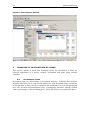
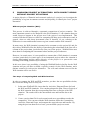
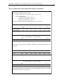
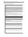
WinDASI: A Software for Cost Benefit Analysis of Investment Projects Calculations Performed by the Software Module 020 WinDASI: A Software for Cost Benefit Analysis of Investment Projects Calculations Performed by the Software WinDASI: A Software for Cost Benefit Analysis of Investment Projects Calculations Performed by the Software by Lorenzo Giovanni Bellù, Agricultural Policy Support Service, Policy Assistance Division, Food and Agriculture Organization of the United Nations, FAO, Rome, Italy for the Food and Agriculture Organization of the United Nations, FAO About EASYPol EASYPol is a an on-line, interactive multilingual repository of downloadable resource materials for capacity development in policy making for food, agriculture and rural development. The EASYPol home page is available at: www.fao.org/tc/easypol. EASYPol has been developed and is maintained by the Agricultural Policy Support Service, FAO. The designations employed and the presentation of the material in this information product do not imply the expression of any opinion whatsoever on the part of the Food and Agriculture Organization of the United Nations concerning the legal status of any country, territory, city or area or of its authorities, or concerning the delimitation of its frontiers or boundaries. © FAO November 2005: All rights reserved. Reproduction and dissemination of material contained on FAO's Web site for educational or other non-commercial purposes are authorized without any prior written permission from the copyright holders provided the source is fully acknowledged. Reproduction of material for resale or other commercial purposes is prohibited without the written permission of the copyright holders. Applications for such permission should be addressed to: [email protected]. WinDASI: A Software for Cost Benefit Analysis of Investment Projects Calculations Performed by the Software Acknowledgements This module draws upon the TCAS publication: WinDASI User Manual, Training Materials for Agricultural Planning, 43 FAO - Rome 2000, whose main contributors are Carlo Cappi, who is also the main designer of the computer software, and Lorenzo Giovanni Bellù. The author would like to acknowledge with thanks the contribution of Francesca Petrina, who volunteered for reviewing the first draft of this module and to all the others who contributed in different ways to this final version. The WinDASI software was developed by Laurent Cazalet and Gilles Cappella under the supervision of Mahmoud Allaya at the “Institut Agonomique Méditerraneén de Montpellier (IAM-M)-France. WinDASI: A Software for Cost Benefit Analysis of Investment Projects Calculations Performed by the Software Table of contents 1 Summary ...................................................................................1 2 Introduction................................................................................1 3 Steps to carry out calculations of flows and indicators.......................2 3.1 Step 1: Get the “calculation options” window.................................... 2 3.2 Step 2: Select the type of calculation you wish to carry out ................ 2 3.3 Step 3: Calculate flows of quantities and costs/benefits...................... 3 3.4 Step 4: Calculate indicators ........................................................... 6 3.5 Step 5: Run Sensitivity tests and comparisons ................................ 10 4 Examples of calculations of flows ................................................. 14 4.1 Investment items ........................................................................ 14 4.2 Plans ......................................................................................... 16 5 Comparing project alternatives: with-project versus without-project situations ................................................................................. 19 6 Normal versus phased modes of calculation................................... 20 7 Conclusions .............................................................................. 24 8 Readers’ notes .......................................................................... 24 8.1 EASYPol links ............................................................................. 24 Module metadata.............................................................................. 26 WinDASI: a Software for Cost Benefit Analysis of Investment Projects Calculations Performed by the Software 1 1 SUMMARY This module illustrates how to carry out cost-benefit calculations of investment projects in WinDASI, after data are inserted in the database. It explains, by means of a step-by step procedure, how to calculate: a) flows of physical quantities of outputs, inputs and investment items; b) flows of current, discounted and cumulative costs, benefits, and net benefits; c) flows of incremental (With-Without project) current, discounted and cumulative net benefits; and e) project indicators such as the Net Present Value (NPV), the Internal Rate of Return (IRR), the Benefit/Cost Ratio, (BCR), the Switching Values (SVs) and Sensitivity Analysis. Instructions are provided on how to carry out calculations for the different components of an investment project, notably: plans, zones and projects (i.e. at different levels of aggregation). In addition, this module addresses normal and phased mode of calculation and comparisons of different projects alternative scenarios (with–project versus without-project). 2 INTRODUCTION Objectives The main objective of this module is to illustrate how to carry out Cost-Benefit calculations in WinDASI after having inserted project data in the data-base. To this end, the user is driven by means of step-by-step procedures to calculate flows of costs and benefits and main project indicators. After reading this document, to be used in parallel with the software, the user will be able to handle WinDASI to perform the analysis of financial and economic viability of investment projects. Target audience This module targets current or future practitioners in Cost-Benefit Analysis (CBA) of investment projects, working in public administrations, in NGO’s, professional organizations or consulting firms. Also academics can find this material useful to support their courses in CBA and development economics. Furthermore, students can use this material to improve their skills in CBA and complement their curricula. Required background To fully understand the content of this module the user must be familiar with: concepts of project cycle management; concepts of project financial analysis; concepts of project economic analysis. The insertion and management of project data in WinDASI. 2 EASYPol Module 020 Analytical Tools Selected EASYPol modules can be used to strengthen the background of the reader and to further expand its knowledge about investment projects and cost-benefit analysis. Links with relevant EASYPol modules, further readings and references are reported both in the text and in the last section of the module1. 3 STEPS TO CARRY OUT CALCULATIONS OF FLOWS AND INDICATORS Before starting the calculations, the user must have inserted relevant data in the database2. Once data are inserted, Cost-Benefit calculations in WinDASI are carried out in five main steps, as follows: Step 1: get the “calculation options” window. Step 2: select the type of calculation you wish to carry out Step 3: calculate of flows of physical quantities and costs/benefits Step 4: calculate indicators. Step 5: run Sensitivity tests and comparisons. These steps are described here below and examples are provided in the next section. 3.1 Step 1: Get the “calculation options” window There are two ways to get the “calculation options” window: i. ii. either click on the Calculation button on the Main Toolbar; then choose the component for which you wish to carry out the calculation: Plan, Zone or Project, or click on the Calculation button in the window of a Plan, Zone or a Project. In either case, the “Calculation options” window (Figure 1) will pop up. 3.2 Step 2: Select the type of calculation you wish to carry out Select the calculation option you wish to carry out from amongst the list of calculation options (see Figure 1): whether the calculation should be carried out either for inputs or outputs, “by quantity” or “by value” If the calculations are to be carried out “by value”, 1 EASYPol hyperlinks are shown in blue, as follows: a) training paths are shown in underlined bold font; b) other EASYPol modules or complementary EASYPol materials are in bold underlined c) links to the glossary are in bold; and d) external links are in italics. 2 italics; The EASYPol Module 019: WinDASI-A Software for Cost-Benefit Analysis of Investment Projects : Inserting and Managing Data provides guidance on how to load project data into WinDASI. WinDASI: a Software for Cost Benefit Analysis of Investment Projects Calculations Performed by the Software 3 you will have also to specify whether to use “Financial prices” or “Economic prices3”. If the “by Value” option is chosen also the Net Benefit flows can be calculated. If you want to get the Net Present Value and related project indicators you need to specify the Discount rate (as a percentage) at which the values should be discounted. In any case, for all the calculations, you have to indicate the number of years – Life – over which the calculation should be carried out and, in the Conversion box, whether the results should be printed in thousands, millions, etc. Then click on Next. Figure 1: The calculation options window 3.3 Step 3: Calculate flows of quantities and costs/benefits Give a name and description to the results of the calculation, although a default name is suggested automatically. Then Click on Execute. WinDASI will carry out the requested calculation. The results window showing the results opens automatically after a calculation is complete. The different flows, according to the calculation option chosen, are shown period by period, for the specific component on which the calculations are carried out (i.e. plan, zone or project). In particular: 3 The options “inputs” “by quantity”/“by value” give the flows of physical inputs or the flow of costs respectively. Financial and economic prices should be inserted in the “Commodity” window, as explained in the EASYPol Module 019 WinDASI-A Software for Cost-Benefit Analysis of Investment Projects : Inserting and Managing Data. 4 EASYPol Module 020 Analytical Tools The options “outputs” “by quantity”/“by value” give the flows of physical outputs or the flow of benefits respectively. The “net present value” option gives the following flows (see picture 17a): a. Outputs (i.e. Benefits); b. Discounted benefits; c. Cumulative discounted benefits (the sum of b. up to each period); d. Inputs (i.e. costs); e. Discounted costs; f. Cumulative discounted costs (the sum of d. up to each period); g. Investment; h. Discounted investment; i. Cumulative discounted investment (the sum of e. up to each period); j. Net Benefits (the difference a. – d. – g. for each period) k. Discounted Net Benefits (the difference b. – e. – h. for each period); l. Cumulative Discounted Net Benefits (the sum of k. up to each period); m. Incremental Net Benefits (the difference between j. , i.e. the “With Project” (WiP) net benefits and the “Without Project” (WoP) net benefits for each period)4 n. Incremental Discounted Net Benefits (the difference between k. , i.e. the “With Project” (WiP) discounted net benefits and the “Without Project” (WoP) discounted net benefits for each period); and o. Incremental Discounted Cumulative Net Benefits (the sum of n. up to each period). Note that the Net Benefits under j. are the difference between benefits, Costs and Investment items. The Incremental Net Benefits are the Net Benefits due to the project, i.e. the Net Benefits of the “with” project (WiP) situation minus the Net Benefits of the “without” project (WoP) situation5. The flow of Cumulative Values under c., f., i., l., and o. are computed using the following formula: Ct = Ct-1 + At where: Ct Ct-1 At Cumulative Value up to year t; Cumulative Value up to year t-1; and Value of year t. When you ask for the Net Present Value, you must specify the discount rate to be used in order to calculate the present values. If this rate is set at zero, the flows of discounted costs and benefits are equal to the flows of non-discounted costs and benefits. Note that the incremental discounted cumulative net benefits for the last period of a flow of net 4 5 The WiP-WoP approach is explained with detail in section… These Incremental Net Benefit values form the basis on which all the other indicators are built. WinDASI: a Software for Cost Benefit Analysis of Investment Projects Calculations Performed by the Software 5 benefits, e.g. the flow of net benefits of a project is the incremental Net Present Value (NPV) of that of flow of net benefits, i.e. the NPV of that project. Figure 2 shows the results of the calculations carried out by WinDASI for a plan, named NEW PLAN, which includes one activity named NEW-MEC-SUN, as listed in the small Contents window. The result window shows also that a discount rate of 12% has been used for discounting costs and benefits, and the calculations are expressed using financial prices. Details and examples on how the calculations of flows for investment items and plans are carried out in WinDASI are provided in the next section. Figure 2: The results window for the “net present value” option In Figure 2, the benefits are shown under the heading Outputs. Costs are separated into two categories. Annual inputs are shown under Inputs and the various investment items, with their related costs, are included under Investments. The following buttons also appear on the Main Toolbar of the Results window: Delete: it allows you to delete the results. Save: it allows you to save the results. Print: it allows you to print the results. Copy: it allows you to copy the results and insert them into a spreadsheet, to facilitate further analysis and allow for a better presentation of the results through the use of graphics and tables. This is a very important facility, as will be demonstrated in the exercises. Close: it allows you to exit the Results window 6 EASYPol Module 020 Analytical Tools 3.4 Step 4: Calculate indicators When the calculation option “Net Present Value” is selected, the flows shown in Figure 2 can be further analyzed by clicking on the buttons: Switching Values, Aggregation, Sensitivity and Comparisons. Switching values window By clicking the button “Switching values”, the “Switching values” window pops up (see figure 3). In that window, WinDASI provides Net Present Value (NPV), the Switching Values (SV), the Internal Rate of Return (IRR), and the Benefit/Cost Ratio (BCR) which are the most common indicators used to measure a project’s financial and economic profitability. The Net Present Value (NPV) of a flow of net benefits is calculated as the discounted cumulative net benefits for the last period of a flow of net benefits, as already indicated in the section above. For example, as reported in figure 18a, the Net Present Value of the plan NEW-PLAN is 4,630.37 monetary units6. The Switching Values (SV) in WinDASI are defined as follows: given the Net Present Value NPV of a flow of net benefits, composed by aggregating n present values of flows of benefits and costs PVi, (i =1.....n) the Switching Value SVi for a flow of benefits (or costs) “i”, is the percentage change of PVi that makes the Net Present Value NPV equal to zero. It is computed as follows: SVi = - (NPV / PVi) × 100 where: SVi is the Switching Value, expressed as percentage, for the flow of benefit or cost “i” NPV is the Net Present Value of the flow of net benefits PVi is the Present Value of the flow of the benefit (or cost) “i”7 In figure 3 the switching values for the aggregate benefit items (-11.34%) and aggregate cost items (+12.79%) of the plan NEW-PLAN are reported. This means that if in the “new-plan” the present value of the benefits drop by 11.34% or the present value of 6 Note that the output of the “Compare” window can be copied into the MS Windows Clipboard and pasted in a spreadsheet for further elaborations, 7 Note that PVi is positive for benefits and negative for costs. Therefore the sign of SW depends on whether we are considering the SW of a cost or of a benefit and whether the sign of NPV is positive or negative. This formula is directly derived from the above definition of “switching value” which requires that: NPV + (PVi × SVi / 100) = 0. WinDASI: a Software for Cost Benefit Analysis of Investment Projects Calculations Performed by the Software 7 costs increases by 12.79%, the NPV of the “new-plan” switches from 4630.47 monetary units to 0. The Internal Rate of Return (IRR) of a flow of net benefits is defined as the discount rate that equates the NPV of that flow to zero: NPV = net benefit 0 net benefit1 net benefit n + + .... + =0 (1 + IRR) 0 (1 + IRR)1 (1 + IRR) n where i = 0....n is the index of the different periods in the flow. For example, the IRR of the plan NEW-PLAN is 16.70%, as reported in figure 18a8. Figure 3: The results window for the “net present value” option The Benefit-Cost Ratio (BCR) of a flow of net benefits is defined as the ratio between the Present Value of the Benefits (PVB) divided by the Present Value of the Costs (PVC): BCR = 8 PVB PVC Note that this implies that if you discount the flows of the plan NEW-PLAN with the 16.70% discount rate, the NPV of NEW-PLAN will result equal to zero. 8 EASYPol Module 020 Analytical Tools For example, the BCR of the plan NEW-PLAN is: BCR = 40,840.42 ≅ 1.13 , as 36,209.45 reported in figure 39. Note that in this respect it is useful to remember that these indicators can be obtained in WinDASI as “Financial indicators” by selecting Financial prices in the calculation windows and as “Economic indicators” by selecting Economic prices. Aggregation Window In calculating both flows and indicators, you can make use of the “Aggregation” feature. For example, benefits and costs of the projects could be grouped into homogeneous categories, with a sizeable financial and economic weight, to avoid large (positive or negative) values for very small cost or benefit values. The “Aggregation” feature for calculating aggregate flows and indicators makes use of “Aggregates” of costs and benefits that the user should have pre-defined10. Figure 4 show the aggregation window. For example, for the plan MEC-FARM the aggregates OUTPUT, SEEDS and FERTIL grouping respectively all the output items, the seed items and the fertilizers, have been selected. 9 Note also that the NPV, the SVs, and the BCR depend on the Discount Rate. The IRR instead is independent of the discount rate. 10 On how to define aggregates of costs and benefits, see the EASYPol Module 019 WinDASI-A Software for Cost-Benefit Analysis of Investment Projects : Inserting and Managing Data which provides guidance on how to load and manage project data into WinDASI. Each aggregation (AG) is a linear combination of the existing inputs and outputs commodities. Mathematically, we have: AG = a1V1 + a2V2 + ... + anVn , Where: AG is the Aggregate; V1, V2, ... Vn are the commodities produced or consumed or investments within a given plan and a1, a2, ... an are the coefficients (positive or negative) by which the variables V1, V2, ... Vn are multiplied before the addition. These coefficients are set at 1 by default. WinDASI: a Software for Cost Benefit Analysis of Investment Projects Calculations Performed by the Software 9 Figure 4: The aggregation window The results window illustrated in figure 5 reports the aggregated flows for OUTPUT, SEEDS and FERTIL that aggregate the respective items. 10 EASYPol Module 020 Analytical Tools Figure 5: Results using the aggregation facility 3.5 Step 5: Run Sensitivity tests and comparisons Sensitivity window Once the flows of costs and benefits and related indicators are calculated, you can test the “robustness” of your indicators to percentage changes in one or more inputs and/or outputs using the “Sensitivity analysis” facility following the procedure here below. i. From the results window, click on the button “Sensitivity”. You will be prompted with the “Sensitivity” window, as reported in figure 6 below. ii. Select one or more inputs and or outputs from the proposed list of inputs and outputs iii. Choose a percentage rate of change for the prices (or, analogously for the quantities) of the items you selected and write it in the “%” box. Note that, as reported in the window, positive values will increase prices (quantities) and negative values will decrease them. iv. Click on the “OK” button. An updated results window will open, as in figure 7. WinDASI: a Software for Cost Benefit Analysis of Investment Projects Calculations Performed by the Software 11 Obviously, when running sensitivity tests all the switching values, NPV, IRR, and BCR are updated accordingly, so the user can check how the project indicators are affected by given changes in the prices (quantities) of selected items. This provides an appreciation of the risks of your project. Figure 6: The “Sensitivity” window Note that in the example reported in the figures 6 and 7, in the plan NEW PLAN the price of the output SUNF is increased by 10%. In the updated result window the flows have increased by 10% accordingly, e.g. from 7,280.00 Monetary units to 8,008.00 in period 1, say 7,280.00 x (1+10%). 12 EASYPol Module 020 Analytical Tools Figure 7: Results after the Sensitivity analysis Compare window When using the WinDASI WiP-WoP facility11, i.e. when the WoP scenario is assumed constant for all the time span of the project, in the results window WinDASI reports incremental flows of cumulated discounted net benefits. As already explained in section 3.3 above, they are the result of the difference between the cumulated discounted net benefits in the “With Project” scenario (WiP) minus the cumulated discounted net benefits in the “Without Project” scenario (WoP). The Incremental NPV is value of the incremental cumulated discounted net benefits for the last period of the project. By Clicking on the button “Comparisons” in the results window, the “Compare” window that pops up provides, by means of a two entry table, a synoptic summary view on the way the Incremental NPV is calculated. It shows the Incremental NPV as the difference of the WiP Net Present Value minus the WoP Net Present Value or, alternatively, as the difference between the Incremental Cumulated Discounted Benefits and the Incremental Cumulated Discounted Costs. The table 1 below reports the calculations carried out in the “Compare” window. 11 The WiP-WoP facility of WinDASI is explained in the EASYPol Module 019: WinDASI-A Software for Cost-Benefit Analysis of Investment Projects : Inserting and Managing Data and in section 5 of the present module. WinDASI: a Software for Cost Benefit Analysis of Investment Projects 13 Calculations Performed by the Software Table 1: Incremental Net Present Value (NPV) in the “Compare” window WiP (a) WiP Cumulated Discounted Benefits WoP (b) WoP Cumulated Discounted Benefits Incremental Values (c)=(a)-(b) Incremental Cumulated Discounted Benefits Cumulated Discounted Costs (2) WiP Cumulated Discounted Costs WoP Cumulated Discounted Costs Incremental Cumulated Discounted Costs Cumulated Net Discounted Values (3) = (1) – (2) WiP NPV (WiP Cumulated Discounted Net Benefits) WoP NPV (WoP Cumulated Discounted Net Benefits) Incremental NPV (Incremental Cumulated Discounted Net Benefits) Cumulated Discounted Benefits (1) Figure 8, below, shows an example of calculations in the compare window for the plan NEW PLAN. Note that the Incremental NPV of 4,630.48 monetary units is obtained both as difference between the WiP NPV minus the WoP NPV: 28,740.94 – 24,110.46 = 4,630.48 and as difference between the Incremental Cumulated Discounted Benefits minus the Incremental Cumulated Discounted Costs: 4,840.83 – 36,209.45 = 4,630.4812. 12 Note that the output of the “Compare” window can be copied into the MS Windows Clipboard and pasted in a spreadsheet for further elaborations, 14 EASYPol Module 020 Analytical Tools Figure 8: The Compare window 4 EXAMPLES OF CALCULATIONS OF FLOWS This section explains in detail how WinDASI carries out calculations of flows for selected components of a project, notably, investments and plans using concrete examples. 4.1 Investment items Investment items are characteristic of investment projects. WinDASI has technical facilities that allow you to carry out calculations for each investment item, considering its life duration in years, the lag in operation and maintenance in years, the purchasing price, the operation and maintenance costs, a contingency allowance and the residual value as percentages of the purchasing price. These calculations are explained in Box 1. WinDASI: a Software for Cost Benefit Analysis of Investment Projects 15 Calculations Performed by the Software Box 1: Example: flows of costs for an Investment item A farmer is going to purchase a new small tractor SMA-TRAC in the first year of the project. characteristics of the tractor are: Investment Tractor Life duration (years) Lag in operation and maintenance (years) Operation and maintenance (%) Physical contingencies (%) Residual value (%) Price of the tractor ($) 7 1 15 5 10 5 000 The Once these data are loaded into the database, and the investment item SMA-TRAC is inserted in a Plan, Zone or Project, you can proceed to calculate the flows of costs generated by the purchase and use of SMATRAC, following the step-by-step procedure illustrated in the section above. After obtaining the “Calculation options window (step1), you have to click on “investments” and “values” (step 2) . WinDASI Provides the following table: (step 3): Investment Years 1 2 3 4 5-7 8 9 Tractor Unexpected costs Maintenance Residual value 5 000 250 – – – – 750 – – – 750 – – – 750 – – – 750 – 5 000 250 – -500 – – 750 – Total investment cost 5 250 750 750 750 750 4 750 750 10-12 – – 750 – 750 13 – – 750 -1 785 -1 035 The above values are computed by WinDASI in the following way: Tractor: this line contains the cost of the investment in year 1, i.e., when the tractor is purchased. In year 8 the tractor is replaced after 7 years of use (note that WinDASI automatically replaces the tractor). Unexpected costs: the physical/price contingency of 250 is computed at 5% of the purchase cost of the tractor and it is included in the year that the tractor was purchased. This item allows you to include additional costs when there are price increases, unforeseen costs or underestimation of the investment. Maintenance: the maintenance cost of 750 is computed at 15% of the purchase cost of 5 000. It is repeated each year starting from year 2, since the “Lag in operation and maintenance” is 1 year. Residual value: this takes into account the value of the tractor at the end of its life (year 8) and at the end of the project life (year 13). The value of –500 in year 8, computed at 10% of the purchase cost, is the estimated revenue produced by the sale of the old tractor at the time of its replacement (the negative sign indicates that they are inflows rather than costs). The value of –1 785 takes into account the fact that at the end of the project (year 13) the tractor, purchased in year 8, has only been used for 5 years. Therefore, after 7 years, there is a residual value of 500 that has to be increased for the remaining 2 years of useful life. The software uses the following formula: Y = Rv + (Pv-Rv) * Rl/L where: Y Rv Pv Rl L = = = = = residual value at the end of the project residual value at the end of the investment life is the purchase value is the remaining life of the investment at the end of the project in years is the life duration of the investment in years The formula when applied to the tractor is thus: 500 + (5 000 – 500) * 2/7 = 1 785 Note that the investment items of a project need not necessarily be placed under the Investments category. For example, if you have a time series of investment costs for which no life duration, maintenance costs or residual values are specified, you may include these investment costs as normal inputs of the project. WinDASI will include these costs among the project costs and all the indicators of the project will thus be correctly calculated. 16 EASYPol Module 020 Analytical Tools 4.2 Plans WinDASI carries out calculations of flows and indicators at the Plan level, Zone and Project levels 13. In mathematical terms, a plan is a linear combination of activities, investments and commodities. Thus we have: P = a1A1 + a2 A2 + ... + anAn + b1I1+ b2I2 + ... bmIm + c1C1+ c2C2 + ... cmCm where: P is the value of a Plan; A1, A2, ... An. are the activities specified in the data base; I1, I2, ... In C1, C2, ... Cn are the investments items defined in the database; are the commodities specified in the data base; and a1, a2, ... an b1, b2, ... bm c1, c2, ... cm are the coefficients specifying the number of units of each activity in the plan; are the coefficients specifying the number of units of each investment in the plan; are the coefficients specifying the number of units of each commodity in the plan; We shall use a practical example (Box 2) to illustrate this concept. 13 Calculations at Zone and Project level follow the same approach as for Plans. Indeed in WinDASI a “Zone” is aggregations of plans and investment items and a “Project” is an aggregation of Zones and investment items. WinDASI: a Software for Cost Benefit Analysis of Investment Projects 17 Calculations Performed by the Software Box 2: Example: flows of physical quantities, costs and benefits for a plan A farmer with 20 ha of land wants to shift from a wheat-based to a maize-based cultivation pattern. The project data have been organized to match WinDASI requirements as follows. Commodity prices Name Labour Other inputs Maize Wheat Unit days $ tons tons Unit price ($) 0.8 1.0 50 70 Note: (1) Prices here are considered constant throughout the project life Activities Activity 1: Maize growing. Unit: 1 ha Year Labour (days) Other inputs ($) Yield (maize; tons) WoP 1 2 3 4 5 6-13 30 5 0.7 35 10 0.9 35 15 1.1 35 20 1.3 35 30 1.5 35 30 1.5 35 30 1.5 Activities Activity 2: Wheat growing. Unit: 1 ha Year Labour (days) Other inputs ($) Yield (wheat; tons) WoP 1 2 3 4 5 6-13 45 7 0.7 50 10 0.8 50 20 0.9 50 20 1.0 50 20 1.1 50 20 1.1 50 20 1.1 Plans Plan 1: One farmer. Unit: Farm Year A. Wheat (ha) A. Maize (ha) WoP 1 2 3 4 5-13 15 5 10 10 5 15 2 18 2 18 2 18 “ ” - . These project data have been inserted in the database according to the modalities illustrated in the EASYPol Module 019 WinDASI-A Software for Cost-Benefit Analysis of Investment Projects: Inserting and Managing Data. Let us now use WinDASI to calculate the quantities and values of inputs and outputs over a 13 year period. 18 EASYPol Module 020 Analytical Tools Box 2 (cont.): Example: flows of physical quantities, costs and benefits for a plan Step 1: Get the “calculation option window” for the Plan “One farmer,” Step 2: Select the options “inputs” and “by quantity” Step 3: run the calculations to obtain the quantities of inputs. To calculate total quantities of required labour, WinDASI takes the number of required labour days per hectare of maize or wheat, year by year (from the “Activity” data), and multiplies this by the number of hectares under each crop, year by year (from the “Plan” data), as shown below. Step 2a Select the options “Outputs” and “by quantity” and outputs Step 3a Run the calculations to obtain the quantities of outputs Years WoP 1 2 3 4 5-13 30 × 5 45 × 15 825 35 × 10 50 × 10 850 35 × 15 50 × 5 775 35 × 18 50 × 2 735 35 × 18 50 × 2 735 35 × 18 50 × 2 735 5×5 7 × 15 130 10 × 10 10 × 10 200 15 × 15 20 ×× 5 325 20 × 18 20 × 2 580 30 × 18 20 × 2 580 30 × 18 20 × 2 580 0.7 × 5 3.5 0.9 × 10 9 1.1 × 15 16.5 1.3 × 18 23.4 1.5 × 18 27 1.5 × 18 27 0.7 × 15 10.5 0.8 × 10 8 0.9 × 5 4.5 1.0 × 2 2 1.1 × 2 2.2 1.1 × 2 2.2 1. Labour used Maize Wheat Total 2. Other inputs consumed Maize Wheat Total 3. Maize production Maize Total 4. Wheat production Wheat Total Similarly, for the same plan you may calculate the Values of Commodities produced and consumed. WinDASI calculates the values of commodities produced and consumed by taking the total quantities you have just calculated and then multiplying by the appropriate prices (from the “Commodity” data). In this way, the total costs and benefits of the project are obtained year by year, as shown here below. Costs/ben. 1) Labour 2) Other inputs 7) Total inputs WoP 1 2 3 4-7 8 9-12 13 735 × 0.8 588 580 × 1 580 735 × 0.8 588 580 × 1 580 735 × 0.8 588 580 × 1 580 1 168 1 168 1 168 27 × 50 1 350 2.2 × 70 154 27 × 50 1 350 2.2 × 70 154 27 × 50 1 350 2.2 × 70 154 27 × 50 1 350 2.2 × 70 154 825 × 0.8 850 × 0. 775 × 0.8 735 × 0.8 735 × 0.8 620 588 588 660 8 680 325 × 1 400 × 1 580 × 1 130 × 1 200 × 1 325 400 580 130 200 790 880 945 988 1 168 Production value 4) Maize 5) Wheat 6) Total 3.5 × 5 0 175 10.5 × 70 735 9 × 50 450 8 × 70 560 910 1 010 16.5 × 50 23.4 × 50 1 170 825 2 × 70 4.5 × 70 140 315 1 140 1 310 1 504 1 504 1 504 1 504 1 140 945 = 205 1 310 998 = 312 1 504 1 168 = 336 1 504 1 168 = 336 1 504 1 168 = 336 1 504 -1 168 = 336 production 7) Balance 910 - 1 010 - 880 = 130 790 = 120 WinDASI: a Software for Cost Benefit Analysis of Investment Projects Calculations Performed by the Software 5 19 COMPARING PROJECT ALTERNATIVES: WITH-PROJECT VERSUS WITHOUT-PROJECT SITUATIONS A major objective of financial and economic analysis of a project is to investigate the profitability of a given investment scenario and, hopefully, to identify the “best” project alternative. Without-project situation (WoP) This process is achieved through a systematic comparison of project scenarios. The most important scenario to be analyzed is the WoP situation, i.e. the situation that you would expect to happen in the project area if the project is not implemented. This scenario will then be taken as a basis for comparing all other project alternatives and, in general, when we talk about incremental costs or benefits, we are referring to the differences in costs and benefits between a given scenario and the WoP situation. In many cases, the WoP situation is assumed to be constant over the project life and, for this reason, WinDASI offers the facility of introducing the related data in the first cell or column of the project data, just before the first year of the project. WinDASI then uses these data for computing the incremental values and the project indicators. However, in certain cases, it is not possible to assume that a WoP situation is constant overtime, particularly in certain types of environmental projects where the situation is clearly deteriorating and the major objective of the project is to prevent the costs resulting from falling productivity of resources. In this case, there is no possibility of using the WinDASI built-in facility for the WoP situation and you will have to build a specific scenario for the WoP situation, and a distinct scenario for each project alternative. The cells and columns reserved for the WoP situation will be set at zero. Two ways of comparing WoP and WiP situations In order to compare the WoP and WiP scenarios, you have the two possibilities below, the second one being easier to carry out. i. In the same WinDASI file, insert data for Activities, Plans and Zones for both the WoP and WiP situations. You can then subtract the Plan, Zone or Project) of the WoP situation from the corresponding Plan Zone or Project of the WiP situation. The results will be the incremental costs and benefits due to the project. ii. Create a project data file for each scenario and use a spreadsheet to make the comparison. You can start with the WoP situation, define the Commodities, Activities, Plans and Zones, and compute the expected costs and benefits. By using the previous data file as a basis, you can build a project scenario 20 EASYPol Module 020 Analytical Tools describing the WiP situation, for which you can compute the related costs and benefits. The comparison between the various possible project scenarios of the WoP situation will be carried out in a second stage, using a spreadsheet. 6 NORMAL VERSUS PHASED MODES OF CALCULATION WinDASI allows you to calculate flows of quantities and costs and benefits in two different ways: either Normal or Phased. Normal mode The Normal Mode assumes a uniform build-up of the activities, etc. contained in a plan, and was the method used for the calculation illustrated in Box 2. Phased mode The Phased Mode of calculation allows for: different groups of economic agents entering the project in different years. Those who enter the project in Year 1 will have different yields by Year 3 from those who enter the project in Year 3; and starting perennial activities like tree plantations, livestock production, etc., in different years of the project. Thus animals, trees, etc., can be introduced gradually into the project. Where the Normal Mode is required, the letter N is placed in the first column of the Plan Window Component, and the level of activities, etc. contained in the plan is given as the total number of units for each year (see 2.4.2 (iv) in Part 1). Where the Phased Mode is required, the letter C is placed in the first column and the level of the activity (or other plan component) is given in incremental terms, such as additional hectares planted for a perennial crop, or the new number of farmers joining a project each year. Two examples showing the different calculations performed by WinDASI – according to whether Normal or Phased Mode is being used – are given below, in Boxes 3 and 4. WinDASI: a Software for Cost Benefit Analysis of Investment Projects 21 Calculations Performed by the Software Box 3: Comparing normal and phased mode of calculation Comparing two variants of a project, where: Variant 1: Normal mode – 100 farmers join the project in Year 1 Variant 2: Phased mode: – 50 farmers join the project in Year 1; – 30 farmers join the project in Year 2; and – 20 farmers join the project in Year 3. The expected build-up of yield of rice production per farm is given below. Rice production per farm WoP 1 2 3 4 5 10 50 6 10 60 7 10 70 8 10 80 9 10 90 Rice/yield (ton) Area planted (ha) Total production 5 - 10 9 10 90 9 10 90 Plan for Variant 1: Normal Mode Plan: Total production. Unit : Project area N Rice farm WoP 1 2 3 4 100 100 100 100 100 5 - 10 100 100 The computer will then perform the following calculation (to calculate total quantities of rice produced): Yield × farms Total WoP 1 2 3 4 50×100 5 000 60×100 6 000 70×100 7 000 80×100 8 000 90×100 9 000 5-10 90×100 9 000 90×100 9 000 Plan for Variant 2: Phased Mode Plan: Total production. Unit : Project area C Rice farm WoP 1 2 3 4 0 50 30 20 0 5-10 0 0 Note that in the above Plan, data is entered in terms of incremental levels (new farmers joining the project), and therefore the total number of farmers undertaking the activity “production of rice” will be 100 from Year 3 onwards, as in normal mode. 22 EASYPol Module 020 Analytical Tools Box 3 (cont.): Comparing normal and phased mode of calculation The computer will then perform the following calculations: Table 1 Total production of rice using the Phased Mode Group WoP 1 2 3 4 5 6-10 Group 1 (50 farms) 50×50 50×60 50×70 50×80 50×90 50×90 50×90 Group 2 (30 farms) 30×50 30×50 30×60 30×70 30×0 30×90 30×90 Group 3 (20 farms) 20×50 20×50 20×50 20×60 20×70 20×80 20×90 Total 5 000 5 500 6 300 7 300 8 300 8 800 9 000 To understand the calculations performed by WinDASI when the Phased Mode is used, it may help if you imagine the farmers divided into three groups: ¾ Group 1 enters the project in Year 1; ¾ Group 2 enters the project in Year 2; and ¾ Group 3 enters the project in Year 3. Each group continues to produce the output of the WoP situation until it joins the project (the first year each group joins the project is highlighted in Table 1 above). The build-up of yields affects the three groups in different years, according to when they entered the project. It is worth noting that full production is reached earlier when using the Normal Mode of calculation, and the increase in total production is smoother (more gradual) when using the Phased Mode. WinDASI: a Software for Cost Benefit Analysis of Investment Projects 23 Calculations Performed by the Software Box 4: Milk production (Phased Mode) Analysing a plan for a small livestock farm over a period of 14 years (Phased Mode) The first step in the analysis is to define the inputs required and the production of milk per cow. Activity: Cows. Unit: 1-Cow C/P 1 2 3 4 5 6 7-14 C P 2 800 2.2 1 000 2.5 1 500 2.5 2 000 2.5 2 000 2.5 2 000 0 0 Feed Milk Note that feed consumption and milk production are defined for each year for which the cow is kept by the farmer (Year 1 is the first year after the cow has been purchased and Year 6 is the last year before the cow is sold). Three cows are to be introduced in the first year of the project, and two in the second year. Each cow is kept for 6 years, and then sold and replaced by another. The Plan for the farm will have to use the Phased Mode of calculation (since Feed requirements and Milk output for each cow varies according to when the cow was purchased). Plan: Small farmers Cows 0 1 2 3 4 5 6 7 8 9 10 11 12 13 14 - 3 2 - - - - 3 2 - - - - 3 2 Note: The plan has coefficients in Years 7, 8, 13 and 14 because we wish to replace the cows that will have been sold. The table below shows the details of the calculations for milk production. Each line refers to a new group of cows introduced into the project in the year specified at the beginning of the row. Production of milk by small-scale farmers 0 1 2 3 4 5 6 7 8 9 10 11 12 13 14 1 3x0 3x800 3x1000 3x1500 3x2000 3x2000 3x2000 3x0 3x0 3x0 3x0 3x0 3x0 3x0 3x0 2 2x0 2x0 2x800 2x1000 2x1500 2x2000 2x2000 2x2000 2x0 2x0 2x0 2x0 2x0 2x0 2x0 7 3x0 3x0 3x0 3x0 3x0 3x0 3x0 3x800 3x1000 3x1500 3x2000 3x2000 3x2000 3x0 3x0 8 2x0 2x0 2x0 2x0 2x0 2x0 2x0 2x0 2x800 2x1000 2x1500 2x2000 2x2000 2x2000 2x0 13 3x0 3x0 3x0 3x0 3x0 3x0 3x0 3x0 3x0 3x0 3x0 3x0 3x0 3x800 3x1000 14 2x0 2x0 2x0 2x0 2x0 2x0 2x0 2x0 2x0 2x0 2x0 2x0 2x0 2x0 2x800 Total 0 2400 4600 6500 9000 10000 10000 6400 4600 6500 9000 10000 10000 6400 4600 The table above shows the results of the calculation for milk production. Each line refers to a new group of cows introduced into the project in the Year specified in the first column. 24 EASYPol Module 020 Analytical Tools 7 CONCLUSIONS In this module you have learnt how to carry out calculate flows of physical quantities and costs/benefits for plans, zones and projects, i.e. at different levels of aggregation. After having computed flows of costs and benefits you have learnt out how to get the related indicators, i.e. the Net Present Value, the Switching Values, the Internal Rate of Return and the Benefit-Cost Ratio. In addition you should be able now to use the WinDASI facilities for sensitivity analysis, for the With-Without project comparisons and for the calculation of flows and related indicators in Phased Mode. 8 READERS’ NOTES The trainer is recommended to concretely use the software application to show the different functionalities and illustrate the examples. Alternatively, in a first phase, before accessing WinDASI, the trainer could use examples provided in Boxes 1 and 2, or simplified versions, to develop in the classroom a step-by-step exercise by hand or on a spreadsheet. In this first phase the trainees could better understand the type of calculations to carry out for running a CBA. In a second phase, when using WinDASI, they would better understand the rationale of using a specific software to run CBA calculations. 8.1 EASYPol Links This module belongs to a set of EASYPol modules which illustrate how to use the WinDASI application for financial and economic analysis of projects. Before starting with the material presented in this module, the user should already know how to insert and manage data in WinDASI. To this end, he is referred to: WinDASI: A Software for Cost-Benefit Analysis of Investment Projects: Installation Note EASYPol Module 018: In addition, issues addressed in this module are further expanded and exemplified in the following modules: EASYPol Module 019: WinDASI-A Software for Cost-Benefit Analysis of Investment Projects: Inserting and Managing Data EASYPol Module 021: WinDASI Exercise: NGAMO1: An Irrigation Project: Impacts of Irrigation on Traditional Farms EASYPol Module 022: WinDASI Exercise: NGAMO2: An Irrigation Project. Impacts of Irrigation and Mechanization on Traditional Farms EASYPol Module 023: WinDASI Exercise: NGAMO3: Economic Impacts of an Irrigation and Mechanization Project EASYPol Module 024: WinDASI Exercise: NGAMO4: Starting a Coffee Plantation in a Phased Mode WinDASI: a Software for Cost Benefit Analysis of Investment Projects Calculations Performed by the Software 25 In addition, a case study presenting the use of WinDASI to analyze a real project is reported in the EASYPol module: WinDASI-A Software for Cost-Benefit Analysis of Investment Projects: Case Study – Crop Intensification and Coffee Plantation EASYPol Module 039: 26 EASYPol Module 020 Analytical Tools Module metadata 1. EASYPol module 020 2. Title in original language English WinDASI: A Software for Cost Benefit Analysis of Investment Projects French Spanish Other language 3. Subtitle in original language English French Spanish Other language Calculations Performed by the Software 4. Summary This module illustrates how to carry out cost-benefit calculations of investment projects in WinDASI, after data are inserted in the database. It explains, by means of a step-by step procedure, how to calculate: a) flows of physical quantities of outputs, inputs and investment items; b) flows of current, discounted and cumulative costs, benefits, and net benefits; c) flows of incremental (With-Without project) current, discounted and cumulative net benefits; and e) project indicators such as the Net Present Value (NPV), the Internal Rate of Return (IRR), the Benefit/Cost Ratio, (BCR), the Switching Values (SVs) and Sensitivity Analysis. Instructions provided on how to carry out calculations for the different components of an investment project, notably: plans, zones and projects (i.e. at different levels of aggregation). In addition, this module addresses normal and phased mode of calculation and comparisons of different projects alternative scenarios (with–project versus withoutproject). 5. Date November 2005 6. Author(s) Lorenzo Giovanni Bellù, Agricultural Policy Support Service, Policy Assistance Division, Food and Agriculture Organization of the United Nations, FAO, Rome, Italy 7. Module type Thematic overview Conceptual and technical materials Analytical tools Applied materials Complementary resources 8. Topic covered by the module Agriculture in the macroeconomic context Agricultural and sub-sectoral policies Agro-industry and food chain policies Environment and sustainability Institutional and organizational development Investment planning and policies Poverty and food security Regional integration and international trade Rural Development 9. Subtopics covered by the module 10. Training path 11. Keywords Investment planning for rural development