Download CMman. - Electrical and Computer Engineering

M4 Macros for Electric Circuit Diagrams in LATEX Documents
Dwight Aplevich
Version 8.3
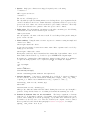
Contents
5 Placing two-terminal elements . . . . 14
5.1 Series and parallel circuits . . . . . 15
1 Introduction . . . . . . . . . . . . . . . . . . . . .
1
2 Using the macros . . . . . . . . . . . . . . . .
2.1 Quick start . . . . . . . . . . . . .
2.1.1 Processing with dpic and
PSTricks or Tikz PGF . . .
2.1.2 Processing with gpic . . . .
2.1.3 Simplifications . . . . . . .
2.2 Including the libraries . . . . . . .
2
2
3 Pic essentials . . . . . . . . . . . . . . . . . . . . .
3.1 Manuals . . . . . . . . . . . . . . .
3.2 The linear objects: line, arrow,
spline, arc . . . . . . . . . . . .
3.3 Positions . . . . . . . . . . . . . . .
3.4 The planar objects:
box,
circle, ellipse, and text . . . .
3.5 Compound objects . . . . . . . . .
3.6 Other language facilities . . . . . .
4 Two-terminal circuit elements
4.1 Circuit and element basics . .
4.2 The two-terminal elements . .
4.3 Branch-current arrows . . . .
4.4 Labels . . . . . . . . . . . . .
1
....
. . .
. . .
. . .
. . .
6 Composite circuit elements . . . . . . . 17
6.1 Semiconductors . . . . . . . . . . . 22
7 Corners . . . . . . . . . . . . . . . . . . . . . . . . . . 25
3
8 Looping . . . . . . . . . . . . . . . . . . . . . . . . . .
3
4 9 Logic gates . . . . . . . . . . . . . . . . . . . . . . .
5
10 Element and diagram scaling . . . . .
10.1 Circuit scaling . . . . . . . . . . .
6
10.2 Pic scaling . . . . . . . . . . . . . .
6
26
26
30
30
30
11 Writing macros . . . . . . . . . . . . . . . . . . 31
6
7 12 Interaction with LAT X . . . . . . . . . . . 34
E
7 13 PSTricks and other tricks . . . . . . . .
8
8 14 Web documents, pdf, and alternative output formats . . . . . . . . . . . . . .
9
15 Developer’s notes . . . . . . . . . . . . . . . .
9
10 16 Bugs . . . . . . . . . . . . . . . . . . . . . . . . . . . . .
13
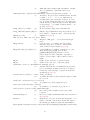
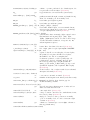
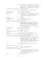
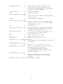
14 17 List of macros . . . . . . . . . . . . . . . . . . . .
37
37
38
39
42
Introduction
It appears that people who are unable to execute pretty pictures with pen and paper
find it gratifying to try with a computer [10].
This manual describes a method for drawing electric circuits and other diagrams in LATEX and
web documents. The diagrams are defined in the simple pic drawing language [9] augmented
with m4 macros [8], and are processed by m4 and a pic processor to convert them to PSTricks,
Tikz PGF, other LATEX-compatible code, or SVG. In its basic form, the method has the advantages
and disadvantages of TEX itself, since it is macro-based and non-WYSIWYG, with ordinary text
input. The book from which the above quotation is taken correctly points out that the payoff can
be in quality of diagrams at the price of the time spent in learning how to draw them.
A collection of basic components, most based on IEEE standards [6], and conventions for their
internal structure are described. Macros such as these are only a starting point, since it is often
convenient to customize elements or to package combinations of them for particular drawings.
1
2
Using the macros
This section describes the basic process of adding circuit diagrams to LATEX documents to produce
postscript or pdf files. On some operating systems, project management software with graphical
interfaces can be used to automate the process but the steps can be performed by a script, makefile,
or by hand for simple documents as described in Section 2.1.
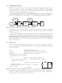
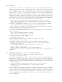
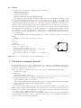
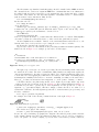
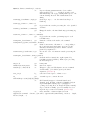
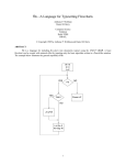
The diagram source file is preprocessed as illustrated in Figure 1. The predefined macros,
followed by the diagram source, are read by m4. The result is passed through a pic interpreter to
produce .tex output that can be inserted into a .tex document using the \input command.
.tex
files
.m4
macros
.m4
diagram
m4
LATEX
or
PDFlatex
pic
interpreter
.dvi
or
.pdf
Figure 1: Inclusion of figures and macros in the LATEX document.
The interpreter output contains PSTricks [16] commands, Tikz PGF [15] commands, basic LATEX
graphics, tpic specials, or other formats, depending on the chosen options, These variations are
described in Section 14.
There are two principal choices of pic interpreter. One is dpic, described later in this document.
A partial alternative is GNU gpic -t (sometimes simply named pic) [11] together with a printer driver
that understands tpic specials, typically dvips [13]. The dpic processor extends the pic language in
small but important ways; consequently, some of the macros and examples in this distribution work
fully only with dpic. Pic processors contain basic macro facilities, so some of the concepts applied
here do not require m4.
2.1
Quick start
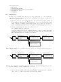
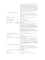
The contents of file quick.m4 and resulting diagram are shown in Figure 2 to illustrate the language,
to show several ways for placing circuit elements, and to provide sufficient information for producing
basic labeled circuits.
.PS
# Pic input begins with .PS
cct_init
# Read in macro definitions and set defaults
elen = 0.75
# Variables are allowed; default units are inches
Origin: Here
# Position names are capitalized
source(up_ elen); llabel(-,v_s,+)
resistor(right_ elen); rlabel(,R,)
dot
{
# Save the current position and direction
capacitor(down_ to (Here,Origin))
#(Here,Origin) = (Here.x,Origin.y)
rlabel(+,v,-); llabel(,C,)
dot
}
# Restore position and direction
R
+
line right_ elen*2/3
+
vs
v
inductor(down_ Here.y-Origin.y); rlabel(,L,); b_current(i)
−
line to Origin
−
.PE
# Pic input ends
i
C
L
Figure 2: The file quick.m4 and resulting diagram. There are several ways of drawing the same picture;
for example, nodes (such as Origin) can be defined and circuit branches drawn between them; or
absolute coordinates can be used (e.g., source(up_ from (0,0) to (0,0.75)) ). Element sizes
and styles can be varied as described in later sections.
2
To process the file, make sure that the libraries libcct.m4 and libgen.m4 are installed and
readable. Verify that m4 is installed and accepts the -I option; otherwise, see page 42. Now there
are at least two basic possibilities as follows, but be sure to read Section 2.1.3 for simplified use.
2.1.1
Processing with dpic and PSTricks or Tikz PGF
If you are using dpic with PSTricks, type the following commands or put them into a script:
m4 -I installdir pstricks.m4 quick.m4 > quick.pic
dpic -p quick.pic > quick.tex
where installdir is the full name (i.e., the path) of the directory containing libcct.m4. The
option -I installdir can be omitted if environment variable M4PATH points to installdir. Put
\usepackage{pstricks} in the main LATEX source file header and the following in the body:
\begin{figure}[hbt]
\centering
\input quick
\caption{Customized caption for the figure.}
\label{Symbolic_label}
\end{figure}
Then the commands latex file; dvips file produce file.ps that can be printed or viewed using
gsview, for example.
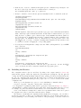
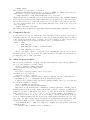
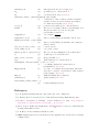
The effect of the m4 command above is shown in Figure 3. Configuration file pstricks.m4 causes
library libgen.m4 to be read, thereby defining the macro cct_init. The diagram source file is
then read and the circuit-element macros in libcct.m4 are defined during expansion of cct_init.
pstricks.m4
.pic
m4
libgen.m4
Configuration file
Diagram source quick.m4
···
define(‘cct_init’,...)
···
libcct.m4
···
define(‘resistor’,...)
···
.PS
cct_init
···
Figure 3: The command m4 -I installdir pstricks.m4 quick.m4 > quick.pic.
To produce Tikz PGF code, the commands are modified to read pgf.m4 and invoke the -g
option of dpic as follows:
m4 -I installdir pgf.m4 quick.m4 > quick.pic
dpic -g quick.pic > quick.tex
The LATEX header should contain \usepackage{tikz}, but the inclusion statements are the
same as for PSTricks input. Invoking PDFlatex on the source produces .pdf output directly.
In all cases the essential line is \input quick, which inserts the previously created file quick.tex.
2.1.2
Processing with gpic
If your printer driver understands tpic specials and you are using gpic (on some systems the gpic
command is pic), the commands are
m4 -I installdir gpic.m4 quick.m4 > quick.pic
gpic -t quick.pic > quick.tex
and the figure inclusion statements are as shown:
3
\begin{figure}[hbt]
\input quick
\centerline{\box\graph}
\caption{Customized caption for the figure.}
\label{Symbolic_label}
\end{figure}
2.1.3
Simplifications
m4 must read a configuration file followed by the macro definitions in one or more library files,
either before reading the diagram source file or at the beginning of it. There are several ways to
control the process, as follows:
1. The macros can be processed by LATEX-specific project software and by graphic applications
such as Cirkuit [7]. Alternatively when many files are to be processed, a facility such as Unix
“make,” which is also available in PC and Mac versions, can be employed to automate the
required commands. On systems without such facilities, a scripting language can be used.
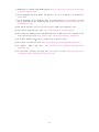
2. The m4 commands illustrated above can be shortened to
m4 -I installdir quick.m4 > quick.pic
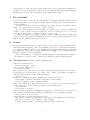
by inserting include(pstricks.m4) (assuming PSTricks processing) or include(libgen.m4)
(assuming the default processor is to be used) after the .PS line. The effect of the first include
statement is shown in Figure 4 and the second in Figure 5.
Diagram source
.pic
m4
pstricks.m4
.PS
include(pstricks.m4)
cct_init
···
Configuration file
libgen.m4
···
define(‘cct_init’,...)
···
libcct.m4
···
define(‘resistor’,...)
···
Figure 4: The command m4 -I installdir quick.m4 > quick.pic, with include(pstricks.m4) preceding cct_init.
Diagram source
.pic
m4
.PS
include(libgen.m4)
cct_init
···
libgen.m4
if..include(pstricks.m4)
···
define(‘cct_init’,...)
···
pstricks.m4
Configuration file
libcct.m4
···
define(‘resistor’,...)
···
Figure 5: The command m4 -I installdir quick.m4 > quick.pic, with include(libgen.m4) preceding
cct_init, causing the default configuration file to be read.
3. On some systems, setting the environment variable M4PATH to installdir allows the -I installdir
option of m4 to be omitted, but it will be kept in following examples.
4
4. In the absence of a need to examine the file quick.pic, the commands for producing the .tex
file can be reduced (provided the above inclusions have been made) to
m4 -I installdir quick.m4 | dpic -p > quick.tex
5. It may be desirable to invoke m4 and dpic automatically from the document file as shown:
\documentclass{article}
\usepackage{tikz}
\newcommand\mtotex[2]{\immediate\write18{m4 #2.m4 | dpic -#1 > #2.tex}}%
\begin{document}
\mtotex{g}{FileA} % Generate FileA.tex
\input{FileA.tex} \par
\mtotex{g}{FileB} % Generate FileB.tex
\input{FileB.tex}
\end{document}
The first argument of \mtotex is a p for pstricks or g for pgf. Sources FileA.m4 and FileB.m4
must contain any required include statements, and the main document should be processed
using the latex or pdflatex option -shell-escape. If the M4PATH environment variable is
not set then insert -I installdir after m4 in the command definition, where installdir is the
absolute path to the installation directory. This method processes the picture source each
time LATEX is run, so for large documents containing many diagrams, the \mtotex lines could
be commented out after debugging the corresponding graphic.
6. You can put several diagrams into a single source file. Make each diagram the body of a LATEX
macro, as shown:
\newcommand{\diaA}{%
.PS
drawing commands
.PE
\box\graph }% \box\graph not required for dpic
\newcommand{\diaB}{%
.PS
drawing commands
.PE
\box\graph }% \box\graph not required for dpic
Produce a .tex file using \mtotex or m4 and dpic or gpic, insert the .tex into the LATEX
source, and invoke the macros \diaA and \diaB at the appropriate places.
2.2
Including the libraries
The configuration files for dpic are as follows, depending on the output format (see Section 14):
pstricks.m4, pgf.m4, mfpic.m4, mpost.m4, postscript.m4, psfrag.m4, svg.m4, gpic.m4,
or xfig.m4. The file psfrag.m4 simply defines the macro psfrag_ and then reads postscript.m4.
For gpic, the configuration file is gpic.m4. The usual case for producing circuit diagrams is to read
pstricks.m4 or pgf.m4 first when dpic is the postprocessor or to set one of these as the default
configuration file.
At the top of each diagram source, put one or more initialization commands; that is,
cct_init, log_init, sfg_init, darrow_init, threeD_init
or, for diagrams not requiring specialized macros, gen_init. As shown in Figure 3 to Figure 5,
each initialization command reads in the appropriate macro library if it hasn’t already been read;
for example, cct_init tests whether libcct.m4 has been read and includes it if necessary.
A few of the distributed example files contain other experimental macros that can be pasted
into diagram source files; see Flow.m4 or Buttons.m4, for example.
The libraries contain hints and explanations that might help in debugging or if you wish to
modify any of the macros. Macros are generally named using the obvious circuit element names so
that programming becomes something of an extension of the pic language. Some macro names end
5
in an underscore to reduce the chance of name clashes. These can be invoked in the diagram source
but there is no long-term guarantee that their names and functionality will remain unchanged.
Finally, macros intended only for internal use begin with the characters m4.
3
Pic essentials
Pic source is a sequence of lines in a file. The first line of a diagram begins with .PS with optional
following arguments, and the last line is normally .PE. Lines outside of these pass through the pic
processor unchanged.
The visible objects can be divided conveniently into two classes, the linear objects line, arrow,
spline, arc, and the planar objects box, circle, ellipse.
The object move is linear but draws nothing. A compound object, or block, is planar and
consists of a pair of square brackets enclosing other objects, as described in Section 3.5. Objects
can be placed using absolute coordinates or relative to other objects.
Pic allows the definition of real-valued variables, which are alphameric names beginning with
lower-case letters, and computations using them. Objects or locations on the diagram can be given
symbolic names beginning with an upper-case letter.
3.1
Manuals
The classic pic manual [9] is still a good introduction to pic, but a more complete manual [12] can be
found in the GNU groff package, and both are available on the web [9, 12]. Reading either will give
you competence with pic in an hour or two. Explicit mention of *roff string and font constructs in
these manuals should be replaced by their equivalents in the LATEX context. A man-page language
summary is appended to the dpic manual [1].
A web search will yield good discussions of “little languages”; for pic in particular, see Chapter 9
of [2]. Chapter 1 of reference [4] also contains a brief discussion of this and other languages.
3.2
The linear objects: line, arrow, spline, arc
A line can be drawn as follows:
line from position to position
where position is defined below or
line direction distance
where direction is one of up, down, left, right. When used with the m4 macros described here,
it is preferable to add an underscore: up_, down_, left_, right_. The distance is a number or
expression and the units are inches, but the assignment
scale = 25.4
has the effect of changing the units to millimetres, as described in Section 10.
Lines can also be drawn to any distance in any direction. The example,
line up_ 3/sqrt(2) right_ 3/sqrt(2) dashed
draws a line 3 units long from the current location, at a 45◦ angle above horizontal. Lines (and
other objects) can be specified as dotted, dashed, or invisible, as above.
The construction
line from A to B chop x
truncates the line at each end by x (which may be negative) or, if x is omitted, by the current circle
radius, which is convenient when A and B are circular graph nodes, for example. Otherwise
line from A to B chop x chop y
truncates the line by x at the start and y at the end.
Any of the above means of specifying line (or arrow) direction and length will be called a linespec.
Lines can be concatenated. For example, to draw a triangle:
line up_ sqrt(3) right_ 1 then down_ sqrt(3) right_ 1 then left_ 2
6
3.3
Positions
A position can be defined by a coordinate pair, e.g. 3,2.5, more generally using parentheses by
(expression, expression), as a sum or difference as position + (expression, expression), or by the
construction (position, position), the latter taking the x-coordinate from the first position and
the y-coordinate from the second. A position can be given a symbolic name beginning with an
upper-case letter, e.g. Top: (0.5,4.5). Such a definition does not affect the calculated figure
boundaries. The current position Here is always defined and is equal to (0, 0) at the beginning of a
diagram or block. The coordinates of a position are accessible, e.g. Top.x and Top.y can be used in
expressions. The center, start, and end of linear objects (and the defined points of other objects as
described below) are predefined positions, as shown in the following example, which also illustrates
how to refer to a previously drawn element if it has not been given a name:
line from last line.start to 2nd last arrow.end then to 3rd line.center
Objects can be named (using a name commencing with an upper-case letter), for example:
Bus23: line up right
after which, positions associated with the object can be referenced using the name; for example:
arc cw from Bus23.start to Bus23.end with .center at Bus23.center
An arc is drawn by specifying its rotation, starting point, end point, and center, but sensible
defaults are assumed if any of these are omitted. Note that
arc cw from Bus23.start to Bus23.end
does not define the arc uniquely; there are two arcs that satisfy this specification. This distribution
includes the m4 macros
arcr( position, radius, start radians, end radians)
arcd( position, radius, start degrees, end degrees)
arca( chord linespec, ccw|cw, radius, modifiers)
to draw uniquely defined arcs. For example,
arcd((1,1),2,0,-90) -> cw
draws a clockwise arc with centre at (1, 1), radius 2, from (3, 1) to (1, −1), and
arca(from (1,1) to (2,2),,1,->)
draws an acute angled arc with arrowhead on the chord defined by the first argument.
The linear objects can be given arrowheads at the start, end, or both ends, for example:
line dashed <- right 0.5
arc <-> height 0.06 width 0.03 ccw from Here to Here+(0.5,0) \
with .center at Here+(0.25,0)
spline -> right 0.5 then down 0.2 left 0.3 then right 0.4
The arrowheads on the arc above have had their shape adjusted using the height and width
parameters.
3.4
The planar objects: box, circle, ellipse, and text
Planar objects are drawn by specifying the width, height, and position, thus:
A: box ht 0.6 wid 0.8 at (1,1)
after which, in this example, the position A.center is defined, and can be referenced simply as A.
In addition, the compass corners A.n, A.s, A.e, A.w, A.ne, A.se, A.sw, A.nw are automatically
defined, as are the dimensions A.height and A.width. Planar objects can also be placed by
specifying the location of a defined point; for example, two touching circles can be drawn as shown:
circle radius 0.2
circle diameter (last circle.width * 1.2) with .sw at last circle.ne
The planar objects can be filled with gray or colour. For example, the line
box dashed fill
produces a dashed box filled with a medium gray by default. The gray density is controlled using
the fill_(number) macro, where 0 ≤ number ≤ 1, with 0 corresponding to black and 1 to white.
Basic colours for lines and fills are provided by gpic and dpic, but more elaborate line and fill
styles can be incorporated, depending on the printing device, by inserting \special commands or
other lines beginning with a backslash in the drawing code. In fact, arbitrary lines can be inserted
into the output using
7
command "string"
where string is one or more lines to be inserted.
Arbitrary text strings, typically meant to be typeset by LATEX, are delimited by double-quote
characters and occur in two ways. The first way is illustrated by
"\large Resonances of $C_{20}H_{42}$" wid x ht y at position
which writes the typeset result, like a box, at position and tells pic its size. The default size assumed
by pic is given by parameters textwid and textht if it is not specified as above. The exact typeset
size of formatted text can be obtained as described in Section 12. The second occurrence associates
one or more strings with an object, e.g., the following writes two words, one above the other, at the
centre of an ellipse:
ellipse "\bf Stop" "\bf here"
The C-like pic function sprintf("format string",numerical arguments) is equivalent to a string.
3.5
Compound objects
A compound object is a group of statements enclosed in square brackets. Such an object is placed
by default as if it were a box, but it can also be placed by specifying the final position of a defined
point. A defined point is the center or compass corner of the bounding box of the compound object
or one of its internal objects. Consider the last line of the code fragment shown:
Ands: [ right_
And1: AND_gate
And2: AND_gate at And1 - (0,And1.ht*3/2)
...
] with .And2.In1 at position
The two gate macros evaluate to compound objects containing Out, In1, and other locations.
The final positions of all objects inside the square brackets are determined in the last line by
specifying the position of In1 of gate And2.
3.6
Other language facilities
All objects have default sizes, directions, and other characteristics, so part of the specification of
an object can sometimes be profitably omitted.
Another possibility for defining positions is
expression between position and position
which means
1st position + expression × (2nd position − 1st position)
and which can be abbreviated as
expression < position , position >
Care has to be used in processing the latter construction with m4, since the comma may have to
be put within quotes, ‘,’ to distinguish it from the m4 argument separator.
Positions can be calculated using expressions containing variables. The scope of a position is
the current block. Thus, for example,
theta = atan2(B.y-A.y,B.x-A.x)
line to Here+(3*cos(theta),3*sin(theta)).
Expressions are the usual algebraic combinations of primary quantities: constants, environmental parameters such as scale, variables, horizontal or vertical coordinates of terms such as
position.x or position.y, dimensions of pic objects, e.g. last circle.rad. The elementary algebraic operators are +, -, *, /, %, =, +=, -=, *=, /=, and %=, similar to the C language.
The logical operators ==, !=, <=, >=, >, and < apply to expressions and strings. A modest
selection of numerical functions is also provided: the single-argument functions sin, cos, log,
exp, sqrt, int, where log and exp are base-10, the two-argument functions atan2, max, min,
and the random-number generator rand(). Other functions are also provided using macros.
A pic manual should be consulted for details, more examples, and other facilities, such as the
branching facility
if expression then { anything } else { anything },
8
the looping facility
for variable = expression to expression by expression do { anything },
operating-system commands, pic macros, and external file inclusion.
4
Two-terminal circuit elements
There is a fundamental difference between the two-terminal elements, each of which is drawn on
an invisible straight-line segment, and other elements, which are compound objects mentioned in
Section 3.5. The two-terminal element macros follow a set of conventions described in this section,
and other elements will be described in Section 6.
4.1
Circuit and element basics
A list of the library macros and their arguments is in Section 17. The arguments have default
values, so that only those that differ from defaults need be specified.
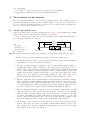
Figure 6, which shows a resistor, also serves as an example of pic commands. The first part of
the source file for this figure is on the left:
.PS
cct_init
linewid = 2.0
linethick_(2.0)
R1: resistor
elen_
dimen_
R1.start
R1.centre
last []
R1.end
Figure 6: Resistor named R1, showing the size parameters, enclosing block, and predefined positions.
The lines of Figure 6 and the remaining source lines of the file are explained below:
• The first line invokes the macro cct_init that loads the library libcct.m4 and initializes
local variables needed by some circuit-element macros.
• The sizes of circuit elements are multiples of the pic environmental variable linewid, so
redefining this variable changes element sizes. The element body is drawn in proportion to
dimen_, a macro that evaluates to linewid unless redefined, and the default element length
is elen_, which evaluates to dimen_*3/2 unless redefined. Setting linewid to 2.0 as in the
example means that the default element length becomes 3.0 in. For resistors, the default
length of the body is dimen_/2, and the width is dimen_/6. All of these values can be
customized. Element scaling and the use of SI units is discussed further in Section 10.
• The macro linethick_ sets the default thickness of subsequent lines (to 2.0 pt in the example).
Macro arguments are written within parentheses following the macro name, with no space
between the name and the opening parenthesis. Lines can be broken before macro arguments
because m4 and dpic ignore white space immediately preceding arguments. Otherwise, a long
line can be continued to the next by putting a backslash as the rightmost character.
• The two-terminal element macros expand to sequences of drawing commands that begin with
‘line invis linespec’, where linespec is the first argument of the macro if it is non-blank,
otherwise the line is drawn a distance elen_ in the current direction, which is to the right
by default. The invisible line is first drawn, then the element is drawn on top of it. The
element—rather, the initial invisible line—can be given a name, R1 in the example, so that
positions R1.start, R1.centre, and R1.end are automatically defined as shown.
• The element body is overlaid by a block, which can be used to place labels around the
element. The block corresponds to an invisible rectangle with horizontal top and bottom
lines, regardless of the direction in which the element is drawn. A dotted box has been drawn
in the diagram to show the block boundaries.
9
• The last sub-element, identical to the first in two-terminal elements, is an invisible line that
can be referenced later to place labels or other elements. If you create your own macros, you
might choose simplicity over generality, and include only visible lines.
To produce Figure 6, the following embellishments were added after the previously shown source:
thinlines_
box dotted wid last [].wid ht last [].ht at last []
move to 0.85 between last [].sw and last [].se
spline <- down arrowht*2 right arrowht/2 then right 0.15; "\tt last []" ljust
arrow <- down 0.3 from R1.start chop 0.05; "\tt R1.start" below
arrow <- down 0.3 from R1.end chop 0.05; "\tt R1.end" below
arrow <- down last [].c.y-last arrow.end.y from R1.c; "\tt R1.centre" below
dimension_(from R1.start to R1.end,0.45,\tt elen\_,0.4)
dimension_(right_ dimen_ from R1.c-(dimen_/2,0),0.3,\tt dimen\_,0.5)
.PE
• The line thickness is set to the default thin value of 0.4 pt, and the box displaying the element
body block is drawn. Notice how the width and height can be specified, and the box centre
positioned at the centre of the block.
• The next paragraph draws two objects, a spline with an arrowhead, and a string left justified
at the end of the spline. Other string-positioning modifiers than ljust are rjust, above,
and below.
• The last paragraph invokes a macro for dimensioning diagrams.
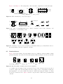
4.2
The two-terminal elements
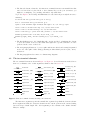
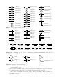
The two-terminal elements are shown in Figure 7 to Figure 12. Several elements are included more
than once to illustrate some of their arguments, which are listed in Section 17.
resistor
resistor(,,Q)
resistor(,,ES)
resistor(,4,QR)
resistor(,,E)
≡ ebox
resistor(,,H)
resistor(,,V)
ebox(,,,0.5)
ebox(,0.5,0.3)
inductor
inductor(,W)
inductor(,L)
inductor(,,,M)
inductor(,W,6,P)
capacitor
capacitor(,C)
capacitor(,C+)
capacitor(,P)
capacitor(,E)
capacitor(,K)
capacitor(,M)
capacitor(,N)
xtal
memristor
heater
tline
gap
gap(,,A)
arrowline
G
ttmotor(,G)
Figure 7: Basic two-terminal elements, showing some variations.
The first macro argument specifies the invisible line segment along which the element is drawn.
If the argument is blank, the element is drawn from the current position in the current drawing
direction along a default length. The other arguments produce variants of the default elements.
Thus, for example,
10
source
source(,,0.4)
source(,I)
source(,P)
source(,i)
− +
source(,V)
source(,v)
source(,AC)
source(,U)
consource
source(,R)
consource(,I)
source(,S)
consource(,i)
source(,T)
source(,X)
µA
source(,N)
source(,
"\micro{}A")
−+
consource(,V)
source(,L)
consource(,v)
source(,F)
source(,B)
battery
source(,G)
nullator
battery(,3,R)
source(,Q)
norator
Figure 8: Sources and source-like elements.
diode(,CR)
diode(,K)
diode(,L)
diode(,F)
diode(,Sh)
diode(,D)
diode
diode(,S)
diode(,V)
diode(,v)
diode(,w)
diode(,B)
diode(,G)
diode(,Z,RE)
diode(,T)
diode(,P)
diode(,LE)
diode(,LER)
Figure 9: The macro diode(linespec,B|CR|D|K|L|LE[R]|P[R]|S|T|V|v|w|Z,[R][E]).
fuse
fuse(,D)
fuse(,B)
fuse(,C)
fuse(,S)
fuse(,HB)
(,HC,0.5,0.3)
cbreaker
cbreaker(,R)
. . .(,,D)
. . .(,,T)
. . .(,,TS)
Figure 10:
Variations of the macros fuse(linespec, A|dA|B|C|D|E|S|HB|HC, wid, ht) and
cbreaker(linespec,L|R,D|T|TS).
amp
delay
amp(,0.3)
delay(,0.2)
integrator
integrator(,0.3)
Figure 11: Amplifier, delay, and integrator.
resistor(up_ 1.25,7)
draws a resistor 1.25 units long up from the current position, with 7 vertices per side. The macro
up_ evaluates to up but also resets the current directional parameters to point up.
Most of the two-terminal elements are oriented; that is, they have a defined polarity. Several element macros include an argument that reverses polarity, but there is also a more general
mechanism, as follows.
11
lswitch
(,,O)
(,,C)
(,,D)
(,,DO)
(,,DC)
(,,K)
(,,KD)
(,,KOD)
(,,KCD)
bswitch
(,,C)
(,,WBuD)
(,,WBF)
W B
dB
dswitch=
switch(,,,D)
(,,WdBK)
(,,WdBKL)
K
(,,WBT)
(,,WdBKC)
(,,WdBKF)
(,,WBL)
(,,WBM)
(,,WBCO)
(,,WBMP)
(,,WBRHH)
(,,WBCY)
(,,WBCZ)
(,,WBCE)
(,,WBRH)
(,,WBRdH)
(,,WBMMR)
(,,WBMM)
(,,WBMR)
(,,WBEL)
(,,WBLE)
(,,WdBKEL)
Figure 12:
The switch(linespec,L|R,chars,L|B|D) macro is a wrapper for the macros
lswitch(linespec,[L|R],[O|C][D][K]), bswitch(linespec,[L|R],[O|C]), and the many-optioned
dswitch(linespec,R,W[ud]B[K] chars) shown. The switch is drawn in the current drawing direction. A second-argument R produces a mirror image with respect to the drawing direction.
The first argument of the macro
reversed(‘macro name’,macro arguments)
is the name of a two-terminal element in quotes, followed by the element arguments. The element
is drawn with reversed direction. Thus,
diode(right_ 0.4); reversed(‘diode’,right_ 0.4)
draws two diodes to the right, but the second one points left.
Similarly, the macro
resized(factor,‘macro name’,macro arguments)
can be used to resize the body of an element by temporarily multiplying the dimen_ macro by
factor. More general resizing should be done by redefining dimen_ as described in Section 10.1.
These two macros can be nested; the following scales the above example by 1.8, for example
resized(1.8,‘diode’,right_ 0.4); resized(1.8,‘reversed’,‘diode’,right_ 0.4)
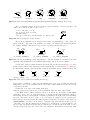
Figure 13 contains arrows for indicating radiation effects. The arrow stems are named A1, A2,
and each pair is drawn in a [] block, with the names Head and Tail defined to aid placement near
another device. The second argument specifies absolute angle in degrees (default 135 degrees).
A2
Head
A1
Tail
em_arrows(N)
em_arrows(ND,45) . . .(I)
. . .(ID)
. . .(E)
. . .(ED)
Figure 13: Radiation arrows: em_arrows(type, angle, length)
Figure 14 shows some two-terminal elements with arrows or lines overlaid to indicate variability
using the macro
variable(‘element’,type,angle,length),
where type is one of A, P, L, N, with C or S optionally appended to indicate continuous or stepwise
variation. Alternatively, this macro can be invoked similarly to the label macros in Section 4.4 by
12
specifying an empty first argument; thus, the following line draws the resistor in Figure 14:
resistor(down_ dimen_); variable(,uN)
C
S
A
P
L
N
Figure 14: Illustrating variable(‘element’,[A|P|L|[u]N][C|S],angle,length).
For example,
variable(‘capacitor(down_ dimen_)’) draws the leftmost capacitor shown above, and
variable(‘resistor(down_ dimen_)’,uN) draws the resistor. The default angle is 45◦ , regardless
of the direction of the element. The array on the right shows the effect of the second argument.
4.3
Branch-current arrows
Arrowheads and labels can be added to conductors using basic pic statements. For example, the
following line adds a labeled arrowhead at a distance alpha along a horizontal line that has just
been drawn. Many variations of this are possible:
arrow right arrowht from last line.start+(alpha,0) "$i_1$" above
Macros have been defined to simplify labelling two-terminal elements, as shown in Figure 15.
The macro
b_current(label, above_|below_, In|O[ut], Start|E[nd], frac)
draws an arrow from the start of the last-drawn two-terminal element frac of the way toward the
body.
i
i
b_current(i)
i
. . .(i,below_)
i
b_current(i,,,E)
i
i
. . .(i,below_,,E)
. . .(i,,O,E,0.2)
i
larrow(i)
i
. . .(i,below_,O)
. . .(i,,O)
i
. . .(i,below_,O,E)
i
i
rarrow(i)
larrow(i,<-)
i
rarrow(i,<-)
Figure 15: Illustrating b_current, larrow, and rarrow. The drawing direction is to the right.
If the fourth argument is End, the arrow is drawn from the end toward the body. If the third
element is Out, the arrow is drawn outward from the body. The first argument is the desired label,
of which the default position is the macro above_, which evaluates to above if the current direction
is right or to ljust, below, rjust if the current direction is respectively down, left, up. The label
is assumed to be in math mode unless it begins with sprintf or a double quote, in which case it
is copied literally. A non-blank second argument specifies the relative position of the label with
respect to the arrow, for example below_, which places the label below with respect to the current
direction. Absolute positions, for example below or ljust, also can be specified.
For those who prefer a separate arrow to indicate the reference direction for current, the macros
larrow(label, ->|<-,dist) and rarrow(label, ->|<-,dist) are provided. The label is placed outside the arrow as shown in Figure 15. The first argument is assumed to be in math mode unless it
begins with sprintf or a double quote, in which case the argument is copied literally. The third
argument specifies the separation from the element.
13
4.4
Labels
Special macros for labeling two-terminal elements are included:
llabel( arg1,arg2,arg3 )
clabel( arg1,arg2,arg3 )
rlabel( arg1,arg2,arg3 )
dlabel( long,lat,arg1,arg2,arg3,[X][A|B][L|R])
The first macro places the three arguments, which are treated as math-mode strings, on the
left side of the element block with respect to the current direction: up, down, left, right. The
second places the arguments along the centre, and the third along the right side. A simple circuit
example with labels is shown in Figure 16. The macro dlabel performs these functions for an
obliquely drawn element, placing the three macro arguments at vec_(-long,lat), vec_(0,lat),
and vec_(long,lat) respectively relative to the centre of the element. In the fourth argument,
an X aligns the labels with respect to the line joining the two terminals rather than the element
body, and A, B, L, R use absolute above, below, left, or right alignment respectively for the
labels. Labels beginning with sprintf or a double quote are copied literally rather than assumed
to be in math mode.
Arbitrary LATEX including \includegraphics, for example, can also be placed on a diagram
using
"LATEX text" wid width ht height at position
.PS
# ‘Loop.m4’
cct_init
define(‘dimen_’,0.75)
loopwid = 1; loopht = 0.75
source(up_ loopht); llabel(-,v_s,+)
resistor(right_ loopwid); llabel(,R,); b_current(i)
inductor(down_ loopht,W); rlabel(,L,)
capacitor(left_ loopwid,C); llabel(+,v_C,-); rlabel(,C,)
.PE
i
R
+
vs
L
−
C
− +
vC
Figure 16: A loop containing labeled elements, with its source code.
5
Placing two-terminal elements
The length and position of a two-terminal element are defined by a straight-line segment and,
possibly, a direction, so four numbers are required to place the element as in the following example:
resistor(from (1,1) to (2,1)).
However, pic has a very useful concept of the current point (explicitly named Here); thus,
resistor(to (2,1))
is equivalent to
resistor(from Here to (2,1)).
Any defined position can be used; for example, if C1 and L2 are names of previously defined
two-terminal elements, then, for example, the following places the resistor:
resistor(from L2.end to C1.start)
A line segment starting at the current position can also be defined using a direction and length.
To draw a resistor up d units from the current position, for example:
resistor(up_ d)
Pic stores the current drawing direction, the latter unfortunately limited to up, down, left,
right, which is assumed when necessary. The circuit macros need to know the current direction,
so whenever up, down, left, right are used they should be written respectively as the macros
up_, down_, left_, right_ as in the above example.
To allow drawing circuit objects in other than the standard four directions, a transformation
matrix is applied at the macro level to generate the required pic code. Potentially, the matrix can
be used for other transformations. The macro
14
setdir_(direction, default direction)
is preferred when setting drawing direction. The direction arguments are of the form
R[ight] | L[eft] | U[p] | D[own] | degrees,
but the macros Point_(degrees), point_(radians), and rpoint_(relative linespec) are employed
in many macros to re-define the entries of the matrix (named m4a_, m4b_, m4c_, and m4d_) for
the required rotation. The macro eleminit_ in the two-terminal elements invokes rpoint_ with a
specified or default linespec to establish element length and direction.
As shown in Figure 17, ‘Point_(-30); resistor’ draws a resistor along a line with slope of -30
degrees, and ‘rpoint_(to Z)’ sets the current direction cosines to point from the current location
to location Z. Macro vec_(x,y) evaluates to the position (x,y) rotated as defined by the argument
of the previous setdir_, Point_, point_ or rpoint_ command. The principal device used to
define relative locations in the circuit macros is rvec_(x,y), which evaluates to position Here +
vec_(x,y). Thus, line to rvec_(x,0) draws a line of length x in the current direction.
Figure 17 illustrates that some hand placement of labels using dlabel may be useful when
elements are drawn obliquely. The figure also illustrates that any commas within m4 arguments
must be treated specially because the arguments are separated by commas. Argument commas are
protected either by parentheses as in inductor(from Cr to Cr+vec_(elen_,0)), or by multiple
single quotes as in ‘‘,’’, as necessary. Commas also may be avoided by writing 0.5 between L
and T instead of 0.5<L,T>.
.PS
# ‘Oblique.m4’
cct_init
Ct:dot; Point_(-60); capacitor(,C); dlabel(0.12,0.12,,,C_3)
Cr:dot; left_; capacitor(,C); dlabel(0.12,0.12,C_2,,)
Cl:dot; down_; capacitor(from Ct to Cl,C); dlabel(0.12,-0.12,,,C_1)
R1
T:dot(at Ct+(0,elen_))
inductor(from T to Ct); dlabel(0.12,-0.1,,,L_1)
Point_(-30); inductor(from Cr to Cr+vec_(elen_,0))
dlabel(0,-0.07,,L_3,)
R:dot
L:dot( at Cl-(R.x-Cr.x,Cr.y-R.y) )
u
y
L1
R3
+
C1
C3
−
C2
L2
inductor(from L to Cl); dlabel(0,-0.12,,L_2,)
right_; resistor(from L to R); rlabel(,R_2,)
resistor(from T to R); dlabel(0,0.15,,R_3,) ; b_current(y,ljust)
line from L to 0.2<L,T>
source(to 0.5 between L and T); dlabel(sourcerad_+0.07,0.1,-,,+)
dlabel(0,sourcerad_+0.07,,u,)
resistor(to 0.8 between L and T); dlabel(0,0.15,,R_1,)
line to T
L3
R2
.PE
Figure 17: Illustrating elements drawn at oblique angles.
5.1
Series and parallel circuits
To draw elements in series, each element can be placed by specifying its line segment as described
previously, but the pic language makes some geometries particularly simple. Thus,
setdir_(Right)
resistor; llabel(,R); capacitor; llabel(,C); inductor; llabel(,L)
draws three elements in series as shown in the top line of Figure 18. However, the default length
elen_ appears too long for some diagrams. It can be redefined temporarily (to dimen_, say), by
enclosing the above line in the pair
pushdef(‘elen_’,dimen_), . . . popdef(‘elen_’)
15
C
R
C
R
C
R
L
L
L
Figure 18: Three ways of drawing basic elements in series.
with the result shown in the middle row of the figure.
Alternatively, the length of each element can be tuned individually; for example, the capacitor
in the above example can be shortened as shown, producing the bottom line of Figure 18:
resistor; llabel(,R)
capacitor(right_ dimen_/4); llabel(,C)
inductor; llabel(,L)
If a macro that takes care of common cases automatically is to be preferred, you can use the
macro series_(elementspec, elementspec, . . .). This macro draws elements of length dimen_ from
the current position in the current drawing direction, enclosed in a [ ] block. The internal names
Start, End, and C (for centre) are defined, along with any element labels. An elementspec is of
the form [Label:] element; [attributes], where an attribute is zero or more of llabel(. . .),
rlabel(. . .), or b_current(. . .).
Drawing elements in parallel requires a little more effort but, for example, three elements can
be drawn in parallel using the code snippet shown, producing the left circuit in Figure 19:
define(‘elen_’,dimen_)
L: inductor(right_ 2*elen_,W); llabel(+,L,-)
R1: resistor(right elen_ from L.start+(0,-dimen_)); llabel(,R1)
R2: resistor; llabel(,R2)
C: capacitor(right 2*elen_ from R1.start+(0,-dimen_)); llabel(,C)
line from L.start to C.start
line from L.end to C.end
Start
R1
+ L −
+
R2
V
R1
−
R2
C
L
End
Start
setdir_(Down)
parallel_(
series_(‘R1:resistor; rlabel(,R_1)’,
parallel_(
series_(‘resistor; rlabel(,R_2)’,
‘inductor(,W); rlabel(,L)’),
‘capacitor(,C); rlabel(,C)’ ),
line down dimen_/2),
‘Sep=linewid*3/2; V:source; rlabel(+,V,-)’)
C
End
parallel_( ‘L:inductor(,W); llabel(+,L,-)’,
series_(‘R1:resistor; llabel(,R1)’, ‘R2:resistor; llabel(,R2)’),
‘C:capacitor; llabel(,C)’ )
Figure 19: Illustrating the macros parallel_ and series_, with Start and End points marked.
A macro that produces the same effect automatically is
parallel_(‘elementspec’, ‘elementspec’, . . .)
The arguments should be quoted to delay expansion, unless an argument is a nested parallel_
macro, in which case it is not quoted. The elements are drawn in a [ ] block with defined points
Start, End, and C. An elementspec is of the form
[Sep=val;][Label:] element; [attributes]
16
where an attribute is of the form
[llabel(. . .);] | [rlabel(. . .)] | [b_current(. . .);]
Putting Sep=val; in the first branch sets the default separation of all branches to val; in a
later element, Sep=val; applies only to that branch. An element may have normal arguments
but should not change the drawing direction. An element may also be series_(args) or nested
parallel_(args) without quotes, as illustrated in Figure 19.
6
Composite circuit elements
Many basic elements are not two-terminal. These elements are usually enclosed in a [ ] pic block,
and contain named interior locations and components. The block must be placed by using its
compass corners, thus: element with corner at position or, when the block contains a predefined
location, thus: element with location at position. A few macros are positioned with the first
argument; the ground macro, for example: ground(at position). In some cases, an invisible line
can be specified by the first argument to determine length and direction (but not position) of the
block.
Nearly all elements drawn within blocks can be customized by adding an extra argument, which
is executed as the last item within the block.
The macro potentiometer(linespec,cycles,fractional pos,length, . . .), shown in Figure 20,
first draws a resistor along the specified line, then adds arrows for taps at fractional positions along
the body, with default or specified length. A negative length draws the arrow from the right of the
current drawing direction.
Start
Start
T1
End
Start
T1
T1
T2
End
End
...(down_ dimen_,,0.5,-5mm__)
potentiometer(down_ dimen_)
...(down_ dimen_,,0.25,-5mm__,0.75,5mm__)
Figure 20: Default and multiple-tap potentiometer.
The macro addtaps([arrowhd | type=arrowhd;name=Name], fraction, length, fraction, length,
. . .), shown in Figure 21, will add taps to the immediately preceding two-terminal element. However,
R1.start
Tap1
R3.Start
R3.Tap1
L1.Tap1
Tap2
right_; t = 0.2in__
R1.end R1: resistor(,,E)
addtaps(<-,0.2,-t,0.8,t)
R3.End
Tx1
R2: ebox(,elen_*0.6)
addtaps(type=-;name=Tx,
Tx3
0.2,-t,0.5,-t,0.8,-t)
R3: tapped(‘ebox(,elen_*0.6,)’,->,0.2,-t,0.5,-t,0.8,-t) \
with .Start at R1.start+(0.25in__,-0.6in__)
R3.Tap3
L1.Tap4
L1: tapped(‘inductor(right_ 9*dimen_/8,,9)’,
-,0,-t,3/9,-t/2,6/9,-t/2,1,-t)
Figure 21: Macros for adding taps to two-terminal elements.
the default names Tap1, Tap2 . . . may not be unique in the current scope. An alternative name
for the taps can be specified or, if preferable, the tapped element can be drawn in a [ ] block using
the macro tapped(‘two-terminal element’, [arrowhd | type=arrowhd;name=Name], fraction,
length, fraction, length, . . .). Internal names .Start, .End, and .C are defined automatically,
corresponding to the drawn element. These and the tap names can be used to place the block.
17
These two macros require the two-terminal element to be drawn either up, down, to the left, or to
the right; they are not designed for obliquely drawn elements.
A few composite symbols derived from two-terminal elements are shown in Figure 22.
T1
Start
Start T1 T2 End
KelvinR
T1
T2
KelvinR(,R)
End
T1
Start
T2
FTcap
End
Start
End
Start
T
FTcap(D)
T
FTcap(C)
T2
FTcap(B)
End
Figure 22: Composite elements KelvinR(cycles,[R],cycle wid) and FTcap(chars) .
The ground symbol is shown in Figure 23. The first argument specifies position; for example,
the two lines shown have identical effect:
move to (1.5,2); ground
ground(at (1.5,2))
The second argument truncates the stem, and the third defines the symbol type. The fourth
argument specifies the angle at which the symbol is drawn, with D (down) the default. This macro
is one of several in which a temporary drawing direction is set using the setdir_( U|D|L|R|degrees,
default R|L|U|D|degrees ) macro and reset at the end using resetdir_.
ground
ground(,T)
(,,F)
(,,E)
(,,S)
(,,S,90)
(,,Q)
(,,L)
(,,P)
Figure 23: The ground( at position, T, N|F|S|L|P|E, U|D|L|R|degrees ) macro.
The arguments of the macro antenna( at position, T, A|L|T|S|D|P|F, U|D|L|R|degrees )
shown in Figure 24 are similar to those of ground.
(,,L)
antenna
(,T)
T
T
T1
T2
(,,S)
(,T,L)
T1
T2
(,,T)
T
(,,D)
T1
T2
T1
T2
(,,P)
(,,F)
T
T
Figure 24: Antenna symbols, with macro arguments shown above and terminal names below.
Figure 25 illustrates the macro opamp(linespec, - label, + label, size, chars). The element
is enclosed in a block containing the predefined internal locations shown. These locations can
be referenced in later commands, for example as ‘last [].Out.’ The first argument defines the
direction and length of the opamp, but the position is determined either by the enclosing block of
the opamp, or by a construction such as ‘opamp with .In1 at Here’, which places the internal
position In1 at the specified location. There are optional second and third arguments for which the
defaults are \scriptsize$-$ and \scriptsize$+$ respectively, and the fourth argument changes
the size of the opamp. The fifth argument is a string of characters. P adds a power connection, R
exchanges the second and third entries, and T truncates the opamp point.
Typeset text associated with circuit elements is not rotated by default, as illustrated by the
second and third opamps in Figure 25. The opamp labels can be rotated if necessary by using
postprocessor commands (for example PSTricks \rput) as second and third arguments.
The code in Figure 26 places an opamp with three connections.
Figure 27 shows variants of the transformer macro, which has predefined internal locations P1,
P2, S1, S2, TP, and TS. The first argument specifies the direction and distance from P1 to P2,
with position determined by the enclosing block as for opamps. The second argument places the
secondary side of the transformer to the left or right of the drawing direction. The optional third
18
N
In1
V1
E1
E
−
W
Out
+
In2
−
+
−
E2
S
opamp
−
V2
+
+
Point_(15); opamp(,,,,PR)
opamp(,,,,T)
Point_(90); opamp
Figure 25: Operational amplifiers. The P option adds power connections. The second and third arguments
can be used to place and rotate arbitrary text at In1 and In2.
line right 0.2 then up 0.1
A: opamp(up_,,,0.4,R) with .In1 at Here
line right 0.2 from A.Out
line down 0.1 from A.In2 then right 0.2
+
−
Figure 26: A code fragment invoking the opamp(linespec,-,+,size,[R][P]) macro.
and fifth arguments specify the number of primary and secondary arcs respectively. If the fourth
argument string contains an A, the iron core is omitted; if a P, the core is dashed (powder); and if
it contains a W, wide windings are drawn. A D1 puts phase dots at the P1, S1 end, D2 at the P2, S2
ends, and D12 or D21 puts dots at opposite ends.
P1
P1
S1
P1
S1
P1
S1
P1
S1
S1
TP
TS
TP
TS
TP
TS
TP
TS
TS
TP
P2
S2
transformer
P2
S2
...(down_ 0.6„2,P,8)
S2
P2
...(„8,WD12,4)
P2
S2
...(„9,AL)
S2
P2
...(,R,8,AW)
Figure 27: The transformer(linespec,L|R,np,[A|P][W|L][D1|D2|D12|D21],ns) macro (drawing direction down), showing predefined terminal and centre-tap points.
Figure 28 shows some audio devices, defined in [] blocks, with predefined internal locations as
shown. The first argument specifies the device orientation.
Face
Box Circle
Circle
Box
In1
In1
In1
In1
In2
In2
In2
In2
Box
In4 In5
In3
In3
In3
In3
In1
microphone
buzzer(,,C)
bell
buzzer
Box
In2
N
In1
In3
L
R
In2
C
In6 In7
In3
speaker . . .(,,H)
earphone
earphone(,,C)
Figure 28: Audio components: speaker(U|D|L|R|degrees,size,type), bell, microphone, buzzer,
earphone, with their internally named positions and components.
Thus,
S: speaker(U) with .In2 at Here
places an upward-facing speaker with input In2 at the current location.
The nport(box specs [; other commands], nw, nn, ne, ns, space ratio, pin lgth, style) macro
is shown in Figure 29. The macro begins with the line define(‘nport’,‘[Box: box ‘$1’, so the
first argument is a box specification such as size, fill, or text. The second to fifth arguments specify
the number of ports (pin pairs) to be drawn respectively on the west, north, east, and south sides
of the box. The end of each pin is named according to the side, port number, and a or b pin, as
shown. The sixth argument specifies the ratio of port width to inter-port space, the seventh is the
19
N1a
N1b N2a
N2b
E1a
E1a W1a
W1a
n-port
W1b
..
.
W1
E1
E1b W1b
E3b
nport
···
S1a
S4b
nport(wid 2.0 ht 1 fill_(0.9) "n-port",1,2,3,4)
S1
nterm
Figure 29: The nport macro draws a sequence of pairs of named pins on each side of a box. The pin
names are shown. The default is a twoport. The nterm macro draws single pins instead of pin
pairs.
pin length, and setting the eighth argument to N omits the pin dots. The macro ends with ‘$9’]’),
so that a ninth argument can be used to add further customizations within the enclosing block.
The nterm(box specs, nw, nn, ne, ns, pin lgth, style) macro illustrated in Figure 29 is similar to
the nport macro but has one fewer argument, draws single pins instead of pin pairs, and defaults
to a 3-terminal box.
Many custom labels or added elements may be required, particularly for 2-ports. These elements
can be added using the first argument and the ninth of the nport macro. For example, the following
code adds a pair of labels to the box immediately after drawing it but within the enclosing block:
nport(; ‘"0"’ at Box.w ljust; ‘"∞"’ at Box.e rjust)
If this trick were to be used extensively, then the following custom wrapper would save typing,
add the labels, and pass all arguments to nport:
define(‘nullor’,‘nport(‘$1’
{‘"${}0$"’ at Box.w ljust
‘"$\infty$"’ at Box.e rjust},shift($@))’)
The above example and the related gyrator macro are illustrated in Figure 30.
0
∞
nullor
gyrator
gyrator(invis,,0,N)
gyrator(invis wid boxht,,0,NV)
Figure 30: The nullor example and the gyrator macro are customizations of the nport macro.
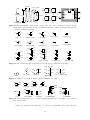
A basic winding macro for magnetic-circuit sketches and similar figures is shown in Figure 31.
For simplicity, the complete spline is first drawn and then blanked in appropriate places using the
background (core) color (lightgray for example, default white).
Figure 32 shows the macro contact(chars), which contains predefined locations P, C, O for the
armature and normally closed and normally open terminals. An I in the first argument draws open
circles for contacts. The macro relay(poles, chars, R) defines coil terminals V1, V2 and contact
terminals Pi , Ci , Oi .
The double-throw switches shown in Figure 33 are drawn in the current drawing direction like
the two-terminal elements, but are composite elements that must be placed accordingly.
The jack and plug macros and their defined points are illustrated in Figure 34. The first
argument of both macros establishes the drawing direction. The second argument is a string of
characters defining drawn components. An R in the string specifies a right orientation with respect
to the drawing direction. The two principal terminals of the jack are included by putting L S or
both into the string with associated make (M) or break (B) points. Thus, LMB within the third
argument draws the L contact with associated make and break points. Repeated L[M|B] or S[M|B]
substrings add auxiliary contacts with specified make or break points.
20
pitch
core color
T1
T1
T2
T2
φ
Left pins Left pins +
cw
ccw
v1
core wid
T2
T2 −
winding
diam
T1
winding(R)
T1
i1
i2
g
N1
N2
T1
Right pins Right pins
cw
ccw
T2
Figure 31: The winding(L|R, diam, pitch, turns, core wid, core color) macro draws a coil with
axis along the current drawing direction. Terminals T1 and T2 are defined. Setting the first argument
to R draws a right-hand winding.
C
C
O
P
P
P
O
C
O
contact(C,)
contact(O,)
contact(,R)
contact
contact(P)
C
O
P
P
contact(I)
C1
P1
O
C
contact(RI)
C2
P2
O2
C1
P1
O1
V1
O1
V2
V1
relay
C
P
V2
relay(2)
O
contact(PI)
V1
P1
P2
contact(CI)
contact(OI)
V2
O1
C1
O2
C2
relay(2,RIP)
relay(2,O)
relay(2,CT)
Figure 32: The contact(O|C,R) and relay(poles,O|C,R) macros (default direction right).
R
T
L
up_; NPDT
L T R
NPDT
L1
R1
R2
L2
R2
L1
R1
NPDT(2)
L3
R3
L2
NPDT(3,R)
R2
L2
R1
L1
left_; NPDT(2,R)
Figure 33: Multipole double-throw switches drawn by NPDT(npoles, [R]).
TB
B
A
TA
plug
A
B
plug(,R)
LM
L
F
G
jack
LB
B
C
A
plug(,3)
B
C
A
plug(L,3R)
L
L
S
S
jack(,LMBS)
..(L,RLS)
LM2
L2 LM1
L1
L
LB
S
..(L,RLBLMLMS)
SM1
S1
SB S
LB L
..(,RSBSMLB)
Figure 34: The jack(U|D|L|R|degrees, chars) and plug(U|D|L|R|degrees,[2|3][R]) components and
their defined points.
A macro for drawing headers is in Figure 35, and some experimental connectors are shown in
21
+
v2
−
Figure 36 and Figure 37. The tstrip macro allows key=value; arguments for width and height.
P15
P8
P1
P2
Header
P1
P1
PinP1
PinP2
P2
P1
P5
P6
P16
P2
down_; Header(2,8)
Header(2,3,8mm__,10mm__)
left_; Header(2,4,,,fill_(0.9))
Figure 35: Macro Header(1|2, rows, wid, ht, type).
T4
.. R4
. ..
.
T1
R1
L4
..
.
L1
tstrip(U)
···
T1
ccoax(,F)
T5
tstrip(R,5,
DO;wid=1.0;ht=0.25)
C
S
ccoax
tconn(,O)
tconn(,<)
(,«)
(,>)
(,»)
Figure 36: Macros tstrip(R|L|U|D|degrees, chars), ccoax(at location, M|F, diameter), and
tconn(linespec, >|»|<|«|O[F], wid).
N
H
N
G
G
pconnex(,A)
H
(,AF)
(,G)
(,AC)
(,GF)
(,ACF)
(L,GF)
(,P)
(U,D) (U,DF) (U,J) (U,JF)
(,GC)
Figure 37: A small set of power connectors drawn by pconnex(R|L|U|D|degrees, chars). Each connector
has an internal H, N, and where applicable, a G shape.
6.1
Semiconductors
Figure 38 shows the variants of bipolar transistor macro bi_tr(linespec,L|R,P,E) which contains
predefined internal locations E, B, C. The first argument defines the distance and direction from E
C
C
C
B
C
B
E
B
E
E
bi_tr(,R)
bi_tr(up_ dimen_)
bi_tr(,,P)
C
B
C
G
G
E
bi_tr(,,,E)
E
E
igbt(,,LD)
igbt
Figure 38: Bipolar transistor variants (current direction upward).
to C, with location determined by the enclosing block as for other elements, and the base placed
to the left or right of the current drawing direction according to the second argument. Setting the
third argument to ‘P’ creates a PNP device instead of NPN, and setting the fourth to ‘E’ draws
an envelope around the device. Figure 39 shows a composite macro with several optional internal
elements.
22
C
C
C
B
B
C
B
B1
E B1
(R,DZB1)
E
Darlington
E
(,EB1)
C
B
B
B1
B1
E
(,EB1DZR1)
E
(,EB1DE1E2)
Figure 39: Macro Darlington(L|R,[E][P][B1][E1|R1][E2|R2][D][Z]), drawing direction up_.
The code fragment example in Figure 40 places a bipolar transistor, connects a ground to the
emitter, and connects a resistor to the collector.
S: dot; line left_ 0.1; up_
Q1: bi_tr(,R) with .B at Here
ground(at Q1.E)
line up 0.1 from Q1.C; resistor(right_ S.x-Here.x); dot
Figure 40: The bi_tr(linespec,L|R,P,E) macro.
The bi_tr and igbt macros are wrappers for the macro bi_trans(linespec, L|R, chars, E),
which draws the components of the transistor according to the characters in its third argument.
For example, multiple emitters and collectors can be specified as shown in Figure 41.
SB
uE
B
BU
S
Em2
B
B
Cm2
C
E C
bi_trans(,,BCuEBUS)
C
E2 E1 E0
bi_trans(,,BCdE2BU)
E
C0 C1 C2
bi_trans(,,BC2dEBU)
Figure 41: The bi_trans(linespec,L|R,chars,E) macro. The sub-elements are specified by the third
argument. The substring En creates multiple emitters E0 to En. Collectors are similar.
A UJT macro with predefined internal locations B1, B2, and E is shown in Figure 42, and a
thyristor macro with predefined internal locations G and T1, T2, or A, K is in Figure 43. Except for
the G terminal, a thyristor (the IEC variant excluded) is much like an two-terminal element. The
B2
B2
B2
B2
E
E
E
E
B1
ujt(up_ dimen_,,,E)
B1
ujt(,,P,)
B1
ujt(,R,,)
B1
ujt(,R,P,)
Figure 42: UJT devices, with current drawing direction up_.
wrapper macro scr(linespec, chars, label) and similar macros scs, sus, and sbs place thyristors
using linespec as for a two-terminal element, but require a third argument for the label for the
compound block; thus,
scr(from A to B,,Q3); line right from Q3.G
draws the element from position A to position B with label Q3, and draws a line from G.
Some FETs with predefined internal locations S, D, and G are also included, with similar
arguments to those of bi_tr, as shown in Figure 44. In all cases the first argument is a linespec,
and entering R as the second argument orients the G terminal to the right of the current drawing
direction. The macros in the top three rows of the figure are wrappers for the general macro
mosfet(linespec,R,characters,E). The third argument of this macro is a subset of the characters
{BDEFGLMQRSTXZ}, each letter corresponding to a diagram component as shown in the bottom row
of the figure. Preceding the characters B, G, and S by u or d adds an up or down arrowhead to the
pin, preceding T by d negates the pin, and preceding M by u or d puts the pin at the drain or source
end respectively of the gate. The obsolete letter L is equivalent to dM and has been kept temporarily
23
A
T1
T1
T1
A
A
T1
A
A
A
G
G
G
K
K
T2
K
K
K
K
T2
...(,IEC)
...(,F)
...(,UARE)
thyristor
...(,BR)
...(,B)
...(,BE)...(,A)
...(,BRE)
...(,AV)
G
G G
A
T2 G
A
G
A Ga
Ga
A
G
G
A
G T2
A
Ga A
Ga A
A
T1
G
G
G
G
G
G
K
K
K
K
K
K
K
K
K
T2
...(,N)
...(,SCR)
...(SCRRE)
...(SCSE)
...(SBSE)
...(,UAH)
...(,UANRE)
...(SCRE)
...(SCS)
...(SUSE)
G
Q.G
scr(,,Q)
Q3.G
sus(,RE,Q3)
Q2.G
scs(,,Q2)
sbs(,E,Q4)
Q4.G
Q2.Ga
Figure 43: The top two rows illustrate use of the thyristor(linespec, chars) macro, drawing direction
down_, and the bottom row shows wrapper macros (drawing direction right_) that place the
thyristor like a two-terminal element.
for compatibility. This system allows considerable freedom in choosing or customizing components,
as illustrated in Figure 44.
G
G
S
D
S
D S
D
G
j_fet(,,P,) e_fet(,R,,) d_fet(,,,)
j_fet(right_ dimen_,,,E)
G0
G1
G1
c_fet(,,,)
e_fet(,,,S)
d_fet(,,,S)
G0
...(,,dBSDFQuM1)
d_fet(,,P)
d_fet(,,P,S)
c_fet(,,P)
e_fet(,,P)
e_fet(,,P,S)
mosfet(,,dBSDFQM1,E)
D
G
uH
dG
dM
dT
F
uB
G
E
Z
S
D
S
D
Q
B
mosfet(,,dGSDF,)
S
. . .(,,ZSDFdT,)
. . .(,,dMEDSQuB,)
. . .(,,uMEDSuB)
. . .(,,uHSDF,)
IRF4905
Figure 44: JFET, insulated-gate enhancement and depletion MOSFETs, and simplified versions. These
macros are wrappers that invoke the mosfet macro as shown in the middle and bottom rows.
The two lower-right examples show custom devices, the first defined by omitting the substrate
connection, and the second defined using a wrapper macro.
The number of possible semiconductor symbols is very large, so these macros must be regarded
as prototypes. Often an element is a minor modification of existing elements. For example, the
thyristor(linespec, chars) macro illustrated in Figure 43 is derived from the diode and bipolar
transistor macros. Another example is the tgate macro shown in Figure 45, which also shows a
pass transistor.
24
Gb
Gb
tgate
A
B
G
G
tgate(,L)
A
A
A
G
A
tgate(,B)
Gb
ptrans
B
ptrans(,L)
G G
B
B
B
Gb
Figure 45: The tgate(linespec, [B][R|L]) element, derived from a customized diode and ebox, and the
ptrans(linespec, [R|L]) macro. These are not two-terminal elements, so the linespec argument
defines the direction and length of the line from A to B but not the element position.
Some other non-two-terminal macros are dot, which has an optional argument ‘at location’,
the line-thickness macros, the fill_ macro, and crossover, which is a useful if archaic method to
show non-touching conductor crossovers, as in Figure 46.
Vcc
RL
R1
RL
R1
Q1
Q2
R2
R2
−Vcc
Figure 46: Bipolar transistor circuit, illustrating crossover and colored elements.
This figure also illustrates how elements and labels can be colored using the macro
rgbdraw(r, g, b, drawing commands)
where the r, g, b values are in the range 0 to 1 (integers from 0 to 255 for SVG) to specify the rgb
color. This macro is a wrapper for the following, which may be more convenient if many elements
are to be given the same color:
setrgb(r, g, b)
drawing commands
resetrgb
A macro is also provided for colored fills:
rgbfill(r, g, b, drawing commands)
These macros depend heavily on the postprocessor and are intended only for PSTricks, Tikz PGF,
MetaPost, SVG, and the Postscript or PDF output of dpic.
7
Corners
If two straight lines meet at an angle then, depending on the postprocessor, the corner may not be
mitred or rounded unless the two lines belong to a multisegment line, as illustrated in Figure 47. This
line up 0.2
line right 0.2
line up 0.2 \
then right 0.2
line up 0.15 left 0.15
corner
line up 0.1 right 0.1
line up 0.2
line right 0.2 \
chop -hlth chop 0
line up 0.2
round
line right 0.2
B
A
corner(,at A)
L
M
Mitre_(L,M,5 bp__)
Figure 47: Producing mitred angles and corners.
25
C
A
mitre_(A,B,C)
is normally not an issue for circuit diagrams unless the figure is magnified or thick lines are drawn.
Rounded corners can be obtained by setting post-processor parameters, but the figure shows the effect of macros round and corner. The macros mitre_(Position1,Position2,Position3,length,attributes)
and Mitre_(Line1,Line2,length,attributes) may assist as shown. Otherwise, a rght-angle line can
be extended by half the line thickness (macro hlth) as shown on the upper row of the figure, or a
two-segment line can be overlaid at the corner to produce the same effect.
8
Looping
Sequential actions can be performed using either the dpic command
for variable=expression to expression [by expression] do { actions }
or at the m4 processing stage. The libgen library defines the macro
for_(start, end, increment, ‘actions’)
for this and other purposes. Nested loops are allowed and the innermost loop index variable is m4x.
The first three arguments must be integers and the end value must be reached exactly; for example,
for_(1,3,2,‘print In‘’m4x’) prints locations In1 and In3, but for_(1,4,2,‘print In‘’m4x’)
does not terminate since the index takes on values 1, 3, 5, . . ..
Repetitive actions can also be performed with the libgen macro
Loopover_(‘variable’, actions, value1, value2, . . .)
which evaluates actions for each instance of variable set to value1, value2, . . ..
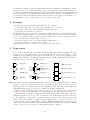
9
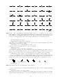
Logic gates
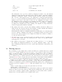
Figure 48 shows the basic logic gates included in library liblog.m4. The first argument of the gate
macros can be an integer N from 0 to 16, specifying the number of input locations In1, . . . InN,
as illustrated for the NOR gate in the figure. By default, N = 2 except for macros NOT_gate and
BUFFER_gate, which have one input In1 unless they are given a first argument, which is treated as
the line specification of a two-terminal element.
AND_gate
OR_gate
NAND_gate
In1
In2
In3
BUFFER_gate
XOR_gate
Out
NOR_gate(3)
N_Out
NOT_gate
In1
In2
In3
&
NAND_gate(,B)
≥1
NOR_gate(3,NB)
=1
BOX_gate(PN,N,,,=1)
=
NXOR_gate(NPN)
BOX_gate(PP,N,,,=)
Figure 48: Basic logic gates. The input and output locations of a three-input NOR gate are shown.
Inputs are negated by including an N in the second argument letter sequence. A B in the second
argument produces a box shape as shown in the rightmost column, where the second example has
AND functionality and the bottom two are examples of exclusive OR functions.
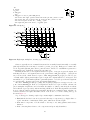
Input locations retain their positions relative to the gate body regardless of gate orientation, as
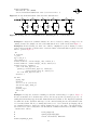
in Figure 49. Beyond a default number (6) of inputs, the gates are given wings as in Figure 50.
Negated inputs or outputs are marked by circles drawn using the NOT_circle macro. The name
marks the point at the outer edge of the circle and the circle itself has the same name prefixed by
N_. For example, the output circle of a nand gate is named N_Out and the outermost point of the
circle is named Out. Instead of a number, the first argument can be a sequence of letters P or N
to define normal or negated inputs; thus for example, NXOR_gate(NPN) defines a 3-input nxor gate
with not-circle inputs In1 and In3 and normal input In2 as shown in the figure. The macro IOdefs
can also be used to create a sequence of custom named inputs or outputs.
26
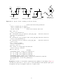
.PS
# ‘FF.m4’
S
log_init
S: NOR_gate
left_
R: NOR_gate at S+(0,-L_unit*(AND_ht+1))
line from S.Out right L_unit*3 then down S.Out.y-R.In2.y then to R.In2
line from R.Out left L_unit*3 then up S.In2.y-R.Out.y then to S.In2
line left 4*L_unit from S.In1 ; "$S$sp_" rjust
line right 4*L_unit from R.In1 ; "sp_$R$" ljust
.PE
Figure 49: SR flip-flop.
I0
I1
I2
I3
I4
I5
I6
R
I7
S2
S1
S0
Ē
Ȳ
Y
Figure 50: Eight-input multiplexer, showing a gate with wings.
Gates are typically not two-terminal elements and are normally drawn horizontally or vertically
(although arbitrary directions may be set with e.g. Point_(degrees)). Each gate is contained in a
block of typical height 6*L_unit where L_unit is a macro intended to establish line separation for
an imaginary grid on which the elements are superimposed.
Including an N in the second argument character sequence of any gate negates the inputs, and
including B in the second argument invokes the general macro BOX_gate([P|N]...,[P|N],horiz
size,vert size,label), which draws box gates. Thus, BOX_gate(PNP,N„8,\geq 1) creates a gate
of default width, eight L_units height, negated output, three inputs with the second negated, and
internal label “≥ 1”. If the fifth argument begins with sprintf or a double quote then the argument
is copied literally; otherwise it is treated as scriptsize mathematics.
The macro BUFFER_gate(linespec,[N|B],wid,ht,[N|P]*,[N|P]*) is a wrapper for the composite element BUFFER_gen. If the second argument is B, then a box gate is drawn; otherwise the
gate is triangular. Arguments 5 and 6 determine the number of defined points along the northeast
and southeast edges respectively, with an N adding a NOT circle. If the first argument is non-blank
however, then the buffer is drawn along an invisible line like a two-terminal element, which is convenient sometimes but requires internal locations of the block to be referenced using last [], as
shown in Figure 51.
A good strategy for drawing complex logic circuits might be summarized as follows:
• Establish the absolute locations of gates and other major components (e.g. chips) relative to
a grid of mesh size commensurate with L_unit, which is an absolute length.
• Draw minor components or blocks relative to the major ones, using parameterized relative
distances.
• Draw connecting lines relative to the components and previously drawn lines.
27
In1
NE
Out
N_NE1
N_NE2
In1
In1
In2
Out
C
SE
bd = dimen_*3/4
BUFFER_gate(,,bd,bd)
Out
C
N_SE1
BUFFER_gen(ITNOC,bd,bd,PN,,N,
LH_symbol at C)
BUFFER_gate(,N,bd,bd,NN)
BUFFER_gate(right_ elen_,,bd,bd)
BUFFER_gate(right_ elen_,N,bd,bd,,N,LH_symbol at C)
line down dimen_/3 from last [].N_SE1.s then left dimen_*2/3
Figure 51: The BUFFER_gate and BUFFER_gen macros. The bottom two examples show how the gate
can be drawn as a two-terminal macro but internal block locations must be referenced using last
[].
• Write macros for repeated objects.
• Tune the diagram by making absolute locations relative, and by tuning the parameters. Some
useful macros for this are the following, which are in units of L_unit:
AND_ht, AND_wd: the height and width of basic AND and OR gates
BUF_ht, BUF_wd: the height and width of basic buffers
N_diam: the diameter of NOT circles
Figure 52 shows a multiplexer block with variations, and Figure 53 shows the very similar
demultiplexer.
In0
0
In1
1
In2
2
In3
3
Sel0
Sel
0
M1
Out
Out
In0
In0
01
2
10
OE
Sel
NOE
Mux(4,M1)
left_; Mux(4,,LNOE)
In0
In7
00
1
3
Sel1
Sel0
11
In3
OE
OE
Mux(4,,OEBN2)
0
1
2
3
4
5
6
7
Sel2
down_; Mux(8,,L3,,28*L_unit)
Figure 52: The Mux(input count, label, [L][B|H][N[n]|S[n]][[N]OE],wid,ht) macro.
0
1
In
DM1
2
Sel
Out0
Out0 0
OE
1
Sel1
Out0
00
Sel0
OE
In In
01
2
In
Sel0
0
1
2
3
4
5
6
7
Sel2
OE
NOE
Out3
Out3
3
Out0
Out7
11
Sel
down_; Demux(8,,L3,,28*L_unit)
Demux(4,DM1)
(4,,NOEBN2)
left_; Demux(4,,LOE)
3
10
Figure 53: The Demux(input count, label, [L][B|H][N[n]|S[n]][[N]OE],wid,ht) macro.
28
Figure 54 shows the macro FlipFlop(D|T|RS|JK, label, boxspec), which is a wrapper for the
more general macro FlipFlopX(boxspec, label, leftpins, toppins, rightpins, bottompins). Each of
CLR
Q
D
Q1
CK
Q
T
J
Q
R
Q2
Q
Q
CK
CK
S
Q
Q
Q
K
PR
FlipFlop(D,Q1)
FlipFlop(RS)
FlipFlop(T,Q2,ht h1 wid w1 fill_(0.9))
FlipFlop(JK)
CLR
D
Q
J
Q
T
Q
CK
CK
CK
Q
FlipFlopX(,,
:D;E:CK,,:Q;:lg_bartxt(Q))
K
FlipFlopX(,,
:T;E:CK,,:Q;)
FlipFlopX(,,
:J;E:CK;:K,N:CLR,:Q;)
Figure 54: The FlipFlop and FlipFlopX macros, with variations.
arguments 3 to 6 is null or a string of pinspecs separated by semicolons (;). Pinspecs are either
empty (null) or of the form [pinopts]:[label[:Picname]]. The first colon draws the pin. Pins are
placed top to bottom or left to right along the box edges with null pinspecs counted for placement.
Pins are named by side and number by default; eg W1, W2, ..., N1, N2, ..., E1, ..., S1,
... ; however, if :Picname is present in a pinspec then Picname replaces the default name. A
pinspec label is text placed at the pin base. Semicolons are not allowed in labels; use eg \char59{}
instead, and to put a bar over a label, use lg_bartxt(label). The pinopts are [L|M|I|O][N][E]
as for the lg_pin macro.
Customized gates can be defined simply. For example, the following code defines the custom
flipflops in Figure 55.
PR4
PR3
PR2
PR1
PR0
PRESET
ENABLE
SERIAL
INPUT
PR
PR
Q
S
CK
R
R
PR
Q
S
CK
Q
CLR
PR
Q
S
CK
R
Q
CLR
CK
Q
CLR
PR
Q
S
R
Q
S
OUTPUT
CK
Q
R
CLR
CLR
CLEAR
CLOCK
Figure 55: A 5-bit shift register.
define(‘customFF’,‘FlipFlopX(wid 10*L_unit ht FF_ht*L_unit,,
:S;NE:CK;:R, N:PR, :Q;;ifelse(‘$1’,1,:lg_bartxt(Q)), N:CLR) ’)
This definition makes use of macros L_unit and FF_ht that predefine dimensions. There are three
pins on the right side; the centre pin is null and the bottom is null if the first macro argument is 1.
29
For hybrid applications, the dac and adc macros are illustrated in Figure 56. The figure shows
the default and predefined internal locations, the number of which can be specified as macro arguments.
N1
N1
N2
N1
N1
N2
NW
NE
NW
NE
Out3
Out1
In1
Out1 In1
In1
Out1 In1
DAC
Out2
ADC
Out2
C
C
In2
In2
Out1
Out3
SW
SE
SW
SE
S1
S1 S2 S3
S1
S1 S2 S3
dac
adc
Q: dac(,,2,2,3,3); "DAC" "2" at Q.C
adc(,,2,2,3,3)
Figure 56: The dac(width,height,nIn,nN,nOut,nS) and adc(width,height,nIn,nN,nOut,nS) macros.
In addition to the logic gates described here, some experimental IC chip diagrams are included
with the distributed example files.
10
Element and diagram scaling
There are several issues related to scale changes. You may wish to use millimetres, for example,
instead of the default inches. You may wish to change the size of a complete diagram while keeping
the relative proportions of objects within it. You may wish to change the sizes or proportions
of individual elements within a diagram. You must take into account that line widths are scaled
separately from drawn objects, and that the size of typeset text is independent of the pic language.
The scaling of circuit elements will be described first, then the pic scaling facilities.
10.1
Circuit scaling
The circuit elements all have default dimensions that are multiples of the pic environmental parameter linewid, so changing this parameter changes default element dimensions. The scope of a pic
variable is the current block; therefore, a sequence such as
resistor
T: [linewid = linewid*1.5; up_; Q: bi_tr] with .Q.B at Here
ground(at T.Q.E)
resistor(up_ dimen_ from T.Q.C)
connects two resistors and a ground to an enlarged transistor. Alternatively, you may redefine the
default length elen_ or the body-size parameter dimen_. For example, adding the line
define(‘dimen_’,(dimen_*1.2))
after the cct_init line of quick.m4 produces slightly larger body sizes for all circuit elements. For
logic elements, the equivalent to the dimen_ macro is L_unit, which has default value (linewid/10).
The macros capacitor, inductor, and resistor have arguments that allow the body sizes
to be adjusted individually. The macro resized mentioned previously can also be used.
10.2
Pic scaling
There are at least three kinds of graphical elements to be considered:
1. When generating final output after reading the .PE line, pic processors divide distances and
sizes by the value of the environmental parameter scale, which is 1 by default. Therefore, the
effect of assigning a value to scale at the beginning of the diagram is to change the drawing
unit (initially 1 inch) throughout the figure. For example, the file quick.m4 can be modified
to use millimetres as follows:
30
.PS
scale = 25.4
cct_init
# Pic input begins with .PS
# mm
# Set defaults
elen = 19
...
# Variables are allowed
The default sizes of pic objects are redefined by assigning new values to the environmental
parameters arcrad, arrowht, arrowwid, boxht, boxrad, boxwid, circlerad, dashwid,
ellipseht, ellipsewid, lineht, linewid, moveht, movewid, textht, and textwid.
The . . .ht and . . .wid parameters refer to the default sizes of vertical and horizontal lines,
moves, etc., except for arrowht and arrowwid, which are arrowhead dimensions. The boxrad
parameter can be used to put rounded corners on boxes. Assigning a new value to scale
also multiplies all of these parameters except arrowht, arrowwid, textht, and textwid by
the new value of scale (gpic multiplies them all). Therefore, objects drawn to default sizes
are unaffected by changing scale at the beginning of the diagram. To change default sizes,
redefine the appropriate parameters explicitly.
2. The .PS line can be used to scale the entire drawing, regardless of its interior. Thus, for example, the line .PS 100/25.4 scales the entire drawing to a width of 100 mm. Line thickness,
text size, and dpic arrowheads are unaffected by this scaling.
If the final picture width exceeds maxpswid, which has a default value of 8.5, then the picture
is scaled to this size. Similarly, if the height exceeds maxpsht (default 11), then the picture
is scaled to fit. These parameters can be assigned new values as necessary, for example, to
accommodate landscape figures.
3. The finished size of typeset text is independent of pic variables, but can be determined as in
Section 12. Then, "text" wid x ht y tells pic the size of text, once the printed width x
and height y have been found.
4. Line widths are independent of diagram and text scaling, and have to be set explicitly.
For example, the assignment linethick = 1.2 sets the default line width to 1.2 pt. The
macro linethick_(points) is also provided, together with default macros thicklines_ and
thinlines_.
11
Writing macros
The m4 language is quite simple and is described in numerous documents such as the original
reference [8] or in later manuals [14]. If a new circuit or other element is required, then it may
suffice to modify and rename one of the library definitions or simply add an option to it. Hints for
drawing general two-terminal elements are given in libcct.m4. However, if an element or block
is to be drawn in only one orientation then most of the elaborations used for general two-terminal
elements in Section 4 can be dropped. If you develop a library of custom macros in the installation
directory then the statement include(mylibrary.m4) can bring its definitions into play.
It may not be necessary to define your own macro if all that is needed is a small addition to
an existing element that is defined in an enclosing [ ] block. After the element arguments are
expanded, one argument beyond the normal list is automatically expanded before exiting the block,
as mentioned near the beginning of Section 6. This extra argument can be used to embellish the
element.
A macro is defined using quoted name and replacement text as follows:
define(‘name’,‘replacement text’)
After this line is read by the m4 processor, then whenever name is encountered as a separate
string, it is replaced by its replacement text, which may have multiple lines. The quotation characters are used to defer macro expansion. Macro arguments are referenced inside a macro by number;
thus $1 refers to the first argument. A few examples will be given.
31
define(‘thermalsw’,
‘dswitch(‘$1’,‘$2’,WDdBT)
circle rad distance(M4T,last line.c) at last line.c ’)
Figure 57: A custom thermal switch defined from the dswitch macro.
L
L
L
L
r
r
r
r
r
C
R
C
R
C
R
C
R
L
C
r
R
Figure 58: A lumped model of a transmission line, illustrating the use of custom macros.
Example 1: Custom two-terminal elements can often be defined by writing a wrapper for an
existing element. For example, an enclosed thermal switch can be defined as shown in Figure 57.
Example 2: In the following, two macros are defined to simplify the repeated drawing of a series
resistor and series inductor, and the macro tsection defines a subcircuit that is replicated several
times to generate Figure 58.
.PS
# ‘Tline.m4’
cct_init
hgt = elen_*1.5
ewd = dimen_*0.9
define(‘sresistor’,‘resistor(right_ ewd); llabel(,r)’)
define(‘sinductor’,‘inductor(right_ ewd,W); llabel(,L)’)
define(‘tsection’,‘sinductor
{ dot; line down_ hgt*0.25; dot
parallel_(‘resistor(down_ hgt*0.5); rlabel(,R)’,
‘capacitor(down_ hgt*0.5); rlabel(,C)’)
dot; line down_ hgt*0.25; dot }
sresistor ’)
SW: Here
gap(up_ hgt)
sresistor
for i=1 to 4 do { tsection }
line dotted right_ dimen_/2
tsection
gap(down_ hgt)
line to SW
.PE
Example 3: Composite elements containing several basic elements may be required. Figure 59
shows a circuit that can be drawn in any reference direction prespecified by Point_(degrees), containing labels that always appear in their natural horizontal orientation. Two flags in the argument
determine the circuit orientation with respect to the current drawing direction and whether a mirrored circuit is drawn. The key to writing such a macro is to observe that the pic language allows
two-terminal elements to change the current drawing direction, so the value of rp_ang should be
saved and restored as necessary after each internal two-terminal element has been drawn. A draft
of such a macro follows:
#
#
#
define(‘hybrid_PI_BJT’,
‘Point_(degrees)
hybrid_PI_BJT([L][M])
L=left orientation; M=mirror’
32
Base
ro
Collector
+
vπ rπ
gm vπ
−
ro
ro
gm vπ
+
rπ vπ
−
gm vπ
ro
Emitter
hybrid_PI_BJT
hybrid_PI_BJT(M)
rπ
−
vπ
+
hybrid_PI_BJT(LM)
+ rπ
vπ
−
gm vπ
Point_(45)
hybrid_PI_BJT
Figure 59: A composite element containing several basic elements
‘[
# Size (and direction) parameters:
hunit = ifinstr(‘$1’,M,-)dimen_
vunit = ifinstr(‘$1’,L,-)dimen_*3/2
hp_ang = rp_ang
# Save the reference direction
Base: dot(,,1)
line to rvec_(hunit/2,0)
Rpi: resistor(to rvec_(0,-vunit)); point_(hp_ang)
# Restore direction
line to rvec_(hunit*5/4,0)
Dot1: dot
Gm: consource(to rvec_(0,vunit),I,R); point_(hp_ang) # Restore direction
line to rvec_(hunit*3/4,0)
Ro: resistor(to rvec_(0,-vunit)); point_(hp_ang)
# Restore direction
line to Dot1
Dotro: dot(at Ro.start)
line to rvec_(hunit/2,0)
Collector: dot(,,1)
Dot2: dot(at 0.5 between Rpi.end and Dot1)
line to rvec_(0,-vunit/2)
Emitter: dot(,,1)
# Labels
‘"$\mathrm{r_\pi}$"’ at Rpi.c+vec_(hunit/4,0)
‘"$ + $"’ at Rpi.c+vec_(-hunit/6, vunit/4)
‘"$ - $"’ at Rpi.c+vec_(-hunit/6,-vunit/4)
‘"$\mathrm{v_\pi}$"’ at Rpi.c+vec_(-hunit/4,0)
‘"$\mathrm{g_m}$$\mathrm{v_\pi}$"’ at Gm.c+vec_(-hunit*3/8,-vunit/4)
‘"$\mathrm{r_o}$"’ at Ro.c+vec_(hunit/4,0)
‘$2’ ] ’)
Example 4: A number of elements have arguments meant explicitly for customization. Figure 60
customizes the source macro to show a cycle of a horizontal sinusoid with adjustable phase given
by argument 2 in degrees, as might be wanted for a 3-phase circuit:
33
define(‘phsource’,‘source($1,
#‘Set angle to 0, draw sinusoid, restore angle’
phsource(,120)
m4smp_ang = rp_ang; rp_ang = 0
sinusoid(m4h/2,twopi_/(m4h),
ifelse(‘$2’,,,‘($2)/360*twopi_+’)pi_/2,-m4h/2,m4h/2) with .Origin at Here
rp_ang = m4smp_ang,
$3,$4,$5)’)
Figure 60: A source element customized using its second argument.
Example 5: Repeated subcircuits might have different orientations but the potential orientations
often include only the element and its mirror image, so the power of the vec_() and rvec_() macros
is not required. Suppose that an optoisolator is to be drawn with left-right or right-left orientation
as shown in Figure 61.
A
C
C
K
E
E
A
B
K
Figure 61: Showing opto and opto(BR), with defined labels.
The macro interface could be something like the following:
opto( [L|R][A|B] ),
where an R in the argument string signifies a right-left (mirrored) orientation and the element is of
either A or B type; that is, there are two related elements that might be drawn in either orientation,
for a total of four possibilities. Those who find such an interface to be too cryptic might prefer to
invoke the macro as
opto(orientation=Rightleft;type=B),
which includes semantic sugar surrounding the R and B characters for readability; this usage is made
possible by testing the argument string using the ifinstr() macro rather than requiring an exact
match. A draft of the macro follows, and the file Optoiso.m4 in the examples directory adds a
third type option.
#
‘opto([R|L][A|B])’
define(‘opto’,‘[{u = dimen_/2
Q: bi_trans(up u*2,ifinstr(‘$1’,R,R),ifinstr(‘$1’,B,B)CBUdE)
E: Q.E; C: Q.C; A:ifinstr(‘$1’,R,Q.e+(u*3/2,u),Q.w+(-u*3/2,u)); K: A-(0,u*2)
ifinstr(‘$1’,B,line from Q.B to (Q.B,E); B: Here)
D: diode(from A to K)
arrow from D.c+(0,u/6) to Q.ifinstr(‘$1’,R,e,w)+(0,u/6) chop u/3 chop u/4
arrow from last arrow.start-(0,u/3) to last arrow.end-(0,u/3)
Enc: box rad u wid abs(C.x-A.x)+u*2 ht u*2 with .c at 0.5 between C and K
‘$2’ }]’)
Two instances of this subcircuit are drawn and placed by the following code, with the result shown
in Figure 61.
Q1: opto
Q2: opto(type=B;orientation=Rightleft) with .w at Q1.e+(dimen_,0)
12
Interaction with LATEX
The sizes of typeset labels and other TEX boxes are generally unknown prior to processing the
diagram by LATEX. Although they are not needed for many circuit diagrams, these sizes may be
34
required explicitly for calculations or implicitly for determining the diagram bounding box. The
following example shows how text sizes can affect the overall size of a diagram:
.PS
B: box
"Left text" at B.w rjust
"Right text: $x^2$" at B.e ljust
.PE
The pic interpreter cannot know the size of the text to the left and right of the box, and the
diagram is generated using default text values. One solution to this problem is to measure the text
sizes by hand and include them literally, thus:
"Left text" wid 38.47pt__ ht 7pt__ at B.w rjust
but this is tedious.
Often, a better solution is to process the diagram twice. The diagram source is processed as
usual by m4 and a pic processor, and the main document source is LATEXed to input the diagram
and format the text, and also to write the text dimensions into a supplementary file. Then the
diagram source is processed again, reading the required dimensions from the supplementary file and
producing a diagram ready for final LATEXing. This hackery is summarized below, with an example
in Figure 62.
.PS
gen_init
sinclude(CMman.dim)
s_init(stringdims)
B: box
s_box(Left text) at B.w rjust
s_box(Right text: $xˆ%g$,2) at B.e ljust
.PE
Left text
Right text: x2
Figure 62: The macro s_box sets string dimensions automatically when processed twice. If two or more
arguments are given to s_box, they are passed through sprintf. The dots show the figure bounding
box.
• Put \usepackage{boxdims} into the document source.
• Insert the following at the beginning of the diagram source, where jobname is the name of
the main LATEX file:
sinclude(jobname.dim)
s_init(unique name)
• Use the macro s_box(text) to produce typeset text of known size as shown in Figure 62;
alternatively, invoke the macros \boxdims and boxdim described later.
The macro s_box(text) evaluates initially to
"\boxdims{name}{text}" wid boxdim(name,w) ht boxdim(name,v)
On the second pass, this is equivalent to
"text" wid x ht y
where x and y are the typeset dimensions of the LATEX input text. If s_box is given two or more
arguments as in Figure 62 then they are processed by sprintf.
The argument of s_init, which should be unique within jobname.dim, is used to generate a
unique \boxdims first argument for each invocation of s_box in the current file. If s_init has been
omitted, the symbols “!!” are inserted into the text as a warning. Be sure to quote any commas in
the arguments. Since the first argument of s_box is LATEX source, make a rule of quoting it to avoid
comma and name-clash problems. For convenience, the macros s_ht, s_wd, and s_dp evaluate to
the dimensions of the most recent s_box string or to the dimensions of their argument names, if
present.
35
The file boxdims.sty distributed with this package should be installed where LATEX can find it.
The essential idea is to define a two-argument LATEX macro \boxdims that writes out definitions for
the width, height and depth of its typeset second argument into file jobname.dim, where jobname
is the name of the main source file. The first argument of \boxdims is used to construct unique
symbolic names for these dimensions. Thus, the line
box "\boxdims{Q}{\Huge Hi there!}"
has the same effect as
box "\Huge Hi there!"
except that the line
define(‘Q_w’,77.6077pt__)define(‘Q_h’,17.27779pt__)define(‘Q_d’,0.0pt__)dnl
is written into file jobname.dim (and the numerical values depend on the current font). These
definitions are required by the boxdim macro described below.
The LATEX macro
\boxdimfile{dimension file}
is used to specify an alternative to jobname.dim as the dimension file to be written. This simplifies
cases where jobname is not known in advance or where an absolute path name is required.
Another simplification is available. Instead of the sinclude(dimension file) line above, the
dimension file can be read by m4 before reprocessing the source for the second time:
m4 library files dimension file diagram source file ...
Objects can be tailored to their attached text by invoking \boxdims and boxdim explicitly. The
small source file in Figure 63, for example, produces the box in the figure.
.PS
# ‘eboxdims.m4’
sinclude(CMman.dim) # The main input file is CMman.tex
box fill_(0.9) wid boxdim(Q,w) + 5pt__ ht boxdim(Q,v) + 5pt__ \
"\boxdims{Q}{\large$\displaystyle\int_0^T e^{tA}\,dt$}"
.PE
Z
T
etA dt Q_h+Q_d
0
Q_w
Figure 63: Fitting a box to typeset text.
The figure is processed twice, as described previously. The line sinclude(jobname.dim) reads
the named file if it exists. The macro boxdim(name,suffix,default) from libgen.m4 expands the
expression boxdim(Q,w) to the value of Q_w if it is defined, else to its third argument if defined, else
to 0, the latter two cases applying if jobname.dim doesn’t exist yet. The values of boxdim(Q,h) and
boxdim(Q,d) are similarly defined and, for convenience, boxdim(Q,v) evaluates to the sum of these.
Macro pt__ is defined as *scale/72.27 in libgen.m4, to convert points to drawing coordinates.
Sometimes a label needs a plain background in order to blank out previously drawn components
overlapped by the label, as shown on the left of Figure 64. The technique illustrated in Figure 63
is automated by the macro f_box(boxspecs, label arguments). For the special case of only one
argument, e.g., f_box(Wood chips), this macro simply overwrites the label on a white box of
identical size. Otherwise, the first argument specifies the box characteristics (except for size), and
the macro evaluates to
box boxspecs s_box(label arguments).
For example, the result of the following command is shown on the right of Figure 64.
Wood chips
Figure 64: Illustrating the f_box macro.
n3
f_box(color "lightgray" thickness 2 rad 2pt__,"\huge$n^{%g}$",4-1)
More tricks can be played. The example
Picture: s_box(‘\includegraphics{file.eps}’) with .sw at location
shows a nice way of including eps graphics in a diagram. The included picture (named Picture
in the example) has known position and dimensions, which can be used to add vector graphics or
text to the picture. To aid in overlaying objects, the macro boxcoord(object name, x-fraction,
36
y-fraction) evaluates to a position, with boxcoord(object name,0,0) at the lower left corner of the
object, and boxcoord(object name,1,1) at its upper right.
13
PSTricks and other tricks
This section applies only to a pic processor (dpic) that is capable of producing output compatible
with PSTricks, Tikz PGF, or in principle, other graphics postprocessors.
By using command lines, or simply by inserting LATEX graphics directives along with strings
to be formatted, one can mix arbitrary PSTricks (or other) commands with m4 input to create
complicated effects.
Some commonly required effects are particularly simple. For example, the rotation of text by
PSTricks postprocessing is illustrated by the file
.PS
# ‘Axes.m4’
arrow right 0.7 "‘$x$-axis’" below
arrow up 0.7 from 1st arrow.start "‘\rput[B]{90}(0,0){$y$-axis}’" rjust
.PE
which contains both horizontal text and text rotated 90◦ along the vertical line. This rotation of text is also implemented by the macro rs_box, which is similar to s_box but rotates
its text argument by 90◦ , a default angle that can be changed by preceding invocation with
define(‘text_ang’,degrees). The rs_box macro requires either PSTricks or Tikz PGF and, like
s_box, it calculates the size of the resulting text box but requires the diagram to be processed twice.
Another common requirement is the filling of arbitrary shapes, as illustrated by the following
lines within a .m4 file:
command "‘\pscustom[fillstyle=solid,fillcolor=lightgray]{’"
drawing commands for an arbitrary closed curve
command "‘}%’"
For colour printing or viewing, arbitrary colours can be chosen, as described in the PSTricks
manual. PSTricks parameters can be set by inserting the line
command "‘\psset{option=value, . . .}’"
in the drawing commands or by using the macro psset_(PSTricks options).
The macros shade(gray value,closed line specs) and rgbfill(red value, green value, blue value,
closed line specs) can be invoked to accomplish the same effect as the above fill example, but are
not confined to use only with PSTricks.
Since arbitrary LATEX can be output, either in ordinary strings or by use of command output,
complex examples such as found in reference [3], for example, can be included. The complications
are twofold: LATEX and dpic may not know the dimensions of the formatted result, and the code
is generally unique to the postprocessor. Where postprocessors are capable of equivalent results,
then macros such as rs_box, shade, and rgbfill mentioned previously can be used to hide code
differences.
14
Web documents, pdf, and alternative output formats
Circuit diagrams contain graphics and symbols, and the issues related to web publishing are similar
to those for other mathematical documents. Here the important factor is that gpic-t generates output containing tpic \special commands, which must be converted to the desired output, whereas
dpic can generate several alternative formats, as shown in Figure 65. One of the easiest methods
for producing web documents is to generate postscript as usual and to convert the result to pdf
R or equivalent.
format with Adobe Distiller
PDFlatex produces pdf without first creating a postscript file but does not handle tpic \specials,
so dpic must be installed.
37
Diagram source
.pic
gpic -t
-d
tpic
.tex
LATEX
PDF
.pdf
-e
Macro libraries
-f
Postscript
LATEX
psfrag
.tex
.eps
LATEX
pict2e
.pic
m4
LATEX
psfrag
dpic
-g
PGF
.tex
-p
-r
-s
-v
-x
PSTricks
.tex
Postscript
.eps
MetaPost
.mp
SVG
.svg
Xfig
.fig
-m
mfpic
.tex
LATEX
Mfpic
LATEX
or
PDFlatex
tikz
Metafont
LATEX
PSTricks
MetaPost
Inkscape
or
HTML
LATEX
or
PDFlatex
LATEX
or
PDFlatex
Figure 65: Output formats produced by gpic-t and dpic. SVG output can be read by Inkscape or used
directly in web documents.
Most PDFLatex distributions are not directly compatible with PSTricks, but the Tikz PGF
output of dpic is compatible with both LATEX and PDFLatex. Several alternative dpic output
formats such as mfpic and MetaPost also work well. To test MetaPost, create a file filename.mp
containing appropriate header lines, for example:
verbatimtex
\documentclass[11pt]{article}
\usepackage{times,boxdims,graphicx}
\boxdimfile{tmp.dim}
\begin{document} etex
Then append one or more diagrams by using the equivalent of
m4 <installdir>mpost.m4 library files diagram.m4 | dpic -s » filename.mp
The command “mpost –tex=latex filename.mp end” processes this file, formatting the diagram text by creating a temporary .tex file, LATEXing it, and recovering the .dvi output to
create filename.1 and other files. If the boxdims macros are being invoked, this process must be
repeated to handle formatted text correctly as described in Section 12. In this case, either put
sinclude(tmp.dim) in the diagram .m4 source or read the .dim file at the second invocation of m4
as follows:
m4 <installdir>mpost.m4 library files tmp.dim diagram.m4 | dpic -s » filename.mp
On some operating systems, the absolute path name for tmp.dim has to be used to ensure that
the correct dimension file is written and read. This distribution includes a Makefile that simplifies
the process; otherwise a script can automate it.
Having produced filename.1, rename it to filename.mps and, voilà, you can now run PDFlatex
on a .tex source that includes the diagram using \includegraphics{filename.mps} as usual.
The dpic processor is capable of other output formats, as illustrated in Figure 65 and in example
files included with the distribution. The LATEX drawing commands alone or with eepic or pict2e
extensions are suitable only for simple diagrams.
15
Developer’s notes
Years ago in the course of writing a book, I took a few days off to write a pic-like interpreter
(dpic) to automate the tedious coordinate calculations required by LATEX picture objects. The
macros in this distribution and the interpreter are the result of that effort, drawings I have had to
produce since, and suggestions received from others. The interpreter has been upgraded over time to
generate mfpic, MetaPost [5], raw Postscript, Postscript with psfrag tags, raw PDF, PSTricks, and
TikZ PGF output, the latter two my preference because of their quality and flexibility, including
38
Xfig
facilities for colour and rotations, together with simple font selection. Xfig-compatible output
was introduced early on to allow the creation of diagrams both by programming and by interactive
graphics. Recently, SVG output was added, and seems suitable for producing web diagrams directly
and for further editing by the Inkscape interactive graphics editor. The latest addition is raw PDF
output, which has very basic text capability and is most suitable for creating diagrams without
labels on which sophisticated text can be overlaid. Dpic can write the coordinates of selected
locations to an external file to be used in overlaying text or other items on the diagram.
Instead of using pic macros, I preferred the equally simple but more powerful m4 macro processor, and therefore m4 is required here, although dpic now supports pic-like macros. Free versions
of m4 are available for Unix, Windows, and other operating systems.
If starting over today would I not just use one of the other drawing packages available these
days? It would depend on the context, but pic remains a good choice for line drawings because it
is easy to learn and read but powerful enough for coding the geometrical calculations required for
precise component sizing and placement. It would be nice if arbitrary rotations and scaling were
simpler and if a general path element with clipping were available as in Postscript.
The main value of this distribution is not in the use of a specific language but in the element
data encoded in the macros, which have been developed with reference to standards and refined
over two decades. Some of them have become less readable as more options and flexibility have been
added, and if starting over today, perhaps I would change some details. Compromises have been
made in order to retain reasonable compatibility with the variety of postprocessors. No choice of
tool is without compromise, and producing good graphics seems to be time consuming, no matter
how it is done.
The dpic interpreter has several output-format options that may be useful. The eepicemu and
pict2e extensions of the primitive LATEX picture objects are supported. The mfpic output allows
the production of Metafont alphabets of circuit elements or other graphics, thereby essentially
removing dependence on device drivers, but with the complication of treating every alphabetic
component as a TEX box. The xfig output allows elements to be precisely defined with dpic and
interactively placed with xfig. Similarly, the SVG output can be read directly by the Inkscape
graphics editor, but SVG can also be used directly for web pages. Dpic will also generate low-level
MetaPost or Postscript code, so that diagrams defined using pic can be manipulated and combined
R and Adobe Illustrator
R for
with others. The Postscript output can be imported into CorelDraw
further processing. With raw Postscript and PDF output, the user is responsible for ensuring that
the correct fonts are provided and for formatting the text.
Many thanks to the people who continue to send comments, questions, and, occasionally, bug
fixes. What began as a tool for my own use changed into a hobby that has persisted, thanks to
your help and advice.
16
Bugs
The distributed macros are not written for maximum robustness. Arguments could be entered in
a key–value style (for example, resistor(up_ elen_,style=N;cycles=8) instead of by positional
parameters. Macro arguments could be tested for correctness and explanatory error messages could
be written as necessary, but that would make the macros more difficult to read and to write. You
will have to read them when unexpected results are obtained or when you wish to modify them.
Maintaining compatibility with both gpic and dpic has resulted in some macros being more
complicated than is preferable.
Here are some hints, gleaned from experience and from comments I have received.
1. Misconfiguration: One of the configuration files listed in Section 2.2 and libgen.m4 must
be read by m4 before any of the drawing macros. If only PSTricks is to be used, for example,
then the simplest strategy is to set it as the default processor by typing “make psdefault”
in the installation directory to change the mention of gpic to pstricks near the top of
libgen.m4. Similarly if only Tikz PGF will be used, change gpic to pgf using the Makefile.
The package default is to read gpic.m4 for historical compatibility. The processor options
39
must be chosen correspondingly, gpic -t for gpic.m4 and, most often, dpic -p or dpic -g
when dpic is employed. For example, the pipeline for PSTricks output from file quick.m4 is
m4 -I installdir pstricks.m4 quick.m4 | dpic -p > quick.tex
but for Tikz PGF processing, the configuration file and dpic option have to be changed:
m4 -I installdir pgf.m4 quick.m4 | dpic -g > quick.tex
Any non-default configuration file must appear explicitly in the command line or in an
include() statement.
2. Pic objects versus macros: A common error is to write something like
line from A to B; resistor from B to C; ground at D
when it should be
line from A to B; resistor(from B to C); ground(at D)
This error is caused by an unfortunate inconsistency between pic object attributes and the
way m4 and pic pass macro arguments.
3. Commas: Macro arguments are separated by commas, so any comma that is part of an
argument must be protected by parentheses or quotes. Thus,
shadebox(box with .n at w,h)
produces an error, whereas
shadebox(box with .n at w‘,’h)
and
shadebox(box with .n at (w,h))
do not. The parentheses are preferred.
4. Default directions and lengths: The linespec argument of element macros requires both
a direction and a length, and if either is omitted, a default value is used. Writing
source(up_)
draws a source up a distance equal to the current lineht value, which may cause confusion.
Writing
source(0.5)
draws a source of length 0.5 units in the current pic default direction, which is one of right,
left, up, or down. The best practice is to specify both the direction and length of an
element, thus:
source(up_ elen_).
The effect of a linespec argument is independent of any direction set using the Point_ or
similar macros. To draw an element at an obtuse angle (see Section 7) try, for example,
Point_(45); source(to rvec_(0.5,0))
5. Processing sequence: It is easy to forget that m4 finishes before pic processing begins.
Consequently, it may be puzzling that the following mix of a pic loop and the m4 macro s_box
does not appear to produce the required result:
for i=1 to 5 do {s_box(A[i]); move }
In this example, the s_box macro is expanded only once and the index i is not a number.
This particular example can be repaired by using an m4 loop:
for_(1,5,1,‘s_box(A[m4x]); move’)
40
6. Quotes: Single quote characters are stripped in pairs by m4, so the string
"‘‘inverse’’"
will be typeset as if it were
"‘inverse’".
The cure is to add single quotes.
The only subtlety required in writing m4 macros is deciding when to quote arguments. In the
context of circuits it seemed best to assume that macro arguments would not be protected by
quotes at the level of macro invocation, but should be quoted inside each macro. There may
be cases where this rule is not optimal or where the quotes could be omitted.
7. Dollar signs: The i-th argument of an m4 macro is $i, where i is an integer, so the following
construction can cause an error when it is part of a macro,
"$0$" rjust below
since $0 expands to the name of the macro itself. To avoid this problem, put the string in
quotes or write "$‘’0$".
8. Name conflicts: Using the name of a macro as part of a comment or string is a simple and
common error. Thus,
arrow right "$\dot x$" above
produces an error message because dot is a macro name. Macro expansion can be avoided by
adding quotes, as follows:
arrow right ‘"$\dot x$"’ above
Library macros intended only for internal use have names that begin with m4 or M4 to avoid
name clashes, but in addition, a good rule is to quote all LATEX in the diagram input.
If extensive use of strings that conflict with macro names is required, then one possibility is
to replace the strings by macros to be expanded by LATEX, for example the diagram
.PS
box "\stringA"
.PE
with the LATEX macro
\newcommand{\stringA}{
Circuit containing planar inductor and capacitor}
9. Current direction: Some macros, particularly those for labels, do unexpected things if
care is not taken to preset the current direction using macros right_, left_, up_, down_,
or rpoint_( · ). Thus for two-terminal macros it is good practice to write, e.g.
resistor(up_ from A to B); rlabel(,R_1)
rather than
resistor(from A to B); rlabel(,R_1),
which produce different results if the last-defined drawing direction is not up. It might be
possible to change the label macros to avoid this problem without sacrificing ease of use.
10. Position of elements that are not 2-terminal: The linespec argument of elements
defined in [ ] blocks must be understood as defining a direction and length, but not the
position of the resulting block. In the pic language, objects inside these brackets are placed
by default as if the block were a box. Place the element by its compass corners or defined
interior points as described in the first paragraph of Section 6 on page 17, for example
igbt(up_ elen_) with .E at (1,0)
41
11. Pic error messages: Some errors are detected only after scanning beyond the end of the
line containing the error. The semicolon is a logical line end, so putting a semicolon at the
end of lines may assist in locating bugs.
12. Line continuation: A line is continued to the next if the rightmost character is a backslash
or, with dpic, if the backslash is followed immediately by the # character. A blank after the
backslash, for example, produces a pic error.
13. Scaling: Pic and these macros provide several ways to scale diagrams and elements within
them, but subtle unanticipated effects may appear. The line .PS x provides a convenient way
to force the finished diagram to width x. However, if gpic is the pic processor then all scaled
parameters are affected, including those for arrowheads and text parameters, which may not
be the desired result. A good general rule is to use the scale parameter for global scaling
unless the primary objective is to specify overall dimensions.
14. Buffer overflow: For some m4 implementations, the error message pushed back more
than 4096 chars results from expanding large macros or macro arguments, and can be
avoided by enlarging the buffer. For example, the option -B16000 enlarges the buffer size
to 16000 bytes. However, this error message could also result from a syntax error.
15. PSTricks anomaly: If you are using PSTricks and you get the error message Graphics
parameter ‘noCurrentPoint’ not defined.. then your version of PSTricks is older than
August 2010. You can do the following:
(a) Update your PSTricks package.
(b) Instead, comment out the second definition of M4PatchPSTricks in pstricks.m4. The
first definition works for some older PSTricks distributions.
(c) Insert define(‘M4PatchPSTricks’,) immediately after the .PS line of your diagram.
This change prevents the line \psset{noCurrentPoint} from being added to the .tex
code for the diagram. This line is a workaround for a “feature” of the current PSTricks
\psbezier command that changes its behaviour within the \pscustom environment.
This situation occurs rarely and so the line is unnecessary for many diagrams.
(d) For very old versions of PSTricks such as pstricks97, disable the workaround totally by
changing the second definition in pstricks.m4 to define(‘M4PatchPSTricks’,). Undo
the change if you later update PSTricks.
16. m4 -I error: Some old versions of m4 do not implement the -I option or the M4PATH
environment variable that simplify file inclusion. The simplest course of action is probably
to install GNU m4, which is free and widely available. Otherwise, all include(filename)
statements in the libraries and calling commands have to be given absolute filename paths.
You can define the HOMELIB_ macro in libgen.m4 to the path of the installation directory
and change the library include statements to the form include(HOMELIB_‘’filename).
17
List of macros
The following table lists macros in the libraries, configuration files, and selected macros from example diagrams. Some of the sources in the examples directory contain additional macros, such as
for flowcharts, Boolean logic, and binary trees.
Internal macros defined within the libraries begin with the characters m4 or M4 and, for the
most part, are not listed here.
The library in which each macro is found is given, and a brief description.
above_
gen
string position above relative to current direction
abs_(number)
gen
absolute value function
adc(width,height,nIn,nN,nOut,nS)
42
cct
ADC with defined width, height, and number of inputs
Ini, top terminals Ni, ouputs Outi, and bottom
terminals Si
addtaps[arrowhd | type=arrowhd;name=Name], fraction, length, fraction, length, · · ·)
cct
Add taps to the previous two-terminal element. arrowhd
= blank or one of . - <- -> <->. Each fraction
determines the position along the element body of the
tap. A negative length draws the tap to the right of the
current direction; positive length to the left. Tap names
are Tap1, Tap2, · · · by default or Name1, Name2, · · · if
specified (Section 6)
along_(linear object name)
gen
short for between name.start and name.end
Along_(LinearObj,distance,[R]) gen
amp(linespec,size)
cct
Distance arg2 (default all the way) along a linear object
from .start to .end (from .end to .start if arg3=R)
amplifier (Section 4.2)
And, Or, Not, Nand, Nor, Xor, Nxor, Buffer
log
Wrappers of AND_gate, . . . for use in the Autologix
macro
AND_gate(n,N)
log
basic ‘and’ gate, 2 or n inputs; N=negated input.
Otherwise, arg1 can be a sequence of letters P|N to
define normal or negated inputs (Section 9)
AND_gen(n,chars,[wid,[ht]]) log
general AND gate: n=number of inputs (0 ≤ n ≤ 16);
chars: B=base and straight sides; A=Arc;
[N]NE,[N]SE,[N]I,[N]N,[N]S=inputs or circles;
[N]O=output; C=center. Otherwise, arg1 can be a
sequence of letters P|N to define normal or negated
inputs.
AND_ht
log
height of basic ‘and’ and ‘or’ gates in L_units
AND_wd
log
width of basic ‘and’ and ‘or’ gates in L_units
antenna(at location, T, A|L|T|S|D|P|F, U|D|L|R|degrees)
cct
antenna, without stem for nonblank 2nd arg; A=aerial,
L=loop, T=triangle, S=diamond, D=dipole, P=phased,
F=fork; up, down, left, right, or angle from horizontal
(default 90) (Section 6)
arca(absolute chord linespec, ccw|cw, radius, modifiers)
gen
arc with acute angle (obtuse if radius is negative), drawn
in a [ ] block
arcd(center, radius,start degrees,end degrees)
gen
arc definition (see arcr), angles in degrees
arcr(center,radius,start angle,end angle)
gen
arc definition, e.g., arcr(A,r,0,pi_/2) cw ->
arcto(position 1,position 2,radius,[dashed|dotted])
gen
line toward position 1 with rounded corner toward
position 2
arrowline(linespec)
cct
line (dotted, dashed permissible) with centred arrowhead
(Section 4.2)
AutoGate
log
Draw the tree for a gate as in the Autologix macro. No
inputs or external connections are drawn. The names of
the internal gate inputs are stacked in ‘AutoInNames’
Autologix(Boolean function sequence,[N[oconnect]][L[eftinputs]][R][V][M][;offset=value]
43
log
b_
gen
Draw the Boolean expressions defined in function
notation using And, Or, Not, Buffer, Xor, Nand,
Nor, Nxor and variables, e.g.,
Autologix(And(Or(x1, x2),Or( x1,x2)));. The
Boolean functions are separated by semicolons (;).
Function outputs are aligned vertically but appending
:location attribute to a function can be used to place it.
Each unique variable var causes an input point Invar to
be defined. Preceding the variable by a ˜ causes a not
gate to be drawn at the input. The inputs are drawn in
a row at the upper left by default. An L in arg2 draws
the inputs in a column at the left; R reverses the order of
the drawn inputs; V scans the expression from right to
left when listing inputs; M draws the left-right mirror
image of the diagram; and N draws only the function tree
without the input array. The inputs are labelled In1,
In2, . . . and the function outputs are Out1, Out2, . . . .
Each variable var corresponds also to one of the input
array points with label Invar. Setting offset=value
displaces the drawn input list in order to disambiguate
the input connections when L is used
blue color value
b_current(label,pos,In|Out,Start|End,frac)
cct
labelled branch-current arrow to frac between branch
end and body (Section 4.3)
basename_(string sequence, separator)
gen
Extract the rightmost name from a sequence of names
separated by arg2 (default dot “.”)
battery(linespec,n,R)
cct
n-cell battery: default 1 cell, R=reversed polarity
(Section 4.2)
beginshade(gray value)
gen
begin gray shading, see shade e.g., beginshade(.5);
closed line specs; endshade
bell( U|D|L|R|degrees, size) cct
bell, In1 to In3 defined (Section 6)
below_
gen
string position relative to current direction
bi_tr(linespec,L|R,P,E)
cct
left or right, N- or P-type bipolar transistor, without or
with envelope (Section 6.1)
bi_trans(linespec,L|R,chars,E)
cct
binary_(n, [m])
gen
bipolar transistor, core left or right; chars: BU=bulk line,
B=base line and label, S=Schottky base hooks,
uEn|dEn=emitters E0 to En, uE|dE=single emitter,
Cn|uCn|dCn=collectors C0 to Cn; u or d add an arrow,
C=single collector; u or d add an arrow, G=gate line and
location, H=gate line; L=L-gate line and location,
[d]D=named parallel diode, d=dotted connection,
[u]T=thyristor trigger line; arg 4 = E: envelope
(Section 6.1)
binary representation of n, left padded to m digits if the
second argument is nonblank
BOX_gate(inputs,output,swid,sht,label)
log
output=[P|N], inputs=[P|N]. . ., sizes swid and sht in
L_units (default AND_wd = 7) (Section 9)
boxcoord(planar obj,x fraction,y fraction)
gen
internal point in a planar object
44
boxdim(name,h|w|d|v,default) gen
bp__
gen
bswitch(linespec, [L|R],chars)
cct
evaluate, e.g. name_w if defined, else default if given, else
0 v gives sum of d and h values (Section 12)
big-point-size factor, in scaled inches, (*scale/72)
BUF_ht
log
pushbutton switch R=right orientation (default L=left);
chars: O= normally open, C=normally closed
basic buffer gate height in L_units
BUF_wd
log
basic buffer gate width in L_units
BUFFER_gate(linespec, [N|B], wid, ht, [N|P]*, [N|P]*, [N|P]*)
log
basic buffer, dfault 1 input or as a 2-terminal element,
arg2: N=negated input, B=box gate; arg 5: normal (P)
or negated N) inputs labeled In1 (Section 9)
BUFFER_gen(chars,wd,ht,[N|P]*,[N|P]*,[N|P]*)
log
general buffer, chars: T=triangle, [N]O=output location
Out (NO draws circle N_Out); [N]I, [N]N, [N]S,
[N]NE, [N]SE input locations; C=centre location. Args
4-6 allow alternative definitions of respective In, NE,
and SE argument sequences
buzzer( U|D|L|R|degrees, size,[C])
cct
buzzer, In1 to In3 defined, C=curved (Section 6)
c_fet(linespec,L|R,P)
cct
left or right, plain or negated pin simplified MOSFET
capacitor(linespec,char[+[L]],R, height, wid)
cct
capacitor, char: F or none=flat plate, C=curved-plate,
E=polarized boxed plates, K=filled boxed plates,
M=unfilled boxes, M=one rectangular plate,
P=alternate polarized; + adds a polarity sign; +L
polarity sign to the left of drawing direction; arg3:
R=reversed polarity, arg4 = height (defaults F:
dimen_/3, C,P: dimen_/4, E,K: dimen_/5) arg5 = wid
(defaults F: height*0.3, C,P: height*0.4, E,K: height)
(Section 4.2)
cbreaker(linespec,L|R,D|T|TS)cct
circuit breaker to left or right, D=with dots; T=thermal;
TS=squared thermal (Section 4.2)
ccoax(at location, M|F, diameter)
cct
coax connector, M=male, F=female (Section 6)
cct_init
cct
initialize circuit-diagram environment (reads libcct.m4)
centerline_(linespec, thickness|color, minimum long dash len, short dash len, gap len
gen
Technical drawing centerline
Cintersect(Pos1, Pos2, rad1, rad2, [R])
gen
Upper (lower if arg5=R) intersection of circles at Pos1
and Pos2, radius rad1 and rad2
clabel(label,label,label)
cct
centre triple label (Section 4.4)
voltage or current controlled source with alternate forms;
R=reversed polarity (Section 4.2)
contact(chars)
cct
single-pole contact: P= three position, O= normally
open, C= normally closed, I= circle contacts, R= right
orientation (Section 6)
contline(line)
gen
evaluates to continue if processor is dpic, otherwise to
first arg (default line)
corner(line thickness,attributes,turn radians)
consource(linespec,V|I|v|i,R)cct
45
gen
Cos(integer)
gen
Mitre (default filled square) drawn at end of last line or
at a given position. arg1 default: current line thickness;
arg2: e.g. outlined string; if arg2 starts with at
position then a manhattan (right-left-up-down) corner is
drawn; arg3= radians (turn angle, +ve is ccw, default
π/2). The corner is enclosed in braces in order to leave
Here unchanged unless arg2 begins with at (Section 7)
cosine function, integer degrees
cosd(arg)
gen
cosine of an expression in degrees
Cosine( amplitude, freq, time, phase )
gen
function a × cos(ωt + φ)
cross(at location)
gen
plots a small cross
cross3D(x1,y1,z1,x2,y2,z2)
3D
cross product of two triples
crossover(linespec, L|R, Line1, ...)
cct
line jumping left or right over named lines (Section 6.1)
crosswd_
gen
cross dimension
csdim_
cct
controlled-source width
d_fet(linespec,L|R,P,S,E|S)
cct
dabove(at location)
left or right, N or P depletion MOSFET, normal or
simplified, without or with envelope or thick channel
(Section 6.1)
darrow above (displaced dlinewid/2)
dac(width,height,nIn,nN,nOut,nS)
cct
DAC with defined width, height, and number of inputs
Ini, top terminals Ni, ouputs Outi, and bottom
terminals Si (Section 9)
darc(center position, radius, start radians, end radians, dline thickness, arrowhead wid, arrowhead ht, terminals)
darrow See also Darc. CCW arc in dline style, with closed ends
or (dpic only) arrowheads. Permissible terminals: x-, -x,
x-x, ->, x->, <-, <-x, <-> where x means | or
(half-thickness line) !.
Darc(center position, radius, start radians, end radians, parameters)
darrow Wrapper for darc. CCW arc in dline style, with closed
ends or (dpic only) arrowheads. Semicolon-separated
parameters: thick=value, wid=value, ends= x-, -x, x-x,
->, x->, <-, <-x, <-> where x means | or (half-thickness
line) !.
Darlington(L|R,chars)
cct
Composite Darlington pair Q1 and Q2 with internal
locations E, B, C; Characters in arg2: E= envelope, P=
P-type, B1= internal base lead, D= damper diode, R1=
Q1 bias resistor; E1= ebox, R2= Q2 bias resistor; E1=
ebox, Z= zener bias diode (Section 6.1)
darrow_init
darrow initialize darrow drawing parameters (reads darrow.m4)
Darrow(linespec, parameters) darrow Wrapper for darrow. Semicolon-separated parameters:
S, E truncate at start or end by dline thickness/2;
thick=val (total thicknes, ie width); wid=val (arrowhead
width); ht=val (arrowhead height); ends= x-x or -x or
x- where x is ! (half-width line) or | (full-width line).
darrow(linespec, t,t,width,arrowhd wd,arrowhd ht,parameters)
46
darrow See also Darrow. double arrow, truncated at beginning
or end, specified sizes, with arrowhead or closed stem.
parameters= x- or -> or x-> or <- or <-x or <-> where
x is | or !. The !- or -! parameters close the stem with
half-thickness lines to simplify butting to other objects.
dashline(linespec,thickness|color|<->, dash len, gap len,G)
gen
dashed line with dash at end (G ends with gap)
dbelow(at location)
darrow below (displaced dlinewid/2)
dcosine3D(i,x,y,z)
3D
extract i-th entry of triple x,y,z
def_bisect
gen
delay_rad_
cct
defines the pic procedure bisect ( func, xmin, xmax, eps,
result ) that finds a root of func(arg,value) to precision
eps in the interval (xmin,xmax) by the method of
bisection
delay radius
delay(linespec,size)
cct
delay element (Section 4.2)
deleminit_
darrow sets drawing direction for dlines
Demux(n,label, [L][B|H][N[n]|S[n]][[N]OE], wid,ht)
log
binary multiplexer, n inputs, L reverses input pin
numbers, B displays binary pin numbers, H displays
hexadecimal pin numbers, N[n] puts Sel or Sel0 .. Seln
at the top (i.e., to the left of the drawing direction),
S[n] puts the Sel inputs at the bottom (default) OE
(N=negated) OE pin (Section 9)
dend(at location)
darrow close (or start) double line
dfillcolor
darrow dline fill color (default white)
diff_(a,b)
gen
difference function
diff3D(x1,y1,z1,x2,y2,z2)
3D
difference of two triples
dimen_
cct
size parameter for circuit elements (Section 10.1)
dimension_(linespec,offset,label, D|H|W|blank width,tic offset,arrowhead )
gen
macro for dimensioning diagrams; arrowhead=-> | <diode(linespec,B|CR|D|G|K|L|LE[R]|P[R]|S|Sh|T|V|v|w|Z,[R][E])
cct
diode: B=bi-directional, CR=current regulator, D=diac,
G=Gunn, K=open form, L=open form with centre line,
LE[R]=LED [right], P[R]=photodiode [right],
S=Schottky, Sh=Shockley, T=tunnel, V=varicap,
v=varicap (curved plate), w=varicap (reversed polarity),
Z=zener; arg 3: R=reversed polarity, E=enclosure
(Section 4.2)
dir_
darrow used for temporary storage of direction by darrow
macros
distance(Position 1, Position2)
gen
distance between named positions
distance(position, position)
gen
distance between positions
dlabel(long,lat,label,label,label,chars)
cct
general triple label; chars: X displacement is from the
centre of the last line rather than the centre of the last [
]; L,R,A,B align labels ljust, rjust, above, or below
(absolute) respectively (Section 4.4)
dleft
darrow double line left turn
47
darrow Wrapper for dline. Semicolon-separated parameters: S,
E truncate at start or end by dline thickness/2;
thick=val (total thicknes, ie width); ends= x-x or -x or
x- where x is ! (half-width line) or | (full-width line).
dline(linespec,t,t,width,parameters)
darrow See also Dline. Double line, truncated by half width at
either end, closed at either or both ends. parameters=
x-x or -x or x- where x is ! (half-width line) or |
(full-width line).
dlinewid
darrow width of double lines
Dline(linespec, parameters)
dljust(at location)
darrow ljust (displaced dlinewid/2)
dn_
gen
down with respect to current direction
dna_
cct
dot(at location,radius,fill)
gen
internal character sequence that specifies which
subcomponents are drawn
filled circle (third arg= gray value: 0=black, 1=white)
dot3D(x1,y1,z1,x2,y2,z2)
3D
dot product of two triples
dotrad_
gen
dot radius
down_
gen
sets current direction to down (Section 5)
dright
darrow double arrow right turn
drjust(at location)
darrow rjust (displaced dlinewid/2)
dswitch(linespec,L|R,W[ud]B[K]chars)
cct
SPST switch left or right, W=baseline, B=contact
blade, dB=contact blade to the right of drawing
direction, K=vertical closing contact line, C = external
operating mechanism, D = circle at contact and hinge,
(dD = hinge only, uD = contact only) E = emergency
button, EL = early close (or late open), LE = late close
(or early open), F = fused, H = time delay closing, uH
= time delay opening, HH = time delay opening and
closing, K = vertical closing contact, L = limit, M =
maintained (latched), MM = momentary contact on
make, MR = momentary contact on release, MMR =
momentary contact on make and release, O = hand
operation button, P = pushbutton, T = thermal control
linkage, Y = pull switch, Z = turn switch (Section 4.2)
dtee([L|R])
darrow double arrow tee junction with tail to left, right, or
(default) back along current direction
dtor_
gen
degrees to radians conversion constant
dturn(degrees ccw)
darrow turn dline arg1 degrees left (ccw)
E__
gen
the constant e
e_
gen
.e relative to current direction
e_fet(linespec,L|R,P,S,E|S)
cct
left or right, N or P enhancement MOSFET, normal or
simplified, without or with envelope or thick channel
(Section 6.1)
earphone( U|D|L|R|degrees, size)
cct
ebox(linespec,length,ht,fill value)
cct
earphone, In1 to In3 defined (Section 6)
two-terminal box element with adjustable dimensions
and fill value 0 (black) to 1 (white). length and ht are
relative to the direction of linespec (Section 4.2)
48
elchop(Name1,Name2)
gen
eleminit_(linespec)
cct
chop for ellipses: evaluates to chop r where r is the
distance from the centre of ellipse Name1 to the
intersection of the ellipse with a line to location Name2;
e.g., line from A to E elchop(E,A)
internal line initialization
elen_
cct
default element length
em_arrows([N|I|E][D],angle,length)
cct
endshade
gen
Equidist3(Pos1, Pos2, Pos3, Result)
gen
expe
gen
radiation arrows, N=nonionizing, I=ionizing, E=simple;
D=dot (Section 4.2)
end gray shading, see beginshade
Calculates location named Result equidistant from the
first three positions, i.e. the centre of the circle passing
through the three positions
exponential, base e
Fector(x1,y1,z1,x2,y2,z2)
3D
FF_ht
cct
like s_box but the text is overlaid on a box of identical
size. If there is only one argument then the default box
is invisible and filed white (Section 12)
vector projected on current view plane with top face of
3-dimensonal arrowhead normal to x2,y2,z2
flipflop height parameter in L_units
FF_wid
cct
flipflop width parameter in L_units
fill_(number)
gen
fill macro, 0=black, 1=white (Section 6.1)
f_box(boxspecs,text,expr1,· · ·)gen
fitcurve(V,n,[e.g.
dotted],m (default 0))
gen
Draw a spline through positions V[m], ldots V[n]: Works
only with dpic.
FlipFlop(D|T|RS|JK,label,boxspec)
log
flip-flops, boxspec=e.g. ht x wid y (Section 9)
FlipFlop6(label,spec,boxspec) log
This macro (6-input flip-flops) has been superseded by
FlipFlopX and may be deleted in future.
spec=[[n]NQ][[n]Q][[n]CK][[n]PR][lb]
[[n]CLR][[n]S][[n].|D|T|R] to include and negate
pins, lb to print labels
FlipFlopJK(label, spec,boxspec)
log
This macro (JK flip-flop) has been superseded by
FlipFlopX and may be deleted in future. Similar to
FlipFlop6.
FlipFlopX(boxspec, label, leftpins, toppins, rightpins, bottompins)
49
log
for_(start,end,increment,‘actions’)
gen
General flipflop. Each of args 3 to 6 is null or a string of
pinspecs separated by semicolons (;). Pinspecs are
either empty or of the form
[pinopts]:[label[:Picname]]. The first colon draws the
pin. Pins are placed top to bottom or left to right along
the box edges with null pinspecs counted for placement.
Pins are named by side and number by default; eg W1,
W2, ..., N1, N2, ..., E1, ..., S1, ... ; however,
if :Picname is present in a pinspec then Picname
replaces the default name. A pinspec label is text placed
at the pin base. Semicolons are not allowed in labels;
use, e.g., \char59{} instead, and to put a bar over a
label, use lg_bartxt(label). The pinopts are
[N|L|M][E]; N=pin with not circle; L=active low out;
M=active low in; E=edge trigger (Section 9)
integer for loop with index variable m4x (Section 8)
FTcap(chars)
cct
fuse(linespec, type, wid, ht)
cct
g_
gen
Feed-through capacitor; example of a composite element
derived from a two-terminal element. Defined points:
.Start, .End, .C .T1 .T2 T Arg 1: (default) A= type A,
B= type B, C= type C (Section 6)
fuse symbol, type= A|B|C|D|S|HB|HC or dA=D
(Section 4.2)
green color value
G_hht
log
gate half-height in L_units
gap(linespec,fill,A)
cct
gen_init
gen
glabel_
cct
gap with (filled) dots, A=chopped arrow between dots
(Section 4.2)
initialize environment for general diagrams
(customizable, reads libgen.m4)
internal general labeller
gpolyline_(fraction,location, ...)
gen
graystring(gray value)
gen
grid_(x,y)
log
internal to gshade
evaluates to a string compatible with the postprocessor
in use to go with colored, shaded, or outlined
attributes. (PSTricks, metapost, pgf-tikz, pdf,
postscript, svg). The argument is a fraction in the range
[0, 1]; see rgbstring
absolute grid location
ground(at location, T, N|F|S|L|P|E, U|D|L|R|degrees)
cct
ground, without stem for nonblank 2nd arg; N=normal,
F=frame, S=signal, L=low-noise, P=protective,
E=European; up, down, left, right, or angle from
horizontal (default -90) (Section 6)
gshade(gray value,A,B,...,Z,A,B)
gen
(Note last two arguments). Shade a polygon with named
vertices, attempting to avoid sharp corners
gyrator(box specs,space ratio,pin lgth,[N][V])
cct
Gyrator two-port wrapper for nport, N omits pin dots; V
gives a vertical orientation (Section 6)
H_ht
log
hysteresis symbol dimension in L_units
Header(1|2,rows,wid,ht,type) log
Header block with 1 or 2 columns and square Pin 1
(Section 6)
50
HeaderPin(location, type, Picname,n|e|s|w,length)
log
General pin for Header macro; arg 4 specifies pin
direction with respect to the current drawing direction)
heater(linespec, ndivisions, wid, ht)
cct
heater element (Section 4.2)
hex_digit(n)
gen
hexadecimal digit for 0 ≤ n < 16
hexadecimal_(n, [m])
gen
hlth
gen
hexadecimal representation of n, left padded to m digits
if the second argument is nonblank
current line half thickness in drawing units
hoprad_
cct
hop radius in crossover macro
ht_
gen
height relative to current direction
ifdpic(if true,if false)
gen
test if dpic has been specified as pic processor
ifgpic(if true,if false)
gen
test if gpic has been specified as pic processor
ifinstr(string,string,if true,if false)
gen
ifmfpic(if true,if false)
gen
test if the second argument is a substring of the first;
also ifinstr(string,string,if true,string,string,if true,
. . . if false)
test if mfpic has been specified as pic post-processor
ifmpost(if true,if false)
gen
test if MetaPost has been specified as pic post-processor
ifpgf(if true,if false)
gen
test if Tikz PGF has been specified as pic post-processor
ifpostscript(if true,if false)
gen
ifpsfrag(if true,if false)
gen
ifpstricks(if true,if false)
gen
test if Postscript (dpic -r) has been specified as pic
output format
Test if either psfrag or psfrag_ has been defined. For
postscript with psfrag strings, one or the other should be
defined prior to or at the beginning of the diagram
test if PSTricks has been specified as post-processor
ifroff(if true,if false)
gen
test if troff or groff has been specified as post-processor
ifxfig(if true,if false)
gen
test if Fig 3.2 (dpic -x) has been specified as pic output
format
left or right IGBT, L=alternate gate type, D=parallel
diode, dD=dotted connections
absolute inches
igbt(linespec,L|R,[L][[d]D]) cct
in__
gen
inductor(linespec,W|L,n,[M|P],loop wid)
cct
inductor, arg2: narrow (default), W=wide, L=looped;
arg3: n arcs (default 4); arg4: M=magnetic core,
P=powder (dashed) core, arg5: loop width (default L,W:
dimen_/5; other: dimen_/8) (Section 4.2)
inner_prod(linear obj,linear obj)
gen
inner product of (x,y) dimensions of two linear objects
Int_
gen
corrected (old) gpic int() function
integrator(linespec,size)
cct
integrating amplifier (Section 4.2)
intersect_(line1.start,line1.end, line2.start,line2.end)
gen
intersection of two lines
Intersect_(Name1,Name2)
gen
IOdefs(linespec,label,[P|N]*,L|R)
log
intersection of two named lines
Define locations label1, . . . labeln along the line; P=
label only; N=with NOT_circle; R=circle to right of
current direction
51
j_fet(linespec,L|R,P,E)
cct
jack(U|D|L|R|degrees,chars)
cct
KelvinR(cycles,[R],cycle wid) cct
L_unit
log
larrow(label,->|<-,dist)
cct
lbox(wid, ht, type)
gen
left or right, N or P JFET, without or with envelope
(Section 6.1)
arg1: drawing direction; string arg2: R=right
orientation, one or more L[M][B] for L and auxiliary
contacts with make or break points; S[M][B] for S and
auxiliary contacts (Section 6)
IEEE resistor in a [ ] block with Kelvin taps T1 and T2
(Section 6)
logic-element grid size
arrow dist to left of last-drawn 2-terminal element
(Section 4.3)
box oriented in current direction, type= e.g. dotted
LCintersect(line name, Centre, rad, [R])
gen
First (second if arg4 is R) intersection of a line with a
circle
LCtangent(Pos1, Centre, rad, [R])
gen
Left (right if arg4=R) tangent point of line from Pos1 to
circle at Centre with radius arg3
left_
gen
left with respect to current direction (Section 5)
length3D(x,y,z)
3D
Euclidean length of triple x,y,z
lg_bartxt
log
draws an overline over logic-pin text (except for xfig)
lg_pin(location, logical name, pin label, n|e|s|w[L|M|I|O][N][E], pinno, optlen)
log
comprehensive logic pin; n|e|s|w=direction, L=active
low out, M=active low in, I=inward arrow, O=outward
arrow, N=negated, E=edge trigger
lg_pintxt
log
reduced-size text for logic pins
lg_plen
log
logic pin length in in L_units
LH_symbol(U|D|L|R|degrees)
log
logic-gate hysteresis symbol
lin_ang(line-reference)
gen
the angle from .start to .end of a line or move
lin_leng(line-reference)
gen
linethick_(number)
gen
length of a line, equivalent to line-reference.len with
dpic
set line thickness in points
ljust_
gen
ljust with respect to current direction
llabel(label,label,label)
cct
triple label on left side of the element (Section 4.4)
loc_(x, y)
gen
location adjusted for current direction
log_init
log
log10E_
gen
initialize environment for logic diagrams (customizable,
reads liblog.m4)
constant log10 (e)
loge
gen
logarithm, base e
Loopover_(‘variable’,actions,value1, value2, . . .)
gen
Repeat actions with variable set successively to value1,
value2, . . ., setting macro m4Lx to 1, 2, . . .
lp_xy
log
coordinates used by lg_pin
lpop(xcoord, ycoord, radius, fill, zero ht)
gen
for lollipop graphs: filled circle with stem to
(xcoord,zeroht)
lswitch( linespec, L|R, chars )
52
cct
lt_
gen
knife switch R=right orientation (default L=left);
chars=[O|C][D][K] O=opening arrow; C=closing arrow;
D=dots; K=closed switch (Section 4.2)
left with respect to current direction
LT_symbol(U|D|L|R|degrees)
log
logic-gate triangle symbol
lthick
gen
current line thickness in drawing units
m4_arrow(linespec,ht,wid)
gen
arrow with adjustable head, filled when possible
m4dupstr(string,n,‘name’)
gen
Defines name as n concatenated copies of string.
m4lstring(arg1,arg2)
gen
m4xpand(arg)
gen
expand arg1 if it begins with sprintf or ", otherwise
arg2
Evaluate the argument as a macro
m4xtract(‘string1’,string2)
gen
delete string2 from string1, return 1 if present
manhattan
gen
sets direction cosines for left, right, up, down
Max(arg, arg, . . .)
gen
Max of an arbitrary number of inputs
memristor(linespec, wid, ht)
cct
memristor element (Section 4.2)
microphone( U|D|L|R|degrees, size)
cct
Min(arg, arg, . . .)
gen
microphone, In1 to In3 defined (Section 6)
Min of an arbitrary number of inputs
Mitre_(Line1,Line2,length,line attributes)
gen
e.g., Mitre_(L,M) draws angle at intersection of lines L
and M with legs of length arg3 (default linethick
bp__/2); sets Here to intersection (Section 7)
mitre_(Position1,Position2,Position3,length,line attributes)
gen
e.g., mitre_(A,B,C) draws angle ABC with legs of
length arg4 (default linethick bp__/2); sets Here to
Position2 (Section 7)
mm__
gen
absolute millimetres
mosfet(linespec,L|R,chars,E) cct
Mux_ht
cct
MOSFET left or right, included components defined by
characters, envelope. arg 3 chars: [u][d]B: center bulk
connection pin; D: D pin and lead; E: dashed substrate;
F: solid-line substrate; [u][d]G: G pin to substrate at
source; [u][d]H: G pin to substrate at center; L: G pin
to channel (obsolete); [u][d]M: G pin to channel; u: at
drain end; d: at source end [u][d]Mn: multiple gates
G0 to Gn Pz: parallel zener diode; Q: connect B pin to
S pin; R: thick channel; [u][d]S: S pin and lead u:
arrow up; d: arrow down; [d]T: G pin to center of
channel d: not circle; X: XMOSFET terminal; Z:
simplified complementary MOS (Section 6.1)
Mux height parameter in L_units
Mux_wid
cct
Mux width parameter in L_units
Mux(n,label, [L][B|H][N[n]|S[n]][[N]OE], wid,ht)
log
binary multiplexer, n inputs, L reverses input pin
numbers, B displays binary pin numbers, H displays
hexadecimal pin numbers, N[n] puts Sel or Sel0 .. Seln
at the top (i.e., to the left of the drawing direction),
S[n] puts the Sel inputs at the bottom (default) OE
(N=negated) OE pin (Section 9)
Mx_pins
log
max number of gate inputs without wings
53
n_
gen
.n with respect to current direction
N_diam
log
diameter of ‘not’ circles in L_units
N_rad
log
radius of ‘not’ circles in L_units
NAND_gate(n,N)
log
ne_
gen
‘nand’ gate, 2 or n inputs; N=negated input. Otherwise,
arg1 can be a sequence of letters P|N to define normal or
negated inputs. (Section 9)
.ne with respect to current direction
NeedDpicTools
gen
neg_
gen
NOR_gate(n,N)
log
norator(linespec,width,ht)
cct
‘nor’ gate, 2 or n inputs; N=negated input. Otherwise,
arg1 can be a sequence of letters P|N to define normal or
negated inputs. (Section 9)
norator two-terminal element (Section 4.2)
NOT_circle
log
‘not’ circle
NOT_gate(linespec,N)
log
NOT_rad
log
‘not’ gate, 1 input or as a 2-terminal element,
N=negated input (Section 9)
‘not’ radius in absolute units
NPDT(npoles,[R])
cct
nw_
gen
executes copy "HOMELIB_/dpictools.pic" if the file
has not been read
unary negation
Double-throw switch; npoles: number of poles; R= right
orientation with respect to drawing direction (Section 6)
nport(box spec;other commands, nw,nn,ne,ns,space ratio,pin lgth,style, other commands)
cct
Default is a standard-box twoport. Args 2 to 5 are the
number of ports to be drawn on w, n, e, s sides. The port
pins are named by side, number, and by a or b pin, e.g.,
W1a, W1b, W2a, . . . Arg 6 specifies the ratio of port
width to interport space (default 2), and arg 7 is the pin
length. Set arg 8 to N to omit the dots on the port pins.
Arguments 1 and 9 allow customizations (Section 6)
nterm(box spec;other commands, nw,nn,ne,ns,pin lgth,style, other commands)
cct
n-terminal box macro (default three pins). Args 2 to 5
are the number of pins to be drawn on W, N, E, S sides.
The pins are named by side and number, e.g. W1, W2,
N1, . . . Arg 6 is the pin length. Set arg 7 to N to omit
the dots on the pins. Arguments 1 and 8 allow
customizations, e.g. nterm(„„„N,"$a$" at Box.w
ljust,"$b$" at Box.e rjust, "$c$" at Box.s
above)
nullator(linespec,width,ht) cct
nullator two-terminal element (Section 4.2)
NXOR_gate(n,N)
log
OR_gate(n,N)
log
.nw with respect to current direction
‘nxor’ gate, 2 or n inputs; N=negated input. Otherwise,
arg1 can be a sequence of letters P|N to define normal or
negated inputs. (Section 9)
opamp(linespec,label,label,size,chars, other commands)
cct
operational amplifier with −, + or other internal labels,
specified size. chars: P= add power connections, R= swap
In1, In2 labels, T= truncated point. The first and last
arguments allow added customizations (Section 6)
open_arrow(linespec,ht,wid) gen
arrow with adjustable open head
‘or’ gate, 2 or n inputs; N=negated input. Otherwise,
arg1 can be a sequence of letters P|N to define normal or
negated inputs. (Section 9)
54
OR_gen(n,chars,[wid,[ht]])
log
OR_rad
log
general OR gate: n=number of inputs (0 ≤ n ≤ 16);
chars: B=base and straight sides; A=Arcs;
[N]NE,[N]SE,[N]I,[N]N,[N]S=inputs or circles;
[N]P=XOR arc; [N]O=output; C=center. Otherwise,
arg1 can be a sequence of letters P|N to define normal or
negated inputs.
radius of OR input face in L_units
parallel_(‘elementspec’,‘elementspec’. . .)
cct
Parallel combination of two-terminal elements in a [ ]
block. An elementspec is of the form
[Sep=val;][Label:] element; [attributes] where an
attribute is of the form [llabel(. . .);] |
[rlabel(. . .);] | [b_current(. . .);] Sep=val; in the
first branch sets the default separation of all branches to
val; in a later element Sep=val; applies only to that
branch. An element may have normal arguments but
should not change the drawing direction. An element
may also be series_(. . .) or parallel_(. . .) without
attributes or quotes (Section 5.1)
pc__
gen
absolute points
pconnex(R|L|U|D|degrees,chars)
cct
pi_
gen
plug(U|D|L|R|degrees,[2|3][R])
cct
power connectors, arg 1: drawing direction; chars:
R=right orientation, M|F= male, female, A|AC=115V, 3
prong, B=box, C=circle, P= PC connector, D= 2-pin
connector, G|GC= GB 3-pin, J= 110V 2-pin (Section 6)
π
pmod(integer, integer)
gen
arg1: drawing direction; string arg2: R right orientation,
2|3 number of conductors (Section 6)
+ve mod(M, N ) e.g., pmod(−3, 5) = 2
point_(angle)
gen
(radians) set direction cosines
Point_(integer)
gen
sets direction cosines in degrees (Section 5)
polar_(x,y)
gen
rectangular-to polar conversion
potentiometer(linespec,cycles,fractional pos,length,· · ·)
cct
resistor with taps T1, T2, . . . with specified fractional
positions and lengths (possibly neg) (Section 6)
print3D(x,y,z)
3D
write out triple for debugging
prod_(a,b)
gen
binary multiplication
project(x,(y,(z)
3D
psset_(PSTricks settings)
gen
3D to 2D projection onto the plane perpendicular to the
view vector with angles defined by setview(azim, elev)
set PSTricks parameters
pt__
gen
ptrans(linespec, [R|L])
cct
TEX point-size factor, in scaled inches, (*scale/72.27)
pass transistor; L= left orientation (Section 6.1)
r_
gen
red color value
rarrow(label,->|<-,dist)
cct
Rect_(radius,angle)
gen
arrow dist to right of last-drawn 2-terminal element
(Section 4.3)
(deg) polar-to-rectangular conversion
rect_(radius,angle)
gen
(radians) polar-rectangular conversion
55
relay(n,chars)
cct
resetdir_)
gen
relay: n poles (default 1), chars: O=normally open,
C=normally closed, P=three position, default double
throw, L=drawn left (default), R=drawn right,
T=thermal. Argument 3=[L|R] is deprecated but works
for backward compatibility (Section 6)
resets direction set by setdir_
resetrgb
gen
cancel r_, g_, b_ color definitions
resistor(linespec,n|E,chars, cycle wid)
cct
resistor, n cycles (default 3), chars: E=ebox, ES=ebox
with slash, Q=offset, H=squared, N=IEEE, V=varistor
variant, R=right-oriented, cycle width (default
dimen_/6) (Section 4.2)
resized(factor,‘macro name’,args)
cct
scale the element body size by factor
restorem4dir([‘stack name’]) gen
reversed(‘macro name’,args) cct
Restore m4 direction parameters from the named stack
(default ‘savm4dir_’)
reverse polarity of 2-terminal element
rgbdraw(color triple, drawing commands)
gen
color drawing for PSTricks, pgf, MetaPost, svg
postprocessors; see setrgb (Section 6.1)
rgbfill(color triple, closed path)
gen
fill with arbitrary color; see setrgb (Section 6.1)
rgbstring(color triple or color name)
gen
right_
gen
evaluates to a string compatible with the postprocessor
in use to go with colored, shaded, or outlined
attributes. (PSTricks, metapost, pgf-tikz, pdf,
postscript, svg). The arguments are fractions in the
range [0, 1]; For example, box outlined
rgbstring(0.1,0.2,0.7) shaded
rgbstring(0.75,0.5,0.25). For those postprocessors
that allow it, there can be one argument which is the
name of a defined color
set current direction right (Section 5)
rjust_
gen
right justify with respect to current direction
rlabel(label,label,label)
cct
triple label on right side of the element (Section 4.4)
rot3Dx(radians,x,y,z)
3D
rotates x,y,z about x axis
rot3Dy(radians,x,y,z)
3D
rotates x,y,z about y axis
rot3Dz(radians,x,y,z)
3D
rotates x,y,z about z axis
rotbox(wid,ht,type,[r|t=val]) gen
box oriented in current direction in [ ] block; type= e.g.
dotted shaded "green". Defined internal locations: N,
E, S, W (and NE, SE, NW, SW if arg4 is blank). If arg4
is r=val then corners have radius val. If arg4 is t=val
then a spline with tension val is used to draw a
“superellipse,” and the bounding box is then only
approximate.
rotellipse(wid,ht,type)
gen
ellipse oriented in current direction in [ ] block; e.g.
Point_(45); rotellipse(„dotted fill_(0.9)).
Defined internal locations: N, S, E, W.
round(at location,line thickness,attributes)
56
gen
rpoint_(linespec)
gen
filled circle for rounded corners; attributes=colored
"gray" for example; leaves Here unchanged if arg1 is
blank (Section 7)
set direction cosines
rpos_(position)
gen
Here + position
rrot_(x, y, angle)
gen
Here + vrot_(x, y, cos(angle), sin(angle))
rs_box(text,expr1,· · ·)
gen
rsvec_(position)
gen
like s_box but the text is rotated by text_ang (default
90) degrees
Here + position
rt_
gen
right with respect to current direction
rtod__
gen
constant, degrees/radian
rtod_
gen
constant, degrees/radian
rvec_(x,y)
gen
location relative to current direction
s_
gen
.s with respect to current direction
s_box(text,expr1,· · ·)
gen
s_dp(name,default)
gen
generate dimensioned text string using \boxdims from
boxdims.sty. Two or more args are passed to
sprintf()
depth of the most recent (or named) s_box (Section 12)
s_ht(name,default)
gen
height of the most recent (or named) s_box (Section 12)
s_init(name)
gen
s_name
gen
initialize s_box string label to name which should be
unique (Section 12)
the value of the last s_init argument (Section 12)
s_wd(name,default)
gen
width of the most recent (or named) s_box (Section 12)
savem4dir([‘stack name’])
gen
Stack m4 direction parameters in the named stack
(default ‘savm4dir_’)
sbs(linespec, chars, label)
cct
Wrapper to place an SBS thyristor as a two-terminal
element with [ ] block label given by the third
argument (Section 6.1)
sc_draw(dna string, chars, iftrue, iffalse)
cct
test if chars are in string, deleting chars from string
scr(linespec, chars, label)
cct
scs(linespec, chars, label)
cct
se_
gen
Wrapper to place an SCR thyristor as a two-terminal
element with [ ] block label given by the third
argument (Section 6.1)
Wrapper to place an SCS thyristor as a two-terminal
element with [ ] block label given by the third
argument (Section 6.1)
.se with respect to current direction
series_(elementspec, elementspec, . . .)
cct
Series combination in a [] block of elements with
shortened default length. An elementspec is of the form
[Label:] element; [attributes], where an attribute is
of the form [llabel(. . .);] | [rlabel(. . .);]
[b_current(. . .);]. Internal points Start, End, and C
are defined (Section 5.1)
setdir_(R|L|U|D|degrees, default U|D|R|L|degrees)
gen
store drawing direction and set it to up, down, left, right,
or angle in degrees (reset by resetdir_). The directions
may be spelled out, i.e., Right, Left, . . . (Section 5.1)
57
setrgb(red value, green value, blue value,[name])
gen
define colour for lines and text, optionally named
(default lcspec); svg values are integers from 0 to 255
(Section 6.1)
setview(azimuth degrees,elevation degrees)
3D
set projection viewpoint
sfg_init(default line len, node rad, arrowhd len, arrowhd wid), (reads libcct.m4)
cct
initialization of signal flow graph macros
sfgabove
cct
like above but with extra space
sfgarc(linespec,text,text justification,cw|ccw, height scale factor)
cct
directed arc drawn between nodes, with text label and a
height-adjustment parameter
sfgbelow
cct
like below but with extra space
sfgline(linespec,text,text justification)
cct
directed straight line chopped by node radius, with text
label
sfgnode(at location,text,above|below,circle options)
cct
small circle default white interior, with text label. The
default label position is inside if the diameter is bigger
than textht and textwid; otherwise it is sfgabove.
Options such as fill or line thickness can be given.
sfgself(at location, U|D|L|R|degrees, text, text justification, cw|ccw, scale factor)
cct
self-loop drawn at angle angle from a node, with text
label and a size-adjustment parameter
shade(gray value,closed line specs)
gen
fill arbitrary closed curve
shadebox(box specification)
gen
box with edge shading
SIdefaults
gen
sign_(number)
gen
Sets scale = 25.4 for drawing units in mm, and sets
pic parameters lineht = 12, linewid = 12, moveht
= 12, movewid = 12, arcrad = 6, circlerad = 6,
boxht = 12, boxwid = 18, ellipseht = 12,
ellipsewid = 18, dashwid = 2, arrowht = 3,
arrowwid = arrowht/2,
sign function
Sin(integer)
gen
sine function, integer degrees
sinc(number)
gen
the sinc(x) function
sind(arg)
gen
sine of an expression in degrees
sinusoid(amplitude, frequency, phase, tmin, tmax)
gen
draws a sinusoid over the interval (tmin, max
source(linespec,V|v|I|i|AC|B|F|G|Q|L|N|P|S|T|X|U|other,diameter,R)
cct
source, blank or voltage (2 types), current (2 types), AC,
or type F, G, Q, B, L, N, X or labelled, P = pulse, U =
square, R = ramp, S = sinusoid, T = triangle; other =
custom interior label or waveform, R = reversed polarity
(Section 4.2)
sourcerad_
cct
default source radius
sp_
gen
speaker( U|D|L|R|degrees,size,H)
cct
sprod3D(a,x,y,z)
3D
evaluates to medium space for gpic strings
speaker, In1 to In7 defined; H=horn (Section 6)
scalar product of triple x,y,z by a
58
SQUID(n, diameter, initial angle, ccw|cw)
cct
Superconducting quantum interface device with n
junctions labeled J1, ... Jn placed around a circle
with initial angle -90 deg (by default) with respect to the
current drawing direction. The default diameter is
dimen_
stackargs_(‘stackname’,args) gen
Stack arg 2, arg 3, ... onto the named stack up to a
blank arg
stackcopy_(‘name 1’,‘name 2’)
gen
Copy stack 1 into stack 2, preserving the order of pushed
elements
stackdo_(‘stackname’,commands)
gen
Empty the stack to the first blank entry, performing arg
2
stackexec_(‘name 1’,‘name 2’,commands)
gen
Copy stack 1 into stack 2, performing arg3 for each
nonblank entry
stackprint_(‘stack name’)
gen
Print the contents of the stack to the terminal
stackpromote_(prefix,‘stack name’,In name)
gen
Define locations In1 or In name 1, . . . corresponding to
the locations in stack stack name, as created by the
AutoGate and Autologic macros. Each location is
prefixed by argument 1 “.”
stackreverse_(‘stack name’) gen
Reverse the order of elements in a stack, preserving the
name
stacksplit_(‘stack name’,string,separator)
gen
Stack the fields of string left to right separated by
nonblank separator (default .). White space preceding
the fields is ignored.
sum_(a,b)
gen
binary sum
sum3D(x1,y1,z1,x2,y2,z2)
3D
sum of two triples
sus(linespec, chars, label)
cct
svec_(x,y)
log
Wrapper to place an SUS thyristor as a two-terminal
element with [ ] block label given by the third
argument (Section 6.1)
scaled and rotated grid coordinate vector
sw_
gen
.sw with respect to current direction
switch(linespec,L|R,[C|O][D],[B|D])
cct
SPST switch (wrapper for bswitch, lswitch, and
dswitch), arg2: R=right orientation (default L=left); if
arg4=blank (knife switch): arg3 = [O|C][D] O=
opening, C=closing, D=dots; if arg4=B (button switch):
arg3 = O|C O=normally open, C=normally closed, if
arg4=D: arg3 = same as for dswitch (Section 4.2)
ta_xy(x, y)
cct
macro-internal coordinates adjusted for L|R
tapped(‘two-terminal element’, [arrowhd | type=arrowhd;name=Name], fraction, length,
fraction, length, · · ·)
59
cct
tconn(linespec,>|»|<|«|O[F],wid)
cct
Draw the two-terminal element with taps in a [ ] block
(see addtaps). arrowhd = blank or one of . - <- ->
<->. Each fraction determines the position along the
element body of the tap. A negative length draws the
tap to the right of the current direction; positive length
to the left. Tap names are Tap1, Tap2, · · · by default or
Name1, Name2, · · · if specified. Internal block names are
.Start, .End, and .C corresponding to the drawn
element, and the tap names (Section 6)
tgate(linespec, [B][R|L])
cct
thicklines_(number)
gen
Terminal connector, O=circle; OF=filled circle; > or »
output connector (default >) ; < or « input
connector; arg3 is arrowhead width or circle diameter
(Section 6)
transmission gate, B= ebox type; L= oriented left
(Section 6.1)
set line thickness in points
thinlines_(number)
gen
set line thickness in points
threeD_init
3D
initialize 3D transformations (reads lib3D.m4)
thyristor(linespec,[SCR|SCS|SUS|SBS|IEC][chars])
cct
Composite thyristor element in []block: types SCR:
silicon controlled rectifier (default), SCS: silicon
controlled switch, SUS: silicon unilateral switch, SBS:
silicon bilateral switch, IEC: type IEC. Chars to modify
or define the element: A: arrowhead, F: half arrowhead,
B: bidirectional diode, E: adds envelope, H:
perpendicular gate (endpoint G), N: anode gate
(endpoint Ga), U: centre line in diodes V: perpendicular
gate across arrowhead centre, R=right orientation,
E=envelope (Section 6.1)
tline(linespec,wid,ht)
cct
transmission line, manhattan direction (Section 4.2)
tr_xy_init(origin, unit size, sign )
cct
tr_xy(x, y)
cct
initialize tr_xy
relative macro internal coordinates adjusted for L|R
transformer(linespec,L|R,np,[A|P][W|L][D1|D2|D12|D21],ns)
cct
2-winding transformer or choke with terminals P1, P2,
TP, S1, S2, TS: arg2: L = left, R = right, arg3: np
primary arcs, arg5: ns secondary arcs, arg4: A = air
core, P = powder (dashed) core, W = wide windings, L
= looped windings, D1: phase dots at P1 and S1 end;
D2 at P2 and S2 end; D12 at P1 and S2 end; D21 at P2
and S1 end (Section 6)
tstrip(R|L|U|D|degrees, nterms, chars)
cct
terminal strip, chars: I=invisible terminals, C=circle
terminals (default), D=dot terminals, O=omitted
separator lines, wid=value; total strip width, ht=value;
strip height (Section 6)
ttmotor(linespec, string, diameter, brushwid, brushht)
cct
motor with label (Section 4.2)
twopi_
gen
2π
ujt(linespec,R,P,E)
cct
unijunction transistor, right, P-channel, envelope
(Section 6.1)
60
unit3D(x,y,z)
3D
unit triple in the direction of triple x,y,z
up__
gen
up with respect to current direction
up_
gen
set current direction up (Section 5)
variable(‘element’, [A|P|L|[u]N][C|S],angle,length)
cct
overlaid arrow or line to indicate variable 2-terminal
element: A=arrow, P=preset, L=linear, N=nonlinear,
C=continuous, S=setpwise (Section 4.2)
vec_(x,y)
gen
position rotated with respect to current direction
View3D
3D
vlength(x,y)
gen
The view vector (triple) defined by setview(azim, elev).
The project macro projects onto the plane
perpendicular to this vector
p
vector length x2 + y 2
vperp(linear object)
gen
unit-vector pair CCW-perpendicular to linear object
Vperp(position name, position name)
gen
vrot_(x,y,xcosine,ycosine)
gen
unit-vector pair CCW-perpendicular to line joining two
named positions
rotation operator
vscal_(number,x,y)
gen
vector scale operator
Vsprod_(position, expression) gen
The vector in arg 1 multiplied by the scalar in arg 2
w_
gen
.w with respect to current direction
while_(‘test’,‘actions’)
gen
Integer m4 while loop
wid_
gen
width with respect to current direction
winding(L|R, diam, pitch, turns, core wid, core color)
cct
core winding drawn in the current direction;
R=right-handed (Section 6)
XOR_gate(n,N)
log
‘xor’ gate, 2 or n inputs; N=negated input. Otherwise,
arg1 can be a sequence of letters P|N to define normal or
negated inputs. (Section 9)
XOR_off
log
XOR and NXOR offset of input face
xtal(linespec)
cct
xtract(string, substr1, substr2, . . .)
gen
quartz crystal (Section 4.2)
returns substrings if present
References
[1] J. D. Aplevich. Drawing with dpic, 2015. In the dpic source distribution.
[2] J. Bentley. More Programming Pearls. Addison-Wesley, Reading, Massachusetts, 1988.
[3] D. Girou. Présentation de PSTricks. Cahiers GUTenberg, 16, 1994.
gutenberg.eu.org/cg-bin/article/CG_1994___16_21_0.pdf.
http://cahiers.
[4] M. Goossens, S. Rahtz, and F. Mittelbach. The LATEXGraphics Companion. Addison-Wesley,
Reading, Massachusetts, 1997.
[5] J. D. Hobby. A user’s manual for MetaPost, 1990.
[6] IEEE. Graphic symbols for electrical and electronic diagrams, 1975. Std 315-1975, 315A-1986,
reaffirmed 1993.
61
[7] KDE-Apps.org. Cirkuit, 2009. KDE application: http://kde-apps.org/content/show.php/
Cirkuit?content=107098.
[8] B. W. Kernighan and D. M. Richie. The M4 macro processor. Technical report, Bell Laboratories, 1977.
[9] B. W. Kernighan and D. M. Richie. PIC—A graphics language for typesetting, user manual. Technical Report 116, AT&T Bell Laboratories, 1991. http://www.cs.bell-labs.com/
10thEdMan/pic.pdf.
[10] Thomas K. Landauer. The Trouble with Computers. MIT Press, Cambridge, 1995.
[11] W. Lemberg. Gpic man page, 2005. http://www.manpagez.com/man/1/groff/.
[12] E. S. Raymond. Making pictures with GNU PIC, 1995. In GNU groff source distribution, also
in the dpic package and at http://www.kohala.com/start/troff/gpic.raymond.ps.
[13] T. Rokicki. DVIPS: A TEX driver. Technical report, Stanford, 1994.
[14] R. Seindal et al. GNU m4, 1994. http://www.gnu.org/software/m4/manual/m4.html.
[15] T. Tantau. Tikz & pgf, 2013.
pgfmanual.pdf.
http://mirrors.ctan.org/graphics/pgf/base/doc/
[16] T. Van Zandt. PSTricks: Postscript macros for generic tex, 2007. http://mirrors.ctan.
org/graphics/pstricks/base/doc/pst-user.pdf.
62