Download User Manual - SARRA-H

AGRHYMET Regional Center
SARRA
SARRA-H
Crop growth simulation model
User Manual
Alhassane
lhassane A., Traore S. B., Bonnal V., Baron C.
February 2014
0
Table of content
I Overview: ..............................................................................................................................................2
II Background: ........................................................................................................................................2
III Installation .........................................................................................................................................2
IV Starting Sarra-H ................................................................................................................................3
V Creating a country and a rainfall or a weather station ...................................................................6
VI Importing weather and rainfall data: ..............................................................................................7
Automatic data importation ...............................................................................................................8
Manual data importation .................................................................................................................10
VII Management of Meteorological and rainfall data: .....................................................................12
VIII Calculating PET and Verifying Climate Data ...........................................................................13
Other procedures for a rapid check of climate data ......................................................................13
IX Climate data exportation ................................................................................................................16
X Crop parameter management ..........................................................................................................17
XI Soil texture management.................................................................................................................18
XII. Creating a site ................................................................................................................................19
XIII. Creating a simulation ..................................................................................................................21
XIV. Running simulations ....................................................................................................................24
XV Result visualization ........................................................................................................................25
Table mode or digital visualization of results .................................................................................26
Chart mode visualization of results .................................................................................................27
XVI. How to create a multiannual simulation?..................................................................................29
XVII How to create charts in the case of a multiannual simulation? ..............................................30
Annex 1...................................................................................................................................................31
Annex 2...................................................................................................................................................33
Annex 3: ACRONYMS AND ABBREVIATIONS USED IN SARRA-H ........................................34
1
I Overview:
II Background:
III Installation
Sarra-H can be distributed on CD, USB or via the Internet, in two versions: the user version and the
modeler version. The user version setup program is as follows:
To install Sarra-H on your computer, simply double-click the setup (which must first be copied to your
computer) and follow the instructions on the screen. By default, Sarra-H is installed in the Program
File of your hard drive, but it is recommended to install it directly on the C drive of your computer, by
clicking on "browse" ... At the end of the installation, SARRA-H is automatically launched.
Installing Sarra-H leads to the creation of several folders and files on your hard drive. At the end of the
SarraH_Interface_v3.exe
SarraH_Moteur_v3.exe
installation, you have two programs:
and
installed
under the directory that you have specified. In addition, for data management, the Borland BDE
Administrator is also installed in the program file directory of the C Drive.
Here are some details about the installed files by the setup program:
BDE Administrator: the Borland BDE Administrator is used by Sarra-H as support for the
data engine. You can access the BDE administrator as follows "Start/Control Panel/BDE
Administrator". For your information, you will see at least six database aliases: DBGeoClimato,
DBResul, DBModele, DBPlanteSol, DBObserve and DBSimulation. These databases are those
used in Sarra-H and they are specific to it;
Sarra-H program: As already mentioned above, Sarra-H installs in the directory of your own
choice. By default, we recommend you to install it on C:\Sarra-H\. If you explore this
directory, you will find a series of files (including executables) and another directory named
DBEcosys. It is in this last directory that the database files are hosted. Currently, Sarra-H uses
PARADOX as databases manager;
Minimum System Requirements: Intel or AMD processor clocked at least 266MHz, Microsoft
Windows 2000 to 2007, Windows Vista, Windows Me, 98, 95, Windows XP (Windows NT 4.0
not tested), 32 MB of RAM,
8 MB of disk space in anticipation of minimal use, the simulated data and the input data being
stored in the database,
CD-ROM drive,
Monitor VGA or higher resolution,
Mouse or other pointing device
2
IV Starting the Sarra-H
When installing Sarra-H, a shortcut is automatically created on the desktop of your computer. This
shortcut lets you run Sarra-H by simple double-click. You can also launch Sarra-H by clicking on the
"Start" button, then "All Programs", and "Sarra-H". Finally, click on Sarra-H V3.2.
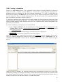
Once Sarra-H V3.2 is activated on your computer, every time you launch Sarra-H v3.2, you will see
the screen shown in the figure below (in alphabetical order, a folder of simulations appears, if it
already existed). You can display a folder of simulations of your choice (if it is already created) by
clicking on the button unfold of "Folder".
This is the Sarra-H modeling interface.
3
It should be noted that Sarra-H is actually composed of two functional parts: the user interface and
the simulation engine.
The user interface is the software that allows the user to "prepare" his/her simulations and launch
them.
The simulation engine function is to run simulations defined in the interface. This separation, that
gives full power to the model, was designed to enable third-party softwares to drive the simulation
engine. The same principle is used with R. We will discuss this part later.
In the user interface, a number of tabs are present. We shall distinguish the main tabs and their subtabs (each of which being attached to a main tab). There are five main tabs:
The "SIMULATIONS" tab: allows you to create simulations (defining the sites used, the
characteristics of the plots, crop characteristics, technical itineraries, and the observed data) and
realize them. The execution of simulations is performed from this tab, which has three sub-tabs:
o The "Creation and realization" sub-tab that enables to create, modify, delete and launch
simulations. At the bottom of the page that opens after clicking on the sub-tab, you have the
following buttons: "Create", "Modify", "Delete" and "Launch".
The "INITIAL CONDITIONS" tab: soil and ecophysiological characteristics of the crop(s) of
interest are predefined and configured in this tab. One can enter and set the characteristics of the
plot and soil, climatic zone (:
o The "Plot and soil" sub-tab for defining the type of soil and its physical characteristics with
respect to the water management;
o The "Climatic Zone" sub-tab that enables you to select and establish a link between Ids
(codes) of meteorological and rainfall stations to be used for simulations;
o The "Crops" sub-tab that allows to parameterize the model for a given crop/variety by
defining a range of parametric values whose harmony reflects the biological and
physiological characteristics of growth and development of the considered crop, in link with
the physico-chemical characteristics of the plot;
o The "Cropping practices" sub-tab that allows you to enter the sowing date, seeding rate, and
other parameters.
The "OBSERVED DATA" tab : allows entering and viewing PET data and observed data on the crop:
o The "PET Data" sub-tab allows to display and have access to the values of imported PET,
calculated by the model for a set of stations or a particular station;
o The "observed data" sub-tab allows you to view, enter or modify data observed on the crop
or the soil.
The "CLIMATE DATA" tab: allows you to view and manage rainfall and meteorological data
imported into Sarra-H and used during simulations.
The "RESULTS" tab: allows the exploitation of simulation data through a display interface in a table
or a simplified graph (graphical visualization of model outputs and comparison with the observed
data).
The menu bar consists of three items:
"Tools" item: provides access to a set of tools to facilitate data management in Sarra-H.
4
"Item?" allows access to the CIRAD website, report bugs and reaching the dialog box.
These tabs and menus are detailed in the appendix to this manual.
5
V Creating a country and a rainfall or a weather station
The use of Sarra-H tool requires at first the creation of the country and weather and rainfall stations
concerned by the simulations.
The procedure begins as shown by the figure below:
Click on "Tools", select "Countries and stations management" and "Helper for adding
Countries/Stations").
After clicking "Helper for adding Countries/Stations", a window is displayed as shown in the two
figures below:
To create a country, you must check out:
A country to the country list
The country is created by making a selection from a list of the five continents of the world and it is
defined by a code and a name.
6
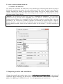
To create a station you must check out:
a station to the station list
The stations are created in the model with a more detailed geo-referencing that consists not only in
defining the continent, the country, the code and the name of the station, but also by specifying the
latitude, longitude and altitude of the location of the station. The type of station (synoptic station,
rainfall ...) must also be specified. Thus, after ticking on add a station to the station list; we get the
following window (Figure below):
Attention!!! It is written in the figure below (bottom): "bold fields are compulsory". This notification
doesn't need to be checked!! If the "longitude" box is not filled in, it creates a bug in the station
creation process. Whence, it is compulsory to fill in all fields in order to avoid the bug. It gives the
possibility to fill in the boxes (Latitude, Longitude and Altitude) in decimal degrees or degreesminutes-seconds (°, ' and "). In all cases, all the fields must necessarily be filled in to make it work. For
degrees-minutes-seconds, if there are no numerical values for the seconds ("), it will be necessary to
put "00".
VI Importing weather and rainfall data:
Climate data (rainfall and weather) must exist, at a daily time on a continuous basis for the period of
simulations. Before importing, the data must be saved in text format (. txt) within the Importation
folder of the DBEcosys of SARRA-H model. To reach Importation, you must click on:
7
C:\Sarra-H\DBEcosys\Import
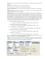
The import of weather and/or rainfall data is done by clicking on "Tools" in the SARRA-H interface.
A window appears and it shows two data import options: automatic data importation (figure below,
left) and manual data importation (figure below, right).
Figure 8A
Figure 8B
Automatic data importation
The automatic data importation is more convenient and it is not used only for weather and rainfall data.
It lets you import many types of data at once (by a single click): rainfall data, weather data, and
observed data from the plot/soil, crop, cropping practices and scenarios of simulations. However, for
the automatic data importation to succeed, it must be ensured that the data to be imported are saved in
Import, in formats required by the model. Indeed, the names of files to be imported into SARRA-H
should not have accents and their spelling should start (depending on case) by:
o Rainfall_ (+ name or code of the station), for rainfall data ;
o Meteorology_ (+ name or code of the station), for meteorological data) ;
o Folder_ (+ an Id), for a folder on a set of simulations
o SoilType_ (+ an Id), for data on soil characteristics
o ObsPlot_ (+ an Id), for data observed on crop in the plot
o Site_ (+ an Id), for data defining the weather and rainfall stations in the site
o Plot_ (+ an Id), for the soil type, surface thicknesses and soil depth defined for the
simulations
o Model_ (+ an Id), for the model used for simulations
o TechnicalItinerary_ (+ an Id), the technical itineraries data
o Simule_ (+ an Id), for scenarios of simulations
o Variety_ (+ an Id), for the variety characteristics data
o Etc,
NB: The import runs systematically for all text files (.txt) in the Import folder. So, if there are some
data (in Import folder) that you don't want to import, then they should be put in a subfolder, deleted or
compressed.
8
Also, particularly for meteorological and rainfall data, it must be ensured that the data column names
are written in the same way as originally foreseen in the model. The order of columns matters little in
SARRA-H, version 3.2. But spelling, case (uppercase, lowercase) and spaces after the column titles of
the file to be imported shall strictly comply to those indicated below:
-
CodeStation, Day and Rain, for rainfall data ;
-
CodeStation, Day, TMax, TMin, TAvg, HMax, HMin, HAvg, Vt, Ins et Rg, for meteorological
data.
Attention! To avoid bugs, don't add measurement units (mm, ° C, %, m / s, etc) in the columns names
of weather and rainfall data that you wish to import.
We must also ensure that the decimal symbol (dot or comma) used for the data to be imported is the
same as that selected in the computer (start Control panel Regional options Customize Decimal symbol and choose the same decimal (point or comma) as for the file(s) you wish to import
into SARRA-H). The change of decimal symbol may also be done in the SARRA-H model by using
manual importation of data option (see next chapter).
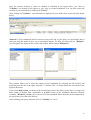
The figure below shows an example of data files ready to be imported automatically into SARRA-H
model, after clicking on: Tools and automatic data importation.
9
Manual data importation
The manual data importation can also be used to import various types of data into the SARRA-H
model: Climate data (rainfall and meteorological), irrigation, data observed on crop and the model's
forcing data. When you click on Tools
and then manual data importation, a
window is displayed as shown in Figure A
(above). This window shows (top left)
that the manual data importation involves
three (3) successive steps: (1) Connection
(2) Association (3) Execution.
1) Connection step: This tab gives access
to data to be imported by using one of the
following access options: "Select File ..."
(top left) and "Paste data" (top right)
a) "Select file ..." provides access to the
data file you wish to import from a
directory where it is stored in the
computer, by using the classical
procedure for opening folders and files
with Windows Explorer. Once the data
file to be imported is reached, just click
on the file (txt. format) and then click
Open and the data is displayed in the box
provided for this purpose in the import
window as shown by the Figure B (above)
(an example for rainfall data).
A
B
b) "Paste Data" This option gives the
same visualization of the data to be
imported as in Figure B, by copying and
pasting the data directly in the window
provided for this purpose. But, be
careful!!! this operation cannot be
performed on too many data :
- Open the data file to be imported,
select all the data (with column names),
then click on copy ;
C
- Go into SARRA-H, click Tools,
manual data importation and then click
paste data. The data pasted into the open
window are displayed as shown in Figure
C. The importation should then be
validated by clicking on accept (bottom,
right of the window).
This second data access option to manual
importation has the advantage of enabling
to use not only data stored in text format
(txt.), but data in Excel format.
2) Association Step: it comes after the
connection step. It helps establish a
10
matching link between column names assigned to data to be imported and those initially provided in
SARRA-H for the same data types. This procedure of association allows bypassing respect constraints
for the columns names spelling in the case of an automatic data import.
To perform the association, you must click on 2-Association, then select in the window that opens,
type of data to import (see figure in
left). Once we have ticked the type of
data to be imported, the model gives
(through sub windows that open
gradually, the opportunity to choose
the continent, country and the station
concerned
by
the
envisaged
simulation or simulations.
The association is made by selecting,
each time in the two named columns,
your file and DBEcosys (figure
above), the couplet of similar
parameters and by clicking on <Association-> (see in between
columns, your file and DBEcosys
(Figure above)).
Once this is done, the association's
result appears in the Result column (figure above, right). This exercise of association by
correspondence is done for all parameters whose names appear both in the two columns; your file and
DBEcosys. Once associations completed, proceed to Step 3
3) Execution step: this is the last step of the manual data importation. It requires little manipulation.
Just click on 3-Execution (top) then click on Import (bottom) for running the data importing process
as shown in the figure below. However, the figure doesn't show an example of a complete process of
data import. For realizing it, we must read what is written under the figure:
ATTENTION - ATTENTION - ATTENTION
This is an update test because the "Update test or Add test" box is checked
NO DATA HAS BEEN WRITTEN IN DBECOSYS
Indeed, this is just a test
(optional) of update or import.
To run the definitive data
importation, you have to
uncheck the Test box before
11
updating or adding (to the top left of the figure cons), then click on Import (this can be done without
going through the update Test). One can verify the effectiveness of the importation in the Importation
Result sub window (figure cons) before leaving the manual data importation window.
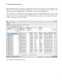
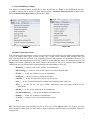
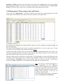
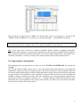
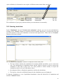
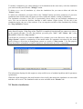
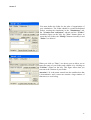
VII Management of Meteorological and rainfall data:
Click on the tab "Climate Data". It enables to display at the same time, meteorology data (in a table
on the right) and rainfall data (in a table on the left), as shown in the figure below.
By selecting the continent, the country then the station, you can visualize the desired rainfall and
meteorological data.
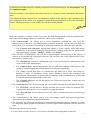
The input field "Filtering the year" makes it possible to quickly have a view on a given year. To stop
the process of year's filtering, click the button named: [Filter].
At the bottom of the window, there are two sub-tabs: "Switch to modification mode" and "Chart". The
"Switch to modification mode" sub-tab is used to display and manage (modify or enter) meteorology
and rainfall input data that can be used for simulations.
Indeed, the data grid is by default in read only mode. This functionality becomes useful when you spot
an outlier. It also allows you to force a climate value, manually. When you click on this button, it is
renamed [Skip in consultation] and an alert message warns you when you switch to modification
mode. The SARRA-H platform’s environment turns into light blue (see figure below).
Note: note that any modification/deletion is
saved immediately in the DBEcosys
database and no backtracking is possible. It
is therefore important if you wish to modify
temporarily these data that you take note of
changes made manually, so that you can
reenter the original values.
To return to the normal mode, consultation
mode, click [Switch to consultation].
12
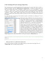
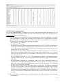
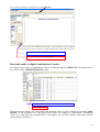
VIII Calculating PET and Verifying Climate Data
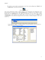
The verification may be made by updating the ETo balance sheet. To achieve this, click on "Tools", a
window will display, and select "Regenerate the calculated ETo". A window (see figure below) will
open. This window shows that it is possible to update the ETo: "for all the database", a given
"continent", "country" and/or "station". The procedure consists of selecting the button corresponding
to what one wants to do, among the four listed (4) options. After making your choice, the boxes
"Continent", "Country" and/or "Station" (figure below) are activated (according to cases) for you to
choose the continent, the country and/or station for which you wish to verify climate data through the
ETo update.
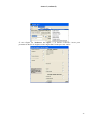
It is only after these steps that you can launch the update (verification) by clicking the "Execute
Update" button (figure below).
During this update, SARRA-H will explore the content of
your climate database to verify if data contained in your
climate base allow the calculation of evapotranspiration
(reference evapotranspiration, FAO procedure-PenmanMonteith called FAO 56 - ). At the end, it will analyze the
data and verify their presence over the concerned year.
Indeed, the ETo procedure recommended by FAO, requires
having minimum and maximum (or average) temperature,
minimum or maximum (or average) relative humidity of
wind and global radiation (or sunshine duration). If for a
given year, the data is missing, the display for the year in
question will be in gray. If one single data (eventually for
one single day) is missing within the concerned year, the
display of the year in question will be in red. If all the
necessary data are present, the display will be in green (see
example figure below). This information box is always present in the "Climate Data" tab.
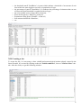
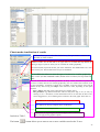
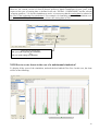
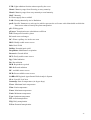
Other procedure for a rapid check of climate data
The procedure consists in clicking on the "Chart" button (see the bottom of the figure above, in
"Climate Data" tab). A window opens as follows:
13
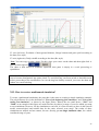
This tool allows visualizing quickly and graphically the consistency of your data for the selected
station.
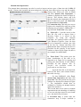
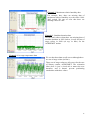
Example 1: Maximum temperatures data:
This figure shows that there is no missing data for Tmax (for the AGRHYMET station) over the 19912007 periods. For example, if there are empty records (missing data) the corresponding period is
marked by + + + in red. If there are out of range values (excessive temperature and/or outliers notified
by the model which nevertheless takes them into account as such in the simulations), the
corresponding period or day(s) are marked by + + + in blue. For the existing and valid values, they are
always marked by + + + in green.
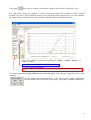
Zoom: The chart can be zoomed quickly. For this, click with the left mouse button on the chart and
hold it, then move down and to the right. It draws a rectangle. When you release the mouse, the chart
will zoom in on the area included in the rectangle
To stop the zoom, click and hold on the click and move the mouse to the left and upward.
By zooming for a certain number of times, one can
visualize the exact dates of out of range or missing
values (figure on the left).
To zoom, click to the area you want to enlarge.
Make a rectangle from top to the bottom from left to
the right and release the button. The zoom will
appear.
To "unzoom", click on the graph from bottom to the
top, from right to the left.
14
Example 2: Maximum relative humidity data
For example, here, there are missing data of
maximum relative humidity over the entire 19942003 period. We can see also that there are
missing values in 1990.
Example 3: Sunshine duration data
We can easily observe that there was missing data of
sunshine duration in 2002 (below, in red) and out of
range values in 2000 (on top, in blue) for the
AGRHYMET station.
Example 4: Average temperature data
We see that these data are all correct although there
are out of range values (in blue).
These out of range values are all correct for the case
of Niamey station, AGRHYMET. The coloration
(bleu) here is just a visual aid to attract the user
attention, and it doesn't prevent performing
simulations with these values.
15
IX Climate data exportation
To export climate data, you must first display the station you want to recover data (e.g. the
AGRHYMET station in the figure below).
Once the station is selected, you have to click on "export" (see A on figure below):
B = this pop-up window allows you to select the type of data you want to export (rainfall data,
weather, observed data of a country, station, etc.)
C = this pop-up window allows you to specify the station (station code) you want to export the data.
D = when this button is checked, it allows you to export the data (depending on type) of a continent, a
country, stations or folder. When it is not checked, you can select within the window (press Ctrl for
multiple selections) the type and / or data set you want to export.
E = this button allows you to execute the exportation
F = press this button to exit the action
A
B
C
D
E
F
Once the station is selected, you need to choose what types of data should be exported (meteorological
data, rainfall, observed data, etc...).
Once the export is launched, another small window opens as shown in the figure below; to give you
the possibility of assigning an Id for the file you want to export. This Id (10 characters in maximum),
is always preceded by another Id automatically displayed by the model, depending on the type of data
(meteorology, rainfall, ObsParcelle (data observed from the plot), etc...).
16
After giving the Id, then click on "OK", the exported data can be recovered (in txt. format) in the
"Export" folder of DBEcosys. To get there, you must go through C: \ Sarrah\DBEcosys\Export.
Important Note: You cannot export rainfall data and meteorological data directly by selecting both at
once. This must be done separately, that is, one single exportation for each data type.
NB : In the same way, can also be exported simulation folders (Folder), simulations (simulate),
simulation results (Resjour), site data (Site), information on the plot (Plot), irrigation data (Irrigation),
data of technical itineraries (technical itineraries), the observed data (ObsParcelle), information on a
continent (Continent), a country (Country) and a station (station) with all their characteristics).
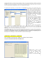
X Crop parameter management
The management of crop parameters is carried out via the "INITIAL CONDITIONS" tab and sub-tab
"Crops".
The sub-tab named "Crops" allows you to view and modify plants characteristics used during the
simulations. It consists of a grid of organized data in the form of parametric values, defined to take into
account the different physiological and environmental factors that govern the growth and development
of cereal varieties. The parametric values enshrined in the grid (figure below) are used to calibrate the
SARRA-H model for different varieties, and each according to its own physiological characteristics
(phenology, biomass accumulation, allometry, etc...). During calibration and model simulations, some
parameters may vary depending on the species and varieties, but others may still remain invariable,
especially for varieties of the same species.
17
XI Soil texture management
The sub-tab "Plot and Soil" is composed of a grid of data representing the characteristics of soil
textures usable during simulations. When you click on the sub-tab, a window opens and displays two
complementary tables, as shown below:
1) The first table is used to define the textural characteristics of the soil (soil typology), in relation
with its capacities to contain water according to two depth levels: a superficial level (surface
reservoir) and a level of depth (depth reservoir covering the soil portion that can be explored by
the plants roots). This table enables defining (by typing) :
o the soil Id (Id), (1st column),
o the soil name (2nd column),
o the stock of soil water usable by the plant in the superficial level (3rd column), at sowing (it is
considered as null (0.00) for seedlings without roots (seeds), but must have another value >
or = 0.00, in link to the level of soil moisture for transplanted crops having roots for water
tapping from the soil, at the outset),
o the stock of soil water usable by the plant in depth (4th column), at sowing (it is considered as
null (0.00) for seedlings without roots (seeds), but must have another value > or = 0.00, in
link to the level of soil moisture for transplanted crops having roots for water tapping from
the soil at the outset),
o the soil thickness favorable for the soil evaporation on surface "EpaisseurSurf (mm)"
(generally fixed at 20 cm ( 200 mm for typing into the model) for sandy soils and less for
clay soils),
o the soil thickness containing the consumable water by the plant "EpaisseurProf (mm)". It
represents the soil depth achievable by the plant roots. For cereals, it can reach 2 m (2,000
mm) in the case of sandy soil and below when it comes to a clay soil texture. For a soil depth
of 1.8 m, we will consider 1,800 mm,
o the last column is not reserved to any manual process of data input, but it allows establishing
a link (by correspondence) with the complementary information registered in the 2nd table
below, for each soil type. For this, we must make two separate clicks (different from doubleclick) in the box corresponding to the selected soil type. A scrollable window will appear to
allow you select the Id of complementary characteristics of the soil type that is located in the
2nd table.
2) The second table (complementary to the first) indicates the values assigned to the following
soil parameters :
18
o the threshold runoff "SeuilRuiss" (in mm) which indicate a threshold of an amount of rain
from which the water begins to run off on a particular soil type,
o the percentage of runoff "PourcRuiss" (%) indicates the percentage of rainwater that can run
off once the runoff threshold is reached on the soil type,
o the soil available water content (RU) (in mm/m),
o Water field capacity « HumCR » of the soil,
o Permanent wilting point « HumPF » of the soil,
o Soil moisture threshold « HumSat »,
o etc.
XII. Creating a site
To create the site, it is necessary to have rainfall and meteorological stations already created in the
Sarra-H model. It is created by clicking on the tab "Initial conditions", then on "Climatic Zone" subtab. After the clicks, we get the following window:
19
-
In the "Id" column, you must enter the Id (name) of your site (eg "Alka", as in the figure
below);
-
In the "KPar(MJ/MJ)" column, enter the default value 0.50, which corresponds to the
proportion of the photosynthetically active global radiation;
-
In the "Ref_CodeStationPluie" column, click twice (not double click, but two separate clicks)
in the Id line (name) that you have just entered. A scrollable window appears as in the figure
below, to allow access to the code of your rainfall station. Unroll, by clicking on the arrow to
select the code of your rainfall station.
-
In the "Ref_CodeStationMeteo" column, as for the rainfall station, click twice in the same
line. A scrollable window also is displayed to allow access to the code of your meteorological
station. Unroll, by clicking on the arrow to select the code of your meteorological station as
follows:
Attention!!! If you just create your rainfall and meteorological stations, you can find their codes in the
scrollable windows "Ref_CodeStationPluie" and "Ref_CodeStationMeteo" only by closing
necessarily Sarra-H and reopen it (Sarra-H saves your changes systematically anytime you close it).
Also, the current version of Sarra-H V3.2 allows you to modify a site already created, but it does not
allow you to delete it (even in case of error)!!!
Once this is done, you have finished creating your Site.
The "Climatic Zone" window also provides access to the direct management of stations/countries and
to adding country/station, by clicking, according to the case, on one of the following buttons: "Direct
management of stations/country" and "Assistant for adding country/station" (see the figure
below, right).
20
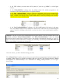
XIII. Creating a simulation
Sarra-H is a crop model software. The exploitation of this software is based primarily on a stream of
input data from a database named DBEcosys. Current data (ecophysiological characteristics,
declaration from the cropping site, the plot, technical management ...) as well as climate data are
hosted in this database. The DBEcosys relies on a local type of database management system, located
on your hard drive. Thus, as already mentioned above, the Sarra-H model saves systematically data
that are modified, imported or entered by the user.
To perform a simulation, this model requires a certain number of input parameters (climate data, data
characterizing the crop, the site, the plot ...). As already noted above, rainfall and meteorological data
must exist in the Sarra-H model, on daily time series, on a continuous basis which corresponds to the
period of your simulation.
To create a simulation, you must have previously defined:
In the "Initial conditions" tab: the characteristics of the plot and soil, the cropping site (in the
"Climatic Zone" sub-tab), ecophysiological characteristics of the crop (in the "Crops" sub-tab)
and cropping practices;
Climate data (rainfall and meteorology) collected from your cropping site;
Observed data, for eventual comparisons with model outputs.
Once the environment is characterized, just create your simulation (period x model x site x plot x
variety x technical management (observed data being facultative)) in the "Simulations" tab, the
"Creation and realization" sub-tab and the "Create" button (see in the corner, down the figure
below).
When you click on "Create", the following window opens systematically to allow you to create your
simulation by linking (by selecting as shown by the blue bands in the figure below) the parameters that
you already defined for your plot, your site, your variety, your technical management and the type of
model you want to use. In that same window, you must also define:
21
-
Plot : Select the plot attached to the declared Site above, on which you want to launch the
simulation;
-
Model: Select the model you want to use for the simulation;
-
Site : Select the site on which you want to launch the simulation;
-
Technical management: Select your plot technical management (sowing date, sowing density,
etc.);
-
Observed data: choose the observed data on your crop with a view to compare them with the
model simulations (their choice is optional)
-
Simulation dates: the year of the beginning first simulation and the year of the ending last
simulation must be in the format [yyyy]. For the beginning of the cropping period and the end
of the cropping period, they must be in the format dd/mm. These dates correspond to the
beginning and the end of the simulation. The fields format [yyyy], enables you to use Sarra-H
for simulations on a multiannual period. In the case of a mono-annual simulation, these fields
must be identical, as shown in the figure below. In the case of a multiannual simulation, these
two dates are generally situated on the same year for the northern hemisphere and on two years
maximum for the southern hemisphere. Here is a sample of chronological configuration:
•
Annual Simulation, northern hemisphere:
o First cycle: 15/05/2004 to 31/10/2004, Simulation year (s): 2004 to 2004
•
Multiannual Simulation, northern hemisphere:
o First cycle: 15/05/2004 to 31/10/2008, Simulation year(s): 2004 to 2008
•
Annual Simulation, Southern Hemisphere:
o First cycle: cycle : 15/10/2004 to 31/05/2005, Simulation year(s): 2004 to 2005
•
Multiannual Simulation, Southern Hemisphere:
o First cycle : 15/10/2004 to 31/05/2008, Simulation year(s): 2004 to 2008
•
Simulation of perennial crop :
o First cycle : 15/05/1950 to 31/10/2008, Simulation year(s): 1950 to 2008
-
Id (= your simulation name), it must characterize the simulation that you will create (see the
bottom of the figure, below: Simul_Alka_2004, for example);
-
Folder: it allows you to create a virtual folder in which your simulation (s) will be hosted. By
selecting a folder (in the dropdown list, only simulations defined in this folder will be
displayed. Further details are given on creating folder in Appendix 2.
22
Once the various elements or items are defined as indicated in the figure above, you click on
"Validate" (see bottom of the figure) to save your so created simulation. You can also cancel the
creation of your simulation by clicking on "Cancel".
After clicking on "Validate", your simulation is displayed in your folder sheet, as shown in the figure
below.
Attention!!! Your simulation doesn't execute as long as the Ids of your query are not defined, that is
what you want the model to give you as simulation outputs. For this, you must click on "Redefine"
(see top right of the figure above) to have the window below named "FRequetes".
This window allows you to select the output of your simulation by selecting into the left box and
displacing into the one at the right, using the ">" button. The "<" button allows the movement in the
opposite direction.
If you select Daily results, as shown in the second figure below, this allows you to have, as output, the
daily results (in digital form visualizable in graphical form) of the simulation about the biomass
evolution. "Biomasse_récolte" gives you access to the simulated values about the yield components at
the end of the cycle; that is the harvest.
After defining your query elements, click on "Validate" to save it.
23
Après validation, les éléments de votre requête s’affichent comme montré dans cette figure
This redefinition of your query elements allows your simulation to run normally.
XIV. Running simulations
In the "Simulation" tab and "Creation and realization" sub-tab, you can run your simulation by
clicking on the "Launch" button (see bottom of the left column). But before, you must first click into
your left column to select your simulation, as shown in the figure below. Then, click on "Launch"
(bottom of the same column)
The "Creation and realization" sub-tab is composed of three main parts:
•
The left column contains the simulations list already defined and allows you to create new
ones. The management of simulations names and the folder to which you wish to connect the
simulation is also done at this level. It is also possible to delete, modify or export the
simulations at this level (we'll talk about it later).
•
the right part allows to display the parameters used by the simulations,
•
The top box, where the redefined elements for the simulation query are displayed.
To launch a simulation or a set of predefined simulations, select the desired list of simulations and
click the "Launch" button.
24
To modify a simulation (you cannot modify several simulations at the same time), select the simulation
you want to modify and click the "Modify" button.
To delete a (or a set of) simulation (s), select the simulations list you want to delete and click the
"Delete" button.
To add a new simulation, you must click on the "Create" button and select parameters of your new
simulation in the window that will appear (see above under the subtitle, creating a simulation).
The simulation execution is fast, but it is particularly slower when you run multiple simulations at
once. You can see that the interface launches a small window (Figure below). In fact, this is the
simulation engine, the core of the software. You can stop the execution of the simulation by clicking
the "Stop simulation" button.
Attention!!! Attention! When you stop ongoing simulations, most often a bug occurs and it blocks the
entire Sarra-H engine. If this bug occurs, Sarra-H is completely blocked and you cannot even close it
by the normal procedure. To solve the problem, you must press "Ctrl" "Alt" "Delete / del", select
Sarra-H-V3.2 and click "Stop session".
It will then be necessary to relaunch SARRA-H to continue your work. But more often, this action
"Stop Session" requires a compacting of the model tables for automatic correction (by the model
itself) of bugs or errors into its management system as a result of "End session ". For this purpose,
when the model is relaunched, a window displays to warn about the need for a compacting.
The information displayed in this engine are only useful in case of technical problem and for parameter
optimization.
When the engine disappears (the small window closes itself), that means the simulation was successful
and there was no error. The simulated results are now available in the "Results" tab
XV Results visualization
25
Pour visualiser les résultats, il faut cliquer sur l’onglet "Résultats"
Il y a deux options de visualisation des résultats : option numérique et option graphique.
Pour passer d’une option à une autre, il suffit de cliquer sur l’un des boutons suivants :
Ici, pour visualiser les résultats numériques
Ici, pour visualiser les résultats graphiques
Data table mode or digital visualization of results
The figure below shows a visualization of observed data through the "RESULTS" tab (data can also
be viewed via the "OBSERVED DATA" tab).
La procédure consiste à :
- Sélectionner "Données observées", dans cette case déroulante
et à
- cliquer sur ce bouton
With the same procedure, one can visualize the simulated values (for all variables) by selecting "Daily
Results" in the scrollable box. The figure below shows an example of visualization of simulated
values. As visible from the scrollable box in this figure, one can also visualize other types of data
(meteorology, rainfall etc.).
26
Charts mode visualization of results
This box allows you to select the simulation (s) that you wish to visualize the
data table or chart result(s)
This box is a filter/year. It allows you to select the year for which you want to visualize the
simulation results. On the left and to its right, there are 2 fields that help define (by
entering) a range of years for which you can visualize the results graphically.
The first field (left) represents the first year of the simulation. The middle field is the chart
of the current year. The last field is the last year of simulation
This scrollable box allows to select the types of results to be visualize graphically:
Daily results (for the simulated results) and/or Observed data (for crop observed
data) :
This box shows the list of simulated parameters (in Daily results) and observed parameters
(in Observed data) that one can visualize graphically. One can visualize the evolution of one
or more parameters, according to Julian days (see Day, in the box below cons) and the
number of days after sowing (see Nbjas in the same box). Thus, depending on the option
selected:
- Day or Nbjas, then slide in the X box(X-axis) by clicking "X>";
- The parameter (eg BiomasseAérienne and/or Yield), then drag in Y1 (Y axis), by
clicking on "Y>". Parameters, whose measurement unit is not the same as those of Y1,
can be dragged in Y2, for visualizing their evolution in the same graph. Then click on:
This button, for visualizing the chart
This button, for moving to digital values visualization
This button, for erasing the chart
This button, for exporting the simulations digital values on Excel (this
does not apply for the graphics option).
Just below "Y2>",
The button
button allows you to remove one or more variables used on the Y axes.
27
The button
allows you to remove (clear) all the variables used for the X-axis and Y-axes.
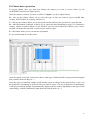
The chart below shows an example of a chart visualization about the evolution of above ground
biomass (red curve), the leaf biomass (green curve) and grain yield (yellow curve). For each variable,
the points represent the observed values and the continuous lines, the simulated values.
Pour choisir l’option de représentation graphique en "Points", "Lignes", "Barres", ou
"Aire", il suffit de :
- Sélectionner la variable dans la liste Y1 ou Y2
Puis dans "Style des graphiques"
- cliquer (selon le choix) sur "Point" (point), "Line" (ligne), "Bar" (barre) ou "Area" (aire)
The button group named type of charts allows determining the chart type to be applied to one or more
variables.
For this, simply select from the list Y1 or Y2, one or more variables (hold down
the Ctrl button), then click on the desired type. The graph is redrawn immediately.
28
Y1 axis (left axis): Evolution of aboveground biomass, foliage biomass and grain yield according to
the date (Line style).
Y2 axis (right axis): Daily rainfall according to the date (Bar style)
Note: You can copy or print a chart. For this, place your cursor on the chart and then right click. A
shortcut menu appears:
The chart is then stored in Windows clipboard, then paste it simply in a word processing or
spreadsheet.
Attention!!! When you are in chart visualization mode, if you modify an observed value, the chart
curves become disorganized into points cloud. To avoid this bug, one must switch to data table mode
before proceeding to the modification. In case the bug has already occurred, just erase the chart and
redraw it to correct the bug.
XVI. How to create a multiannual simulation?
To create a multiannual simulation, the procedure is the same as creating a simple simulation (annual).
The only difference lies in the definition of "Year of the beginning first simulation" and "Year of the
ending last simulation", as shown by the figure below. Indeed, the two small boxes; "1961" and
"2000" as an example in this figure are used to define (by choice) a range of years for which you want
to run simulations. However, for the simulations to succeed, it is first necessary to have in the Sarra-H
model; meteorological and rainfall data for the entire selected years range. The results of these
simulations are annual, and one cannot, for now, directly get one single simulated value, for a whole
considered range of years.
29
Attention: multiannual simulations work well for years following the year of the sowing date.
However, the current version of Sarra-H doesn't permit to launch simulations for past years, with
respect to the year of sowing date as defined in the tab "INITIAL CONDITIONS" and the sub-tab
"cropping practices ". So for the simulations to work, it is necessary that the sowing date be reduced to
the year of the beginning first simulation!!! For example, for launching multiannual simulations over
the period 1961-2000, it would be necessary to have the sowing date in 1961.
Define here (in format aaaa),
The year of the beginning first simulation
and
The year of the ending last simulation
XVII How to create charts in the case of a multiannual simulation?
To display all the years of the simulation, uncheck the box labeled Filter/Year. In this case, the chart
will be as the following:
30
Annex 1
-
The modeler version, which is complementary to the User version (adding items "Models" and
"configuration" in the Sarra-H menu bar).
SarraH_3_2_modelisateur.exe
Only persons authorized to make or suggest changes in the management and configuration of the
Sarra-H model are provided with the version modélisateur.exe. To install it in your computer, simply
double-click the modélisateur.exe and follow the instructions on the screen. This version
(complementary to the previous one) simply allows to have access and to use "Models" and
"Configuration" items (which don't appear in the user Version), as shown in Figures 1 and 2. (See
Annex x.x)
Si vous cliquer sur "Gérer…", la fenêtre ci-dessous s’ouvre pour permettre l’accès au module, au
modèle, aux librairies et unités et aux rapports.
31
Annex 1 (continued)
Si vous cliquer sur "Ordonner les onglets…", la fenêtre ci-dessous s’ouvre pour
permettre de choisir les onglets et sous-onglets dans l’ordre que vous voulez.
32
Annex 2
You must define the folder for the sake of organization of
your simulations. The folder should be created beforehand
(before creating the simulation) in the "Simulations" tab,
the "Creation and realization" sub-tab and the "Folder"
checkbox (figure on the left): the "New" button allows to
create the new folder, the "Modify" button to modify it and
"Delete", to delete it.
When you click on "New", two boxes open to allow you to
enter the name of your folder and validate it by clicking on
"Validate" (Figure on the left). This figure shows that you
can cancel the creation of your folder.
Attention!!! It is the name entered into the smallest box that
is determinative and it must not contain a large number of
characters, to avoid a bug.
33
Annex 3: ACRONYMS AND ABBREVIATIONS USED IN SARRA-H
Biomfeuille: Leaf biomass
Biomgainj: Daily gain in biomass
Biomtot: Total biomass
BiomTotStadeIp: Biomass at the panicle initiation stage
BiomtotStadeRPR: Biomass at the flowering stage
BVP: Basic Vegetative Period
CSTR: Stress Constant
DayRdt: Daily yield
DayRdtPot: Potential daily yield
εb (Epsilon b) : Conversion efficiency of intercepted radiation to dry matter
ETM or ETRM: Maximum Evapotranspiration
ETo: Reference Evapotranspiration
ETR: Actual Evapotranspiration
EvapPot: Potential Evaporation
EVj : Daily Evaporation
FESW: Fraction of evaporable soil water
FTSW: Soil water transpirable fraction
HI: Harvest index
IRESP: Expected yield index
JAS: Days after sowing
K: light extinction Coefficient
Kbasefeuille: Basis of the relationship between above ground biomass and leaf biomass/above ground
biomass
KC: crop coefficient
KCE: Part of the crop coefficient due to soil evaporation
KCMAX: Maximum crop coefficient
KCP: Part of the crop coefficient due to plant transpiration
Kmulch : Coefficient of soil roughness
KPar : coefficient of photosynthetically active radiation (Kpar = 0,48 à 0,5)
Kpentefeuille: slope of the relationship between (leaf biomass/above ground biomass) and the above
ground biomass
kRdt: Potential yield evaluation coefficient from the difference of biomass between the flowering and
the panicle initiation stages
Krealloc: Reserves reallocation coefficient
LAI: Leaf area index
34
LTR: Light radiation fraction unintercepted by the cover
Matu1: Maturity stage from flowering to waxy maturity
Matu2: Maturity stage from waxy maturity to total maturity
MAT: Maturity
P: Water supply due to rainfall
PAR : Photosynthetically Active Radiation
parP: Specific Parameter to each species which expresses the soil water critical threshold at which the
water stress reduces linearly the plant transpiration
pF4: Wilting point
pFactor: Transpiration rate calculation coefficient
PSP: Photoperiod-sensitive phase
R: lateral water exchanges
RC: Water capillary rise in the root zone
RDU: Hardly usable water reserve
Rdt: Grain Yield
RdtPot: Potential grain yield
RespMaint: Maintenance respiration
Restcrois: Growth deficit
RFU: Easily usable water reserve
Rg: Global radiation
Rn: Net radiation
RPR: Reproductive period
RR: Reflected radiation
RU: available water reserve
RUR: Root available water reserve
SARRA-H: Regional Agroclimatic Risks Analysis System
SLA: Specific Leaf Area
Somtemp: Sum of temperatures (in degree days)
Tbase: Minimum basic temperature
Tlim: Limit temperature
Tmax: Maximum temperature
Tmin: Minimum temperature
Topt: Optimum temperature
TR: Actual transpiration
TRj: Daily transpiration
TrPot: Potential transpiration
35