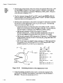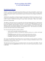
1
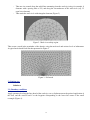
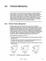
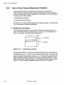
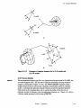
Fracture problems with ANSYS
A (very) brief introduction
Introduction and objective
ANSYS is a commercial finite element code used in industry to solve large scale problems. It can be used
to solve a wide variety of problems including linear and nonlinear structural response, buckling, modal
analysis, full harmonic response, transient dynamic response, heat transfer, electro-magnetic and fluid flow
problems.
ANSYS offers a large library of elements ranging from the simplest (1-D elastic bar element) to the very
complicated (3-D nonlinear elasto-plastic element). Information about these elements and the type of
analysis available in ANSYS can be found in various sources and manuals. Help is also available
interactively within ANSYS.
The objective of this short exercise is to extract the value of the stress intensity factor for a compact tension
test (CTT) linearly elastic specimen described in Section A4 of the E 3999 ASTM Standard (see first two
pages of the Appendix of this document). Basically, we want to perform a 2-D structural analysis with
ANSYS to extract in an automatic fashion the value of the stress intensity factor for various crack lengths
and reproduce the results indicated in Equation (A4.1) and Table A4.5.3.1. This will allow us to assess the
precision of the finite element code for fracture problems.
We will use the following utilities available in ANSYS
- log files used to run similar simulations automatically,
- scalar parameters definition, to automatically change the specimen size w and the crack length
a,
- the KSCON command, which allows to generate focused mesh at the crack tip,
- the “skewed element” option, used to generate singular elements at the crack tip
- the KCALC command used to extract the value of the stress intensity factors
The section of the ANSYS Procedures Manual relative to the simulation of fracture problems is included in
the appendix of this document. Please spend a few minutes reviewing the information relative to 2-D
fracture analyses on pages 3-156 to 3-160.
The following lines describe the series of commands needed to solve the problem with ANSYS. The pick
commands are denoted by regular bold words, while values to be entered (using the keyboard) are given
in italic bold.
1
Problem description
The structural problem to be solved is described in Figure A4.1 of the Appendix. Taking advantage of
symmetry and simplifying the geometry a little bit, we will actually solve the following problem:
To prevent rigid body translation, we will fix the x-displacement of the point of application of the load P.
To facilitate the creation of the focused mesh at the crack tip, we will place the origin of the axis system at
the crack tip.
The material properties will be chosen as those of PMMA (E = 4000 N/mm2 and ν = 0.3), although, for this
problem, the material properties do not enter the expression of the stress intensity factor. The load P will
be chosen as unity. We will perform the analysis in plane strain.
ANSYS analysis
This session assumes some familiarity with ANSYS. Only the steps specific to the fracture analysis will be
described here. The other steps are identical to those of a conventional plane strain structural analysis.
1) Preliminary steps
Specify new job name (optional) and new title (optional).
Under the heading Parameters, define the two scalar parameters
w=100
a=0.45*w
Select Structural under Preferences… (optional)
2) Preprocessing step
Preprocessor >
2
2.1) Element and material definition
We will use 6-node triangular elements (Plane2). Make sure to select the plane strain option.
No real constant definition is needed for this type of element
Define a material set (Constant-Isotropic) with the appropriate properties (stiffness and Poisson’s ratio).
2.2) Geometry definition
The easiest way to define the geometry is to define
- a semi-circle of radius a/5 centered at the origin
- a large rectangle (xmin=a-w, ymin=0, xmax=a+w/4, ymax=0.6*w)
- a small rectangle (xmin=a, xmax=a+w/4, ymin=0.275*w, ymax=0.6*w
Then use the Operate/Overlap/Areas action to subtract the two smaller surfaces from the large rectangle
(Figure 1).
Figure 1. Definition of areas, lines and keypoints.
2.3) Mesh generation
First create the mesh in the semi-circle:
- First, create a concentrated mesh at the crack tip with Mesh-Size Control-Concentrated
Keypoint
Pick a/20 as the radius of the first circle
Pick 1.5 for the radius ratio (2nd row/1st row)
Use 5 or 6 for the number of elements around the circumference
Use the Skewed 1/4 pt. option for the midside node position
3
-
Then use size control along the radial lines emanating from the crack tip (using, for example, 8
elements with a spacing ratio of 2,5) and along the circumference of the semi-circle (say, 12
equal size elements)
Then mesh the semi-circle with triangular elements (Figure 2)
Figure 2. Mesh in crack tip region.
Then create a mesh in the remainder of the domain, using the mesh tool and various levels of refinement.
A typical mesh should look like that presented in Figure 3.
Figure 3. Full mesh.
3) Solution step
Solution >
3.1) Boundary conditions
Apply symmetry bc along the line ahead of the crack tip, zero x-displacement on the point of application of
the load, and the vertical load P at the keypoint corresponding to the lower left corner of the small
rectangle (Figure 4).
4
Figure 4. Boundary conditions
3.2) Solution
The solution should take just a few seconds.
4) Post-processing
General Postproc >
4.1) Deformed shape and stress concentration
Contours of the σyy stress distribution should clearly indicate the presence of a stress concentration at the
crack tip (Figures 5 and 6)
Figure 5. Deformed shape and stress distribution.
5
Figure 6. Stress distribution in the crack tip region.
4.2) Extraction of the SIF
As explained in the appendix, we must first define a path in the vicinity of the crack tip. But before doing
so, we must define a new coordinate system “pointing ahead of the crack”, using the following command:
Work Plane / Local Coordinate System / Create Local CS / By 3 Nodes
- pick the origin first (crack tip node)
- then pick a node along the new x-axis (i.e., a point along the plane of symmetry)
- finally, pick any node in the new x-y plane (i.e., any node off the plane of symmetry)
After defining the new CS, let us define a path with
Path Operators> Define Path> By Nodes+
Then pick successively three nodes behind the crack tip (i.e., along the crack face), with the first one at the
crack tip, the second close to the crack tip, and the third one a little further away (you can pick the first
three nodes if you want).
Finally, extract the stress intensity factor with Nodal Calcs> Stress Intensity Factor, which will create a
separate window with the following information:
****
CALCULATE MIXED-MODE STRESS INTENSITY
FACTORS
****
ASSUME PLANE STRAIN CONDITIONS
ASSUME A HALF-CRACK MODEL WITH SYMMETRY BOUNDARY CONDITIONS (USE 3 NODES)
EXTRAPOLATION PATH IS DEFINED BY NODES:
WITH NODE
26 AS THE CRACK-TIP NODE
26
36
37
USE MATERIAL PROPERTIES FOR MATERIAL NUMBER
EX =
4000.0
NUXY =
0.35000
1
AT TEMP = 0.00000E+00
PRINT THE LOCAL CRACK-TIP DISPLACEMENTS
CRACK-TIP DISPLACEMENTS:
UXC = 0.11685E-02 UYC= 0.00000E+00
NODE
26
CRACK FACE
TIP
RADIUS
0.00000E+00
UZC= 0.78886E-30
UX-UXC
0.00000E+00
6
UY-UYC
0.00000E+00
UZ-UZC
0.00000E+00
36
37
TOP
TOP
0.22500
0.90000
0.21686E-05
0.75442E-05
0.13854E-03
0.27840E-03
0.00000E+00
0.00000E+00
LIMITS AS RADIUS (R) APPROACHES 0.0 (TOP FACE) ARE:
(UX-UXC)/SQRT(R) = 0.34449E-05 (UY-UYC)/SQRT(R) = 0.29160E-03
(UZ-UZC)/SQRT(R) = 0.00000E+00
****
KI =
0.83296
,
KII =
0.00000E+00,
KIII =
0.00000E+00
****
The value of the SIF is listed at the end of the file. Compare your solution with the table provided in the
ASTM standard.
Finally, create a database log file containing the list of the commands you have used. To run a different
crack length case, open the log file with your favorite editor, and just change the definition of the parameter
a. Restart ANSYS and read the input from the log file. The whole problem will be run automatically,
including the definition of the three-node path used to compute the SIF. Try it with a = 0.55 w and
compare your solution to the tabulated one.
7
\
P,
= maximum load that the specimen was able to
B
W
= thickness of specimen as determined in 8.2.1.
a
= crack length as determined in 8.2.2, and
= yield strength in tension (offset = 0.2 %) (see Test
sustain.
= width (depth) of specimen, as determined in
A3.4.1.
a,,
to prov~dethe same measurement point location.
A3.5.5.1 To facilitate the calculation of crack mouth ope;
ing compliances. values of q (a)
are given in the followi~
table for specific values of dW:
Methods E 8).
A3.5.5 Calculation of Crack Mouth Opening Compliance
Using Crack Length Measurements-For bend specimens,
calculate the crack mouth opening compliance, V J P , in units
of mM (inllb) as follows (see Note A3.2):
VJP = (SI&'BW)-q(aIW)
(A3.4)
where:
q(a1W) = 6(alW)[0.76 - 2.28(alW) + (3,87(a/
- 2.04(dw3 + 0.66/(1 - d w 2 ] , and
w2
where:
V, = crack mouth opening displacement., m (in.).
= applied load. kN (klbf),
P
E' = Effective Young's Modulus ( = E for plane stress, Pa
(psi); = W(l - v2) for plane strain. Pa (psi)).
v
= Poisson's Ratio, and
S. B, W, and a arc as defined in A3.5.3.
be accurav to within
NOTEA 3 . 2 - x ~ expression is considered
Ir 1.0 % for any alW (23).This expression is valid only for crack mouth
displacements measured at the location of the integral M Cedges shown
in Fig. 5. If attachable knife edges are used. they must be reversed or inset
em
dyw)
0.450
0.455
0.460
0.485
0.470
0.475
0.480
0.485
0.490
0.495
6.70
6.07
7.16
7.36
7.58
7.77
7.98
821
8.44
8.67
d m
0.500
0.505
0.510
0.515
0.520
0.525
0.530
0.535
0.540
0.545
0.550
8.92
9.17
9.43
9.70
9.98
1027
1057
10.88
11.19
1153
11.87
A3.5.6 Calculation of Crack Lengths Using Crack Mou~
Opening Compliance Measurements-For bend specimen
calculate the normalized crack length as follows (see Not
A3.3):
where:
U = 1 / (1
+ [(E1BVJP)(4WIS)]~~)
NOTEA3.3-This expression fits the quation in A3.5.5 w i h
f0.01 % Of W for 0.3 S a/%'< 0.9 (2.4). This expression is valid only fc
crack mouth displacementr measured at the location of tbe integral knh
edges shown in Fig. 5. If attachable knife edges arc used, they must t
reversed or inset to provide the same measurement point location.
A4. SPECIAL REQUIREMENTS FQR THE TESTING OF COMPACT SPECIMENS
A4.1 Specimen
A4.1.1 The standard compact specimen is a single edgenotched and fatigue cracked plate loaded in tension. The
general proportions of this specimen configuration arc shown
in Fig. A4.1.
A4.1.2 Alternative specimens may have 2 IWIB 5 4 but
with no change in other proportions.
A4.2 Specimen Preparation
A4.2.1 For generally applicable specifications concerning
specimen size and preparation see Section 7.
A4.3 Apparatus
A4.3.1 Tension Testing Clevis-A loading clevis suitable for
testing compact specimens is shown in Fig. A4.2. Both ends of
the specimen are held in such a clevis and loaded through pins.
in order to allow rotation of the specimen during testing. In
order to provide rolling contact between the loading pins and
the clevis holes. these holes are provided with small flats on the
loading surfaces (4). Other clevis designs may be used if it can
be demonstrated that they will accomplish the same result as
the design showc.
A4.3.1.1 The critical lolerances and suggested proportions
of the clevis and pins are given in Fig. A4.2. These proportions
are based on specimens having W i B = 2 for B > 0.5 in. ( 1 2.7
mm) and W I B = 4 for B = 0.5 in. (12.7 mm). Lf
280 000-psi (1930-MPa) yield strength maraging steel is use
for the clevis and pins, adequate strength will be obtained fc
testing the specimen sizes and aYslE ratios given in 7.1.3. :
lower-strength grip material is used. or if substantially largc
specimens are required at a given uyslEratio than those show
in 7.1.3. then heavier grips will be required. As indicated i
Fig. A4.2 the clevis comers may be cut off sufficiently t
accommodate seating of the clip gage in specimens less tha
0.375 in. (9.5 mm) thick.
A4.3.1.2 Careful attention should be given to achieving 2
good alignment as possible through careful machining of a
auxiliary gripping fixtures.
A4.3.2 Displacemenr Gage-For generally applicable dr
tails concerning the displacement gage see 6.3. For k
compact specimen the displacements will be essentially indc
pendent of the gage length up to 1.2 W.
A4.4 Procedure
A4.4.1 Measurement-For a compact specimen measur
the width. W, and the crack length, a, from the plane of t.
centerline of the loading holes (the notched edge is a convc
nient reference line but the distance from the centerline of th
holes to the notched edge must be subtracted to determine I
and a). Measure the width. W, to the nearest 0.001 in. (0.02
/
Bb E 399
-
25 W 2.005W DIA
------a
------------------a
1.25 W 2.010W
Nore I-A surfaces shall be papcndicular and parallel ac qplicabk to within 0.002 WTIR.
NOTE 2-*
interntion of tbe crack stater notch tips with the two specimen surfaces shall be equally distant from he top and bottom edges of h e
specimen within 0.005 W.
NOTE Llntegral or attachable M c edges for clip gage attachment to Lhe crack m a t h may be used (see Fig. 5 and Fig. 6).
NOTE &For s u e r nocch and fatigue crack configuration set Fig. 7.
FIG. A4.1 Compect Speclmen C (T) Standard Proporllons and Tolerances
mm) or 0.1 %, whichever is larger, at not less than three
positions near the notch location. and record the average value.
A4.4.1.1 For general requirements concerning specimen
measurement see 8.2.
A4.4.2 Compact Specimen Testing-When assembling the
bading train (clevises and their attachments to the tensile
machine) care should be taken to minimize eccentricity of
loading due to misalignments external to the clevises. To obtain
satisfactory alignment keep the centerline of the upper and
lower loading rods coincident within 0.03 in. (0.76 mm)during
the test and center the specimen with respect to the clevis
opening within 0.03 in. (0.76 mm).
A4.4.2.1 Load the compact specimen at such a rate that the
rate of increase of stress intensity is within the range 30 to 150
ksi.in.'%nin (0.55 to 2.75 ~ ~ a . m ' ~ corresponding
ls)
to a
loading rate for a standard (WIB = 2) 1-in. thick specimen
between 4500 and 22 500 lbflrnin (0.34 to 1.7 kN1s).
A4.4.2.2 For details concerning recording of the test record.
A 4 5 Calculations
A4.5.1 For general requirements and procedures in interpretation of the test record see 9.1.
A4.5.2 For a description of the validity requirements in
terms of limitations on P,,IPQ and the specimen site requirements see 9.1.2 and 9.1.3.
A4.5.3 Calculation of K For the compact specimen calculate KQ in units of ksi.in?'(hPa.m'")
from h e following
expression (Note A4.1)
437
-
K*
*
=(P~BW~/~).,~~W)
(A4.1)
where:
(2 + aIWl(O.886 + 4.64dW
AdW =
(A4.2)
- 1 3.3h11W' + 14.7h31w3- 5.6a4lW')
(I - m3Ia
where:
Po = load as determined in 9.1.1. klbf 0.
B = specimen thickness as determined in 8.2.1. in. (cm).
W = specimen width. as determined in A4.4.1. in. (cm).
and
a = crack length as determined in 8.2.2 and A4.4. in.
(cm).
N,
A l l - n i s cnpression is conridered to be aa-ralc
20.5 a over he range of dW from 0.2 to 1 (12) (13).
A4.5.3.1 To facilitate calculation of KQ,values off (aW)
tabulated klow for
vdues of dW.
Conpad Specimens
m
0.450
0.455
0.460
0.485
0.470
0.475
0.480
0.485
0.490
0.495
I
W
f
8.34
8.46
8.58
'
8.70
8.83
8.96
9.09
3.23
9 37
9.51
L
G
0.505
0.510
0.515
0.520
0.525
0.530
0.535
0.540
0.545
9.96
10.12
1029
10.45
10.63
10.80
10.98
11.17
0.550
11.36
Fracture Mechanics
Cracks and flaws occur in many structures and components, sometimes leading to
disastrous results. Several years ago, a commercial airliner flying near the Hawaiian
islands suddenly lost the top part of its fuselage. Apparently, microscopic defects
introduced in the original fabrication had enlarged by crack propagation over the years
until the aluminum skin simply tore apart. This is an example of loss of structural
integrity by fracture. The engineering field of fracture mechanics was established to
develop a basic understanding of such crack propagation problems.
What is Fracture Mechanics?
Fracture mechanics deals with the study of how a crack or flaw in a structure
propagates under applied loads. It involves correlating analytical predictions of crack
propagation and failure with experimental results. The analytical predictions are made
by calculating fracture parameters such as stress intensity factors in the crack region,
which you can use to estimate crack growth rate. Typically, the crack length increases
with each application of some cyclic load, such as cabin pressurization-depressurization
in an airplane. Further, environmental conditions such as temperature or extensive
exposure to irradiation can affect the fracture propensity of a given material.
Some typical fracture parameters of interest are:
stress intensity factors (KI, KII, Km)associated with the three basic modes of fracture
(see Figure 3.9-1)
J-integral, which may be defined as a path-independent line integral that measures
the strength of the singular stresses and strains near a crack tip
energy release rate (G),which represents the amount of work associated with a crack
opening or closure
)c
Opening mode
Shearing mode
wi,
Figure 3.9-11
wn)
The three basic modes of fracture
Volume I
Procedures
Tearing mode
(Km)
Chupter 3 Structural Analyses
3.9.4
How to Solve Fracture Mechanics Problems
Solving a fracture mechanics problem involves performing a linear elastic or
elastic-plastic static analysis and then using specialized postprocessing commands or
macros to calculate desired fracture parameters. In this section, we will concentrate on
two main aspects of this procedure:
Modeling the Crack Region
Calculating Fracture Parameters
See Section 3.2 for details about the general static analysis procedure. See also Section
3.8 for a discussion of structural nonlinearities.
Modeling the Crack Region
The most important region in a fracture model is the region around the edge of the
crack. We will refer to the edge of the crack as a crack tip in a 2-D model and crack
front in a 3-D model. This is illustrated in Figure 3.9-2.
Figure 3.9-12
Crack tip and &ck
front
In linear elastic problems, it has been shown that the displacements near the crack tip
(or crack front) vary as
where r is the distance from the crack tip. The stresses and
strains are singular at the crack tip, varying as 11
To pick up the singularity in the
strain, the elements around the crack tip (or crack front) should be quadratic, with the
midside nodes placed at the quarter points. Such elements are called singular elements.
Figure 3.9-3 shows examples of singular elements for 2-D and 3-D models.
6,
Ah'SYS User's Manual
6.
3.9 Fracture Mechanics
Figure 3.9-13
KSCON
Examples of singular elements for (a) 2-D models and
(b) 3-D models
2-D Fracture Models
The recommended element type for a two-dimensional fracture model is PLANE2, the
six-node triangular solid. The fust row of elements around the crack tip should be
singular, as illustrated in Figure 3.9-3(a). The PREP7 =CON command, which
assigns element division sizes around a keypoint, is particularly useful in a fracture
model. It automatically generates singular elements around the specified keypoint.
Other fields on the command allow you to control the radius of the fxst row of
elements, number of elements in the circumferential direction, etc. Figure 3.9-4 shows
a fracture model generated with the help of KSCON.
Volume I
Procedures
Chapter 3 Structural Analyses
A fracture specimen and its 2-D F.E. model
Figure 3.9-14
Other modeling guidelines for 2-D models are as follows:
Take advantage of symmetry where possible. In many cases, you need to model only
one half of the crack region, with symmetry or anti-symmetry boundary conditions,
as shown below.
I
4
.
Symmetry bowdary
conditions
Figure 3.9-15
Half model
4
Anti-symmetry
boundary conditions
Taking advantage of symmetry
For reasonable results, the first row of elements around the crack tip should have a
radius of approximately d 8 or smaller, where a is the crack length. In the
circumferential direction, roughly one element every 30 or 40 degrees is
recommended.
The crack tip elements should not be distorted, and should take the shape of isosceles
triangles.
3-D Fracture Models
The recommended element type for three-dimensional models is SOLID95, the
20-node brick element. As shown in Figure 3.9-3(b), the first row of elements around
the crack front should be singular elements. Notice that the element is wedge-shaped,
with the KLPO face collapsed into the line KO.
ANSYS User's Manual
3.9 Fracture Mechanics
Generating a 3-D fracture model is considerably more involved than a 2-D model. The
KSCON command is not available, and you need to make sure that the crack front is
M of the elements.
along edge I
Other meshing guidelines for 3-D models are as follows:
Element size recommendations are the same as for 2-D models. In addition, aspect
ratios should not exceed approximately 4 to 1 in all directions.
For curved crack fronts, the element size along the crack front will depend on the
amount of local curvature. As a rough guide, you should have at least one element
every 15 to 30 degrees along a circular crack front.
All element edges should be straight, including the edge on the crack front.
Calculating Fracture Parameters
Once the static analysis is completed, you can use POSTl, the general postprocessor to
calculate fracture parameters. As mentioned earlier, typical fracture parameters of
interest are stress intensity factors, the J-integral, and the energy release rate.
/POST1
LOCAL
CLOCAL
CS
CSKP
etc.
RSYS
Stress Intensity Factors
The POST1 KCALC command calculates the mixed-mode stress intensity factors KI,
Kn, and Km. This command is limited to linear elastic problems with a homogeneous,
isotropic material near the crack region. To use KCALC properly, take the following
steps in POST1:
1. Define a local crack-tip or crack-front coordinate system using the LOCAL
command (or CLOCAL, CS, CSKP, etc.), with X parallel to the crack face
(perpendicular to the crack front in 3-D models) and Y perpendicular to the crack
face, as shown in the following figure. This coordinate system must be the active
model coordinate system [CSYSJ and results coordinate system [RSYS] when
KCALC is issued.
Figure 3.9-16
Crack coordinate systems for (a) 2-D models and (b).,3-D models
Volume 1 Procedures
3-159
Chapter 3 Structural Analyses
LPATH
2. Define a path along the crack face using the LPATH command. The first node on
the path should be the crack-tip node. For a half-crack model, two additional
nodes are required, both along the crack face. For a full-crack model, where both
crack faces are included, four additional nodes are required: two along one crack
face and two along the other. The following figure illustrates the two cases for a
2-D model.
symmetry (or
anti-symmetry )
plane
(a)
Figure 3.9-17
KCALC
'Qpical path definitions for (a) a half-track model and
(b)a fuil-crackmodel
3. Use the KCALC command to calculate KI, Kn,and Km. The P L A N field on the
KCALC command specifies whether the model is plane-st&n or plane stress.
Except for the analysis of thin plates, the asymptotic or near-crack-tip behavior of
stress is usually thought to be that of plane strain. The KCSYM field specifies
whether the model is a half-rack model with symmetry boundary conditions, a
half-track model with anti-symmetry boundary conditions, or a full-crack model.
J-lntegral
In its simplest form, the J-integral can be defined as a path-independent line integral
that measures the strength of the singular stresses and strains near a crack tip. Equation
3.9-1 shows an expression for J in its 2-D form is shown below. It assumes that the
crack lies in the global Cartesian X-Y plane, with X parallel to the crack (see Figure
3.9-8).
ANSYS User's Manual
3.9 Fracture Mechanicx
where
any path surrounding the crack tip
strain energy density (i.e., strain energy per unit volume)
traction vector along x axis = axnx axyny
traction vector along y axis = ayny + uxynx
component stress
unit outer normal vector to path Idisplacement vector
distance along the path r
+
Figure 3.9-18
J-integral contour path surrounding a crack-tip
The steps required to calculate J for a 2-D model are described below:
SET
ETABLE
SEXP
LPATH
1. Read in the desired set of results [SET], store the volume and strain energy per
element @TABLE], and calculate the strain energy density per element [SEXP].
2. Define a path for the line integral [LPATH]. Figure 3.9-9 shows examples of such
paths.
Figure 3.9-19
Examples of paths for J-integral calculation
Volume 1 Procedutes
Chapter 3 Structural Analyses
PDEF
PCALC
PVECT
'GET
3. Map the strain energy density, which was stored in the element table in step 1, onto
the path [PDEF], integrate it with respect to global Y [PCALC], and assign the
final value of the integral to a parameter [*GETJVame,PATH,,LAST]. This gives
us the frst term of equation 3.9-1.
4. Map the component stresses SX, SY, and SXY onto the path [PDEF], define the
path unit normal vector [PVECT], and calculate TX and TY [PCALC] using the
expressions shown on with equation 3.9-1.
5. Shift the path a small distance in the positive and negative X directions to calculate
the derivatives of the displacement vector (du,/dx and duy/dy). The following
steps are involved (see Figure 3.9-10):
Calculate the distance by which the path is to be shifted, say DX. A rule of
thumb is to use one percent of the total length of the path. You can obtain the
total path length as a parameter using *GET,ZVame,PATH,,LAST,S.
Shift the path a distance of DW2 in the negative X direction
[PCALC,ADD,XG,XG,,,,-DW2]
and map the displacements UX and UY
onto the path [PDEF], giving them labels UX1 and UY1, for example.
Shift the path a distance of DX in the positive X direction (i.e., +DX/2 from its
original position) and map UX and UY onto the path, giving them labels UX2
and UY2, for example.
Shift the path back to its original location (a distance of -DX/2) and calculate
the quantities (UX2-UXl)/DX and (UY2-UYl)/DX using PCALC. These
quantities represent du,/dx and auy/dy, respectively.
r + &/2
Figure 3.9-20
*GET,DX ,PATH, ,LAST,S
DX=DX/lOO
PCALC ,ADD, XG, XG, , , ,-DX/2
PDEF,UXl,U,X
PDEF,Wl,U,Y
PCALC,ADD, XG, XG, , , ,DX
PDEF,UX2,U,X
PDEF,W2,U,Y
PCALC,ADD,XG, XG, , , ,-DX/2
C=l/DX
PCALC,ADD,Cl,VX2,UXl,C,-C
PCALC,ADD,C2.W2,UYl,C,-C
Calculating derivatives of the displacement vector
6. Using the quantities calculated in steps 4 and 5, calculate the integrand in the
second term of J [PCALC] and integrate it with respect to the path distance S
[PCALC]. This gives the second term of 3.9-1.
ANSYS User k Manual
3.9 Fracture Mechanics
7. Calculate J according to equation 3.9-1, using the quantities calculated in steps 3
and 6.
You can sirnphfj the J-integral calculations by writing a macro that performs the above
operations. (Macros are described in Section 15.3, page 15-7.)
Energy Release Rate
Energy release rate is a concept used to determine the amount of work (change of
energy) associated with a crack opening or closure. One method to calculate the energy
release rate is the virtual crack extension method, outlined below.
In the virtual crack extension method, you perform two analyses, one with crack length
a and the other with crack length a+&. If the potential energy U (strain energy) for
both cases is stored, the energy release rate can be calculated from
G = where
ua+,
-ua
BAa
B
is the thiclmess of the fracture model.
Extending the crack length by Aa for the second analysis is quite simple: select all
nodes in the vicinity of the crack and scale them in the X direction [NSCALE] by the
factor Aa. (Note: If you used solid modeling, you will first need to detach the solid
model from the finite element model WODMSH,DETACH] before scaling the nodes.)
The "vicinity of the crack" is usually taken to mean all nodes within a radius of a12
from the crack tip. Also, the factor Au for node scaling is usually in the range of 1/2 to
2 percent of the crack length.
Volume l
Procedures