Download MALTS user manual

MALTS USER MANUAL
Introduction
MALTS (Micromagnetic Analysis to Lorentz TEM Simulation) is a generalised tool to simulate Lorentz Transmission
Electron Microscopy (LTEM) contrast of magnetic nanostructures. It works in conjunction with the open access
software Object Oriented Micromagnetic Framework (OOMMF) [1] or MuMax [2] which computes the magnetisation
state of the object of interest. MALTS then computes the magnetic and electric phases accrued by the transmitted
electrons via the Aharonov-Bohm expressions. The transfer and envelope functions are used to simulate the
progression of the electron wave through the microscope lenses. The final contrast due to all these effects is
determined by Fourier Optics. For further details of how the computation is performed, please see [3].
Although the MALTS software was developed in MATLAB, the standalone executable .exe file can be used on a
computer which does not have MATLAB installed, so long as the correct version and platform of MATLAB Compiler
Runtime (MCR) is downloaded.
If you would like to acknowledge the use of MALTS, please cite [3].
Step by step instructions for operation
1. Use the micromagnetic solver OOMMF or MuMax to compute the magnetisation state of the object desired.
2. Load the .omf file computed by OOMMF or MuMax in the mmDisp screen of the OOMMF software.
3. Go to File then Save As and select text in the middle at the top.
Specify a file name and location and press ok.
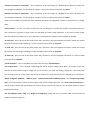
4. Open the file that you have just saved in a text editor. Make a note of the value of “multiplier” written in the pretext
then delete any text before (up to and including Begin: Data Text) and after (starting from # End: Data Text) the main
numerical data. This is shown in blue in the example.
5. Save this edited text file in the same directory as your MALTS software.
6. Start the executable (.exe file under Windows) to reach the user interface. The headings correspond to the following:
“Name of data file” – this is the name of the text file that you have just saved from the mmDisp
“Number of meshes in X direction” – this corresponds to the total length in x divided by the mesh size used in the
micromagnetic simulation. This should be an integer. It is also recorded in the text file as xnodes.
“Number of meshes in Y direction” - this corresponds to the total length in y divided by the mesh size used in the
micromagnetic simulation. This should be an integer. It is also recorded in the text file as ynodes.
“Number of meshes in Z direction” - this corresponds to the total length in z divided by the mesh size used in the
micromagnetic simulation. This should be an integer. It is also recorded in the text file as znodes.
If the incorrect number of meshes has been inputted, the boxes are highlighted in yellow to alert the user to change
them.
“Size of matrix” – the user can select any value for this, providing that it exceeds the number of meshes in both the x
and y directions. In general, a larger matrix size will allow for better image simulation. If you select a value smaller
than the number of meshes in the x and y directions, the box will turn yellow until the problem is rectified.
“X mesh size”- this is the size of the mesh used in the x direction in the micromagnetic simulation. Ideally this should
be small for optimal image simulating. It is also recorded in the text file as xstepsize.
“Y mesh size”- this is the size of the mesh used in the y direction in the micromagnetic simulation. Ideally this should
be small for optimal image simulating. It is also recorded in the text file as ystepsize.
“Z mesh size”- this is the size of the mesh used in the y direction in the micromagnetic simulation. It is also recorded
in the text file as zstepsize.
“Value multiplier” – this is recorded at the start of the text file as valuemultiplier.
“File output name” – this is what the LTEM image file will be saved as. MALTS saves both a screenshot of the user
interface and the Lorentz image as image files into its directory. To avoid overwriting, change this name every time
you run MALTS. Do not use the same name as that of the data file, since this will cause the data file to be overwritten.
“Beam divergence (radians)”, “defocus (µm)”, “spherical aberration coefficient (mm)” and “accelerating voltage
(kV)” are all experimental values corresponding to the specific LTEM experiment. The “mean inner potential (V)” is
specific to the material and typical values are cited on the user interface for ease of use. The default values are typical
experimental values.
“Tilt axis (degrees from x axis)” and “Angle of tilt (degrees)” enable the user to simulate LTEM contrast when the
sample is tilted (see Figure 2).
Figure 1: geometry for tilting the sample
The grey scale adjusters alter the colour limits to specified minimum and maximum values. Values less than cmin map
to cmin and values greater than cmax map to cmax. Those values between cmin and cmax are mapped linearly in grey
scale.
7. The “Lorentz TEM image” button on the right hand side simulates a Lorentz TEM image. White contrast means more
intensity reaching the screen, black contrast, less intensity. The “Electric Component LTEM image” buttons enables
the computation of an LTEM image with only electric and no magnetic contrast. Equally, if a magnetic component
LTEM image is required, just set the mean inner potential to zero. The “Profile” button shows the outline of the
structure considered. If this looks wrong but there are no yellow warning boxes, this could mean that the number of
meshes in the x and y directions are the wrong way around.
Example
Figure 2: Example file from OOMMF [1] to show which parameters to enter into the MALTS GUI (red). Text to be
deleted at the start of the text file before computation is highlighted in blue.
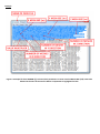
Figure 3: Text to be deleted at the end of the text file before computation is highlighted in blue.
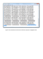
Figure 4: the Graphical User Interface for MALTS. Shown here is a simulation for the “example” text file shown in
Figures 2 and 3 of LTEM Fresnel mode contrast for a uniformly magnetised nanodisc of dimensions diameter 50nm,
thickness 20nm.
[1] Donahue, M.J. and Porter, D.G. OOMMF User's Guide, Version 1.0, Interagency Report NISTIR 6376, National
Institute of Standards and Technology, Gaithersburg, MD (Sept 1999), http://math.nist.gov/oommf
[2] Vansteenkiste, A. and Van de Wiele, B., MUMAX: A new high-performance micromagnetic simulation tool,
JOURNAL OF MAGNETISM AND MAGNETIC MATERIALS, {2011}, {323}, {2585-2591}
[3] Walton, S.K., Zeissler, K., Branford, W.R. and Felton, S., MALTS: A tool to simulate Lorentz Transmission Electron
Microscopy from micromagnetic simulations
Appendix: treatment of tilt in MALTS
Consider a LTEM simulation with a single mesh in the z direction. If the sample is tilted by “angle of tilt” degrees
about the x axis, the electron beam will no longer see the same sample dimensions and instead see its projection on
the xy plane. The sample will appear thicker in the z direction (z_thicker = z_init/cos(angle of tilt)) and compressed in
the y direction (y_compressed = y_init * cos(angle of tilt)). MALTS achieves this compression by resizing the matrix in
the y direction via a bicubic interpolation method.
Figure 3: compression in the y direction on rotation about the x axis by an angle of 30 degrees. The solid blue line is the untilted sample
profile and the dotted blue line is the tilted sample profile. The dashed black line represents the x axis, i.e. the axis of tilt.
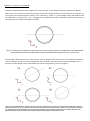
If the sample is tilted about an axis in the xy plane “tilt axis” degrees away from the x axis, the sample is rotated by
“tilt axis” degrees so that its tilt axis is aligned with the x’ direction. The compression is then performed in the y’
direction and the sample is then rotated back to its initial configuration by “tilt axis” degrees.
Figure 4: (a) the dashed black line indicates the axis of tilt and the solid blue line represents the untilted sample profile (b) the sample is
rotated such that the tilt axis is now in the x' direction (c) the sample is then compressed in the y' direction. The solid blue line represents
the untilted profile and the dotted blue line represents the tilted profile. (d) the sample is rotated back to its initial configuration. The
dotted blue line represents the profile of the sample having been tilted about the dashed black line axis.
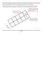
Now consider a simulation in which there are multiple meshes in the z direction. Exactly the same method as above
is used for each individual mesh. However, the meshes are not stacked directly on top of each other, with respect to
the electron beam after tilting, and are instead shifted with respect to each other by a distance
shift=zmesh*sin(tiltangle). The direction of the shift depends on the sign of the angle of rotation. This shift is
achieved in MALTS via a linear interpolation method in the y (or y’, if the tilt axis is not the x axis) direction.
Figure 5: when multiple meshes are tilted, they are no longer stacked directly on top of each other. Instead they are shifted with respect to
each other.