1
ANSYS ICEM
CFD/AI*Environment
10.0 User Manual
ANSYS ICEM CFD/AI*Environment
10.0 User Manual
Table of Contents
1. CAD Repair .......................................................................................................................................... 1–1
1.1. How are Close Holes and Remove Holes different? ......................................................................... 1–1
1.1.1. Close Holes .......................................................................................................................... 1–1
1.1.2. Remove Holes ...................................................................................................................... 1–2
1.2. How do Fill, Trim and Blend work in Stitch/Match Edges? ............................................................... 1–3
1.3. How does Match work in Stitch/Match Edges? ............................................................................... 1–5
2. Tetra .................................................................................................................................................... 2–1
2.1. Introduction ................................................................................................................................. 2–1
2.1.1. Tetra mesh generation ......................................................................................................... 2–1
2.1.2. Input to Tetra ....................................................................................................................... 2–1
2.2. Tetra Generation Steps ................................................................................................................. 2–2
2.2.1. Repair Geometry .................................................................................................................. 2–2
2.2.2. Geometry Details Required ................................................................................................... 2–3
2.2.3. Sizes on surfaces and curves ................................................................................................. 2–4
2.2.4. Meshing inside small angles or in small gaps between objects .............................................. 2–5
2.2.5. Desired Mesh Region ........................................................................................................... 2–5
2.2.6. Run Tetra - The Octree Approach .......................................................................................... 2–5
2.3. Important Features in Tetra ......................................................................................................... 2–12
2.3.1. Natural Size ........................................................................................................................ 2–12
2.3.2. Tetrahedral Mesh Smoother ............................................................................................... 2–12
2.3.3. Tetrahedral Mesh Coarsener ............................................................................................... 2–13
2.3.4. Triangular Surface Mesh Smoother ..................................................................................... 2–13
2.3.5. Triangular Surface Mesh Coarsener ..................................................................................... 2–13
2.3.6. Triangular Surface Editing Tools ......................................................................................... 2–13
2.3.7. Check Mesh ....................................................................................................................... 2–13
2.3.8. Quality metric .................................................................................................................... 2–18
2.3.9. Advanced options .............................................................................................................. 2–18
3. Hexa .................................................................................................................................................... 3–1
3.1. Introduction ................................................................................................................................. 3–1
3.2. Features of Hexa ........................................................................................................................... 3–1
3.3. Mesh Generation with Hexa .......................................................................................................... 3–2
3.4. The Hexa Database ....................................................................................................................... 3–2
3.5. Intelligent Geometry in Hexa ........................................................................................................ 3–2
3.6. Unstructured and Multi-block Structured Meshes .......................................................................... 3–3
3.6.1. Unstructured Mesh Output: .................................................................................................. 3–3
3.6.2. Multi-Block Structured Mesh Output: .................................................................................... 3–3
3.7. Blocking Strategy .......................................................................................................................... 3–3
3.7.1. Split ..................................................................................................................................... 3–4
3.7.2. Merge .................................................................................................................................. 3–4
3.8. Using the Automatic O-grid .......................................................................................................... 3–4
3.9. Most Important Features of Hexa .................................................................................................. 3–6
3.10. Automatic O-grid generation ...................................................................................................... 3–6
3.10.1. Important Features of an O-grid ......................................................................................... 3–7
3.11. Edge Meshing Parameters .......................................................................................................... 3–7
3.12. Smoothing Techniques ............................................................................................................... 3–7
3.13. Refinement and Coarsening ........................................................................................................ 3–8
3.13.1. Refinement ........................................................................................................................ 3–8
3.13.2. Coarsening ........................................................................................................................ 3–8
3.14. Replay Functionality ................................................................................................................... 3–8
3.14.1. Generating a Replay File ..................................................................................................... 3–8
ANSYS ICEM CFD/AI*Environment 10.0 User Manual . . © SAS IP, Inc.
ANSYS ICEM CFD/AI*Environment 10.0 User Manual
3.14.2. Advantage of the Replay Function ..................................................................................... 3–8
3.15. Periodicity .................................................................................................................................. 3–8
3.15.1. Applying the Periodic Relationship .................................................................................... 3–9
3.16. Mesh Quality .............................................................................................................................. 3–9
3.16.1. Determining the Location of Cells ....................................................................................... 3–9
3.16.2. Determinant ...................................................................................................................... 3–9
3.16.3. Angle ................................................................................................................................. 3–9
3.16.4. Volume .............................................................................................................................. 3–9
3.16.5. Warpage ............................................................................................................................ 3–9
4. Properties ............................................................................................................................................ 4–1
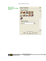
4.1. Create Material Property ............................................................................................................... 4–1
4.2. Save Material ................................................................................................................................ 4–1
4.3. Open Material ............................................................................................................................... 4–1
4.4. Define Table ................................................................................................................................. 4–1
4.5. Define Point Element .................................................................................................................... 4–1
4.6. Define Line Element ...................................................................................................................... 4–1
4.7. Define Shell Element .................................................................................................................... 4–1
4.8. Define Volume Element ................................................................................................................ 4–1
5. Constraints ......................................................................................................................................... 5–1
5.1. Displacement on Point .................................................................................................................. 5–1
5.2. Displacement on Curve ................................................................................................................. 5–1
5.3. Displacement on Area ................................................................................................................... 5–1
5.4. Displacement on Subset ............................................................................................................... 5–1
5.5. Define Contact ............................................................................................................................. 5–1
5.5.1. Automatic Detection ............................................................................................................ 5–1
5.5.2. Manual Definition ................................................................................................................ 5–1
5.6. Define Single Surface Contact ...................................................................................................... 5–1
5.7. Define Initial velocity .................................................................................................................... 5–1
5.8. Define Planar Rigid wall ................................................................................................................ 5–1
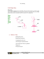
6. Loads ................................................................................................................................................... 6–1
6.1. Force on Point .............................................................................................................................. 6–6
6.2. Force on curve .............................................................................................................................. 6–6
6.3. Force on Surface ........................................................................................................................... 6–7
6.4. Force on Subset ............................................................................................................................ 6–7
6.5. Pressure on surfaces ..................................................................................................................... 6–7
6.6. Pressure on subset ........................................................................................................................ 6–7
6.7. Temperature on Points ................................................................................................................. 6–7
6.8. Temperature on curves ................................................................................................................. 6–7
6.9. Temperature on Surface ............................................................................................................... 6–7
6.10. Temperature on Body ................................................................................................................. 6–7
6.11. Temperature on Subset ............................................................................................................... 6–7
6.12. Set Gravity .................................................................................................................................. 6–7
7. Solver Options ..................................................................................................................................... 7–1
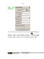
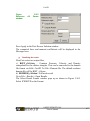
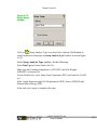
7.1. Setup Solver Parameters. .............................................................................................................. 7–1
7.2. Setup Analysis Type ...................................................................................................................... 7–1
7.3. Setup Sub-Case ............................................................................................................................ 7–1
7.4. Write/View Input file ..................................................................................................................... 7–1
7.5. Submit Solver Run ........................................................................................................................ 7–1
7.6. Post Process Results ...................................................................................................................... 7–1
7.7. FEA Solver Support ....................................................................................................................... 7–1
vi
ANSYS ICEM CFD/AI*Environment 10.0 User Manual . . © SAS IP, Inc.
ANSYS ICEM CFD/AI*Environment 10.0 User Manual
List of Figures
1.1. Close Hole .......................................................................................................................................... 1–2
1.2. After closing the hole .......................................................................................................................... 1–2
1.3. Before Remove Holes .......................................................................................................................... 1–3
1.4. After Remove Holes ............................................................................................................................ 1–3
1.5. Geometry with a gap .......................................................................................................................... 1–4
1.6. Result with Close Gap > Fill ................................................................................................................. 1–4
1.7. Result with Close Gap > Trim ............................................................................................................... 1–5
1.8. Result with Close Gap > Blend ............................................................................................................. 1–5
1.9. Geometry with mismatched edges ...................................................................................................... 1–6
1.10. Geometry after match edges ............................................................................................................. 1–7
2.1. Curves and Points representing the sharp edges and corners ............................................................... 2–3
2.2. Mesh with Curves and points .............................................................................................................. 2–4
2.3. Mesh without curves and points ......................................................................................................... 2–4
2.4. Geometry Input to Tetra ..................................................................................................................... 2–6
2.5. Full Tetra enclosing the geometry ....................................................................................................... 2–7
2.6. Full Tetra enclosing the geometry (In wire frame node) ....................................................................... 2–8
2.7. Cross-section of the Tetra to show how Tetra are fit in around geometry .............................................. 2–9
2.8. Mesh after it captures surfaces and separation of useful volume ........................................................ 2–10
2.9. Final Mesh before smoothing ............................................................................................................ 2–11
2.10. Final Mesh after smoothing ............................................................................................................. 2–12
2.11. Non-Manifold Vertices .................................................................................................................... 2–16
2.12. Quality Histogram ........................................................................................................................... 2–16
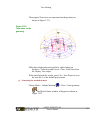
3.1. Initial block, block with O-Grid, O-Grid with include a face ................................................................... 3–5
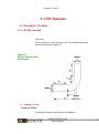
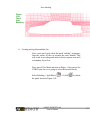
6.1. Elements on Curve .............................................................................................................................. 6–1
6.2. Force Distribution as per the FEA concepts .......................................................................................... 6–2
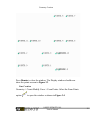
6.3. Quadratic Element Nodes position ...................................................................................................... 6–3
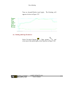
6.4. Load Distribution as per the FEA concepts ........................................................................................... 6–4
6.5. QUAD9 Element ................................................................................................................................. 6–5
ANSYS ICEM CFD/AI*Environment 10.0 User Manual . . © SAS IP, Inc.
vii
viii
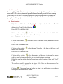
Chapter 1: CAD Repair
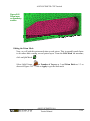
Before generating the Shell/Tetra mesh, the user should confirm that the geometry is free of any flaws that
would inhibit optimal mesh creation. If the user wishes to save the changes in the native CAD files, the following
checks should be performed in a direct CAD interface.
To create a mesh, Tetra requires that the model contains a closed volume. If there are any holes (gaps or missing
surfaces) in the geometry that are larger than the local tetras, Tetra will be unable to find a closed volume. Thus,
if the user notices any holes in the model prior to mesh generation, he or she should fix the surface data to
eliminate these holes.
The Build Topology operation will find holes and gaps in the geometry. It should give yellow curves where there
are large (in relation to a user-specified tolerance) gaps or missing surfaces.
During the Tetra process any leakage path (indicating a hole or gap in the model) will be indicated to the user.
The problem can be corrected on a mesh level, or the geometry in that vicinity can be repaired and the meshing
process repeated. For further information on the process of interactively closing holes, see the section Tetra >
Tetra Generation Steps > Useful Region of Mesh.
For more useful information on CAD Repair topics, please go to http://www-berkeley.ansys.com/faq/faq_topic_8.html.
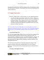
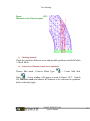
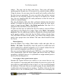
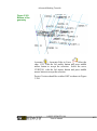
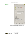
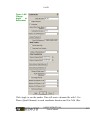
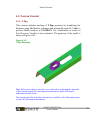
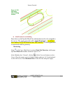
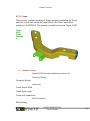
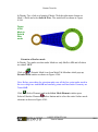
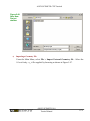
1.1. How are Close Holes and Remove Holes different?
1.1.1. Close Holes
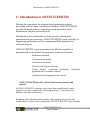
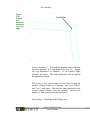
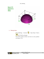
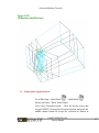
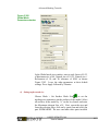
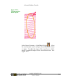
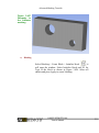
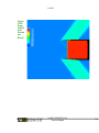
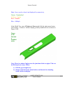
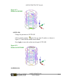
Use Close Holes if the hole is bounded by more than one surface. For example, look at Figure 1-1 below. The
yellow curves represent the boundary of the hole. From the figure it is clear that this hole is bounded by more
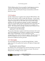
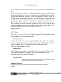
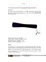
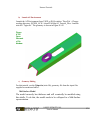
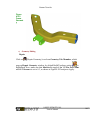
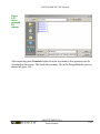
than one surface. Figure 1-2 shows the geometry after Close Holes is completed. A new surface is created to
close the hole.
ANSYS ICEM CFD/AI*Environment 10.0 User Manual . . © SAS IP, Inc.
Chapter 1: CAD Repair
Figure 1.1 Close Hole
Figure 1.2 After closing the hole
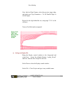
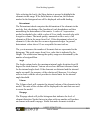
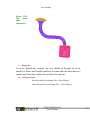
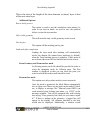
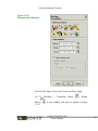
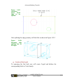
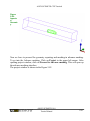
1.1.2. Remove Holes
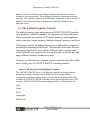
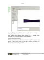
Use Remove Holes if the hole lies entirely within a single surface, such as a trimmed surface. For example, look
at Figure 1-3. The two yellow curve loops represent the boundaries of the holes, which lie entirely in one surface.
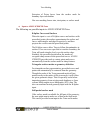
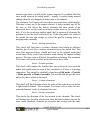
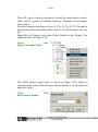
Figure 1-4 shows the geometry after Remove Holes is completed for one of the holes. The existing surface is
modified by removing the trim definition.
1–2
ANSYS ICEM CFD/AI*Environment 10.0 User Manual . . © SAS IP, Inc.
Section 1.2: How do Fill, Trim and Blend work in Stitch/Match Edges?
Figure 1.3 Before Remove Holes
Figure 1.4 After Remove Holes
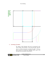
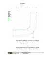
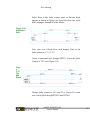
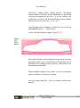
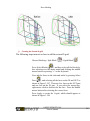
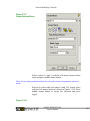
1.2. How do Fill, Trim and Blend work in Stitch/Match Edges?
Consider the case as shown in Figure 1.5: “Geometry with a gap”. The following figures explain how these work:
ANSYS ICEM CFD/AI*Environment 10.0 User Manual . . © SAS IP, Inc.
1–3
Chapter 1: CAD Repair
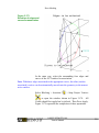
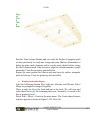
Figure 1.5 Geometry with a gap
Figure 1.6 Result with Close Gap > Fill
1–4
ANSYS ICEM CFD/AI*Environment 10.0 User Manual . . © SAS IP, Inc.
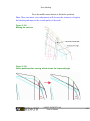
Section 1.3: How does Match work in Stitch/Match Edges?
Figure 1.7 Result with Close Gap > Trim
Figure 1.8 Result with Close Gap > Blend
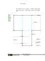
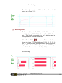
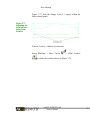
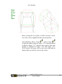
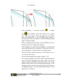
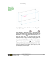
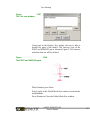
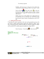
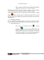
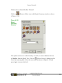
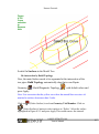
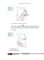
1.3. How does Match work in Stitch/Match Edges?
Match is generally used in those cases where curves lie very close to each other, specifically when the two ends
meet together. You should have the two sets of curves within some tolerance for this option to work. Refer to
the figures below to get an idea.
ANSYS ICEM CFD/AI*Environment 10.0 User Manual . . © SAS IP, Inc.
1–5
Chapter 1: CAD Repair
Figure 1.9 Geometry with mismatched edges
1–6
ANSYS ICEM CFD/AI*Environment 10.0 User Manual . . © SAS IP, Inc.
Section 1.3: How does Match work in Stitch/Match Edges?
Figure 1.10 Geometry after match edges
ANSYS ICEM CFD/AI*Environment 10.0 User Manual . . © SAS IP, Inc.
1–7
1–8
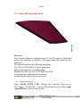
Chapter 2: Tetra
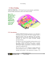
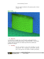
Automated to the point that the user has only to select the geometry to be meshed, Tetra generates tetrahedral
meshes directly from the CAD geometry or STL data, without requiring an initial triangular surface mesh.
2.1. Introduction
Tetra uses an Octree-based meshing algorithm to fill the volume with tetrahedral cells and to generate a surface
mesh on the object surfaces. The user can define prescribed curves and points to determine the positions of
edges and vertices in the mesh. For improved cell quality, Tetra incorporates a powerful smoothing algorithm,
as well as tools for local adaptive mesh refinement and coarsening.
For more useful information on Tetra, please go to http://www-berkeley.ansys.com/faq/faq_topic_2.html.
2.1.1. Tetra mesh generation
Suitable for complex geometries, Tetra offers several advantages, including:
•
Rapid model set-up
•
Mesh is independent of underlying surface topology
•
No surface mesh necessary
•
Generation of mesh directly from CAD or STL surfaces
•
Definition of cell size on CAD or STL surfaces
•
Control over cell size inside a volume
•
Nodes and edges of tetrahedra are matched to prescribed points and curves
•
Natural size automatically determines tetrahedra size for individual geometry features
•
Volume and surface mesh smoothing, merging nodes and swapping edges
•
Tetrahedral mesh can be merged into another tetra, hexa or hybrid mesh and then can be smoothed
•
Coarsening of individual material domains
•
Enforcement of mesh periodicity, both rotational and translational
•
Surface mesh editing and diagnostic tools
•
Local adaptive mesh refinement and coarsening
•
One consistent mesh for multiple materials
•
Fast algorithm: 1500 cells/second
•
Automatic detection of holes and easy way to repair the mesh
•
For more details, go to Run Tetra - The Octree Approach
.
2.1.2. Input to Tetra
The following are possible inputs to Tetra:
•
Sets of B-Spline curves and trimmed B-Spline surfaces with prescribed points
ANSYS ICEM CFD/AI*Environment 10.0 User Manual . . © SAS IP, Inc.
Chapter 2: Tetra
•
Triangular surface meshes as geometry definition
•
Full/partial surface meshes
B-Spline Curves and Surfaces
When the input is a set of B-Spline curves and surfaces with prescribed points, the mesher approximates the
surface and curves with triangles and edges respectively; and then projects the vertices onto the prescribed
points.
The B-Spline curves allow Tetra to follow discontinuities in surfaces. If no curves are specified at a surface
boundary, Tetra will mesh triangles freely over the surface edge. Similarly, prescribed points allow the mesher
to recognize sharp corners in the geometry. ANSYS ICEM CFD provides tools (Build Topology) to extract points
and curves to define sharp features in the surface model.
Triangular surface meshes as geometry definition
Prescribed curves and points can also be extracted from triangulated surface geometry. This could be stereolithography (STL) data or a surface mesh converted to faceted geometry. Though the nodes of the Tetra -generated
mesh will not exactly match the nodes of the given triangulated geometry, they will follow the overall shape. A
geometry for meshing can contain both faceted and B-Spline geometry.
Full/partial surface mesh
Existing surface mesh for all or part of the geometry can be specified as input to Tetra . The final mesh will then
be consistent with and connected to the existing mesh nodes.
2.2. Tetra Generation Steps
The steps involved in generating a Tetra mesh are:
•
Geometry Repair/Clean up
•
Geometry details required
•
Sizes on Surfaces/Curves
•
Meshing inside small angles or in small gaps between objects
•
Desired Mesh Region
•
Run Tetra - The Octree Approach
•
Check the mesh for errors
•
Edit mesh to correct any errors
•
Smooth the mesh to improve quality
The mesh is then ready to apply loads, boundary conditions, etc., and for writing to the desired solver.
2.2.1. Repair Geometry
Refer to the CAD Repair section.
2–2
ANSYS ICEM CFD/AI*Environment 10.0 User Manual . . © SAS IP, Inc.
Section 2.2: Tetra Generation Steps
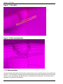
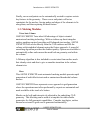
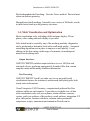
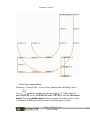
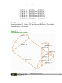
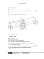
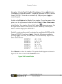
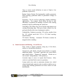
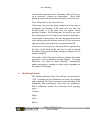
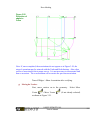
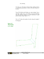
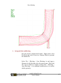
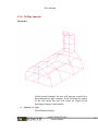
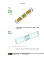
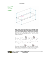
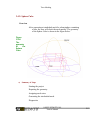
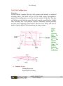
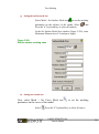
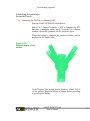
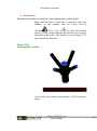
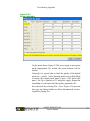
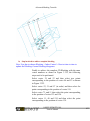
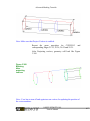
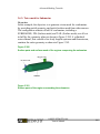
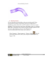
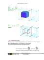
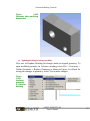
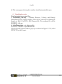
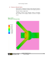
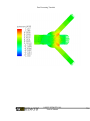
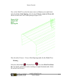
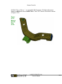
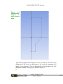
2.2.2. Geometry Details Required
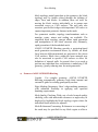
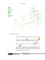
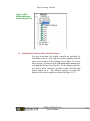
In addition to a closed set of surfaces, Tetra requires curves and points where hard features (hard angles, corners)
are to be captured in the mesh. The first figure below shows a set of curves and points representing hard features
of the geometry, where the second and third figure show the resultant mesh with and without the curves and
points preserved.
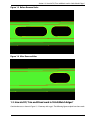
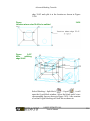
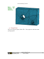
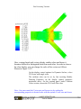
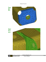
Figure 2 shows the resultant surface mesh if the curves and points are preserved in the geometry. Mesh nodes
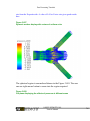
are forced to lie along the curves and points to capture the hard features of the geometry. Figure 3 shows the
resultant surface mesh if the curves and points are deleted from the geometry. The hard features of the geometry
are not preserved, but rather are neglected or chamfered. The boundary mesh nodes lie on the surfaces, but
they will only lie on the edges of the surfaces if curves and points are present. Removal of curves and points can
be used as a geometry defeaturing tool.
Figure 2.1 Curves and Points representing the sharp edges and corners
ANSYS ICEM CFD/AI*Environment 10.0 User Manual . . © SAS IP, Inc.
2–3
Chapter 2: Tetra
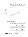
Figure 2.2 Mesh with Curves and points
Figure 2.3 Mesh without curves and points
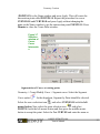
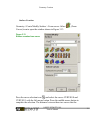
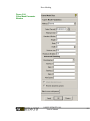
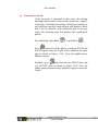
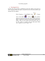
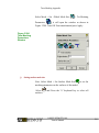
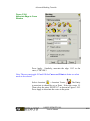
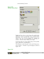
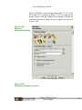
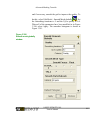
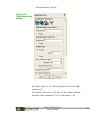
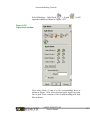
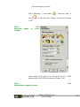
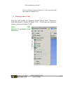
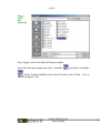
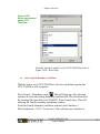
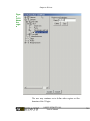
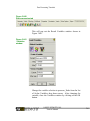
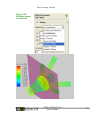
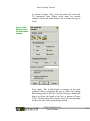
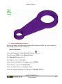
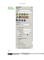
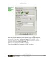
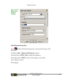
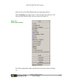
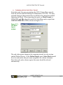
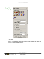
2.2.3. Sizes on surfaces and curves
To produce the optimal mesh, it is essential that all surfaces and curves have the proper tetra sizes assigned to
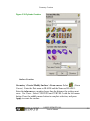
them. For a visual representation of the mesh size, select Geometry > Surfaces > Surface Tetra sizes from the
Display Tree. The same can be done with Curves. Tetra icons will appear, representing the cell size of the mesh
to be created on these entities. With the mouse, the user may rotate the model and visually confirm that the
tetra sizes are appropriate. If a curve or surface does not have an icon plotted on it, the icon may be too large or
too small to see. In this case, the user should modify the mesh parameters so that the icons are visible in a normal
display.
2–4
ANSYS ICEM CFD/AI*Environment 10.0 User Manual . . © SAS IP, Inc.
Section 2.2: Tetra Generation Steps
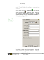
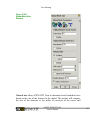
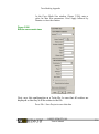
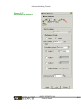
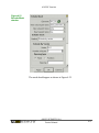
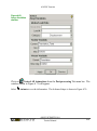
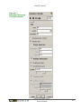
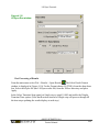
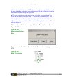
The user should also make sure that a reference cell size has been defined. To modify the mesh size for all entities,
adjust the Scale Factor, which is found in Set Global Mesh Size window from Mesh Tabbed menubar. Note
that if 0 is assigned as the Scale Factor, Tetra will not run.
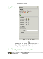
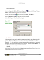
2.2.4. Meshing inside small angles or in small gaps between objects
Examine the regions between two surfaces or curves that are very close together or that meet at a small angle.
(This would also apply if the region outside the geometry has small angles.) If the local tetra sizes are not small
enough so that at least 1 or 2 elements would fit through the thickness, the user should define Thin cuts. This is
in the Tet Meshing Parameters section of the Global Mesh Size window. To define a thin cut, the two surfaces
have to be in different Parts. If the surfaces meet, the curve at the intersection of the surfaces will need to be in
a third, different Part.
If the tetra sizes are larger or approximately the same size as the gap between the surfaces or curves, the surface
mesh could have a tendency to jump the gap, thus creating non-manifold vertices. These non-manifold vertices
would be created during the Tetra process. Tetra automatically attempts to close all holes in a model. Since the
gap may be confused as a hole, the user should either define a thin cut, in order to establish that the gap is not
a hole; or make the mesh size small enough so that it won't close the gap when the Tetra process is performed.
A hole is usually considered a space that is greater than 2 or 3 cells in thickness.
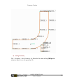
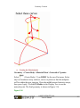
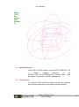
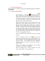
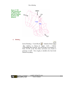
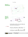
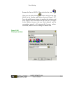
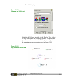
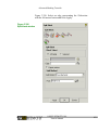
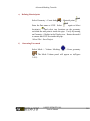
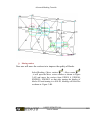
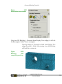
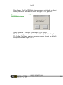
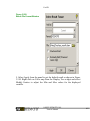
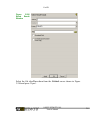
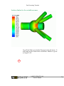
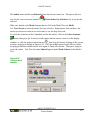
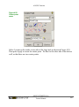
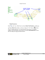
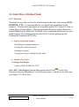
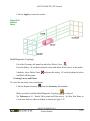
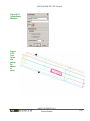
2.2.5. Desired Mesh Region
During the process of finding the bounding surfaces to close the volume mesh, the mesher will determine if
there are holes in the model. If there are, the messages window will display a message like "Material point ORFN
can reach material point LIVE." You will be prompted with a dialog box saying, "Your geometry has a hole, do
you want to repair it?" A jagged line will display the leakage path from the ORFN part to the LIVE part. The cells
surrounding the hole will also be displayed. To repair the hole, select the single edges bounding it - and the
mesher will loft a surface mesh to close the hole. Further holes would be flagged and repaired in the same
manner. If there are many problem areas, it may be better to repair the geometry or adjust the meshing parameters.
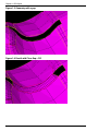
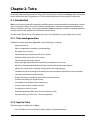
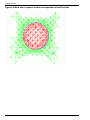
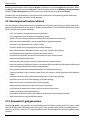
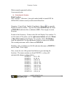
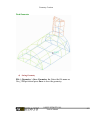
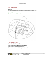
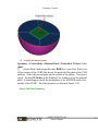
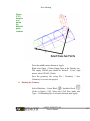
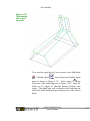
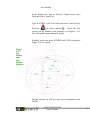
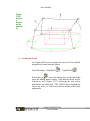
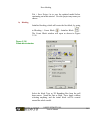
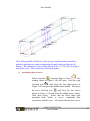
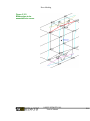
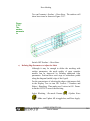
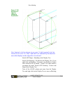
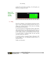
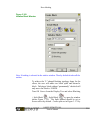
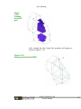
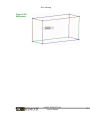
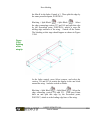
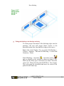
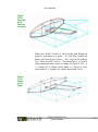
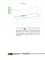
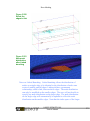
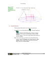
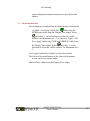
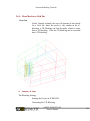
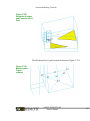
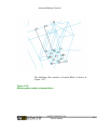
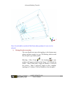
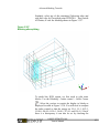
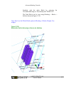
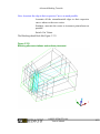
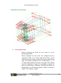
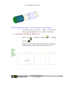
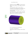
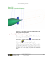
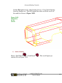
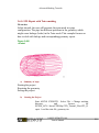
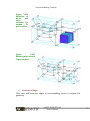
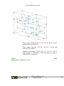
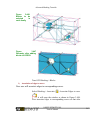
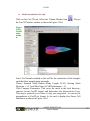
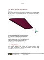
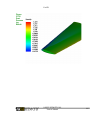
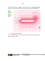
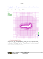
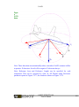
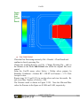
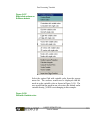
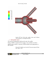
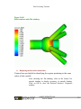
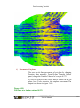
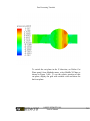
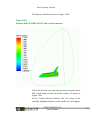
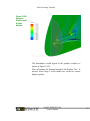
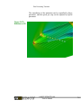
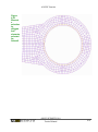
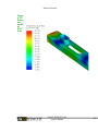
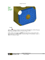
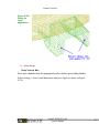
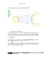
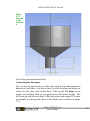
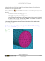
2.2.6. Run Tetra - The Octree Approach
Tetra's mesh generation is based on the following spatial subdivision algorithm: This algorithm ensures refinement
of the mesh where necessary, but maintains larger cells where possible, allowing for faster computation. Once
the "root" tetrahedron, which encloses the entire geometry, has been initialized, Tetra subdivides the root tetrahedron until all cell size requirements are met.
ANSYS ICEM CFD/AI*Environment 10.0 User Manual . . © SAS IP, Inc.
2–5
Chapter 2: Tetra
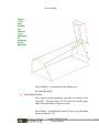
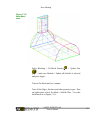
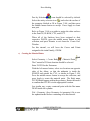
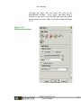
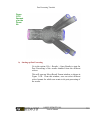
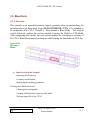
Figure 2.4 Geometry Input to Tetra
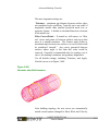
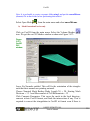
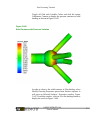
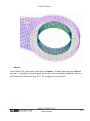
At this point, the Tetra mesher balances the mesh so that cells sharing an edge or face do not differ in size by
more than a factor of 2.
2–6
ANSYS ICEM CFD/AI*Environment 10.0 User Manual . . © SAS IP, Inc.
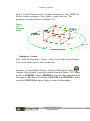
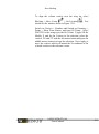
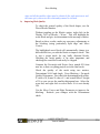
Section 2.2: Tetra Generation Steps
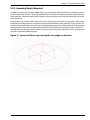
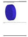
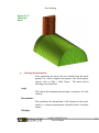
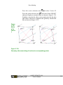
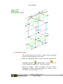
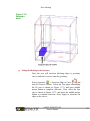
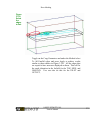
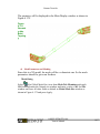
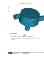
Figure 2.5 Full Tetra enclosing the geometry
ANSYS ICEM CFD/AI*Environment 10.0 User Manual . . © SAS IP, Inc.
2–7
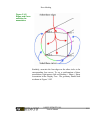
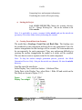
Chapter 2: Tetra
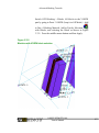
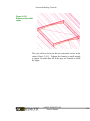
Figure 2.6 Full Tetra enclosing the geometry (In wire frame node)
2–8
ANSYS ICEM CFD/AI*Environment 10.0 User Manual . . © SAS IP, Inc.
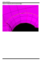
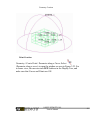
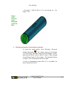
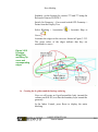
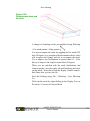
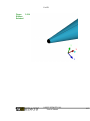
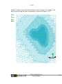
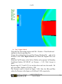
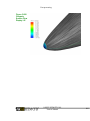
Section 2.2: Tetra Generation Steps
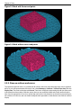
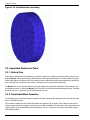
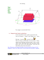
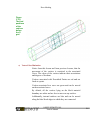
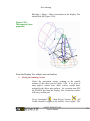
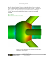
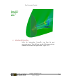
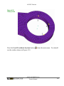
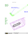
Figure 2.7 Cross-section of the Tetra to show how Tetra are fit in around geometry
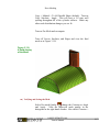
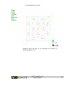
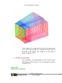
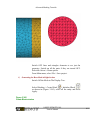
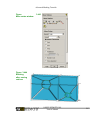
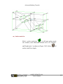
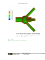
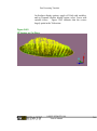
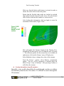
After this is done, Tetra makes the mesh conformal - that is, it guarantees that each pair of adjacent cells will
share an entire face. The mesh does not yet match the given geometry, so the mesher next rounds the nodes of
the mesh to the prescribed points, prescribed curves or model surfaces. Tetra then "cuts away" all of the mesh,
which cannot be reached by a user-defined material point without intersection of a surface.
ANSYS ICEM CFD/AI*Environment 10.0 User Manual . . © SAS IP, Inc.
2–9
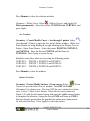
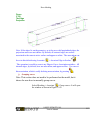
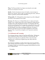
Chapter 2: Tetra
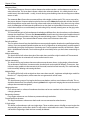
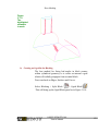
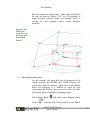
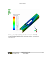
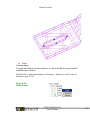
Figure 2.8 Mesh after it captures surfaces and separation of useful volume
2–10
ANSYS ICEM CFD/AI*Environment 10.0 User Manual . . © SAS IP, Inc.
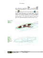
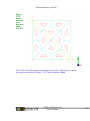
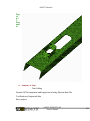
Section 2.2: Tetra Generation Steps
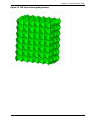
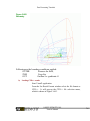
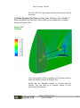
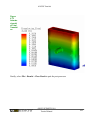
Figure 2.9 Final Mesh before smoothing
Finally, the mesh is smoothed by moving nodes, merging nodes, swapping edges and in some cases, deleting
bad cells.
ANSYS ICEM CFD/AI*Environment 10.0 User Manual . . © SAS IP, Inc.
2–11
Chapter 2: Tetra
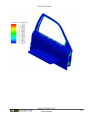
Figure 2.10 Final Mesh after smoothing
2.3. Important Features in Tetra
2.3.1. Natural Size
If the maximum tetrahedral size defined on a surface is larger than needed to resolve the feature, the user can
employ Natural size to automatically subdivide the mesh to capture the feature. The value specified is proportional to the global scale factor, and is the smallest size to be achieved through automatic element subdivision.
Even with large sizes specified on the surfaces, the features can be captured automatically.
The Natural size is the minimum element size to be achieved via automatic subdivision. If the maximum size
on a geometry entity is smaller than Natural size, Tetra will still subdivide to meet that requested size. The effect
of the natural size is a geometry- based adaptation of the mesh.
2.3.2. Tetrahedral Mesh Smoother
In smoothing the mesh, the tetrahedral smoother calculates individual cell quality based on the selection from
the list of available criteria.
The smoother modifies the cells with quality below the specified "Up to quality" value. Nodes can be moved
and/or merged, edges are swapped, and in some cases cells are deleted. This operation is then repeated on the
improved grid, up to the specified number of iterations. The user can choose to smooth some element types
while freezing others.
2–12
ANSYS ICEM CFD/AI*Environment 10.0 User Manual . . © SAS IP, Inc.
Section 2.3: Important Features in Tetra
2.3.3. Tetrahedral Mesh Coarsener
During the coarsening process the user can exclude surface or material domains by selecting those Parts in the
Parts to freeze panel. If the Maintain surface sizes option is enabled during coarsening, the resulting mesh
satisfies the specified mesh size criteria on the geometric entities.
2.3.4. Triangular Surface Mesh Smoother
The triangular surface mesh inherent in the Tetra mesh generation process can also be used independently of
the volume mesh. The triangular smoother marks all cells that are initially below the quality criterion and then
runs the specified number of smoothing steps on the cells. Nodes are moved on the actual CAD surfaces to improve
the quality of the cells.
2.3.5. Triangular Surface Mesh Coarsener
In the interest of minimizing grid points, the coarsener reduces the number of triangles in a mesh by merging
triangles. This operation is based on the maximum deviation of the resultant triangle center from the surface,
the aspect ratio of the merged triangle and the maximum size of the merged triangle.
2.3.6. Triangular Surface Editing Tools
For the interactive editing of surface meshes, Tetra offers a mesh editor in which nodes can be moved on the
underlying CAD surfaces, merged or even deleted. Individual triangles of the mesh can be subdivided or tagged
with different names. The user can perform the quality checks, as well as local smoothing.
Diagnostic tools for surface meshes allow the user to fill holes easily in the surface mesh. Also there are tools for
the detection of overlapping triangles and non-manifold vertices, as well as detection of single/multiple edge
and duplicate cells.
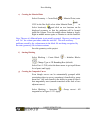
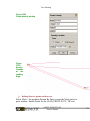
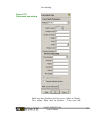
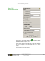
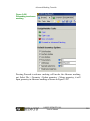
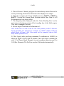
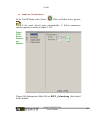
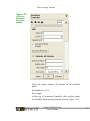
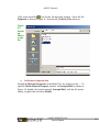
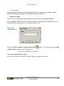
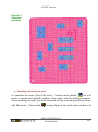
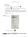
2.3.7. Check Mesh
Check the validity of the mesh using Edit Mesh > Check Mesh.
You can opt to Create subsets for each of the problems so that they can be fixed later or can opt to Check/fix
each one of them. Using subset manipulation and mesh editing techniques, diagnose the problem and resolve
it through merging nodes, splitting edges, swapping edges, delete/create cells, etc.
For ease of use when working with subsets, it is usually helpful to add elements to the subset in order to see
what is happening around the problem elements. This is done via a right-click on the Subset name in the Display
tree and then adding layers of elements to the subset. It can also be useful to display the element nodes and/or
display the elements slightly smaller than actual size. Both of these options can be accessed via a right-click on
"Mesh" from the Tree widget.
Keep in mind that after mesh editing, the diagnostics should be re-checked to verify that no mistakes were made.
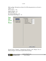
There are several Errors as well as Possible problems checks. The descriptions of these are as follows:
Duplicate elements
This check locates cells that share all of their nodes with other cells of the same type. These cells should be deleted.
Note — Note that deletion during the automatic fix will remove one of the two duplicate elements, thus
eliminating this error without creating a hole in the geometry.
ANSYS ICEM CFD/AI*Environment 10.0 User Manual . . © SAS IP, Inc.
2–13
Chapter 2: Tetra
Uncovered faces
This check will locate any face on a volume element that neither touches a surface element nor touches another volume face. This error often indicates a hole in the volumetric domain. It is unlikely that this error
would occur in the initial model -- usually, it results during manual editing when the user happens to delete
tetra or tri cells.
The automatic Fix will cover these uncovered faces with triangles (surface mesh). This may or may not be
the proper solution. A better method may be for the user to first Select the flawed cells and then decide if
the uncovered faces are the result of missing surface mesh or the result of a hole. If it is due to missing surface
mesh, the Fix option will eliminate the problem (re-run the check and select Fix). If the error points out a
hole in the model, the user could attempt to correct the grid by manually creating tetras or merging nodes.
Missing internal faces
This check will find pairs of volume elements that belong to different Parts, but do not have a surface element
between the shared faces. This error, like Uncovered faces, should not occur in the original model and would
most likely result from mistakes made during the manual editing process. The tetra cutter will detect this
problem as a leakage. The automatic Fix will create surface mesh in between these cells.
Periodic problems
The user selects the two Parts that should be one-to-one periodic matches based on the specified periodicity
settings. Errors are reported if periodic matches are missing. Slight offsets in node positions are often repaired
automatically during the check process. Remaining errors can be repaired manually via Edit Mesh > Repair
Mesh > Make/Remove Periodic. You should not get this error ideally unless you have done some editing on
the mesh.
Volume orientations
This check will find cells where the order of the nodes does not define a right-handed cell. The automatic
Fix will re-order the mis-oriented cells' nodes to eliminate this error.
Surface orientations
This check will flag any location where more than one tet element share a single triangle surface element.
The tet elements would have 3 common nodes, but the fourth node would be different. These errors, that
indicate a major problem in the connectivity in the model, need to be fixed manually. This would normally
involve manually deleting and creating elements.
Multiple Edges
This check will find cells with an edge that shares more than two cells. Legitimate multiple edges would be
found at a "T"-shaped junction, where more than two geometrical surfaces meet.
Triangle boxes
This check locates groups of 4 triangles that form a tetrahedron, with no actual volume cell inside. This undesirable characteristic is best fixed by choosing Select for this region and merging the two nodes that would
collapse the unwanted triangle box.
Hanging elements
For a volume mesh, a surface or line element that does not have an attached volume element is flagged as
a hanging element.
Penetrating elements
Flags regions where two sets of elements penetrate through each other.
Disconnected bar elements
This flags line elements where one or both nodes are not connected to other elements.
2-Single edges
This locates surface elements with two single edges. These are either corners of baffles or are triangles that
are protruding from a surface like a shark's fin and are thus undesirable in the mesh. These elements are a
subset of the single edges check and can normally be deleted.
2–14
ANSYS ICEM CFD/AI*Environment 10.0 User Manual . . © SAS IP, Inc.
Section 2.3: Important Features in Tetra
Single-Multiple edges
This check locates elements that have both single and multiple edges.
Stand-alone surface mesh
This check locates surface elements that do not share a face with a volume element. This could be an area
with an extra surface element to be deleted or a missing volume element to be created.
Single edges
This check will locate surface cells that have an edge that isn't shared with any other surface cell. This would
represent a hanging edge and the cell would be considered an internal baffle. These may or may not be legitimate. Legitimate single edges would occur where the geometry has a zero thickness baffle with a free
or hanging edge or in a 2D model at the perimeter of the domain.
If the single edges form a closed loop -- a hole in the surface mesh -- the user can select Fix when prompted
from the appearing menu. A new set of triangles will then be created to eliminate the hole.
Delaunay-violation
This check finds cells which violate the Delaunay rule, which states that a circumscribed circle around a surface
triangle should not enclose any other nodes. These can often be removed by swapping edges of these triangles.
Overlapping elements
This flags surface elements that occupy part of the same surface area, but don't share the same nodes (so
are not duplicates).
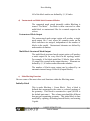
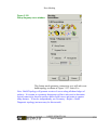
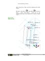
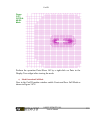
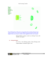
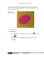
Non-manifold vertices
This check will find vertices who adjacent cells' outer edges don't form a closed loop. Finding this problem
usually indicates the existence of cells that jump from one surface to another, forming a "tent"-like structure,
as shown in the figure below.
ANSYS ICEM CFD/AI*Environment 10.0 User Manual . . © SAS IP, Inc.
2–15
Chapter 2: Tetra
Figure 2.11 Non-Manifold Vertices
Un-connected vertices
This check finds vertices that are not connected to any cells. These can generally be deleted.
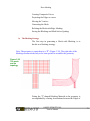
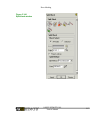
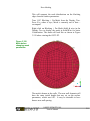
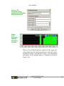
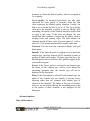
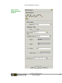
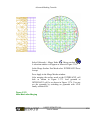
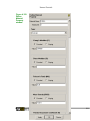
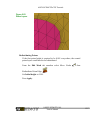
Smoothing
After eliminating errors/possible problems from a tetra grid, the user needs to smooth the grid to improve
the quality.
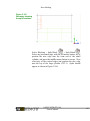
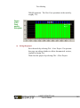
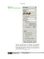
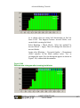
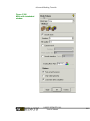
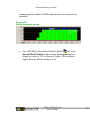
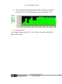
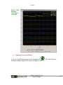
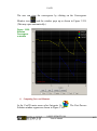
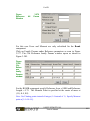
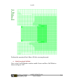
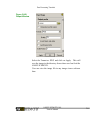
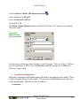
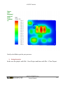
Figure 2.12 Quality Histogram
2–16
ANSYS ICEM CFD/AI*Environment 10.0 User Manual . . © SAS IP, Inc.
Section 2.3: Important Features in Tetra
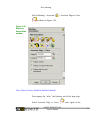
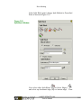
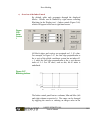
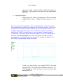
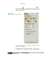
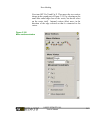
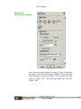
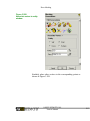
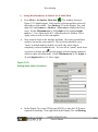
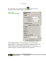
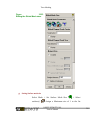
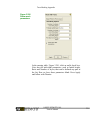
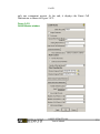
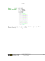
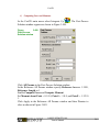
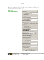
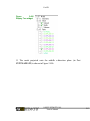
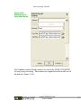
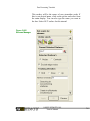
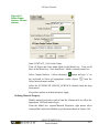
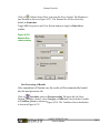
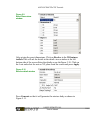
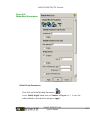
Histogram: The tetrahedral Quality will be displayed within this histogram, where 0 represents the worst aspect
ratio and 1 represents the best aspect ratio. The user may modify the display of the histogram by adjusting the
values of Min, Max, Height and Bars.
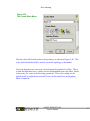
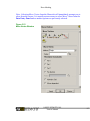
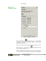
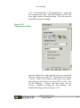
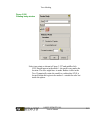
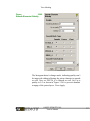
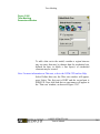
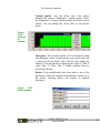
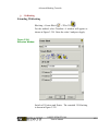
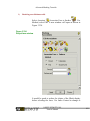
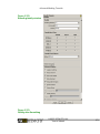
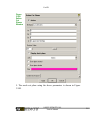
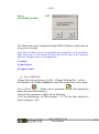
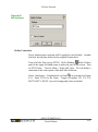
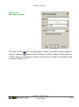
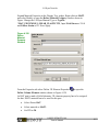
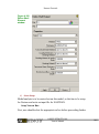
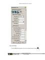
Replot: If any modification is to be done for displaying the histogram then select Replot which pops ups the
Replot window shown above. User can change the following parameters in this window, pressing Accept will
replot the histogram to the newly set values.
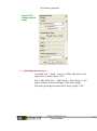
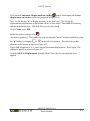
Min X Value: This minimum value, which is located on the left-most side of the histogram's x-axis, represents
the worst quality cells.
Max X Value: This maximum value, which is located on the right-most side of the histogram's x-axis, represents
the highest quality that cells can achieve.
Max Y height: The user can adjust the number of cells that will be represented on the histogram's y-axis. Usually
a value of 20 is sufficient. If there are too many cells displayed, it is difficult to discern the effects of smoothing.
Num bars: This represents the number of subdivisions within the range between the Min and the Max. The
default Bars have widths of 0.05. Increasing the amount of displayed bars, however, will decrease this width.
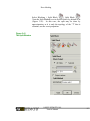
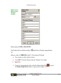
•
Reset: Selecting this option will return all of the values back to the original parameters that were present
when the Smooth cells window was first invoked.
•
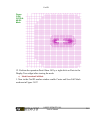
Show: The user may press the left mouse button on any of the bars in the histogram and the color will
change from green to pink. Toggling ON Show will display the cells that fall within the selected range on
the model in the main viewing window.
•
Solid: This toggle option will display the cells as solid tetras, rather than as the default grid representation.
The user will have to select Show, as well, to activate this option.
•
Subset: If the user has highlighted bars from the histogram and toggled ON Show, the cells displayed in
white color are also placed into a Subset. The visibility of this subset is controlled by Subset from the
Display Tree. Add select: This option allows the user to add cells to an already established subset.
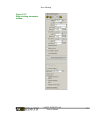
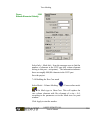
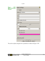
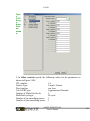
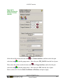
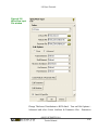
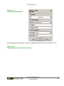
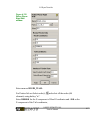
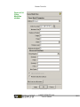
Smoothing Elements window:
Smoothing iterations: This value is the number of times the smoothing process will be performed.
Models with a more complicated geometry will require a greater number of iterations to obtain the
desired quality, which is assigned in Up to quality.
Up to quality: As mentioned previously, the Min value represents the worst quality of cells, while the Max value
represents the highest quality cells. Usually, the Min is set at 0.0 and the Max is set at 1.0. The Up to quality
value gives the smoother a quality to aim for. Ideally, after smoothing, the quality of the cells should be higher
ANSYS ICEM CFD/AI*Environment 10.0 User Manual . . © SAS IP, Inc.
2–17
Chapter 2: Tetra
than or equal to this value. If this does not happen, the user should find other methods of improving the quality,
such as merging nodes and splitting edges. For most models, the cells should all have ratios of greater than 0.3,
while a ratio of 0.15 for complicated models is usually sufficient.
•
Freeze: If the Freeze option is selected for a cell type, the nodes of this cell type will be fixed during the
smoothing operation; thus, the cell type will not be displayed in the histogram.
•
Float: If the Float option is selected for a cell type, the nodes of the cell type are capable of moving freely,
allowing nodes that are common with another type of cell to be smoothed. The quality of elements set
to Float is not tracked during the smoothing process and so the quality is not displayed in the histogram.
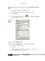
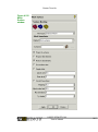
2.3.8. Quality metric
Changing this option allows the user to modify what the histogram displays.
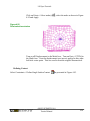
Quality: This histogram displays the overall quality of the mesh. The x-axis measures the quality, with 0 representing poor quality and 1 representing high quality. The y-axis measures the number of cells that belong within
each quality sub-range. Aspect ratio: For HEXA_8 (hexahedral) and QUAD_4 (quadrilateral) cells, the Aspect
ratio is defined as the ratio of the distances between diagonally opposite vertices (shorter diagonal/longer diagonal). For TETRA_4 (tetrahedral) cells, MED calculates the ratio between the radii of an inscribed sphere to a
circumscribed sphere for each cell. For TRI_3 (triangular) cells, this operation is done using circles. An Aspect
ratio of 1 is a perfect cell and an Aspect ratio of 0 indicates that the cell has zero volume. Determinant: This
histogram is based on the determinant of the Jacobian matrix. The Jacobian value is based on the difference
between the internal angles of the opposing edges within the cell.Min angle: The Min angle option yields a
histogram based upon the minimum internal angle of the cell edges.Max warp: This histogram is based on the
warpage of the quad faces of the prism. This is based on the worst angle between two triangles that make up
the quad face. Skew: This histogram is based upon calculations of the maximum skewness of a hexahedral or
quadrilateral cell. The skewness is defined differently for volume and surface cells. For a volume cell, it is obtained
by taking all pairs of adjacent faces and computing the normals. The maximum value thus obtained, is normalized
so that 0 corresponds to perpendicular faces and 1 corresponds to parallel faces. Custom quality: One can define
one's own quality definition by going to Diagnostics > Quality metrics. Select the Diagnostic: as Custom
quality and go for Define custom quality. One can change the values there to suit his/her needs.
2.3.9. Advanced options
Prism warpage Ratio
Prisms are smoothed based on a balance between prism warpage and prism aspect ratio. Numbers from
0.01 to 0.50 favor improving the prism aspect ratio, and from 0.50 to 0.99 favor improving prism warpage.
A value of 0.5 favors neither. The farther the value is from 0.5, the greater the effect.
Stay on geometry
This is the default where normally, when a grid is smoothed, the nodes are restricted to the geometry -surface, curves and points -- and can only be moved along the geometrical entities to obtain a better mesh.
Violate geometry Tolerance
Selecting this option allows the smoothing operation to yield a higher quality mesh by violating the constraints
of the geometry. The nodes can be moved off of the geometry to obtain better mesh quality, as long as the
movement remains within the absolute distance specified by the user.
Violate geometry Relative Tolerance
This option works in the similar fashion as above except that the distance is relative here.
Allow refinement
If the quality of the mesh cannot be improved through normal algebraic smoothing, Allow refinement will
allow the smoother to automatically subdivide tetras to obtain further improvement. After smoothing with
2–18
ANSYS ICEM CFD/AI*Environment 10.0 User Manual . . © SAS IP, Inc.
Section 2.3: Important Features in Tetra
Allow refinement selected, it may be necessary to Smooth further with the option turned off. The goal of
this option is to reduce the number of cells that are attached to one vertex by refinement in problem regions.
Laplace smoothing
This option will solve the Laplace equation, which will generally yield a more uniformly spaced mesh.
Note — This can sometimes lead to a lower determinant quality of the prisms. Also, this option works
only for the triangular surface mesh.
Allow node merging
This option will collapse and remove the worst tetra and prism elements when smoothing in order to obtain
a higher quality mesh. This default option is often very useful in improving the grid quality.
Not just worst 1%
This option will smooth all of the geometry's cells to the assigned quality -- specified under Up to quality - not just focus on the worst 1% of the mesh. Typically, when a mesh is smoothed, the smoother concentrates
on improving the worst regions; this option will allow the smoother to continue smoothing beyond the
worst regions until the desired quality is obtained.
Surface fitting
This option will smooth mesh, keeping the nodes and the new mesh restricted along the surface of the
geometry. Only Hexa models will utilize this option.
Ignore pre points
Selecting this option will allow the smoother to attempt to improve the mesh quality without being bound
by the initial points of the geometry. This option is similar to the Violate geometry option, but works only
for points located on the geometry. This option is available only when the user has hexahedral cells in the
model. Usually, the best way to improve the quality of grids that cannot be smoothed above a certain level
is to concentrate on the surface mesh near the bad cells and edit this surface mesh to improve the quality.
ANSYS ICEM CFD/AI*Environment 10.0 User Manual . . © SAS IP, Inc.
2–19
2–20
Chapter 3: Hexa
Hexa is a 3-D object-based, semi-automatic, multi- block structured and unstructured, surface and volume
mesher.
3.1. Introduction
Hexa represents a new approach to hexahedral mesh generation. The block topology model is generated directly
on the underlying CAD geometry. Within an easy-to-use interface, those operations most often performed by
experts are readily accessible through automated features.
Recognized as the fastest hexahedral mesh generation tool in the market, ICEM CFD 4.CFX allows users to
generate high-quality meshes for aerospace, automotive, computer and chemical industry applications in a
fraction of the time required for traditional tools.
The user has access to two types of entities during the mesh generation process in Hexa: block topology and
geometry. After interactively creating a 3-D block topology model equivalent to the geometry, the block topology
may be further refined through the splitting of edges, faces and blocks. In addition, there are tools for moving
the block vertices -- individually or in groups -- onto associated curves or CAD surfaces. The user may also associate specific block edges with important CAD curves to capture important geometric features in the mesh.
Moreover, for models where the user can take advantage of symmetry conditions, topology transformations
such as translate, rotate, mirror and scaling are available. The simplified block topology concept allows rapid
generation and manipulation of the block structure and, ultimately, rapid generation of the hexahedral meshes.
Hexa provides a projection-based mesh generation environment where, by default, all block faces between
different materials are projected to the closest CAD surfaces. Block faces within the same material may also be
associated to specific CAD surfaces to allow for definition of internal walls. In general, there is no need to perform
any individual face associations to underlying CAD geometry, which further reduces the difficulty of mesh generation.
For more useful information on Hexa, please go to .
3.2. Features of Hexa
Some of the more advanced features of Hexa include:O-grids: For very complex geometry, Hexa automatically
generates body-fitted internal and external O-grids to parametrically fit the block topology to the geometry to
ensure good quality meshes.Edge-Meshing Parameters: Hexa's edge-meshing parameters offer unlimited
flexibility in applying user specified bunching requirements.Time Saving Methods: Hexa provides time saving
surface smoothing and volume relaxation algorithms on the generated mesh.Mesh Quality Checking: With a
set of tools for mesh quality checking, cells with undesirable skewness or angles may be displayed to highlight
the block topology region where the individual blocks need to be adjusted.Mesh Refinement/Coarsening:
Refinement or coarsening of the mesh may be specified for any block region to allow a finer or coarser mesh
definition in areas of high or low gradients, respectively.Replay Option: Replay file functionality enables parametric block topology generation linked to parametric changes in geometry. Symmetry: As necessary in analyzing
rotating machinery applications, for example, Hexa allows the user to take advantage of symmetry in meshing
a section of the rotating machinery thereby minimizing the model size. Link Shape: This allows the user to link
the edge shape to existing deforming edge. This gives better control over the grid specifically in the case of
parametric studies.Adjustability: Options to generate 3-D surface meshes from the 3-D volume mesh and 2-D
to 3-D block topology transformation.
ANSYS ICEM CFD/AI*Environment 10.0 User Manual . . © SAS IP, Inc.
Chapter 3: Hexa
3.3. Mesh Generation with Hexa
To generate a mesh within Hexa the user will :
•
Import a geometry file using any of the direct, indirect or facetted data interfaces.
•
Interactively define the block model through split, merge, O- grid definition, edge/face modifications and
vertex movements.
•
Check the block quality to ensure that the block model meets specified quality thresholds.
•
Assign edge meshing parameters such as maximum cell size, initial cell height at the boundaries and expansion ratios.
•
Generate the mesh with or without projection parameters specified. CheckMesh quality to ensure that
specified mesh quality criteria are met.
•
Write Output files to the desired solvers.
If necessary, the user may always return to previous steps to manipulate the blocking if the mesh quality does
not meet the specified threshold or if the mesh does not capture certain geometry features. The blocking may
be saved at any time, thus allowing the user to return to previous block topologies.
Additionally, at any point in this process, the user can generate the mesh with various projection schemes such
as full face projection, edge projection, point projection or no projection at all.
Note — Note : In the case of no projection, the mesh will be generated on the faces of the block model
and may be used to quickly determine if the current blocking strategy is adequate or if it must be modified.
3.4. The Hexa Database
The Hexa database contains both geometry and block topology data, each containing several sub-entities.
The Geometric Data Entities:
•
Points: x, y, z point definition
•
Curves: trimmed or untrimmed NURBS curves
•
Surfaces: NURBS surfaces, trimmed NURBS surfaces
The Block Topologic Data Entities:
•
Vertices: corner points of blocks, of which there are at least eight, that define a block
•
Edges: a face has four edges and a block twelve
•
Faces: six faces make up a block
•
Blocks: volume made up of vertices, edges and faces
3.5. Intelligent Geometry in Hexa
Using ANSYS ICEM CFD's Direct CAD Interfaces, which maintain the parametric description of the geometry
throughout the CAD model and the grid generation process, hexahedral grids can be easily remeshed on the
modified geometry.
3–2
ANSYS ICEM CFD/AI*Environment 10.0 User Manual . . © SAS IP, Inc.
Section 3.7: Blocking Strategy
The geometry is selected in the CAD system and tagged with information (made intelligent) for grid generation
such as boundary conditions and grid sizes and this intelligent geometry information is saved with the master
geometry.
In Hexa, by updating all entities with the update projection function, blocking vertices projected to prescribed
points in the geometry are automatically adapted to the parametric change and one can recalculate the mesh
immediately. Additionally, with the use of its Replay functionality, Hexa provides complete access to previous
operations.
3.6. Unstructured and Multi-block Structured Meshes
The mesh output of Hexa can be either unstructured or multi-block structured and need not be determined
until after user has finished the whole meshing process when the output option is selected.
3.6.1. Unstructured Mesh Output:
The unstructured mesh output option will produce a single mesh output file where all common nodes on the
block interfaces are merged, independent of the number of blocks in the model.
3.6.2. Multi-Block Structured Mesh Output:
Used for solvers that accept multi-block structured meshes, the multi-block structured mesh output option will
produce a mesh output file for every block in the topology model.
For example, if the block model has 55 blocks, there will be 55 output files created in the output directory.
Additionally, without merging any of the nodes at the block interfaces, the Output Block option allows the user
to minimize the number of output files generated with the multi-block structured approach.
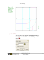
3.7. Blocking Strategy
With Hexa, the basic steps necessary to generate a hexahedral model are the same, regardless of model complexity. The blocking topology, once initialized, can then be modified by splitting and merging the blocks, as
well as through the use of an operation called O-grid (Refer to the next section). While these operations are
performed directly on the blocks, the blocks may also go through indirect modification by altering the sub-entities of the blocks (i.e.: the vertices, edges, faces).
Upon initialization, Hexa creates one block that encompasses the entire geometry. The subsequent operations
under the Blocking menu of developing the block model, referred to as "blocking the geometry," may be performed on a single block or across several blocks.
ANSYS ICEM CFD/AI*Environment 10.0 User Manual . . © SAS IP, Inc.
3–3
Chapter 3: Hexa
Note — Note : The topologic entities in Hexa are color-coded based on their properties.
Colors of Edges:
White Edges and Vertices:
These edges are between two material volumes. The edge and the associated vertices will be projected
to the closest CAD surface between these material volumes. The vertices of these edges can only move
on the surfaces.
Blue Edges and Vertices:
These edges are in the volume. The vertices of these edges, also blue, can be moved by selecting the
edge just before it and can be dragged on that edge.
Green Edges and Vertices:
These edges and the associated vertices are being projected to curves. The vertices can only be moved
on the curves to which it is being projected.
Red Vertices:
These vertices are projected to prescribed points.
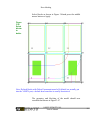
3.7.1. Split
The Split function, which divides the selected block interactively, may be applied across the entire block or to
an individual face or edge of a block by using the Split face or Split edge options, respectively. Blocks may be
isolated using the Index control.
3.7.2. Merge
The Merge function works similarly to split blocks; one can either merge the whole block or merge only a face
or an edge of the block.
While some models require a high degree of blocking skill to generate the block topology, the block topology
tools in Hexa allow the user to quickly become proficient in generating a complex block model.
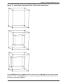
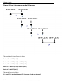
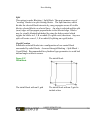
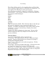
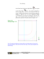
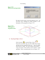
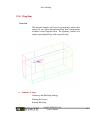
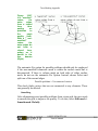
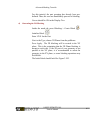
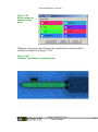
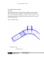
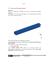
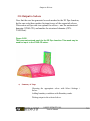
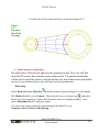
3.8. Using the Automatic O-grid
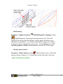
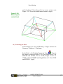
The O-grid creation capability is simply the modification of a single block or blocks to a 5 sub-block topology as
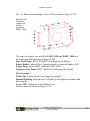
shown in Figure 3.1: “Initial block, block with O-Grid, O-Grid with include a face”. There are several variations of
the basic O-grid generation technique and the O-grid shown below is created entirely inside the selected block.
3–4
ANSYS ICEM CFD/AI*Environment 10.0 User Manual . . © SAS IP, Inc.
Section 3.8: Using the Automatic O-grid
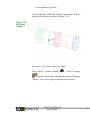
Figure 3.1 Initial block, block with O-Grid, O-Grid with include a face
Using the Add face option, an O-grid may also be created such that the O-grid passes through the selected
block faces. In Figure , the Add Face option was used on the right most block to add the bottom face on the
block prior to generating the O-grid.
ANSYS ICEM CFD/AI*Environment 10.0 User Manual . . © SAS IP, Inc.
3–5
Chapter 3: Hexa
Another important feature of the automatic O-grid is the ability to re-scale the O-grid after generation. When
the O-grid is generated, the size of the O-grid is scaled based upon a factor in the Blocking > O-grid parameter
window. The Re scale O grid option allows the user to re-scale the previously generated O-grid.
The blocks may also be modified by moving the vertices of the blocks and by defining specific relationships
between the faces, edges and vertices to the geometry.
3.9. Most Important Features of Hexa
Hexa has emerged as the quickest and most comprehensive software for generating large, highly accurate, 3Dgeometry based hexahedral meshes. Now, in the latest version of Hexa, it is also possible to generate 3D surface
meshes with the same speed and flexibility.
•
CAD- and projection-based hexahedral mesh generation
•
Easy manipulation of the 3D object-based topology model
•
Modern GUI and software architecture with the latest hexahedral mesh technology
•
Extensive solver interface library with over 100 different supported interfaces
•
Automatic O-grid generation and O-grid re-scaling
•
Geometry-based mesh size and boundary condition definition
•
Mesh refinement to provide adequate mesh size in areas of high or low gradients
•
Smoothing/relaxation algorithms to quickly yield quality meshes
•
Generation of multi-block structured, unstructured, and super- domain meshes
•
Ability to specify periodic definitions
•
Extensive replay functionality with no user interaction for parametric studies
•
Extensive selection of mesh bunching laws including the ability to graphically add/delete/modify control
points defining the graph of the mesh bunching functions
•
Link bunching relationships between block edges to automate bunching task
•
Topology operations such as translate, rotate, mirror, and scaling to simplify generation of the topology
model
•
Automatic conversion of 3D volume block topology to 3D surface mesh topology
•
Automatic conversion of 2D block topology to 3D block topology
•
Block face extrusion to create extended 3D block topology
•
Multiple projection options for initial or final mesh computation
•
Quality checks for determinant, internal angle and volume of the meshes
•
Domain renumbering of the block topology
•
Output block definition to reduce the number of multi-block structured output mesh files
•
Block orientation and origin modification options
3.10. Automatic O-grid generation
Generating O-grids is a very powerful and quick technique used to achieve a quality mesh. This process would
not have been possible without the presence of O-grids. The O-grid technique is utilized to model geometry
when the user desires a circular or "O"-type mesh either around a localized geometric feature or globally around
an object.
3–6
ANSYS ICEM CFD/AI*Environment 10.0 User Manual . . © SAS IP, Inc.
Section 3.12: Smoothing Techniques
3.10.1. Important Features of an O-grid
Generation of Orthogonal Mesh Lines at an Object Boundary
The generation of the O-grid is fully automatic and the user simply selects the blocks needed for O-grid
generation. The O-grid is then generated either inside or outside the selected blocks. The O-grid may be
fully contained within its selected region, or it may pass through any of the selected block faces.
Rescaling an O-grid After Generation
When the O-grid is generated, the size of the O-grid is scaled based upon the Factor in the Blocking > Ogrid parameter window. The user may modify the length of the O-grid using the Blocking > Re- scale Ogrid option. If a value that is less than 1 is assigned, the resulting O-grid will be smaller than the original. If,
however, a value is larger than 1, the resulting O-grid will be larger.
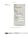
3.11. Edge Meshing Parameters
The edge meshing parameter task has been greatly automated by providing the user with unlimited flexibility
in specifying bunching requirements. Assigning the edge meshing parameters occurs after the development of
the block topology model. This option is accessible by selecting Meshing > Edge params.
The user has access to the following pre-defined bunching laws or Meshing laws:
Default (Bi-Geometric Law)UniformHyperbolicPoissonCurvatureGeometric 1Geometric 2Exponential 1Exponential 2Bi-ExponentialLinearSpline
The user may modify these existing laws by applying pre-defined edge meshing functions, accessible through
the Meshing > Edge Params > Graphs option in Hexa.
This option yields these possible functions: ConstantRampS curveParabola MiddleParabola EndsExponentialGaussianLinearSpline
Note — Note: By selecting the Graphs option, the user may add/delete/ modify the control points governing the function describing the edge parameter settings. Additional tools such as Linked Bunching
and the multiple Copy buttons provide the user with the ability to quickly apply the specified edge
bunching parameters to the entire model.
3.12. Smoothing Techniques
In Hexa, both the block topology and the mesh may be smoothed to improve the overall block/mesh quality
either in a certain region or for the entire model. The block topology may be smoothed to improve the block
shape prior to mesh generation. This reduces the time required for development of the block topology model.
The geometry and its associative faces, edges, and points are all constraints when smoothing the block topology
model. Once the block topology smoothing has been performed, the user may smooth the mesh after specifying
the proper edge bunching parameters.
The criteria for smoothing are: Determinant: This criteria attempts to improve the cell's determinant by movement
of nodes, which are subject to geometry and association constraints.Laplace: The Laplace option attempts to
minimize abrupt changes in the mesh lines by moving the nodes.Warp: The Warp method is based upon correcting the worst angle between two cells in the mesh. Quality: Like the determinant criteria, the Quality criteria
attempts to improve the cell's interior angle by repositioning the nodes, which are subject to geometry and association constraints.Orthogonality: The Orthogonality option attempts to provide orthogonal mesh lines at
all boundaries of the model.Skewness: The Skewness is defined differently for volume and surface cells. For a
volume cell, this value is obtained by taking all pairs of adjacent faces and computing the normals. The maximum
ANSYS ICEM CFD/AI*Environment 10.0 User Manual . . © SAS IP, Inc.
3–7
Chapter 3: Hexa
value thus obtained is normalized so that 0 corresponds to perpendicular faces, and 1 corresponds to parallel
faces. For surface cells, the skew is obtained by first taking the ratio of the two diagonals of the face. The skew
is defined as one minus the ratio of the shorter diagonal over the longer diagonal. Thus, 0 is perfectly rectangular,
and 1 represents maximum skewness.
3.13. Refinement and Coarsening
The refinement function, which is found through Meshing > Refinement, can be modified to achieve either a
refined or a coarsened result. The refinement/coarsening may be applied in all three major directions simultaneously, or they may be applied in just one major direction.
3.13.1. Refinement
The refinement capability is used for solvers that accept non-conformal node matching at the block boundaries.
The refinement capability is used to minimize the model size, while achieving proper mesh definition in critical
areas of high gradients.
3.13.2. Coarsening
In areas of the model where the flow characteristics are such that a coarser mesh definition is adequate,
coarsening of the mesh may be appropriate to contain model size.
3.14. Replay Functionality
Parametric changes made to model geometry are easily applied through the use of Hexa's replay functionality,
found in File > Replay. Changes in length, width and height of specific geometry features are categorized as
parametric changes. These changes do not, however, affect the block topology. Therefore, the Replay function
is capable of automatically generating a topologically similar block model that can be used for the parametric
changes in geometry.
If any of the Direct CAD Interfaces are used, all geometric parameter changes are performed in the native CAD
system.
3.14.1. Generating a Replay File
The first step in generating a Replay file is to activate the recording of the commands needed to generate the
initial block topology model. As mentioned above, this function can be invoked through File > Replay. All of
the steps in the mesh development process are recorded, including blocking, mesh size, edge meshing,
boundary condition definition, and final mesh generation. The next step in the process is to make the parametric
change in the geometry and then replay the recorded Replay file on the changed geometry. All steps in the
mesh generation process are automated from this point.
3.14.2. Advantage of the Replay Function
With the Replay option, the user is capable of analyzing more geometry variations, thus obtaining more information on the critical design parameters. This can yield optimal design recommendations within the project time
limits.
3.15. Periodicity
Periodic definition may be applied to the model in Hexa. The Periodic nodes function, which is found under
Blocking > Periodic nodes, plays a key role in properly analyzing rotating machinery applications, for example.
3–8
ANSYS ICEM CFD/AI*Environment 10.0 User Manual . . © SAS IP, Inc.
Section 3.16: Mesh Quality
Typically, the user will model only a section of the rotating machinery, as well as implement symmetry, in order
to minimize the model size. By specifying a periodic relationship between the inflow and outflow boundaries,
the particular specification may be applied to the model -- flow characteristics entering a boundary must be
identical to the flow characteristics leaving a boundary.
3.15.1. Applying the Periodic Relationship
The periodic relationship is applied to block faces and ensures that a node on the first boundary have two
identical coordinates to the corresponding node on the second boundary. The user is prompted to select corresponding vertices on the two faces in sequence. When all vertices on both flow boundaries have been selected,
a full periodic relationship between the boundaries has been generated.
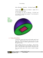
3.16. Mesh Quality
The mesh quality functions are accessible through Meshing > Quality check. Any of the four quality check options
will display a histogram plot for the user.
3.16.1. Determining the Location of Cells
By clicking on any of the histogram bars with the left button, the user may determine where in the model these
cells are located. The selected histogram bars will change in color to pink. After selecting the bar(s), the Show
button is pressed to highlight the cells in this range. If the Solid button is turned on, the cells marked in the
histogram bars will be displayed with solid shading.
3.16.2. Determinant
The Determinant check computes the deformation of the cells in the mesh by first calculating of the Jacobian
of each hexahedron and then normalizing the determinant of the matrix. A value of 1 represents a perfect
hexahedral cube, while a value of 0 is a totally inverted cube with a negative volume. The mesh quality, measured
on the x-axis, of all cells will be in the range from 0 to1. If the determinant value of a cell is 0, the cube has one
or more degenerated edges. In general, determinant values above 0.3 are acceptable for most solvers.
The y-axis measures the number of cells that are represented in the histogram. This scale ranges from 0 to a value
that is indicated by the Height. The subdivision among the quality range is determined by the number of assigned
Bars.
3.16.3. Angle
The Angle option checks the maximum internal angle deviation from 90 degrees for each cell. Various solvers
have different tolerance limits for the internal angle check. If the cells are distorted and the internal angles are
small, the accuracy of the solution will decrease. It is always wise to check with the solver provider to obtain
limits for the internal angle threshold.
3.16.4. Volume
The Volume check will compute the internal volume of the cells in the model. The units of the volume will be
displayed in the unit that was used to create the model.
3.16.5. Warpage
The Warpage check will yield a histogram that indicates the level of cell distortion. Nodes that are in-plane with
one another will produce a cell with small warpage. Nodes that make cells twisted or distorted will increase a
ANSYS ICEM CFD/AI*Environment 10.0 User Manual . . © SAS IP, Inc.
3–9
Chapter 3: Hexa
cells distortion, giving a high degree of warpage. The y-axis is the scale for the number of cells represented in
the histogram - a value determined by the assigned Height. The x- axis, which ranges from a Min of 0 to a Max
of 90, is the degree of warpage that a cell experiences.
3–10
ANSYS ICEM CFD/AI*Environment 10.0 User Manual . . © SAS IP, Inc.
Chapter 4: Properties
Properties menu allows the user to create different materials by specifying the material type that is whether
isotropic, Young's Modulus, Poission's ratio. Once the material is created the user can apply those properties to
the respected elements.
4.1. Create Material Property
Here the user can define a material by Specifying a name of the material, define whether isotropic, Young's
Modulus, Shear modulus, Poission's ratio, Mass Density, Thermal expansion coefficient.
4.2. Save Material
This Option allows the user to save the material which is created, So that user can retrieve the material when
ever necessary. The material file will be saved with .mat extension.
4.3. Open Material
This option allows the user to open a material file so that the user can use the same for future or modify the file
and save for further usage.
4.4. Define Table
Here user can create different tables by specifying the values for x and y ,and user can even visualize the graph.
4.5. Define Point Element
Although the user has created the mesh, user has to apply the material created to the respected elements. Allows
user to define point element, user have to specify Mass type and scalar Mass.
4.6. Define Line Element
This option allows the user to select a part and Specify the material which is already, and property identification
number, cross section Area and moment of inertia.
4.7. Define Shell Element
This option allows the user to select a part and specify the property identification number material, thickness
etc.
4.8. Define Volume Element
This option allows the user to select a part and specify the material, property identification number etc.
ANSYS ICEM CFD/AI*Environment 10.0 User Manual . . © SAS IP, Inc.
4–2
Chapter 5: Constraints
Here user can define the constraints on deferent entities like point, curve, surface, subset & other options like
Contact definition, Velocity and Rigid Wall.
5.1. Displacement on Point
This option allows the user to apply the constraint on point in directional displacement Translation can be constrained in all the three directions by clicking in the checkbox displacement values can be specified, and similarly
Rotational displacement.
5.2. Displacement on Curve
This option allows the user to apply the constraint on Curve in directional displacement Translation can be
constrained in all the three directions, and similarly rotational displacement
5.3. Displacement on Area
This option allows the user to apply the constraint on Area in directional displacement as well as Rotational displacement
5.4. Displacement on Subset
This option allows the user to apply the constraint on Subset in directional displacement as well as Rotational
displacement
5.5. Define Contact
Here there are two options are available for the user
5.5.1. Automatic Detection
User has to specify Contact proximity Factor, It is a range within which all the elements get selected.
5.5.2. Manual Definition
Here user has to manually pick the contact and target surfaces. for the contact creation.
5.6. Define Single Surface Contact
This is mainly used for LS-Dyna Solver, wherein user can pick the contact surface.
5.7. Define Initial velocity
This allows the user to define the rigid wall by specifying the directional and rotational velocity.
5.8. Define Planar Rigid wall
User can define Planar Rigid Wall by Specifying the Head and Tail coordinates.
ANSYS ICEM CFD/AI*Environment 10.0 User Manual . . © SAS IP, Inc.
5–2
Chapter 6: Loads
In this tab there are several optional available for applying the Load, Pressure temperature and gravity
Theory
Force Distribution follows the following formulation.
Curve
Total Force 'FT' is applied on the curve as shown in Figure 6.1: “ Elements on Curve”.
Where L1 is the length of Element 1, '0' and '1' are the node number connecting Element 1.
Figure 6.1 Elements on Curve
Then the force distribution on 'Linear' elements as per the FEA concept is shown in Figure 6.2: “Force Distribution
as per the FEA concepts”.
ANSYS ICEM CFD/AI*Environment 10.0 User Manual . . © SAS IP, Inc.
Chapter 6: Loads
Figure 6.2 Force Distribution as per the FEA concepts
The formulation for Linear Element is as follow
Points 0: F0 = 0.5* FT *(L1/LT)
Points 1: F1 = 0.5* FT *(L1/LT) + 0.5* FT *(L2/LT)
Points 2: F2 = 0.5* FT *(L2/LT) + 0.5* FT *(L3/LT)
Points 3: F3 = 0.5* FT *(L3/LT) + 0.5* FT *(L4/LT)
Points 4: F4 = 0.5* FT *(L4/LT)
The general formula is as follow
Fi = Sum [FT * (L (attached element)/LT) * (1/number of nodes per element)]
6–2
ANSYS ICEM CFD/AI*Environment 10.0 User Manual . . © SAS IP, Inc.
If we sum up F0+F1+F2+F3+F4 then the resultant comes to be FT
It also satisfies the FEA concepts
Now if we want to apply the same force on the Quadratic Element as shown in Figure 6.3: “Quadratic Element
Nodes position”.
Figure 6.3 Quadratic Element Nodes position
The Load distribution as per the FEA concept on the Quadratic elements is shown in Figure 6.4: “Load Distribution
as per the FEA concepts”.
ANSYS ICEM CFD/AI*Environment 10.0 User Manual . . © SAS IP, Inc.
6–3
Chapter 6: Loads
Figure 6.4 Load Distribution as per the FEA concepts
The formulation of Total Force at the side nodes is as follow
Points 0:F0q = (1/6)* FT *(L1/LT)
Points 1:F1q = (1/6)* FT *(L1/LT) + (1/6)* FT *(L2/LT)
Points 2:F2q = (1/6)* FT *(L2/LT) + (1/6)* FT *(L3/LT)
Points 3:F3q = (1/6)* FT *(L3/LT) + (1/6)* FT *(L4/LT)
Points 4: F4q = (1/6)* FT *(L4/LT)
But the formulation of mid-side node is as follow
Points m1: Fm1 = (2/3)* FT *(L1/LT)
Points m2: Fm2 = (2/3)* FT *(L2/LT)
6–4
ANSYS ICEM CFD/AI*Environment 10.0 User Manual . . © SAS IP, Inc.
Points m3: Fm3 = (2/3)* FT *(L3/LT)
Points m4: Fm4 = (2/3)* FT *(L4/LT)
As in the previous case of Linear Element the total Force of Quadratic element is
FTotal= F0q+ F1q+ F2q+ F3q+ F4q+ Fm1+ Fm2+ Fm3+ Fm4
Which yields FTotal=FT
QUAD 9 Consistent Nodal Load Distributions
The Nine Node two dimension Lagrange QUAD 9 Element is shown in Figure 6.5: “QUAD9 Element”.
Figure 6.5 QUAD9 Element
The Shape function for Corner Node
N1 (?, ?) = (1/4)* ??(?-1)(?-1)
The Shape function for Mid-Side Node
N5(?, ?) = (1/2)* ?(1-?2)( ?-1)
The Shape function for Middle Node
N9(?, ?) = (1-?2)(1-?2)
Suppose a Force F is uniformly distributed over the whole Area the pressure is
p=F/4 (Because in ‘??' coordinate system the Area of the rectangle is '4')
To Find Consistent Load
ANSYS ICEM CFD/AI*Environment 10.0 User Manual . . © SAS IP, Inc.
6–5
Chapter 6: Loads
Consistent Load at Node 1=L1
Consistent Load at Node 5=L5
Consistent Load at Node 9=L9
On Integration we get the following values
L1=p ?=-1? ?= + 1?=-1? ?= + 1N1 d?d?=4p/36
L5=p ?=-1? ?= + 1?=-1? ?= + 1N5 d?d?=4p/9
L9=p ?=-1? ?= + 1?=-1? ?= + 1N9 d?d?=16p/9
Now F=4p
Putting this value in the above equation we get the consistent Nodal Force as
L1=F/36
L5=F/9
L9=4F/9
By symmetry Consistent Nodal Force on Node 1, 2, 3&4 are equal.
By symmetry Consistent Nodal Force on Node 5, 6, 7&8 are equal.
Now Total Force =4*L1+4*L5+L9
=F/9+4F/9+4F/9
=F
Note — Note: The same method is employed for calculating the Consistent Nodal Force on QUAD8 element, which gives correct results
6.1. Force on Point
Using this option user can apply force on points in all the three directions as well as user can apply the moment
in x,y,z, directions. Here specifying negative value implies force applied in the negative direction.
6.2. Force on curve
Using this option user can apply force on Curves in all the three directions as well as user can apply the moment
about x, y, z directions.
There are two options available Force can be applied on curves uniformly -implies the nodes attached to the
curve will be applied the same force
Incase of Total, The force applied on the curve gets distributed on the nodes attached to the curves according
to the FEA concepts
6–6
ANSYS ICEM CFD/AI*Environment 10.0 User Manual . . © SAS IP, Inc.
Section 6.12: Set Gravity
6.3. Force on Surface
Using this option user can apply force on Surface in all the three directions; Negative value indicates force acts
away from the surface.
6.4. Force on Subset
Using this option user can apply Force on Subset.
6.5. Pressure on surfaces
The user can apply the Pressure on Surfaces.
6.6. Pressure on subset
The user can apply the Pressure on Subset.
6.7. Temperature on Points
This option allows the user to apply the Temperature on point.
6.8. Temperature on curves
This option allows the user to apply the Temperature on Curve.
6.9. Temperature on Surface
Allows user to apply Temperature on Surface
6.10. Temperature on Body
Allows user to apply Temperature on Body
6.11. Temperature on Subset
This option allows the user to apply the Temperature on Subset
6.12. Set Gravity
This option allows the user to apply the Gravity
ANSYS ICEM CFD/AI*Environment 10.0 User Manual . . © SAS IP, Inc.
6–7
6–8
Chapter 7: Solver Options
This Menu includes tabs for specifying the Solver. Specify the analysis Solution and Post processing
Fore more useful information about Solver Options, please go to http://www-berkeley.ansys.com/faq/faq_topic_7.html.
7.1. Setup Solver Parameters.
You can select from the following solvers: ANSYS, Nastran, ABAQUS, and LSDyna.
7.2. Setup Analysis Type
Depending on the selected solver, different options are available. For the ANSYS solver, you can select either
Structural or Thermal. If Nastran solver is selected, then you have the choice of more Analysis types.
7.3. Setup Sub-Case
To apply the load in different steps, subcases can be created.
7.4. Write/View Input file
To create and view the input file generated for the solver.
7.5. Submit Solver Run
Using this option, you can solve the input file generated for a particular solver.
7.6. Post Process Results
Allows you to plot the results.
7.7. FEA Solver Support
For more useful information on FEA Solvers Support, please go to http://www-berkeley.ansys.com/faq/faq_topic_7.html
ANSYS ICEM CFD/AI*Environment 10.0 User Manual . . © SAS IP, Inc.
ANSYS ICEMCFD 10.0
Tutorial Manual
August 2005
Table of Contents
1: Introduction to ANSYS ICEMCFD
1
1.1: The Unified Geometry Concept
2
1.2: The ANSYS ICEMCFD Geometry Interface
3
1.3: Meshing Modules
4
1.4: Mesh Visualization and Optimization
6
2: ANSYS ICEMCFD GUI
8
2.1: Main Menu
9
2.2: Utilities
10
2.3: Function Tabs
10
2.3.1: The Geometry menu
10
2.3.2: The Mesh menu
11
2.3.3: The Blocking menu
11
2.3.4: The Edit Mesh menu
12
2.3.5: The Output menu
12
2.3.6: The Post Processing menu
13
2.4: The Display Control Tree
13
2.4.1: Geometry
14
2.4.2: Mesh
14
2.4.3: Parts
14
2.4.4: The Message window
14
2.5: The Histogram window
15
3: CFD Tutorials
16
3.1: Geometry Creation
16
3.1.1: 2D Pipe Junction
16
3.1.2: 3D Pipe Junction
31
ANSYS ICEMCFD 10.0
Tutorial Manual
iii
3.1.3: Sphere Cube
43
3.1.4: Pipe Blade
55
3.2: Hexa Meshing
66
3.2.1: Introduction
66
3.2.2: 2D Pipe Junction
78
3.2.3: 2D Car
109
3.2.4: 3D Pipe Junction
139
3.2.5: Sphere Cube
167
3.2.6: Pipe Blade
182
3.2.7: Elbow Part
220
3.2.8: Wing Body
249
3.3: Hexa Meshing Appendix
276
3.3.1: The Most Important Features of Blocking
276
3.3.2: Automatic O-grid Generation
277
3.3.3: Important Features of an O-grid
277
3.3.4: Edge Meshing Parameters
278
3.3.5: Smoothing Techniques
279
3.3.6: Refinement and Coarsening
280
3.3.7: Replay Functionality
281
3.3.8: Periodicity
282
3.3.9: Mesh Quality
282
3.4: Tetra
285
3.4.1: Introduction
285
3.4.2: Sphere Cube
292
3.4.3: 3D Pipe Junction
306
3.4.4: Fin Configuration
327
ANSYS ICEMCFD 10.0
Tutorial Manual
iv
3.4.5: Piston Valve
341
3.4.6: STL Configuration
356
3.5: Tetra Meshing Appendix
382
3.5.1: Mesh Editor - Before Creating the Tetra Mesh
382
3.5.2: Tetra
385
3.5.3: Editing the Tetra Mesh
387
3.6: Advanced Meshing Tutorials
398
3.6.1: Hexa Mesh in a Grid Fin
399
3.6.2: Hybrid tube
451
3.6.3: Tetra mesh for Submarine
480
3.6.4: Quad Mesh on a Frame
491
3.6.5: STL Repair with Tetra meshing
508
3.6.6: Workbench Integration
526
3.7: Cart3D
557
3.7.1: Tutorial Three Plugs
558
3.7.2: Tutorial Opera M6 Wing with 0.54 M
569
3.7.3: Onera M6 Wing with 0.84 M
590
3.7.4: Supersonic Missile
611
3.7.5: Business Jet
652
3.7.6: Bomber
670
3.7.7: Advanced Pitot Intake Tutorial
693
3.7.8: Advanced Tutorial Converging-Diverging Nozzle flow
715
3.8: Output to Solvers
735
3.8.2: Unstructured Mesh
737
3.8.3: Structured Mesh
747
3.9: Post Processing Tutorials
752
ANSYS ICEMCFD 10.0
Tutorial Manual
v
3.9.1: Pipe Network
752
3.9.2: Pipe Network (Advanced)
769
3.9.3: Space Shuttle
785
3.9.4: Space Shuttle (Advanced)
797
4: FEA Tutorials
807
4.1: Ansys Tutorial
807
4.1.1: T-Pipe: Modal Analysis
807
4.1.2: Connecting Rod: Thermal Boundary Condition
823
4.1.3: Contact Analysis
861
4.1.4: PCB-Thermal Analysis
893
4.2: LS-Dyna Tutorial
916
4.2.1: Frame: Quasi-Static Analysis
916
4.2.2: Front Door-Side Impact
935
4.2.3: PDA Drop Impact
952
4.3: Nastran Tutorial
976
4.3.1: T-Pipe
976
4.3.2: Bar
1013
4.3.3: Frame
1045
4.3.4: Connecting Rod
1088
4.3.5: Hood
1119
5: ANSYS ICEMCFD - CFX Tutorials
5.1: Static Mixer
1136
1136
5.1.1: Overview
1136
5.2: Static Mixer 2 (Refined Mesh)
5.2.1: Overview
1163
1163
5.3: Blunt Body
1177
ANSYS ICEMCFD 10.0
Tutorial Manual
vi
5.3.1: Overview
1177
5.4: Heating Coil
1200
5.4.1: Overview
1200
ANSYS ICEMCFD 10.0
Tutorial Manual
vii
The ANSYS ICEMCFD Projects
Each project represents a directory within the
$ICEM_ACN/../docu/CFDHelp/CFD_Tutorial_Files directory. Since
some of the projects are used as examples in multiple meshing modules,
this directory may contain several files. A particular project directory can
contain one or more of the following files:
*.prj:
Project settings
*.tin:
Tetin (geometry)
*.uns:
Unstructured mesh
domain.*: Multiblock structured hexahedral meshes
*.blk:
Block topology
*.fbc:
Boundary conditions (for solver output)
*.atr:
Attributes (for solver output)
*.par:
Parameters (for solver output)
*.rpl:
Replay script
*.jrf:
Journal (echo) file
These extensions are preceded typically with the project name, e.g.,
project1.tin is the tetin (geometry) file associated with project1. Most of
the tutorials will already have a tetin file called geometry.tin (the project
has yet to be created).
Some of the tutorials will begin with a 3rd party geometry, e.g.,
geometry.stl (stereolithography – triangulated surface data), which is then
saved to the *.tin format.
ANSYS ICEMCFD 10.0
Tutorial Manual
8
The Tutorial Examples
It is recommended that for each chapter, the tutorials be done in sequence.
Commands in succeeding tutorials may be referred to or explained in a
previous tutorial. Please read through the introduction before beginning
the tutorials.
The input files for the tutorials can be found within the ANSYS
ICEMCFD installation. For example:
~/Ansys_inc/v100/icemcfd/linux64/../docu/CFDHelp/CFD_Tutorial_Files.
They can also be downloaded from http://wwwberkeley.ansys.com/icemcfd_ftp/index.html#icemcfd_100_manual. This
download also contains these manuals in *.pdf format for hardcopy output.
Tutorial Design
These tutorials provide explanation for each step in the mesh generation
process. The user not only learns the sequence of commands, but also
comes to understand the concept behind the individual commands. After
going through these tutorials, the user will be capable of extending his or
her knowledge of the functions into more complicated projects.
Each example will either introduce new features or use familiar features in
new ways to ultimately achieve better results for specific geometries.
Lessons begin by outlining the functions and operations being introduced
in the example. New features will receive the most thorough explanations
in the chapter in which they are first introduced.
For specific questions regarding the usage of a command, refer to Help >
Help Topics.
Text Conventions
The text conventions of this tutorial are categorized in the following
manner:
ANSYS ICEMCFD 10.0
Tutorial Manual
9
“>” indicates order of selection. For example, “Edges > Group curve > screen
select” means to choose the screen select option of the Group curve function
found in the Edges menu.
Italicized font indicates a button selection.
Bold font indicates user input.
ALL CAPS indicates a part/entity name.
Mouse and Keyboard functions
Mouse Button or
Action Description
Keyboard key
Left mouse button,
Rotates model
click and drag
Right mouse button,
Zooms in or out on the
click and drag
model
up/down
Right mouse button,
Rotates model about
click and drag
screen Z-axis
left/right
Press F9, and then use Toggles temporarily to
any mouse button.
dynamic mode
Press F9 again to
(translate, zoom,
return to previous
rotate)
operation.
F11 Key
Emergency Graphics
Reset
ANSYS ICEMCFD 10.0
Tutorial Manual
10
Introduction to ANSYS ICEMCFD
1: Introduction to ANSYS ICEMCFD
Meeting the requirement for integrated mesh generation and post
processing tools for today’s sophisticated analysis, ANSYS ICEMCFD
provides advanced geometry acquisition, mesh generation, mesh
optimization, and post-processing tools.
Maintaining a close relationship with the geometry during mesh
generation and post-processing, ANSYS ICEMCFD is used especially in
engineering applications such as computational fluid dynamics and
structural analysis.
ANSYS ICEMCFD’s mesh generation tools offer the capability to
parametrically create meshes from geometry in numerous formats:
Multiblock structured
Unstructured hexahedral
Unstructured tetrahedral
Cartesian with H-grid refinement
Hybrid Meshes comprising hexahedral,
pyramidal and/or prismatic elements
tetrahedral,
Quadrilateral and triangular surface meshes
ANSYS ICEMCFD provides a direct link between geometry and
analysis.
In ANSYS ICEMCFD, geometry can be input from just about any format,
whether it is from a commercial CAD design package, 3rd party universal
database, scan data or point data.
Beginning with a robust geometry module which supports the creation and
modification of surfaces, curves and points, ANSYS ICEMCFD’s open geometry
ANSYS ICEMCFD 10.0
Tutorial Manual
1
Introduction to ANSYS ICEMCFD
database offers the flexibility to combine geometric information in various
formats for mesh generation. The resulting structured or unstructured meshes,
topology, inter-domain connectivity and boundary conditions are then stored in a
database where they can easily be translated to input files formatted for a
particular solver.
1.1: The Unified Geometry Concept
The unified geometry input environment in ANSYS ICEMCFD provides
rapid geometry evaluation capability for computational mesh generation.
This environment can combine CAD surface geometry and triangulated
surface data into a single geometry database using the geometry interfaces.
All geometry entities, including surfaces, curves and points are tagged or
associated to a grouping called a part. With this part association, the user
can quickly toggle off or on all entities within the parts, visualize them
with a different color, assign mesh sizes on all entities within the part and
apply different boundary conditions by part.
Geometry is collected into a common geometry database (tetin file) which
can be used by any of ANSYS ICEMCFD’s meshing modules.
Direct CAD Interfaces and Intelligent Geometry
The ANSYS ICEMCFD Direct CAD Interfaces provide the bridge between
parametric geometry creation tools available in CAD systems and the
computational mesh generation, post-processing and mesh optimization tools
available in ANSYS ICEMCFD, allowing users to operate in their native CAD
systems. ANSYS ICEMCFD currently supports Direct CAD Interfaces for:
Catia
I-deas
Pro/E
Unigraphics
Solid Works
ANSYS ICEMCFD 10.0
Tutorial Manual
2
Introduction to ANSYS ICEMCFD
In an environment that has the look and feel of their native CAD system, users
can choose solids, surfaces, curves and points, group these entities into parts and
assign mesh sizes for mesh generation.
Further information on ANSYS ICEMCFD’s Direct CAD Interfaces is available
in the ANSYS ICEMCFD Direct CAD Interface Tutorial Manual.
Since the CAD geometry is tagged with mesh parameters and boundary
conditions directly in this interface, the user can recalculate a mesh reflecting
these changes in the geometry immediately after having saved the geometry file.
3rd Party Interfaces
Available for STEP/IGES, DXF, GEMS, ACIS, DWG, Parasolid and point data.
Triangulated Surface Data Input
Available for STL, Patran, Nastran, Plot3d (a popular Aerospace format for
multiblock structured surface meshes) and VRML.
1.2: The ANSYS ICEMCFD Geometry Interface
Geometry Tools
ANSYS ICEMCFD includes a wide range of tools for creating new and/or
manipulating existing geometry. This allows the user to alter complex
geometry or create simple geometry without having to go back to the
original CAD. This can be done for CAD (NURBS surfaces) and
triangulated surface data.
Although most of the meshing modules within ANSYS ICEMCFD are
forgiving of minor gaps and holes in the geometry, in some cases it is
necessary to find and close large gaps and holes without returning back to
the original CAD. ANSYS ICEMCFD provides tools to do both on either
CAD or triangulated surfaces.
ANSYS ICEMCFD 10.0
Tutorial Manual
3
Introduction to ANSYS ICEMCFD
Finally, curves and points can be automatically created to capture certain
key features in the geometry. These curves and points will act as
constraints for the mesher, forcing nodes and edges of the elements to lie
along them, and thus capturing the hard feature.
1.3: Meshing Modules
Tetra/Auto Volume
ANSYS ICEMCFD Tetra takes full advantage of object-oriented
unstructured meshing technology. With no tedious up-front triangular
surface meshing required providing well-balanced start meshes, ANSYS
ICEMCFD Tetra works directly from the CAD surfaces and fills the
volume with tetrahedral elements using the Octree approach. A powerful
smoothing algorithm provides the element quality. Options are available to
automatically refine and coarsen the mesh both on geometry and within
the volume.
A Delauny algorithm is also included to create tetras from surface mesh
that already exists and also to give a smoother transition in the volume
element size.
Hexa
This ANSYS ICEMCFD semi-automated meshing module presents rapid
generation of multi-block structured or unstructured hexahedral volume
meshes.
ANSYS ICEMCFD Hexa represents a new approach to grid generation
where the operations most often performed by experts are automated and
made available at the touch of a button.
Blocks can be built and interactively adjusted to the underlying CAD
geometry. This blocking can be used as a template for other similar
geometries for full parametric capabilities. Complex topologies, such as
internal or external O-grids can be generated automatically.
ANSYS ICEMCFD 10.0
Tutorial Manual
4
Introduction to ANSYS ICEMCFD
Prism
For better modeling of near-wall physics of the flow field, ANSYS
ICEMCFD Prism generates hybrid tetrahedral grids consisting of layers of
prism elements near the boundary surfaces and tetrahedral elements in the
interior. Compared to pure tetrahedral grids, this results in smaller analysis
models, better convergence of the solution and better analysis results.
Hybrid Meshes
Hybrid meshes can be created by several means:
Tetra and Hexa meshes can be united (merged) at a common interface in
which a layer of pyramids are automatically created at a common interface
to make the two mesh types conformal. Good for models where in one
part it is desired to have a “structured” hexa mesh and in another more
complex part it is easier to create an “unstructured” tetra mesh.
Hex core meshes can be generated where the majority of the volume is
filled with a Cartesian array of hexahedral elements essentially replacing
the tetras. This is connected to the remainder of a prism/tetra hybrid by
automatic creation of pyramids. Hex core allows for reduction in number
of elements for quicker solver run time and better convergence.
Shell Meshing
ANSYS ICEMCFD provides a method for rapid generation of surface
meshes (quad and tri), both 3D and 2D. Mesh types can be all quad, quad
dominant or all tri. Three methods are available:
Patch based shell meshing: Uses a series of “loops” which are
automatically defined by the boundaries of surfaces and/or a series of
curves. Gives best quad dominant quality and capturing of surface details
ANSYS ICEMCFD 10.0
Tutorial Manual
5
Introduction to ANSYS ICEMCFD
Patch independent shell meshing: Uses the Octree method. Best and most
robust on unclean geometry.
Mapped based shell meshing: Internally uses a series of 2d blocks, results
in mesh better lined up with geometry curvature.
1.4: Mesh Visualization and Optimization
Mesh visualization tools, including solid/wireframe display, 2D cut
planes, color coding and node display is provided.
After initial mesh is created by any of the meshing modules, diagnostics
can be performed to determine local and overall mesh quality. Automatic
smoothing algorithms are in place to improve overall quality. Local
editing can be done using a wide range of automatic re-meshing and
manual mesh editing tools.
Output Interfaces
ANSYS ICEMCFD includes output interfaces to over 100 flow and
structural solvers, producing appropriately formatted files that contain
complete mesh and boundary condition information.
Post Processing
ANSYS ICEMCFD Visual3 provides easy-to-use powerful result
visualization features for structured, unstructured and hybrid grids, both
steady-state and transient.
Visual3 integrates CAD Geometry, computational grids and the flow
solution within one environment. It provides an in-depth view of data
with visualization tools such as cut planes, stream ribbons, contours,
vectors, grids, iso-surfaces, offset surfaces, result surfaces, integration, XY
plots, data probes, function calculator, solution and experimental
comparison, scripts, annotations and animation. Results can be
ANSYS ICEMCFD 10.0
Tutorial Manual
6
Introduction to ANSYS ICEMCFD
interpolated on imported surface meshes and written out to a different
solution process, e.g. interpolating fluid results on to a surface mesh and
brought in as loads for a structural analysis.
A surface manager tool controls the display status for all surfaces,
including any dynamic surface, domain surfaces and user-defined
surfaces.
ANSYS ICEMCFD 10.0
Tutorial Manual
7
ANSYS ICEMCFD GUI
2: ANSYS ICEMCFD GUI
ANSYS ICEMCFD’s unified graphical user interface, also known as
AI*Environment, offers a complete environment to create and edit your
computational grids.
The AI*Environment GUI includes the following:
Main menu
Function Tabs
Utility icons
Data Entry Zone
Display Control Tree
Graphics Window
Message Window
Histogram (Quality) Display Window
Selection Toolbar
Figure 2.1
The ICEM CFDMesh Editor
ANSYS ICEMCFD 10.0
Tutorial Manual
8
ANSYS ICEMCFD GUI
2.1: Main Menu
Many of the following menu items are accessible as icons in the upper left
hand corner.
File
The File menu is used to create new or open existing projects, loading and
saving files, importing and exporting geometries and initialize scripting.
Edit
This menu contains Undo/Redo, the option to open a shell window, and
various internal mesh/geometry conversion commands.
View
Contains various options for the standard view, controls, and annotations.
Info
This menu allows the user to get various information regarding geometry,
mesh and individual entities.
Settings
ANSYS ICEMCFD 10.0
Tutorial Manual
9
ANSYS ICEMCFD GUI
Contains default settings for performance, graphics, and other settings
most likely to be used more than 90% of the time by a specific user.
Help
Contains links to reference material, tutorials, user’s guide and version
information.
2.2: Utilities
Icon representation of some of the most commonly used functions
represented in the Main menu including opening/closing a project,
undo/redo, and display options. It also includes measurement and setup of
local coordinate systems.
2.3: Function Tabs
The main functionality for the entire grid generation process is accessed
through the function tabs which include: Geometry, Mesh, Blocking,
Edit mesh, Output, Post-processing.
2.3.1: The Geometry menu
The Geometry menu includes functions for the creation, editing and repair
of geometry.
For more information on ANSYS ICEMCFD’s Tetin files and treatment of
geometry entities, refer to the section on Geometry definitions in Help >
Help Topics.
Functions and utilities in this menu include:
Create Point
Create/Modify Curve
Create/Modify Surface
Create Body
Create Faceted
Repair Geometry
Transform Geometry
Restore Dormant Entities
ANSYS ICEMCFD 10.0
Tutorial Manual
10
ANSYS ICEMCFD GUI
Delete Point, Delete Curve, Delete Surface, Delete Body and Delete Any
Entity.
2.3.2: The Mesh menu
These tools are the heart of ANSYS ICEMCFD. The Mesh menu contains
the ANSYS ICEMCFD meshing modules as well as options to set mesh
sizes (parameters).
Depending on the licensing, some users may not be able to access certain
meshing modules. Contact customer support or ANSYS ICEMCFD’s
website for guidance with any licensing questions, or for help with adding
any additional modules to the license.
The following buttons would lead to different mesh generation modules,
which ANSYS ICEMCFD maintains and develops:
Set Global Mesh Size
Set Surface Mesh Size
Set Curve Mesh Size
Set Meshing Params by Part
Create Mesh Density
Create Elements
Surface Meshing
Volume Meshing
Mesh Prism
Global Cartesian Mesher
Extrude Mesh.
Pressing any of these buttons will invoke the preferred meshing module.
2.3.3: The Blocking menu
The Blocking menu contains the functions necessary to create a topology
for block structured hexahedral meshes. Either a block file must be loaded
or an initial block created to make all the items active.
Create Block
Split Block
Merge Vertices
ANSYS ICEMCFD 10.0
Tutorial Manual
11
ANSYS ICEMCFD GUI
Edit Block
Associate
Move Vertex
Transform Blocks
Edit Edge
Pre-Mesh Params
Pre-Mesh Quality
Pre-Mesh Smoothing
Block Checks
Delete Block
2.3.4: The Edit Mesh menu
The Edit mesh menu contains tools necessary for mesh editing, both
automated and manual. Operations include:
Create Elements
Check Mesh
Display Mesh Quality
Smooth Mesh Globally
Smooth Hexahedral Mesh Orthogonal
Repair Mesh
Merge Nodes
Split Mesh
Move Nodes
Transform Mesh
Convert Mesh Type
Adjust Mesh Density
Renumber Mesh
Reorient Mesh
Delete Nodes
Delete Elements
2.3.5: The Output menu
The Output menu contains all tools necessary for setting up the model and
writing out to the solver:
Select Solver
ANSYS ICEMCFD 10.0
Tutorial Manual
12
ANSYS ICEMCFD GUI
Boundary Conditions
Edit Parameters
Write Input
2.3.6: The Post Processing menu
The Post Processing menu controls the viewing of solution results. A
results file (from various CFD and structural formats) must first be loaded
to make this menu active. The functions included in the post processing
menu are:
Set Transient Time
Variables
Define Cut Plane
Define Iso Surface
Point Probe on Surface
Import External Surface
Streams
Control All Animations
Annotation
XY or polar
2.4: The Display Control Tree
The Display Control Tree, also referred to as the Display tree, along the
lower left side of the screen, allows control of the display by part,
geometric entity, element type and user-defined subsets.
The tree is organized by categories. Each category can be turned on or off
by selecting the check box. If the check mark is faded, some of the subcategories are turned on and some off. Each category can be expanded by
selecting the “+” symbol to reveal the sub-categories. Select “-“ to
collapse the tree.
Since some functions are performed only on the entities shown, the model
tree is a very important feature to use when isolating the particular entities
to be modified.
Right mouse selecting a particular category or type will reveal several
display and modification options.
ANSYS ICEMCFD 10.0
Tutorial Manual
13
ANSYS ICEMCFD GUI
2.4.1: Geometry
Controls display of points, curves, surfaces and bodies (material volumes).
Subsets can also be created, displayed and modified. A given subset can
contain any number of different geometry types. A given entity can
belong to more than one subset.
2.4.2: Mesh
Controls display of all mesh types: points (node elements), lines (bars),
shells (tris or quads) and volumes (tetras, pyramids, prisms, hexas).
Subsets within this category are the same as for Geometry but contain only
mesh element types.
2.4.3: Parts
All entities, geometry or mesh, are associated to a given part. An entity
cannot belong to more than one part. With this association, groups of
entities, regardless of type can be toggled on and off. Parts have a specific
color to discern them from other parts. Parts can be made sub-categories
of assemblies, created by right mouse selecting on “Parts.” Individual
parts can then be dragged and dropped into the assembly. Toggling the
assembly on/off will turn on/off all the parts within the assembly as for
any category/sub-category.
2.4.4: The Message window
The Message window contains all the messages that ANSYS ICEMCFD
writes out to keep the user informed of internal processes. The Message
window displays the communicator between the GUI and the geometry
and meshing functions. It is important to keep an eye on the Message
window, because it will keep the user informed of the status of operations.
Any requested information, such as measure distance, surface area, etc.
will be reported in the message window.
Also, internal commands can also be typed and invoked within the
message window.
ANSYS ICEMCFD 10.0
Tutorial Manual
14
ANSYS ICEMCFD GUI
The Save commands will write all Message window contents to a file.
This file will be written to wherever ANSYS ICEMCFD was fired.
The Log toggle switch allows only user specified messages to be saved to
a file.
It is important to note that the Log file is unique from the file created with
the Save button. This file will be written to the starting directory, and it
interactively updates as more messages are recorded. Once the toggle is
turned OFF, you can continue to add to the file by turning the toggle back
ON and accepting the same file name (which is the default). It will then
continue to append this file.
2.5: The Histogram window
The Histogram window shows a bar graph representing the mesh quality.
The X axis represents element quality (usually normalized to between 0
and 1) and the Y axis represents the number of elements.
Other functions which utilize this space will become pop-up menus if the
quality or histogram is turned on.
ANSYS ICEMCFD 10.0
Tutorial Manual
15
Geometry Creation
3: CFD Tutorials
3.1: Geometry Creation
3.1.1: 2D Pipe Junction
Overview
We are going to create geometry for a two-dimensional pipe
junction as shown in Figure3.1.
Figure3.1
2D Pipe Junction with
Dimensions
a) Summary of steps
Geometry Menu
Creating the points using Explicit Coordinates
ANSYS ICEMCFD 10.0
Tutorial Manual
16
Geometry Creation
Creating the points using Curve-Curve Intersection
Creating the curves using From Points
Creating the curves using Arc through 3 points
Segmentation of curve using Segment Curve
Deleting unused entities
Creating Material Point using Mid Point
File Menu
Saving the geometry
b) Generating the Geometry
Point Creation
Note: Settings > Selection >Auto pick mode should be turned OFF for ANSYS
ICEMCFD to behave exactly as this tutorial describes.
Geometry >Create Point > Explicit Coordinates: Select the
(Explicit
coordinate) to open the Explicit Location window as shown in Figure 3.2.
ANSYS ICEMCFD 10.0
Tutorial Manual
17
Geometry Creation
Figure 3.2
Point creation window
As shown in Figure 3.2, Select Create 1 Point, and assign coordinates (0 0
0).Input the Part name POINTS, and the Name as POINTS.0 and press Apply to
create a point.
Switch ON the Geometry > Points in the left side Display Tree window. To
see the names of the points, use the right mouse button and select Points > Show
Point Names in the Display Tree window. Select Fit Window from the main
menu. Use the right mouse button to zoom out if needed. The created point name
would be shown as POINTS.0.
Similarly create the other points by entering POINTS.1 in the name field and
specifying the coordinates as (32, 0, 0).
ANSYS ICEMCFD 10.0
Tutorial Manual
18
Geometry Creation
Now enter the coordinates as shown below, and press Apply after each one.
You will see the names automatically change to the ones shown below:
POINTS.2
(0, 16, 0)
POINTS.3
(32, 16, 0)
POINTS.4
(48, 32, 0)
POINTS.5
(48, 64, 0)
POINTS.6
(64, 32, 0)
POINTS.7
(64, 64, 0)
POINTS.8
(50, -5, 0)
POINTS.9
(54, -5, 0)
POINTS.10
(16, 32, 0)
POINTS.11
(0, 32, 0)
POINTS.12
(50, 16, 0)
POINTS.13
(54, 16, 0)
Figure 3.3
Points created thus far
ANSYS ICEMCFD 10.0
Tutorial Manual
19
Geometry Creation
Press Dismiss to close the window. The Display window should now
show the points as seen in Figure 3.3.
Line Creation
Geometry > Create/Modify Curve > From Points: Select the From Points
option
to open the window as shown in Figure 3.4.
ANSYS ICEMCFD 10.0
Tutorial Manual
20
Geometry Creation
Figure 3.4 :
From points window
(select point icon) and then select
To select Points, click on
POINTS.0 and POINTS.1 with the left mouse button. Press the middle
mouse button to accept the points. The point names will appear in the
selection window. Enter the Part as CURVES, and the Name as
CURVES.0. Press Apply to create the line.
Switch ON Geometry > Curves in the Display Tree if they are switched
off. To see the names of the curves, use the right mouse button and select
Curves > Show Curve Names in the Display Tree. Use the right mouse
button to zoom out if needed. The created line name would be shown as
CURVES.0
ANSYS ICEMCFD 10.0
Tutorial Manual
21
Geometry Creation
Similarly, select the following points, pressing Apply each time. Without
changing the Name entry, by default the names of each new curve would
appear as shown on the left:
CURVES.1 from POINTS.0 and POINTS.2
CURVES.2 from POINTS.2 and POINTS.3
CURVES.3 from POINTS.4 and POINTS.5
CURVES.4 from POINTS.5 and POINTS.7
CURVES.5 from POINTS.6 and POINTS.7
CURVES.6 from POINTS.8 and POINTS.9
CURVES.7 from POINTS.8 and POINTS.12
CURVES.8 from POINTS.9 and POINTS.13
Press Dismiss to close the window.
Arc Creation
Geometry > Create/Modify Curves > Arc Through 3 points: Select the Arc
Through 3 Points option
to open the window as seen in Figure 3.5.
ANSYS ICEMCFD 10.0
Tutorial Manual
22
Geometry Creation
Figure 3.5
Arc from 3 points window
(select point icon), and select the points
To select Points click on
POINTS.4, POINTS.3 and POINTS.10 with the left mouse button. Press
the middle mouse button to accept the point. Click on the drop down menu
next to the Part field to select an existing Part
Click on CURVES to select this Part in the window. Enter the Name as
CURVES.9 and press Apply to create the arc.
Similarly, make another arc named CURVES.10 out of points POINTS.6,
POINTS.1, and POINTS.11. Press Dismiss to close this window. The
geometry after creating the two arcs is shown in Figure 3.6.
Figure 3.6
Geometry after arc creation
ANSYS ICEMCFD 10.0
Tutorial Manual
23
Geometry Creation
Curve-Curve Intersection
Geometry >Create Point > Curve-Curve Intersection: Selecting CurveCurve
opens the window as shown in Figure 3.7. Select the Part
name POINTS. Select CURVES.10 and CURVES.7 with the left mouse
button. Press the middle mouse button to accept the selection. Give Gap
a Tolerance of 0.01 and enter the name of the last point created
ANSYS ICEMCFD 10.0
Tutorial Manual
24
Geometry Creation
(POINTS.13) in the Name window and press Apply. This will create the
intersection point called POINTS.14. Repeat the procedure for curves
CURVES.10 and CURVES.8 and press Apply without changing the
name in the Name window to get the intersection point POINTS.15. Press
Dismiss to close the Create Point window.
Figure 3.7
Selection
window of
CurveCurve
Intersectio
n
Segmentation of Curves at existing points
Geometry > Create/Modify Curve > Segment curve: Select the Segment
Curve option
. In the dropdown, Segment by Point should be selected.
Select the curve selection icon
and select CURVES.10 with the left
mouse button. Now select the point selection icon
and select
POINTS.1 with the left mouse button and then press the middle mouse
button to accept the point. Select the Part CURVES and enter the name as
ANSYS ICEMCFD 10.0
Tutorial Manual
25
Geometry Creation
CURVES.10 so that the next curves will start with CURVES.11. After
pressing Apply, the CURVES.10 segments into two curves, CURVES.10
and CURVES.11.
Similarly segment CURVES.9 at POINTS.3 to get CURVES.9 and
CURVES.12. Segment CURVES.7 at POINTS.14 to get CURVES.7 and
CURVES.13. Segment CURVES.8 at POINTS.15 to get CURVES.8 and
CURVES.14. The geometry after segmenting the curve is shown in Figure
3.8.
Note: After segmenting two Curves at a particular Point the Curves name may be
different but user can refer to the Figure 3.8 and select the Curves to be deleted.
Figure 3.8
Geometry after curve segmentations
ANSYS ICEMCFD 10.0
Tutorial Manual
26
Geometry Creation
Deletion of unused entities
Geometry > Delete Curves: Select
(Delete Curve) to open the Delete
and select
Curve window. Select the curve selection icon
CURVES.11, CURVES.12, CURVES.13 and CURVES.14. Press the
middle mouse button to complete the selection. Press Apply to delete
these curves.
ANSYS ICEMCFD 10.0
Tutorial Manual
27
Geometry Creation
Geometry >Delete Points: Select the
(Delete Point) to open the
Delete Points window. Select the point selection icon
and select
POINTS.10, POINTS.11, POINTS.12 and POINTS.13. Press the middle
mouse button to complete selection, and press Apply to delete these
points.
c)
Creating the Material point
Geometry > Create Body > Material Point > Centroid of 2 points:
Select the location selection icon
and click close to POINTS.1 and
POINTS.3 with the left mouse button. Press the middle mouse button to
complete the selection. Give the Part name BODY, and press Apply to
create the material point. Switch on Bodies in the left side Display Tree
window to see the body. The Geometry after creating material point is
shown in Figure 3.9.
Figure 3.9
Final Geometry
ANSYS ICEMCFD 10.0
Tutorial Manual
28
Geometry Creation
d) Saving Geometry
File > Geometry > Save Geometry As: Enter the file name as Geo_2DPipe.tin
and press Save to save the geometry file
ANSYS ICEMCFD 10.0
Tutorial Manual
29
Geometry Creation
ANSYS ICEMCFD 10.0
Tutorial Manual
30
Geometry Creation
3.1.2: 3D Pipe Junction
Overview
We are going to create geometry for a three-dimensional pipe junction as
shown in Figure 3.10.
Figure 3.10
The 3D Pipe Junction geometry with dimensions
a) Summary of steps
Create points, then curves from points
Create surfaces from curves
Curves from Surfaces-Surface Intersection
Segment surface with the intersection curve
ANSYS ICEMCFD 10.0
Tutorial Manual
31
Geometry Creation
Delete unused segmented surfaces
Create material point
b) Generating the Geometry
Point Creation
Note: Settings > Selection >Auto pick mode should be turned OFF for
ICEM CFD to behave exactly as this tutorial describes.
Geometry >Create Point> Explicit Coordinates: Select
to open the
Explicit Locations window. Type the Part name POINTS, and the Name
as POINTS.0, and enter the co-ordinates (0 0 0). Press Apply to create
the point.
Switch on the Geometry > Points in the left side Display Tree window. To
see the names of the points, use the right mouse button and select Points
> Show Point names in the Display Tree window. Select Fit Window
from the main menu. Use the right mouse button to zoom out if needed.
The created point name will be shown as POINTS.0.
Similarly, enter coordinates as (0,0,50) and enter the name as POINTS.1
next to Name. Press Apply.
Now, create the rest of the points listed below by just entering the
locations. The names continue on from POINTS.1, so they will
automatically change as shown below:
POINTS.2
(0, 0, -50)
POINTS.3
(0, 50, 0)
POINTS.4
(150, 0, 0)
POINTS.5
(150, 0, 50)
POINTS.6
(150, 0, -50)
POINTS.7
(150, 50, 0)
POINTS.8
(150, 0, 20)
POINTS.9
(150, 0, -20)
POINTS.10 (130, 0, 0)
ANSYS ICEMCFD 10.0
Tutorial Manual
32
Geometry Creation
POINTS.11
POINTS.12
POINTS.13
(150, 100, 20)
(150, 100, -20)
(130, 100, 0)
Press Dismiss to close the Explicit Location window. The points should
appear as shown in Figure 3.11 when oriented in the Isometric view.
Figure 3.11
Points created
Arc Creation
Geometry > Create/Modify Curve > Arc through 3 points: Select
(Arc Through 3 Points) to open window, then select the location selection
ANSYS ICEMCFD 10.0
Tutorial Manual
33
Geometry Creation
icon
and select points POINTS.1, POINTS.3 and POINTS.2 with the
left mouse button. By default the Part name is CURVES. Enter the
Name as CURVES.0. Press Apply to create the arc.
Switch ON the Curves in the left side Display Tree window. To see the
names of the curves, use the right mouse button and select Curves >
Show Curve names in the Display Tree window. The newly created
curves name will display as CURVES.0.
Similarly, select POINTS.5, POINTS.7 and POINTS.6 and enter the name
as CURVES.1. Press Apply to create the arc.
Now, make two more arcs by just selecting the points as specified below
and pressing Apply each time. The curve names will be generated as
shown below:
CURVES.2: POINTS.8, POINTS.10 and POINTS.9
CURVES.3: POINTS.11, POINTS.13 and POINTS.12
Press Dismiss to close the window.
Line Creation
Geometry > Create/Modify Curves > From Points: Select
(From
, select the Points POINTS.1
Points). Press the location selection icon
and POINTS.2 with the left mouse button, and press the middle mouse
button to complete the selection. Enter the Part name CURVES and
Name CURVES.4. Press Apply to create the line.
Similarly, create six more lines using the points listed below for
each curve. The curve names will adjust consecutively for each
curve:
ANSYS ICEMCFD 10.0
Tutorial Manual
34
Geometry Creation
CURVES.5:
CURVES.6:
CURVES.7:
CURVES.8:
CURVES.9:
CURVES.10:
POINTS.1 and POINTS.5
POINTS.2 and POINTS.6
POINTS.5 and POINTS.6
POINTS.8 and POINTS.11
POINTS.9 and POINTS.12
POINTS.11 and POINTS.12
Press Dismiss to close the window. The Geometry after curve creation is
shown in Figure 3.12. Switch OFF the Points in the Display Tree window
to avoid clutter on the screen.
Figure 3.12
Geometry after line creation
ANSYS ICEMCFD 10.0
Tutorial Manual
35
Geometry Creation
Surface Creation
Geometry >Create/Modify Surface > From curves: Select
Curves) icon to open the window shown in Figure 3.13.
(From
Figure 3.13
Surface creation from curve
Press the curve selection icon
and select the curves CURVES.0 and
CURVES.1 with the left mouse button. Press the middle mouse button to
complete the selection. The distance between these two curves that the
ANSYS ICEMCFD 10.0
Tutorial Manual
36
Geometry Creation
surface must cross is 150, so enter a Tolerance bigger that than, such as
200. Enter the Part name CYL1 and Name CYL1.1. Press Apply to
create the surface.
Note: Pressing the right mouse button while in selection mode will cancel each
previous selection.
Switch ON the surfaces from the left side Display Tree window. To see
the names of the surfaces, using the right mouse button, select Surface >
Show Surface names in the Display Tree window. Use the right mouse
button to zoom out if needed. The newly created surface name would
display as CYL1.1.
Similarly, create the other surfaces as follows, entering the part names and
names each time:
PART
NAME
SELECTED
CURVES
INL
INL.1
CURVES.0,
CURVES.4
CYL2
CYL2.1
CURVES.2,
CURVES.3
OUT
OUT.1
CURVES.3,
CURVES.10
SYM
SYM.1
CURVES.4,
CURVES.7
SYM
SYM.2
CURVES.1,
CURVES.7
Press Dismiss to close the window. The Geometry after surface creation is
shown in Figure 3.14. Switch OFF the Curves from the Display Tree
window to avoid clutter on the screen.
Figure 3.14
Geometry after Surface creation
ANSYS ICEMCFD 10.0
Tutorial Manual
37
Geometry Creation
Surface-Surface Intersection
Geometry >Create/Modify Curves > Surface-Surface Intersection: Select
(Surface-Surface Intersection. Press the surface selection icon
to select Set1 surfaces as CYL1.1 and Set2 surfaces as CYL2.1 with the
left mouse button, pressing the middle mouse button to complete the
selection each time. Press Apply to create the intersection curve.
Segmentation of Surface
Geometry > Create/Modify Surface > Segment/Trim surface: Select
(Segment/Trim Surface), and choose the Method by Curves, which is the
default. Press the surface selection icon
and select the surface
CYL1.1 using the left mouse button and press the middle mouse button to
ANSYS ICEMCFD 10.0
Tutorial Manual
38
Geometry Creation
complete the selection. Press the curve selection icon
and using the
left mouse button, select the intersection curve that was created in the
previous step. Press the middle mouse button to complete the selection.
Press Apply to segment the surface CYL1.1 into two parts. Similarly,
segment the surface CYL2.1 with the same intersection curve. If the two
previous curves have been split into two, then select both curves.
Deleting unused entities
Geometry > Delete Surface: Select
(Delete Surface) to open the
Delete Surface window, Select the surface CYL1.1 and CYL2.1.cut.0
with the left mouse button. Press the middle mouse button to complete the
selection and press Apply to delete these surfaces.
Note: The curves and points will need to be deleted, so the next step,
which is “build topology,” will not segment the surfaces where the curves
span them.
(Delete Curve) to open the
Geometry > Delete Curve: Select the
Delete Curves window. Check ON Delete permanently. Press “a” on the
keyboard to select all curves, and press Apply to delete.
Geometry > Delete Point: Select the
(Delete Point) to open the
Delete Point window. Check ON Delete permanently. Press “a” on the
keyboard to select all points, and press Apply to delete them.
Build topology
Geometry > Repair Geometry
> Build Diagnostic Topology: Select
(Build Diagnostic Topology) from the Geometry tab. This will
extract all the curves from the surfaces, and the points from the curves.
But the new curves will only span the boundary of the new surfaces after
ANSYS ICEMCFD 10.0
Tutorial Manual
39
Geometry Creation
segmenting and deleting. The tolerance should be 0.1, and Filter points
and Filter curves should be turned off. Press Apply.
Surface creation
First, make sure Curves are ON in the Display Tree.
Geometry > Create/Modify Surface > From curves: Select
(From
Curves) to open the Create/Modify Surface window. Select the curves
shown in Figure 3.15 below with the left mouse button and press the
middle mouse button to complete the selection. Make sure the Part name
is SYM and the Name is SYM.3. Press Apply to create the surface.
Press Dismiss to close the window.
Figure 3.15
Curves for surface
ANSYS ICEMCFD 10.0
Tutorial Manual
40
Geometry Creation
c)
Creating the Material point
Geometry > Create Body >Material Point >Centroid of 2 points:
Select
(Create Body). Type BODY for the new Part name. Select
any two locations on any surfaces, curves or points so that the midpoint
will be within the pipe junction. Press the middle mouse button to accept,
then press Apply. Switch ON Bodies in the Display Tree to see the
material point. The final geometry is shown in Figure 3.16.
Figure 3.16
ANSYS ICEMCFD 10.0
Tutorial Manual
41
Geometry Creation
Final Geometry
d) Saving Geometry
File > Geometry > Save Geometry As: Enter the file name as
Geo_3DPipe.tin and press Save to save the geometry.
ANSYS ICEMCFD 10.0
Tutorial Manual
42
Geometry Creation
3.1.3: Sphere Cube
Overview
We will create geometry for a sphere cube as shown in Figure 3.17.
Figure 3.17
The sphere cube with dimensions
a) Summary of steps
Create Cube by Standard Shapes
Create Hemisphere (Surface of Revolution)
Create points at Parameter along curve
Create arcs to use to create the symmetry surfaces
ANSYS ICEMCFD 10.0
Tutorial Manual
43
Geometry Creation
b) Generating the Geometry
Note: Settings >Selection>Auto pick mode should be turned OFF for
ICEM CFD to behave exactly as this tutorial describes.
Point Creation
Geometry >Create Point> Explicit Coordinates: Select
(Explicit
Coordinates) to open the Explicit Location window, Give the Part name
POINTS, and the Name POINTS.0. Enter the co-ordinates (5, -10, 0),
and press Apply to create the point.
Switch on the Points in the Display Tree window. To see the names of the
points, use the right mouse button to select Points > Show Point names in
the Display Tree window. Select Fit Window
from the main menu.
Use the right mouse button to zoom out if needed. The newly created point
name would be displayed as POINTS.0.
Similarly, enter the coordinate as (-10,5,0) and enter the name as
POINTS.1. Then press Apply. Then create 2 more additional points at the
following locations. The names will automatically adjust as shown below:
POINTS.10
(20, 5, 0)
POINTS.11 (5, 20, 0)
Press Dismiss to close the window. The Geometry after point creation is
shown in Figure 3.18 in Isometric view.
Figure 3.18
Points created so far
ANSYS ICEMCFD 10.0
Tutorial Manual
44
Geometry Creation
Arc Creation
Geometry > Create/Modify Curve > Arc through 3 points: Select
(Arc Through 3 Points) to open the Arc from 3 Points window. Then
select POINTS.1, POINTS.0 and POINTS.2 with the left mouse button,
and press the middle mouse button to complete selection. Enter the Part
as CURVES and Name as CURVES.0. Press Apply to create the arc.
Similarly, create another arc called CURVES.1 from points POINTS.1,
POINTS.3, and POINTS.2. Press Dismiss to close the window.
Note: Turn on Curves in the Display tree to see the curves.
Cube Creation
Geometry > Create/Modify Surface > Standard Shapes: Select
(Standard Shapes) to open the Create Std Geometry window and choose
the Box about a Point icon
. Change the Part name to CUBE, and
the Name to CUBE.1. Enter the XYZ size as “10 10 5”. These values will
ANSYS ICEMCFD 10.0
Tutorial Manual
45
Geometry Creation
be in X, Y and Z directions as 10, 10 and 5 respectively. Type “0 0 0” for
the Box Origin coordinates. Press Apply to create the cube. The
geometry so far should look as in Figure 3.19.
Figure
3.19:
Geometry
so far
Hemisphere Creation
Note: Turn ON Geometry > Curves > Show Curve Names in the Display
Tree, to see which curve to select in this step.
Geometry > Create/Modify Surface> Surface of Revolution: Select
(Surface of Revolution) to open the window shown in Figure 3.20. Change
the Part to SPHERE, Name to SPHERE.1. Enter the Start angle 0 and the
End angle as 180. Select Axis Points as POINTS.1 and POINTS.2. Select
curves as CURVES.0 and press Apply to create the hemisphere.
ANSYS ICEMCFD 10.0
Tutorial Manual
46
Geometry Creation
Figure
3.20:
Surface of
revolution
window
Switch ON the Surfaces in the Display Tree window. To see the names of
the surfaces, select Surfaces > Show Surface Names in the Display Tree
window using the right mouse button. The geometry should resemble
Figure 3.21 with the Points and Curves OFF.
Figure 3.21
Geometry after revolution
ANSYS ICEMCFD 10.0
Tutorial Manual
47
Geometry Creation
Point Creation
Geometry >Create Point> Parameter along a Curve: Select
(Parameter along a curve) to open the window as seen in Figure 3.22. For
a clearer view, the user can turn OFF Surfaces in the Display Tree, and
make sure that Curves and Points are ON.
ANSYS ICEMCFD 10.0
Tutorial Manual
48
Geometry Creation
Figure 3.22: Point Parameter
on curve window
Enter the Part as POINTS. And enter the Name as POINTS.4. Then
select the curve, CURVES.0. Enter Curve Parameter 0.25 and press Apply
to create POINTS.4. Then change the parameter to 0.75, and press Apply
again to create POINTS.5.
Next, select the curve, CURVE.1. You will need to turn off the part
SPHERE in the Display Tree to be able to select CURVE.1. Also turn
OFF Points > Show Point Names in the Display Tree to be able to see the
curve names better. With the parameter left at 0.75, press Apply to create
POINTS.6. Then change the parameter to 0.25, and press Apply again to
create POINTS.7.
ANSYS ICEMCFD 10.0
Tutorial Manual
49
Geometry Creation
Press Dismiss to close the selection window.
(Delete Curves), and toggle ON
Geometry > Delete Curve: Select
Delete permanently. Select the curves, CURVES.0 and CURVES.1, and
press Apply.
Arc Creation
Geometry > Create/Modify Curve > Arc through 3 points: Select
(Arc through 3 Points) to open the Arc from 3 Points window. Make sure
Point Names are being displayed by right clicking in the Display Tree on
Points > Show Point Names. Select the points, POINTS.5, POINTS.2,
and POINTS.6. Enter the Part as CURVES and the Name as
CURVES.0. Press Apply to create the arc.
Similarly create three other arcs by using the following points:
CURVES.1: POINTS.6, POINTS.3 and POINTS.7
CURVES.2: POINTS.7, POINTS.1 and POINTS.4
CURVES.3: POINTS.4, POINTS.0 and POINTS.5
Press Dismiss to close the window.
Surface Creation
Geometry >Create/Modify Surface > From curves: Select
(From
Curves) to open the Select Curves window. Turn OFF the Points
(Geometry) for a better view. Also turn OFF the curve names for a better
view: Curves > Show Curve Names. Select the two curves shown in
Figure 3.23 with the left mouse button, and press the middle mouse button
to complete the selection. Assign the Part as SYM and Name as SYM.1.
Enter a tolerance greater than the gap that the surface must jump across.
10 will work fine here. Press Apply to create the surface.
ANSYS ICEMCFD 10.0
Tutorial Manual
50
Geometry Creation
Press Dismiss to close the window.
Figure 3.23 Curves for Surface
Similarly, create the other three surfaces around the cube. The result is
shown in Figure 3.24:
Figure 3.24
Symmetry Surfaces
ANSYS ICEMCFD 10.0
Tutorial Manual
51
Geometry Creation
c)
Deleting unused entities
Geometry > Delete Surface: Select
(Delete Surface) to open the
Delete Surface window. Select the surface shown in Figure 3.25 with the
left mouse button. If there is too much clutter, the user can switch OFF
all other Parts except CUBE. Press the middle mouse button to complete
the selection, and press Apply to delete the surface.
Figure 3.25 Surface to delete
ANSYS ICEMCFD 10.0
Tutorial Manual
52
Geometry Creation
d) Creating the material point
Geometry > Create Body >Material Point >Centroid of 2 Point: Select
(Create Body) and assign the name BODY to a new Part. Select one
of the corners of the CUBE that do not lie inside the flat plane of the SYM
surfaces. Select the second point on the surface of the sphere. Then press
Apply. Switch ON Bodies in the Display Tree window to see the material
point. It should appear inside the hemisphere of the SPHERE surface but
outside of the CUBE. The final geometry is shown in Figure 3.26
Figure 3.26 Final Geometry
ANSYS ICEMCFD 10.0
Tutorial Manual
53
Geometry Creation
e)
Saving Geometry
File > Geometry > Save Geometry As: Enter the file name
Geo_SphereCube.tin and press Save to save the geometry.
ANSYS ICEMCFD 10.0
Tutorial Manual
54
Geometry Creation
3.1.4: Pipe Blade
Overview
We are going to create the geometry for a pipe blade as shown in Figure
3.27 .
Figure 3.27 : The Pipe Blade with dimensions
a) Summary of steps
Geometry Menu
Create points
Create arcs for the blade
Create Cylinder from Standard Shapes
Create surfaces for the blade and inlets and outlets.
Intersect surfaces, and trim surfaces by those intersection curves.
b) Generating the Geometry
Note: Settings >Selection > Auto pick mode should be turned OFF for
ICEM CFD to behave exactly as this tutorial describes.
Point Creation
ANSYS ICEMCFD 10.0
Tutorial Manual
55
Geometry Creation
Geometry >Create Point> Explicit Coordinates: Select
(Explicit
Coordinates) to open the window. Assign the Part name POINTS, and the
Name POINTS.0. Enter the co-ordinates (0, 2, 8), and press Apply to
create the point.
Switch on the Points in the Display Tree window. To see the names of the
points, use the right mouse button and select Points > Show Point names
in the Display Tree window. Select Fit Window
from main menu. Use
the right mouse button to zoom out if needed. The newly created point
name would be displayed as POINTS.0.
Similarly, create another point by entering the coordinate (0,2,12) and the
Name as POINTS.1 and press Apply. Enter the following coordinates,
pressing Apply each time, and the names will automatically adjust to the
names shown below:
POINTS.2
(0.3, 2, 10)
POINTS.3
(-0.3, 2, 10)
POINTS.4
(0, -2, 8)
POINTS.5
(0, -2, 12)
POINTS.6
(0.3, -2, 10)
POINTS.7
(-0.3, -2, 10)
Press Dismiss to close the window. The points should appear as shown in
Figure 3.28 when viewed in the Isometric view:
Figure 3.28 Created Points
ANSYS ICEMCFD 10.0
Tutorial Manual
56
Geometry Creation
Arc Creation
Geometry > Create/Modify Curve > Arc through 3 points: Select
(Arc Through 3 Points) to the window. Enter the Part CURVES and the
name as CURVES.0. Select POINTS.0, POINTS.2 and POINTS.1. Press
Apply to create the arc.
Switch on the Curves in the Display Tree window. To see the names of
the curves, right mouse click on Curves > Show Curve Names in the
Display Tree window. The newly created curve name would be displayed
as CURVES.0.
Similarly, create several more arcs using the following points. The curve
names will automatically follow the first curve name to adjust to the
names seen below:
CURVES.1:
CURVES.2:
CURVES.3:
POINTS.0, POINTS.3 and POINTS.1
POINTS.4, POINTS.6 and POINTS.5
POINTS.4, POINTS.7 and POINTS.5
ANSYS ICEMCFD 10.0
Tutorial Manual
57
Geometry Creation
Press Dismiss to close the window. To reduce clutter on the screen switch
off the Points from the Display Tree window.
The geometry after arc creation creation is shown in Figure 3.29
Figure 3.29 Geometry After Arc Creation
Cylinder Creation
Geometry > Create/Modify Surface > Standard Shapes
>
Cylinder: Select
(Cylinder) to open the Create Std Geometry
window as shown in Figure 3.30. Enter the Part name CYL and Name
CYL.1. Enter a Radius of 2. Next to the Two axis Points, enter “{0 0 0}
{0 0 20}”. Press Apply to create the cylinder.
Press Dismiss to close the window.
ANSYS ICEMCFD 10.0
Tutorial Manual
58
Geometry Creation
Figure 3.30 Cylinder Creation
Surface Creation
Geometry >Create/Modify Surface > From curves: Select
(From
Curves). Enter the Part name as BLADE and the Name as BLADE.1.
Enter the tolerance as a number larger than the distance the surface must
cross. Use 5 here. Select CURVES.0 and CURVES.2 with the left mouse
button. Press the middle mouse button to complete selection, and press
Apply to create the surface.
ANSYS ICEMCFD 10.0
Tutorial Manual
59
Geometry Creation
Similarly, create the other blade surface by selecting CURVES.1 and
CURVES.3.
To create the OUTLET surface, enter OUTLET for the Part name and
OUTLET.1 for the Name. Select the two curves shown in Figure 3.31:
Figure 3.31 Surface
Creation
Create the INLET surface on the other side by selecting the two half
circles on the other side. Assign the Part name INLET, and the Name
INLET.1.
Switch ON the Surfaces in the Display Tree window. To see the names of
the surfaces, use the right mouse button and select Surface > Show
Surface Names in the Display Tree window. The geometry after surface
creation is shown in Figure 3.32.
Press Dismiss to close the window.
ANSYS ICEMCFD 10.0
Tutorial Manual
60
Geometry Creation
Figure 3.32 Geometry After Surface Creation
Surface-Surface Intersection
Geometry >Create/Modify Curve > Surfaces-Surface Intersection:
Select
(Surface-Surface Intersection), and choose the B-spline
option. Select the two surfaces shown in Figure 3.33 Select the blade
surface for Set1 Surfaces and the cylinder surface for Set2 Surfaces,
pressing the middle mouse button each time. Press Apply. Repeat this for
the other side of the blade.
Figure 3.33 First intersection curve
ANSYS ICEMCFD 10.0
Tutorial Manual
61
Geometry Creation
Build topology
Geometry > Repair Geometry
> Build Diagnostic Topology: Select
(Build Diagnostic Topology) from the geometry tab. This will
extract all the curves from the surfaces, and the points from the curves,
and delete any duplicates. It will also automatically segment the surfaces
by the previously created intersection curves. Set the tolerance to 0.002,
and Filter points and Filter curves should be turned off. Press Apply.
Deleting unused entities
Geometry > Delete Surface: Select
(Delete Surface) icon. Delete the
surfaces shown in Figure 3.34. Repeat this for the other side of the tube.
Figure 3.34 Surfaces to delete
ANSYS ICEMCFD 10.0
Tutorial Manual
62
Geometry Creation
Build topology
Geometry > Repair Geometry
> Build Diagnostic Topology: Select
(Build Diagnostic Topology) from the geometry tab. Build topology
once more, but this time turn ON Filter points and Filter curves. Use a
tolerance of 0.002.
c)
Creating the material point
Geometry > Create Body > Material Point >Centroid of 2 points:
Select
(Create Body) to open the window. Enter a new Part name
of FLUID and select one location on the blade and one location on the
INLET or OUTLET so that the midpoint will be inside the tube but
outside the blade. Press the middle mouse button to complete the
selection process. Press Apply to create the material point. The final
geometry is as shown in Figure 3.35.
Figure 3.35 Final Geometry
ANSYS ICEMCFD 10.0
Tutorial Manual
63
Geometry Creation
d) Saving geometry
File > Geometry >Save Geometry As: Enter the file name as
Geo_PipeBlade.tin and press Save to save the geometry file.
ANSYS ICEMCFD 10.0
Tutorial Manual
64
Hexa Meshing
ANSYS ICEMCFD 10.0
Tutorial Manual
65
Hexa Meshing
3.2: Hexa Meshing
ANSYS ICEMCFD is a 3-D object-based, semi-automatic, multi-block
structured and unstructured, surface and volume mesher.
Figure 3.36
This mesh for the
Mercedes SLK
(model courtesy
of DaimlerChrysler) was
generated with
ICEM CFD Hexa
combining the
exterior and
cabin flow
3.2.1: Introduction
ANSYS ICEMCFD Blocking represents a new approach to
hexahedral mesh generation. The block topology model is
generated directly upon the underlying CAD geometry.
Within an easy-to-use interface, those operations most often
performed by experts are readily accessible through
automated features.
Recognized as the fastest hexahedral mesh generation tool in
the market, ANSYS ICEMCFD allows users to generate
high-quality meshes for aerospace, automotive, computer
and chemical industry applications in a fraction of the time
required for traditional tools.
The user has access to two categories of entities during the
mesh generation process in ANSYS ICEMCFD: block
topology and geometry. After interactively creating a 3-D
ANSYS ICEMCFD 10.0
Tutorial Manual
66
Hexa Meshing
block topology model equivalent to the geometry, the block
topology may be further refined through the splitting of
edges, faces and blocks. In addition, there are tools for
moving the block vertices individually or in groups onto
associated curves or CAD surfaces. The user may also
associate specific block edges with important CAD curves to
capture important geometric features in the mesh.
For symmetric models, topology transformations such as
translate, rotate, mirror and scaling are available. The
simplified block topology concept allows rapid generation
and manipulation of the block structure and, ultimately,
rapid generation of the hexahedral mesh.
ANSYS ICEMCFD Blocking provides a projection-based
mesh generation environment where, by default, all block
faces between different materials are projected to the closest
CAD surfaces. Block faces within the same material may
also be associated to specific CAD surfaces to allow for
definition of internal walls. In general, there is no need to
perform any individual face associations to underlying CAD
geometry, greatly reducing time for mesh generation.
a) Features of ANSYS ICEMCFD Blocking
O-grids:
For complex geometry, ANSYS ICEMCFD
Blocking automatically generates body-fitted internal and
external O-grids for creating good quality meshes.
Edge-Meshing Parameters: Hexa’s edge-meshing parameters
offer unlimited flexibility in applying user specified
bunching requirements.
Mesh Quality Checking: With a set of tools for mesh quality
checking, cells with undesirable skewness or angles may be
displayed to highlight the block topology region where the
individual blocks need to be adjusted.
Mesh Refinement/Coarsening: Refinement or coarsening of
the mesh may be specified for any block region to allow a
ANSYS ICEMCFD 10.0
Tutorial Manual
67
Hexa Meshing
finer or coarser mesh definition in areas of high or low
gradients, respectively.
Replay Option: Replay file functionality enables parametric
block topology generation linked to parametric changes in
geometry.
Symmetry: Can be used in analyzing rotating machinery
applications. For example, Hexa allows the user to take
advantage of symmetry in meshing a section of the rotating
machinery thereby minimizing the model size.
Link Shape: This allows the user to link the edge shape to an
existing deforming edge. This gives better control over the
grid specifically in the case of parametric studies.
Adjustability: Options to generate 3-D surface meshes from
the 3-D volume mesh and 2-D to 3-D block topology
transformation.
2D Surface Meshing: Automatic 2D blocks creation for
mapped surface meshing.
b) Mesh Generation with Blocking – Overall Process
First, create or import geometry using any of the direct,
indirect or facetted data interfaces.
Interactively split blocks, discard unused blocks to capture
underlying shape: “top down” approach else create blocks
and extrude blocks: “bottom up” approach. Blocks are at
first created “independently” of the geometry.
Associate edges to curves to capture hard features. Move
vertices to position block corners on geometry.
Assign mesh sizes such as maximum element size, initial
element height and expansion ratio to surfaces and/or curves.
Assign edge meshing parameters for better control of node
distributions.
ANSYS ICEMCFD 10.0
Tutorial Manual
68
Hexa Meshing
Automatically generate mesh. Boundary nodes will project
on to geometry, volumes are interpolated. Check mesh
quality to ensure that specified mesh quality criteria are met.
Write Output files to the desired solvers.
If necessary, the user may always return to previous steps to
manipulate the blocking if the mesh does not meet the
desired quality or if the mesh does not capture certain
geometry features. The blocking may be saved at any time,
thus allowing the user to return to previous block topologies.
At any point in this process, the user can generate the mesh
with various projection schemes such as full face projection,
edge projection, point projection or no projection at all.
In the case of no projection, the mesh will be generated on
the faces of the block model and may be used to quickly
determine if the current blocking strategy is adequate or if it
must be modified.
Afterwards, a block file can be used as a template for similar
geometries, such as parametric design changes. Necessary
alterations can either be done manually, automatically
update projection or running a replay script; depending on
the nature of the change.
c)
The Blocking Database
The blocking database (block file) will have an extension of
*.blk. It contains all the information necessary for defining
and computing the block structured mesh including block
definitions, part associations, and mesh size parameters.
Block definitions include the following block topology
types:
Vertices
Edges
Faces
Blocks
ANSYS ICEMCFD 10.0
Tutorial Manual
69
Hexa Meshing
All of the block entities are defined by I, J, K index.
d) Unstructured and Multi-block Structured Meshes
The computed mesh stored internally within Blocking is
termed “Pre-Mesh.” Pre-Mesh is then converted to either
multi-block or unstructured files for eventual output to the
solvers.
Unstructured Mesh Output
The unstructured mesh output option will produce a single
mesh output file (*.uns) where all common nodes on the
block interfaces are merged, independent of the number of
blocks in the model. Unstructured elements are defined by
node number definition.
Multi-Block Structured Mesh Output
The multi-block structured mesh output option will produce
a mesh output file for every block in the topology model.
For example, if the block model has 55 blocks, there will be
55 output files created in the output directory. Elements are
defined by I, J, K indices rather than node numbers.
The number of blocks upon output can be reduced by an
automatic internal merge of blocks (Output Blocks).
e)
Main Blocking Functions
Here are some of the most often used functions within the Blocking menu:
Initialize block
This is under Blocking > Create Block. First, a block is
defined that encompasses the entire or selected portions of
the geometry. This block is associated to a part (SOLID is
the default part name). This volume part should be different
than any part containing geometry. This initial block is then
modified by splitting, discarding unused blocks, and creating
O-grids.
ANSYS ICEMCFD 10.0
Tutorial Manual
70
Hexa Meshing
Split
This option is under Blocking > Split Block. The most common way of
“creating” blocks is to split existing blocks. The Split function, which
divides the selected block interactively, may propagate across all visible
blocks, selected blocks or selected faces. An edge is selected and the split
(new) edges will propagate perpendicular to the selected edge. Blocks
may be visually blanked/unblanked by using the Index control which
toggles the blocks in I, J, K or radial (if o-grids exist) directions. Any new
split will create a new I, J, K or radial (if splitting an o-grid) index.
O-grid Creation
Subdivides selected blocks into a configuration of one central block
surrounded by radial blocks. Accessed through Blocking > Split Block >
O-grid Block. Recommended for cylindrical type geometries to avoid bad
internal angles at block corners.
Figure 3.37
OGrid Block
The initial block
The initial block with an O grid
The initial block with an O grid to
include a face
ANSYS ICEMCFD 10.0
Tutorial Manual
71
Hexa Meshing
Adding faces will create an O-grid that “passes through” the
selected block faces creating a “C-grid” configuration.
(Figure 3.37) shows the result of adding a face on the left
side of the block.
O-grids can be scaled before or after O-grid creation. The
scale factor (Offset) is the ratio of the radial edge to the
shortest edge of the initial block. The larger the factor, the
longer the radial edge and the smaller the central block.
Associate
The next step is to associate block entities to geometric entities. Most of
the time, this means associate edges to curves. This will make sure hard
features are captured. Other options are to associate vertices to points to
capture sharp corners and faces to surfaces if the default face projection,
where nodes are projected to the nearest point in the normal direction to
the nearest surface, fails to give proper results.
Move vertices
Vertices are typically moved on to the geometry. Computation will
automatically move vertex nodes to the nearest point in the normal
direction on the geometry. It’s always best to manually position the node
on to the geometry rather than leave it up to the default projection.
ANSYS ICEMCFD 10.0
Tutorial Manual
72
Hexa Meshing
Color Coding
All vertices and edges are color coded depending on their constraint to the
geometry. Vertex movement depends on this constraint:
White Edges and Vertices: These edges are either on the boundary or
between two material volumes. The edge and the associated vertices will
be projected to the closest CAD during pre-mesh computation. White
vertices can only be moved on active surfaces.
Blue (Cyan) Edges and Vertices: Internal, between blocks of the same
volume. Blue vertices can be moved by selecting the edge just before it
and can be dragged along that edge direction.
Green Edges and Vertices: Associated to curves. The vertices can only be
moved on the curves to which they have been projected.
Red Vertices: Vertices projected to prescribed points. They are fixed and
cannot be moved unless projection type is changed.
All vertices can also be constrained by fixing x, y and or z coordinates.
When thus constrained, the vertex movement ignores the above color
coded geometric constraints.
Set Pre-Mesh Parameters
Mesh sizes (parameters) can be set globally, or on the surfaces, curves or
parts. These operations constitute the first four icons in the Mesh menu.
These sizes then have to be applied to the blocking: Pre-Mesh Params >
Update Sizes. Selecting Pre-Mesh in the Display Tree will then prompt
the user to (re)compute the pre-mesh.
The user may also fine-tune the node distributions within Pre-Mesh
Params > Edge Params. The Number of nodes, initial and final node
spacing, expansion ratios and mathematical meshing laws can be
prescribed on individual edges. These distributions can be copied to
opposing parallel edges down and upstream of the selected edge.
Pre-Mesh Quality
Before converting the pre-mesh to unstructured or multi-block, the quality
should be checked. Blocking > Pre-Mesh Quality will create a histogram
(bar graph) of element quality in the same manner as for Edit Mesh >
ANSYS ICEMCFD 10.0
Tutorial Manual
73
Hexa Meshing
Quality described in Section 2.6 (Histogram Window). Different criteria
such as determinant, angle and warpage can be checked and displayed.
Delete Blocks
One of the main functions in the “top down” approach. After splitting
blocks, some may need to be discarded by Blocking > Delete Block. By
default, these “deleted” blocks are actually moved to the VORFN part.
Vorfn Blocks
The VORFN part is a default part that is automatically created when
blocking is first initialized. The initial block will actually consist of 27
blocks, a 3x3x3 arrangement in I, J, K index directions. Since VORFN is
turned off by default, only the central block will be displayed and
activated within the designated part.
If Delete permanently within Delete Blocks is turned on, selected blocks
will be removed, not just moved to the VORFN. The VORFN blocks will
then be reconfigured in a radial (o-grid) manner instead of the initial
Cartesian arrangement.
Other Functions
Besides the main functions listed above, many other tools are available for
building and fine-tuning the blocking topology:
Create blocks
Besides initializing, Create Block allows the user to build blocks by
selecting existing vertices and/or screen locations. Blocks can also be
built by extruding from existing block faces.
Besides regular hex blocks, degenerate (wedge) blocks, unstructured and
swept blocks can be created. Swept blocks (3D) and unstructured blocks
(2D) will allow you to have a different number of nodes across opposing
edges.
Merge vertices
ANSYS ICEMCFD 10.0
Tutorial Manual
74
Hexa Meshing
Vertices can be merged to create degenerate blocks. If “propagate merge”
is turned on, all vertices up and downstream of those selected will also be
merged, essentially removing the split.
Edit block
Various block editing commands including merge blocks, re-scale o-grids,
etc.
Move Vertices
Besides manually moving vertices on the geometry, other options allow
you to align vertices and to set coordinate locations of vertices.
Transform Blocks
Copy or move blocks either by translation, rotation, mirror or scale.
Allows the user to build blocking on one portion of the model and copy
and move to capture other portions that are topologically similar.
Edit Edge
Allows the user to “shape” the edges, either by manually splitting the edge
or linking the edge shape with that of another edge. This gives the user
better control of the flow of the mesh which can fix projection, skewness
or other quality issues.
Pre-Mesh Smooth
Smoothing algorithms are available to automatically improve mesh quality
before it is converted to either unstructured or multi-block mesh.
Block Checks
Check/fix is used to try and automatically fix the database if any serious
errors arise. Also, left-handed (inverted) blocks can be automatically
detected and fixed.
Visibility Controls
ANSYS ICEMCFD 10.0
Tutorial Manual
75
Hexa Meshing
Most of the visibility controls, such as toggling objects on/off and right
mouse clicking for display options, are discussed in the Introduction. The
same applies for the Blocking tree and its sub-categories.
Once a blocking is initialized or a block file is loaded (File > Blocking >
Open Blocking…) a new category, Blocking, is created in the model tree.
Sub-categories within blocking are:
Subsets
Vertices
Edges
Faces
Blocks
Topology
Pre-Mesh
Edges are turned on by default. Most of the time, edges are the only type
that needs to be displayed in order to perform the majority of the
functions. A crosshairs representing the vertices (block corners) will also
be displayed. Vertices are only necessary to display when certain
information is desired.
Turning on Pre-Mesh will display the surface mesh. The user will be
asked to compute the mesh if any changes have been made since the
previous calculation.
Projection Options
One of the Pre-Mesh display options is projection type:
No Projection: Will simply interpolate all nodes without projecting to
geometry. Useful if a quick mesh preview is desired, for example to
visually check distribution patterns.
Project Vertices: Will project vertex nodes onto geometry. All other
nodes are interpolated.
Project Edges: Will project all nodes along edges. All interior face nodes
are interpolated. Required for final output of 2D planar grids.
Project Face: The default setting. Projects all boundary nodes, including
those in the face interior. Only internal volumetric nodes are interpolated.
Required for final output of 3D volumetric grids.
ANSYS ICEMCFD 10.0
Tutorial Manual
76
Hexa Meshing
Scan Planes
Another display option within Pre-Mesh. With this function, the user can
visualize the interior volume mesh by “scanning” or scrolling a logical (I,
J, K) index plane through the model.
Note: The scan plane control displays I, J, K index dimensions as 0, 1, 2
respectively. O-grid index dimensions begin with 3. Additional o-grids
will have an index of 4, 5, etc.
Blanking
This display option under the Blocking Display Tree simply blanks or
turns off selected blocks to reduce screen clutter or if one wants to focus
on a smaller set of blocks.
Index Control
As a display option within the Blocking Display tree, this turns blocks on
and off by toggling up and down one or more of the I, J, K or radial (ogrid) indices. The index control menu will appear in the lower right hand
corner of the screen in the same area where the quality histogram is
displayed. If the histogram is turned on, it will take precedence and the
index control will be displayed as a pop-up menu.
ANSYS ICEMCFD 10.0
Tutorial Manual
77
Hexa Meshing
3.2.2: 2D Pipe Junction
Overview
In this first tutorial example, the user will generate a mesh for a twodimensional pipe junction, composed of two Inlets and one Outlet. After
generating an initial mesh, the user will check the quality of the Mesh, and
refine it for a Navier-Stokes solution.
a) Summary of Steps
The Blocking Strategy
Starting the Project
Splitting the Blocking Material
ANSYS ICEMCFD 10.0
Tutorial Manual
78
Hexa Meshing
Creating Composite Curves
Projecting the Edges to curves
Moving the Vertices
Generating the Mesh
Refining the Mesh with Edge Meshing
Saving the Blocking and Mesh before Quitting
b) The Blocking Strategy
The first step in generating a Mesh with Blocking is to
decide on a blocking strategy.
Note: The geometry is equivalent to a “T” (Figure 3.38). The right side of the
blocking crossbar needs only to be bent upward to resemble the geometry.
Figure 3.38
The mesh
and its
topology
Fitting the “T”-shaped Blocking Material to the geometry is
accomplished by creating Associations between the Edges of
ANSYS ICEMCFD 10.0
Tutorial Manual
79
Hexa Meshing
the Blocks and the Curves in the geometry, and then moving
the Vertices of the Blocks onto the corners of the geometry.
Once this is done, mesh sizes are set and the mesh is
computed. The program will automatically project the edge
nodes onto the curves of the geometry and the internal 2D
volume mesh will be interpolated.
c)
Starting the Project
From a UNIX or DOS window, start ANSYS ICEMCFD.
Select File > Change working directory and browse to the
$ICEM_ACN/../docu/CFDHelp/CFD_Tutorial_Files>2DPip
eJunction directory. Select File > Geometry > Open and
select the tetin file, geometry.tin.
For this tutorial, the geometry and part information has
already been pre-defined for the user.
Turn on Curves in the Display tree so that the geometry of
the pipe is visible.
Initialize the 2D blocking: Select Blocking > Create
> Initialize Blocks
and change the type to
Block
2D Planar as shown in Figure 3.39. Enter LIVE in the Part
field and Apply.
ANSYS ICEMCFD 10.0
Tutorial Manual
80
Hexa Meshing
Figure 3.39
The Create Block Menu
Note the white block that encloses the geometry, as shown in Figure 3.40. This
is the initial block that will be used to create the topology of the model.
Also note that the curves are now colored separately instead of by Part. This is
so that the individual curve entities can be distinguished from each other, which
is necessary for some of the blocking operations. This color coding can be
turned on/off by right mouse selected Curves in the model tree and toggling
Show Composite.
ANSYS ICEMCFD 10.0
Tutorial Manual
81
Hexa Meshing
Figure
3.40
Initial
LIVE
block
Turn on Vertices in the model tree. Then, right mouse select
Vertices > Numbers. The following operations will refer to
these numbers.
d) Block Splitting
First, two vertical splits and then one horizontal split will be
made.
ANSYS ICEMCFD 10.0
Tutorial Manual
82
Hexa Meshing
Select Blocking > Split Block
> Split Block
.Note the Split Method is set to Screen Select by default as in
(Figure 3.41). In this case, the split may be done by
approximation, as it is only the topology of the “T” that is
essential, not the exact proportion.
Figure 3.41
The Split Window
ANSYS ICEMCFD 10.0
Tutorial Manual
83
Hexa Meshing
In the Data Entry Panel, select Split Block
once again
icon. You will be prompted to
or the Select Edge
select an edge (note red text at the bottom of the view
screen). With the left mouse key, select the edge defined by
vertices 11 and 19 (or 13, 21) as shown in Figure
3.42.Keeping the left mouse key depressed, slide the new
edge to the desired location and middle mouse key to
perform the operation. The split is shown in Figure 3.42
Figure 3.42
First Split Edge 11-19
Note: Pressing the right mouse button while in selection mode will cancel the
previous selection. Also, note the color of the edge: blue (cyan) designates an
internal edge.
ANSYS ICEMCFD 10.0
Tutorial Manual
84
Hexa Meshing
Repeat for edge 33 & 19 (or 34, 21). The results are shown
in Figure 3.43
Figure 3.43
Second Split
Edge 33-19
Create the horizontal split, this time changing Split Method
to Relative as in Figure 3.44.Enter 0.5 (mid-point of selected
edge), select any one of the four vertical edges and press the
middle mouse button or Apply.
ANSYS ICEMCFD 10.0
Tutorial Manual
85
Hexa Meshing
Figure 3.44
Split Method Relative
This horizontal split is shown in Figure 3.45
ANSYS ICEMCFD 10.0
Tutorial Manual
86
Hexa Meshing
Figure 3.45
Display of the
curves and
LIVE block
after making
three splits
e)
Discard Blocks
The next step in this “top down” approach is to remove or
discard the unneeded blocks. Select Blocking > Delete
Blocks
.
ANSYS ICEMCFD 10.0
Tutorial Manual
87
Hexa Meshing
Select blocks as shown in Figure 3.46and press the middle
mouse button or Apply.
Figure
3.46
Select
blocks
to
delete
Note: Deleted blocks with Delete Permanent turned off (default) are actually put
into the VORFN part, a default dead zone that is usually deactivated.
The geometry and blocking of the model should now
resemble that shown in Figure 3.47.
ANSYS ICEMCFD 10.0
Tutorial Manual
88
Hexa Meshing
Figure
3.47
Final T
Shape
Topolo
gy
f)
Associating to Geometry
The edges of the blocking will now be associated to the
curves of the CAD geometry. First select the edges, then the
curves to which you want to associate the edges. If two or
more curves are selected per operation, those curves will
automatically be grouped (concatenated).
ANSYS ICEMCFD 10.0
Tutorial Manual
89
Hexa Meshing
For reference turn on Vertices > Numbers (right mouse
option) and Curves > Show Curve Names in the Display
tree.
Figure
3.48
Vertex
number
s and
Curve
names
ANSYS ICEMCFD 10.0
Tutorial Manual
90
Hexa Meshing
Select Blocking > Associate
> Associate Edge to Curve
as shown in Figure 3.49.
Figure 3.49
Blocking
Association
window
Note: Project Vertices should be disabled (default).
First capture the “inlet,” the leftmost end of the large pipe.
Select Associate Edge to Curve
ANSYS ICEMCFD 10.0
Tutorial Manual
once again or the
91
Hexa Meshing
Select Edge
icon, and select Edge 13-41 with the left
mouse button. Press the middle mouse button to accept the
selection.
Then select the curve, CURVES/1 with the left mouse button
and press the middle mouse button or select Apply to
perform the association. The edge will turn green when
associated.
Note: This operation runs in “continuation mode”, which allows the user to
select the next set of edges and curves without reinvoking the function. Selecting
the middle mouse button when no entities are selected or selecting Dismiss will
cancel the function.
In a similar manner, associate the following edge/curve
combinations to make the “T” fit the geometry:
Small pipe: Edge 33-42 to curve CURVES/10; 33-37 to
CURVES/11; 37-43 to CURVES/9.
Outlet (top horizontal end of large pipe): Edge 21-44 to
curve CURVES/7. This vertical edge will eventually be
moved to capture the horizontal curve.
Note: It may help to toggle entity types off and back on to identity the right
entity, if they overlap other entities. For example, turn off Vertices and Edges to
verify the curve names. Turn Edges back on to proceed with the selection.
Sides of large pipe: Edges 13-34, 34-38, 38-21 to curves
CURVES/2, /5 and /6. Select all three edges first, press the
ANSYS ICEMCFD 10.0
Tutorial Manual
92
Hexa Meshing
middle mouse button to confirm, then select the three curves,
and press the middle mouse button again. The three curves
will automatically be grouped as one logical composite
entity. Geometrically, they are still three separate curves.
Edges 41-42, 43-44 to curves CURVES/3, /4, /8.
The blue (cyan) edges (42-43, 34-42, 38-43) do not have to
be associated. They are internal and will interpolate instead
of project on to geometry when the mesh is computed.
The associations may be verified by selecting Edges >Show
Association in the Display tree. As in Figure 3.50, the green
arrows in the display point from an edge to its associated
curve. Nodes and vertices of these edges will project on to
the associated geometry.
ANSYS ICEMCFD 10.0
Tutorial Manual
93
Hexa Meshing
Figure 3.50
Projection of
edges to
Curve
Note: If, once completed, the associations do not appear as in Figure 3.50, the
steps of operation may be retraced with the Undo and Redo buttons. Also edges
can be re-associated to their proper curves. It is not necessary to disassociate and
then re-associate. The re-association will overwrite the previous association.
Turn off Edges > Show Association after verifying.
g) Moving the Vertices
Next, move vertices on to the geometry.
Vertex
> Move Vertex
as shown in Figure 3.51.
Select Move
(if not already selected)
ANSYS ICEMCFD 10.0
Tutorial Manual
94
Hexa Meshing
Note: Selecting Move Vertex from the Menu tab will immediately prompt you to
select from the screen. It is usually not necessary to select Move Vertex from the
Data Entry Panel unless another option was previously selected.
Figure 3.51
Move Vertex Window
ANSYS ICEMCFD 10.0
Tutorial Manual
95
Hexa Meshing
Move the vertices of the Inlets and Outlet (ends of large
pipe) as shown in. Keeping the left mouse key depressed,
one can “drag” the vertex along the curve.
Figure 3.52
Associate
Edges to
Curve
Note: Due to the associations made between the edges and curves, many of these
vertices will “snap” to the correct position. Vertices may, however, be moved
along the curve by dragging the mouse. To capture the ends of the curves, drag
with the left mouse key depressed until the vertex can be moved no further:
position the cursor beyond the end of the curve will assure that the end is
captured.
Move the remaining vertices to their appropriate positions on
the geometry until the blocking resembles Figure 3.53 Try to
ANSYS ICEMCFD 10.0
Tutorial Manual
96
Hexa Meshing
make the blocks as orthogonal (good internal angles) as
possible.
Figure
3.53
Move
the rest
of the
vertice
s to
their
positio
n
When finished, complete the operation by selecting the
middle mouse button or Dismiss to exit the Move Vertices
window. Right mouse key will undo the previous vertex
movement, NOT exit the function.
Save the current work to a file by choosing File > Blocking
> Save Blocking As. Provide a filename (such as blk1) so
ANSYS ICEMCFD 10.0
Tutorial Manual
97
Hexa Meshing
that the file may be reloaded at a later time, using File >
Blocking > Load blocking.
h) Generating the Mesh
First, Mesh parameters (sizes) must be set on the geometry
(curves in this 2D case).
Select Mesh > Set Curve Mesh size
to invoke the
window seen in Figure 3.54 Keep Method as General. Set
Maximum Size to 1. Ignore all other parameters.
Select the visible Curves (can select “v” for visible or “a” for
all or select the appropriate icons from the selection tool bar)
and Apply.
ANSYS ICEMCFD 10.0
Tutorial Manual
98
Hexa Meshing
Figure 3.54
Curve Mesh Parameter
Window
ANSYS ICEMCFD 10.0
Tutorial Manual
99
Hexa Meshing
Note: Maximum Size determines the length of the edges on the curve (or surface
for 3D). Height determines the length of the edge of the first layer normal to the
curve. Ratio determines the normal heights of the subsequent layers. In this
case, height and ratio are determined by the perpendicular curves whose
Maximum Size will override any height or ratio settings.
Initial Mesh Generation:
Select Blocking > Pre-mesh Params
> Update Sizes
as shown in Figure 3.55.
Figure 3.55
Pre Mesh Param Window
Toggle on Update All and Apply.
ANSYS ICEMCFD 10.0
Tutorial Manual
100
Hexa Meshing
Note: This will automatically determine the number of nodes on the edges from
the mesh sizes set on the curves.
Turn on Blocking > Pre-Mesh in the Display tree. Select
Yes when prompted to recompute.
Switch off Edges and Vertices from the Display tree to view
the mesh as in Figure 3.56.
Figure 3.56
The initial
mesh
Refining the Mesh with Edge Meshing
ANSYS ICEMCFD 10.0
Tutorial Manual
101
Hexa Meshing
Now the user will employ advanced edge meshing features
to re-distribute grid points to resolve the salient features of
the flow.
Turn off Pre-Mesh in the Display tree, and re-display Curves
and Edges. Right mouse select Edges and select Bunching
from the pull down options to see the distribution of grid
points along the edges (Figure 3.57).
First, we’ll reduce the number of nodes along the length of
the large pipe.
Figure 3.57
The bunching
on the edges
ANSYS ICEMCFD 10.0
Tutorial Manual
102
Hexa Meshing
Turn on Vertices > Numbers (right mouse) in the Display
tree again for reference. Select Blocking > Pre-mesh Params
> Edge params
to display the Edge meshing
parameters window as shown in Figure 3.58 Select
and select edge 13-34 when prompted. In
again or
the panel, change the number of Nodes to 27 then Apply.
ANSYS ICEMCFD 10.0
Tutorial Manual
103
Hexa Meshing
Figure 3.58
Edges Parameter
Window
Similarly, re-select
or
Nodes to 27 and Apply.
, select edge 21-38, change
ANSYS ICEMCFD 10.0
Tutorial Manual
104
Hexa Meshing
Toggle on Pre-Mesh and recompute to view the new mesh.
Note: This is a structured grid. When the number of nodes is changed on one
edge, all parallel opposing edges will automatically have the same number of
nodes. In this case, edges 41-42 and 43-44 will have the same number of nodes
as 13-41 and 21-38 respectively.
Next, we’ll bias the nodes closer to the wall boundaries of
the large pipe.
Still within the Edge Parameters menu, select edge 13-41,
and change the Spacing 1 and Spacing 2 to 0.5. Change
Ratio 1 and 2 to 1.2 and Apply.
Note: Spacing 1 refers to the node spacing at the beginning of the edge, and
Spacing 2 refers to the spacing at the end of the edge. The beginning of the edge
is shown by the white arrow after the edge is selected.
Requested values for spacing and ratio are typed in the first
column. Actual values are displayed in the second column.
Note that due to the number of Nodes, the Mesh Law and
Spacing, the requested Ratios cannot be attained. Increase
the number of Nodes using the arrow toggles until the Ratios
are close to the requested value, 1.2.
Note: The Mesh Law is by default set to BiGeometric. This allows the nodes to
be biased towards both ends of the edge. The expansion rate from the end is a
linear progression. Several other mathematical progression functions (laws) are
available.
ANSYS ICEMCFD 10.0
Tutorial Manual
105
Hexa Meshing
Toggle on Copy Parameters. Set Copy >Method > To All
Parallel Edges (default) and press Apply. This will ensure
that the parallel Edges 34-42, 38-43, and 21-44 have the
same spacing.
Next, select Edge 21-38 and change Spacing 1 and 2 to 0.5.
This will concentrate grid points toward the outlet and
toward the small pipe. To have these changes reflected in
edge 43-44 as well, be sure that Copy Parameters > Copy >
Method > To All Parallel Edges is selected Apply.
Next, we’ll copy the same distribution to the other section of
the large pipe. Still in the Edge Parameters menu, change
Copy Parameters > Copy > Method > To Selected Edges
Reversed. Select the Select edge(s)
icon immediately
underneath the Method field and select Edge 13-34. Press
the middle mouse button or Apply.
Refine the nodes along the small pipe. Select Edge 33-42
(make sure to select the icon toward the top of the menu, not
the one beneath the Method field), change Nodes to 9,
Spacing 1 to 1.0, and Spacing 2 to 0.5. Change Copy
Parameters > Copy > Method back to To All Parallel Edges
and Apply.
Change the number of Nodes of edge 34-38 to 9.
Toggle off/on Pre-mesh and recompute to view the refined
mesh shown in Figure 3.59.
ANSYS ICEMCFD 10.0
Tutorial Manual
106
Hexa Meshing
Figure
3.59
The
Final
Refine
d Mesh
i)
Saving the Mesh and Blocking
Save the mesh in unstructured format: Right mouse select
Pre-Mesh and select Convert to Unstruct Mesh to generate
the domain file.
Select File > Blocking > Save Blocking As and input a
filename for the blocking, after the project name. This block
file can be loaded in a future session (File > Blocking >
Open Blocking…) for additional modification or to mesh a
similar geometry.
ANSYS ICEMCFD 10.0
Tutorial Manual
107
Hexa Meshing
It is recommended to save each blocking to a separate file
instead of overwriting a previous one. In more complex
models, the user may have to back track and load a previous
blocking.
Select File > Save Project As… and type in a project name.
All files: tetin, blocking and unstructured mesh will be
saved.
File > Exit or continue with the next tutorial.
ANSYS ICEMCFD 10.0
Tutorial Manual
108
Hexa Meshing
3.2.3: 2D Car
Overview
In this tutorial, the user will generate a Mesh for external flow over a simple 2D
Car residing in a wind tunnel. The Replay will be employed for recording all the
blocking steps This replay (script) file will be run to model a modified geometry.
a) Summary of Steps
The Blocking Strategy
Starting the Project
Splitting the Blocks with Prescribed Points
Splitting Blocks using the Index Control
Reassigning the Material Domains
Body Fitting the Blocking
Aligning the Vertices
Meshing with Curve Parameters
Creating an O-grid around the Car
Meshing with Edge Parameters
Saving your Replay File and Quitting Hexa
Using Replay for the Design Iteration
ANSYS ICEMCFD 10.0
Tutorial Manual
109
Hexa Meshing
b) The Blocking Strategy
For an external flow model in a wind tunnel, the following
steps are usually taken when blocking the model to obtain
the desired results.
The Split function is a common technique when beginning
blocking by carving a Cartesian set of blocks around the
object.
The vertices are then moved onto the geometry in order to fit
the shape of the car with all its features: front bumper, hood,
etc.
An O-grid block is created around the car to give an
orthogonal grid.
The following Parts that have been defined in the geometry
(Figure 3.60):
CAR: Vehicle geometry
GROUND: Ground surface of the wind tunnel
INLET: Inlet face of the wind tunnel
OUTLET: Outlet face of the wind tunnel
PNTS: Prescribed points associated with the Car.
TOP: Top surface of the wind tunnel.
ANSYS ICEMCFD 10.0
Tutorial Manual
110
Hexa Meshing
Figure
3.60
The Parts
of the 2D
Car
A modification to this Geometry called “car_mod.tin” is also
available in the Project directory. Use the Replay file for this
geometry. The parts are the same in both the base and
modified geometries, allowing the “Replay file” to be run on
each identically.
c)
Starting the Project
After opening, select File > Change working directory and
browse
to
$ICEM_ACN/../../docu/CFDHelp/CFD_Tutoria
l_Files/2Dcar. Select File > Geometry > Open and
load car_base.tin.
Before proceeding, note that the names of Parts that are
listed are located in the Display Tree. As in the previous
tutorial, the geometry and Parts have already been defined
for the user.
Start the Replay File. The Replay function allows the user to
record all the steps necessary to complete the mesh. Select
File > Replay Scripts > Replay Control to bring up the
Replay control window (Figure 3.61).
ANSYS ICEMCFD 10.0
Tutorial Manual
111
Hexa Meshing
Figure
3.61
The
Replay
control
Window
Note: The option of loading is not recorded in the replay script. Record (after
current) is turned on by default. It will record all of the commands until this
button is turned off or the user selects Done. The Replay control window may be
moved aside or minimized while recording, but the window should be kept active
until recording is complete.
Select Blocking > Create Block
> Type 2D planar.
> Initialize Block
Name the Part as LIVE and press Apply.
ANSYS ICEMCFD 10.0
Tutorial Manual
112
Hexa Meshing
Figure
3.62
The
Initialized
Blocks
d) Splitting the Blocks with Prescribed Points
Make sure Curves are turned on (default) in the Display tree.
Edges should also be displayed (default) showing the initial
block as in Figure 3.62.
Turn on Points > Show Point Name in the Display tree. The
name of the Points will appear on the screen. Zoom in to the
bumper.
> Split Block
in
Select Blocking > Split Block
the Data Entry Panel will be active by default. Don’t select
at this time.
Note: Many functions, including Split Block in the Data Entry Panel will
automatically prompt the user to select from the screen. This mode can be
turned off/on by selecting Settings > Selection > Auto Pick Mode. If turned on
(default) it will sometimes be necessary to exit selection mode (right or middle
mouse key) in order to change some options. The selections in this and other
tutorials are based on Auto Pick Mode being turned on. Please leave on for the
remainder of this tutorial.
ANSYS ICEMCFD 10.0
Tutorial Manual
113
Hexa Meshing
In the Split Block panel, change Split Method to Prescribed
Point as shown in Figure 3.63.
Figure 3.63
Split Block Window
or Select Edge(s)
Now select either Split Block
and select any horizontal edge (top or bottom edge). Then
ANSYS ICEMCFD 10.0
Tutorial Manual
114
Hexa Meshing
select (PNTS/1) at the front of the bumper. The new edge
will automatically be created as in Figure 3.64.
Note how the new edge intersects the point.
Note: At any point in time while in selection mode, you can toggle on dynamic
mode by selecting F9. This may be necessary in order to zoom in to get a closer
view of the points. Toggling F9 again will return to selection mode.
Figur
e
3.64
First
Split
In the same manner, make one more vertical split at the rear
of the car (choose prescribed point PNTS/10), and two
horizontal splits at the top and bottom of the vehicle
(PNTS/5 and PNTS/12) as in Figure 3.65.
Figure 3.65
Additional
Split
ANSYS ICEMCFD 10.0
Tutorial Manual
115
Hexa Meshing
e)
Overview of the Index Control
By default, splits only propagate through the displayed
blocks. Blocks can be blanked by right mouse selecting
Blocking (in the Display tree) > Index control (Figure 3.66)
which will appear in the lower right hand corner.
Figure
3.66
Index
Contro
l
All block edges and vertices are assigned an I, J, K value.
For example, in Figure 3.67, the first edge perpendicular to
the x- axis of the global coordinate system has an index of I
= 1, while the first edge perpendicular to the y- axis has an
index of J=1. For 2D cases, such as this, the K index is
undefined.
Figure 3.67
Blocking Indices
The Index control panel has two columns, Min and Max (left
and right columns respectively). The range can be changed
by toggling the arrows or entering an integer value in the
ANSYS ICEMCFD 10.0
Tutorial Manual
116
Hexa Meshing
appropriate field. Only the blocks within this range are
displayed. Selecting Reset will turn all of the block indices
back ‘on’.
f)
Splitting the Blocks
Display only the blocks containing the vehicle and those
underneath the vehicle: Change the Index range to I: 2-3, J:
1-3.
Note: Notice that incrementing the Index control from 0 to 1 in the “minimum”
left column does not result in any change in the block/edge display. Likewise, no
change occurs when the maximum number, Nmax, is decreased to Nmax-1, in
the right column. The index ranges 0 to 1 and Nmax to Nmax-1 are used by
blocks in the VORFN part that form an “outer perimeter” around the initial,
central block. These outer blocks are visible (Figure 3.68) if the VORFN part is
turned on in the Index control panel. The outer blocks are used for O-grid
propagation to be explained later in this manual. To simplify the display, leave
the VORFN volume family turned off for now.
Figure
3.68
VORF
N
Block
s
Create two vertical splits, one through PNTS/4, the other
through PNTS/7. If needed, adjust the Index control to I: 2-5,
while keeping the J index the same. Create a horizontal split
through PNTS/4.
ANSYS ICEMCFD 10.0
Tutorial Manual
117
Hexa Meshing
Select Reset in the Index control panel so that the block
appears as shown in Figure 3.69. Note how these new splits
don’t propagate through all of the blocks.
Figure 3.69
Additional
Split
Next, carve out a block above each bumper. First set the
Index control to I: 2-5, J: 2-3.
Create a horizontal split through PNTS/1. Reset the Index
Control of J:2-5 as in Figure 3.70.
Figur
e
3.70
The
Mid
Block
Change Index control to I:2-5 and J:3-4. Proceed to create
two vertical splits through PNTS/2 and PNTS/8.
ANSYS ICEMCFD 10.0
Tutorial Manual
118
Hexa Meshing
Reset the indices and turn off Points. Your blocks should
appear as in Figure 3.71.
Figure
3.71
The
Block
Indices
g) Discarding Blocks
For flow analysis, only the blocks outside of the car need be
retained. So far, all of the blocks are in the LIVE volume
part. The blocks representing the car’s interior must be
reassigned into a different volume part.
Select Delete Blocks
and select all interior blocks as
shown in Figure 3.72 The blocks are 15, 18, 20, 22, 25, 26
and 27. After selection press the middle mouse button or
Apply. These blocks will actually be put in the VORFN part
since Delete Permanent is turned off (default).
Save blocking
Figur
e
3.72
OGri
d
Block
ANSYS ICEMCFD 10.0
Tutorial Manual
119
Hexa Meshing
h) Body Fitting the Blocking
To ensure proper projection of the blocking edges onto the
geometry, the user will project block vertices to the
prescribed points and block edges to the curves.
Turn on Points.
> Associate Vertex
Select Blocking > Associate
as in Figure 3.73.The Entity type Point is toggled on by
default.
Figure 3.73
Associate Vertex Panel
ANSYS ICEMCFD 10.0
Tutorial Manual
120
Hexa Meshing
Select Associate Vertex
again or the Select vert(s)
icon
and first select the vertex and then the appropriate
point as shown in Figure 3.74. The vertex will immediately
jump to the selected point. Make sure you associate the
vertices that are right on top of their respective points (e.g.
PNTS/4).
Figure
3.74
Associati
ng Vertex
to Point
Note: The vertices will turn red indicating they are fixed to the prescribed point.
The blocks should now better represent the geometry of the car (Figure 3.75).
Figure
3.75
The
Blockin
g fit to
the Car
i)
Edge-Curve Association.
Turn Points off in the Display tree. Turn off the internal
edges: right mouse select Edges and toggle off Volume.
Turn off all outer edges: Set Index control to I:2-6, J:2-5.
ANSYS ICEMCFD 10.0
Tutorial Manual
121
Hexa Meshing
Select Blocking > Associate
Associate Edge to Curve
Select all the edges that lie on the car body either by
dragging a selection box or selecting “v” (or the
icon in
the Select blocks toolbar) for all visible. Then select all
curves making up the car body individually or by dragging a
selection box. Turn back on Edges > Volume and Reset the
Index control.
Temporarily turn off Curves and Points in the Display tree to
confirm that all the edges around the car body are associated
– colored green.
Check to make sure the association is correct by selecting
Edges > Show Association from the Display tree and switch
on Curves. The projection on the front bumper will resemble
Figure 3.76.
ANSYS ICEMCFD 10.0
Tutorial Manual
122
Hexa Meshing
Figure 3.76
Display of Edge
Projection
j)
Aligning the Vertices
To obtain optimal mesh quality, it is sometimes necessary to
line up the block vertices.
Note: As for Split Blocks command, Align Vertices only acts upon the blocks
displayed; thus, it is important to use the Index control to isolate those blocks.
First line up the vertices of the three blocks underneath the
car. To more quickly isolate the blocks, select Blocking (In
the Display tree) > Index control > Select corners and select
the two diagonally opposing vertices (corners) as shown in
ANSYS ICEMCFD 10.0
Tutorial Manual
123
Hexa Meshing
Figure 3.77. Note the change in the I, J ranges within the
Index control panel.
Figure 3.77
Adjusting the
index control
using From
Corners
Turn on Vertices > Indices for reference.
Select Blocking > Move Vertex
> Align Vertices
to obtain the window shown in Figure 3.78.
ANSYS ICEMCFD 10.0
Tutorial Manual
124
Hexa Meshing
Figure 3.78
Aligning Vertices panel
First select any one of the vertical (J) edges to define the
index align direction. Then select any of the top four vertices
as shown in Figure 3.79 and Apply.
ANSYS ICEMCFD 10.0
Tutorial Manual
125
Hexa Meshing
Figure
3.79
Edge and
Reference
Vertices
Selection
Note that the bottom vertices are adjusted to line up with those at the top. By
selecting one of the top vertices (e.g. 5 2 1), all J=2 vertices will be fixed and all
other visible vertices will be adjusted. Also note Move in plane > XZ is
automatically toggled on. By selecting a J edge, the program assumes the
alignment to be along Y of the active coordinate system, so only the X and Z (in
this case Z is undefined) coordinates will be adjusted.
Select Index control > Reset to turn on all blocks. In the
model tree turn on Points and turn off Vertices.
Vertex positions can also be adjusted by setting location of
coordinates. In this case, we’ll line up one of the vertices
near the front bumper. Select Move Vertex
> Set
and select a reference point, PNTS/3, as
location
shown in Figure 3.81. The coordinates will appear in the
Modify fields within the Move Vertex panel. Toggle on
Modify Y only. Towards the bottom of the panel, select
and select the vertex
Vertices to Set > Select vert(s)
corresponding to ‘0’ as shown in Figure 3.80 Then Apply.
ANSYS ICEMCFD 10.0
Tutorial Manual
126
Hexa Meshing
Figure 3.80
Using Set
location to align
Vertices
ANSYS ICEMCFD 10.0
Tutorial Manual
127
Hexa Meshing
Figure 3.81
Setting the Vertex Location
The vertex will line up with the other one based on the ycoordinate as shown in Figure 3.82.
ANSYS ICEMCFD 10.0
Tutorial Manual
128
Hexa Meshing
Figure 3.82
After Performing
The Set Location
the Vertex will
line up
k) Meshing with Curve Parameters
Currently, there is one node on the end of each edge, so the
number of elements is equal to the number of blocks. As in
the previous tutorial, appropriate node distributions for the
edges must be made.
Select Mesh > Set Curve Mesh Size
Size to 25
Select curve(s)
, set Maximum
and either type Shift P or select the
icon from the Select geometry
Select items in Part
toolbar.(Figure 3.83) In the Select part window turn on CAR
and Accept.
ANSYS ICEMCFD 10.0
Tutorial Manual
129
Hexa Meshing
Figure 3.83
Select Part
‘Car’
Back in the Curve Mesh Size panel, set Maximum Size to 25
and Apply.
Repeat this procedure but toggle on INLET, OUTLET, TOP
and GROUND, set Maximum Size to 500 and Apply.
Select Blocking > Pre-mesh Params
> Update Size
> Update All and Apply.
Turn on Pre-mesh in the Display tree and recompute. (Figure
3.84).
What has been created so far is a body-fitted blocking that is
aligned with indices I and J. This is known as a Cartesian or
H-grid type of blocking.
ANSYS ICEMCFD 10.0
Tutorial Manual
130
Hexa Meshing
Figure
3.84
The H
Grid
Blocking
l)
Creating an O-grid around the Car
Next, create an O-grid, where the mesh “radially” propagates
from the surface of the car towards the outer domain. This
will result in an orthogonal mesh to better capture near-wall
or boundary layer flow.
First, turn off Pre-Mesh and turn on Edges. Also turn on the
VORFN part for we’re going to select the interior blocks
Select Blocking > Split Block
the panel shown in Figure 3.85.
> O Grid
ANSYS ICEMCFD 10.0
Tutorial Manual
to obtain
131
Hexa Meshing
Figure 3.85
Creating an O grid in the
Blocking
Using Select Blocks
, select the blocks as in Figure
3.86 and press the middle mouse button to accept selection.
Turn off VORFN. The selected blocks will disappear.
Figure 3.86
Select the
blocks for
the O grid
ANSYS ICEMCFD 10.0
Tutorial Manual
132
Hexa Meshing
Turn on Around Block(s) and Apply. The blocking will
appear as below in Figure 3.87.
Figure
3.87
Your
extern
al O
grid of
the car
m) Meshing with Edge Parameters
Select Pre-mesh Params
> Edge params
and
select one of the radial edges of the O-grid as in Figure 3.88.
ANSYS ICEMCFD 10.0
Tutorial Manual
133
Hexa Meshing
Figure
3.88
Setting
the
meshing
paramete
rs on the
edge
Increase Nodes to 7. To bunch the elements close to the car,
decrease Spacing 2 to 1 and change Ratio 2 to 1.5. Toggle
on Copy Parameters, set Method > To All Parallel Edges
(default) and Apply. This node distribution will be applied
throughout the O-grid.
Select one of the vertical edges between the car and the
ground. Change Nodes to 15, Spacing 1 and 2 to 1, Ratio 1
and 2 to 1.5 and Apply. Note that the ratios presented in the
second column (actual) were not attained. Increase the
number of Nodes until both ratios are near 1.5.
Select Edges > Bunching in the Display tree.
ANSYS ICEMCFD 10.0
Tutorial Manual
134
Hexa Meshing
Turn on Pre-Mesh and recompute. Note the large gradients
in mesh size just before and behind the vehicle. We will
now match the node spacing of one edge to the other.
Turn off Pre-Mesh and, for reference turn on Vertices >
Numbers.
Select Pre-Mesh Params > Match Edges. Select the radial
edge on the ground plane in front, 33-96 for the Reference
Edge and then immediately select the edge just before it as
the Target Edge(s) as in Figure 3.89. Press the middle mouse
button to complete.
Figure 3.89
Display of the
bunching using
the
Edge>Bunching
ANSYS ICEMCFD 10.0
Tutorial Manual
135
Hexa Meshing
Next, back to Edge Params, select the previous target edge,
and make sure Copy Parameters > To All Parallel Edges is
on and Apply.
Repeat for the edge behind the car, using edge 37-111 as the
reference.
Turn on Pre-Mesh and recomputed.
Figure 3.90
The Final
Mesh of the
baseline
model
n) Saving your Replay File.
Bring the Replay control window to the foreground and
select Save. Accept the default filename “replay_file.rpl”
and Save from the Save Script File browser.
Select Done to close the Replay control window.
Select File > Close Project and type in any suitable name.
ANSYS ICEMCFD 10.0
Tutorial Manual
136
Hexa Meshing
o) Using Replay for the Design Iteration
The user is now ready to rebuild the block topology on a
similar geometry, or design iteration. Instead of repeating the
same commands manually, run the Replay file.
To load the iteration, select File > Geometry >Open
Geometry, choose car_mod.tin and Replace the original
geometry when prompted.
In car_mod.tin the trunk or deck-lid has been extended
rearward, the rear windshield (backlight) angle has been
changed and the windshield has been moved slightly
rearward.
Since the replay file will act on the prescribed points (which
have been moved but carry the same name), all of those
operations performed with respect to prescribed points will
be valid.
Display the Curves and zoom in so the box representing the
wind tunnel fills the window (Figure 3.91). Notice the
differences in the geometry from the car_base subproject.
Figure
3.91
The car
model
geomet
ry
ANSYS ICEMCFD 10.0
Tutorial Manual
137
Hexa Meshing
Select File > Replay Script > Replay Control. The Replay
control window will show all the commands you previously
saved in the subproject car_base. If a new session, you
would have to select Load from the Replay control window
and select the saved replay_file.rpl.
In the Replay control window, scroll all the way to the top
and highlight line no. 1. Select Do all.
Turn on Pre-Mesh and recompute (Figure 3.92).
Figure
3.92
Final
Mesh
This mesh will have been generated using exactly the same
parameters as the first, so the differences in solutions may be
attributed to the changes in the geometry, rather than to any
dissimilarity in the grids.
When finished looking at the results, save the unstructured
mesh: Pre-Mesh > Convert to Unstruct.
Save the project and File > Exit or continue with the next
tutorial.
ANSYS ICEMCFD 10.0
Tutorial Manual
138
Hexa Meshing
3.2.4: 3D Pipe Junction
Overview
In this tutorial example, the user will generate a mesh for a
three-dimensional pipe junction. After checking the quality
of the first mesh, the user will create an O-grid in the
blocking to improve mesh quality.
a) Summary of Steps
The Blocking Strategy
ANSYS ICEMCFD 10.0
Tutorial Manual
139
Hexa Meshing
Starting the Project
Creating Parts
Starting Blocking
Blocking the Geometry
Projecting the Edges to the Curves
Moving the Vertices
Generating the Mesh
Checking the Mesh Quality
Creating an O-grid in the Blocking
Verifying and Saving the Mesh
b) The Blocking Strategy
The strategy for this first three-dimensional example is fairly
simple. First, cut twwo blocks from the initial block, one
each for each half cylinder forming an L-shaped
configuration. Then, create an O-grid to improve the mesh
quality.
ANSYS ICEMCFD 10.0
Tutorial Manual
140
Hexa Meshing
Figure
3.93
3D Pipe
Geometr
y
c)
Starting the Project
Start ANSYS ICEMCFD and Change working directory to
$ICEM_ACN/../../docu/CFDHelp/CFD_Tutorial_Files/3DPi
peJunction. Select File > Geometry > Open and select the
tetin file, geometry.tin.
d) Creating Parts
In the first two tutorials, the parts were pre-defined. For this
and the remaining tutorials, the initial geometry is in a single
part. Geometry will be put into different parts to define
different boundary regions. First expand the Parts tree and
turn on Surfaces.
ANSYS ICEMCFD 10.0
Tutorial Manual
141
Hexa Meshing
Right mouse select Parts and select Create Part as shown in
Figure 3.94.
Figure 3.94
Create Part option
In the Create Part panel type in CYL1 for the Part name.
Select Create Part by Selection
or Select entities
. To avoid selecting entities other than surfaces, turn
off Toggle selection of points
curves
, Toggle selection of
and Toggle selection of bodies (material region
definition). Leave on Toggle selection of surfaces
as
shown in Figure 3.94. Entity types can also be deactivated
(unselectable) by turning them off in the Display tree.
ANSYS ICEMCFD 10.0
Tutorial Manual
142
Hexa Meshing
Figure 3.95
Select Geometry tool bar
Select the largest semi cylinder with the left mouse button
and press middle mouse button or Apply in the panel. Note
the new part in the model tree as shown in Figure 3.96.
Figure 3.96
Part CYL1 added in display tree
Similarly create new parts for the smaller semi cylinder
(CYL2), cylinder ends (INL and OUT), and symmetry
planes SYM, as shown in Figure 3.97. When in continuation
mode after pressing the middle mouse button or Apply, you
can simply type in a new Part name and continue to select
the surface(s) without having to re-invoke the function.
ANSYS ICEMCFD 10.0
Tutorial Manual
143
Hexa Meshing
Figure 3.97
The
3DPipeJun
ct
geometry
and its
Surface
Parts
Now turn off Toggle selection of surfaces
Toggle selection of curves
Figure 3.98.
and turn on
in the toolbar as shown in
Figure 3.98
Curve selection
ANSYS ICEMCFD 10.0
Tutorial Manual
144
Hexa Meshing
Type in CURVE for the Part name and select all curves.
Either type “a” for all (
icon in the toolbar), “v” for all
) or click and drag a box selection. For “a”
visible (
and “v” selection options you don’t need to hit the middle
mouse button or Apply to complete the operation.
Similarly, put all points in a POINT part. Turn off Toggle
selection of curves
and turn on Toggle selection of
. Type “a” for all or select
points
shown in Figure 3.99.
in the toolbar as
Figure 3.99
Geometry Part Point or Node Selection
e)
Creating a Material point.
Select Geometry > Create Body
from the geometry tab
(Figure 3.100). Type in LIVE for the Part name.
ANSYS ICEMCFD 10.0
Tutorial Manual
145
Hexa Meshing
Figure 3.100
Create Body panel
Select Material Point
or Select location(s)
and
select two locations such that the center lies within the
volume as in Figure 3.101.
ANSYS ICEMCFD 10.0
Tutorial Manual
146
Hexa Meshing
Figure
3.101
Selectio
n of
points
for
Material
point
creation
Press the middle mouse button or Apply.
Right select Parts > Delete Empty Parts in the Display tree.
The empty GEOM part should be deleted. If not, right
mouse select GEOM > Delete.
Save the geometry file: using File > Geometry > Save
Geometry As or save the project.
f)
Blocking the Geometry
Select Blocking > Create Block
> Initialize block
.Refer to Figure 3.102. Select the LIVE Part, make sure
Type > 3D Bounding Box is selected (default) and Apply.
ANSYS ICEMCFD 10.0
Tutorial Manual
147
Hexa Meshing
Figure 3.102
Create Block Window
It isn’t necessary to select entities for a bounding box around
the entire geometry.
The next step is to split the block into four sub-blocks. Begin
by turning on Curves and Surfaces from the Display tree.
The L-shaped topology is best seen in a side view. Select
View > Left or select the X axis in the Triad Display
in the lower right hand corner to re-orient the
model as it appears in Figure 3.103.
ANSYS ICEMCFD 10.0
Tutorial Manual
148
Hexa Meshing
Figure 3.103
Geometry showing
the spilt locations
Select Blocking > Split Block
> Split Block
.
Select any horizontal edge with the left mouse button; try to
position the new edge near the front end of the small
cylinder, and press the middle mouse button to accept. Next
select any of the vertical edges and position the new edge
near the top of the large cylinder (CYL1). Splits should
appear as shown in Figure 3.104.
ANSYS ICEMCFD 10.0
Tutorial Manual
149
Hexa Meshing
Figure 3.104
Block Splits
Next, discard the upper large block. Select Delete Blocks
and remove block shown in Figure 3.105.
Figure
3.105
Delete
Block
ANSYS ICEMCFD 10.0
Tutorial Manual
150
Hexa Meshing
g) Projecting the Edges to the Curves
Turn off the Surfaces, displaying Curves only.
> Associate Edge to Curve
Select Associate
.Select the three edges at the top (A) indicated with dashed
lines in Figure 3.106. Press the middle mouse button, then
select the three curves (A’) making up the small semicircle.
Press the middle mouse button to complete the operation.
In continuation mode, you’ll be prompted to select the next
set of edges/curves. Select the three edges (B) at the front of
the large cylinder, accept with the middle mouse button, and
then select the three curves making up the large semicircle
(B’). Again, press the middle mouse button to complete.
Associate the three edges on the Y-plane near the cylinder
intersections (C), then the semicircle curve making up the
intersection (C’).
Finally, associate the side rear edges to the curves making up
the backend of the large cylinder, D->D’ and E -> E’, as
shown in Figure 3.106.
ANSYS ICEMCFD 10.0
Tutorial Manual
151
Hexa Meshing
Figure
3.106
Associating
edges to
curves
Verify that the correct associations have been set: right
mouse select Edges > and select Show Association in the
Display tree (Figure 3.107). The arrow originates from the
edge center and points to the geometry entity it’s associated
to. Note that white edges point to the nearest point normal to
the nearest surface for they’re not directly associated to a
specific surface.
ANSYS ICEMCFD 10.0
Tutorial Manual
152
Hexa Meshing
Figure
3.107
Display of
the
projections
of the
edges to
the
associated
curve
h) Moving the Vertices
You can automatically snap all vertices on to the geometry
with Select Associate
> Snap Project Vertices
Toggle on Vertex Select > All Visible (default) and Apply.
Manually move the vertices, Move Vertex
> Move
and position the vertices as in Figure 3.108. For
Vertex
now, only move green vertices on their associated curves.
Primarily, make the edges along the ends of the small
cylinder more or less equidistant.
ANSYS ICEMCFD 10.0
Tutorial Manual
153
Hexa Meshing
Figure
3.108
After
moving
the
vertices
to the
appropria
te
locations
on the
geometry
Turn off Edges > Association in the Display tree.
Save the Blocking!
i)
Generating the Mesh
Next, specify mesh parameters, this time on surfaces for a
3D model. For this model, we’ll set the sizes on the parts,
rather than individual surfaces or curves.
Select Mesh > Set Meshing Params by Parts to get the menu
shown in Figure 3.109.
ANSYS ICEMCFD 10.0
Tutorial Manual
154
Hexa Meshing
Figure
3.109
Enteri
ng
new
mesh
param
eters
Set sizes as shown: Max Size of 10 on all surface parts
except the small cylinder (CYL2) which can be 5, Height of
1 only on the wall boundaries (CYL1 and CYL2) and a
Height Ratio of 1.2 on those same walls. Apply and
Dismiss.
Turn on Surface > Hexa size in the Display tree. View the
meshing parameters for each surface as in Figure 3.110.
Note:The “quad” perpendicular to the surface represents the Max Size, the
thickness represents the Height and the number is the Height Ratio.
ANSYS ICEMCFD 10.0
Tutorial Manual
155
Hexa Meshing
Figure 3.110
Hexa Mesh
sizes
Select Blocking > Pre-Mesh Params
> Update Size
, make sure Method > Update all (default) is selected
and press Apply.
Turn on Pre-Mesh and (re) compute.
Turn off the Edges, Surfaces and other geometry types. Turn
on (right mouse select) Pre-Mesh > Solid & Wire. View this
initial mesh as in Figure 3.111.
ANSYS ICEMCFD 10.0
Tutorial Manual
156
Hexa Meshing
Figure 3.111
The initial
Mesh
j)
Checking the Mesh Quality
After generating the mesh, the user should check the mesh
quality. For a more complete description of the Mesh quality
criteria, refer to Help > Help Topics. The main criteria
affecting a hexa mesh are
Angle
This checks the minimum internal angle, in degrees, for each
element.
Determinant:
This calculates the determinant of all elements in the mesh,
which is a volume measurement calculated from a Jacobian
matrix.
Warpage:
ANSYS ICEMCFD 10.0
Tutorial Manual
157
Hexa Meshing
This is the angle between two virtual tri faces making up a
quad face. Reported value is the worst angle of the “tri”
faces within a given element.
.For the Criterion,
Select Blocking > Pre-mesh Quality
select Angle. A histogram (bar graph) of the values will be
displayed as in Figure 3.112 Select the two worst ranges
(bars). They will be highlighted in pink.
Select with the right mouse button anywhere within the
histogram window. Make sure Show (default) is turned on
in the pull down. You may wish to turn Solid off.
Figure 3.112
Histogram of
Angle
View the highlighted elements as in Figure 3.113. Pre-Mesh
should be turned off. Turn on Geometry > Curves for
reference. Note that most of the bad elements (those with
the worst angles) are on the block corners. This is due to the
H-grid nature of the mesh within a curved geometry. Select
Done from the pull down (after right mouse selecting in the
window).
ANSYS ICEMCFD 10.0
Tutorial Manual
158
Hexa Meshing
Figure
3.113
The
highlighted
elements
in mesh
k) Creating an O-grid in the Blocking
The best method for fixing bad angles in block corners
within cylindrical geometry is to create an internal o-grid
which will radially propagate from a central block.
First, turn back on Edges, Surfaces and Curves.
Select Blocking > Split Block
> Ogrid Block
.This will bring up the Ogrid Block panel as in Figure 3.114.
ANSYS ICEMCFD 10.0
Tutorial Manual
159
Hexa Meshing
Figure 3.114
Creating an O-grid
First Select Block(s)
and either type “v” for all visible
or drag a box to select all the blocks. Note, “a” for all is not
available for blocking.
Then, select faces representing all planar geometry: INL,
SYM and OUT. Select Face(s)
icons as shown in Figure 3.115.
and select the face
If there is difficulty in seeing the face icon, one can select a
face (or block for that matter) selecting Select diagonal
ANSYS ICEMCFD 10.0
Tutorial Manual
160
Hexa Meshing
corner vertices
from the Select blocks toolbar or typing
Shft-D on the keyboard. This will allow you to select two
diagonally opposing corners that make up the face.
Figure
3.115
Selected
Blocks
and
Faces
Use the default Offset and Apply. An o-grid structure will
be created as in Figure 3.116. Note the o-grid “passing
through” the selected faces. Radial blocks are only adjacent
to the cylinder surfaces.
ANSYS ICEMCFD 10.0
Tutorial Manual
161
Hexa Meshing
Figure 3.116
The blocking
with O grid
structure
To re-size the o-grid after it’s been created, select Edit Block
> Modify Ogrid
, this will open the Modify Ogrid
panel as shown in Figure 3.117. Select edge(s)
and
select one of the radial edges as in Figure 3.118. Enter the
Offset as 0.5, toggle off Absolute distance (default) and
Apply. The radial edge will be shrunk in half reducing the
size of the radial blocks and increasing the size of the central
block.
ANSYS ICEMCFD 10.0
Tutorial Manual
162
Hexa Meshing
Figure
3.117
Modify
OGrid
panel
ANSYS ICEMCFD 10.0
Tutorial Manual
163
Hexa Meshing
Figur
e
3.118
Modif
y
Ogrid
edge
Update surface mesh sizes on the blocking: Select Pre-mesh
Params
> Update Size
and Apply.
Turn on Pre-Mesh and recompute.
l)
Further refinement with Edge Parameters
Again, turn off Pre-Mesh. Select Select Pre-Mesh Params
> Edge Params
one of the radial edges.
> Select edge(s) and again select
Increase the number of Nodes to 7. Change Spacing 1 (end
near the wall) to 0.2. Turn on Copy Parameters and select
ANSYS ICEMCFD 10.0
Tutorial Manual
164
Hexa Meshing
Copy > Method > To All Parallel Edges (default). Turn on
Copy Absolute. Apply. This will carry a 0.2 near wall
spacing throughout all of the cylinder surfaces. Make any
other node distribution changes you see fit.
Turn on Pre-Mesh and recompute.
Turn off Curves, Surfaces, and Edges and view the final
mesh as in Figure 3.119.
Figure 3.119
A Solid display
of the Mesh
m) Verifying and Saving the Mesh
Select Pre-mesh Quality
change the Criterion to Angle
and Apply. Note the improved mesh quality in the
histogram in the right hand window. Also check Criterion >
ANSYS ICEMCFD 10.0
Tutorial Manual
165
Hexa Meshing
Determinant 2 x 2 x 2. Re-Apply and note the quality in the
histogram.
Save to unstructured: Right mouse select Pre-Mesh and
select Convert to Unstruct Mesh from the pull down.
Save the blocking using File > Blocking > Save as… and/or
save the Project.
Use File > Exit to quit or continue with the next tutorial.
ANSYS ICEMCFD 10.0
Tutorial Manual
166
Hexa Meshing
3.2.5: Sphere Cube
Overview
In this example, the user will employ an O-grid to fit the
topology of the region between a Cube and a Sphere. The Ogrid forms a topological bridge between the dissimilar
topologies and provides excellent element quality.
a) Summary of Steps
The Blocking Strategy
Starting the Project
Creating Parts
Starting Blocking
Creating the Composite Curve
Projecting the Edges to Curves
Moving Vertices
Creating the O-grid
Fitting the O-grid Using Prescribed Points
Setting the Inner block to VORFN
Generating the Mesh
b) The Blocking Strategy
The topology for this geometry is quite simple. The user will
first create an O-grid around the cube and then fit the inside
of the O-grid to the cube using the prescribed points of the
model which is shown in Figure 3.120.
ANSYS ICEMCFD 10.0
Tutorial Manual
167
Hexa Meshing
Figure
3.120
The
Sphere
Cube
Geomet
ry
c)
Starting the Project
From UNIX or DOS window, start ANSYS ICEMCFD. File
>
Change
working
directory
to
the
$ICEM_ACN/../docu/CFDHelp/CFD_Tutorial_Files/. Open
the Sphere Cube project and load geometry.tin.
d) Creating Parts
As in the 3D Pipe Junction tutorial, associate the geometry
into different Parts before proceeding with the blocking.
ANSYS ICEMCFD 10.0
Tutorial Manual
168
Hexa Meshing
In the Display tree, turn on Surfaces. Right mouse select
Parts and select Create Part.
Type in SYMM in the Part field and select Create Part by
or Select entities
. Select the four
Selection
surfaces on the bottom of the geometry as in Figure 3.121.
Press the middle mouse button or Apply.
Similarly create new parts, SPHERE and CUBE referring to
Figure 3.121 as a guide.
Figure
3.121
The
Sphere
cube
with
labeled
Surfaces
For this tutorial, we will leave the curves and points in the
GEOM.
ANSYS ICEMCFD 10.0
Tutorial Manual
169
Hexa Meshing
e)
Creating the Material Point
Select Geometry > Create Body
> Material Point, enter
LIVE in the Part field, select either Material Point
or
Select location(s)
and click on two locations on the
displayed geometry so that the midpoint will be located
inside the volume. Press the middle mouse button or Apply.
Right or middle mouse again, or Dismiss to exit the function.
Note: The use of a Material point is not actually required. However, creating one
will “fix” the volume part name within the tetin file. This will avoid any
problems caused by the volume name in the block file not being recognized by
the tetin (geometry) file in future sessions.
Save the geometry or the project.
f)
Starting Blocking
Select Blocking > Create Block
> Initialize Blocks
.Change Type to 3D Bounding Box (default).
Select Part > LIVE (select the down arrow to get a pull down
list of parts) and Apply.
g) Creating the Composite Curves
Even though curves can be automatically grouped while
associating edges to curves, sometimes it beneficial to group
them first. One such benefit is the ability to group all curves
that tangentially meet (smooth transition at the ends of two
adjacent curves).
> Group curves> All
Select Blocking > Associate
tangential as in Figure 3.122. Apply.
ANSYS ICEMCFD 10.0
Tutorial Manual
170
Hexa Meshing
Figure 3.122
Group Ungroup curve window
This feature needs geometry connectivity so it will ask to run
build topology as shown in Figure 3.123 Select Yes.
Note: Build Topology will generate a series of curves along all shared edges of
surfaces. It is meant as a geometry diagnostic tool but is also used to determine
logical connectivity between surfaces and to build curves and points to capture
sharp features. To invoke independently, use Geometry > Repair > Build
Diagnostic topology (not necessary for this tutorial).
ANSYS ICEMCFD 10.0
Tutorial Manual
171
Hexa Meshing
Figure 3.123
Group curve warning window
Re-Apply from the panel to group all tangential curves. All
four base curves forming the circular perimeter of the
hemisphere will be grouped as in Figure 3.124.
Figure 3.124
Grouping of all
tangential Curves
h) Projecting the Edges to Curves
Select Associate
> Associate Edge to Curve
.
Select the four bottom edges press the middle mouse button
and then select the grouped circular curve. Press the middle
mouse button or Apply. The selected edges will turn green.
Verify association: In the model tree turn on Surface > Solid
and Edges > Show Association and view as in Figure 3.125.
ANSYS ICEMCFD 10.0
Tutorial Manual
172
Hexa Meshing
Figure 3.125
Projection to
the curve and
sphere
surface
i)
Moving Vertices
Select Blocking > Associate
> Snap Project Vertices
(All Visible) and Apply.
Turn off the surfaces to better view the new vertex positions
as in Figure 3.126.
ANSYS ICEMCFD 10.0
Tutorial Manual
173
Hexa Meshing
Figure
3.126
Vertice
s
moved
on the
geomet
ry
j)
Creating the O-grid
An O-grid will be used to capture the cube as well as radially
propagate the mesh onto the sphere.
Select Blocking > Split Block
> Ogrid Block
.
Select face(s)
select the bottom face of the block and
press the middle mouse button. Note that the block will be
selected as well (Figure 3.127). Selecting the face selects
both blocks on either side. The VORFN block beneath the
face is not active, so a flat icon is shown instead of the block
underneath.
ANSYS ICEMCFD 10.0
Tutorial Manual
174
Hexa Meshing
Figure
3.127
Selectin
g the
Face
for the
O-Grid
Press Apply to create the half O-Grid.
k) Fitting the O-grid Using Prescribed Points
Use the central block of the o-grid to represent the cube.
Turn on Geometry > Points in the Display tree.
Blocking > Associate
> Associate Vertex
Select
.
Make sure Point is selected under Associate Vertex -> Entity
options in the Blocking Associations panel. Select a corner
vertex of the central block then select the nearest corner
point to that vertex on the cube geometry. The vertex will
immediately snap to the selected point.
Note: When the vertex snaps to the point selected, the point will turn red. Red
designates a fixed vertex which can’t be moved unless the association is changed.
ANSYS ICEMCFD 10.0
Tutorial Manual
175
Hexa Meshing
Repeat to capture all eight corners. Thus, make the block fit
the cube as shown in Figure 3.128. Use F9 repeatedly to
toggle between selection mode and dynamic mode to
reorient the view (translate, rotate, zoom) whenever
necessary.
Figure 3.128
Fitting the
inner block to
the cube with
Prescribed
Points
l)
Discarding the Inner block
For this example, the mesh will only be generated in the
volume between the SPHERE and CUBE; therefore the
central block must be removed. Quite often, when multiple
blocks are displayed, it is difficult to select the icon
representing the block(s). One option is to select the block
by selecting a pair of diagonally opposing corners.
Select Delete Block
vertices
and either select diagonal corner
from the Select blocks toolbar or type Shft-D
ANSYS ICEMCFD 10.0
Tutorial Manual
176
Hexa Meshing
on the keyboard. Proceed to select two corner vertices as in
Figure 3.129. Press the middle mouse button or Apply.
Figure 3.129
Removing the
central block
m) Generating the Mesh
In the Display tree turn off Blocking > Edges and turn on
Geometry > Surfaces > Wireframe.
. Type in
Select Mesh > Set Meshing Params by Parts
the values as shown in Figure 3.130. Set a Max Size of 1 for
SPHERE and SYMM, 0.5 for CUBE; Height of 0.01 for
CUBE, 0.02 for SPHERE and Height Ratio of 1.2 for CUBE
and SPHERE. Apply.’
ANSYS ICEMCFD 10.0
Tutorial Manual
177
Hexa Meshing
Figure
3.130
Mesh Size
for Part
Verify the sizes by right mouse selecting Surfaces and turn
on Hexa Sizes (Figure 3.131).
Figure
3.131
Verifyin
g Hexa
Sizes
ANSYS ICEMCFD 10.0
Tutorial Manual
178
Hexa Meshing
Select Blocking > Blocking > Pre-Mesh Params
>
Update Sizes
Make sure Method > Update All is
selected (default) and Apply.
In the Display tree turn on Blocking > Pre-Mesh and
(re)compute the mesh when prompted. View the mesh as
shown in Figure 3.132.
Figure
3.132
Mesh after
Recompute
Operation
n) Viewing with Scan Planes
Viewing the volume mesh can provide another good visual
diagnostic. Within blocking, this is done by means of a scan
plane, where an I, J, K or radial o-grid index plane is scrolled
through the volume.
Turn on Edges and Curves for reference. Turn off PreMesh, then right mouse select Pre-Mesh and select Scan
planes. The Scan Plane Control window will appear in the
lower right hand corner of the screen as shown in Figure
3.133.
ANSYS ICEMCFD 10.0
Tutorial Manual
179
Hexa Meshing
Figure 3.133
The Scan
Plane Control
window
First, select which index plane you wish to turn on. # 0, # 1,
# 2 represents I, J, K respectively. # 3 represents the radial
(o-grid) direction. In this model, I, J, K is more or less lined
up with the global X, Y, Z coordinates respectively.
The scan plane isn’t planar! For instance, turning on # 0 will
display all the nodes of constant I index, not constant X
coordinates.
To move the scan plane toggle the up/down arrows
underneath either Block Index or Grid Index. Block Index
will increment one block at a time whereas Grid Index will
increment one node at a time.
Select will turn on the index plane perpendicular to any
selected edge.
Turn on # 0. Select the up arrow within # 0 row, Grid Index
column and keep toggling until the scan plane appears about
half way through the model Note: When you toggle from 0
to 1, notice how two planes are visible at the same time.
Along the radial (o-grid) block, I is equal to 1 throughout the
entire block.
Pick Select from the Scan Plane Control window and select
one of the edges parallel to the current Scan plane, an edge
lined up along Y. This will select a J edge and the resulting
scan plane will be perpendicular to that edge and will display
ANSYS ICEMCFD 10.0
Tutorial Manual
180
Hexa Meshing
constant J nodes (Figure 3.134). Note that the # 1 column is
automatically turned on in the window.
Figure
3.134
Scan
planes of
the final
mesh
Continue to select and toggle back and forth through the
other planes as well.
Press ‘Done’ to exit the Scan Plane functions.
and once satisfied convert to
Check Pre-Mesh Quality
unstructured mesh: Right mouse select Pre-Mesh and select
Convert to Unstruct Mesh.
Save the project within the File menu. This will save the
tetin, unstructured mesh, blocking and project settings files
all beginning with the project name.
Exit or continue on with the next tutorial
ANSYS ICEMCFD 10.0
Tutorial Manual
181
Hexa Meshing
3.2.6: Pipe Blade
Overview
This tutorial example uses the “Collapse” function to create
a degenerate topology in a Conjugate Heat transfer problem
around a blade located in the center of a cylindrical pipe.
a) Summary of Steps
The Blocking Strategy
Starting the Project
Creating Parts in the Mesh Editor
Starting Blocking
Using Prescribed Points to Fit the Blocking
Splitting the Topology Using Prescribed Points
Collapsing Blocks to Represent the Blade Material
Edge to Curve Association on the Blade
Moving the Vertices
ANSYS ICEMCFD 10.0
Tutorial Manual
182
Hexa Meshing
Generating the O-grid
Defining Surface Parameters for the Mesh
Defining Edge Parameters to Adjust the Mesh
Checking mesh quality for determinants and angle
Saving before Quitting
b) The Blocking Strategy
In this lesson, the blade is regarded as a Solid region, while
the region surrounding the blade is regarded as the Fluid
region. Using Block Splitting at “Prescribed point”, the user
will generate a Hexahedral Mesh for both of the regions, so
that the topology of the solid region is a degenerate
‘Hexahedral’ mesh.
Before the user employs the Collapse function for his/her
own applications, confirm that the solver accepts
degenerated hexas (for a structured solver) or penta_6
elements (prism) for an unstructured solver.
Note: Settings >Selection>Auto pick mode should be turned
OFF for ANSYS ICEM CFD to behave exactly as this
tutorial describes.
c)
Starting the Project
From UNIX or DOS window, start ANSYS ICEMCFD. Go
to File > Change working directory. Change the directory to
$ICEM_ACN/../docu/CFDHelp/CFD_Tutorial_Files>PipeBl
ade. The top ICEM Installation directory is referred to as
“$ICEM_ACN” here.
Go to File>Geometry>Open
geometry and choose the tetin file geometry.tin.
d) Creating Parts in the Mesh Editor
Right click in the Display Tree on Parts > Create Part to
create different Parts and assign the different surface of the
geometry to the appropriate part. Refer to Figure 3.135 for
the Surface part assignments.
ANSYS ICEMCFD 10.0
Tutorial Manual
183
Hexa Meshing
Figure
3.135
The
Pipe
Blade
configu
ration
e)
Surface Parts
After the Pipe Blade project is open, activate the Points and
Surfaces from the Display Tree. Switch on Points > Show
Points Names.
Begin the Surface part reassignment by changing the region
enclosed by GEOM/4 - GEOM/7 to the part INLET.
The region that is denoted by GEOM/0 - GEOM/3 should be
reassigned to the part OUTLET.
The Surface defining the Cylinder pipe will be placed in the
Surface part, CYL.
The surfaces belonging to the solid blade in the middle of the
cylinder should be classified as BLADE.
When all of the Surface parts have been assigned (INLET,
OUTLET, CYLIN, BLADE), press the middle mouse button
to exit from continuous mode.
ANSYS ICEMCFD 10.0
Tutorial Manual
184
Hexa Meshing
f)
Curve Parts and Point Parts
For this tutorial, we will leave the curves and points assigned to the initial
part GEOM.
g) Creating the Material Points
Select Geometry > Create Body
> Material Point
Enter FLUID in the Create Body window that appears. The
material point that will be created will help us to keep the
FLUID region separate from the SOLID region, but is not
necessary since blocks can simply be created in the FLUID
part rather than creating a material point.
With the left mouse button, select two locations on the
opposite sides of the cylinder, shown in Figure 3.135. Note
that the FLUID material point should not be within the
BLADE. If tetra meshing, this location would be important.
With Hexa meshing, it is not. Press the middle mouse button
to accept the selection, and press Apply and the Body name
FLUID should appear within the geometry (midway between
the selected locations). Rotate the model to confirm that
FLUID is in an appropriate location.
Now enter SOLID as the new Part Name in the Create Body
window.
and select two
Press the location selection icon
locations on the blade surfaces so that the midpoint will be
inside of the blade. Press the middle mouse button to accept,
and press Apply. After accepting this Parts assignment,
dynamically rotate the model to confirm that SOLID is
inside the blade.
When this is complete, all components of the Geometry
should now have part name assignments.
Delete any Empty Parts: From the Display Tree, right
mouse select on Parts > Delete empty Parts.
ANSYS ICEMCFD 10.0
Tutorial Manual
185
Hexa Meshing
File > Save Project As to save the updated model before
continuing on in this tutorial. Give the project any name you
choose.
h) Blocking
Initialize blocking, which will create the first block, by going
to Blocking > Create Block
> Initialize Block
.
The Create Block window will open as shown in Figure
3.136
Figure 3.136
Create block window
Select the block Type as 3D Bounding Box from the pull
down arrow. Name the Part as Fluid. Press Apply without
selecting anything, and the initial block will be created
around the whole model.
ANSYS ICEMCFD 10.0
Tutorial Manual
186
Hexa Meshing
To fit the Initialized Blocking more closely to the geometry,
the user will associate vertices to points.
> Associate Vertex
Select Blocking > Associate
and the window shown in Figure 3.137 will open. Toggle
ON Geometry > Points and right mouse click on Vertices >
Numbers under Blocking from Display Tree. Then toggle
ON Blocking > Vertices.
Figure 3.137
Associate vertex window
Select Point under Entity.
ANSYS ICEMCFD 10.0
Tutorial Manual
187
Hexa Meshing
Press the vertex selection icon
and select Vertex 42.
and select Point GEOM/7
Press the point selection icon
and press Apply to associate them as shown in Figure 3.138.
Similarly, associate the other vertices and points for the inlet
and outlet so that after completion the geometry should look
like as shown in Figure 3.139
Figure
3.138
Movin
g the
vertice
s
Figure 3.139
Geometry after associating all vertices to corresponding points
ANSYS ICEMCFD 10.0
Tutorial Manual
188
Hexa Meshing
Note: When possible, the Block vertices on any circular geometry should be
placed so that edges are equal in length and the angles between edges are 90
degrees. This amounts to vertices being placed at 45, 135, 225, and 315 degrees
around the circle. This results in the best mesh quality.
i)
Associating edges to curves
Select Associate
>Associate Edge to Curve
.The
window shown in Figure 3.140 will open. Press the edge
selection icon
then select the four edges shown in
Figure 3.141 and press the middle mouse button. Then press
and select the four curves
the curve selection icon
shown in Figure 3.140 and press the middle mouse button.
Then press Apply. Notice that the block edges then
transform from “white’ to ‘green’, confirming their
association with the curve. Also notice that the four curves
ANSYS ICEMCFD 10.0
Tutorial Manual
189
Hexa Meshing
become one color, indicating that they have been grouped
into one curve.
Figure 3.140
Association window
ANSYS ICEMCFD 10.0
Tutorial Manual
190
Hexa Meshing
Figure 3.141
Edges and Curve
selection for
association
Similarly, associate the four edges on the other circle to the
corresponding four curves. To see a confirmation of these
associations, right mouse click on Blocking > Edges > Show
Association in the Display Tree. The geometry should look
as shown in Figure 3.142
ANSYS ICEMCFD 10.0
Tutorial Manual
191
Hexa Meshing
Figure
3.142
The Edge
Projection
Note: If the edges lie on the geometry, as is the case with longitudinal edges, the
projection arrows are not shown. By default, all external edges are surfaceassociated to the nearest active surface and appear as white. The association can
be set to this default using Associate
> Associate Edge to Surface
.
This operation is useful to correct any Edge to Curve Association mistakes. All
internal edges, by default, have no association, and appear as blue. You can set
this association, which is really deleting an association, by pressing
j)
.
Grouping curves
Note: This section does not need to be performed on the model, but it
shows the user how to manually group curves.
Select Blocking > Associate
> Group curves. It will open
the window as shown in Figure 3.143.
ANSYS ICEMCFD 10.0
Tutorial Manual
192
Hexa Meshing
Figure 3.143
Group curve window
Select the four curves corresponding to OUTLET as shown
in the figure and press Apply to group them.
k) Splitting the Topology Using Prescribed Points and Screen Select
The following steps instruct the user to split the block in the
‘k’ and ‘j’ directions around the blade, thus creating further
blocking topology for the blade. The k-direction splits will
be created through the prescribed point method, while the jdirection splits will be made by visual judgment.
Press View > Top, then Fit Window
Turn off Vertices at this stage.
ANSYS ICEMCFD 10.0
Tutorial Manual
193
Hexa Meshing
Choose Blocking > Split Block
>Split Block
and it will open the window as shown in the Figure 3.144.
Choose All visible and Split method as Prescribed Point.
Select the edge selection icon
then select one of the
two vertical edges. Press the point selection icon
select the Prescribe point, GEOM/9 and press Apply.
then
Similarly, make another split using the vertical edge and
Prescribed Point, GEOM/8.
Similarly, make another horizontal split through the
prescribed point GEOM/12. The final result will have three
horizontal splits as shown in Figure 3.145.
Note: Make sure that the Edge that is selected lies within the range of the
Prescribed Point that will be selected.
ANSYS ICEMCFD 10.0
Tutorial Manual
194
Hexa Meshing
Figure 3.144
Split block window
ANSYS ICEMCFD 10.0
Tutorial Manual
195
Hexa Meshing
Figure 3.145
Make the
horizontal splits in
the block
These are the splits in the ‘k’-direction. The next set of splits
will be in the ‘i’ direction.
Now select the Split method as Screen select. Press the edge
selection icon
and select any of the horizontal edges to
ANSYS ICEMCFD 10.0
Tutorial Manual
196
Hexa Meshing
create a vertical split. If Settings>Selection>Auto pick mode
is OFF, press Apply, and it will ask for a location on the
screen to split through. Select on a curve or edge on any
location that is vertically in line with the right side of the
blade. If Auto pick mode is ON, you should left mouse click
on the edge and hold the button while dragging the split to
where you want it. Press the middle mouse button to
complete the split operation. Then use the same method to
create another vertical split on the left side of the blade.
These two splits should show as in Figure 3.146.
ANSYS ICEMCFD 10.0
Tutorial Manual
197
Hexa Meshing
Figure 3.146
Horizontal splits on blade sides
ANSYS ICEMCFD 10.0
Tutorial Manual
198
Hexa Meshing
Note: Every time a block Split is performed, the Index control is updated. After
the splits are complete, the new range of the K index will be from 0-6.
l)
Collapsing Blocks to Display the Blade
In this section, the Collapse feature is introduced to create
degenerate blocks for the blade.
For clarity in these operations, right mouse click in the
Display tree on Blocking>Index Control. Change the Index
control for the ‘I’ dimension so that the Min is 2 and the
Max is 3. Turn OFF the Points from the Display window.
The restricted topology consists of four blocks, where the
two center blocks belong to the blade.
Before collapsing the blocks, change the Part family of the
two center blocks to SOLID, the material representing the
blade.
Right mouse click on SOLID>Add to part underneath Parts
in the Display Tree, and it will open the Add to Part window.
, and
Select Blocking Material, Add Blocks to Part
select the blocks of the blade as shown in Figure 3.147, then
press the middle mouse button. Press Apply to complete the
operation.
ANSYS ICEMCFD 10.0
Tutorial Manual
199
Hexa Meshing
Figure
3.147
Assignin
g the
blade
blocks
Now select Blocking > Merge Vertices
Block
> Collapse
.
Choose the edge that should be collapsed. In this case it is
the shortest edge (shown in Figure 3.148) of the selected
blocks. Select the two blocks shown in Figure 3.148. Press
Apply to Collapse the blocks.
ANSYS ICEMCFD 10.0
Tutorial Manual
200
Hexa Meshing
Figure
3.148
Collapsi
ng the
blade
Blocks
After collapsing we get the model as shown in Figure 3.149.
ANSYS ICEMCFD 10.0
Tutorial Manual
201
Hexa Meshing
Figure 3.149
The Collapsed
Blocking
m) Edge to Curve Association on the Blade
Choose Blocking> Associate
>Associate Edge to Curve
.The Associate edge to curve window will open as
shown in Figure 3.150.
Note: Make sure Project Vertices is disabled.
ANSYS ICEMCFD 10.0
Tutorial Manual
202
Hexa Meshing
Figure 3.150
Association Edge to
Curve Window
You should associate the Edges and corresponding blade
curves as shown in Figure 3.151.Do this to the top and
bottom of the blade, on both sides.
After associating, Switch on Blocking > Edge > Show
Association from the Display Tree. The geometry should
look as shown in Figure 3.152
ANSYS ICEMCFD 10.0
Tutorial Manual
203
Hexa Meshing
Figure 3.151
Blade edges to be
association to curves
ANSYS ICEMCFD 10.0
Tutorial Manual
204
Hexa Meshing
Figure 3.152
Blade edges
Associated to curves
n) Moving the Vertices
This section shows the user how to move all the associated
vertices onto the geometry in one step.
Snap the appropriate block vertices onto the geometry by
selecting Associate
> Snap Project Vertices
Visible should be toggled ON. Then Press Apply.
.All
Switch off Edges > Show Association. All the vertices
belonging to blade, inlet and outlet are moved to the
locations as shown in Figure 3.153.
ANSYS ICEMCFD 10.0
Tutorial Manual
205
Hexa Meshing
Figure
3.153
The final
positions
of the
vertices
before
the O
grid
o) Vertex Color Distinction
Notice from this lesson and from previous lessons, that the
movement of the vertices is restricted to the associated
Curve. The colors of the vertices indicate their associations
and degrees of freedom.
Vertices associated with Prescribed Points are red and are
fixed at a point.
Vertices associated to a curve are green and can be moved
on the associated curve.
By default, all the vertices lying on the block material
boundary are white and are free to move on any surface.
Additionally, internal surfaces are blue and can be moved
along the blue block edges to which they are connected.
ANSYS ICEMCFD 10.0
Tutorial Manual
206
Hexa Meshing
p) Generating the O-Grid
If the pre-mesh is generated at this point, the existing
blocking would result in skewed cells on the four ’corners’
of the pipe. Converting the existing H-Grid type topology to
an O-grid type topology inside the pipe will produce a mesh
that is low in skewness, with orthogonal grid on the pipe
walls. The following steps will improve the overall mesh
quality.
Press Blocking >Split Block
> O grid Block
and select all the Blocks of both the FLUID and
Press
SOLID regions since the O-grid will be added in the entire
pipe as shown in Figure 3.154. Press the middle mouse
button to accept.
and select the two INLET faces and
Similarly, press
two OUTLET faces as shown in Figure 3.154. Press the
middle mouse button to accept, and Press Apply to create the
O-grid.
ANSYS ICEMCFD 10.0
Tutorial Manual
207
Hexa Meshing
Figure
3.154
Add the
faces of
the outlet
and inlet
to O-grid
After creating the O-Grid, the blocking will appear as shown
in Figure 3.155.
Figure
3.155
The O-grid
q) Defining Surface Parameters for the Mesh
In this step, the user will define node distributions on the
blocking using surface parameters. Surfaces should be
ANSYS ICEMCFD 10.0
Tutorial Manual
208
Hexa Meshing
turned ON in the Display Tree so they can be selected from
the screen.
Select Mesh> Set Surface Mesh Size
and select the
surface selection icon
. Then select all the surfaces by
box selecting the entire model or pressing “a.” Enter the
Maximum Element size as 0.3, Height as 0.03 and Ratio as
1.25, as shown in Figure 3.156
Figure 3.156
Surface mesh
size window
Press Apply to assign the surface parameters. Display the
surface parameters by right mouse clicking in the Display
ANSYS ICEMCFD 10.0
Tutorial Manual
209
Hexa Meshing
Tree on Geometry> Surface > Hexa Sizes. The surfaces will
show hexa icons as shown in Figure 3.157.
Figure
3.157
The
surface
paramete
rs
Switch OFF Surface > Hexa Sizes.
r)
Defining Edge Parameters to Adjust the Mesh
Although it may be enough to define the meshing with
surface parameters, the mesh quality of more complex
models can be improved by defining additional edge
parameters. Perform these next steps to redistribute points
along the diagonal (radial) edge of the O-grid.
For the convenience of selecting the edges, right mouse click
in the Display Tree to turn ON Vertices > Numbers and
Edges > Bunching. Then make sure Vertices in ON. Zoomin on the OUTLET area of the blocking.
Select Blocking >Pre-mesh Params
>Update Sizes
.Make sure Update All is toggled on, and Press Apply.
ANSYS ICEMCFD 10.0
Tutorial Manual
210
Hexa Meshing
This will compute the node distributions on the blocking
edges from the surface parameters.
Turn ‘ON’ Blocking > Pre-Mesh from the Display Tree.
Press Yes, when it says, Mesh is currently out of date –
recompute?
Right click on Blocking > Pre-Mesh>Solid & wire in the
Display Tree to display the mesh in Solid/Wire for better
Visualization. The mesh will look like as shown in Figure
3.158 when viewing the OUTLET.
Figure 3.158
Mesh before
changing mesh
parameters
The mesh is denser at the walls. The near wall elements will
have the same initial height that was set on the surface
parameters, which was 0.03. It may be desirable to have
denser near-wall spacing.
ANSYS ICEMCFD 10.0
Tutorial Manual
211
Hexa Meshing
Select Blocking >Pre-mesh Params
>Edge Params
and you will see the window shown in Figure 3.159.
Turn OFF Blocking > Pre-Mesh so the edges can be easily
seen and selected. Select any of the “radial” edges. These
are the edges created by the O-grid that are oriented radially
in relation to the grid lines that run circumferentially around
the tube. Or you can select the same edge shown in Figure
3.159, which is the blocking Edge 196-118. Set Spacing1 to
0.015, which is half the previous value. Set Spacing2 to 0,
which will allow it to go as large as possible. Increase the
number of nodes to 13 so the Ratio1 (1.25) can be met.
Enable ‘Copy Parameters’ and select Method ‘Copy to
Parallel edges’ to duplicate these settings on parallel edges in
the blocking. Then press Apply.
ANSYS ICEMCFD 10.0
Tutorial Manual
212
Hexa Meshing
Figure 3.159
Setting edge meshing parameters
ANSYS ICEMCFD 10.0
Tutorial Manual
213
Hexa Meshing
Figure 3.160
Selection of
edge for
changing
Parameters
Note: Spacing1 is the first element size at vertex 118 while spacing2 is the first
element size at vertex 196. Side 1 and Side 2 are indicated by the direction
arrow that displays on the edge after it is selected.
Switch OFF Edges > Bunching in the Display Tree.
Switch ON Blocking > Pre-Mesh in the Display Tree. If you
right click on Blocking > Pre-mesh, you should see Project
Faces checked ON by default. Choose Yes when asked to
recompute the mesh. Switch OFF Geometry, Vertices and
Edges in the Display Tree.
Turn off the SOLID volume part name from the Display
Tree and right click in the Display Tree to turn on Blocking
ANSYS ICEMCFD 10.0
Tutorial Manual
214
Hexa Meshing
> Pre-mesh > Solid & Wire if it is not already on. See
Figure 3.161.
Figure
3.161
The final
mesh
displayed
in Solid &
Wire
s)
Checking mesh quality for determinants and angle
To check the mesh quality, select Blocking >Pre-mesh
Quality Histogram
.The window shown in the Figure
3.162 will open. Select the criterion as Determinant (3x3x3)
and enter the Min-X value 0, Max-X value 1, Max-y height
12 and Num of bars 20. Press Apply. The histogram shown
in Figure 3.162 will display at the lower right.
A value of determinant greater than 0.2 is acceptable for
most commercial solvers.
ANSYS ICEMCFD 10.0
Tutorial Manual
215
Hexa Meshing
Figure 3.162
Pre-mesh quality
window while selecting
Determinant 2x2x2
Figure
3.163
Histogram
showing
Determina
nt 2x2x2
Then, in the Pre-Mesh Quality window at the upper left,
select Angle from the Criterion pull down. Enter the values
as shown in Figure 3.164 and press Apply. A new histogram
will appear for the internal angles of elements as shown in
Figure 3.165.
ANSYS ICEMCFD 10.0
Tutorial Manual
216
Hexa Meshing
Figure 3.164
Pre-mesh quality
Window while
selecting Angle
An angle greater than 18 degrees is acceptable for most
commercial solvers.
Figure
3.165
Histogram
showing
Angle
Note: As taught in the 3DPipeJunct example, to display cells of a particular
determinant or angle value, select a histogram bar and then select Show. Cells
within that range will be highlighted. The user should then inspect the elements
and decide on a solution. In most cases, block vertices can be moved or edge
parameters can be changed to improve the area.
ANSYS ICEMCFD 10.0
Tutorial Manual
217
Hexa Meshing
t)
Running Pre-mesh smoother
Before converting the Pre-mesh to an unstructured or
structured mesh, the user may choose first to smooth the
mesh.
Select Blocking > Pre-mesh Smooth
.The Pre-mesh
smooth window will then appear. Select the Method as
Quality. Select the Criterion as Angle and enter Smoothing
iterations 3 and Up to quality 0.5 as shown in Figure 3.166
Figure 3.166
Pre-mesh smooth window
Press Apply to smooth mesh. Changes in the minimum
angle of the mesh can be seen in the histogram as shown in
Figure 3.167. The node position changes made by the premesh smoother will not be saved to the blocking. So
reloading the blocking and computing the mesh will always
ANSYS ICEMCFD 10.0
Tutorial Manual
218
Hexa Meshing
produced the mesh before smoothing. So at this point, you
should not recompute the mesh.
Figure 3.167
Histogram after
running
smoother
u) Saving
Select File > Blocking > Save blocking As and enter a name,
such as b1.blk. Saving the blocking will allow the user to
change any meshing parameters in the future by reloading
the blocking onto the geometry.
To write the mesh in an unstructured format, right mouse
click in the Display Tree on Blocking>Pre-mesh>Convert to
Unstruct Mesh. This will write the default name “hex.uns”
to the working directory, and immediately load the mesh.
To save the mesh to a different name, the user can then
select File>Mesh>Save Mesh As.
To write the mesh in a structured format, right mouse click
in the Display Tree on Blocking>Pre-mesh>Convert to
MultiBlock Mesh.
Finally, save the project.
ANSYS ICEMCFD 10.0
Tutorial Manual
219
Hexa Meshing
3.2.7: Elbow Part
Overview
In this tutorial example, the user will generate a hexa mesh
for a three-dimensional elbow intersected internally by a
Cylinder.
a) Summary of Steps
The Blocking Strategy
Starting the Project
Creating Parts
ANSYS ICEMCFD 10.0
Tutorial Manual
220
Hexa Meshing
Creating Material Point
Starting Blocking
Splitting the Blocking Material
Fitting the Computational Domain to the Geometry
Creating the First O-grid
Creating the Second O-grid
Generating the Mesh
b) The Blocking Strategy
For this model, the user will make two internal O-grids
inside of an “L” shaped blocking.
The first O-grid will create the internal cylinder hole.
The second O-grid will improve the mesh quality within the
main elbow-pipe.
c)
Starting the Project
Start ANSYS ICEMCFD. File > Change working directory
to
$ICEM_ACN/../docu/CFDHelp/CFD_Tutorial_Files>Elbow
Part. Use File > Geometry > Open geometry and choose
geometry.tin.
Note: Settings >Selection>Auto pick mode should be
turned OFF for ICEM CFD to behave exactly as this
tutorial describes.
d) Creating Parts
Like the previous two tutorials, the user will need to assign
and create the Parts before blocking is to be performed. Use
the Part > Create Part functions within the Display Tree to
change the Part for the surfaces. The following steps will
lead the user through this process.
In the Display Tree turn ON Surfaces and right click on Parts
> Create Part. Type IN next to the Part name. The Create
ANSYS ICEMCFD 10.0
Tutorial Manual
221
Hexa Meshing
Part by Selection
icon should be selected by default.
Select the entity selection icon
and select the surface of
the geometry labeled as IN in Figure 3.168, and then press
the middle mouse button to accept. Press Apply to create
new part.
Refer to Figure 3.168 as a guide to assign the other surfaces
to the Parts IN, ELBOW, CYL, and OUT.
When all of the Surfaces have been assigned to their
respective PARTS, press the middle mouse button to end
selection, and press Dismiss to exit from the ‘Create Part’
Window.
For this tutorial, we will leave the Curves and Points
assigned to the initial family, GEOM.
e)
Creating the Material Points
Select Geometry > Create Body
> Material Point
The Centroid of 2 Points location should be selected.
.
Enter FLUID for the Part name.
With the left mouse button, select two locations on opposite
sides of the elbow, so that the midpoint is inside the
ELBOW and outside the CYL, as shown in Figure 3.168.
Press the middle mouse button to accept the selection, and
press Apply to create the material point. The Body name
FLUID should appear within the geometry. Rotate the model
to confirm that FLUID is in the appropriate location.
In a similar way, create a material point with the Part name
DEAD inside the cylinder.
File > Geometry >Save Geometry As (geometry) file to save
the updated model before continuing on in this tutorial.
ANSYS ICEMCFD 10.0
Tutorial Manual
222
Hexa Meshing
Figure 3.168
The geometry of
the Elbow Part
with the labeled
Surfaces and
Material
f)
Blocking
Select Blocking > Create Block
> Initialize Block
.The window is shown in Figure 3.169.
Choose
3DBounding Box from the Type pull down if not already set.
Enter FLUID in the Part name, and make sure Orient to
geometry is OFF. Press Apply to initialize the first block
around everything.
ANSYS ICEMCFD 10.0
Tutorial Manual
223
Hexa Meshing
Figure 3.169
Initialize Block Window
Note: If nothing is selected in the entities window. Then by default it takes all the
entities.
To achieve the “L”-shaped blocking topology shape for the
elbow, the user will make two block splits and discard a
block. Deleting a block without “permanently” checked will
only move the block to VORFN.
Turn ON Curves from the Display Tree and select Blocking
> Split Block
to open the window
> Split Block
shown Figure 3.170. The Split method should be set as
Screen select by default. Create splits as in Figure 3.171 by
ANSYS ICEMCFD 10.0
Tutorial Manual
224
Hexa Meshing
selecting any edge that you want the split to run
perpendicular through. Press Apply, and then select a
location for the split to run through, and press the middle
mouse button to accept. Make two splits as shown in Figure
3.171.
Figure 3.170
Split blocking window
ANSYS ICEMCFD 10.0
Tutorial Manual
225
Hexa Meshing
Figure 3.171
The two Block Splits
Next, select Blocking > Delete Block
, and select the
block shown in Figure 3.172. Delete permanently should be
turned OFF, then press Apply.
ANSYS ICEMCFD 10.0
Tutorial Manual
226
Hexa Meshing
Figure 3.172
Deleting a
block
g) Fitting the Blocking to the Geometry
Here, the user will associate blocking edges to geometry
curves, and move vertices onto the geometry.
> Associate Edge to Curve
and
Select Associate
turn ON Project vertices. Select the four edges surrounding
the IN part as shown in Figure 3.173, and press middle
mouse button to complete selection. Next, select the four
curves shown in Figure 3.173, and press the middle mouse
button to complete selection. Press Apply to associate the
edges to the curves.
ANSYS ICEMCFD 10.0
Tutorial Manual
227
Hexa Meshing
Figure 3.173
Selection of edges and
curves for association
In the same way, select the surrounding four edges and
curves of the OUT surface for association.
Note: With those edges associated to the appropriate curves, the other (surface
associated) vertices can be automatically moved onto the geometry to the nearest
active surface.
Select Blocking > Associate
> Snap Project Vertices
to open the window shown in Figure 3.174. All
Visible should be toggled on by default. Then Press Apply.
Figure 3.175 represents the completion of these operations.
ANSYS ICEMCFD 10.0
Tutorial Manual
228
Hexa Meshing
Figure 3.174
Snap Project vertices window
Note: View > Right can be used to orient the model as seen on the left in Figure
3.175. View > Isometric can be used to orient the model as show on the right
inFigure 3.175.
ANSYS ICEMCFD 10.0
Tutorial Manual
229
Hexa Meshing
Figure
3.175
Project
the
display
ed
edges
Before creating the two O-grids, it will be necessary to move
two of the vertices slightly from their present position.
> Move Vertex
Select Blocking >Move Vertex
to open the window shown in Figure 3.176. Orient the model
as shown in Figure 3.177, and move the vertices to their new
position as indicated in Figure 3.178 and Figure 3.179.
You’ll need to left mouse click on the vertex and hold the
button while you slide the vertex on the surface.
ANSYS ICEMCFD 10.0
Tutorial Manual
230
Hexa Meshing
Figure 3.176
Movement constraints window
ANSYS ICEMCFD 10.0
Tutorial Manual
231
Hexa Meshing
Figure
3.177
Vertices to
be moved
ANSYS ICEMCFD 10.0
Tutorial Manual
232
Hexa Meshing
Figure 3.178
Vertex positions after
moving
Figure 3.179 Vertex positions after moving
ANSYS ICEMCFD 10.0
Tutorial Manual
233
Hexa Meshing
h) Creating the First O-grid
This tutorial focuses on the flow outside of the internal pipe.
Thus, in generating the first O-grid, the user will essentially
partition the volume around the small internal pipe so that
part of the blocking may be removed.
Select Blocking >Split Block
> Ogrid Block
.Within the O-grid Block window, press the Select Block(s)
button. A long, horizontal selection window will
appear at the upper right. Press the last button, called
“Select diagonal corner vertices”
, and select two
corners diagonally spanning the blocks in which we want the
O-grid. Selecting the vertices ‘a’ and ‘b’, as specified in
Figure 3.180 will work well. Press the middle mouse button
to finish selection.
Since we want the cylinder to pass through the top and
bottom of the geometry, press the Select Face(s)
button. Again, press the “Select Diagonal corner vertices”
button and select the face defined by vertices ‘a’ and
button again and then select
‘c’. Then press the
vertices ‘b’ and‘d’. Refer to Figure 3.180. Press the middle
mouse button to finish selection, and press Apply to create
the first O-grid.
ANSYS ICEMCFD 10.0
Tutorial Manual
234
Hexa Meshing
Figure
3.180
Creating
the first O
grid
After creating the first O-grid, the geometry will appear as
shown in Figure 3.181.
Figure 3.181
Assigning the block to DEAD
ANSYS ICEMCFD 10.0
Tutorial Manual
235
Hexa Meshing
Next, the user will assign the material inside the cylinder to
the DEAD part. This will remove this region from the mesh
if it is computed with the DEAD part turned off.
Right mouse click in the Display Tree on Blocking > Index
control. You’ll see a window appear at the lower right.
Change the Min for O3 from 0 to 1. You can press the up
arrow or type the number and press the enter key on the
keyboard. You should then only see the blocking shown in
Figure 3.182.
Right mouse click in the Display Tree on Part>Dead>Add to
part. Select the Blocking Material, Add blocks to Part
button, and then box
button. Press the Select Blocks
select the entire model or press ‘v’ on the keyboard. Press
the middle mouse button, and then press Apply. The
selected blocks will then be assigned to the DEAD part.
Figure 3.182
Projecting the inner block to the
small pipe curves
ANSYS ICEMCFD 10.0
Tutorial Manual
236
Hexa Meshing
Press Associate
> Associate Edge to Curve
to
open the window as shown in Figure 3.183. Make sure that
Project vertices are ON.
Figure 3.183
Associate edge to curve window
Now Associate Edges 9, 10, 11, and 12, to CURVE D using
Figure 3.182 as a guide.
Referring to Figure 3.182, associate Edges 13, 14, 15, and 16
to CURVES by selecting both curves. Displaying the
ANSYS ICEMCFD 10.0
Tutorial Manual
237
Hexa Meshing
Blocking > Edges > Show Association in the Display Tree
should look like Figure 3.184
Figure 3.184
The edges to Curve
projection
From the Display Tree widget, turn on Surfaces.
i)
Moving the remaining vertices.
Notice the association arrows pointing to the outside
surfaces of the elbow part in Figure 3.184. If we were to
snap project vertices now, these vertices would move
outward to the elbow part surfaces. So you must turn OFF
the ELBOW part from the Display Tree, so that the vertices
will not go to that part.
Go to Association
> Snap Project Vertices
.All
Visible should be toggle on by default. Press Apply. The
ANSYS ICEMCFD 10.0
Tutorial Manual
238
Hexa Meshing
model should look like Figure 3.185. Then press Reset at
the lower right where the Index Control window is located.
Figure 3.185
After the projection
> Move Vertex
to
Use Blocking > Move Vertex
improve the placement of the vertices on the cylinder. See
Figure 3.186.
Turn the ELBOW part back on.
Figure 3.186
Vertex positions after moving
ANSYS ICEMCFD 10.0
Tutorial Manual
239
Hexa Meshing
j)
Creating the Second O-grid
The following steps instruct on how to add the second O-grid.
Choose Blocking > Split Block
>Ogrid Block
.
, and then select all the blocks by
Press Select Block(s)
box selecting over the entire model and clicking the middle
mouse button or pressing “v” on the keyboard.
Now add the faces on the inlet and outlet by pressing Select
Faces
, and selecting all the faces on the IN and OUT as
shown in Figure 3.187. There are five faces on the OUT part
and one face on the IN part. If you select the wrong face,
right mouse click to deselect the last face. Press the middle
mouse button after selecting the correct faces.
Press Apply to create the O-grid, which should appear as
shown in Figure 3.188
.
ANSYS ICEMCFD 10.0
Tutorial Manual
240
Hexa Meshing
Figure 3.187
Select the FLUID material and
add faces for the O grid
Figure 3.188
The second O-grid
ANSYS ICEMCFD 10.0
Tutorial Manual
241
Hexa Meshing
To resize the O-grid, select Blocking > Edit Block
>
Modify O-Grid
to open the window shown in Figure
3.189. Choose Rescale O grid from the dropdown.
Figure 3.189
Rescale O-grid window
Select any of the small radial edges of the second O-grid.
Figure 3.1903 shows one of these radial edges that you could
select. Enter an Offset value of 0.5. With Absolute distance
turned OFF, this value is a relative distance. This means it is
ANSYS ICEMCFD 10.0
Tutorial Manual
242
Hexa Meshing
a multiple of the original edge length, which is given as 1.
Setting the offset to 0.5 will reduce the selected edge to half
the length. It will do this for all the radial edges of the Ogrid. This is why it doesn’t matter which radial edge is first
selected. Press Apply to rescale the O-grid. This will result
in a better element quality.
Figure 3.190
Edge to be selected for
rescaling
k) Generating the Mesh
Select Mesh > Set Surface Mesh Size
and box select all
surfaces followed by clicking the middle mouse button or
press “v” on the keyboard. Enter the following parameters
as shown in Figure 3.191.
Max Element size 5, Height 1, and Ratio 1.5. Then press
Apply.
ANSYS ICEMCFD 10.0
Tutorial Manual
243
Hexa Meshing
Figure 3.191
Surface mesh size window
Before generating the mesh, there is an additional step that
will improve the quality of the mesh.
> Move Vertex
Select Blocking > Move Vertex
and reposition the vertices indicated in Figure 3.190 to
improve the denoted angle. Under Movement constraints,
select Fix X and Fix Z. Then press the vertex selection
button
and left mouse click and hold to move the vertex
down the CYL tube. Figure 3.192shows the before and after
pictures of the vertex positions. Notice that the vertices only
move up and down the Y-axis.
ANSYS ICEMCFD 10.0
Tutorial Manual
244
Hexa Meshing
Now turn OFF Fix X and Fix Z. Then move the two vertices
shown in the second part of Figure 3.192, by selecting on the
small blue radial edge close to the vertex, but do not select
on the vertex itself. Internal vertices (blue) move in the
direction of the edge selected on that is connected to the
vertex.
Figure 3.192
Move vertices window
ANSYS ICEMCFD 10.0
Tutorial Manual
245
Hexa Meshing
Press the middle mouse button to finish the operation.
Note: These two minor vertex adjustments will decrease the acuteness of angle in
the blocking and improve the overall quality of the mesh.
Figure 3.193
Moving the vertices
Figure 3.194
Vertex positions after moving, which shows the improved angle
ANSYS ICEMCFD 10.0
Tutorial Manual
246
Hexa Meshing
Select Blocking > Pre-mesh Params
> Update
Size
. For Method, ensure that Update all is toggled
ON. Then press Apply. This will reapply the any surface
and curve parameters to the blocking edges, which is
necessary after any new edges are created through blocking
splits or O-grid creation.
Before computing the Pre-mesh, turn the DEAD part off so
that the mesh is not computed for that part.
In the Display Tree, right click on Blocking > Pre-mesh and
ensure that Project Faces is checked. Then turn ON the Premesh, and choose Yes when asked to recompute mesh.
Switch off Edges and all geometry in the Display Tree to
view only the pre-mesh.
The final mesh should look similar to Figure 3.195.
To get a good quality mesh, check angles and determinants,
view the lowest histogram bars, then inspect the lowest
quality elements and decide which blocks they exist in and
which vertices need to be moved and what direction. After
adjusting vertices, turn the Pre-mesh OFF and ON again to
recompute the mesh. Try to get determinants above 0.3 and
angles above 15 degrees.
ANSYS ICEMCFD 10.0
Tutorial Manual
247
Hexa Meshing
Figure 3.195
The final mesh
Save the blocking. File > Blocking > Save Blocking As.
Right click in the Display Tree on Blocking > Pre-mesh >
Convert to Unstruct Mesh. This will write out the
unstructured mesh to the default name hex.uns to the
working directory. Then it will automatically load the mesh.
You can resave (File > Mesh > Save Mesh As) to a different
name if you’d like after that.
ANSYS ICEMCFD 10.0
Tutorial Manual
248
Hexa Meshing
3.2.8: Wing Body
Overview
This tutorial example will focus on generating a mesh with a
replay file for a three-dimensional wing body configuration,
as shown in the diagram below. The geometry consists of a
simple cigar-shaped body with a tapered wing.
a) Summary of Steps
Geometry and Blocking Strategy
Starting the Project
Starting Blocking
ANSYS ICEMCFD 10.0
Tutorial Manual
249
Hexa Meshing
Splitting the Blocking around Fuselage
Splitting the Blocking around Wing
Assigning the Material
Fitting the blocking to the fuselage and wing
Creating the O-grid around the block
Setting Mesh Parameters with Linked bunching
Improving Mesh Quality
b) Geometry and Blocking Strategy
For this model, the user will execute blocking methods by
employing functions such as Split, Set location and O-grid.
The main fuselage and wing will be modeled by simple
blocks. An O-grid will be added around the entire body near
the end in order to improve element quality and allow grid
lines to be aligned normal to the surfaces in order to set a
fine boundary layer distribution.
c)
Starting the Project
Start ANSYS ICEMCFD. Select File > Change working
directory, and change the current working directory to
$ICEM_ACN/../docu/CFDHelp/CFD_Tutorial_Files/WingB
ody. Open geometry.tin by selecting File > geometry > Open
geometry.
ANSYS ICEMCFD 10.0
Tutorial Manual
250
Hexa Meshing
Figure 3.196
The Wing Body Far
field Surface parts
Figure 3.197
Curves and
points on the
fuselage and
wing
In this geometry, the points, curves, and surfaces have
already been placed into separate part names. Thus, the user
can go directly to the blocking process.
d) Blocking
Select File > Replay Scripts > Replay Control to start
recording all the commands executed while blocking.
> Initialize Block
Press Blocking > Create Block
to will open the Create Block window as shown in Figure
ANSYS ICEMCFD 10.0
Tutorial Manual
251
Hexa Meshing
3.198. The default Type is 3D Bounding Box. Verify that
this is shown by the Type. Enter the Part name as LIVE, and
press Apply without selecting anything. This will create the
initial block around everything.
Figure 3.198
Create blocks window
From the Display Tree, make sure that Curves are turned ON
and curve names are turned OFF. Right click on Geometry
> Curves > Show Curve Names to turn off the curve names.
Also make sure that Surfaces are turned OFF as well. Turn
ON the Blocking > Vertices and right mouse click on
Vertices > Numbers to display the vertex numbers. The
initialized blocking is shown in Figure 3.199.
ANSYS ICEMCFD 10.0
Tutorial Manual
252
Hexa Meshing
Figure 3.199
The Initialized
blocking with
vertices
Switch ON Points > Show Point Names in the Display Tree
and turn Points ON.
Select Blocking > Split Block
> Split Block
.
Next to Split Method, select Prescribed Point from the pull
down menu. You’ll see the window shown in Figure 3.201.
icon and select the edge
Press the select Edge
connecting vertices 21 and 25 with the left mouse button. Its
end vertex numbers defines an edge. You’ll have to
temporarily turn off the Points to see the vertex numbers.
Then press the select Point icon
and select POINTS/14
at the top of the fuselage as shown in the figure below. Once
POINTS/14 appears in the window, press Apply to get the
split through the prescribed point.
ANSYS ICEMCFD 10.0
Tutorial Manual
253
Hexa Meshing
Figure 3.200
Split points
ANSYS ICEMCFD 10.0
Tutorial Manual
254
Hexa Meshing
Figure 3.201
The Split block window
Now, select the edge defined by vertices 21 and 69 and split
this edge by the Prescribed point, POINTS/13 at the bottom
of the fuselage as shown in Figure 3.202. Switch off Points
to have a better view. The blocking should now look like
Figure 3.202.
ANSYS ICEMCFD 10.0
Tutorial Manual
255
Hexa Meshing
Figure 3.202
Splitting
around the
fuselage
Right mouse click in the Display Tree on Blocking > Index
control to display the index control in the lower right corner.
Press Select corners, and select vertices 89 and 70 with the
left mouse button. The blocking will restrict to the blocks
that connect the diagonal of this selection. Switch on Points
to Proceed Further.
Blocking > Split Block
> Split Block
: Select
the edge connecting vertices 69 and 73 and split this edge by
the Prescribed point, POINTS/5 at the tip of the wing.
In the Index control, use Select corners to further restrict the
blocking by selecting vertices 105 and 70.
> Split Block
. Select the
Blocking > Split Block
edge connecting vertices 69 and 70 and split this edge by the
Prescribed point, POINTS/19 at the front of the fuselage.
ANSYS ICEMCFD 10.0
Tutorial Manual
256
Hexa Meshing
Blocking > Split Block > Split Block: Select the edge
connecting vertices 129 and 70 and split this edge by the
Prescribed point POINTS/20 at the tail of the fuselage.
Switch off Points. The blocking should look like Figure
3.203.
Figure
3.203
More
splitting
around
the
fuselage
e)
Splitting the Blocking around Wing
To further restrict the display around the fuselage, use the
Index Control and press Select corners, and select the
vertices 134 and 159.
> Split Block
: Select
Blocking > Split Block
the edge connecting vertices 129 and 135 and split this edge
by the prescribed point, POINTS/18, which is near the base
of the wing.
Blocking > Split Block
> Split Block
: Select
the edge connecting vertices 135 and 165. Make sure that
ANSYS ICEMCFD 10.0
Tutorial Manual
257
Hexa Meshing
the Max K in the Index Control is 3. Then split this edge by
the same prescribed point, POINTS/18.
> Split Block
: Select
Blocking > Split Block
the edge connecting vertices 237 and 165 and split this edge
by the Prescribed point, POINTS/16, which is near the
trailing edge and base of the wing. Switch off the Points.
The blocking at this stage should appear as shown in Figure
3.204.
Figure
3.204
Splitting
at the
wing tip
In the Index control, press Select corners, and select the
vertices 236 and 267 to restrict the display to the one block
around the wing. And also switch on Points.
> Split Block
: Select the
Blocking > Split Block
edge connecting vertices 230 and 231. Then turn Points
back on and split this edge by the Prescribed point,
POINTS/7, which is at the leading edge base of the wing.
ANSYS ICEMCFD 10.0
Tutorial Manual
258
Hexa Meshing
Blocking > Split Block
> Split Block
: Select the
edge connecting vertices 230 and 307 and split this edge by
the prescribed point, POINTS/8 at the leading edge base of
the wing.
Switch off Points. Then press Reset in the Index Control to
display the full blocking again. The blocking should look as
in Figure 3.205 at this stage.
Figure
3.205
Splits
around
the wing
f)
Assigning the Material
In the Index control, press From corners, and select the
vertices 134 and 159 to restrict the display. Switch off
Vertices.
Right mouse click on Parts > Create Part from Display Tree,
and it will open the window as shown in Figure 3.206.
ANSYS ICEMCFD 10.0
Tutorial Manual
259
Hexa Meshing
Rename the Part as SOLID. Then select the last icon,
.
button, and select the four
Then press the Select Block
blocks for the fuselage and wing as shown in Figure 3.207.
Press the middle mouse button to complete the selection, and
press Apply to move the blocks into the new part. The edges
at the interface between the new block material and the
surrounding material will automatically become surfaceassociated, and the color will change to indicate that.
Figure 3.206
Create part window
ANSYS ICEMCFD 10.0
Tutorial Manual
260
Hexa Meshing
Figure 3.207
Assign these
blocks to
SOLID
g) Fitting the blocking to the fuselage and wing
To ensure proper association of the blocking edges onto the
geometry, the user will project block vertices to the
prescribed points first, then and block edges to the curves.
Right click in the Display Tree to switch ON Blocking >
Vertices > Numbers. Then turn ON Blocking > Vertices and
Geometry > Points.
Select Blocking > Associate
> Associate Vertex
and you should see the window as shown in Figure 3.208.
Make sure the Entity type to associate to its Point. Select the
vertex 129. Then select the point POINTS/19. Press Apply.
This will assign the association and move the vertex to the
point all in the same step.
ANSYS ICEMCFD 10.0
Tutorial Manual
261
Hexa Meshing
Figure 3.208
Associate vertex to entity
window
Similarly place other vertices to the corresponding points as
shown in Figure 3.209.
ANSYS ICEMCFD 10.0
Tutorial Manual
262
Hexa Meshing
Figure
3.209
Projectin
g the
vertices
to points
Make sure all the Vertices in the Fuselage and Wings are
properly associated to a point. To view this, Switch off
Points and Switch on Vertices > Pro Type in the Display
Tree. Then turn ON Vertices. You should see a “p” next to
each point-associated vertex as shown in Figure 3.210. A
“v” stands for a volume vertex while a “c”means a curve
vertex and an “s” stands for a surface-associated vertex.
Figure
3.210
Displa
y Proj
Type
ANSYS ICEMCFD 10.0
Tutorial Manual
263
Hexa Meshing
To align the volume vertices near the wing tip, select
Blocking > Move Vertex
> Set Location
should see the window shown in Figure 3.211.
. You
Switch on Vertices > Numbers and Switch on Geometry >
Points > Show Point Names, and turn ON Points. Select
POINTS/9 at the wing tip as the Ref. Point. Toggle ON the
Modify X and for the Vertices to Set selection, select the
vertices 236 and 237 with the left mouse button and press the
middle mouse button to accept the selection. Press Apply to
move the vertices which will match the X-coordinate of the
selected vertices to the reference vertex.
ANSYS ICEMCFD 10.0
Tutorial Manual
264
Hexa Meshing
Figure 3.211
Set location window
ANSYS ICEMCFD 10.0
Tutorial Manual
265
Hexa Meshing
Similarly, set the location for vertices 272 and 273 using the
Reference Point as POINTS/5.
Switch On Geometry > Curves and switch OFF Geometry >
Points from the Display Tree.
Select Blocking > Association
Curve
> Associate Edge to
.
Associate the edges to the curves as shown in Figure 3.212.
The green colors of the edges indicate that they are
associated to a curve.
Figure 3.212
Fuselage,
Wing Root
and Wing Tip
curve and
corresponding
edges
h) Creating the O-grid around the fuselage and wing
Now we will create an O-grid around the body (around the
volume part SOLID) to refine the boundary layer around the
geometry.
In the Index Control, press Reset to display the entire
blocking.
ANSYS ICEMCFD 10.0
Tutorial Manual
266
Hexa Meshing
Select Blocking > Split Block
> O grid Block
.
Toggle ON Around Block(s). Press add to Select block(s)
icon
then press the part selection icon
in the
selection menu that appears to the upper right. This will
bring up a list of the current parts. Select SOLID, and press
Accept. This will select all the blocks in the part, SOLID as
shown in Figure 3.213. Then press Apply to create the Ogrid. The O-grid should appear as shown in Figure 3.214.
Figure 3.213
O-grid
selection
Figure
3.214
Blocking
after
creating Ogrid
ANSYS ICEMCFD 10.0
Tutorial Manual
267
Hexa Meshing
i)
Setting Mesh Parameters on Surfaces for an Initial Mesh
•
Press Mesh > Set Surface Mesh Size
. The window shown in
Figure 3.215 should appear. Enter surface selection and box selects all
the surfaces of the model. Turn Surfaces ON in the Display Tree, and
right click on Geometry > Surfaces > Hexa sizes to display the Hexa
icons. Set the Maximum size to 300, height to 300, and the height
ratio to 1. For a Hexa mesh, all 3 of these need to be filled in. Press
Apply, and you will see the icons update.
•
Now zoom in closer to the fuselage and body. Box select around these
surfaces, but not the outer surfaces. The box select should be set to
“entire” selection mode by default, so it will only select what is
completely enclosed within the box. If it was left in “partial” mode from
in the popup selection option window to
a previous selection, press
switch to entire selection mode. Set the Maximum size to 50, height to
50, and height ratio to 1.4. Press Apply.
Figure 3.215
Setting mesh sizes on surfaces
•
In the Display Tree, turn OFF the part SOLID, as only the LIVE part is
required for meshing. Then right click in the Display Tree on Blocking
ANSYS ICEMCFD 10.0
Tutorial Manual
268
Hexa Meshing
> Pre-mesh > Project edges. Turn on the Pre-mesh. The mesh
distribution on the symmetry plane with the fuselage and wing is shown
in Figure 3.2167.
Note: Project edges do not do any face projections. Thus, it is a good way to
save time when first computing the mesh, even in a 3D model. This allows
the user to detect any problematic edge projections and distributions and fix
them quickly.
Figure 3.216
Mesh distribution
obtained from setting the
surface meshing
parameters for all the
surfaces
j)
Setting Mesh Parameters with Linked bunching
The next step is to better define the mesh size parameters on
the individual edges of the blocking.
The mesh is distorted in the farfield region. The Linked
Bunching function will be utilized to link the mesh
distribution.
Switch off Pre-mesh in the Display Tree.
Select Blocking > Pre-Mesh params
>Edge Params
. The Meshing Parameters window will open as
shown in Figure 3.217 Select the edge to be modified
indicated in Figure 3.218. The selected edge has an arrow
displayed on it, which indicates side 1 and side 2 of the edge.
Side 1 is the back of the arrow, while side 2 is the front on
the arrow.
ANSYS ICEMCFD 10.0
Tutorial Manual
269
Hexa Meshing
Figure 3.217
Edge meshing parameters
window
ANSYS ICEMCFD 10.0
Tutorial Manual
270
Hexa Meshing
Figure
3.218
Select this
edge for
setting
edge
parameter
s
Click on Linked bunching. Then next to link edge, select the
and select the first edge on the same
edge selection icon
side as side 1 of the main edge. The main edge will link its
node distribution to all the edges connected to this edge that
spans the main edge. This edge is shown in Figure 3.219.
Remember that the beginning of the larger edge is shown by
a white arrow.
ANSYS ICEMCFD 10.0
Tutorial Manual
271
Hexa Meshing
Figure
3.219
Select
the
edges
to link
Toggle on the Copy Parameters and under the Method select
To All Parallel edges and press Apply to achieve results
similar to those shown in Figure 3.220. All the edges that
are copied to have an arrow displayed on them. This will fix
the mesh distortion in the farfield for the TOP, SIDE, and
GROUND. You can also do this for the INLET and
OUTLET,
ANSYS ICEMCFD 10.0
Tutorial Manual
272
Hexa Meshing
Figure 3.220
Select the
edges to link
Figure 3.221
New mesh
distribution
after Linked
bunching
Notes on Linked Bunching: Linked bunching allows the distribution of
nodes on a single edge to be identical to the distribution of nodes on a
series of smaller parallel edges. Linking defines a permanent
relationship, called a link, between these edges. The node distribution
can only be modified on the smaller edges. The user will not be able to
specify any node distribution on the larger edge. The node distribution
on the larger edge will automatically be updated to reflect the node
distribution on the smaller edges. Note that the index space of the larger
ANSYS ICEMCFD 10.0
Tutorial Manual
273
Hexa Meshing
edge and all the smaller edges must be identical (the ends must meet and
the same spit); otherwise the relationship cannot be defined.
k) Improving Mesh Quality
To check the general quality of the block shapes, use the
Worst Blocks function.
Without toggling on the Blocks option, right click in the
Display Tree on Blocks > Worst. This will highlight the
worst block and give its determinant in the message window.
Based on these results, make any necessary adjustments to
the blocking (using particularly Split edge and Move
Vertex).
The highlighted worst block will automatically change to a
different block as you edit the blocks to improve them. This
is just a rough check for any badly distorted blocks.
Checking the mesh quality is far more important, and
checking the worst block can easily be skipped.
Compute the Pre-mesh with Project faces turned ON from
now on, so that everything projects as in the final mesh.
Check the quality of the mesh using two metrics,
Determinant 2x2x2 and Angle: Press Blocking > Pre-mesh
Quality Histograms. First check the determinant with a MinX value of 0, a max-X value of 1, and a small Max-Y height
of 30 so you can see the smallest histogram bars. Select the
worst bar, and right click to select Show if it is not already
ON.
Use the Move Vertex and Edge Parameters to improve the
blocking. Recheck your changes with the Determinant
check.
ANSYS ICEMCFD 10.0
Tutorial Manual
274
Hexa Meshing
Figure 3.222
Find the worst block and
fix it first
A change of bunching can be accomplished using Blocking
> Pre-mesh params > Edge params
.
You can recompute the mesh by toggling the Pre-mesh OFF
then ON again, or go straight to the determinant check, and it
will recognize the change and ask to recompute the mesh.
Try to improve the Determinant to greater than 0.3. After
this try to improve the Angle to better than 18 degrees.
When you are satisfied with the mesh distributions and
element quality, save the replay file and blocking, and write
out the mesh. Select Save from the Replay Control window,
then Done after you save the file.
Save the blocking using File > Blocking > Save Blocking
As.
Write out the mesh by right clicking in the Display Tree on
Pre-mesh > Convert to Unstruct Mesh.
ANSYS ICEMCFD 10.0
Tutorial Manual
275
Hexa Meshing Appendix
276
3.3: Hexa Meshing Appendix
ICEM CFD Hexa has emerged as the quickest and most
comprehensive software for generating large, highly
accurate, 3D- geometry based hexahedral meshes. Now, in
the latest version of ICEM CFD Hexa, it is also possible to
generate 3D surface meshes with the same speed and
flexibility.
3.3.1: The Most Important Features of Blocking
•
•
•
•
•
•
•
•
•
•
•
•
•
•
CAD- and projection-based hexahedral mesh generation
Easy manipulation of the 3D object-based topology model
Modern GUI and software architecture with the latest hexahedral
mesh technology
Extensive solver interface library with over 100 different supported
interfaces
Automatic O-grid generation and O-grid re-scaling
Geometry-based mesh size and boundary condition definition
Mesh refinement to provide adequate mesh size in areas of high or
low gradients
Smoothing/relaxation algorithms to quickly yield quality meshes
Generation of multi-block structured, unstructured, and superdomain meshes
Ability to specify periodic definitions
Extensive replay functionality with no user interaction for
parametric studies
Extensive selection of mesh bunching laws including the ability to
graphically add/delete/modify control points defining the graph of
the mesh bunching functions
Link bunching relationships between block edges to automate
bunching task
Topology operations such as translate, rotate, mirror, and scaling to
simplify generation of the topology model
ANSYS ICEMCFD 10.0
Tutorial Manual
276
Hexa Meshing Appendix
•
•
•
•
•
•
•
•
277
Automatic conversion of 3D volume block topology to 3D surface
mesh topology
Automatic conversion of 2D block topology to 3D block topology
Block face extrusion to create extended 3D block topology
Multiple projection options for initial or final mesh computation
Quality checks for determinant, internal angle and volume of the
meshes
Domain renumbering of the block topology
Output block definition to reduce the number of multi-block
structured output mesh files
Block orientation and origin modification options
3.3.2: Automatic O-grid Generation
Generating O-grids is a very powerful and quick technique used to achieve
a quality mesh. This process would not have been possible without the
presence of O-grids. The O-grid technique is utilized to model geometry
when the user desires a circular or "O"-type mesh either around a localized
geometric feature or globally around an object.
3.3.3: Important Features of an O-grid
Generation of Orthogonal Mesh Lines at an Object Boundary
The generation of the O-grid is fully automatic and the user simply selects
the blocks needed for O-grid generation. The O-grid is then generated
either inside or outside the selected blocks. The O-grid may be fully
contained within its selected region, or it may pass through any of the
selected block faces.
Rescaling an O-grid After Generation
When the O-grid is generated, the size of the O-grid is scaled based upon
the Factor in the Blocking > O-grid parameter window. The user may
modify the length of the O-grid using the Blocking > Re-scale O-grid
option. If a value that is less than 1 is assigned, the resulting O-grid will be
smaller than the original. If, however, a value is larger than 1, the resulting
O-grid will be larger.
ANSYS ICEMCFD 10.0
Tutorial Manual
277
Hexa Meshing Appendix
278
3.3.4: Edge Meshing Parameters
The edge meshing parameter task has been greatly automated by providing
the user with unlimited flexibility in specifying bunching requirements.
Assigning the edge meshing parameters occurs after the development of
the block topology model. This option is accessible by selecting Meshing
> Edge params.
The user has access to the following pre-defined bunching laws or Meshing
laws:
Default (Bi-Geometric Law)
Uniform
Hyperbolic
Poisson
Curvature
Geometric 1
Geometric 2
Exponential 1
Exponential 2
Bi-Exponential
Linear
Spline
The user may modify these existing laws by Applying pre-defined edge
meshing functions, accessible through the Meshing > Edge Params >
Graphs option in Hexa.
This option yields these possible functions:
Constant
Ramp
S curve
ANSYS ICEMCFD 10.0
Tutorial Manual
278
Hexa Meshing Appendix
279
Parabola Middle
Parabola Ends
Exponential
Gaussian
Linear
Spline
Note: By selecting the Graphs option, the user may add/delete/modify the control
points governing the function describing the edge parameter settings. Additional
tools such as Linked Bunching and the multiple Copy buttons provide the user
with the ability to quickly Apply the specified edge bunching parameters to the
entire model.
3.3.5: Smoothing Techniques
In ICEM CFD Hexa, both the block topology and the mesh may be
smoothed to improve the overall block/mesh quality either in a certain
region or for the entire model. The block topology may be smoothed to
improve the block shape prior to mesh generation. This reduces the time
required for development of the block topology model.
The geometry and its associative faces, edges, and points are all
constraints when smoothing the block topology model. Once the block
topology smoothing has been performed, the user may smooth the mesh
after specifying the proper edge bunching parameters.
The criteria for smoothing are:
Determinant: these criteria attempt to improve the element’s determinant
by movement of nodes, which are subject to geometry and association
constraints.
Laplace: The Laplace option attempts to minimize abrupt changes in the
mesh lines by moving the nodes.
ANSYS ICEMCFD 10.0
Tutorial Manual
279
Hexa Meshing Appendix
280
Warp: The Warp method is based upon correcting the worst angle
between two elements in the mesh.
Quality: Like the determinant criteria, the Quality criteria attempts to
improve the element’s interior angle by repositioning the nodes, which are
subject to geometry and association constraints.
Orthogonality: The Orthogonality option attempts to provide orthogonal
mesh lines at all boundaries of the model.
Skewness: The Skewness is defined differently for volume and surface
elements. For a volume element, this value is obtained by taking all pairs
of adjacent faces and computing the normals. The maximum value thus
obtained is normalized so that 0 corresponds to perpendicular faces, and 1
corresponds to parallel faces. For surface elements, the skew is obtained
by first taking the ratio of the two diagonals of the face. The skew is
defined as one minus the ratio of the shorter diagonal over the longer
diagonal. Thus, 0 is perfectly rectangular, and 1 represents maximum
skewness.
3.3.6: Refinement and Coarsening
The refinement function, which is found through Meshing > Refinement,
can be modified to achieve either a refined or a coarsened result. The
refinement/coarsening may be applied in all three major directions
simultaneously, or they may be applied in just one major direction.
Refinement
The refinement capability is used for solvers that accept non-conformal
node matching at the block boundaries. The refinement capability is used
to minimize model size, while achieving proper mesh definition in critical
areas of high gradients.
Coarsening
ANSYS ICEMCFD 10.0
Tutorial Manual
280
Hexa Meshing Appendix
281
In areas of the model where the flow characteristics are such that a coarser
mesh definition is adequate, coarsening of the mesh may be appropriate to
contain model size.
3.3.7: Replay Functionality
Parametric changes made to model geometry are easily applied through the
use of Hexa’s replay functionality, found in File > Replay. Changes in
length, width and height of specific geometry features are categorized as
parametric changes. These changes do not, however, affect the block
topology. Therefore, the Replay function is capable of automatically
generating a topologically similar block model that can be used for the
parametric changes in geometry.
Note: If any of the Direct CAD Interfaces are used, all geometric parameter
changes are performed in the native CAD system. If any of the indirect interfaces
are used, however, the parametric geometry changes are performed in ICEM
DDN.
Generating a Replay File
The first step in generating a Replay file is to activate the recording of the
commands needed to generate the initial block topology model. As
mentioned above, this function can be invoked through File > Replay. All
of the steps in the mesh development process are recorded, including
blocking, mesh size, edge meshing, boundary condition definition, and
final mesh generation.
The next step in the process is to make the parametric change in the
geometry and then replay the recorded Replay file on the changed
geometry. All steps in the mesh generation process are automated from
this point.
Advantage of the Replay Function
ANSYS ICEMCFD 10.0
Tutorial Manual
281
Hexa Meshing Appendix
282
With the Replay option, the user is capable of analyzing more geometry
variations, thus obtaining more information on the critical design
parameters. This can yield optimal design recommendations within the
project time limits.
3.3.8: Periodicity
Periodic definition may be applied to the model in ICEM CFD Hexa. The
Periodic nodes function, which is found under Blocking > Periodic nodes,
plays a key role in properly analyzing rotating machinery applications, for
example. Typically, the user will model only a section of the rotating
machinery, as well as implement symmetry, in order to minimize the
model size. By specifying a periodic relationship between the inflow and
outflow boundaries, the particular specification may be applied to the
model -- flow characteristics entering a boundary must be identical to the
flow characteristics leaving a boundary.
Applying the Periodic Relationship
The periodic relationship is applied to block faces and ensures that a node
on the first boundary have two identical coordinates to the corresponding
node on the second boundary. The user is prompted to select
corresponding vertices on the two faces in sequence. When all vertices on
both flow boundaries have been selected, a full periodic relationship
between the boundaries has been generated.
3.3.9: Mesh Quality
The mesh quality functions are accessible through Meshing > Quality
check. Any of the four quality check options will display a histogram plot
for the user.
Determining the Location of Elements
By clicking on any of the histogram bars with the left button, the user may
determine where in the model these elements are located. The selected
histogram bars will change in color to pink.
ANSYS ICEMCFD 10.0
Tutorial Manual
282
Hexa Meshing Appendix
283
After selecting the bar(s), the Show button is pressed to highlight the
elements in this range. If the Solid button is turned on, the elements
marked in the histogram bars will be displayed with solid shading.
Determinant
The Determinant check computes the deformation of the elements in the
mesh by first calculating of the Jacobian of each hexahedron and then
normalizing the determinant of the matrix. A value of 1 represents a
perfect hexahedral cube, while a value of 0 is a totally inverted cube with
a negative volume. The mesh quality, measured on the x-axis, of all
elements will be in the range from 0 to1. If the determinant value of an
element is 0, the cube has one or more degenerated edges. In general,
determinant values above 0.3 are acceptable for most solvers.
The y-axis measures the number of elements that are represented in the
histogram. This scale ranges from 0 to a value that is indicated by the
Height. The subdivisions among the quality range are determined by the
number of assigned Bars.
Angle
The Angle option checks the maximum internal angle deviation from 90
degrees for each element. Various solvers have different tolerance limits
for the internal angle check. If the elements are distorted and the internal
angles are small, the accuracy of the solution will decrease. It is always
wise to check with the solver provider to obtain limits for the internal
angle threshold.
Volume
The Volume check will compute the internal volume of the elements in the
model. The units of the volume will be displayed in the unit that was used
to create the model.
Warpage
The Warpage check will yield a histogram that indicates the level of
element distortion. Nodes that are in-plane with one another will produce
an element with small warpage. Nodes that make elements twisted or
ANSYS ICEMCFD 10.0
Tutorial Manual
283
Hexa Meshing Appendix
284
distorted will increase an elements distortion, giving a high degree of
warpage. The y-axis is the scale for the number of elements represented in
the histogram -- a value determined by the assigned Height. The x-axis,
which ranges from a Min of 0 to a Max of 90, is the degree of warpage
that an element experiences.
ANSYS ICEMCFD 10.0
Tutorial Manual
284
Tetra Meshing
3.4: Tetra
Tetra Meshing
Automated to the point that the user has only to select the geometry to be
meshed, ANSYS ICEMCFD Tetra generates tetrahedral meshes directly
from the CAD geometry or STL data, without requiring an initial
triangular surface mesh.
Figure 3.223
This mesh
was
generated
using ANSYS
ICEM CFD
Tetra. The
model has
approximately
550,000
tetrahedral
elements.
3.4.1: Introduction
Tetra uses an Octree-based meshing algorithm to fill the
volume with tetrahedral elements and to generate a surface
mesh on the object surfaces. The user can define prescribed
curves and points to determine the positions of edges and
vertices in the mesh. For improved element quality, Tetra
incorporates a powerful smoothing algorithm, as well as
tools for local adaptive mesh refinement and coarsening.
ANSYS ICEMCFD 10.0
Tutorial Manual
285
Tetra Meshing
Suitable for complex geometries, ANSYS ICEMCFD Tetra
offers several advantages, including:
Octree-based mesh generation
Rapid model set-up
Mesh is independent of underlying surface topology
No surface mesh necessary
Generation of mesh directly from CAD or STL surfaces
Definition of element size on CAD or STL surfaces
Control over element size inside a volume
Nodes and edges of tetrahedral are matched to prescribed
points and curves
Natural size automatically determines tetrahedral size for
individual geometry features
Volume and surface mesh smoothing, node merging, and
edge swapping
Tetrahedral mesh can be merged into another tetra, hexa or
hybrid mesh and then can be smoothed
Coarsening of individual material domains
Enforcement of mesh periodicity, both rotational and
translation
Surface mesh editing and diagnostic tools
Local adaptive mesh refinement and coarsening
One consistent mesh for multiple materials
Fast algorithm: 1500 cells/second
Automatic detection of holes and easy way to repair the
mesh
Tetrahedral mesh from a completely closed surface mesh
using the Delauney meshing algorithm
ANSYS ICEMCFD 10.0
Tutorial Manual
286
Tetra Meshing
Extrusion of Prism layers from the surface mesh for
boundary layer calculations
Hex-core meshing from a tetra, tetra/prism, or surface mesh
a) Input to ANSYS ICEMCFD Tetra
The following are possible inputs to ANSYS ICEMCFD Tetra:
B-Spline Curves and Surfaces
When the input is a set of B-Spline curves and surfaces with
prescribed points, the mesher approximates the surface and
curves with triangles and edges respectively; and then
projects the vertices onto the prescribed points.
The B-Spline curves allow Tetra to follow discontinuities in
surfaces. If no curves are specified at a surface boundary, the
Tetra will mesh triangles freely over the surface edge.
Similarly, the prescribed points allow the mesher to
recognize sharp corners in the prescribed curves. ANSYS
ICEMCFD provides tools to extract points and curves
automatically from the surface model at sharp features.
Triangular surface meshes as geometry definition
For triangular surface representation, prescribed curves and
points can automatically be extracted from the geometry.
Though the nodes of the Tetra-generated mesh will not
match exactly to the nodes of the given mesh, it will follow
the given geometric shape. This is especially useful when
importing geometry from existing mesh databases or from
systems which output stereo lithography (STL) data. The
user can combine faceted geometry input with the B-Spline
input.
Full/partial surface mesh
If the surface mesh is available for full/part of the geometry,
the user might want to make use of that in the final mesh.
This can be provided as an input to the Tetra and it makes
ANSYS ICEMCFD 10.0
Tutorial Manual
287
Tetra Meshing
sure that the rest of the volume and surface mesh is
connected to the provided mesh.
b) Intelligent Geometry in ANSYS ICEMCFD Tetra
Using ANSYS ICEMCFD’s Direct CAD Interfaces, which maintain the
parametric description of the geometry throughout the CAD model and the
grid generation process, unstructured grids can be directly remeshed on
the modified geometry.
The geometry is selected in the CAD system and tagged with information
for grid generation such as boundary conditions and mesh element sizes.
This intelligent geometry information is saved with the master geometry.
Parametric changes in the geometry simply require the user to write the
updated geometry file for grid generation. The user can then immediately
re-calculate the unstructured tetrahedral grids.
c)
The Octree Approach
Tetra’s mesh generation from surfaces is based on the
following spatial subdivision algorithm: This algorithm
ensures refinement of the mesh wherever necessary, but
maintains larger elements wherever possible, allowing for
faster computation.
Once the “root” tetrahedron, which encloses the entire
geometry, has been initialized, Tetra subdivides the root
tetrahedron until all element size requirements are met.
At this point, the Tetra mesher balances the mesh so that
elements sharing an edge or face do not differ in size by
more than a factor of 2.
After this is done, Tetra makes the mesh conformal – i.e., it
guarantees that each pair of adjacent elements will share an
entire face.
The mesh does not yet match the given geometry, so the
mesher next rounds the nodes of the mesh to the geometry
surfaces, curves, and prescribed points.
The mesher then determines which portion of the mesh is
enclosed by surfaces bounding a Body or Material Point
ANSYS ICEMCFD 10.0
Tutorial Manual
288
Tetra Meshing
(based on mesh connectivity). The remainder of the mesh is
deleted.
Finally, the mesh is smoothed by moving nodes (preserving
geometry associations), merging nodes, swapping edges and
in some cases, deleting bad elements.
d) Parts Creation, Material Points, & Prescribed Points
The grouping of the geometric entities into parts in the
mesher interface allows the user to define different
parameters on the individual parts. Aside from assigning
unique boundary condition information to the various parts,
the user can define the parameters, which govern the element
size for each part: maximum size, initial height and height
ratio. Additionally, users can define element size on
individual curves and surfaces.
With the definition of prescribed points and curves in the
mesher interface, the user can control the locations of
tetrahedral nodes and edges in critical areas of the mesh. As
described above in the mesh generation process (c)The
Octree Approach), when the mesher rounds the nodes of the
mesh to match the given geometry, it first tries to project
them onto the nearest prescribed points and curves.
For the cutting step of the mesh generation, Tetra requires
that a material point be defined for each distinct material that
is needed for analysis. (The mesher can create these
automatically if none are defined.) A material point might be
used to define a fluid region for CFD analysis, a solid region
for FEA analysis or both fluid and solid regions for
conjugate heat transfer analysis.
e)
Important Features in ANSYS ICEMCFD Tetra
Natural Size
If the maximum tetrahedral size defined on surface parts is larger than a
geometric entity in the specified part, the user must employ the natural size limit.
The user can specify a Natural size that is proportional to the scale factor. It
should be assigned a value that is slightly smaller than the smallest gap in the
ANSYS ICEMCFD 10.0
Tutorial Manual
289
Tetra Meshing
model, so that the mesher will further subdivide the tetrahedral to match this
geometric feature.
The Natural size is the minimum size of any tetrahedral achieved via automatic
subdivision for the entire model. If the user defines a smaller max element size
on a geometry entity, Tetra does continue to subdivide until it meets the
maximum size request. The effect of the natural size is a geometry-based
adaptation of the mesh based on feature curvature and proximity.
Tetrahedral Mesh Smoother
In smoothing the mesh, the tetrahedral smoother calculates individual element
quality – based on the selected criterion.
Referring then to the user specified element quality lower bound, the smoother
modifies all elements below this quality criterion --nodes are moved and merged,
edges are swapped and in some cases, elements are deleted. This operation is
then repeated on the improved grid, up to the specified number of iterations.
To exclude particular parts from the smoothing, ICEM CFD offers the utility to
smooth the mesh only on visible parts. Also, the user can smooth only specific
element without affecting the others
Tetrahedral Mesh Coarsener
The mesh coarsener allows the element count to be decreased while still
capturing the major features of the geometry. Users can choose to freeze surface
elements during the coarsening process.
If the mesh has multiple material domains and the user does not want to coarsen
some of them, he/she can exclude individual material domains by specifying
them in the frozen parts option. If the size checks option is used during
coarsening, the resulting mesh does satisfy the selected mesh size criteria on all
of the geometric entities.
Furthermore, Tetra includes a complete set of projection and smoothing tools, as
well as tools for element creation, deletion, and splitting, swapping and uniform
enforcement of orientation.
Triangular Surface Mesh Smoother
The triangular surface mesh inherent in the Tetra mesh generation process can
also be smoothed independently of the volume mesh. The triangular smoother
marks all elements that are initially below the quality criterion and then runs the
ANSYS ICEMCFD 10.0
Tutorial Manual
290
Tetra Meshing
specified number of smoothing steps on the elements. Nodes are moved on the
actual CAD surfaces to improve the aspect ratio of the elements.
Triangular Surface Mesh Coarsener
In the interest of minimizing grid points, the coarsener reduces the number of
triangles in a mesh by merging triangles. This operation is based on the
maximum deviation of the resultant triangle center from the surface, the aspect
ratio of the merged triangle and the maximum size of the merged triangle.
Triangular Surface Editing Tools
For the interactive editing of surface meshes, ANSYS ICEMCFD Tetra offers a
mesh editor in which nodes can be moved on the underlying CAD surfaces,
merged, or even deleted. Individual triangles of the mesh can be subdivided or
added to different parts. The user can perform the quality checks, as well as local
smoothing.
Diagnostic tools for surface meshes allow the user to fill holes easily in the
surface mesh. Also there are tools for the detection of overlapping triangles and
non-manifold vertices, as well as detection of single/multiple edges and duplicate
elements.
Mesh Periodicity
Periodicity definition for ANSYS ICEMCFD Tetra meshes is well suited for
rotating turbomachinery flow solutions. Meshes for any rotational or translational
cyclic geometry can be generated with ease.
Mesh Density Control
The mesh Density definition for ANSYS ICEMCFD Tetra allows users to control
the tetra size locally where no geometry is present. Densities can be of different
shapes: point, sphere, line, arbitrary volume.
Smooth Transition
Smooth transition allows the user to fill the volume with the Delauney approach.
ANSYS ICEMCFD 10.0
Tutorial Manual
291
Tetra Meshing
3.4.2: Sphere Cube
Overview
After generating a tetrahedral mesh for a hemisphere containing
a cube, the user will check the mesh quality. The geometry
of the Sphere Cube is shown in the figure below.
Figure
3.224
The
geometry
of
the
Sphere
Cube.
a) Summary of Steps
Starting the project
Repairing the geometry.
Assigning mesh sizes
Generating the tetrahedral mesh.
Diagnostics
ANSYS ICEMCFD 10.0
Tutorial Manual
292
Tetra Meshing
Saving the project
Assigning mesh sizes
b) Parts Creation
All points, curves and surfaces are initially assigned to one part,
GEOM. The user needs to create and assign separate parts
for surfaces, curves and bodies. The parts for the surfaces
(SPHERE, CUBE, and SYMM) are labeled in Figure 3.224.
(If the parts are already defined, then please go to section
Reassigning Mesh sizes.)
To change the part names of surfaces, in the Display Tree widget
right-click on Parts > CreatePart > CreatePart by
Selection.
It will open the window as shown in Figure
3.225. Click on Select entities
to select the desired
Surfaces (if not already in selection mode). The Select
geometry toolbar opens. Toggle OFF points and curves
selection and keep the toggle ON for surfaces selection.
Enter CUBE as the Part name and select the five surfaces of
the cube as shown in Figure 3.225 with the left mouse
button. Press Apply (or middle-click) to create the CUBE
part. The new part will appear in the Parts list in the Display
Tree widget. Similarly create the SYMM (four surfaces) and
SPHERE (one surface) parts. Select Dismiss when finished.
For this example, leave the points and curves assigned to the
GEOM part.
ANSYS ICEMCFD 10.0
Tutorial Manual
293
Tetra Meshing
Figure 3.225
Create part window
c)
Creating Body
The body of the model – which will hold the tetrahedral
elements - will be placed into the part, LIVE. Select
A window will as shown in
Geometry > Create Body.
Figure 3.226. In the Create Body window, use the Material
Point option. Enter Part as LIVE in the window and then in
Location, enable Centroid of 2 points with the left mouse
button.
ANSYS ICEMCFD 10.0
Tutorial Manual
294
Tetra Meshing
Figure 3.226
Creating body window
Select two points as shown in Figure 3.227 and middle-click.
LIVE should appear in the model – the small cross marks the
location. The user might have to make Bodies visible in the
Tree. Dynamically rotate the model to confirm that LIVE is
located within the region to be meshed – outside the cube but
inside the sphere.
ANSYS ICEMCFD 10.0
Tutorial Manual
295
Tetra Meshing
Figure 3.227
Points to be
selected for
creating material
point
d) Set global mesh size
The user must define mesh sizes before mesh generation.
Select Mesh > Set Global Mesh Size
> General Parameters
to obtain the Global Mesh Size window as shown
inFigure 3.228. Enter 2 for Scale factor and 64 for Max
element (Figure 3.228). Press Apply followed by Dismiss to
close the window.
Note: To visualize the size defined in the Global Mesh Size
window, toggle ON Display under Scale factor and Max
element. These options will provide tetra icons on the
display labeled as scale and max.
ANSYS ICEMCFD 10.0
Tutorial Manual
296
Tetra Meshing
Figure 3.228
Setting the Global
mesh sizes for the
model
From the Display Tree widget, right click on Surfaces > Tetra
Sizes and Curves > Curve Tetra sizes. This displays icons
ANSYS ICEMCFD 10.0
Tutorial Manual
297
Tetra Meshing
representing the maximum element sizes specified on the
entities.
e)
Set surface mesh size
The meshing can be adjusted on the different parts of the model
Make only the
via Mesh > Set Surface Mesh Size.
SYMM part visible from the Display Tree widget. Select
and click ‘v’ on the keyboard to select the visible
surfaces. Set Maximum size = 2 as shown in. Figure 3.229
Press Apply. Make only CUBE and SPHERE visible from
and click ‘v’ on the
the Display Tree widget. Select
keyboard to select the visible surfaces. Set Maximum size =
1.
Press Apply followed by Dismiss to close the window
The effects of the modification of the values in the params
screen can be seen on the model.
Make all Parts visible from the Display Tree widget.
ANSYS ICEMCFD 10.0
Tutorial Manual
298
Tetra Meshing
Figure 3.229
Setting the mesh sizes
for the selected surface
parts
f)
Set Curve Mesh Size
Similarly, select Mesh > Set Curve Mesh Size
to open the
and choose all
window as seen in Figure 3.230. Select
the curves by clicking ‘a’ on the keyboard. All the curves
will be highlighted in the display. Set all the parameters in
the Curve Mesh Size window to 0 and then press Apply
followed by Dismiss.
ANSYS ICEMCFD 10.0
Tutorial Manual
299
Tetra Meshing
Figure 3.230
Curve mesh size
window
ANSYS ICEMCFD 10.0
Tutorial Manual
300
Tetra Meshing
The assigned Tetra sizes are represented on the geometry as
shown in Figure 3.231.
Figure 3.231
Tetra sizes on the
geometry
Make these displayed tetra invisible by right clicking on
Surfaces > Tetra Sizes and Curves >Curve Tetra Sizes from
the Display Tree widget.
When satisfied with the results, press File > Save Project to save
the tetin file. Use the default project name.
g) Generating the tetrahedral mesh
Choose Mesh > Volume Meshing
> Tetra > From geometry.
The Mesh Volume window will appear as shown in
Figure 3.232.
ANSYS ICEMCFD 10.0
Tutorial Manual
301
Tetra Meshing
Figure 3.232
Mesh with Tetrahedral
window
Press Apply to start the meshing process. The mesh opens
automatically once the meshing process is complete.
ANSYS ICEMCFD 10.0
Tutorial Manual
302
Tetra Meshing
Once the meshing process is completed, make triangles visible
from the Display Tree widget under Mesh > Shell, so that
the mesh appears as in Figure 3.233.
Figure 3.233
The smoothed mesh
h) Diagnostics
The user should check the mesh for any errors or problems that
may cause problems for analysis. The Check Mesh window,
shown in Figure 3.234 is accessible under Edit Mesh >
Check Mesh.
ANSYS ICEMCFD 10.0
Tutorial Manual
303
Tetra Meshing
Figure 3.234
Check mesh window
ANSYS ICEMCFD 10.0
Tutorial Manual
304
Tetra Meshing
Use the default set of checks and press Apply to check for Errors and
Possible Problems in the mesh. Once the check for each possible problem
is over, ICEM CFD creates subsets of the bad elements, and displays the
number of elements for the particular problem in the messages area. If
there are errors reported for any unconnected vertices, choose Yes to
delete them. Press Dismiss to close the window. Refer to the Tetra
Appendix for a detailed description of the various errors and possible
problems.
i)
Saving the Project
Save the mesh and geometry by selecting File > Save Project
Close the project by selecting File > CloseProject.
ANSYS ICEMCFD 10.0
Tutorial Manual
305
Tetra Meshing
3.4.3: 3D Pipe Junction
Overview
In this tutorial example, the user will generate a tetrahedral mesh for the
three-dimensional pipe junction geometry. Prism layers will then be
added. The 3D Pipe geometry is shown in Figure 3.235.
Figure
3.235
The 3D Pipe
geometry
with
the
labeled
surfaces
a) Summary of Steps
Starting the project
Repairing the geometry
Assigning mesh sizes
Generating the tetrahedral mesh with Smooth Transition
ANSYS ICEMCFD 10.0
Tutorial Manual
306
Tetra Meshing
Diagnostics
Saving the project
b) Starting the Project
From UNIX or DOS window, start ANSYS ICEMCFD. File
>
Change
Working
Dir…
$ICEM_ACN/../docu/CFDHelp/CFD_Tutorial_Files>3Dpip
eJunct. Open the tetin file geometry.tin.
c)
Repairing the Geometry:
Select Geometry > Repair Geometry
> Build
.The Repair Geometry window
Diagnostic Topology
will open as shown in Figure 3.236.
Use the default values and click Apply.
ANSYS ICEMCFD 10.0
Tutorial Manual
307
Tetra Meshing
Figure 3.236
Repair Geometry Window
Note: Build Topology creates the curves and points necessary for Mesh
generation
ANSYS ICEMCFD 10.0
Tutorial Manual
308
Tetra Meshing
d) Parts Creation
If the Parts are already defined, please go to the section
Reassigning Mesh Parameters.
If the Parts are not defined, create new Parts and add the
appropriate surfaces to the parts. Initially, all the geometry is
grouped into the GEOM part. Referring to Figure 3.235;
create and add the appropriate surfaces to the Parts INL,
OUT, CYL1, CYL2, and SYM.
Figure 3.237
Create part window
To create Parts for the surfaces, right-click on Parts > Create
Part > Create Part by Selection.
The Create Part
window is shown in Figure 3.237. Enter the part name INL
and select the appropriate surface with the left mouse button.
Accept the selection with the middle mouse button
Similarly create the OUT, SYM (3 surfaces), CYL1, and
CYL2 Parts. Select Dismiss when finished.
Create a Part called CUR and all of the curves to it.
ANSYS ICEMCFD 10.0
Tutorial Manual
309
Tetra Meshing
Note: To change the part names of curves, Right click on Parts >Create part.
Make only Curves visible from the Display Tree widget. Use Create Part by
Selection and make sure Curves are selectable from the Select geometry pop-up
window. Box-select the entire model with a left-click and drag, rather than
individually selecting the curve entities.
All of the points that compose the geometry will be placed in
the part PTS.
Note: To change the part names of points, Right click on Parts >Create part.
Make only Points visible from the Display Tree widget. Use Create Part by
Selection and make sure Points are selectable from the Select geometry pop-up
window. Once in selection mode, press ‘v’ on the keyboard to select the points.
e)
Creating Bodies
The Body of the model will be assigned to the part LIVE.
This will be the region that lies within the cylinders.
Select Geometry > Create Body
> Material Point.
Enter LIVE as the Part. Use the Centroid of 2 points option.
Click on Select locations
to choose 2 screen locations in
the geometry between which the material point will be
created. LIVE should then appear inside the model.
Dynamically rotate the model to ensure that LIVE is located
within the interior of the volume, and not outside.
To delete empty parts, the user can right click on Parts >
Delete Empty Parts from the Display Tree widget. The list
should then modify itself so that empty parts are no longer
included and the messages area states that GEOM has been
deleted.
f)
Reassigning Mesh Parameters
The user will now specify the mesh size on the entire model
with Mesh > Set Global.Mesh Size
Parameters
> General
(Figure 3.238). Change the Scale factor to
ANSYS ICEMCFD 10.0
Tutorial Manual
310
Tetra Meshing
5 and Max element to 64. Click Apply. The scale factor is a
multiplier for all size specifications applied to parts or
individual curves and surfaces. The local element size will
be equivalent to the local size applied to that entity,
multiplied by the Scale factor.
ANSYS ICEMCFD 10.0
Tutorial Manual
311
Tetra Meshing
Figure
3.238
Assigning Global mesh
sizes to the entire model
The user can make the parts visible from the Display Tree
widget that appears in Figure 3.239.
ANSYS ICEMCFD 10.0
Tutorial Manual
312
Tetra Meshing
Figure
Select parts to modify
3.239
To change the mesh size on specific surfaces, select Mesh >
and use Select surfaces
to
Set Surface Mesh Size
choose the required surfaces. Click ‘a’ on the keyboard to
select all the surfaces. In the Surface Mesh Size window
Figure 3.240 assign Maximum element size of 2. Press
Apply and Dismiss.
ANSYS ICEMCFD 10.0
Tutorial Manual
313
Tetra Meshing
Figure
3.240
Adjusting the surface mesh
sizes Associated
to the
selected surfaces
g) Setting curve mesh size
Select Mesh > Set Curve Mesh Size.
Select
and
click ‘a’ on the keyboard to select all curves. Set Maximum
Size = 0 to all the curves as shown in Figure 3.241. Select
Apply and Dismiss.
ANSYS ICEMCFD 10.0
Tutorial Manual
314
Tetra Meshing
Figure
3.241
Adjusting the curves Mesh sizes
ANSYS ICEMCFD 10.0
Tutorial Manual
315
Tetra Meshing
When satisfied with the meshing parameters, press File >
Save Project to save the changes made to the model before
proceeding further.
h) Generating tetrahedral Mesh
Choose Mesh > Volume Meshing
> Tetra > From geometry
Mesh Volume window will open as shown in Figure 3.242.
ANSYS ICEMCFD 10.0
Tutorial Manual
.A
316
Tetra Meshing
Figure 3.242
Mesh with
tetrahedral
Enable Smooth transition and set Factor = 1.2.
Press Apply. This will initially use the Octree tetra mesher to create the
volume and surface mesh.
ANSYS ICEMCFD 10.0
Tutorial Manual
317
Tetra Meshing
With Smooth transition active, the volume (tetra) elements will be
discarded. The Delauney method will then be used to re-fill the volume
with tetra elements.
The mesh will appear in the display when the meshing process is finished.
Make sure that the Mesh type Shells in the Display Tree widget is active
so that the mesh, represented by its triangular surface elements, should
appear as in Figure 3.243
Figure
3.243
The
tetrahedral
mesh
i)
Assigning Prism Parameters
Select Mesh > Set Global Mesh Size
> Prism Meshing Parameters
to open the Global Prism Settings panel as show in Figure 3.244.
Use the defaults to grow 3 layers with a Height ratio of 1.2. Rather than
ANSYS ICEMCFD 10.0
Tutorial Manual
318
Tetra Meshing
specifying an Initial height, the thickness of the prism layers will be based
on the size of the local surface triangle. Press Apply.
ANSYS ICEMCFD 10.0
Tutorial Manual
319
Tetra Meshing
Figure 3.244
Global mesh size window
ANSYS ICEMCFD 10.0
Tutorial Manual
320
Tetra Meshing
j)
Generating the Prism Mesh
Select Mesh > Mesh Prism.
(Save and overwrite the project as
prompted.) This opens the Mesh with Prisms window as in Figure 3.245.
Figure 3.245
Mesh with prism window
Click on Select Parts for Prism Layer. In the Mesh sizes for parts window,
enable Prism for the CYL1 and CYL2 Parts, as shown in Figure 3.246.
Click Apply and Dismiss.
Figure 3.246
Selecting parts for prism mesh generation
ANSYS ICEMCFD 10.0
Tutorial Manual
321
Tetra Meshing
In the Mesh with Prisms window (see Figure 3.245) enable Load mesh
after completion and select Apply to start the prism mesher.
The resultant tet/prism mesh is shown in Figure 3.247.
ANSYS ICEMCFD 10.0
Tutorial Manual
322
Tetra Meshing
Figur
e
3.247
Tetra
with
prism
mesh
k) Diagnostics
Check mesh
As done in the previous example, the user should go through all of the
checks for Errors and Possible problems to ensure that the mesh does not
contain any flaws that would cause problems for analysis. If a question
box pops up asking whether to delete disconnected vertices, respond by
pressing Yes.
Smoothing the Mesh
Once the ICEM CFD Mesh Editor has reported no Errors or Possible
problems, the user may continue by smoothing the generated Tetra/Prism
mesh.
ANSYS ICEMCFD 10.0
Tutorial Manual
323
Tetra Meshing
Press Edit mesh > Smooth Mesh Globally
to start the Smooth
Elements Globally window as shown in Figure 3.248
Figure 3.248
Smooth elements globally
Set Smoothing iterations to 25, Up to quality to 0.5, and Criterion to
Quality. With a Tet/Prism mesh, first smooth the interior elements without
adjusting the prisms. Under Smooth Mesh Type set PENTA_6 (the
prisms) to Freeze. The mesh quality histogram is next to the messages area
as shown in Figure 3.249. Press Apply to start the smoother.
ANSYS ICEMCFD 10.0
Tutorial Manual
324
Tetra Meshing
Figure
3.249
The
Quality
histogram
before
smoothing
The improvements are noticeable in the histogram seen in Figure 3.250.
There is no element below the quality of 0.2. Note that only element types
set to Smooth are included in the histogram.
Figure
3.250
The
Quality
histogram
after
smoothing
Now set PENTA_6 back to Smooth to allow the prisms to adjust as well.
So as not to modify them drastically, set Smoothing iterations to 5 and Up
to quality to 0.2 as in Figure 3.251. Select Apply to do the final
smoothing.
ANSYS ICEMCFD 10.0
Tutorial Manual
325
Tetra Meshing
Figure 3.251
Smooth elements globally
window
l)
Saving the project
Save the mesh by selecting File > Save Project. If a question box pops up to
delete disconnected vertices, respond by saying Yes.
Close the project by selecting File > Close Project.
ANSYS ICEMCFD 10.0
Tutorial Manual
326
Tetra Meshing
3.4.4: Fin Configuration
Overview
In this tutorial example, the user will generate and smooth a combined
tet/prism mesh. The mesh will be for the fluid region surrounding a
general fin configuration, as well as for the surface of the fin. The user
will define a mesh density region for mesh control around the fin. Finally
after meshing user will perform Laplace smoothing which generally
provides more uniformly spaced mesh. The Hex-Core utility will then be
used to obtain a bulk of hex elements in the main volume.
Figure
3.252
The
geometry
with
the
labeled
Surfaces
of
the
exterior
domain
(Top). The
labeled
Surfaces
of
the
fin(Bottom)
a) Summary of steps
Starting the project
Repairing the Geometry
ANSYS ICEMCFD 10.0
Tutorial Manual
327
Tetra Meshing
Assigning Mesh sizes
Generating Tetrahedral/Prism mesh
Diagnostics
Generating Hex-Core mesh
Smoothing
Saving the project
b) Starting Project
From UNIX or DOS window, start ANSYS ICEMCFD. File
>
Change
Working
Dir…
to
$ICEM_ACN/../docu/CFDHelp/CFD_Tutorial_Files>FinCo
nfig. Open the geometry file geometry.tin.
c)
Repairing the geometry
Repair the geometry via Geometry > Repair Geometry
Diagnostic Topology
> Build
.
Run Build Topology with the default parameters. Press Apply
d) Parts Creation
If the project only contains one part, the user needs to create
and assign separate parts for surfaces, curves, and
material/body. The surface parts (BOX, INLET, LEAD,
OUTLET, PRESS, SUCT, SYMM, TIP, and TRAIL) are
indicated in Figure 3.252.
Enable the display of Surfaces from the Display Tree widget.
To change the part names of surfaces, right-click on Parts >
Create Part. In the Create Part window enter the appropriate
Part name. Choose Create part by selection, toggle OFF
Selection of points, curves and bodies from the Select
to select the
geometry toolbar. Click on Select entities
required surfaces with the left mouse button. After selection
ANSYS ICEMCFD 10.0
Tutorial Manual
328
Tetra Meshing
is over press middle mouse button to complete the selection
process. Continue to create the other Parts for the surfaces.
Then Press Apply followed by Dismiss to close the window.
Leave the curves and points in the GEOM part.
e)
Defining the Material Point
The material of the model will be assigned to the material point, LIVE.
The LIVE material is the region that lies within the BOX, surrounding the
fin. Select Geometry > Create Body
> Material Point.
Enter Part
as LIVE. Click on Select location(s)
to select two locations. Select
two locations (e.g. one on the fin tip and one at a box corner) and middleclick such that the LIVE material point will appear within the volume of
interest.
f)
Setting Global Mesh Size
Choose Mesh > Set Global Mesh Size
Parameters
(Figure 3.253).
> General
to open the Global Mesh Size window
Enable Natural size. Enter the value of 32 for Max element
Enter a Scale factor of 1. This value is a parameter that is
referred to by other mesh parameters. The Scale factor
allows the user to globally control the mesh size instead of
changing the mesh size on each and every entity. For further
description of this option, refer to the on-line help.
Press Apply followed by Dismiss to close the window.
ANSYS ICEMCFD 10.0
Tutorial Manual
329
Tetra Meshing
Figure
3.253
Editing the Global Mesh sizes
g) Setting Surface mesh size
Select Mesh > Set Surface Mesh Size
surface(s).
> Select
Assign a Maximum size of 1 to the fin
ANSYS ICEMCFD 10.0
Tutorial Manual
330
Tetra Meshing
surfaces: i.e. LEAD, TRAIL, PRESS, SUCT and TIP. For
the outer box, define Maximum size of 4: i.e. for parts BOX,
SYMM, INLET and OUTLET.
h) Setting curve mesh size
Select Mesh > Set Curve Mesh Size
> Select curves.
All curves are in the GEOM part. Assign size 0 to all
curves. Press ‘shift-P’ to get the list of parts Select GEOM
from the list and Accept. Set Maximum Size to 0 and Apply.
The mesh density will be a region in which one can prescribe a certain
maximum element size. This is useful for refining the mesh in a
volumetric region.
i)
Creating the density regions
Select Mesh > Create Mesh Density
window Figure3.254 will appear.
. A Create Density
Use the Points option and click on Select location(s)
to
select two points from the screen. Select one point at the
base of the fin, centered on the leading edge; and one point
at the tip of the fin, also centered on the leading edge. See
Figure 3.255. Middle-click to complete the selection. Set
Size = 0.0625, Ratio = 0, and Width = 4. Press Apply in the
Create Density window. Create a similar density at the
trailing edge of the fin.
ANSYS ICEMCFD 10.0
Tutorial Manual
331
Tetra Meshing
Figure3.254
Create density window
Figure
3.255
Density
Creation
at
the
Leading
Edge
j)
Defining Parts for prisms and hexa-core
Select Mesh > Set meshing Params By Parts to open the Mesh sizes for
parts window. Enable Prism for the LEAD, PRESS, SUCT, TIP and
ANSYS ICEMCFD 10.0
Tutorial Manual
332
Tetra Meshing
TRAIL parts as in Figure 3.256. Enable Hexa-Core for LIVE and set Max
Size to 4.0. Select Apply and Dismiss.
Figure 3.256
Selecting parts for Prism and Hexa-core mesh
Choose File > Save Project to save the changes in the Tetin
file. Accept the default project name.
k)
Generating the Tet/Prism Mesh
Press
Mesh
>
Volume
Meshing
>
From
Geometry
. Set Mesh type to Tetra + Prism Layers as
shown in Figure 3.257. Press Apply to generate the mesh
using the default parameters.
Note: The default prism parameters (Mesh > Set Global
Mesh Size > Prism Meshing Params) indicate 3 prism layers
using the local prism thickness based on the surface triangle
size (as no initial height is specified).
ANSYS ICEMCFD 10.0
Tutorial Manual
333
Tetra Meshing
Figure 3.257
Mesh withTetrahedra
parameters
A cut plane through the complete tetra/prism mesh should
appear as in Figure 3.258.
ANSYS ICEMCFD 10.0
Tutorial Manual
334
Tetra Meshing
Figure
3.258
Tetra/Prism
mesh
l)
Diagnostics
As in the SphereCube example, the user should go through all of the
checks for Errors and Possible problems to ensure that the mesh does not
contain any flaws that would cause problems for analysis. For checking,
Edit Mesh > Check Mesh
m) Smoothing
After confirming that no serious problems or errors exist, continue by
smoothing the generated tetra/prism mesh.
Select Edit Mesh > Smooth Mesh Globally.
Several elements have a lower quality than the "acceptable"
value of 0.3 (as shown in Figure 3.259). Set the Smoothing
iterations to 5 and the Up to quality to 0.4. Make sure
Criterion is set to Quality.
ANSYS ICEMCFD 10.0
Tutorial Manual
335
Tetra Meshing
Figure
3.259
Quality of
the mesh
before
smoothing
Select the Smooth option for TETRA_4 and TRI_3 and
QUAD_4. Select the Freeze option for PENTA_6 (the
prisms) as shown in Figure 3.260.
Press Apply when the operation is complete, a new
histogram will be displayed.
ANSYS ICEMCFD 10.0
Tutorial Manual
336
Tetra Meshing
Figure
3.260
Smooth Elements Globally
The histogram doesn’t change much, indicating quality can’t
be improved without allowing the prism elements to smooth
as well. Now set PENTA_6 to Smooth as well. Set Up to
quality to 0.2 as shown in Figure 3.261 to prevent dramatic
warpage of the prism layers. Press Apply.
ANSYS ICEMCFD 10.0
Tutorial Manual
337
Tetra Meshing
Figure
3.261
Smooth Elements Globally
Select Info > Mesh Info. Scan the messages area to find the
number of elements in the LIVE part (the volume elements
belong to this part – tets/prisms). The information indicates
there are roughly 800,000 elements in the LIVE part.
Save the project.
7.4.8 Building the Hex-Core mesh
Select Mesh > Volume Meshing
> From surface mesh.
Set Mesh type to Hexa-Core. This will replace the
core volume elements with Hex elements of a size = 4.0,
according to the parameters set in the Mesh sizes for parts
window.
Click Apply to start the mesher.
ANSYS ICEMCFD 10.0
Tutorial Manual
338
Tetra Meshing
A cut plane through the mesh is shown in Figure 3.262
Figure 3.262: Cut-plane showing volume mesh
Select File > Save Project As… and give the project a new
name. This preserves the existing tet/prism mesh in one
project, and the hex-core mesh in another.
Go through the smoothing steps again – as in the base
tet/prism mesh. Remember to Freeze the prism elements
until the core has been smoothed as much as possible. The
final histogram should be similar to that shown in Figure
3.263.
Select Info > Mesh Info. Now the information in the
messages window indicates the LIVE part has roughly
ANSYS ICEMCFD 10.0
Tutorial Manual
339
Tetra Meshing
200,000 elements. The Hex-Core operation cut the mesh by
roughly 75%.
Figure
3.263
Final
quality
histogram
n) Saving the project
Save the mesh by selecting File > Save Project. If a question
box pops up asking whether to delete disconnected vertices,
respond by saying Yes.
Then close the project by selecting File > Close Project.
ANSYS ICEMCFD 10.0
Tutorial Manual
340
Tetra Meshing
3.4.5: Piston Valve
Overview
In this tutorial example, the user will define a thin cut in the Geometry to mark a region
where ANSYS ICEMCFD Tetra will generate a thin layer of elements. The user will then
generate and smooth a tetrahedral mesh for a piston valve configuration
Figure
3.264
Piston
valve
figure
with
labeled
surface
s
a) Summary of Steps
Starting the project
Repairing the geometry
Assigning the mesh sizes
Generating the tetrahedral mesh
Conversion from Linear to quadratic
Diagnostics
Saving the project
ANSYS ICEMCFD 10.0
Tutorial Manual
341
Tetra Meshing
b) Starting the Project
From UNIX or DOS window, start ANSYS ICEMCFD. File
>
Change
working
directory
$ICEM_ACN/../docu/CFDHelp/CFD_Tutorial_Files>piston
valve project. Choose its Tetin file geometry.tin.
c)
Repairing the geometry
To repair this geometry, select Geometry > Repair geometry
> Build
Diagnostic Topology
using the tolerance value of 0.3. Press Apply
in this window with the default parameters.
d) Parts Creation
After running repair geometry, define separate parts for surfaces (CYL,
INLET, PORT, SEAT, SHROUD and VALVE). Likewise, define parts for
curves (CUR) and points (PTS) as indicated in Figure 3.264.
e)
Defining the Material Point
The material of the model will be assigned to the material
point, LIVE.
Utilize the Geometry> Create Body
. This will invoke a
Create body window. Here press Material point
function to assign this material point. Then press Choose an
chooses option to select 2 Screen locations.
item button
With the left mouse button, select two locations on the port.
Press the middle mouse button, and LIVE should appear in
the model. Dynamically rotate the model to confirm that
LIVE is located within the geometry, and not outside the
geometry.
ANSYS ICEMCFD 10.0
Tutorial Manual
342
Tetra Meshing
f)
Setting global mesh size
Press Mesh > Set Global Mesh Size
> General
to bring up the global mesh size as seen in
parameters
Figure 3.265. Enter 0.6 as the Scale factor and 128 for Max
Element. Switch ON Natural size limit by providing the
value of 1 as shown in Figure 3.265.
ANSYS ICEMCFD 10.0
Tutorial Manual
343
Tetra Meshing
Figure 3.265
Global Mesh Size
Window
Natural size allows ICEM CFD Tetra to determine local tetrahedral sizes
based on the size of the features in the model. The mesher will compare
the size of the elements to the radius of curvature of the curves and
ANSYS ICEMCFD 10.0
Tutorial Manual
344
Tetra Meshing
surfaces and the distance between the non-intersecting curves and
surfaces. Like other size parameters, Natural size is a multiplier of the
scale factor. The value given by Natural size multiplied with the scale
factor represents a minimum element size.
The Natural size > Refinement parameter defines the number of edges
along a radius of curvature. Refinement parameter is used to compute the
Natural size, consequently, the larger this parameter, the smaller will be
the computed the Natural size. Refinement should always be a positive
integer value.
Note: For more information on Natural size, see the ICEM CFD on-line help.
The value entered for Natural size limit is a factor multiplied by the scale
factor. The Natural size limit will be the minimum size of any tetrahedral
for entire model. Only if the user defines a smaller max size on the
geometry entity, the geometry will be having the smaller size. These
values will be used for the entire model by default, but the user can also
define specific natural sizes for each part by defining Minimum size for
individual entities.
Select Mesh > Global Mesh Parameters
Meshing Parameters
shown in Figure 3.266.
> Tetra
, it will open the window as
ANSYS ICEMCFD 10.0
Tutorial Manual
345
Tetra Meshing
Figure 3.266
Tetra Meshing
Parameters Window
To add a thin cut to the model, consider a region between
any two parts that may be thinner than the tetrahedral size
defined on then, in which a fine layer(s) of tetrahedral
elements may be created.
Note: For more information on Thin cuts, refer to the ICEM CFD on-line Help.
Select Define thin cuts, the Thin cuts window will appear,
press Select. The first part is PORT and the second part is
SHROUD. Press Add, and the two part names will appear in
the ‘Thin cuts’ window, as shown in Figure 3.267.
ANSYS ICEMCFD 10.0
Tutorial Manual
346
Tetra Meshing
Figure
The Thin cuts window
3.267
Using parts in the Display Tree widget, the user is able to
browse the parts of the model. The close-up view of the
PORT and SHROUD part is shown in Figure 3.268, between
which the thin cut will be defined.
Figure
3.268
The PORT and SHROUD parts
When finished, press Done.
Select Apply in the Global Mesh Size window to activate the
modifications.
Press Dismiss to Close the Global Mesh Size window.
ANSYS ICEMCFD 10.0
Tutorial Manual
347
Tetra Meshing
g) Setting the surface mesh size
Select Mesh > Set Surface Mesh size
to set the meshing
parameters on the surfaces of the model. Select
Press the "a” keyboard key to select all surfaces.
and
In the Set Surface Mesh Size window (Figure 3.269), enter
Maximum Element size of 16 and press Apply.
Figure 3.269
Edit the surface meshing sizes
h) Setting curve mesh size
Next, select Mesh > Set Curve Mesh size
parameters on the curves of the model.
Select
to set the meshing
Press the "a" keyboard key to select all curves.
ANSYS ICEMCFD 10.0
Tutorial Manual
348
Tetra Meshing
In the Curve Mesh Size window (Figure 3.270), enter all the
parameters 0. Press Apply followed by Dismiss to close the
window.
ANSYS ICEMCFD 10.0
Tutorial Manual
349
Tetra Meshing
Figure 3.270
Curve mesh size window
Make sure that Surfaces and Curves are visible in Display
Tree widget. Right click on Surfaces > Tetra sizes and
ANSYS ICEMCFD 10.0
Tutorial Manual
350
Tetra Meshing
Curves >Tetra sizes. Check that all the surfaces have the
Maximum element size of 16, and curves have size of 0.
Choose File > Save project to save the additions to the tetin
file.
i)
Generating the Tetrahedral Mesh
Click on Mesh > Volume Meshing
> From Geometry
Press Apply to create the mesh
ANSYS ICEMCFD 10.0
Tutorial Manual
351
Tetra Meshing
Figure 3.271
Mesh with Tetrahedral window
When the meshing process is complete, the user should
make sure that the element type Triangle is highlighted in
the Display Tree widget. Zoom in on the region between
PORT and SHROUD where the thin cut was defined, the
mesh should resemble Figure 3.272.
ANSYS ICEMCFD 10.0
Tutorial Manual
352
Tetra Meshing
Figure
3.272
The mesh in the Thin cut region
j)
Checking the mesh
Check the mesh for different errors and possible problems with Edit Mesh
> Check Mesh.
k) Conversion of Elements from Liner to Quadratic
Choose Edit mesh >Convert Mesh Type
> Create Mid Side
Node
. A new window will appear as seen in Figure 3.273. Switch
ON Mid Face node and choose all elements to be converted to quadratic
before selecting Apply.
ANSYS ICEMCFD 10.0
Tutorial Manual
353
Tetra Meshing
Figure
3.273
Linear to quadratic window
The TRI_3 elements get converted to TRI_6 and TETRA_4
get converted to TETRA_10 as seen in the Figure 3.274.
ANSYS ICEMCFD 10.0
Tutorial Manual
354
Tetra Meshing
Figure 3.274
The
mesh
after
conversion
l)
Diagnostics
As in the SphereCube example, the user should go through all of the
checks for Errors and Possible problems to ensure that the mesh does not
contain any flaws that would cause problems for analysis.
m) Saving the Project
Save the mesh by selecting File > Save Project.
Close the project by selecting File > Close Project.
ANSYS ICEMCFD 10.0
Tutorial Manual
355
Tetra Meshing Appendix
3.4.6: STL Configuration
Overview
In this tutorial example, the user will import STL data to the ANSYS
ICEMCFD Mesh Editor. After extracting a single curve from the model,
the user will segment this one curve into multiple curves to be used for
segmenting the surfaces. The surfaces and material points will then be
defined according to parts. From there, the user can set meshing
parameters for the model for input to Tetra. Lastly, the user will generate a
tetrahedral mesh for the configuration.
a) Summary of Steps
Converting STL file to Geometry file
Extracting the curves
Segmenting the curves
Segmenting the surfaces
Assigning the parts
Generating the tetrahedral mesh
Adding prism a layer
ANSYS ICEMCFD 10.0
Tutorial Manual
356
Tetra Meshing Appendix
Subdividing the prism layer
Saving the Project
b) Converting the STL File to a Geometry File
Start the ANSYS ICEMCFD Mesh Editor.
Select File > Import Geometry > STL to translate the STL
data into a triangular surface mesh. From the File selection
window, choose the geometry.stl file and press Open.
When the import is complete, the extracted surface will be
displayed in its Simple form.
Figure 3.275
Detailed display of the
surface
In the Display Tree widget, Select Surfaces >Show Full to
see the surface. Reset the display to Simple before preceding
to speed-up the display.
ANSYS ICEMCFD 10.0
Tutorial Manual
357
Tetra Meshing Appendix
c)
Extracting the Curve
At this point, the geometry is defined by only one surface in one part. In
order to proceed, the user need to extract the curves from the surface and
rename all of the entities.
Select Geometry > Create/Modify Curve
> Extract
. Click on
select surfaces
curves from Surface
option for surfaces and Select the surface with the left mouse
button. Complete the selection by pressing the middle mouse
button. Enter 45 as the Angle for Faceted surface and 1 as
the Min. number of segments and enter Both under Which
curve segments as seen in Figure 3.276.
ANSYS ICEMCFD 10.0
Tutorial Manual
358
Tetra Meshing Appendix
Figure 3.276
Settings for extracting curve
Press Apply to perform the extraction.
The curve extraction procedure is based on the Angle. If the Angle
between parts of the surface is greater than a threshold angle, a curve
segment will be created along the common edge. The extraction of curves
can be based on the boundary, the interior or both.
Only interior: Where only curves on the interior are
extracted, provided the feature angles between the triangles
are greater than the threshold value.
Only boundary: Where all curves are extracted from the
boundary of the surface family.
Both: Both interior and exterior regions are extracted.
ANSYS ICEMCFD 10.0
Tutorial Manual
359
Tetra Meshing Appendix
d) Segmenting the Curves
The curve, extracted so far, includes several closed-loop curves in distinct
regions of the model, but is still considered one curve. Now user needs to
segment this curve into unique entities.
To do so, the user is asked to see the curve names by right
clicking on Curves > Show Curve Names in the Display
Tree widget. Notice that the curve is named CURVES/0.0 is
the first curve in CURVES.
Select Geometry > Create/ Modify Curve
Curve
> Segment
.
ANSYS ICEMCFD 10.0
Tutorial Manual
360
Tetra Meshing Appendix
Figure 3.277
Segmenting curves
Select the CURVE/0.1 curve and complete the selection. A
Segment curve window will appear as shown in Figure
3.277.
In the Segment Curve window, select segment faceted by
angle of 45 as the criterion. Press Apply to perform the
segmentation.
This will create a set of 22 new curves whose names will label them in the
display (CURVES/0.0.1 to CURVES/0.0.22).
ANSYS ICEMCFD 10.0
Tutorial Manual
361
Tetra Meshing Appendix
Note: If the user is experimenting with the angle, and is unsure of the outcome of
the operation; use Keep Original, in order to try different operation parameters
on the curve.
In some models, particularly those with sharp features where the angle of
extraction was set very small, the user would next extract points from the
curves.
e)
Segmenting the Surface
Now, based on these new curves, the user can segment the surface into
regions on which to generate mesh.
Select
Geometry
>Create/Modify
Surface
>
Segment/Trim Surface
Select the surface with the help of the left mouse button and
complete the selection using the middle mouse button. A
Segment Surface window will appear as seen in Figure
3.278. In the Method select Faceted Surfaces by Angle.
ANSYS ICEMCFD 10.0
Tutorial Manual
362
Tetra Meshing Appendix
Figure
3.278
Segmenting the surfaces
To segment the surface with Faceted Surfaces by Angle,
select surface from screen.
Enter Angle as 25 and keep other option as default.
Press Apply to create the new surfaces (FAM.1/0.1 to
FAM.1/0.8).
Turn OFF the Curves names by right clicking on Curves >
Show curve names and turn ON Surfaces > Show surface
names in the Display Tree widget to see the new surfaces
labeled.
ANSYS ICEMCFD 10.0
Tutorial Manual
363
Tetra Meshing Appendix
f)
Parts creation
Rename new surfaces in order to create distinct parts in the model.
Right click on Parts >Create part to open the create part
window. In that window click on Create Part by
selection
. Then Click on
to select the desired,
surfaces, curves, points and material. Select the two surfaces
that make up the walls of the model as seen in Figure 3.279
and complete the selection.
Figure 3.279
Selecting WALL entities
In the Create Part window, enter the part as WALL and press
Apply.
ANSYS ICEMCFD 10.0
Tutorial Manual
364
Tetra Meshing Appendix
Figure 3.280
Creating the WALL part
Make the WALL part invisible in the Display Tree widget
for easy selection of the remaining surfaces. Using the same
procedure as when creating the WALL part, create parts for
the remaining surface segments as seen in Figure 3.281.
Figure 3.281
Part definition of inlet and
outlet surfaces
ANSYS ICEMCFD 10.0
Tutorial Manual
365
Tetra Meshing Appendix
Similarly, add each curve to the part of the surface they
circumscribe by right clicking on Parts> Create part > Create
Part by Selection
. Then click on the
to select the
desired option. Now the toolbar selection window will pop
up on the screen. Toggle OFF selection for points, surfaces
and materials
Display only curves in the Display Tree widget and select
the remaining curves by drawing a box around them using
the left mouse button Continue by adding them to the WALL
part.
g) Defining the Material Point
To perform the cutter operation in the tetra mesh generation process, the
user needs to define material points inside and outside the volume. Since
user is interested in flow within the model, the material inside the volume
will be called LIVE and the material outside the volume ORFN.
Select Geometry > Create body
> Material point
.
Figure 3.282
Creating the LIVE volume
part
ANSYS ICEMCFD 10.0
Tutorial Manual
366
Tetra Meshing Appendix
Select a point on INLET and a second point diagonally
opposite the first point on OUT1 and Press Apply.
The material point LIVE will appear inside the volume as shown in Figure
3.282. Rotate the model to make sure that it’s within the volume.
If the material point is in the wrong position, choose Geometry > Delete
Bodies
select it and then Apply. The Material point will be removed
from the screen. Now redefine the material point using the same procedure
described above.
h) Assigning the Mesh Sizes
The User can define meshing parameters in several ways. In this example,
the user will define them on the model, on the surfaces, and on the curves.
i)
Setting Global mesh size
Select Mesh > Set Global Mesh Size
.> General
, it will open the Global Mesh Size
parameters
window, (Figure 3.283), enter a Scale factor of 2.0, a Max
Element of 128, Natural size of 1, Natural size > Refinement
of 10, and Tri tolerance of 0.001. Leave the other parameters
at their default settings. Press Apply and then Dismiss.
ANSYS ICEMCFD 10.0
Tutorial Manual
367
Tetra Meshing Appendix
Figure 3.283
Edit the Global mesh sizes
ANSYS ICEMCFD 10.0
Tutorial Manual
368
Tetra Meshing Appendix
Select Mesh > Set Global Mesh Size
> Tet Meshing
Parameters
, it will open the window as shown in
Figure 3.284. Turn ON Fast transition and press Apply.
Figure 3.284
Tetra Meshing
Parameters
Window
j)
Setting surface mesh size
Next, Select Mesh > Set Surface Mesh Size
to set the
meshing parameters on the surfaces of the model.
Select
surfaces.
and Press the "a" keyboard key to select all
ANSYS ICEMCFD 10.0
Tutorial Manual
369
Tetra Meshing Appendix
Figure 3.285
Edit the surface mesh sizes
In this Surface Mesh Size window (Figure 3.285), enter a
Maximum element size of 2 and press Apply followed by
Dismiss.
k) Setting the curve mesh size
By default, for a new geometry, the mesh size on all curves
is zero and therefore need not be set. If, however, the user
needs to set mesh size on some or all of the curves the
following procedure may be used.
Select Mesh> Set Curve Mesh Size
parameters on the curves of the model.
to set the meshing
Select
and use one of the selection methods to pick
some or all curves.
ANSYS ICEMCFD 10.0
Tutorial Manual
370
Tetra Meshing Appendix
In the Curve Mesh Size window (Figure 3.286), enter a
value for Max Size parameters. Press Apply followed by
Dismiss to close the window.
Figure 3.286
Edit the curve mesh sizes
Next, save this configuration as a Tetin file, be sure that all entities are
displayed so that they will be written to the file.
Press File > Save Project to save this data.
ANSYS ICEMCFD 10.0
Tutorial Manual
371
Tetra Meshing Appendix
l)
Generating the Tetrahedral Mesh
Select Mesh > Volume Meshing
> From Geometry
Press Apply
in Mesh with tetrahedral window (Figure 3.287). After the mesh is
generated, it will be as seen in Figure 3.288.
ANSYS ICEMCFD 10.0
Tutorial Manual
372
Tetra Meshing Appendix
Figure 3.287
Mesh with Tetrahedral window
ANSYS ICEMCFD 10.0
Tutorial Manual
373
Tetra Meshing Appendix
Figure 3.288
The complete mesh
As in the SphereCube example, the user should go through all of the
checks for Errors and Possible problems to ensure that the mesh does not
contain any flaws that would cause problems for analysis.
m) Saving the Project
Save the mesh by selecting File > Save Project. If a question
box pops up asking whether to delete disconnected vertices,
respond by saying Yes.
Close the project by selecting File > Close Project.
n) Adding Prism Layers
In this example, adding prism layers as a seperate process will be
demonstrated. To make sure the prism mesh is computed with highest
quality, the user must check the quality of the tetra mesh for smoothness.
In general, one of two strategies may be taken. The user can grow the
desired number of layers, or grow a single layer and subdivide later. The
single layer to can be optimally divided for a desired initia height and
growth ratio. For this example we demonstrate the latter method.
ANSYS ICEMCFD 10.0
Tutorial Manual
374
Tetra Meshing Appendix
select Edit Mesh > Smooth Mesh. Set Up to Quality
parameter to 0.4. Press Apply. After three trials, the mesh
quality increases to 0.37.
on Global parameters > Global Prism Parameters, Set Initial
height to 2 and the Number of leyers to 1 as shown in Figure
3.289.
Figure 3.289
Global Prism
Parameters
select Mesh > Prism to set parts to grow prism from and
specify detailed prism mesh size parameters as shown in
Figure 3.290. Click on Select Parts for Prism Layer.
ANSYS ICEMCFD 10.0
Tutorial Manual
375
Tetra Meshing Appendix
Figure 3.290
Prsim mesh
paramaters
In the ensuing table, Figure 3.291, click on walls check box.
Note also the individual parameters, such as Initial height,
Ratio and Number of layers, that can be defined any part in
the list. Here we leave these parameters blank. Press Apply
and follow with Dismiss.
ANSYS ICEMCFD 10.0
Tutorial Manual
376
Tetra Meshing Appendix
Figure 3.291
Prism parts table
On the prism form ( Figure 3.290) press Apply to start prism
mesh computation. By default the prism domain will be
loaded.
Generally it is a good idea to check the quality of the hybrid
mesh (tet + prism). Select Smooth mesh icon on Edit Mesh
to invoke the smooth mesh panel. Figure 3.292 shows this
panel. Set Up to Quality to 0.3, and press Apply. Repeat the
smoothing several times until the quality approaches 0.3.
Save the mesh by selecting File > Save Project. If a question
box pops up asking whether to delete disconnected vertices,
respond by saying Yes
ANSYS ICEMCFD 10.0
Tutorial Manual
377
Tetra Meshing Appendix
Figure 3.292
Smooth hybrid
mesh
o) Subdividing the prism layer
On model tree > mesh, select Cut Plane and observe the
single layer of prism, Figure 3.293.
Select Edit Mesh Tab > Split Mesh > Split Prism, it will
open a window as shown in Figure 3.294, press Apply,
The single prism layer breakes into 5 layers, Figure 3.295.
ANSYS ICEMCFD 10.0
Tutorial Manual
378
Tetra Meshing Appendix
Figure 3.293 Cut plane showing a layer of prism
ANSYS ICEMCFD 10.0
Tutorial Manual
379
Tetra Meshing Appendix
Figure 3.294
Split prism window
ANSYS ICEMCFD 10.0
Tutorial Manual
380
Tetra Meshing Appendix
Figure 3.295
A single was subdivided into 5 layers
For a fixed of number of layers (5) and the total thickness,
the layers can be redistributed to achieve the optimum initial
height.
Select Edit Mesh Tab > Move Nodes > Redistribute prism
edg,, Set Initia height to 0.1 and press Apply. The ratios will
be adjusted.
p) Saving project
Save the mesh by selecting File > Save Project.
Close the project by selecting File > Close Project.
ANSYS ICEMCFD 10.0
Tutorial Manual
381
Tetra Meshing Appendix
3.5: Tetra Meshing Appendix
3.5.1: Mesh Editor - Before Creating the Tetra Mesh
Before generating the Tetra mesh, the user should confirm that the model
is free of any flaws that would inhibit the creation of optimal mesh. If the
user wishes to save the changes in the native CAD files, the following
checks should be performed in a direct CAD interface.
Missing surfaces or holes
To create a mesh, ANSYS ICEMCFD Tetra requires that the model
contains a closed volume. If, however, there are any holes (gaps or
missing surfaces) in the geometry that are larger than the reference tetras
in that particular location, Tetra will be unable to find a closed volume.
Thus, if the user notices any holes in the model prior to mesh generation,
the surface data should be fixed to eliminate these holes.
Mostly the holes can be found using the Geometry > Repair Geoemtry >
Build Topology option. It should give you yellow curves for the regions
where there are big cracks or missing surfaces.
If holes are not apparent to the user, but they are unsure of the model’s
integrity, they can still run Tetra. After the run Tetra automatically figures
out the holes and prompts the user to close the holes interactively. For
further information on the process of interactively closing holes, refer to
the description later in this section or see the Mesh Editor on-line Help.
Curves and points on sharp edges
ANSYS ICEMCFD Tetra requires curves at locations where the user is
interested in capturing geometric features where two surfaces intersect.
Curves in Tetra indicate to the mesher that nodes of the mesh should be
aligned along a feature. Refer to the two examples in Figure 3.296.
ANSYS ICEMCFD 10.0
Tutorial Manual
382
Tetra Meshing Appendix
Figure
3.296
Example1
illustrates
two flat
surfaces,
with
a
fillet
surface
going
between
the two.
In
Example
2, the two
flat
surfaces
meet.
In Example 1, the tetra mesh will round along the filleted region. The
mesh does not have to conform to the edges of the surfaces. In fact if the
mesh did have to conform to the edges of the surface, the mesh could be
over-constrained, since if the mesh size is large, the mesh might jump
from one edge to the other edge and neglect to model the fillet region.
Thus, the curves at the top and bottom of the filleted surface shouldn’t be
included in the model.
It is important to include the curve in Example 2, since it will force Tetra
to locate nodes along this corner.
Points are also necessary to capture the corners of curves. If two curves
intersect at a sharp angle and the user wishes to capture this feature, a
point must be created in the corner of intersection.
Sizes on surfaces and curves
To produce the optimal mesh, it is essential that all surfaces and curves
have the proper tetra sizes assigned to them. For a visual representation of
the mesh size, select Surfaces > Tetra sizes from the Display Tree
ANSYS ICEMCFD 10.0
Tutorial Manual
383
Tetra Meshing Appendix
widget... The same can be done with Curves. Tetra icons will appear,
representing the element size of the mesh to be created on these entities.
Using the mouse, the user may rotate the model and visually confirm that
the tetra sizes are appropriate. If a curve or surface does not have an icon
plotted on it, the icon may simply be too large or too small to see. In this
case, the user should modify the mesh parameters so that the icons are
visible in a normal display.
The user should also make sure that a reference element size has been
defined. To modify the mesh size for all entities, adjust the Scale factor,
which is found through Mesh > Set Global mesh size. Note that if 0 is
assigned as the scale factor, Tetra will not run.
To make sure that sizes are defined for all of the surfaces, activate all Parts
and Surfaces in the Display Tree widget. Then, select Mesh > Set surface
mesh size. Press the right mouse button to Dismiss the selection mode and
in the params window, check the box for Blank surfaces already done.
This will blank all surfaces in the model. Any surfaces that remain visible
need to have proper tetra sizes defined. The same check should be done
for Curves.
Material point(s)
From the Display Tree widget, Make bodies visible and right click on
Bodies > By name. Dynamically rotate the model to confirm that each
closed volume has a material assigned to it. If a closed volume does not
have a material assignment, provide one for the region.
The user need not define material point ORFN for every dead region as
Tetra automatically finds the dead regions and throws them out. When
periodicity is defined; however it is preferable to assign material point to
speed up the meshing process.
Converging or thin regions between objects
Examine the regions between two surfaces or two curves that are very
close together or converging and check whether the tetra sizes (refer to the
tetra icons) are small enough so that at least 1 or 2 tets would fit through
the thickness. If the tetra sizes are not small enough, the user should select
to define thin cuts between the two surfaces. To define a thin cut, the two
surfaces have to be in different parts; if the surfaces are converging, the
ANSYS ICEMCFD 10.0
Tutorial Manual
384
Tetra Meshing Appendix
curve at the intersection of the surfaces will need to be in a third, different
part.
If the tetra sizes are larger or approximately the same size as the gap
between the surfaces or curves, the surface mesh could jump the gap, thus
creating non-manifold vertices. These non-manifold vertices would be
created during the meshing process. Tetra automatically attempts to close
all holes in a model. Since the gap may be confused as a hole, the user
should either define a thin cut, in order to establish that the gap is not a
hole; or make the mesh size small enough so that it won’t close the gap
when the meshing process is performed. A space that is greater than 2 or 3
elements in thickness is usually considered as a hole.
Density control
3.5.2: Tetra
The Three modes for Tetra are: From geometry, From geometry and
surface mesh and From surface mesh.
From Geometry
In this mode, the user can accept the default parameters by selecting
Apply from the Mesh with Tetrahedral window. Additionally; the user
may also modify any of the parameters before selecting Apply.
There are some options to mesh:
Smooth mesh
This will attempt to improve the quality of the Tetra mesh to Min. quality
in a particular number of iterations. If you give iterations as 0, the
smoother will not run on the tetra mesh.
Coarsen mesh
This will attempt to coarsen the mesh for the elements whose
aspect ratio is below the specified value.
Smooth transition
This option is used to have the smooth transition of tetra height.
Factor
ANSYS ICEMCFD 10.0
Tutorial Manual
385
Tetra Meshing Appendix
This is the ratio of the height of the tetra elements in (inner) layer to that
of the next outer layer
Additional Options:
Run as batch process
This option is used to run the stand-alone tetra mesher. In
order to run tetra in batch, we need to save the problem
before we start the tetra mesher.
Only visible geometry
This will mesh the only visible geometry on the screen.
Part by part
This option will do meshing part by part
Load mesh after completion
Loading the tetra mesh after meshing will automatically
invoke the domain file (named tetra_mesh.uns by default),
when the Tetra batching process is complete. If this option is
not selected, then tetra will not load the mesh in the screen.
From Geometry and From surface mesh.
An Existing surface mesh file should be provided in order to
select the triangular mesh for different parts. The Part
window is displayed so that you can select the parts you
want for which the surface mesh should be used.
From surface mesh
This option uses only surface mesh to create tetra mesh
Once the mesh is generated, the Mesh Editor automatically
tries to figure out if there are any holes in the model. If there
are, it displays a message like "Material point ORFN can
reach material point [volume part name, e.g. LIVE]" in the
messages window. You will be prompted also with a dialog
box saying "Your geometry has a hole, do you want to repair
it?” If there is leakage in the geometry, a jagged line will
appear in the display. All elements attached to the hole
would also be displayed. Additionally, a window would
ANSYS ICEMCFD 10.0
Tutorial Manual
386
Tetra Meshing Appendix
appear to help the user fix the problem. Go ahead and accept
the defaults by pressing Accept. Select the single edges in
the rectangular box when prompted and that should fix the
problem. If there were additional holes, it would keep the
user in a loop until the problem is fixed.
3.5.3: Editing the Tetra Mesh
The two main criteria in validating a Tetra mesh are Check mesh and
Smooth mesh globally, both of which are found under the Edit mesh
menu.
Check Mesh
From the Edit mesh> Check mesh, Then, Press Apply.
The user can Check/fix each of the problems at this time, or can opt to
create subsets for each of them so that they can be fixed later. Using
subset manipulation and mesh editing techniques diagnose the problem
and resolve it by merging nodes, splitting edges, swapping edges,
delete/create elements, etc.
For subset manipulation, Right click on Subset > Modify in the mesh
under Display Tree widget. Ordinarily, the user will select to
Add layer from the Modify subset window.
Keep in mind that after editing the mesh diagnostics should be re-checked
to verify that no mistakes were made.
There are several Errors as well as possible problems checks. The
descriptions of these are as follows:
Errors > Duplicate elements
This check locates elements that share all of their nodes with other
elements of the same type. These elements should be deleted.
Please note that deleting elements during the automatic fix procedure will
remove one of the two duplicate elements, thus eliminating this error
without creating a hole in the geometry.
Errors > Uncovered faces
This check will locate any face on a volume element that neither touches a
surface boundary nor touches another internal face. This error usually
ANSYS ICEMCFD 10.0
Tutorial Manual
387
Tetra Meshing Appendix
indicates that there is a hole in the volume domain. It is unlikely that this
error would occur in the initial model -- usually, it results during manual
editing when the user happens to delete tetra or tri elements.
The automatic Fix Feature will cover these uncovered faces with triangles.
This may or may not be the proper solution. A better method may be for
the user to first Select the flawed elements and then decide if the
uncovered faces are the result of missing surface mesh or the result of a
hole. If it is due to missing surface mesh, the Fix option will eliminate the
problem (re-run the check and select Fix). If the error points out a hole in
the model, the user can attempt to correct the grid by creating tetras or
merging nodes manually.
Errors > Missing internal faces
This check will find pairs of volume elements that belong to different
families, but do not have a surface element between the shared face. This
error, like uncovered faces, should not occur in the original model and
would most likely result from mistakes made during the manual editing
process. The tetra cutter will detect this problem as leakage. The automatic
Fix Feature will create a surface mesh in between these cells.
Errors > Periodic problems
This check will compare the families that were selected to have periodic
nodes and would report an error if they mismatch or if there is a missing
connection. This should be repaired by hand using Edit nodes > Periodic
> Make periodic or Remove periodic. The user should not get this error
unless they have edited on the mesh.
Errors > Volume orientations
This check will find elements where the order of the nodes does not define
a right-handed element. The automatic Fix feature will re-order the misoriented elements’ nodes to eliminate this error.
Errors > Surface orientations
This checks the direction of the face normal to the elements. This check
will indicate any location where tetras share the same volume, but not the
same nodes (duplicate elements are elements that occupy both the same
ANSYS ICEMCFD 10.0
Tutorial Manual
388
Tetra Meshing Appendix
volume and the same nodes). The error that indicates a major problem in
the connectivity in the model, need to be fixed manually. Usually this can
be done by clearing a subset and adding specific elements to it in the
location where the orientation problem was found.
The orientation errors will be displayed in the messages window with the
location. The user can then select View > Add marker and enter in the
coordinates reported in the message window. This will place a marker,
with the name assigned by the user, at the assigned location. Then, select
Modify from the subset menu. Proceed to select Add > Specific from the
Modify subset window and then enter the coordinates in the box and select
near position. The user then has to fix the orientation errors by editing the
volume elements so that the criss-crossing of elements is eliminated. This
is typically done by merging nodes and/or splitting edges.
Note that Diagnostics > which elements doesn’t pertain to this check.
Possible problems > Multiple edges
This check will find elements with an edge that shares more than two
elements. Legitimate multiple edges would be found at a "T"-shaped
junction, where more than two geometric surfaces meet.
Possible problems > Triangle boxes
This check locates groups of four triangles that form a tetrahedron, with
no actual volume element inside. This undesirable characteristic is best
fixed by choosing Select for this region and merging the two nodes that
would collapse the unwanted triangle box.
Possible problems > Single edges
This check will locate surface elements that have an edge that isn’t shared
with any other surface element. This would represent a hanging edge and
the element would be considered an internal baffle. These may or may not
be legitimate. Legitimate single edges would occur where the geometry
has a zero thickness baffle with a free or hanging edge or in a 2D model at
the perimeter of the domain.
ANSYS ICEMCFD 10.0
Tutorial Manual
389
Tetra Meshing Appendix
If the single edges form a closed loop -- a hole in the surface mesh -- the
user can select Fix when prompted by the corresponding menu. A new set
of triangles will then be created to eliminate the hole.
Possible problems > 2-Single edges
This check will locate surface elements that have two edges as single
edges. Mostly these elements should be thrown out.
Possible problems > Single-Multiple edges
This check will locate surface elements that have an edge which is single
and another which is multiple.
Possible problems > Stand-alone surface mesh
This check locates surface elements that do not share a face with a volume
element. These can generally be deleted, in the case of a volume mesh.
Possible problems > Delaunay-violation
This check finds the elements if they are violating the Delaunay rule.
Delaunay rule says that a circumscribed circle around a surface triangle
should not have any additional node in the circle. Often this can be
removed by doing the diagonal swapping at that location.
Possible problems > Overlapping triangles
It depects triangles which lie on top of each other though they may not be
sharing any nodes or edges. These can be taken care of by
moving/merging the nodes or splitting/swapping the edges.
Possible problems > Non-manifold vertices
This check will find vertices whose adjacent elements’ outer edges don’t
form a closed loop. This problem usually indicates the existence of
elements that jump from one surface to another, forming a "tent"-like
structure, as shown in Figure 3.297.
ANSYS ICEMCFD 10.0
Tutorial Manual
390
Tetra Meshing Appendix
Figure
3.297
In a "manifold"
vertex,
the
outer
edges
form a closed
loop,
thus
posing
no
problems
to
the
mesh
quality (Left).
With a " nonmanifold"
vertex,
the
outer edges do
not
form
a
closed
loop,
acting as a
barrier in the
free
domain
(Right)
The automatic Fix option for possible problems should only be employed
if the non-manifold volumetric mesh is within the surface mesh that is
disconnected. If there is volume mesh on both sides of either surface
mesh, do not use the automatic Fix Option. Instead, choose Select and
split one of the normal edges.
Possible problems > Un-connected vertices
This check finds vertices that are not connected to any elements. These
can generally be deleted.
Smoothing
After eliminating errors/possible problems from a tetra grid, the user needs
to smooth the grid to improve the quality. To do this, select Edit mesh >
Smooth mesh Globally
ANSYS ICEMCFD 10.0
Tutorial Manual
391
Tetra Meshing Appendix
Figure 3.298
Smooth mesh
globally window
Smoothing iterations: This value is the number of times the
smoothing process will be performed. Displays with a more
complicated geometry will require a greater number of
ANSYS ICEMCFD 10.0
Tutorial Manual
392
Tetra Meshing Appendix
iterations to obtain the desired quality, which is assigned in
Up to quality.
Up to quality: As mentioned previously, the Min value
represents the worst quality of elements, while the Max
value represents the highest quality elements. Usually, the
Min is set at 0.0 and the Max is set at 1.0. The Up to quality
value gives the smoother a quality to aim for. Ideally, after
smoothing, the quality of the elements should be higher than
or equal to this value. If this does not happen, the user
should find other methods of improving the quality, such as
merging nodes and splitting edges. For most models, the
elements should all have ratios of greater than 0.3, while a
ratio of 0.15 for complicated models is usually sufficient.
Criterion: User can select any criterion to display from pull
down menu.
Smooth: If the Smooth option is toggled on for a particular
element type, then this element will be smoothed in order to
produce a higher grid quality. Element types that have the
Smooth option selected will have their qualities appear in the
associated histogram.
Freeze: If the Freeze option is selected for an element type,
the nodes of this element type will be fixed during the
smoothing operation; thus, the element type will not be
displayed in the histogram.
Float: If the Float option is selected for an element type, the
nodes of the element type are capable of moving freely,
allowing nodes that are common with another type of
element to be smoothed. The nodes of this type of element,
however, are not affected during the smoothing process and
so the quality of these elements is not displayed in the
histogram.
Advanced options:
Only visible subsets
ANSYS ICEMCFD 10.0
Tutorial Manual
393
Tetra Meshing Appendix
This smooth only visible subsets.
Active parts only
This will smooth only active parts from the screen.
Laplace smoothing: This option will solve the Laplace equation, which
will generally yield a more uniformly spaced mesh.
All elements
This will smooth all the visible and invisible elements.
Violate geometry: Selecting this option allows the
smoothing operation to yield a higher quality mesh by
violating the constraints of the geometry. When this option is
activated; however, the smoothing operation has a greater
degree of freedom. The nodes can be moved off of the
geometry to obtain better mesh quality, as long as it remains
within the absolute distance that is specified by the user.
Tolerance: Allowance to so that smoother can violate
geometry by mentioned distance.
Min edge: Minimum edge that is allowed to occur after
smoothing.
Length: Value of the minimum edge.
If the user has highlighted bars from the histogram and
selected to Show them on the model, choosing Select will
modify the display so that only those elements are visible.
These elements are also placed into a Subset. The visibility
of this subset is controlled by toggling Display subset from
the Display window. The contents of the subset may also be
altered with the Modify option.
Add select: This option allows the user to add elements to
an already established subset.
Quality metric
Changing this option allows the user to modify what the histogram
displays.
ANSYS ICEMCFD 10.0
Tutorial Manual
394
Tetra Meshing Appendix
Quality: This histogram displays the overall quality of the
mesh. The x-axis measures the quality, with 0 representing
poor quality and 1 representing high quality. The y-axis
measures the number of elements that belong within each
quality sub-range.
Quality (4.3 version): This will calculate the quality as per
the 4.3 version.
Aspect ratio: For HEXA_8 (hexahedral) and QUAD_4
(quadrilateral) elements, the Aspect ratio is defined as the
ratio of the distances between diagonally opposite vertices
(shorter diagonal/longer diagonal). For TETRA_4
(tetrahedral) elements, MED calculates the ratio between the
radii of an inscribed sphere to a circumscribed sphere for
each element. For TRI_3 (triangular) elements, this
operation is done using circles. An Aspect ratio of 1 is a
perfect cell and an Aspect ratio of 0 indicates that the
element has zero volume.
Determinant: This histogram is based on the determinant of
the Jacobian matrix. The Jacobian value is based on the
difference between the internal angles of the opposing edges
within the element.
Min angle: The Min angle option yields a histogram based
upon the minimum internal angle of the element edges.
Max othogls
Max warp: This histogram is based on the warpage of the
quad faces of the prism. This is based on the worst angle
between two triangles that make up the quad face.
Skew: This histogram is based upon calculations of the
maximum skewness of a hexahedral or quadrilateral
element. The skewness is defined differently for volume and
surface elements. For a volume element, it is obtained by
taking all pairs of adjacent faces and computing the normals.
The maximum value thus obtained, is normalized so that 0
corresponds to perpendicular faces and 1 corresponds to
parallel faces.
ANSYS ICEMCFD 10.0
Tutorial Manual
395
Tetra Meshing Appendix
Custom quality: One can define one’s own quality
definition by going to Diagnostics > Quality metrics. Select
the Diagnostic: as custom quality and go for Define custom
quality. One can change the values there to suit his/her
needs.
Figure
3.299
Histogra
m
window
Histogram: The element Quality will be displayed within
this histogram, where 0 represents the worst aspect ratio and
1 represents the best aspect ratio. The user may modify the
display of the histogram by adjusting the values of Min X
value, Max X Value, Max Y Height andNum Bars by
pressing the Replot.
Replot: If any modifications have been made to any of the
parameters within the Smooth mesh globally window or to
the model, selecting Replot will display an updated
histogram.
Figure
3.300
Replot window
ANSYS ICEMCFD 10.0
Tutorial Manual
396
Tetra Meshing Appendix
Min X value: This minimum value represents the worst
quality elements on the histogram’s x-axis.
Max X value: This maximum value represents the highest
quality that elements can achieve.
Max Y Height: The user can adjust the number of elements
that will be represented on the histogram’s y-axis. Usually a
value of 20 is sufficient. If there are too many elements
displayed, it is difficult to discern the effects of smoothing.
Num Bars: This represents the number of subdivisions
within the range between the Min and the Max. The default
Bars have widths of 0.05. Increasing the amount of displayed
bars, however, will decrease this width.
Reset: Selecting this option will return all of the values back
to the original parameters that were present when the
Smooth mesh globally window was first invoked.
Show: The user may press the left mouse button on any of
the bars in the histogram and the color will change from
green to pink. Selecting Show will display the elements that
fall within the selected range on the model in the main
viewing window.
Solid: This toggle option will display the elements as solid
tetras, rather than as the default grid representation. The user
will have to select Show, as well, to activate this option.
Subset: This will create the subset of the selected
elements.Selected elements will be placed in a subset.
Done: If this button is pressed then it will close the
hostogram window.
Usually, the best way to improve the quality of grids that cannot be
smoothed above a certain level is to concentrate on the surface mesh near
the bad cells and edit this surface mesh to improve the quality.
ANSYS ICEMCFD 10.0
Tutorial Manual
397
Advanced Meshing Tutorials
3.6: Advanced Meshing Tutorials
ANSYS ICEMCFD is tuned to help users create advance operations. They
include at times:
Complex operations of topology transformations inside HEXA
Reducing the number of blocks for Multiblock mesh output
Merging HEXA and TETRA meshes in all possible ways to get a
conformal hybrid mesh
Getting a tetra mesh out of a case where the surface mesh data is available
additionally for some of the regions
Getting Quad surface mesh on complex objects
Getting rid of leakages in Tetra mesh using geometry repair tools
Setting boundary conditions and writing output for solvers
Figure 3.301
Hybrid Mesh
The tutorials in this section are related to these advanced steps only and
will try to take the user to deal with real world applications.
ANSYS ICEMCFD 10.0
Tutorial Manual
398
Advanced Meshing Tutorials
3.6.1: Hexa Mesh in a Grid Fin
Overview
In this Tutorial example, the user will generate a hexa mesh
for a Grid Fin. Since the mesh is very similar in the Zdirection, a 2D blocking can first be made, which is easier
than a 3D blocking. Then the 2D blocking can be extruded
into a 3D blocking.
a) Summary of Steps
The Blocking Strategy
Starting the Project in ICEM CFD
Generating the 2-D Blocking
ANSYS ICEMCFD 10.0
Tutorial Manual
399
Advanced Meshing Tutorials
Creating the O-grid
Resolving other grids
Creating remaining Blocks
Step involved achieving Complete Blocking
Placing all nodes to one plane
3-D Blocking
Resolving zero thickness walls
Defining Periodicity
Generating the Mesh
Checking the Mesh Quality
Multiblock mesh
Saving the files
b)
The Blocking Strategy
Since the geometry is mostly an extruded model in the Zdirection, the blocking can also easily be done by extruding a
2D blocking in the Z-direction to create a 3D blocking.
Generally, the blocking process starts by capturing the outer
geometry, and then proceeds to capture the minor parts of
geometry by means of splitting the blocks. This is the “topdown” approach. But in this example, the strategy is exactly
the opposite of the standard strategy. First, the minor
geometry will be captured. Then “Transform/Copy/Merge
Blocks” will be employed to get a wider repetitive portion
and then “create block” will be used to capture the rest. This
is known as the “bottom-up” approach.
c)
Starting the Project in ANSYS ICEMCFD
Start ANSYS ICEMCFD. Go to File > Change working
directory, and set the current working directory to
$ICEM_ACN/../docu/CFDHelp/CFD_Tutorial_Files>Gridfi
n. Go to File > Geometry > Open Geometry, and open
geometry.tin.
ANSYS ICEMCFD 10.0
Tutorial Manual
400
Advanced Meshing Tutorials
For this tutorial, the part grouping has already been predefined. Thus, the user can immediately proceed to blocking.
Curves should be ON in the Display Tree.
d)
Generating the 2-D Blocking
Inside the mesh tab, press Blocking > Create Block
Initialize Block
>
.
Enter LIVE for the Part.
Next to the Type, choose 2D Planar from the pulldown.
Press Apply. The 2D blocking will be created in the XY
plane. This is the orientation that the 2D Planar blocking is
meant to work with. If the 2D part of your geometry is not
parallel to the XY plane, it is recommended to orient the
geometry in the XY plane, or some blocking operations may
be difficult.
The Initial block should look like Figure 3.302.
ANSYS ICEMCFD 10.0
Tutorial Manual
401
Advanced Meshing Tutorials
Figure 3.302
Initial 2D
Blocking
Turn on the Vertices and their numbers from the Display
Tree by right mouse clicking on Blocking > Vertices >
Numbers. The vertex numbers are shown in Figure 3.302.
Right click in the Display Tree to turn on Geometry >
Curves > Show Curve Names.
Zoom in toward the bottom of the inner blocked-shaped
geometry, and it should look like Figure 3.303.
ANSYS ICEMCFD 10.0
Tutorial Manual
402
Advanced Meshing Tutorials
Figure 3.303
Bottom of the
geometry
Associate
> Associate Edge to Curve
.Select the
edge 13-21 with the left mouse button and press middle
mouse button to accept the selection. Select the curve,
CURVES.1 with the left mouse button and press middle
mouse button to accept the selection.
Project Vertices should be switched OFF as shown in Figure
3.304.
ANSYS ICEMCFD 10.0
Tutorial Manual
403
Advanced Meshing Tutorials
Figure 3.304
Associate Edge to Curve
Window
Press Apply. Similarly, associate the edge 11-13 to the
curve, CURVES.3.
Note: The user can toggle Off and ON the Curves and Points to better see what
needs to be selected.
> Associate Vertex.
The Entity
Select Associate
to associate to should be set as Point. Select the vertex 19.
Then select the point, POINTS.17 as shown in Figure 3.305.
Press Apply to associate the vertex to the point.
ANSYS ICEMCFD 10.0
Tutorial Manual
404
Advanced Meshing Tutorials
Figure 3.305
Associate Vertex to Point
Select Associate
> Snap Project Vertices
Toggle
on ‘All visible’ as shown in Figure 3.306. Press Apply.
ANSYS ICEMCFD 10.0
Tutorial Manual
405
Advanced Meshing Tutorials
Figure 3.306 Snap Project
Vertices Window
Switch OFF Curves.
> Set Location.
The Set
Press Move Vertex
Location window will appear as shown in Figure 3.307. The
Reference From should be set to Vertex. Toggle on Modify
X. Select vertex 19 for the Ref. Vertex. Select Vertex 13
for the Vertices to Set. Press Apply. The final image is
shown in Figure 3.308.
Press Associate > Associate Vertex. The Entity type should
be set to Point. For the Vertex, select vertex 11. Turn on
Points. For the Point, select POINTS.1. Press Apply.
ANSYS ICEMCFD 10.0
Tutorial Manual
406
Advanced Meshing Tutorials
Associate
> Associate Edge to Curve
.Turn OFF
Points. Select the edge 11-13. Turn ON Curves, and select
the curve, CURVES.1. Press Apply.
ANSYS ICEMCFD 10.0
Tutorial Manual
407
Advanced Meshing Tutorials
Figure 3.307
Set Position of Vertex 13
ANSYS ICEMCFD 10.0
Tutorial Manual
408
Advanced Meshing Tutorials
Note: The user should switch off Curves>Show Curves Names and Points >
Show Points Name for most of the time to reduce clutter. They should be turned
on only when it’s required and then should be turned off again. For the rest of the
tutorial, it is assumed that the user would do that to find the location of the
Curves or Points.
Figure 3.308
Initial Blocking after
vertex placement
e)
Creating the O-grid
Select Blocking > Split Block
> O Grid Block
.
Select the Face and then select the Edges 11-19 and 19-21as
shown in Figure 3.309 and Press Apply.
ANSYS ICEMCFD 10.0
Tutorial Manual
409
Advanced Meshing Tutorials
Figure 3.309
Selection of edges
and Faces for the OGrid
The Blocking after O-grid creation is shown in Figure 3.310.
Figure 3.310
Blocking after
O-grid
creation
ANSYS ICEMCFD 10.0
Tutorial Manual
410
Advanced Meshing Tutorials
Switch on Points > Show Points Name, select, Association
> Associate Vertex to Point
project vertex 33 to
POINTS.18 and vertex 35 to POINTS.14.
Set the Screen position to View > Front and then by using
Blocking > Move Vertex
> Move Vertex
Enable Fix Direction as shown in Figure 3.311.
ANSYS ICEMCFD 10.0
Tutorial Manual
411
Advanced Meshing Tutorials
Figure 3.311
Fix Direction Window
Select the Direction highlighted as shown in Figure 3.312.
ANSYS ICEMCFD 10.0
Tutorial Manual
412
Advanced Meshing Tutorials
Figure
3.312
Move
Vertex
Fix
Directio
n
Option
Place the vertex 34 closers to vertex 13 as shown in Figure
3.313 so that all the Blocks are of Good Quality.
Figure
3.313
Blocking
after
vertices
placements
ANSYS ICEMCFD 10.0
Tutorial Manual
413
Advanced Meshing Tutorials
f)
Resolving Other Grids
The user will do Copy/Rotate to resolve other Triangular
portion of the grid. However, since it copies all the
associations too, it’s better to first remove all the
associations.
Blocking
>
Association
>
Disassociate
from
Geometry
. A Dissaccosiate window appears as shown
in Figure 3.314.
ANSYS ICEMCFD 10.0
Tutorial Manual
414
Advanced Meshing Tutorials
Figure 3.314
Disassociation Window
Select all the Edges, Faces and Vertex and Press Apply.
Go To Blocking > Transform Block
Block
3.315.
> Rotate
. A new window will open as shown in Figure
ANSYS ICEMCFD 10.0
Tutorial Manual
415
Advanced Meshing Tutorials
Figure 3.315
Translate Topology window
Toggle on ‘Copy’ and enter the value 3 in Number of
Copies. In the angle enter the value 90 and select Rotation
ANSYS ICEMCFD 10.0
Tutorial Manual
416
Advanced Meshing Tutorials
Axis as Z. In the Center of Rotation Select ‘User Point’ and
select POINTS.17 which is the center point of the GRID.
Select all the Blocks and Press Apply to transform the
blocking. The blocking after transformation is shown in
Figure 3.316.
Figure 3.316
Blocking after
Transformation
g)
Creating remaining Blocks
Blocking > Create Block
> From Vertices/Faces
,
in the dimension select 2D and in the Block Type select
Quad as shown in Figure 3.317.
Note: Part Name will be LIVE by default.
ANSYS ICEMCFD 10.0
Tutorial Manual
417
Advanced Meshing Tutorials
Figure 3.317
Create Vertices/Faces
Select vertices 11 and 13 with the left mouse button in that
order and press middle mouse button.
Note: As two more position needs to be selected it comes in geometry selection
mode.
Proceed to select other two places 0 and 1 by screen select
with the left mouse button as shown in Figure 3.318. Press
middle mouse button to accept the selection and press
Apply.
Figure 3.318
ANSYS ICEMCFD 10.0
Tutorial Manual
418
Advanced Meshing Tutorials
Vertex location for block and Material Selection Window
Note: The User should select the vertices/points in an order that should be in Z
shape. First, all the existing vertices should be selected and once they are done,
then middle mouse button should be pressed to proceed to select the screen
locations.
The blocking after this operation should like as shown in
Figure 3.319.
Figure 3.319
Blocking after creation of block
ANSYS ICEMCFD 10.0
Tutorial Manual
419
Advanced Meshing Tutorials
Similarly create the Block by selecting the vertices 13, 21
and 74 (in that order) and press middle mouse button. Screen
select for vertex 0 as shown in Figure 3.320.
Figure 3.320
Selecting vertices for another block creation
ANSYS ICEMCFD 10.0
Tutorial Manual
420
Advanced Meshing Tutorials
The blocking after creation of second Block is shown in
Figure 3.321.
Figure 3.321
Blocking after creation of second block
ANSYS ICEMCFD 10.0
Tutorial Manual
421
Advanced Meshing Tutorials
h) Step involved to achieve complete blocking
Note: User has to choose Blocking > Index Control > Reset at time to time to
update the Blocking if some Blocking disappears.
Finally to achieve the complete 2D Blocking with the same
vertex numbers as shown in Figure 3.322, the following
steps need to be performed.
Select vertex 39 and 52 and then select two points
corresponding to the position of vertex 96 and 97 as shown
in Figure 3.322.
Select vertex 52, 51 and 97 (in order) and then select the
point corresponding to the position of vertex 110.
Select vertex 73, and 11 then select the point corresponding
to the position of vertex 123 and 124.
Select vertex 11, 40 and 124 and then select the point
corresponding to the position of vertex 139.
ANSYS ICEMCFD 10.0
Tutorial Manual
422
Advanced Meshing Tutorials
Select vertex 40, 39 and 139 and then select the point
corresponding to the position of vertex 154.
Select vertex 39, 96 and 154 and then select the point
corresponding to the position of vertex 169.
Select vertex 21, and 85 and then select the point
corresponding to the position of vertex 184 and 185.
Select vertex 21, 64 and 184 and then select the point
corresponding to the position of vertex 202.
Select vertex 64, 51 and 202 and then select the point
corresponding to the position of vertex 219.
Select vertex 51, 110 and 219 and then select the point
corresponding to the position of vertex 236.
Performing the above steps we get the Blocking as shown in
Figure 3.322.
Figure 3.322
Complete 2D Blocking
ANSYS ICEMCFD 10.0
Tutorial Manual
423
Advanced Meshing Tutorials
Note: It is advisable to switch off the Points when position of vertex is to be
selected.
i)
Placing all nodes to one plane
The user should now move the topology to the bottom most
planes and then extrude it to get 3D blocking, which would
then be split to get further planes.
Blocking > Move Vertex
> Set location.
A new
window will appear as shown in the Figure 3.323. Switch On
Points > Show Point name. Toggle on Modify Z, select all
the vertices. Enter 5 and press Apply to move complete
topology to Z=5 plane. Click on Dismiss to close the panel.
ANSYS ICEMCFD 10.0
Tutorial Manual
424
Advanced Meshing Tutorials
Figure 3.323
Vertex Positions
Window
ANSYS ICEMCFD 10.0
Tutorial Manual
425
Advanced Meshing Tutorials
j)
3-D Blocking
Extruding 2D blocking
Blocking > Create Block
> 2D to 3D
.
For the method, select Translate. A window will appear as
shown in Figure 3.324. Enter the value 5 and press Apply.
Figure 3.324
Extrusion Window
Switch off Vertices and Points. The extruded 3-D blocking
is shown in Figure 3.325.
ANSYS ICEMCFD 10.0
Tutorial Manual
426
Advanced Meshing Tutorials
Figure 3.325
3D Blocking after Extrusion
k) Getting other regions Resolved
Go to Blocking > Split Block
> Split Block
.
Switch on Point > Show Point Names.
Now select Prescribed point. Click on Screen select and
accept POINTS.16 using the left mouse button, and press the
middle mouse button to accept the selection as shown in
ANSYS ICEMCFD 10.0
Tutorial Manual
427
Advanced Meshing Tutorials
Figure 3.326. Select an edge representing the Z-direction
with the left mouse button and Press Apply.
Figure 3.326
Split block window
ANSYS ICEMCFD 10.0
Tutorial Manual
428
Advanced Meshing Tutorials
Similarly, select any of the remaining Z-direction edge and
split this edge by Prescribed point POINTS.8. Then switch
off Points, to view the blocking shown in Figure 3.327.
Figure 3.327
Blocking after splitting
To model the HUB region, we first need to split some
blocks. Use the Blocking > Index control > Select Corner
. Select the vertices to restrict the display to blocks as
displayed in solid in Figure 3.330. You will need to readjust
the index control so that the ranges are I:0-1, J:1-1, K:2-3,
O3:0-0, O4:0-0, O5:0-1, O6:0-1, O7:0-1 and O8: 0-1. But if
there is a discrepancy it can also be set by checking the
ANSYS ICEMCFD 10.0
Tutorial Manual
429
Advanced Meshing Tutorials
edges using Query Edges and then readjusting the Index
Control.
> Split Block
. Switch on
Blocking > Split Block
Points > Show Point Names.
Select one of the
circumferential edges on the right block as shown in Figure
3.328.
Figure 3.328
Edge Selected
ANSYS ICEMCFD 10.0
Tutorial Manual
430
Advanced Meshing Tutorials
Select POINTS.15 as shown in Figure 3.329.
Figure 3.329
POINTS.15 selected
Select the method ‘Prescribed Point’ and select POINTS.15.
It is common that upon split, one may start seeing extra
blocks/edges. In that case, blocking should be restricted as
explained in the previous step.
ANSYS ICEMCFD 10.0
Tutorial Manual
431
Advanced Meshing Tutorials
Similarly split the other Block by selecting
Circumferential edge at ‘Prescribed point’ POINTS.16.
the
The Final Block can be seen using Blocking > Blocks >
Solid as shown in Figure 3.330.
Note: Don’t use the Whole Block option in Blocking > Blocks (Display Tree
widget).
Figure 3.330
Block after Split in Selection of blocks for Splitting
ANSYS ICEMCFD 10.0
Tutorial Manual
432
Advanced Meshing Tutorials
Switch OFF Blocking > Blocks. All blocks to the VORFN
part by going to Parts >VORFN (keep it in Off Mode) > Add
to Part > Blocking Material, Add to Part by Selection
with Blocks, and selecting the Block as shown in Figure
3.331. Press the middle mouse button and then Apply.
Figure 3.331
Blocking with VORFN block selection
ANSYS ICEMCFD 10.0
Tutorial Manual
433
Advanced Meshing Tutorials
Select Blocking > Association
> Reset Association
.
Enable Vertices, Edges and Curves and Faces as shown in
Figure 3.332.
Figure 3.332
Reset Association Window
To resolve the HUB accurately, the user needs to associate
the edges lying on top of curves CURVES.31, CURVES.36,
CURVES.28 and CURVES.34 using Association
Associate Edge to Curve
>
.
ANSYS ICEMCFD 10.0
Tutorial Manual
434
Advanced Meshing Tutorials
Note: Associate the edge to their respective Curves as mush possible.
Associate all the circumferential edges to their respective
curves wherever the curve exists.
Similarly, associate the vertex to its nearest point whereever
possible.
Switch ‘On’ Points.
The Blocking should look like Figure 3.333.
Figure 3.333
Blocking after associations and vertices placement
ANSYS ICEMCFD 10.0
Tutorial Manual
435
Advanced Meshing Tutorials
l)
Resolving zero thickness walls
Select Associate
>Associate Face to Surface
. For
Method, select Part. A new window will open as shown in
Figure 3.334.
Figure 3.334
Project face window
It would be good to reduce the clutter of the Block display
before selecting the faces. Use Index Control to change to
ANSYS ICEMCFD 10.0
Tutorial Manual
436
Advanced Meshing Tutorials
I:0-3, J:1-1, K:2-3,O4:0-0, O5:0-3, O6:0-0, O7:0-1, and
O8:0-0.
In the Display Tree widget switch ‘Off’ All Parts except
PLATE 1, PLATE 2, SHELL and LIVE.
Press hotkey ‘h’.
Select the FACES and its corresponding Part.
Note: Make sure that “Toggle between all and partial enclosure” is enabled as
shown in Figure 3.335
Figure
3.335
Toggle
Between
All and
Partial
option
Use Polygon
selection to select the Faces.
As shown in Figure 3.336 we can easily select the Face to be
associated to PLATE 1.
Now in the Surface Part window select Plate 1.
ANSYS ICEMCFD 10.0
Tutorial Manual
437
Advanced Meshing Tutorials
Figure
3.336
Faces
selected
to be
Associate
d to
PLATE 1
Similarly select the Face to be associated to PLATE2 as
shown in Figure 3.337.
ANSYS ICEMCFD 10.0
Tutorial Manual
438
Advanced Meshing Tutorials
Figure
3.337
Faces
selected
to be
Associat
ed to
PLATE 2
Note: Select the following region using Box Selection. Select one by one the
four regions as shown in Figure 3.338. The Part must be Shell.
ANSYS ICEMCFD 10.0
Tutorial Manual
439
Advanced Meshing Tutorials
Figure
3.338
Faces
selected
to be
Associate
d to
SHELL
To see the face projection toggle on the Faces > Face
Projection. The Face projection is shown in Figure 3.339.
Figure 3.339
Blocking with face projection on family PLATE1, SHELL and PLATE2
ANSYS ICEMCFD 10.0
Tutorial Manual
440
Advanced Meshing Tutorials
Switch on all Parts and switch Off Faces in the Display Tree
widget.
Go To Blocking > Index Control and Reset.
Note: The two faces corresponding to the HUB location remain unprojected.
m) Defining Periodicity
Note: Defining periodicity in ICEM CFD requires periodic definitions such as
Axis location and Angle that are already defined in the tetin file.
>Periodic Vertices
Select Blocking > Edit Block
which will open up a panel as shown in Figure 3.340.
ANSYS ICEMCFD 10.0
Tutorial Manual
,
441
Advanced Meshing Tutorials
Figure 3.340
Periodic Vertices Panel
Toggle on Create, select a vertex lying on the periodic plane
PERIODIC1 and the corresponding vertex on periodic plane
PERIODIC2. This will define the periodicity between two
vertices. One can see the periodicity by switching on,
Vertices > Periodic from the Display Tree widget.
Do this for the rest of the vertices lying on the periodic
planes, PERIODIC1 and PERIODIC2.
Click Dismiss to close the panel. At the end of this process,
select Verticies > Periodic we get the display as shown in
Figure 3.341.
Figure 3.341
ANSYS ICEMCFD 10.0
Tutorial Manual
442
Advanced Meshing Tutorials
Periodicity in the blocking
n)
Generating the Mesh
Before generating the mesh, the user needs to set the
meshing parameters.
Define multigrid for this mesh. The multigrid mesh is
required for quite a few solvers and needs to have certain
restrictions on the number of nodes that can be defined on an
edge. For example, multigrid level 2 would require 5, 9, 13,
17 and similar numbers of nodes on an edge. Hexa allows
only these numbers of nodes to be defined on an edge. To
activate, select Setting > Meshing > Hexa/Mixed. Enter 2 for
Multigrid level in the Meshing options window as shown in
Figure 3.342, and press Apply.
ANSYS ICEMCFD 10.0
Tutorial Manual
443
Advanced Meshing Tutorials
Figure 3.342
Meshing option window
Press Mesh > Set Surface Mesh Size
parameters window (Figure 3.343).
to open the Mesh
Select all the Surface Parts and then set the Max Element
size to 0.4, Height to 0.4 and Height ratio to 1.2. Press
Apply.
Press Dismiss to close the window.
ANSYS ICEMCFD 10.0
Tutorial Manual
444
Advanced Meshing Tutorials
Figur
e
3.343
Mesh
ing
Para
mete
r
wind
ow
Blocking > Pre-mesh Params
> Update Size
toggle on ‘Update All’ and press Apply.
Figure 3.344
Mesh in geometry
ANSYS ICEMCFD 10.0
Tutorial Manual
445
Advanced Meshing Tutorials
In the Display Tree widget turn on Project faces and answer
‘Yes’ when asked whether to recompute the mesh. Turn on
the Mesh in the Display Tree widget to see the mesh as
shown in Figure 3.344.
o)
Checking the Mesh Quality
Select Blocking > Pre-mesh Quality. For the Criterion, select
Determinant (2x2x2 stencil) to view the histogram as shown
in Figure3.345.
Figure3.345
Determinants histogram
ANSYS ICEMCFD 10.0
Tutorial Manual
446
Advanced Meshing Tutorials
As is shown, there are many bad determinants in first bar
from 0-0.05. This happens because inverted blocks were
created while creating the block.
Select Blocking > Block Check. Select the method Fix
inverted Block > Apply. That will change the direction of
inverted blocks.
Again select Blocking > Pre-mesh Quality > Determinant
(2x2x2 stencils). In the Mesh window select ‘Yes’ to
recompute the mesh. Now the histogram appears as shown in
Figure3.346, without bad determinants.
Figure3.346
Determinants histogram after inverting bad blocks
ANSYS ICEMCFD 10.0
Tutorial Manual
447
Advanced Meshing Tutorials
p)
Multiblock mesh
For blocking a complicated geometry, the user will end up
with many splits, thereby producing many unnecessary
blocks. To write a Multiblock mesh output for some solvers,
it is better to have as least amount of blocks possible. You
can reduce the number of blocks as explained below.
Figure3.347
Blocking before reduction of number of blocks
ANSYS ICEMCFD 10.0
Tutorial Manual
448
Advanced Meshing Tutorials
Select Blocking (from the Display Tree widget) > Init
Output blocks. This will initialize the output topology for
Multiblock mesh.
Toggle on Pre-mesh > Output blocks in the Display Tree
widget.
Select Blocking > Edit Block > Merge blocks > In the Join
Block Toggle on Automatic. This will merge the
unnecessary blocks as shown in Figure 3.348.
Figure 3.348
Blocking after Auto merge
ANSYS ICEMCFD 10.0
Tutorial Manual
449
Advanced Meshing Tutorials
q)
Saving the files
Save the blocking, using File > Blocking > Save blocking.
Save the Multiblock mesh with File > Blocking > Write
Multiblock domains and select Volume when asked to select
the type of domain.
Finally File > Exit to quit ANSYS ICEMCFD
ANSYS ICEMCFD 10.0
Tutorial Manual
450
Advanced Meshing Tutorials
3.6.2: Hybrid tube
Overview
In this tutorial, the user will generate a hybrid mesh for the
Hybrid Tube geometry shown in Figure 3.349. The tube is
comprised of three regions (CYL1, CYL2 and CYL3)
separated by the two interfaces INTERFACE1 and
INTERFACE2. The user will first generate 2 separate tetra
domains in CYL1 and CYL2, and a hexa domain in CYL3.
The three domains will be made conformal at the two
interfaces.
Figure 3.349
Hybrid Tube with three sections
a) Summary of Steps
Starting the Project
Generating the Hybrid Mesh
Generating the Tetra Mesh in Middle Section
Merging the Tetra Mesh between Left and Middle Section
Generating the Hexa Mesh in Right Section
Merging the Resultant Mesh with Hexa Mesh at Interface2
ANSYS ICEMCFD 10.0
Tutorial Manual
451
Advanced Meshing Tutorials
Saving the Project
b) Starting the Project
From UNIX or DOS window, start ANSYS ICEMCFD. File > Change
working directory
$ICEM_ACN/../docu/CFDHelp/CFD_Tutorial_Files>Hybrid tube project.
Choose its Tetin file geometry.tin.
c)
Generating the Hybrid Mesh
Generating the Tetra Mesh in Left Section
Select Mesh > Set Global Mesh Size
> General Parameters
Enter 16 as Maximum size in the Global mesh size window as shown in
Figure 3.350. Press Apply followed by Dismiss to close the window.
ANSYS ICEMCFD 10.0
Tutorial Manual
452
Advanced Meshing Tutorials
Figure 3.350
Global Mesh Size window
Select Mesh >Set Surface Mesh Size
will appear.
. A Surface mesh size window
ANSYS ICEMCFD 10.0
Tutorial Manual
453
Advanced Meshing Tutorials
Press Select Surf(s)
.
Press Select Item in Part
.
A window appears as shown in Figure 3.351, select INLET,
INTERFACE1, INTERFACE2 and OUTLET. Press Accept.
Figure
3.351
Select
Part
Windo
w
Enter Maximum size as ‘2’ as shown in Figure 3.352.
ANSYS ICEMCFD 10.0
Tutorial Manual
454
Advanced Meshing Tutorials
Figure 3.352
Surface Mesh Size window
In the same procedure select and select the surfaces CYL1,
CYL2 and CYL3. Enter Maximum element size 4. Press
Apply followed by Dismiss to close the window.
. A Curve mesh sizes
Select Mesh >Set Curve Mesh size
window will appear. Press "a" to select all curves of the
model. Enter a value 4 for Maximum Size in the Curve mesh
params window and press Apply followed by Dismiss to
close the window.
Select the Orient > Home option. Select Geometry > Create
Body
>Material Point
. A window will appear.
Select the family name as LIVE. Press Accept. Click on two
opposite corners of the CYL1 using the left mouse button.
Press the middle mouse button to complete the operation.
ANSYS ICEMCFD 10.0
Tutorial Manual
455
Advanced Meshing Tutorials
Turn on Materials. Rotate the model to ensure that LIVE lies
inside the left section as shown in Figure 3.353.
Figure 3.353
LIVE Body
Created
Select File > Save project Enter any Name.
Select Mesh> Volume Meshing
> From Geometry
Window Mesh with tetrahedral parameters will appear
(Figure 3.354). Press Apply to generate the tetra mesh.
ANSYS ICEMCFD 10.0
Tutorial Manual
456
Advanced Meshing Tutorials
Figure 3.354
Mesh with Tetrahedra window
Tetra mesh will be generated as shown in Figure 3.355.
Figure 3.355
Tetra Mesh in Left Section with Solid/wire mode
ANSYS ICEMCFD 10.0
Tutorial Manual
457
Advanced Meshing Tutorials
Note: Even though Tetra Mesh is created we again save by another name.
From Main menu, select File > Mesh > Save mesh as
tetra_mesh1.uns followed by File > Mesh > Close Mesh.
d) Generating the Tetra Mesh in Middle Section
Select Geometry >Transform Geometry
> Translate
Geometry
Select the LIVE (Body) with the left mouse button. Press
middle mouse button to accept as shown in Figure 3.356.
Figure
3.356
Live
region
selecte
d
ANSYS ICEMCFD 10.0
Tutorial Manual
458
Advanced Meshing Tutorials
Enter some value in the ‘X’ direction so that it is located in
CYL2 and then press Apply.
It should be repositioned as shown in Figure 3.357.
Figure
3.357
LIVE
region
reposition
ed
Go to Part > LIVE>Rename and Rename it as LIVE1.
From Main menu, select File > Save project.
From Main menu, select Mesh> Volume Meshing
>
.Press Apply with the default setting
From Geometry
the Tetra mesh will be generated in the middle region as
shown in Figure 3.358.
Figure 3.358
Tetra Mesh in the middle section with Solid/Wire model
ANSYS ICEMCFD 10.0
Tutorial Manual
459
Advanced Meshing Tutorials
e)
Merging the Tetra Mesh between Left and Middle Section
From Main menu, select File >Mesh > Save Mesh as
tetra_mesh2.uns followed by File > Mesh > Open mesh A
window will appear as shown in Figure 3.359 with Merge
button. Press Merge. A selection window will appear as
shown in Figure 3.360.
Figure 3.359
Window with Merge Option
ANSYS ICEMCFD 10.0
Tutorial Manual
460
Advanced Meshing Tutorials
Figure
3.360
File
selectio
n
window
Figure 3.361
Tetra Mesh before Merging
ANSYS ICEMCFD 10.0
Tutorial Manual
461
Advanced Meshing Tutorials
Before merging, turn on CYL1, CYL2 and INTERFACE1.
The surface mesh at the INTERFACE1 will look as shown
in Figure 3.361
Select Edit Mesh > Merge Node
> Merge Meshes
.
A window will open as shown in Figure 3.362 select merge
volume meshes and press merge surface mesh parts
Figure 3.362
Merge meshes Window
A selection window will appear as shown in Figure 3.363.
Select INTERFACE1. Press Accept and then press Apply.
ANSYS ICEMCFD 10.0
Tutorial Manual
462
Advanced Meshing Tutorials
Figure 3.363
Select parts to Merge
Meshes window
After merging, the surface mesh at the INTERFACE1 will
look as shown in Figure 3.364.
Figure 3.364
Tetra Mesh after Merging
ANSYS ICEMCFD 10.0
Tutorial Manual
463
Advanced Meshing Tutorials
Switch OFF lines and triangles elements to see just the
geometry. Switch on all the parts if they are turned OFF.
Select the Orient > Home option.
From Main menu, select File > Save project.
f)
Generating the Hexa Mesh in Right Section
Switch Off the Mesh in The Display Tree.
> Initialize Block
Select Blocking > Create Block
as shown in (Figure 3.365), select all the entity and Press
Apply.
Figure 3.365
Create Block window
ANSYS ICEMCFD 10.0
Tutorial Manual
464
Advanced Meshing Tutorials
Turn on Vertices and their numbers with Vertices >
Numbers and Curves and their names with Curves > Show
Curves Names from Display Tree
> Group Curve
Toggle on
Select Association
Group Curve and select the Curves corresponding to
CURVES.4 and CURVES.3 as shown in Figure 3.367.
Select Association
> Associate Edge to Curve
.
Enable Project Vertices.
ANSYS ICEMCFD 10.0
Tutorial Manual
465
Advanced Meshing Tutorials
Select CURVES.4 and corresponding Edges 37-38, 38-42,
42-41 and 41-37 as shown in Figure 3.367 by using the left
mouse button. Click the middle mouse button to accept the
selection and then as shown in press ‘Apply’ as shown in
Figure 3.366.
Figure 3.366
Blocking
Association window
Figure 3.367
Projecting the edges on curves
ANSYS ICEMCFD 10.0
Tutorial Manual
466
Advanced Meshing Tutorials
Note: Make sure that Project Vertices is enabled.
Repeat the same procedure for CURVES.3
corresponding Edges 21-22, 22-26, 26-25 and 25-21.
and
After Projecting vertices, geometry will look like Figure
3.368
Figure 3.368
Blocking
After
projecting
vertices
Note: -User has to turn off and again turn on vertices for updating the position of
the vertex numbers.
ANSYS ICEMCFD 10.0
Tutorial Manual
467
Advanced Meshing Tutorials
Select Blocking >Split Block
> OGrid.
window will appear as shown in Figure 3.369.
A
Add in front of Select Block and select existing
Press
block by using the left mouse button and then middle mouse
button to accept the block.
ANSYS ICEMCFD 10.0
Tutorial Manual
468
Advanced Meshing Tutorials
Figure 3.369
Inner O-grid creation
window
Similarly select two faces by
FACES as shown in
Figure 3.370 press Apply and will get the O-Grid shown in
the right of figure Figure 3.370 and Press Apply.
Figure 3.370
Before creation of O-grid (Left) & after creation of O-grid (Right)
ANSYS ICEMCFD 10.0
Tutorial Manual
469
Advanced Meshing Tutorials
Select
Blocking>
Pre-mesh
Params
>
Edge
params
A window will appear. Select Edge 25-41, give
Nodes as 17. Toggle ON Copy Parameters and select “To
All Parallel Edges” as shown in Figure 3.371.and press
Apply.
Figure 3.371
Edge meshing parameters window
ANSYS ICEMCFD 10.0
Tutorial Manual
470
Advanced Meshing Tutorials
Note: Make sure Copy Parameters and Method to All Edges is enabled
ANSYS ICEMCFD 10.0
Tutorial Manual
471
Advanced Meshing Tutorials
Similarly Click ‘Select Edge’
Select new edge and select
Edge 42-41, give Nodes as 9. Click Apply to accept the
changes.
Repeat the procedure for Edge 37-41, give Nodes as 9
For or Edge 37-72, give Num points 4. Press Apply to accept
the changes followed by Dismiss to close the window.
Turn on Pre-mesh in the Display Tree. Press ‘Yes’ to
recompute the mesh.
Turn on the Pre- Mesh > Solid. The display will resemble
Figure 3.372. The user might have to switch off the Vertices,
Edges and Curves to reduce clutter on the screen.
Figure
3.372
Hexa
Mesh in
Cylinder
3
File > Save blocking will save the Blocking File
File >Mesh > Load from Blocking.
In the Mesh Exist window press Merge as shown in Figure
3.373.
ANSYS ICEMCFD 10.0
Tutorial Manual
472
Advanced Meshing Tutorials
Figure 3.373
Window Asking for
Merging New Mesh
Switch Off Blocking in the Display Tree.
g) Merging the Resultant Mesh with Hexa Mesh at Interface2
Before merging the surface mesh at the INTERFACE2 will
look as shown in Figure 3.374. The user might have to
switch off all the families except INTERFACE2, CYL2 and
CYL3.
Figure 3.374
Hexa Mesh before Merging
ANSYS ICEMCFD 10.0
Tutorial Manual
473
Advanced Meshing Tutorials
Select Edit mesh > Merge Node
>Merge meshes.
A selection window will appear as shown in Figure 3.363.
In the Merge Surface Part Mesh select INTERFACE2 Press
Accept.
Press Apply in the Merge Meshes window
After merging the surface mesh at the INTERFACE2 will
look as shown in Figure 3.375. And pyramid at
INTERFACE2 will be as shown in Figure 3.376. You can
see the pyramids by switching on pyramids with LIVE
family switched ON.
Figure 3.375
Hexa Mesh after Merging
ANSYS ICEMCFD 10.0
Tutorial Manual
474
Advanced Meshing Tutorials
Figure 3.376
Pyramid at INTERFACE2
ANSYS ICEMCFD 10.0
Tutorial Manual
475
Advanced Meshing Tutorials
Smoothing the Hybrid Mesh
Select Edit mesh > Smooth Mesh globally
smoother interface.
to start the
A Smooth elements window will appear. The quality of the
hybrid mesh before smoothing is shown in Figure 3.377.
Modify the display of the histogram to have a Height of 20
elements. Click on Replot to replot the Histogram. To
improve the quality of hybrid mesh, change the Number of
smoothing iterations to 10. Assign Up to quality value to 0.4.
Press Apply.
Figure 3.377
Quality before Smoothing
ANSYS ICEMCFD 10.0
Tutorial Manual
476
Advanced Meshing Tutorials
ANSYS ICEMCFD 10.0
Tutorial Manual
477
Advanced Meshing Tutorials
Figure 3.378
Smooth globally window
Figure 3.379
Quality after Smoothing
ANSYS ICEMCFD 10.0
Tutorial Manual
478
Advanced Meshing Tutorials
The quality of the hybrid mesh after smoothing is shown in
Figure 3.379. Select ‘Done’ to quit the smooth histogram
window.
h) Saving the Project
Select File >Mesh >Save Mesh as. Input file name as
merge_domain.uns. Press Accept. It may ask what to do
about the disconnected vertices. Say Yes.
Select File > CloseProject.
ANSYS ICEMCFD 10.0
Tutorial Manual
479
Advanced Meshing Tutorials
3.6.3: Tetra mesh for Submarine
Overview
In this example, the objective is to generate a tetra mesh for a submarine
by providing partial geometry and partial surface mesh from other sources.
The configuration consists of half of a submarine, including a
SUBMARINE, FIN (Surface mesh) and TAIL (Surface mesh), are all cut
in half by the symmetry plane as shown in Figure 3.380. A cylindrical
water channel, that extends a few body lengths upstream and downstream,
contains the entire geometry as shown in Figure 3.381.
Figure 3.380
Surface parts and surface mesh of the regions composing the submarine
Figure 3.381
Surface parts of the region surrounding the submarine
ANSYS ICEMCFD 10.0
Tutorial Manual
480
Advanced Meshing Tutorials
a) Summary of steps
Starting the project
Assigning the mesh sizes
Create density box in the wake of submarine
Generating tetrahedral mesh from partial surface mesh
Diagnostics
Smoothing the mesh
Saving the project
b) Starting the Projects
From UNIX or DOS window, start ANSYS ICEMCFD. File
>
Change
working
directory
$ICEM_ACN/../docu/CFDHelp/CFD_Tutorial_Files
>
submarine project. Choose its geometry file (geometry.tin)
and domain surface_mesh.uns.
c)
Setting Global mesh size
Choose Mesh > Set Global Mesh Size
ANSYS ICEMCFD 10.0
Tutorial Manual
.
481
Advanced Meshing Tutorials
Figure.3.382
Global Mesh
Parameters window
In the Global mesh size window, enter a scale factor of 0.25,
a Maximum size of 64, Natural size of 0.125, Natural size >
Refinement of 10, and Tri tolerance of 0.001 as shown
Figure.3.382. Leave the other parameters at their default
settings. Press Apply followed by Dismiss.
d) Setting surface mesh size
Choose Mesh > Set Surface Mesh Size
to set the
meshing size parameters on the surfaces of the model. Select
all surfaces in the model by “a” on the key board, and enter
the Maximum element Size of 8. Next, repeat the step and
from the selection filter, click on by parts icon and select the
part SUBMARINE. The user can make other parts invisible
ANSYS ICEMCFD 10.0
Tutorial Manual
482
Advanced Meshing Tutorials
from Display Tree if it’s too much clutter on the screen. In
the Surface Mesh Size window, enter a Maximum element
size of 2 for part SUBMARINE as shown in Figure 3.383
and press Apply.
Figure 3.383
Surface Mesh
Parameter
e)
Setting curve mesh size
Enter Maximum element size of 0 on all the curves through
, Press "a" to select all the
Mesh > Set Curve Mesh size
curves from the screen. Press Dismiss to close the window.
f)
Creating Mesh density
To create density, select Mesh > Create density
.
However, before using this tool, we need to create another
ANSYS ICEMCFD 10.0
Tutorial Manual
483
Advanced Meshing Tutorials
point behind the submarine geometry. Starting from the
back point of the submarine on the axis of symmetry, create
a point 5 unit further downstream in +X direction. In Create
Density box, Figure 3.384, enter size as 1 (a scale factor
multiplier), ratio as 1.2 and width as 15. Choose option
Points, and Press
above.
to pick the two axis points mentioned
Figure 3.384
Create density box
Figure Figure 3.385, shows the density box after creation.
ANSYS ICEMCFD 10.0
Tutorial Manual
484
Advanced Meshing Tutorials
Figure 3.385
Density box in the wake of submarine
Select File > Save project to save the changes made to the
model before proceeding further.
g)
Generating Tetra Mesh from partial surface mesh
Tetra sizes for the parts FIN and TAIL will be taken from
the existing surface mesh by default.
Press Mesh > Volume Meshing
Surface mesh
> From Geometry and
to start generating the mesh.
In Mesh with tetrahedral window Figure 3.386, Press on Use
existing mesh, a new window select subpart will open. Select
the parts FIN and TAIL for existing surface mesh as shown
in Figure 3.387. Press Apply to generate the tetrahedral
mesh.
ANSYS ICEMCFD 10.0
Tutorial Manual
485
Advanced Meshing Tutorials
Figure 3.386
Mesh with tetrahedral
window
ANSYS ICEMCFD 10.0
Tutorial Manual
486
Advanced Meshing Tutorials
Figure 3.387
Select subpart for
existing surface
mesh
When the tetra process has finished, the complete tetra mesh should be
visually examined as in Figure 3.388.
Figure 3.388
Complete Tetra Mesh on symmetry plane
ANSYS ICEMCFD 10.0
Tutorial Manual
487
Advanced Meshing Tutorials
The tetra mesh for submarine with symmetry plane is shown
in Figure 3.389.
Figure 3.389
Mesh in the Fin area
h)
Diagnostics
As with the tetra tutorials, the user will need to go through all of the
checks for Errors and Possible problems. Select Edit Mesh > Check Mesh
to ensure that the mesh does not contain any flaws that would cause
problems for analysis.
i)
Smoothing
After the generation of tetra mesh smoothing was done
automatically. After eliminating errors/possible problems
from a tetra grid, the user should re-examine grid quality,
ANSYS ICEMCFD 10.0
Tutorial Manual
488
Advanced Meshing Tutorials
and if necessary, smooth the grid to improve the quality. To
do this, select Edit Mesh > Smooth Mesh globally
. Set
the Smoothing iterations to 5 and the Up to quality to 0.4.
When all of the parameters have been modified as in Figure
3.390, select Apply. The smoother histogram is shown in
Figure 3.391.
Figure 3.390
Smooth mesh globally
window
ANSYS ICEMCFD 10.0
Tutorial Manual
489
Advanced Meshing Tutorials
Modify the display of the histogram to have a Height of 20
elements. Right mouse click on any of the histogram bar and
press Replot to update the histogram.
Figure 3.391
The smooth elements histogram window
When the quality of the mesh is at an acceptable level, press
Dismiss to close the Smooth elements histogram window.
j)
Saving the project
Save the mesh by selecting File > Save project. If a question box pops up
to delete disconnected vertices, respond by saying Yes. Then close the
project by selecting File > Close Project
ANSYS ICEMCFD 10.0
Tutorial Manual
490
Advanced Meshing Tutorials
3.6.4: Quad Mesh on a Frame
Overview
In this example, the user will generate a Quad Surface mesh on a frame.
The frame, shown below in Figure 3.392 , represents a part fabricated
from a sheet metal having a thickness of about 2.5 units. In order to set up
this geometry for surface meshing, the mid surface utility will be used to
get rid of the thin parts.
Figure 3.392 Quad Frame
a) Summary of steps
Starting the project
ANSYS ICEMCFD 10.0
Tutorial Manual
491
Advanced Meshing Tutorials
Determining the mid surface
Repairing the geometry
Defining sizes on curves
Meshing on surface
Checking the quality
Saving the project
b) Starting the Project
From UNIX or DOS window, start ANSYS ICEMCFD.File
>
Change
working
directory
$ICEM_ACN/../docu/CFDHelp/CFD_Tutorial_Files>Frame
project. Choose its Tetin file geometry.tin.
C) Determining mid surface
The user should verify the thickness by View > Distance or distance icon
by clicking on two sides spanning the thickness of the geometry. The
part will be modeled by the quad shell elements that are computed on the
mid surface of the geometry. However, mid surface creation depends on
the gap between the two spanning surfaces. The user can safely take a
value of 3 to determine the mid surface.
•
Display Surfaces from the model tree. The user may type "h" from
the keyboard to get the home view.
•
Geometry >Create/Modify Surface
. This will open up a
window as shown in Figure 3.393. Press Mid Surface.
In the
panel, Uncheck Inherit part name, put the Search distance as 3
and accept the default tolerance for subsequent Build Topology.
Change Part name for mid surfaces to ‘SURFS’ and in the Name
window enter SURFS.0. Next, select Quiet in the How window,
press on Parts picker
to select the all parts by hotkey ‘a’.
ANSYS ICEMCFD 10.0
Tutorial Manual
492
Advanced Meshing Tutorials
ANSYS ICEMCFD 10.0
Tutorial Manual
493
Advanced Meshing Tutorials
Figure 3.393
Mid Surface
ANSYS ICEMCFD 10.0
Tutorial Manual
494
Advanced Meshing Tutorials
Click Apply.
Note: Once the operation is done, all the new surfaces will be in FRAME and the
corresponding original surfaces will automatically be deleted from the family
SURF. However, SURF family is still not empty.and it needs to be deleted.
When prompted by the delete window, Figure 3.394, press Delete to
delete all the original entities. This operation will also remove the
original part name.
Figure
3.394 Delete
Original
surfaces
The geometry would now look as shown in Figure 3.395 after making
all the parts visible. Right mouse click on Curves and select Color by
count. The yellow and red curves are indicative of the Build Topology
that mid surfacing operation did.
Figure 3.395 Geometry After Mid Surfacing
ANSYS ICEMCFD 10.0
Tutorial Manual
495
Advanced Meshing Tutorials
d) Repairing Geometry
The user can notice several yellow color curves in the model. Those
represent the free edges of the surfaces that are not connected to a
neighboring surface. Since this is an FEA model, it is Ok to have open
boundaries. Note that the user can reduce the display clutter by switching
OFF Show Unattached, Show Double and Show Multiple options for the
Curves by right clicking on Curves in the Display Tree.
Now the circular holes in the frame can be removed
Select Geometry > Repair geometry > Remove Holes
.Pick all
the circular holes curves, one by one, and press middle mouse key,
Figure 3.396.
ANSYS ICEMCFD 10.0
Tutorial Manual
496
Advanced Meshing Tutorials
Figure 3.396
Remove holes in Repair
geometry
ANSYS ICEMCFD 10.0
Tutorial Manual
497
Advanced Meshing Tutorials
Figure 3.397
Display after removing holes
e)
Defining sizes on curves
The user should now make all the curves visible by switching ON
Unattached, Double and Multiple options for the Curves by right clicking
on curves from the model tree.
Options like Color by count and Show Wide could be switched OFF from
the model tree by right clicking on Curves from the model tree to reduce
the clutter.
The user must define mesh sizes before mesh generation. Under Mesh
> Global mesh parameters
, Set
> Set Global mesh size
Scale factor to 1and Max Element to 512 as Figure 3.398. Press
Apply followed by Dismiss to close the window.
ANSYS ICEMCFD 10.0
Tutorial Manual
498
Advanced Meshing Tutorials
Figure 3.398
Global mesh size
window
ANSYS ICEMCFD 10.0
Tutorial Manual
499
Advanced Meshing Tutorials
•
Select Mesh > Set Curve mesh size
, this will open a window
as shown in Figure 3.399. Click on picker
and select all the
curves with the hot key ‘a’. For Maximum element size, enter 4
and press Apply. Press Dismiss to close the window.
ANSYS ICEMCFD 10.0
Tutorial Manual
500
Advanced Meshing Tutorials
Figure 3.399
Curve mesh size
window
ANSYS ICEMCFD 10.0
Tutorial Manual
501
Advanced Meshing Tutorials
Switch ON Quad sizes by right clicking Curves >Curve Node Spacing
from the Display tree. This will display the nodes on all the curves in
the model as shown in Figure 3.400.
Figure 3.400
Quad sizes
on the
curves
f)
Surface Meshing
Mesh > Shell Mesh
> Patch Based
window like in Figure 3.401.
: This would open up a
ANSYS ICEMCFD 10.0
Tutorial Manual
502
Advanced Meshing Tutorials
Figure 3.401
Surface mesher window
ANSYS ICEMCFD 10.0
Tutorial Manual
503
Advanced Meshing Tutorials
Select Quad Dominant in the Mesh Type option, increase the Clean
Level to 2, and switch ON the Project to surfaces & Respect Bar
Element. Finalize by pressing Apply.
This would create a mesh as shown in Figure 3.402.
Note: User can see the mesh by Mesh>Shell>Solid & Wire in theDisplay tree
Figure 3.402
The final mesh
g)
Checking quality
The user should always check for the quality of the existing mesh.
Go to Edit mesh > Display Mesh Quality, in the Criterion window
select Quality, the window pops up as shown in Figure 3.403. The
ANSYS ICEMCFD 10.0
Tutorial Manual
504
Advanced Meshing Tutorials
minimum quality stands at 0.00048 and therefore the mesh must be
smoothed.
Figure 3.403
Quality histograms window
•
Go to Edit Mesh>Press Smooth Mesh Globally
and in the
Smooth Mesh Globally window in the Up to quality option
change the value to ‘0.4’ as shown in Figure 3.404 and press
Apply. Keep the default setting as it is)
ANSYS ICEMCFD 10.0
Tutorial Manual
505
Advanced Meshing Tutorials
Figure 3.404
Smooth Element Globally
Window
ANSYS ICEMCFD 10.0
Tutorial Manual
506
Advanced Meshing Tutorials
•
After smoothening is performed right click in Histogram window
and select Reset, the final histogram is shown in Figure 3.405.
Figure
3.405
Smoot
h Mesh
Globall
y
h) Saving the project
For saving the project select File > Save Project. Accept the default file
names when asked.
ANSYS ICEMCFD 10.0
Tutorial Manual
507
Advanced Meshing Tutorials
3.6.5: STL Repair with Tetra meshing
Overview
In this tutorial, the user will generate the tetra mesh in a pipe
configuration. The pipe has different problems in the geometry which
might cause leakage (holes) in the Tetra mesh. This example focuses on
how to deal with leakage and corresponding geometry repair.
Figure 3.406
stl start
a) Summary of steps
Starting the project
Repairing the geometry
Saving the project
b)
Starting the Project
Start ANSYS ICEMCFD. Select File > Change working
directory
and
browse
for
$ICEM_ACN/../docu/CFDHelp/CFD_Tutorial_Files/STL_R
epair. Load the tetin file, geometry.tin.
ANSYS ICEMCFD 10.0
Tutorial Manual
508
Advanced Meshing Tutorials
Right mouse select Geometry > Surfaces in the Display tree
and select Show Full to see the full triangulation of the
surfaces.
c)
Repair Geometry
First run initial topology to find any possible problems with
the geometry.
Select Geometry > Repair Geometry
Diagnostic Topology
shown in Figure 3.407.
> Build
. This will open up a window as
ANSYS ICEMCFD 10.0
Tutorial Manual
509
Advanced Meshing Tutorials
Figure 3.407
Repair Geometry/Build Topology
window
ANSYS ICEMCFD 10.0
Tutorial Manual
510
Advanced Meshing Tutorials
The more important settings are:
Tolerance – maximum gap distance between surface edges
not considered to be a problem. Typically set to one order of
magnitude smaller than smallest projected mesh size or
geometry feature. A default is calculated based on a fraction
of the model size.
Filter Curves/Points – If turned on, will remove or “filter
out” curves and points of between surfaces and curves that
meet at a smooth transition. The Feature angle defines a
maximum angle between two surfaces (or curves) that would
be considered “smooth.” Any curves generated between
surfaces whose angle is less than this value would be
removed. Generally recommended only for creating a set of
curves for meshing constraints, not geometry diagnostics.
Use all default settings, including Tolerance, and Apply.
Note the curves as in Figure 3.408.
Figure 3.408
Geometry after Build topology
After building topology, the new curves are automatically
turned on and options changed to Show Wide and Color by
ANSYS ICEMCFD 10.0
Tutorial Manual
511
Advanced Meshing Tutorials
Count. These options can be turned on or off by right mouse
selecting Geometry > Curves. Color by Count will display
curves in the following colors:
Red – Curve is shared by two surfaces. This is desired and
would indicate clean, water-tight geometry.
Yellow – Curve is shared by only one surface. This
indicates a gap or hole greater than the tolerance. Usually
has to fix.
Blue – Curve is shared by three or more surfaces. Usually
indicates a t-junction or a sliver surface that’s thinner than
the tolerance. Most likely okay but in some cases may cause
potential problems.
Green – Free curves that are not logically associated to the
surface. Usually curves that are imported or manually
created. Build topology, by default will remove these
curves. Can also be removed manually.
First close the hole for the little stick out portion as shown in
Figure 3.409.
ANSYS ICEMCFD 10.0
Tutorial Manual
512
Advanced Meshing Tutorials
Figur
e
3.409
Squar
e
portio
n
befor
e
repair
Select Repair Geometry > Close Holes
. Select the
curves, one pair at a time and press the middle mouse button.
Repeat for all four pairs. Triangles will be created to fill in
the gaps and the curves will be automatically updated to red
as seen in Figure 3.410.
ANSYS ICEMCFD 10.0
Tutorial Manual
513
Advanced Meshing Tutorials
Figure 3.410
Square portion after
repair
The user will now focus on the two concentric circles in the
center (Figure 3.411). Perhaps this feature is small enough
to ignore, so rather than fill in the gap, we’ll match or stitch
the edges.
ANSYS ICEMCFD 10.0
Tutorial Manual
514
Advanced Meshing Tutorials
Figure 3.411
Circular portion
before repair
Select Repair Geometry > Stitch/Match Edges
. Select
the two concentric curves and press the middle mouse button
or Apply. Note that the edges of the second curve will be
moved to match the edges of the first selected curve. See.
Figure 3.412 .
ANSYS ICEMCFD 10.0
Tutorial Manual
515
Advanced Meshing Tutorials
Figure 3.412
Circular portion after
repair
The large hole at the end of the pipe will be fixed on the
mesh level to follow.
d) Assigning Mesh Sizes.
Select Mesh > Set Global Mesh Size
Parameters
in Figure 3.413.
> General
. This will open up the window as shown
ANSYS ICEMCFD 10.0
Tutorial Manual
516
Advanced Meshing Tutorials
Figure 3.413
Global Mesh Sizes
window
Set Scale factor to 0.2, Global Element Seed Size (Max
element) to 2.
All surfaces and curves will take on the Global Element
Seed Size (Max element) of 2 x 0.2 (scale factor) = 0.4.
ANSYS ICEMCFD 10.0
Tutorial Manual
517
Advanced Meshing Tutorials
Zoom in to the stick out square portion as shown in Figure
3.414. Select Measure distance
in the upper left hand
Utility Menu and then select two locations along the lower
and upper curves of the square stick out. Note the prescribed
elements size is too large to capture this feature.
Figure 3.414
Tetra sizes on surfaces
Back to Mesh > Set Global Mesh Size
> General
. Turn on Natural Size (check Enabled)
Parameters
and change the size to 0.1. This value is multiplied by the
Scale factor whose product is the global minimum size.
Thus 0.1 x 0.2 = 0.02 is the lower limit of subdivision. With
Natural Size enabled, the tetra mesher will automatically
subdivide to smaller elements in this area.
ANSYS ICEMCFD 10.0
Tutorial Manual
518
Advanced Meshing Tutorials
e)
Defining Material point
Select Geometry > Create body
> Material point
Enter the Part name as LIVE. Select
.
again or Select
location(s)
and select two locations on the geometry
such that the mid point is inside the pipe. Verify by turning
on Geometry > Bodies in the Display tree. Rotate the model
to ensure that LIVE lies inside the pipe.
Select File > Save Project.
f)
Generating Tetra mesh
Select Mesh > Volume Meshing
> From geometry
The Mesh Volume panel will appear as in(Figure
3.415).
ANSYS ICEMCFD 10.0
Tutorial Manual
519
Advanced Meshing Tutorials
Figure 3.415
Mesh with
Tetrahedral window
ANSYS ICEMCFD 10.0
Tutorial Manual
520
Advanced Meshing Tutorials
Make sure Mesh type > Tetra is set, leave all other options as
is and press Apply to generate the tetra mesh.
Due to the open end, a window will warn you of leakage
(hole) as shown in Figure 3.416.
Figure 3.416
Leakage warning
window
Select Yes to repair the mesh. This will display single,
yellow edges forming the perimeter of the hole and their
adjacent surface elements. These elements are automatically
put in to a subset which is turned on in the Display tree:
Mesh > Subset > Leak Location. Turn off all Geometry in
the Display tree and view the hole as in Figure 3.417.
ANSYS ICEMCFD 10.0
Tutorial Manual
521
Advanced Meshing Tutorials
Figure 3.417
Leakage in display
Selecting Yes to repair will also bring up the mesh repair
window shown in Figure 3.418. This panel contains several
tools for automatic mesh repair, one being to fill or create
surface mesh within a closed loop of single edges, Mesh
from Edges
which is used in this case.
ANSYS ICEMCFD 10.0
Tutorial Manual
522
Advanced Meshing Tutorials
Figure 3.418
Surface mesh repair
options window
You will be immediately prompted to select edges – no need
from the Repair Mesh panel. Leave
to select
everything in the panel as default and drag a selection box
(keeping the left mouse key depressed) around the displayed
edges. Selection will be verified by display of nodes and
black edges. Press the middle mouse button or Apply. The
ANSYS ICEMCFD 10.0
Tutorial Manual
523
Advanced Meshing Tutorials
yellow edges will eventually disappear indicating the closing
of the hole was successful.
Note: Notice that Keep volume consistent is selected. This will restructure the
tetras so that they match up with the newly created surface mesh. This is
recommended only if there is one hole as in this case. If more than one hole,
Keep volume consistent should be turned off, Mesh from Edges should be done
manually, one hole at a time, then select Flood Fill/Make Consistent
from the Repair Mesh panel.
also
Flood fill is also part of the Make consistent process. After the tetras are fixed,
Flood Fill is automatically run to determine which elements to retain (those
inside the closed volume) and which to throw away. Scroll up in the Message
Window and note the number of elements assigned to LIVE and those put into
ORFN (default dead zone).
Turn off Mesh > Subsets in the Display tree and turn on
Mesh > Shells. Right mouse select Shells and select Solid &
Wire. View the corrected surface mesh as in Figure 3.419.
Figure 3.419
Mesh in circular
region after repair
ANSYS ICEMCFD 10.0
Tutorial Manual
524
Advanced Meshing Tutorials
Also note the refined mesh in the square stick out portion as
a result of Natural Size (Figure 3.420).
Figure 3.420
Final mesh detail
g) Final Steps
Smooth the mesh:
Select Edit Mesh > Smooth Mesh
. Note the current bad quality in the Histogram
Globally
Window. Use the defaults in the Smooth Elements Globally
panel and Apply. Note the improvement in quality in the
histogram.
Select File > Save project and Exit
ANSYS ICEMCFD 10.0
Tutorial Manual
525
Advanced Meshing Tutorials
3.6.6: Workbench Integration
This tutorial will give user the idea about parametric changes in the
blocking with the geometry.
Figure
3.421
Blocking
geometry
Figure
3.422
Blocking after
modifying
geometry
ANSYS ICEMCFD 10.0
Tutorial Manual
526
Advanced Meshing Tutorials
a) Summary of the steps
Loading geometry in DM
The Blocking strategy
Create composite curves
Splitting the blocking material
Associating edges to curves
Generating the blocking
Modifying the geometry
Updating the association
Saving the blocking
b) Starting the project
From the Windows, fire Ansys workbench integration. Then one window
as shown in Figure3.423will launch. Select Geoemtry. This will open a
DesignModeler graphics user interface (GUI) as shown in.Figure 3.424
Press ok for desired length unit window. This will keep units to the default
SI unit system.
ANSYS ICEMCFD 10.0
Tutorial Manual
527
Advanced Meshing Tutorials
Figure3.42
3
Workbenc
h main
window
Figure 3.424
DesignModel
er interface
ANSYS ICEMCFD 10.0
Tutorial Manual
528
Advanced Meshing Tutorials
c)
Loading Geometry in DM
For loading geometry in the DM, go to File > Open. Select the
Piping.agdb file from the desired location. This will show geometry in the
GUI as shownFigure 3.425
Figure 3.425
Loaded geometry in
the
workbench
environment
d) Proceeding to the advance meshing
For creating the blocking, user has to go the advance meshing tab. Go to
the Project window, select Proceed to advance meshing as shown Figure
ANSYS ICEMCFD 10.0
Tutorial Manual
529
Advanced Meshing Tutorials
Figure 3.426
Proceeding to advance
meshing
Pressing Proceed to advance meshing will invoke the Advance meshing
gui, Select File > Geometry >Update geometry > Merge geometry, it will
open geometry in Advance meshing as shown in Figure 3.427
ANSYS ICEMCFD 10.0
Tutorial Manual
530
Advanced Meshing Tutorials
Figure 3.427
Geometry in
the Advance
meshing
e)
Blocking
Select Blocking > Create Block > Initialize block
, it
will open the window. Select Initialize block and 3D for
Type of the block as shown in Figure 3.428. Select all
entities and press Apply to create blocking.
ANSYS ICEMCFD 10.0
Tutorial Manual
531
Advanced Meshing Tutorials
Figure 3.428
Create block window
For vertices number, turn ON Blocking > Vertices > Number
from Display Tree widget. After creating the block geometry
will look like as shown in Figure 3.429.
ANSYS ICEMCFD 10.0
Tutorial Manual
532
Advanced Meshing Tutorials
Figure
3.429
Geometry
after
creating the block.
f)
Split block
Now user will split the blook in i j and k direction in order to capture the
shape of the geometry.
Select Blocking > Split Block
> Split Block
will open the window as shown in .Figure 3.430
, it
Turn ON the vertices number from Blocking > Vertices >
Number from Display Tree widget.
ANSYS ICEMCFD 10.0
Tutorial Manual
533
Advanced Meshing Tutorials
Figure 3.430
Split block window
Select Split method as Screen select and select 26 – 42 and
make a split at the location as shown in split it edge as
shown in Figure 3.431.
ANSYS ICEMCFD 10.0
Tutorial Manual
534
Advanced Meshing Tutorials
Figure
3.431
Locations
where
26-42
edge to be
splitted
After splitting the edge geometry will look like as shown in Figure 3.432
Figure
3.432:
Geometry
after
splitting the 2642 edges.
g) Creation of first O-grid
To capturing the first hole user will create O-grid and defines the
corresponding block to Vorfn family.
ANSYS ICEMCFD 10.0
Tutorial Manual
535
Advanced Meshing Tutorials
Select Blocking > Split block
> O-grid
open the window as shown in Figure 3.433
, it will
Figure 3.433
O-grid block window
Now select block 13 and it`s two corresponding faces as
shown in Figure 3.434, after selection press Apply to create
first O-grid. After creation of first O-grid blocking will look
like as shown
ANSYS ICEMCFD 10.0
Tutorial Manual
536
Advanced Meshing Tutorials
Figure
3.434
Block
and
faces
selection for first Ogrid selection.
Figure
3.435
Blocking after first O-grid
creation.
h) Second O-grid creation.
Now to capture second hole in geometry user will create another O-grid
and corresponding block will defines it to Vorfn family.
Now before O-grid creation user will split the block
Select Blocking > Split block
> Split block
, it
will open the window as shown in Figure 3.430. Now select
ANSYS ICEMCFD 10.0
Tutorial Manual
537
Advanced Meshing Tutorials
edge 38-42 and split it at the location as shown in Figure
3.436.
Figure
Location where edge 38-42 to be splitted
3.436
Figure
3.437
After
splitting
edge 38-42.
Select Blocking > Split block
> O-grid
, it will
open the O-grid block window. Select the block and it’s two
corresponding faces as shown in Figure 3.438. After creation
of second O-grid blocking will look like as shown in
ANSYS ICEMCFD 10.0
Tutorial Manual
538
Advanced Meshing Tutorials
Figure 3.438
Selection of
block
and
faces
selection for
second
Ogrid creation.
Figure
3.439
Blocking after second
O-grid creation.
i)
Association of Edges
Now user will associate edges to corresponding curves to capture the
geometry.
ANSYS ICEMCFD 10.0
Tutorial Manual
539
Advanced Meshing Tutorials
Select Blocking > Association
curve
3.440
Figure
Associate
window
edges
to
> Associate edge to
, it will open the window as shown in Figure
3.440
curve
Select edges 86-94, 94-114, 114-90, 90-82, 82-112, 112-86
and associate it to EDGE6 as shown in Figure 3.441
Figure
Association of edges to curves
3.441
ANSYS ICEMCFD 10.0
Tutorial Manual
540
Advanced Meshing Tutorials
Select edges 105-85, 85-93, 93-107, 107-89, 89-81, 81-105
and associate it to EDGE12.
Select edges 126-130, 130-138, 138-134, 134-126 and
associate it to EDGE4.
Similarly select edges 125-129, 129-137, 137-133, 133-125
and associate it to EDGE10. After association of edges it
will look like as shown in
Figure
Association of edges to curves.
3.442
ANSYS ICEMCFD 10.0
Tutorial Manual
541
Advanced Meshing Tutorials
j)
Moving vertices
Now user will move the vertices to to improve the quality of blocks.
Select Blocking > Move vertices
> Move vertex
, it will open the Move vertex window as shown in Figure
3.443 and move the vertices from EDGES 4, EDGES6,
EDGES10, EDGES12 so that after turning the display of
blocks ON and turning it to SOLID, blocking will look like
as shown in Figure 3.444
ANSYS ICEMCFD 10.0
Tutorial Manual
542
Advanced Meshing Tutorials
Figure
Move vertex window
3.443
Figure 3.444
Blocking
after moving
vertices
ANSYS ICEMCFD 10.0
Tutorial Manual
543
Advanced Meshing Tutorials
k) Adding blocks to VORFN
Now user will assign unrequired blocks to VORFN family. Select Parts >
VORFN > Add to part, it will open Add to part window as shown in
Figure, select Blocking material, Add blocks to Part
and add un
required blocks as shown in Figure 3.446 to VORFN. Turn ON Blocking
> Blocks > Solid, so that after adding parts to VORFN geometry should
look like as shown in Figure 3.446
Figure
Add to part window
3.445
ANSYS ICEMCFD 10.0
Tutorial Manual
544
Advanced Meshing Tutorials
Figure
3.446:
Blocks to be
selected
in
vorfn family
Figure
3.447
Geometry after adding
blocks to VORFN
Turn OFF Blocking > Blocks.
l)
Association of edges to curves
Now user will associate edges to corresponding curves.
Select Blocking > Associate
> Associate Edges to curve
; it will open the window as shown in Figure 3.448.
Now associate edges to corresponding curves so that after
ANSYS ICEMCFD 10.0
Tutorial Manual
545
Advanced Meshing Tutorials
association and turning Curves OFF from Display Tree
widget geometry should look like as shown in Figure 3.449
Figure
Associate
window
edge
to
3.448
curve
Figure
Association of edges to curve
3.449
ANSYS ICEMCFD 10.0
Tutorial Manual
546
Advanced Meshing Tutorials
m) Surface mesh size
Mesh > surface mesh size
, it will open surface mesh
size window, enter Maximum element size as 25, Height 5
and Height ratio 1 as shown in Figure 3.450. Select
surfaces and Press Apply.
ANSYS ICEMCFD 10.0
Tutorial Manual
all
547
Advanced Meshing Tutorials
Figure 3.450
surface mesh size window
Now select Blocking > Pre-mesh params
> Update
Sizes, it will open window as shown Figure. Select Update
All and press Apply.
ANSYS ICEMCFD 10.0
Tutorial Manual
548
Advanced Meshing Tutorials
Figure
3.451
Recalculate sizes window
Now turn ON Blocking > Pre-mesh from Display Tree widget, it will ask
for Recompute. Select Yes to recompute.
Turn the display of Pre-mesh to Solid from Display Tree
widget Pre-mesh > Solid. After turning it to solid blocking
will look like as shown in
Figure
3.452
Blocking
after
completing meshing
ANSYS ICEMCFD 10.0
Tutorial Manual
549
Advanced Meshing Tutorials
n) Checking Quality and running Pre-mesh smoother
Now user will check the quality of mesh which will be created from
blocking and run Pre-mesh smoother to improve its quality.
Choose Blocking > Pre-mesh quality
, and criteria as
Determinant 3*3*3 and enter the parameters as shown in
Figure 3.453 . It will show the quality of mesh in histogram
similar to quality shown in
Figure
3.453
Pre-Mesh quality window
Figure
3.454
Histogram showing
Determinant
3*3*3
quality
ANSYS ICEMCFD 10.0
Tutorial Manual
550
Advanced Meshing Tutorials
Now user will save project, Select File > Save project as and
enter name as Parametric110.
o) Modifying geometry in DM
Now user will modify the geometry in DM. Select Tools >Parameters
from main menu as shown in Figure 3.455 . It will open the parameter
window as shown in Figure 3.456.
Figure
3.455
Selection of parameters from
main menu.
ANSYS ICEMCFD 10.0
Tutorial Manual
551
Advanced Meshing Tutorials
Figure 3.456
Parameter
window
Now user will change the width of block change the
dimension of BOX_X = 90. Parameter window after
changing length is shown in Figure 3.457. Now close the
parameter window.
Figure 3.457
Parameter
manager after
changing
width of the
block.
Now select Generate to make changes in the geometry. The
Geometry after making changes is as shown in Figure 3.458
ANSYS ICEMCFD 10.0
Tutorial Manual
552
Advanced Meshing Tutorials
Figure
3.458
Geometry after modifying
dimensions
p) Updating blocking in Advance meshing
Now user will update blocking for changes made in original geometry. To
open modified geometry in Advance meshing select File > Geometry >
Update Geometry > Replace Geometry as shown in Figure. It will ask for
saving the changes in geometry, select Yes to make changes.
Figure
3.459:
Updating
geometry
in Advance
Meshing
ANSYS ICEMCFD 10.0
Tutorial Manual
553
Advanced Meshing Tutorials
It will open the modified geometry file and merge with the original
blocking file as shown in Figure 3.460
Figure
Modified geometry merged with original blocking
3.460
Now user will update the projection of original blocking onto modified
geometry in order to capture modified changes.
Select Blocking > Associate
> Update Association
, it will open the window as shown in Figure 3.461. After
updating the blocking, new blocking will look like as shown
in Figure 3.462
ANSYS ICEMCFD 10.0
Tutorial Manual
554
Advanced Meshing Tutorials
Figure
3.461
Update association window
ANSYS ICEMCFD 10.0
Tutorial Manual
555
Advanced Meshing Tutorials
Figure
3.462
Blocking after
updating
associations
q) Saving the Project
Now user will save project, Select File > Save project as and enter name
as Parametric90.
ANSYS ICEMCFD 10.0
Tutorial Manual
556
Cart3D
3.7: Cart3D
The main menu contains project and file related options and some settings
options. The main menu is shown in Figure 3.463.
Figu
re
3.46
3
Main
Men
u
The main menu has the following options
1) Volume Mesher
2) Solve
3) Integrate Cp
4) Run Trials
5) Run 6 DOF
ANSYS ICEMCFD 10.0
Tutorial Manual
557
Cart3D
3.7.1: Tutorial Three Plugs
Overview
This tutorial illustrates how to generate a grid in Cart3D around a set of
three plugs.
This tutorial introduces the following operations.
i). Use of the Cart3D mesher for mesh generation
ii). Multigrid preparation – running mgPrep
a) Starting the Project
Load ANSYS ICEM CFD. Change the working directory using File >
Change Working Dir…and set the location to the folder plugs (plugs.uns
is located in that folder).
Note: It is preferable to create a separate folder plugs and put only the plugs.uns
(domain/mesh) file in that folder before performing this tutorial.
Select Open Mesh
from the main menu and select ‘plugs.uns.’ The
model contains three closed triangulated components. Press the ‘h’ key to
fit the view in the screen if the model is not visible.
ANSYS ICEMCFD 10.0
Tutorial Manual
558
Cart3D
b) Mesh Generation Preview only
Click on the Cart 3D tab. Select the Volume Mesher icon
the Cart 3D Mesher window as shown in Figure 3.464.
. We get
Figure
3.464
Cart3D
main
windo
w
Leave Fix Normals enabled as this will fix the orientation of the triangles
such that their normals point outwards.
Choose Nominal Mesh Radius (Body Length X)=20, Starting Mesh
Divisions = 5 5 5 and Max Num of Cell Refinements = 11.
Click Compute Parameters. This saves the mesh in the local directory,
converts in into Cart3D format, and determines the intersections if any.
This step is required even if there is only one component - to convert the
triangulation to Cart3D tri format. At the end, it displays the Finest Cell
Dimension as shown in Figure 3.465.
ANSYS ICEMCFD 10.0
Tutorial Manual
559
Cart3D
Figure
3.465
Cart3D
Mesher
window
This will create 4 density polygons for mesh density control, which can be
viewed in the Display Tree widget by switching on the Geometry >
Densities.
ANSYS ICEMCFD 10.0
Tutorial Manual
560
Cart3D
This also computes the finest cell size: 0.983 x 0.983 x 0.983. Varying the
starting mesh division and/or Max number of cell refinements can vary the
finest cell size.
The diagonal points displayed under the ‘Outer Bounding Box’ are the
Minimum and Maximum points of the bounding box/Mesh region (refer to
Figure 3.465). They can be changed if desired.
Set the Angle Threshold for Refinement to 5 as shown in Figure 3.466.
ANSYS ICEMCFD 10.0
Tutorial Manual
561
Cart3D
Figure 3.466
Change
Angle
of
Refinement
Click Apply to run the mesher. This will create a domain file with 3 Cut
Planes (Quad Elements) in each coordinate direction and Cut Cells (Hex
ANSYS ICEMCFD 10.0
Tutorial Manual
562
Cart3D
Elements) through which the defining surface triangles pass. This
Preview Mesh will be loaded automatically.
In the Part Menu under the Display Tree widget right-click on Parts and
select Hide All. Then turn on only the Part CUTPLANE-Z2 as shown in
Figure 3.467.
Figure
3.467
Display
Tree widget
The mesh is shown in Figure 3.468. This is the projected mesh on the
middle plane in the Z-direction CUTPLANE-Z2.
ANSYS ICEMCFD 10.0
Tutorial Manual
563
Cart3D
Figu
re
3.46
8
Cut
Plan
e Z2
Mes
h
Right-click in the Display Tree widget and select Parts > Show All after
viewing the mesh.
c)
Mesh Generation Full Mesh
Now in the Cart3D Mesher window enable Create and Save Full Mesh as
shown in.Figure 3.469.
ANSYS ICEMCFD 10.0
Tutorial Manual
564
Cart3D
Figure
3.469
Create and
Save Full
Mesh
Leave the Number of Multi grid levels to 5. This will create 5 levels of
coarsened mesh, which can be read by the solver.
ANSYS ICEMCFD 10.0
Tutorial Manual
565
Cart3D
Press Apply. The Cart3D Mesh window appears which asks us about
loading the cart3D full mesh as shown in Figure 3.470, press Yes.
Figure
Cart3D Mesh window
3.470
Switch on Mesh > Volumes in the Display Tree widget.
The final mesh generated can be examined through Mesh > Cut plane.
The Define Cut Planes window appears as shown. Accept the default
settings as shown in Figure 3.471.
ANSYS ICEMCFD 10.0
Tutorial Manual
566
Cart3D
Figure 3.471
Cut Plane Display
The mesh viewed using the above parameters is shown in Figure
3.472.
ANSYS ICEMCFD 10.0
Tutorial Manual
567
Cart3D
Figu
re
3.47
2
Cut
Plan
e
mes
h
ANSYS ICEMCFD 10.0
Tutorial Manual
568
Cart3D
3.7.2: Tutorial Opera M6 Wing with 0.54 M
Overview
This tutorial illustrates how to generate a grid in Cart3D around a Wing
and how to solve the problem in flowCart. Post processing the results is
also explained.
This tutorial introduces the following operations:
Use of the Cart3D mesher for mesh generation
Multi grid preparation with mgPrep
Running the solver for AOA=3.06 and Mach=0.54
Computing Forces and Moments using Clic.
Visualizing the result in Post Processing
a) Starting the Project
Load ANSYS ICEM CFD. Change the working directory using
File>Change Working Dir… and set the location to the folder wing1
(oneraM6.uns is located in that folder).
ANSYS ICEMCFD 10.0
Tutorial Manual
569
Cart3D
Note: It is preferable to create a separate folder wing1 and put the oneraM6.uns
(domain) file in that folder before performing this tutorial.
Select Open Mesh
from the main menu and select oneraM6.uns.
b) Mesh Generation-Preview only
Click on Cart3D from the main menu. Select the Volume Mesher
icon. We get the cart 3D Mesher window as shown in Figure 3.473.
Figure
3.473
Cart3D
GUI
window
Leave Fix Normals enabled. This will fix the orientation of the triangles
such that their normals are pointing outward.
Choose Nominal Mesh Radius (Body Length X) = 20, Starting Mesh
Divisions = 3 3 3 and Max number of Cell Refinements = 12 .
Click Compute Parameters. This saves the mesh in the local directory,
converts in into Cart3D format, and finds the intersections if any. This is
required to convert the triangulation to Cart3D tri format even if there is
ANSYS ICEMCFD 10.0
Tutorial Manual
570
Cart3D
only one component present. At the end, it displays the Finest Cell
Dimensions as shown in Figure 3.474
Figure 3.474
Cart3D Mesher window
ANSYS ICEMCFD 10.0
Tutorial Manual
571
Cart3D
This will create 2 density polygons for mesh density control that can be
seen by activating Geometries>Densities in the Display Tree widget.
This also computes the Finest Cell Dimensions: 0.00737 x 0.00737 x
0.00737. Varying the Starting Mesh Divisions and/or Max Num of Cell
Refinements can vary these values.
The diagonal points displayed under the ‘Outer Bonding Box’ are the
maximum and minimum points of the bounding box of the Mesh region.
They can be changed if desired.
Set the Angle Threshold for Refinement to 5
Note: In this case we wish to run the case with symmetry in the Z direction.
Specify the bounding box minimum Z coordinate as 0.00001 (slightly inside the
model). Refer to Figure 3.475. If the model itself is symmetric, turn on HalfBody Mesh (Symmetric in Z).
Click Apply (after specifying minimum Z coordinates as 0.00001) as
shown in Figure 3.475 to run the mesher. This will create a domain file
with 3 Cut Planes (Quad Elements) in each coordinate direction and Cut
Cells (Hex Elements). The Preview Mesh will be loaded automatically.
ANSYS ICEMCFD 10.0
Tutorial Manual
572
Cart3D
Figure 3.475
Change Angle of
Refinement
In the Parts menu under the Display Tree widget perform the operation
Parts>Hide All (right-click on Parts to access) and then turn on only the
Part CUTPLANE-Z2 as shown in Figure 3.476.
ANSYS ICEMCFD 10.0
Tutorial Manual
573
Cart3D
Figure
3.476
Display Tree widget
The mesh projected onto the middle z-direction plane (in Part
CUTPLANE-Z2) is shown in Figure 3.477.
ANSYS ICEMCFD 10.0
Tutorial Manual
574
Cart3D
Figure
3.477
CUTPLA
NE-Z2
Mesh
Perform the operation Parts>Show All by a right-click on Parts in the
Display Tree widget after viewing the mesh.
c)
Mesh Generation-Full Mesh
Now in the Cart3D mesher window enable Create and Save Full Mesh as
shown in Figure 3.478.
ANSYS ICEMCFD 10.0
Tutorial Manual
575
Cart3D
Figure
3.478
Create and Save Full Mesh
Set the Number of Multi grid levels to 3. This will create 3 levels of
coarsened mesh, which can be read by the solver.
ANSYS ICEMCFD 10.0
Tutorial Manual
576
Cart3D
Press Apply. The Cart3D Mesh window appears which asks about loading
the cart3D Full Mesh as shown in Figure 3.479. Press Yes.
Figure
Cart3D
window
3.479
Mesh
The final mesh generated can be examined through Mesh>Cutplane. The
Define Cut Planes window appears as shown. Accept the default settings
as shown in Figure 3.480.
ANSYS ICEMCFD 10.0
Tutorial Manual
577
Cart3D
Figure
3.480
Define Cut Planes
Window
The mesh cut plane using the above parameters is shown in Figure 3.481.
ANSYS ICEMCFD 10.0
Tutorial Manual
578
Cart3D
Figur
e
3.481
Cut
Plan
e
Mesh
d) Setup Flow Cart Parameters
In the Cart3D Menu select Solver
. Click on Define Solver params
icon (if the panel doesn’t open automatically). A Solver parameters
window appears as shown in Figure 3.482.
ANSYS ICEMCFD 10.0
Tutorial Manual
579
Cart3D
Figure
3.482
Solver
parameter
s window
Set File Information>Mesh File as WING1_c3d.mesh.mg (should be
default).
Click on Case Information and enter the following parameters:
Mach number = 0.54
Angle of Attack = 3.06
Side Slip angle = 0.0
Free Stream Density = 1.0
Free Stream Sound Speed = 1.0
The values are shown in Figure 3.483.
ANSYS ICEMCFD 10.0
Tutorial Manual
580
Cart3D
Figure
3.483
Case
Informat
ion
window
Expand Solver Controls –Runge-Kutta Scheme in the Display Tree widget
as shown in Figure 3.484 and accept the default settings.
ANSYS ICEMCFD 10.0
Tutorial Manual
581
Cart3D
Figur
e
3.484
Rung
eKutta
Sche
me
windo
w
In Other controls specify the following values for the parameters as
shown in Figure 3.485.
CFL number: 1.4
Limiter Type: Ventat’s limiter
Flux function: van Leer
Cut-Cell BCtype: Agglomerated Normals
Number of Multi-Grid levels: 3
MultiGrid cycle type: W-cycle
Number of pre-smoothing passes:1
Number of post-smoothing passes:1
ANSYS ICEMCFD 10.0
Tutorial Manual
582
Cart3D
Figure
3.485
Other
contr
ols
windo
w
Keep defaults for Boundary Conditions, Convergence History, and
Partition Information and press Accept.
e)
Running the FlowCart Solver
Select Solver
>Run Solver
to open the flow chart solver panel
(refer to Figure 3.486).
Specify Max. Number of Cycles = 150.
Turn on Save Full Hex Result.
ANSYS ICEMCFD 10.0
Tutorial Manual
583
Cart3D
Turn on Save Cut planes result and specify Z-Slices as 0.001 0.297 0.653
0.965 1.187 1.3336 and 1.410.
Click Apply to run the solver.
Figure
3.486
Run
Solver
window
ANSYS ICEMCFD 10.0
Tutorial Manual
584
Cart3D
The user can view the convergence by selecting the Convergence monitor
as shown in Figure 3.487.
icon
automatically.)
(The monitor may open
Figure
3.487
Solution
Convergen
ce Window
ANSYS ICEMCFD 10.0
Tutorial Manual
585
Cart3D
f)
Computing Force and Moments
In the Cart3D main menu select Integrate Cp
Solution window appears as shown in Figure 3.488.
. The Post-Process
Figure
3.488
Post-Process
Solution window
Click All Params in the Post-Process Solution window.
In the Reference All Params window specify Reference Area as 1.1589,
Reference Length as 1
Enable Compute Force and Compute Moment.
Set Moment about Point = 0.5 0 0, Point1 = .5 0 0, and Point2 = 1.125 0
1.
Click Apply in the Reference All Params window and then Dismiss to
close as shown in Figure 3.489.
ANSYS ICEMCFD 10.0
Tutorial Manual
586
Cart3D
Figure
Reference
Window
All
3.489
Params
Press Apply in the Post-Process Solution window. The results appear in
the GUI messages area.
g) Visualizing the results
FlowCart writes three output files:
i). WING1_c3d.i.triq - Contains Pressure, Velocity and Density
extrapolated to the Surface triangles. This can be converted to a domain
file by Edit>Cart3D Tri File->Domain file. The default resultant domain
file will be WING1_c3d.uns
ii). slicePlanes.dom - Cut Plane results
iii). results.dom - Full mesh results
Go to File >Results >Open Results…
Select Format as ICEMCFD.
Specify surface_results.dom as the File as shown in Figure 3.490.
ANSYS ICEMCFD 10.0
Tutorial Manual
587
Cart3D
Figure
3.490
Select Result File Window
Select Apply from the panel to get the default result as shown in Figure
3.491. Right click on Colormap from the Display Tree widget and select
Modify Entries to adjust the Min and Max values for the displayed
variable.
ANSYS ICEMCFD 10.0
Tutorial Manual
588
Cart3D
Figure
3.491
Visualizati
on
of
Results
ANSYS ICEMCFD 10.0
Tutorial Manual
589
Cart3D
3.7.3: Onera M6 Wing with 0.84 M
Overview
This tutorial illustrates grid generation in Cart3D around a Wing and
solving the problem in flowCart. Post processing the results is also
explained.
The tutorial introduces the following operations:
Use of the Cart3D mesher for mesh generation.
Multi grid preparation - running mgPrep.
Running the solver for AOA=3.06 and Mach=0.84.
Computing force and moment information.
Visualizing the result in the post processor.
a) Starting the Project
Load ANSYS ICEM CFD. Change the working directory by
File>Change Working Dir… and set the location to the folder wing2
(oneraM6.uns is located in that folder).
ANSYS ICEMCFD 10.0
Tutorial Manual
590
Cart3D
Note: It is preferable to create a separate folder wing2 and put only the
oneraM6.uns domain file in that folder before performing this tutorial.
2. Select Open Mesh
from the main menu and select oneraM6.uns.
b) Mesh Generation-Preview only
1. Click on Cart 3D from the main menu. Select the Volume Mesher
icon. We get the cart 3D Mesher window as shown in Figure 3.492.
Figure
3.492
Cart
3D
Mesher
window
2. Leave Fix Normals enabled. This will fix orientation of the triangles
such that their normals are pointing outward.
3. Choose Nominal Mesh Radius (Body Length X) = 20, Starting Mesh
Divisions = 3 3 3 and Max number of Cell Refinements = 12
4. Click Compute Parameters. This saves the mesh in the local directory,
converts in into Cart3D format, and finds the intersections if any. This is
required to convert the triangulation to Cart3D tri format even if there is
ANSYS ICEMCFD 10.0
Tutorial Manual
591
Cart3D
only one component present. At the end, it displays the Finest Cell
Dimensions as shown in Figure 3.493
Figure 3.493
Cart3D Mesher window
ANSYS ICEMCFD 10.0
Tutorial Manual
592
Cart3D
5. This will create 2 density polygons for mesh density control that can be
seen by activating Geometries>Densities in the Display Tree widget.
6. This also computes the Finest Cell Dimensions: 0.00737 x 0.00737 x
0.00737. Varying the Starting Mesh Divisions and/or Max Num of Cell
Refinements can vary these values.
7. The diagonal points displayed under the ‘Outer Bonding Box’ are the
maximum and minimum points of the bounding box of the Mesh region.
They can be changed if desired.
8. Set the Angle Threshold for Refinement to 5
Note: In this case we wish to run the case with symmetry in the Z direction.
Specify bounding box minimum Z coordinate as 0.00001 (slightly inside the
model). Refer to Figure 3.494. If the model itself is symmetric, turn on HalfBody Mesh (Symmetric in Z).
9) Click Apply (after specifying minimum Z coordinates as 0.00001) as
shown in Figure 3.494 to run the mesher. This will create a domain file
with 3 Cut Planes (Quad Elements) in each coordinate direction and Cut
Cell (Hex Elements) The PreView mesh will be loaded automatically.
ANSYS ICEMCFD 10.0
Tutorial Manual
593
Cart3D
Figure 3.494
Change Angle of
Refinement
10. In the Parts menu under the Display Tree widget perform the operation
Parts>Hide All (right-click on Parts to access) and then turn on only the
Part CUTPLANE-Z2 as shown in Figure 3.495.
ANSYS ICEMCFD 10.0
Tutorial Manual
594
Cart3D
Figure
3.495
Display Tree widget
11 The mesh projected onto the middle z-direction plane (in Part
CUTPLANE-Z2) is shown in Figure 3.496.
ANSYS ICEMCFD 10.0
Tutorial Manual
595
Cart3D
Figure
3.496
CUTPLA
NE-Z2
Mesh
12. Perform the operation Parts>Show All by a right-click on Parts in the
Display Tree widget after viewing the mesh.
c)
Mesh Generation-Full Mesh
1. Now in the Cart3D mesher window enable Create and Save Full Mesh
as shown in Figure 3.497.
ANSYS ICEMCFD 10.0
Tutorial Manual
596
Cart3D
Figure 3.497
Create and Save Full Mesh
2. Set the Number of Multi grid levels to 3. This will create 3 levels of
coarsened mesh, which can be read by the solver.
ANSYS ICEMCFD 10.0
Tutorial Manual
597
Cart3D
3. Press Apply. The Cart3D Mesh window appears which asks about
loading the cart3D Full Mesh as shown in Figure 3.498. Press Yes.
Figure
Cart3D Mesh window
3.498
4 The final mesh generated can be examined through Mesh >Cutplane.
The Define Cut Planes window appears as shown. Accept the default
settings as shown in Figure 3.499.
ANSYS ICEMCFD 10.0
Tutorial Manual
598
Cart3D
Figure
3.499
Define
Cut
Planes
Window
5. The mesh cut plane using the above parameters is shown in Figure
3.500.
ANSYS ICEMCFD 10.0
Tutorial Manual
599
Cart3D
Figur
e
3.500
Cut
Plan
e
Mesh
d) Setup Flow Cart Parameters
1 In the Cart3D Menu select Solver
. Click on Define Solver params
icon (if the panel doesn’t open automatically). A Solver parameters
window appears as shown in Figure 3.501.
ANSYS ICEMCFD 10.0
Tutorial Manual
600
Cart3D
Figure
3.501
Solver
paramete
rs
window
2. Set File Information>Mesh File as WING2_c3d.mesh.mg (should be
default)
3. Click on Case Information window and enter the following parameters
Mach Number = 0.84
Angle of Attack = 3.06
Side Slip angle = 0.0
Free Stream Density = 1.0
Free Stream Sound Speed = 1.0
The values are shown in Figure 3.502.
ANSYS ICEMCFD 10.0
Tutorial Manual
601
Cart3D
Figure
3.502
Case
Informat
ion
window
4. Expand Solver Controls –Runge-Kutta Scheme in the Display Tree
widget as shown in Figure 3.503 and accept the default settings.
ANSYS ICEMCFD 10.0
Tutorial Manual
602
Cart3D
Figur
e
3.503
Rung
eKutta
Sche
me
windo
w
5. In Other controls specify the following values for the parameters as
shown in Figure 3.504.
CFL number:
1.4
Limiter Type:
Ventat’s Limiter
Flux function:
van Leer
Cut-Cell BCtype:
Agglomerated Normals
Number of Multi-Grid levels
3
MultiGrid cycletype
W-cycle
Number of pre-smoothing passes
1
Number of post-smoothing passes 1
ANSYS ICEMCFD 10.0
Tutorial Manual
603
Cart3D
Figur
e
3.504
Other
Contr
ol
wind
ow
6. Keep defaults for Boundary Conditions, Convergence History and
Partition Information and press Accept.
e)
Running the FlowCart Solver
1. Select Solver
>Run Solver
panel (refer to Figure 3.505).
2. Specify Max. Number of Cycle=150
3. Turn on Save Full Hexa Result
to open the flow chart solver
ANSYS ICEMCFD 10.0
Tutorial Manual
604
Cart3D
4. Turn on Save Cut planes result and specify Z-Slices as 0.001 0.297
0.653 0.965 1.187 1.3336 and 1.410
5. Click Apply and run the solver
Figure
3.505
Run
Solver
window
6. The user can view the convergence via the Convergence Monitor icon
as shown in Figure 3.506. (The monitor may open automatically.)
ANSYS ICEMCFD 10.0
Tutorial Manual
605
Cart3D
Figure
3.506
Solution
Convergen
ce Window
ANSYS ICEMCFD 10.0
Tutorial Manual
606
Cart3D
f)
Computing Force and Moments
1. In the Cart3D main menu select Integrate Cp.
Solution window appears as shown in Figure 3.507.
The Post-Process
Figure
3.507
Post-Process
Solution
window
2. Click All Params in the Post-Process Solution window.
3. In the Reference All Params window specify Reference Area as
1.1589, Reference Length as 1
4. Enable Compute Force and Compute Moment.
5. Set Moment about Point = 0.5 0 0, Point1 = .5 0 0, and Point2 =1.125
0 1.
6. Click Apply in the Reference All Params window and then Dismiss to
close as shown in Figure 3.508
ANSYS ICEMCFD 10.0
Tutorial Manual
607
Cart3D
Figure
3.508
Reference
All
Params window
7. Press Apply in the Post-Process Solution window. The results appear in
the GUI messages area.
g) Visualizing the results
1. Flow charts write three output files
i). WING2_c3d.i.triq - Contains Pressure, Velocity and Density
extrapolated to the Surface triangles. This can be converted to a domain
file by Edit>Cart3D Tri File->Domain file. The default resultant domain
file will be WING2_c3d.uns
ii). slicePlanes.dom - Cut Plane results
iii). results.dom - Full mesh result
2. Go to File > Results > Open Results…
3. Select Format as ICEMCFD.
4. Specify surface_results.dom as the File as shown in Figure 3.509.
ANSYS ICEMCFD 10.0
Tutorial Manual
608
Cart3D
Figure 3.509
Result File Format Window
5. Select Apply from the panel to get the default result as shown in Figure
3.510. Right click on Color map from the Display Tree widget and select
Modify Entries to adjust the Min and Max values for the displayed
variable.
ANSYS ICEMCFD 10.0
Tutorial Manual
609
Cart3D
Figure
3.510
Post
Process
ing
Result
ANSYS ICEMCFD 10.0
Tutorial Manual
610
Cart3D
3.7.4: Supersonic Missile
Overview
This example illustrates how to generate a grid in Cart3D around a
supersonic missile and to solve the problem in flowCart. Post-processing
the results is also explained.
The tutorial introduces the following operations:
Multigrid preparation - running reorder and mgPrep.
Obtaining surface triangles from geometry data.
Running the solver for AOA = 5 and Mach = 3
ANSYS ICEMCFD 10.0
Tutorial Manual
611
Cart3D
Computing force and moment information.
Visualizing the results in Post-processing.
a) Starting the Project
Load ANSYS ICEM CFD. Change the working directory
by File > Change Working Dir… and set the location to the
folder missile.
Note: It is preferable to create a separate folder missile and put the missile.tin
(geometry) file in that folder before performing this tutorial.
b) Creating Faceted Data from Geometry
The model has a Fuselage, Front Fins and Back Fins. The fuselage can
be considered as one component and each fin as one component. First, the
surface triangulation for the fuselage will be created. The tetra mesher can
be run separately for each component. Thus, any unforeseen difficulty in
creating the surface triangulation the model as a whole will be avoided.
The user has to create a separate tetin file for each component.
Note: To skip the surface triangle generation process, proceed the Mesh
Generation Preview Only. Also put the missile.uns (domain) file into the missile
directory.
Load the tetin file missile.tin.
In the Display Tree, switch on Surface > Solid and Wire.
Under Parts in the Display Tree, select Parts > Hide All and switch on the
Part Body as shown in Figure 3.511.
Figure
3.511
Display Tree widget
ANSYS ICEMCFD 10.0
Tutorial Manual
612
Cart3D
Save only the visible geometry to a new tetin file using File > Geometry >
Save Visible Geometry As… A window appears as shown in Figure
3.512. Specify the file name as body.tin. Select Save.
Note: Don’t save it as missile.tin as we will lose the rest of the geometry data.
Figure
3.512
Save
Only
Visible
Geometr
y
window
Similarly save the front fins and back fins under the file names ffin.tin and
bfin.tin by displaying the FFIN1 and BFIN1 parts respectively.
6. Now close the current tetin file using File > Geometry > Close
Geometry.
c)
Generating Surface mesh on Body
Load the tetin file body.tin (the fuselage) with File > Geometry > Open
Geometry.
ANSYS ICEMCFD 10.0
Tutorial Manual
613
Cart3D
From the Mesh tab, select Set Surface Mesh Size.
Click the Select
surface(s) icon and click ‘a’ on the keyboard to select all the surfaces.
Specify a Maximum size of 2 as shown in Figure 3.513.
Figure 3.513
Surface Window
Click the Select surface(s) icon and select the hemispherical surface at the
tip (see Figure 3.514) with the left mouse button. Middle-click to accept
the selection. Specify a Maximum size of 0.25 as shown in Figure 3.515.
ANSYS ICEMCFD 10.0
Tutorial Manual
614
Cart3D
Figure
Surface
Selected
3.514
ANSYS ICEMCFD 10.0
Tutorial Manual
615
Cart3D
Figure
3.515
Surface Mesh
Size window
Extract the hard curves and points on the geometry using Build Diagnostic
Topology. Select Geometry>Repair Geometry.
The Repair
Geometry window opens in the default option of Build Diagnostic
Topology as shown in Figure 3.516. Use the defaults and press Apply.
ANSYS ICEMCFD 10.0
Tutorial Manual
616
Cart3D
Figure 3.516
Build Topology Window
Save the tetin file using File > Geometry > Save Geometry.
Note: By default it saves the geometry file to body.tin.
ANSYS ICEMCFD 10.0
Tutorial Manual
617
Cart3D
Run Tetra from Mesh > Volume Meshing
. Select Tetra as the Mesh
type and From geometry
. The Mesh Volume window appears as
shown in Figure 3.517. Accept the default settings and press Apply.
Figure 3.517
Mesh Volume window
ANSYS ICEMCFD 10.0
Tutorial Manual
618
Cart3D
The Check Mesh
From the Edit Mesh tab select Check Mesh.
window appears as shown in Figure 3.518. Accept the default settings and
press Apply.
ANSYS ICEMCFD 10.0
Tutorial Manual
619
Cart3D
Figure 3.518
Check Mesh window
In the Diagnostic window it asks to Delete the unconnected vertices. Press
Yes.
ANSYS ICEMCFD 10.0
Tutorial Manual
620
Cart3D
Expand the Mesh branch in the Display Tree widget. Right-click on
Shells and select Solid and Wire. Similarly select Face Normals for Shells.
From the Edit Mesh tab select Reorient Mesh
. Select Reorient
. The user is automatically placed into selection mode
Consistent.
and prompted to select a shell element. Select one element whose normal
is facing outward (or an element colored by the Part name color) and
middle-click to accept.
Under the Mesh branch of the Display Tree widget, make sure all types
are active EXCEPT Shells.
Note: Note that Cart3D requires only Triangles in the Mesh file so other mesh
entities like Points, Lines and Volumes need to be deleted.
From the Edit Mesh tab select Delete Elements
. If not already
placed into selection mode, from the Delete Elements window click Select
Element(s).
In the Select mesh elements window click on Select all
appropriate visible objects
. All elements but Shells are deleted. Either
middle-click or press Apply to finish.
Activate Shells from the Display Tree widget, and de-select Shells>Face
Normals.
Note: Now there are only triangular Surface Mesh Elements as required for
Cart3D.
Go To File>Mesh>Save Mesh As. Specify the name as body.uns in the
Save all Mesh window as shown in Figure 3.519 and press Save.
Note: User should only use the Save Mesh As option
ANSYS ICEMCFD 10.0
Tutorial Manual
621
Cart3D
Figure
3.519
Save
All
Mesh
window
Select File>Geometry>Close Geometry and File>Mesh >Close Mesh.
d) Generating Surface Mesh on Front and Back Fins
Load the geometry file ffin.tin via File > Geometry > Open Geometry, and
select ffin.tin.
Repair the Geometry (Build Diagnostic Topology) in the same way as for
body.tin (Figure 3.516). Use the default values (which may be different
from the previous geometry).
To remove the possibility of elements jumping from one side of the fin to
the other, from the Mesh tab choose Set Global Mesh Size
General Parameters.
and
. Enter Max element as 8 (see Figure 3.478)
and press Apply. Select Tet Meshing Parameters
criterion to 0.05 as shown in Figure 3.521. Press Apply.
ANSYS ICEMCFD 10.0
Tutorial Manual
and set Edge
622
Cart3D
Figure 3.520: Global mesh size
window
ANSYS ICEMCFD 10.0
Tutorial Manual
623
Cart3D
Figure 3.521
Global Mesh Size:Tetra
meshing parameters
window
Use Maximum size
From the Mesh tab select Set Surface Mesh Size.
of 1 for the tip/leading/trailing surfaces and 2 for the remaining surfaces.
Note: To display the applied mesh sizes, right-click on Surfaces in the Display
Tree widget and select Tetra Sizes as shown in Figure 3.522.
ANSYS ICEMCFD 10.0
Tutorial Manual
624
Cart3D
Figu
re
3.52
2
Tetr
a
Size
Run the Tetra Volume Mesher and save only the Surface Triangular mesh
as done previously for body.uns, assign the name ffin.uns. (Remember to
delete the other mesh elements and to run the mesh checks before saving
the Shell element mesh. Also be sure to align the element normals to point
outwards.) Close the geometry and mesh files.
Repeat the same process for bfin.tin and sand save the surface triangular
mesh as bfin.uns. Close the geometry and mesh files.
e)
Working on the entire display
Load the following domain files: body.uns, bfin.uns, and ffin.uns. Select
Merge as prompted to merge all together.
There is only one fin at the front and one at the back. We will copy and
rotate these fins to get the remaining three sets. Normally it is easier to do
this at geometry level.
Select Edit > Mesh > Facets in the main menu. The Create sharp features
window appears as shown in Figure 3.523. Press No.
ANSYS ICEMCFD 10.0
Tutorial Manual
625
Cart3D
Figure
3.523
Create Sharp Features
window
Then the Merge window appears which asks us to Merge close nodes in
the surfaces as shown in Figure 3.524. Press No.
Figure
3.524
Merge window
In the Display Display Tree widget switch off Mesh and switch on
Surfaces > Solid.
6. Select File > Mesh > Close Mesh and say No in the Save Mesh
window.
Note: The main purpose of this tutorial is to create faceted surface, which can be
converted to mesh triangles at the end of the process. It is advisable to perform
the operation Parts > Reassign Colors > ”Good” colors for a good view of the
geometry
From the Geometry tab select Transform Geometry
Geometry
and Rotate
.
ANSYS ICEMCFD 10.0
Tutorial Manual
626
Cart3D
In the window press Select entities.
up as shown in Figure 3.525.
A Select Geometry window pops
Figure
3.525
Select
Geometr
y
window
In the Select geometry window press Select items in a part
. The
Select part window appears as shown in Figure 3.526. Select BFIN1 and
FFIN1 and press Accept.
Figure
3.526
Select
Part
windo
w
In the Transformation Tools window enable Copy; enter Number of
copies as 3, select X for Axis, Angle = 90 and Center Point as Origin as
shown in Figure 3.527. Then press Apply.
ANSYS ICEMCFD 10.0
Tutorial Manual
627
Cart3D
Figure
3.527
Transformation Tool window
The geometry of BFIN1 and FFIN1 gets rotated as shown in Figure 3.528.
ANSYS ICEMCFD 10.0
Tutorial Manual
628
Cart3D
Figure
3.528
After
Rotati
on.
Switch off BODY and BFIN1 from the Display Display Tree widget and
select View > Left from the main menu.
In the Display Tree right-click on Parts and select Create Part. Enter
FFIN2 as the Part name as shown in Figure 3.530. Select Create Part by
Selection,
and select the region as shown in Figure 3.529. Middleclick to accept.
ANSYS ICEMCFD 10.0
Tutorial Manual
629
Cart3D
Figure
3.529
Region
selecte
d
ANSYS ICEMCFD 10.0
Tutorial Manual
630
Cart3D
Figure
3.530
Create Part window
Similarly move each fin into a different Part with the front fins in FFIN1,
FFIN2, FFIN3, and FFIN4; and the back fins in BFIN1, BFIN2, BFIN3,
and BFIN4.
Note: It is better to keep each component in separate Parts.
The final geometry image, which we get after the Part assignments, is
shown in Figure 3.531.
ANSYS ICEMCFD 10.0
Tutorial Manual
631
Cart3D
Figure
3.531
After
Part
Assignm
ent
From the main menu select Edit > Facets > Mesh that would give us the
desired mesh as shown in Figure 3.532.
ANSYS ICEMCFD 10.0
Tutorial Manual
632
Cart3D
Figur
e
3.532
Facet
ed
Mesh
Note: Keep the original missile.uns at some other location so that user who wants
to start this tutorial from the Mesh Generation Preview Only step can load the
missile.uns file without disturbing the original file.
Save the mesh under the name missile.uns and close the geometry.
f)
Mesh Generation Preview only
Note: Users are encouraged to use the domain file created in the above section to
run Cart3D. Otherwise they can use the domain file missile.uns available with
the tutorial.
ANSYS ICEMCFD 10.0
Tutorial Manual
633
Cart3D
Click on Cart3D from the main menu. Select the Volume Mesher
Icon.
Leave Fix Normals enabled to ensure the triangle normals point outwards.
Set Nominal Mesh Radius (Body Length X) = 2, Starting Mesh Divisions
= 4 4 4 and Max Num of Cell Refinements = 8.
Click Compute Parameters. This saves the mesh, converts it to Cart3D
format, and finds the intersections. At the end, it displays the Finest Cell
Dimensions as shown in Figure 3.533.
ANSYS ICEMCFD 10.0
Tutorial Manual
634
Cart3D
Figure 3.533
Cart3D Mesher
window
This will create 10 density polygons for mesh density control, which can
be viewed in the Display Tree widget by activating Geometry >Densities.
ANSYS ICEMCFD 10.0
Tutorial Manual
635
Cart3D
This also computes the finest cell size: 1.82 x 1.82 x 1.82. Varying the
starting mesh division and/or Max number of cell refinements can vary
this.
The diagonal points displayed under Outer Bounding Box are the
minimum and maximum points of the mesh region bounding box (refer to
Figure 3.533). For supersonic computations, choose the downstream
boundary at the end of the body. This better represents the experimental
setup as in most wind tunnel tests, the missile will be supported at the
back of the body. The fuselage expands from 0 to 350 in the X direction so
change the X coordinate in Maximum Diagonal Point to 349.5.
Set the Angle Threshold for Refinement to 5 as shown in Figure 3.534.
ANSYS ICEMCFD 10.0
Tutorial Manual
636
Cart3D
Figure
3.534
Angle
of
refinement
changed
Click Apply to run the mesher. This will create a domain file with 3 Cut
Planes (Quad Elements) in each coordinate direction and Cut Cells (Hex
Elements). The Preview mesh will be loaded automatically.
ANSYS ICEMCFD 10.0
Tutorial Manual
637
Cart3D
Note: As in previous tutorials the mesh can be viewed by switching on the Cut
Plane to be viewed.
g) Mesh Generation Full Mesh
Now in the Cart3D Mesher window enable Create and Save Full Mesh and
change the Number of Multi grid levels to 3 as shown in Figure 3.535.
This will create 3 levels of coarsened mesh, which can be read by the
solver.
ANSYS ICEMCFD 10.0
Tutorial Manual
638
Cart3D
Figure
3.535
Create and Save
Full View.
ANSYS ICEMCFD 10.0
Tutorial Manual
639
Cart3D
Press Apply. The Cart3D Mesh window appears which asks us to load the
cart3D Full Mesh. Press Yes
Note: The final mesh generated can be examined through Mesh > Cut Plane as in
the previous tutorials.
h) Setup Flow Cart Parameters
In the Cart3D Menu select Solver.
Click on Define solver params
icon (if the panel doesn’t open automatically). The Solver
parameters window appears as shown in Figure 3.536.
ANSYS ICEMCFD 10.0
Tutorial Manual
640
Cart3D
Figure
3.536
Solver
Parame
ter
window
Choose File Information > Mesh File as MISSILE_c3d.mesh.mg (this
should be the default).
Click on Case Information and enter the parameters as shown in Figure
3.537.
Mach number = 3
Angle of attack = 5
Side slip angle = 0.5
Free Stream Density = 1.0
Free Stream Sound Speed = 1.0
ANSYS ICEMCFD 10.0
Tutorial Manual
641
Cart3D
Figure
3.537
Case
Informati
on
window
Expand Solver Controls > Runge-Kutta Scheme and evaluate the
coefficient only at the first stage as show in Figure 3.538.
ANSYS ICEMCFD 10.0
Tutorial Manual
642
Cart3D
Figure
3.538
Runge
Kutta
Schem
e
windo
w
In Other controls specify the following values for the parameters as in
Figure 3.539.
CFL number: 1.2
Limiter Type: MINMOD
Flux function: van Leer
Cut-Cell BCtype: Agglomerated Normals
Number of Multi-Grid levels: 3
Multi Grid cycle type: W-cycle
Number of pre-smoothing passes: 1
Number of post-smoothing passes: 1
ANSYS ICEMCFD 10.0
Tutorial Manual
643
Cart3D
Figure
3.539
Other
Control
Windo
w
Expand Boundary Conditions and choose Directional BC for the enclosing
Cartesian box. In this case all six faces have will have the FARFIELD
boundary condition as shown in Figure 3.540.
ANSYS ICEMCFD 10.0
Tutorial Manual
644
Cart3D
Figure
3.540
Direction
al
BC
window
Keep the defaults for Convergence History and Partition Information
Click Accept to save the parameters.
i)
Running the FlowCart Solver
Select Solver
>Run Solver
to open the FlowCart solver panel
(refer to Figure 3.541).
Specify Max. Number of Cycles = 200.
Enable Run Grid Sequencing and set Level = 3.
Enable Save Full Hex Result.
Turn on Save Cut planes result and specify X-Slices as 50, 100, 200, and
300; and Y- and Z-Slices at 0.
ANSYS ICEMCFD 10.0
Tutorial Manual
645
Cart3D
Figure 3.541
Run Solver Window
Click Apply and run the solver
The user can view the convergence by clicking on the Convergence
Monitor icon
and the window pops up as shown in Figure 3.542.
(The monitor may open automatically.)
ANSYS ICEMCFD 10.0
Tutorial Manual
646
Cart3D
Figure 3.542
Solution
Convergenc
e Window
j)
Computing Force and Moments
1. In the Cart3D main menu select Integrate Cp
Solution window appears as shown in Figure 3.543.
ANSYS ICEMCFD 10.0
Tutorial Manual
. The Post-Process
647
Cart3D
Figure
3.543
Post Process Solution
Window
Click All Params icon in the Post-Process Solution window.
In the Reference All Params window specify Reference Area = 314.148
and Reference Length = 350.0.
Enable Compute Force and Compute Moment.
Click Apply in the Reference All Params window and then Dismiss to
close as shown in Figure 3.544.
ANSYS ICEMCFD 10.0
Tutorial Manual
648
Cart3D
Figure
Reference
window
All
3.544
Param
Press Apply in Post-Process Solution window
The computed force and moment coefficients will be displayed in the
Messages area.
k) Visualizing the results
FlowCart writes three output files
i.) MISSILE_c3d.i.triq - Contains Pressure, Velocity and Density
extrapolated to the surface triangles. This can be converted to the domain
file format via Edit> Cart3D Tri File->Domain file. The default resultant
domain file will be MISSILE_c3d.uns.
ii). slicePlanes.dom - Cut Plane results
iii). results.dom - Full mesh result Slice Plane.dom-Cut Plane results
Go to File > Results > Open Results. A Select Result Format window
opens as shown in Figure 3.545. Select ICEMCFD as the Format.
ANSYS ICEMCFD 10.0
Tutorial Manual
649
Cart3D
Figure
Select Result Window
3.545
Select the result file surface_results.dom to get the default result as
shown in Figure 3.546.
ANSYS ICEMCFD 10.0
Tutorial Manual
650
Cart3D
Figure
3.546
Post
Process
or
Display
ANSYS ICEMCFD 10.0
Tutorial Manual
651
Cart3D
3.7.5: Business Jet
Overview
This tutorial illustrates how to generate grid in Cart3D around a business
jet with multiple components. The flow problem is solved in flowCart and
the results are examined.
This tutorial introduces the following operations
Compute force and moment information using Clic.
Visualize the results.
a) Starting the Project
Load ANSYS ICEM CFD. Change the working directory by File >
Change Working Dir and set the location to the folder bjet (bjet.uns is
located in that folder).
Note: It is preferable to create a separate folder bjet and put only bjet.uns
(domain file) in that folder before performing this tutorial.
ANSYS ICEMCFD 10.0
Tutorial Manual
652
Cart3D
Select Open Mesh
from the main menu and select bjet.uns. The
model contains several components defining a business jet. Press ‘h’ key
to fit the view in the screen if the model is not visible.
b) Mesh Generation Preview only
Click on Cart3D from the main menu. Select the Volume Mesher button.
We get the Cart3D Mesher window as shown in Figure 3.547.
Figure 3.547
Cart3D mesher window
Leave Fix Normals enabled to fix the orientation of the triangles such that
their normals point outwards.
Set Nominal Mesh Radius (Body length X) = 10, Starting Mesh Divisions
= 5 5 5 and Max Num of Cell Refinements = 9.
Click Compute Parameters. This saves the mesh in the local directory,
converts in to Cart3D format and determines the intersections. At the end,
it displays the Finest Cell Dimensions as shown in Figure 3.548.
ANSYS ICEMCFD 10.0
Tutorial Manual
653
Cart3D
Figure 3.548
Cart3D mesher window
This will create 9 density polygons by default for mesh density control,
which can be viewed in the Display Tree widget by Geometry>Densities.
ANSYS ICEMCFD 10.0
Tutorial Manual
654
Cart3D
This also computes the finest cell size: 0.642 x 0.642 x 0.642. Varying the
starting mesh division and / or Max number of cell refinement can vary
finest cell size.
The diagonal points displayed under Outer Bounding Box are the
minimum and maximum points of the mesh region. These points can be
changed if desired.
Leave the Angle Threshold for Refinement as 20.
Click Apply to run the mesher. This will create a domain file with 3 Cut
Planes (Quad Elements) in each coordinate direction and Cut Cells (Hex
Elements). The Preview mesh will be loaded automatically.
In Parts under the Display Tree widget turn on only CUTPLANE-Y2 as
shown in Figure 3.549.
Note: It is advisable to use Parts > Reassign Colors > ”Good Colors” to see the
results.
Figure
Display Tree widget
3.549
ANSYS ICEMCFD 10.0
Tutorial Manual
655
Cart3D
The mesh is shown in Figure 3.550. Go to View > Top. This is the
projected mesh on the middle plane in the Z direction, CUTPLANE-Y2.
Figure
3.550
Projected
mesh
CUTPLA
NE-Y2
c)
Mesh Generation Full Mesh
In the Cart3D Mesher window enable Create and Save Full Mesh as
shown in Figure 3.551.
ANSYS ICEMCFD 10.0
Tutorial Manual
656
Cart3D
Figure
3.551
Create and Save Full
Mesh
Set the Number of Multi grid levels to 4. This will create 4 levels of
coarsened mesh, which can be read by the solver.
ANSYS ICEMCFD 10.0
Tutorial Manual
657
Cart3D
Press Apply. The Cart3D Mesh window appears which asks us to load the
cart3D Full Mesh. Press Yes.
The final mesh generated can be examined through Mesh > Cutplane in
the Display Tree widget. Accept the defaults in the Define Cut Planes
window as shown in Figure 3.552.
Figure
Cutplane
3.552
ANSYS ICEMCFD 10.0
Tutorial Manual
658
Cart3D
Enable Volumes from the Mesh branch in the Display Tree widget. The
mesh viewed using the above parameters is shown in Figure 3.553.
Figur
e
3.553
View
Mesh
ANSYS ICEMCFD 10.0
Tutorial Manual
659
Cart3D
d) Setup Flow Cart Parameters
In the Cart3D Menu select Solver.
Click on Define solver params
if the panel doesn’t open automatically. A Solver parameters
window appears as shown in Figure 3.554.
Figure
3.554
Solver
Paramet
ers
Window
Choose File Information>Mesh File as BJET_c3d.mesh.mg (this should
be the default).
ANSYS ICEMCFD 10.0
Tutorial Manual
660
Cart3D
Click on Case Information and enter the following parameters as shown in
Figure 3.555.
Mach number = -0.8
Angle of attack = 1.8
Side slip angle = 0.0
Free Stream Density = 1.0
Free Stream Sound Speed = 1.0
Figure
3.555
Case
Informat
ion
Window
Expand Solver Controls > Runge-Kutta Scheme in the Display Tree as
shown in Figure 3.556 and accept the default settings.
ANSYS ICEMCFD 10.0
Tutorial Manual
661
Cart3D
Figur
e
3.556
Rung
eKutta
Wind
ow
In Other controls specify the following values for the parameters as in
Figure 3.557.
CFL number: 1.4
Limiter Type: Ventat’s limiter
Flux function: van Leer
Cut-Cell BCtype: Agglomerated Normals
Number of Multi-Grid levels: 4
MultiGrid cycletype: W-cycle
Number of pre-smoothing passes: 1
ANSYS ICEMCFD 10.0
Tutorial Manual
662
Cart3D
Number of post-smoothing passes: 1
Figur
e
3.557
Other
Contr
ol
Wind
ow
Keep the defaults for Convergence History and Partition Information.and
press Accept.
e)
FlowCart Solver
Select Solver
> Run Solver
(refer to Figure 3.558).
to open the Run Solver panel
ANSYS ICEMCFD 10.0
Tutorial Manual
663
Cart3D
Figure 3.558
Run Solver window
Specify Max. Number of Cycles = 250.
Enable Y-axis spanwise.
Enable Save Full Hex Result.
Click Apply and run the solver.
ANSYS ICEMCFD 10.0
Tutorial Manual
664
Cart3D
The user can view the convergence by clicking on the Convergence
and the window pops up as shown in Figure 3.559.
Monitor icon
(This may open automatically.)
Figure 3.559
Solution
Convergenc
e window
f)
Computing Force and Moments
In the Cart3D main menu select Integrate Cp
Solution window appears as shown in Figure 3.560.
ANSYS ICEMCFD 10.0
Tutorial Manual
The Post-Process
665
Cart3D
Figure
Post Process
window
3.560
Solution
Click All Params in the window.
In the Reference All Params window set Reference Area = 120.6 and
Reference Length = 56.8
Enable Compute Force and Compute Moment.
Click Apply in the Reference All Params window and then Dismiss as
shown in Figure 3.561.
ANSYS ICEMCFD 10.0
Tutorial Manual
666
Cart3D
Figure
Reference
window
All
3.561
Param
Press Apply in the Post-Process Solution window
The computed force and moment coefficients will be displayed in the
Messages area.
g) Visualizing the results
FlowCart writes two output files.
i.) BJET_c3d.i.triq - Contains Pressure, Velocity and Density
extrapolated to the surface triangles. This can be converted to the domain
file format via Edit> Cart3D Tri File->Domain file. The default resultant
domain file will be BJET_c3d.uns.
ii). BOMBER_c3d.dom - Full mesh result
Go to File > Results > Open Results.
The Select Result Format window pops up as shown in Figure 3.562.
Select ICEMCFD as the Format.
ANSYS ICEMCFD 10.0
Tutorial Manual
667
Cart3D
Figure
Result File Window
3.562
Select the result file surface_results.dom and press Apply to get the default
result as shown in Figure 3.563.
ANSYS ICEMCFD 10.0
Tutorial Manual
668
Cart3D
Figure
3.563
Post
Process
ing
Result
ANSYS ICEMCFD 10.0
Tutorial Manual
669
Cart3D
3.7.6: Bomber
Overview
This tutorial illustrates how to generate grid in Cart3D around a bomber
with a missile and solving the problem in flowCart. Post-processing of the
results is explained. Use of the SixDOF tool for missile separation is also
explained.
This tutorials introduces the following operations:
Running the solver for AOA = 5 and Mach = 0.65.
Computing Force and Moment information.
Visualizing the results in Post-Processing.
Running the 6DOF tool.
ANSYS ICEMCFD 10.0
Tutorial Manual
670
Cart3D
a) Starting the Project
Load ANSYS ICEM CFD. Change the working directory by
File>Change Working Dir and set the location to the folder bomber
(bomber.uns is located in that folder).
Note: It is preferable to create a separate folder bomber and put only the
bomber.uns (mesh) file in that folder before performing this Tutorial.
Select Open Mesh
from the main menu and select bomber.uns.
Press the ‘h’ key to fit the view in the screen if the model is not visible.
b) Mesh Generation Preview only
Click on Cart3D from the main menu. Select Volume mesher
the Cart 3D window pops up as shown in Figure 3.564.
and
Figure
3.564
Cart3D
Main
GUI
Leave Fix Normals enabled.
This case is to be run with Mach Number = 0.65. For such subsonic flow,
the far field can be 15 times the body length, so specify 15 for Nominal
ANSYS ICEMCFD 10.0
Tutorial Manual
671
Cart3D
Mesh Radius (Body Length X), Starting Mesh Divisions = 4 4 4 and Max
Num of Cell Refinements = 12.
Note: Though this is a symmetric model the case will not be run with a
symmetry boundary condition.
Click Compute Parameters. This saves the mesh in the local directory,
converts in into Cart3D format and determines the intersections. At the
end, it displays the Finest Cell Dimensions as shown in Figure 3.565.
ANSYS ICEMCFD 10.0
Tutorial Manual
672
Cart3D
Figure 3.565
Compute Parameter
This will create 5 density polygons by default for mesh density control,
which can be viewed via Geometry > Densities in the Display Tree
widget.
ANSYS ICEMCFD 10.0
Tutorial Manual
673
Cart3D
This also computes the finest cell size: 0. 0082 x 0.0082 x 0.0082. Varying
the starting mesh division and/or Max number of cell refinement can vary
the finest cell size
The diagonal points displayed under Outer Bounding Box are the
Minimum and Maximum points of the mesh region (refer to Figure 3.565).
Set the Angle Threshold for Refinement to 10 as shown in Figure 3.566.
ANSYS ICEMCFD 10.0
Tutorial Manual
674
Cart3D
Figure 3.566
Angle Threshold for Refinement
Window
Click Apply to run the mesher. This will create a domain file with 3 Cut
Planes (Quad Elements) in each coordinate direction and Cut Cells (Hex
Elements). The PreView mesh will be loaded automatically.
ANSYS ICEMCFD 10.0
Tutorial Manual
675
Cart3D
Note: As in the case of previous tutorials the mesh can be viewed by switching
on the CutPlane to be viewed
One such view is shown in Figure 3.567.
Figure
3.567
CUTPLAN
E-Z2 View
c)
Mesh Generation Full Mesh
Enable Create and Save Full Mesh as shown in Figure 3.568 and change
the Number of Multi grid levels to 3. This will create 3 levels of coarsened
mesh, which can be read by the solver.
ANSYS ICEMCFD 10.0
Tutorial Manual
676
Cart3D
Figure 3.568
Create and Save Full Mesh
Press Apply. The Cart3D Mesh window appears which asks us about
loading the cart3D Full Mesh. Press Yes.
Note: The final mesh generated can be examined through Mesh > Cut Plane as in
the case of the previous Tutorials
ANSYS ICEMCFD 10.0
Tutorial Manual
677
Cart3D
d) Setup Flow Cart Parameters
In the Cart3D Menu select Solver
and Define solver params
(if the panel doesn’t open automatically). A Solver parameters window
appears as shown in Figure 3.569.
Figure
3.569
Solver
Parame
ter
Windo
w
Choose File Information>Mesh File as BOMBER_c3d.mesh.mg (this
should be default).
3. Click on Case Information and enter the following parameters as shown
in Figure 3.570.
ANSYS ICEMCFD 10.0
Tutorial Manual
678
Cart3D
Mach number = 0.65
Angle of Attack = 5.0
Side Slip angle = 0.0
Free Stream Density = 1.0
Free Stream Sound Speed = 1.0
Figure
3.570
Case
Informat
ion
Window
Click on Solver Controls > Runge-Kutta Scheme. Evaluate the gradients
only at Stages 1 and 5 as shown in Figure 3.571.
ANSYS ICEMCFD 10.0
Tutorial Manual
679
Cart3D
Figur
e
3.571
Rung
eKutta
Sche
me
Click on Other controls. Set CFL number to 1.4 and Number of Multigrid
levels to 3. Leave the remaining values as default as shown in Figure
3.572.
ANSYS ICEMCFD 10.0
Tutorial Manual
680
Cart3D
Figur
e
3.572
Other
Contr
ol
Wind
ow
Click on Boundary Conditions > Directional BC and leave the boundary
condition for the six faces of the enclosing Cartesian Box as FAIRFIELD
as shown in Figure 3.573.
ANSYS ICEMCFD 10.0
Tutorial Manual
681
Cart3D
Figure
3.573
Bound
ary
Conditi
on
Windo
w
Leave the Convergence History and Partition Information as default. Click
on Accept in the Solver parameters window.
e)
Running the FlowCart Solver
Now the case is ready to start the inviscid computation.
Select Solver
>Run Solver
to open the FlowCart solver panel.
Specify Max. Number of Cycles = 150.
Enable Save Full Hex Result.
ANSYS ICEMCFD 10.0
Tutorial Manual
682
Cart3D
Turn on Save Cut planes Result. Specify X-Slices as -0.5, 0.6, 1.4, and
2.0; Y-slices as -0.4 and 0.0 and Z-slices as -0.75 and 0.75 as shown in
Figure 3.574.
Figure 3.574
Flow Cart Solver Window
5). Click on Apply to start the solver and output the results files.
ANSYS ICEMCFD 10.0
Tutorial Manual
683
Cart3D
6). The convergence history plot window should automatically open.
f)
Visualizing the results
FlowCart writes two output files:
i). BOMBER_c3d.i.triq - Contains Pressure, Velocity and Density
extrapolated to the surface triangles. This can be converted to domain file
format via Edit> Cart3D Tri file->Domain file. The resultant file will be
BOMBER_c3d.uns.
ii). slicePlanes.dom – cut plane results.
Go to File > Results > Open Result File.
A Select Result Format window pops up as shown in Figure 3.575, Select
ICEMCFD as the Format.
ANSYS ICEMCFD 10.0
Tutorial Manual
684
Cart3D
Figure
Results Window
3.575
Select the result file surface_results.dom and Apply to get the default
result as shown in Figure 3.576.
ANSYS ICEMCFD 10.0
Tutorial Manual
685
Cart3D
Figure
3.576
The
result
Generate
d
g) Clic - Computing Force and Moment
Aerodynamics and Body forces can be calculated by using the Clic utility.
Select Cart3D > Integrate Cp
window as shown in Figure 3.577.
to open the Post-Process Solution
ANSYS ICEMCFD 10.0
Tutorial Manual
686
Cart3D
Figure
3.577
Post Process Solution Window
Pressure coefficients can be extracted on a cut plane for the component.
The results are written in the Clic Output Directory. Specify the directory
in which the Cp Distributions are to be stored.
Clic uses its own system of coordinates shown in Figure 3.578. Our model
coordinate should be mapped on to Clic’s coordinates. In this case, the
Display X-axis is –Xb in Clic’s coordinates. Similarly Display Y-axis is –
Yb in Clic’s coordinates & Display Z-axis is –Zb is Clic’s coordinates.
ANSYS ICEMCFD 10.0
Tutorial Manual
687
Cart3D
Figur
e
3.578
Axes
Note: These direction are automatically taken, remember Cart3D assumes airflow
in positive X-direction. So tail will be negative X direction always.
Note: Reference Area and Reference Length can be specified for each
component. This can be specified by click on All Params under Reference
parameter option in Figure 3.577, the window is shown in Figure 3.579
ANSYS ICEMCFD 10.0
Tutorial Manual
688
Cart3D
Figure
Reference
Window
All
3.579
Param
For this case Force and Moment are only calculated for the Bomb
component.
Click on Family Params under Reference parameters as seen in Figure
3.577. The Clic Reference family Params window opens as shown in
Figure 3.580.
Figure
3.580
Clic
Refere
nce
family
Params
window
For the BOMB component specify Reference Area = 0.008 and Reference
Length = 0.75. The Moment Point is specified at the center of mass at
(1.0, -0.4, 0.0)
Note: Use Floating points instead of integer (1.0 instead of 1). Specify Moment
point as [1.0 -0.4 0.0].
ANSYS ICEMCFD 10.0
Tutorial Manual
689
Cart3D
Enable Force and Moment for BOMB; then click on Apply and Dismiss.
Click Apply in the Post-Process Solution window. This will calculate the
Body Force and Aerodynamics Force and Moment about the Center of
mass for the Bomb component. The result will be reported in the messages
area.
h) Six Degrees of Freedom
Given the external and Aerodynamic Force and Moment, the 6DOF
program calculates the position of the component at the next time step.
The 6DOF utility computes the mesh, runs the solver, calculates forces
and moves the component accordingly. It goes to the next time step and
repeats the process until the end time is reached. 6DOF uses the same
parameters defined during the initial meshing and post-processing for the
Cart3D initial solution. The user goes through the initial process; then
6DOF can be started.
While running the Clic post-processor, only the component that moves
should be used to calculate forces and moments; otherwise, errors will be
reported while running 6DOF.
from the Cart3D menu.
Click on Run 6DOF
The Run 6DOF window is shown in Figure 3.581
ANSYS ICEMCFD 10.0
Tutorial Manual
690
Cart3D
Figure
Run SixDOF window
3.581
Choose the un-intersected surface tri file BOMBER_c3d.a.tri as the
Cart3D geometry file.
Select BOMB as the Moving component. Set Mass of the body = 100.0.
ANSYS ICEMCFD 10.0
Tutorial Manual
691
Cart3D
The Principal moments of Inertia have to be specified for three
Components. Specify Ixx = 25.0, Iyy = Izz = 0.5.
Use the non-dimensional value for 9.81 m/s2 (0.0, -9.78624e-6, 0.0) for
the Gravity vector.
Specify the BOMB Center of mass as (1.0, -0.4, 0.0)
Leave the default Initial velocity and Initial Euler values
For the Bomber configuration: at time t = 0.0, the missile is dropped from
the vehicle, so Time start = 0.0. Set Time step = 2.0. Calculate the
trajectory until Time end = 250.
Set Store result files cycle = 6, so results are saved after every 6 steps.
Now click on Apply in the Run 6DOF window. This will run intersect,
Cart3D mesher, reorder, multigrid, FlowCart and Clic. Then it calculates
the new position for the bomb in the next time step and moves the
component to the new position in the geometry file (*. a.tri). Then again
goes to intersect. The result is stored intermittently as specified by the
Store result files cycle value. The time step will be included in the name of
the results files.
ANSYS ICEMCFD 10.0
Tutorial Manual
692
Cart3D
3.7.7: Advanced Pitot Intake Tutorial
Overview
This is a benchmark verification case for the Cart3D inlet boundary
condition.
The purpose is to study the shock behavior of a classical pitot tube intake
for a variety of back pressures.
The Tutorial introduces the following operations:
i). Running the solver for three different cases: Critical, Sub-Critical and
Super-Critical.
ii). Visualize the results in Post Processing
a) Starting the Project
Load ANSYS ICEM CFD. Change the working directory by
File>Change Working Dir… and set the location to the folder pitot
(pitot.uns is located in that folder).
ANSYS ICEMCFD 10.0
Tutorial Manual
693
Cart3D
Note: It is preferable to create a separate folder pitot and put pitot.uns (domain
file) and Density_boxes.tin (geometry file) in that folder before performing this
tutorial.
Select Open Mesh
from the main menu and select pitot.uns.
to load Density_boxes.tin which contains
Select Open Geometry
density boxes set up for bow and lip shock resolution.
Turn on Geometry > Densities in the Display Tree widget to see the
density regions.
b) Mesh Generation Preview Only
Click on Cart3D from the main menu. Select Volume Mesher
get the Cart3D Mesher window as shown in Figure 3.582.
. We
Figure
3.582
Cart
3D GUI
windo
w
ANSYS ICEMCFD 10.0
Tutorial Manual
694
Cart3D
Leave Fix Normals enabled. This will fix the triangle orientations such
that their normals are pointing outward.
Enable Single Component
4Accept default value of Nominal Mesh Radius (Body Length X) = 30,
Starting Mesh Divisions = 10 2 14 and Max Num of Cell Refinements = 7
Leave the other values as default
Click Compute Parameters. This saves the mesh in the local directory and
converts in into Cart3D format. At the end, it displays the Finest Cell
Dimensions as shown in Figure 3.583.
ANSYS ICEMCFD 10.0
Tutorial Manual
695
Cart3D
Figure
3.583
Cart3D Mesh window
ANSYS ICEMCFD 10.0
Tutorial Manual
696
Cart3D
This will create 3 density polygons by default for mesh density control,
which can either be kept or deleted.
This also computes the finest cell size: 0.104 x 0.104 x 0.104. Varying the
Starting Mesh Divisions and/or Max Num of Cell Refinements can vary
this.
The diagonal points displayed under Outer Bonding Box are the
maximum and minimum points of the mesh region
Leave the Angle for Threshold Refinement = 20
Specify Minimum Diagonal Point as [-0.402 -0.251 -0.401] and
Maximum Diagonal Point as [0.2 0.25 0.5] as shown in Figure 3.584.
Click Apply to run the mesher. This will create a domain file with 6 Cut
Planes (Quad Elements)
ANSYS ICEMCFD 10.0
Tutorial Manual
697
Cart3D
Figure
3.584
Change
Maximum/Minimum
Diagonal Point
In the Part Menu under the Display Tree widget perform the operation
Parts>Hide All and the turn on only the Part CUT PLANE Y1 as shown in
Figure 3.585.
ANSYS ICEMCFD 10.0
Tutorial Manual
698
Cart3D
Figure
Display Tree widget
3.585
The mesh projected onto CUTPLANE-Y1 is shown in Figure 3.586.
Note: The mesh in Figure 3.586 can be view by View > Top.
ANSYS ICEMCFD 10.0
Tutorial Manual
699
Cart3D
Figur
e
3.586
CUT
PLA
NE
Y1
Mesh
Perform the operation Parts>Show All after viewing the mesh.
c)
Mesh Generation-Full Mesh
Now in the Cart3D Mesher window enable Create and Save Full Mesh as
shown in Figure 3.587.
ANSYS ICEMCFD 10.0
Tutorial Manual
700
Cart3D
Figure
3.587
Create and Save Full
Mesh
Set the Number of Multi grid levels to 3. This will create 3 levels of
coarsened mesh, which can be read by the solver.
Press Apply. The Cart3D Mesh window appears which asks us about
loading the cart3D Full Mesh as shown in Figure 3.588. Press Yes.
ANSYS ICEMCFD 10.0
Tutorial Manual
701
Cart3D
Figure
Cart 3D Mesh window
3.588
The final mesh can be examined through Mesh>Cutplane as discussed for
the previous tutorials.
Note: There are three cases to be performed for this tutorial so it is advisable to
make three copies of the current directory and run the cases in the respective
directory. The three cases to be computed are
i) Critical
ii) Sub-Critical
iii) Super-Critical
d) Case 1: CRITICAL
Change the working directory by File > Change Working Dir… and set
the location to the folder Critical into which the current files were copied.
Go to Solver
> Define solver parameters
(The parameters
panel may open automatically.)
In the Solver parameters window do the following:
i) In Case information: set Mach number = 1.4. Use the other defaults as
shown in Figure 3.589.
ANSYS ICEMCFD 10.0
Tutorial Manual
702
Cart3D
Figure
3.589
Case
Informati
on
Window
ii) In Solver Controls > Other controls: set Number of Multi-Grid levels =
3. Use the other defaults as shown in Figure 3.590.
ANSYS ICEMCFD 10.0
Tutorial Manual
703
Cart3D
Figure
3.590
Other
Contro
l
Windo
w
iii) In Boundary Conditions>Directional BC: set Y-Low and Y-High to
SYMMETRY. Leave the others as default as shown in Figure 3.591.
ANSYS ICEMCFD 10.0
Tutorial Manual
704
Cart3D
Figure
3.591
Directio
nal
Bounda
ry
Conditi
on
Window
iv) In Surface BC select Create new and specify the following:
Name
INLET
Surface family
INLET
Density
1.690
X-Velocity
0.831784
Pressure
1.53
The others should be default as shown in Figure 3.592.
Click Accept from the Solver parameters window.
ANSYS ICEMCFD 10.0
Tutorial Manual
705
Cart3D
Figure
3.592
Surfac
e
Bound
ary
Conditi
on
e)
Run solver
Click on Run solver
to get the Run Solver window as shown in
Figure 3.593.
Specify Max. Number of Cycles as 200.
Enable Save Cut planes result and specify Y-Slices = 0.001 as shown in
Figure 3.593 and press Apply.
ANSYS ICEMCFD 10.0
Tutorial Manual
706
Cart3D
Figure 3.593
Run Solver
The user can view the convergence by clicking on the Convergence
to view the plot as shown in Figure 3.594. (The monitor
Monitor
may open automatically.)
ANSYS ICEMCFD 10.0
Tutorial Manual
707
Cart3D
Figure
3.594
Solution
Convergen
ce Window
f)
Visualization of Results
Go to File>Results>Open Results… The Select Result Format window
opens as shown in Figure 3.595. Select ICEMCFD as the Format.
ANSYS ICEMCFD 10.0
Tutorial Manual
708
Cart3D
Figure
3.595
Select
Result
Window
Select the file slicePlanes.dom from the Critical run as shown in Figure
3.596 and press ‘Open’.
ANSYS ICEMCFD 10.0
Tutorial Manual
709
Cart3D
Figure
3.596
File
Selection
Press Apply in the Select Result Format window.
From the Post-processing tab select Variables
and Select Variables
. In the Scalar Variable panel select Pressure and set Min = 0.6 as
shown in Figure 3.597.
ANSYS ICEMCFD 10.0
Tutorial Manual
710
Cart3D
Figure
3.597
Result Variable Window
Press Apply in the Result Variables window to get the image shown in
Figure 3.598.
ANSYS ICEMCFD 10.0
Tutorial Manual
711
Cart3D
Figure
3.598
Post
Proces
s
Result
g) Case 2 Sub-Critical
Close the Post Processing session by File > Results > Close Result and
confirm to close by pressing Yes.
Change the working directory via File > Change Working Dir… and set
the location to the folder Sub-Critical into which the original files were
copied.
From the Cart3D menu, select Solver > Define solver params. In
Boundary Conditions > Surface BC > INLET set Pressure = 1.75. Click
Accept to close.
Repeat steps 10.7.5 and 10.7.6 to run the solver and view the results. Be
sure to set Max. Number of Cylcles = 200.
The Pressure result is shown in Figure 3.599. Note the Min and Max
values for Pressure in the figure are 0.5406 and 1.600, respectively.
ANSYS ICEMCFD 10.0
Tutorial Manual
712
Cart3D
Figure
3.599
Sub
Critical
Post
Proces
sor
Result
h) Case 3: Super-Critical
Close the Post Processing session with File > Results > Close Result and
confirm to close by pressing Yes.
Change the working directory via File>Change Working Dir… and set the
location to the folder Super-Critical into which the original files were
copied.
From the Cart3D menu, select Solver>Define solver params. In Boundary
Conditions>Surface BC>INLET set Pressure = 1.42. Click Accept to
close.
Repeat steps 10.7.5 and 10.7.6 to run the solver and view the results. Be
sure to set Max. Number of Cylcles = 200.
The Pressure result is shown in Figure 3.600. Note the Min and Max
values for Pressure in the figure are 0.600 and 1.500, respectively.
ANSYS ICEMCFD 10.0
Tutorial Manual
713
Cart3D
Figure
3.600
Super
Critical
Post
Proces
sor
Result
ANSYS ICEMCFD 10.0
Tutorial Manual
714
Cart3D
3.7.8: Advanced Tutorial Converging-Diverging Nozzle flow
Overview
The main aim of this tutorial is to study compressible channel flow
through a converging-diverging nozzle. This also verifies INLET/EXIT
BCs with Cart3D.
Three types of flow are simulated.
Case A: Fully Subsonic, pexit/ptotal = 0.89
Case B: Transonic, pexit/ptotal = 0.75
Case C: Supersonic, pexit/ptotal = 0.16
Display
The geometry is an axisymmetric converging-diverging duct. The figure
above shows the general shape of the nozzle. It has an area of 2.5 in2 at the
inflow (x = 0 in), an area of 1.0 in2 at the throat (x = 5 in), and an area of
1.5 in2 at the exit (x = 10 in). The nozzle Area varies using a Cosine
function and has the form:
ANSYS ICEMCFD 10.0
Tutorial Manual
715
Cart3D
If x < 5.0 then Area = 1.75 - 0.75 * Cos ((0.2 * x - 1.0) * π).
If x >= 5.0 then Area = 1.25 - 0.25 * Cos ((0.2 * x - 1.0) *π).
This nozzle comes from MS Liou's paper AIAA 87-0355.
a) Starting the Project
Load ANSYS ICEM CFD. Change the working directory by
File>Change Working Dir and set the location to the folder nozzle (with
nozzle.uns in that folder).
Note: It is preferable to create a separate folder nozzle and put only nozzle.uns
(domain file) in that folder before performing this tutorial.
Select Open Mesh
from the main menu and select nozzle.uns.
b) Mesh Generation Preview Only
Click on Cart3D from the main menu. Select Volume mesher
get the Cart3D Mesher GUI as shown in Figure 3.601.
ANSYS ICEMCFD 10.0
Tutorial Manual
. We
716
Cart3D
Figure
3.601
Cart3D
GUI
windo
w
Leave the Fix Normals enabled to give the triangles outward normals.
Enable Single Component
Enter Nominal Mesh Radius (Body Length X) = 1, Starting Mesh
Divisions = 20 5 5 and Max Num of Cell Refinements = 3
Leave the other values as default .
Click Compute Parameters. This saves the mesh in the local directory and
converts it into Cart3D format. At the end, it displays the Finest Cell
Dimensions as shown in Figure 3.602.
ANSYS ICEMCFD 10.0
Tutorial Manual
717
Cart3D
Figure
Cart3D Mesh Window
3.602
ANSYS ICEMCFD 10.0
Tutorial Manual
718
Cart3D
This will create 4 density polygons by default for mesh density control.
These can be viewed by enabling Geometry >Densities in the Display
Tree widget.
This also computes the finest cell size: 0.132 x 0.132 x 0.132. Varying the
Starting Mesh Divisions and/or Max Num of Cell Refinements can vary
this.
Right-click on Densities and select Delete Density in the Display Tree
widget as shown in Figure 3.603.
Figure
3.603
Display Tree widget Delete
The Delete Density panel opens as shown in Figure 3.604. When in
selection mode, select all the densities with the hotkey ‘a’ on the keyboard
and press Apply.
Figure
Delete Density Window
3.604
ANSYS ICEMCFD 10.0
Tutorial Manual
719
Cart3D
. In the Cart3DMesher
From the Cart3D menu select Volume Mesher
window select Define Surface Family Refinement In the Cart3d Surface
Refinement Params window set Min. Surface Refinement for SURFS,
INLET, and EXIT to 3 as shown in Figure 3.605. Press Apply and
Dismiss.
Figure
3.605
Cart 3D Surface
Refinement Params
Window
Change the Number of Multi grid levels to 3. Under Outer Bounding Box
set Minimum Diagonal Point: -0.001 -1.0 -1.0 and Maximum Diagonal
Point: 10.001 1.0 1.0 Set Number of Buffer Layers to 15 and Angle
Threshold for Refinement to 5. Enable Mesh Internal Region. Make sure
PreView Mesh Only is enabled as shown in Figure 3.606.
ANSYS ICEMCFD 10.0
Tutorial Manual
720
Cart3D
Figure
3.606
Preview Mesh Parameters
ANSYS ICEMCFD 10.0
Tutorial Manual
721
Cart3D
Click Apply to run the mesher. This will create a domain file with 3 Cut
Planes (Quad Elements) in each coordinate direction and Cut Cells (Hex
Elements) The PreView mesh will be loaded automatically.
Note: As in the case of previous tutorials the mesh can be viewed by
switching on the Cut Plane that is to be viewed.
One such view (of CUTPLANE-Z2) is shown in Figure 3.607.
Figur
e
3.607
Cut
Plane
Z2
View
c)
Mesh Generation Full Mesh
In the Cart3D Mesher window enable Create and Save Full Mesh as
shown in Figure 3.608 and press Apply. This will create 3 levels of
coarsened mesh which can be read by the solver.
ANSYS ICEMCFD 10.0
Tutorial Manual
722
Cart3D
Figure
3.608
Create and Save Full Mesh
ANSYS ICEMCFD 10.0
Tutorial Manual
723
Cart3D
The Cart3D Mesh window appears which asking about loading the cart3D
Full Mesh. Press Yes.
Note: The final mesh generated can be examined through Mesh>Cut Plane as in
the previous Tutorials.
d) Overview of Inlet/Exit Boundary Condition
For all cases ρinlet = 1.0, pinlet = 1/γ with Minlet taken from the exit solution.
Velocities are normalized by the speed of sound at the inlet.
Exit conditions were found by using:
1) Conservation of mass
2) Isentropic Flow relation
3) 1-D normal shock relation
All cases are done using the INLET/EXIT surface Boundary condition for
both inflow and outflow. Since there are no cells that get the far-field
boundary condition, Mach number, Alpha, and Beta are used to define the
initial condition. The subsonic and transonic cases use the subsonic initial
condition. This is necessary since we need the solution to choose the fully
supersonic solution downstream of the nozzle throat.
e)
Case A: Fully Sub-Sonic Flow
Setup Flow Cart Parameters
In the Cart3D Menu select Solver. Click on Define solver prams. The
Solver parameters window appears as shown in Figure 3.609. (This
window may open automatically.)
ANSYS ICEMCFD 10.0
Tutorial Manual
724
Cart3D
Figure
3.609
Solver
Parameter
s Window
Choose File Information > Mesh File as NOZZLE_c3d.mesh.mg (this
should be default).
Click on Case Information and enter Mach number = 0.2. Leave the other
parameters as default as shown in Figure 3.610.
ANSYS ICEMCFD 10.0
Tutorial Manual
725
Cart3D
Figure
3.610
Case
Informati
on
Window
Under Solver Controls > Other controls set Number of Multi-Grid levels
to 3.
Click on ‘+’ for Boundary Conditions and ‘+’ for Surface BC. Select
Create New and enter the following:
Name
INLET
Surface family INLET
Density
1.0
X-Velocity
0.2306 (from exact solution)
Pressure
0.714285714
The values are shown in Figure 3.611.
ANSYS ICEMCFD 10.0
Tutorial Manual
726
Cart3D
Figure
3.611
INLET
Bounda
ry
Conditi
on
Since the flow is fully subsonic there is no shock wave present in the
nozzle and
Isentropic relations hold good.
ttotal = p * (1 + (γ -1)*M2/2)^(γ /(γ -1)) = 0.7412294
pexit/ptotal = 0.89; => pexit = .65969403
pinlet/(ρinlet)^ γ = pexit/(ρexit)^ γ
ρexit = .944801
Conservation of mass:
ρinlet *Areainlet*Vinlet = ρexit *Areaexit*Vexit
Mexit = .41002478
Select Create new and specify the Surface BC for EXIT by entering the
following values as shown in Figure 3.612.
ANSYS ICEMCFD 10.0
Tutorial Manual
727
Cart3D
Name
Surface family
Density
X-Velocity
Pressure
EXIT
EXIT
0.944801
0.41002478
0.65969403
Figure
3.612
Exit
Bounda
ry
Conditi
on
Use the other defaults and press Accept in the Solver parameters window.
f)
Running the FlowCart Solver
Select Solver
> Run solver
to open the solver panel.
Specify Max. Number of Cycles = 300.
Enable No full multigrid.
ANSYS ICEMCFD 10.0
Tutorial Manual
728
Cart3D
Enable Save Cut planes result, and specify Z-Slices = 0.001 as shown in
Figure 3.613. Press Apply.
Figure
Run
Window
3.613
Solver
Note: Post processing is explained in previous tutorials. Follow the same
procedure to view the results.
ANSYS ICEMCFD 10.0
Tutorial Manual
729
Cart3D
Mach number results in slicePlanes.dom for the Sub-Sonic Flow case are
shown in Figure 3.614.
Figure
3.614
Sub
Sonic
Result
Mach
Numbe
r
Pressure results in surface_results.dom for the Sub-Sonic Flow case are
shown in Figure 3.615.
Figure
3.615
Sub
Sonic
Result
for
Press
ure
ANSYS ICEMCFD 10.0
Tutorial Manual
730
Cart3D
Select File > Results > Close Result to end the post processing session.
g) Case B: Transonic flow
Only the INLET and EXIT boundary conditions need to be changed
Surface BC:
Name
INLET
Surface family INLET
Density
1.0
X-Velocity
0.23954 (for choked flow)
Pressure
1/ γ = 1/1.4 = .714285714
Theory
In this case, a normal shock will occur downstream of the throat. So,
isentropic relations are not valid and 1-D normal shock relations must be
used to find exit conditions.
ttotal = p * (1 + (γ-1)*M2/2)^(γ/(γ-1)) = 0.743390
pexit/ptotal = 0.75
pexit = .55754252
From 1-D normal shock relations:
ρexit =0.81060
Conservation of mass
ρinlet *Areainlet*Vinlet = ρexit*Areaexit*Vexit
Mexit= .492519
Name
Surface family
EXIT
EXIT
Density
0.81060
X-Velocity
0.492519
Pressure
0.55754252
Run the solver using the same procedure as for the Sub-Sonic case.
Mach number results from sliceplanes.dom for the Trans-Sonic Flow case
are shown in Figure 3.616.
ANSYS ICEMCFD 10.0
Tutorial Manual
731
Cart3D
Figure
3.616
Trans
sonic
Result
Mach
Numbe
r
Pressure results in surface_results.dom for the Trans-Sonic Flow case are
shown in Figure 3.617.
Figure
3.617
Trans
Sonic
Result
for
Pressu
re
h) Case C: Supersonic Flow
Note: For the Supersonic Flow case the Mach number needs to be changed to
Mach number = 1.5 and:
From the Cart3D menu select Solver > Define solver params > Case
Information and set Mach number = 1.5.
ANSYS ICEMCFD 10.0
Tutorial Manual
732
Cart3D
Theory
Since EXIT is a supersonic outlet it really doesn’t matter what happens
here as long as it allows a supersonic exit.
Since the flow is fully supersonic downstream after throat there is no
shock wave present in the nozzle and isentropic relations still hold good.
ttotal = p * (1 + (γ -1)*M2/2)^(γ / γ -1) = 0.743390
pexit/ptotal = 0.16; => pexit = .1189424
pinlet/( ρinlet)^γ = pexit /(ρexit)^γ
ρexit = .278127
Conservation of mass:
ρinlet *Area_inlet*V_inlet = ρexit *Areaexit*Vexit
=> M_exit = 1.435448
A change in the EXIT boundary condition needs to be incorporated.
Expand Boundary Conditions>Surface BC
Name
EXIT
Surface family
EXIT
Density
0.278127
X-Velocity
1.435448
Pressure
0.1189424
Select Accept from the Solver parameters window and run the solver as
before.
Mach number results from sliceplanes.dom for the Supersonic Flow case
are shown in Figure 3.618.
Figure
3.618
Superso
nic Flow
Mach
Number
ANSYS ICEMCFD 10.0
Tutorial Manual
733
Cart3D
Pressure results in surface_results.dom for the Supersonic Flow case are
shown in Figure 3.619.
Figure
3.619
Super
Sonic
Flow
Pressu
re
ANSYS ICEMCFD 10.0
Tutorial Manual
734
Output to Solvers
3.8: Output to Solvers
Now that the user has generated several meshes for the 3D Pipe Junction,
he/she can write these meshes for input to any of the supported solvers.
This section will provide two options for solvers -- one for unstructured
domains (STAR-CD), and another for structured domains (CFXTASCflow).
Figure 3.620
The hexa unstructured mesh for the 3D Pipe Junction. This mesh may be
used for input to the STAR-CD solver.
a) Summary of Steps
Choosing the appropriate solver with Select Settings >
Solver.
Adding boundary conditions with Boundary conds.
Writing output to the selected solver.
ANSYS ICEMCFD 10.0
Tutorial Manual
735
Output to Solvers
Note: Different solvers need different output structures. For example, STAR-CD
requires an unstructured format, while CFX-TASCflow requires multi-block
structured format. Input to the STAR-CD output interface then should be an
unstructured Hexa, Tetra or Prism domain file, and input to the CFX-TASCflow
output interface should be a set of structured Hexa domain files.
Note: For information on each of the output interfaces, consult the web page
http://www-berkeley.ansys.com/interfaces/ToC.html where links are located,
providing information to the details of each interface.
For users who wish to write output files for unstructured mesh, follow the
instructions provided by the subsection Unstructured Mesh.
For users who wish to write output files for structured mesh, follow the
instructions provided by subsection Structured Mesh.
Users may also successively go through both sections to write output files
for different regions of the model.
ANSYS ICEMCFD 10.0
Tutorial Manual
736
Output to Solvers
3.8.2: Unstructured Mesh
If the 3DPipeJunct is not the current project, choose File > Open Project
and, from the File selection window, choose 3DpipeJunct and press
Accept.
Load the Tetin file geometry.tin and the unstructured Hexa mesh hex.uns.
a)
Setting your Solver
Select Output > Select solver
Figure 3.621.
to open the Selection window shown in
Figure 3.621
Select STAR-CD
From the Selection window, select STAR-CD and then press
Okay.
ANSYS ICEMCFD 10.0
Tutorial Manual
737
Output to Solvers
b)
Editing Boundary Conditions
With the solver set, the user can browse and set solver-specific boundary
conditions in the Mesh Editor.
Press Output > Boundary conds
. This will bring up the
Family boundary conditions window as shown in Figure
3.622
ANSYS ICEMCFD 10.0
Tutorial Manual
738
Output to Solvers
Figure 3.622
The family boundary
condition window
ANSYS ICEMCFD 10.0
Tutorial Manual
739
Output to Solvers
In the Family boundary conditions window (Figure 3.623),
select Volumes > LIVE > Create new. This will open up a
window to select the type of cells you have. Select Fluid BC
type in this window as shown in Figure 3.623.
Figure 3.623
Select the FLUID BC
to LIVE family
Press Okay and this should change the Family boundary
conditions window as shown in Figure 3.624.
ANSYS ICEMCFD 10.0
Tutorial Manual
740
Output to Solvers
Figure
3.624
After
definin
g cell
type
Now, from the Selection window, select Mixed/unknown >
INL > Create new as shown in the following Figure 3.625.
ANSYS ICEMCFD 10.0
Tutorial Manual
741
Output to Solvers
Figure 3.625
Defining INL family
type
ANSYS ICEMCFD 10.0
Tutorial Manual
742
Output to Solvers
This will open up the bc selection window where select the
BC type as Inlet as shown in Figure 3.626.
Figure 3.626
Choose Inlet as the
BC type for INL
family
Press Okay to close this window. Back in the Family
boundary conditions window, set values to the boundary
condition, as shown in Figure 3.627 and then press Accept.
ANSYS ICEMCFD 10.0
Tutorial Manual
743
Output to Solvers
Figure 3.627
Edit the boundary
condition values
Before continuing, select File > Save Project to confirm that
all modifications are stored in the family_boco.fbc file used
for output.
Some solvers accept input files that store information (solver
execution, etc.) unrelated to ICEM CFD grid information. If
the user’s solver is one of those for which we support output
of this additional file, you can set up the solver parameters in
this file by selecting the params button adjacent to the
Boundary conds button.
c)
Writing the Solver Input File
Next, choose Output > STAR CD input to write STAR-CD
input files, and choose the Hexa unstructured domain to
write to STAR-CD format. It is opening the Star CD window
shown in Figure 3.628.
As in Figure 3.628, assign the parameters for the STAR-CD
input file set. Make sure that the boundary condition file is
selected as family_boco.fbc.
ANSYS ICEMCFD 10.0
Tutorial Manual
744
Output to Solvers
Figure 3.628
Setting the STAR-CD file parameters
ANSYS ICEMCFD 10.0
Tutorial Manual
745
Output to Solvers
Select Done to close the Star-CD window , and the ICEM
CFD messages window will indicate when the translation
process is complete.
When the translation process is complete, the STAR-CD files will have
been written to the 3DPipeJunct directory. The STAR-CD solver is now
prepared to run with that file set.
Select File > Quit to close the ANSYS ICEMCFD window.
The remainder of this section deals with writing output files
for structured mesh.
ANSYS ICEMCFD 10.0
Tutorial Manual
746
Output to Solvers
3.8.3: Structured Mesh
Start ANSYS ICEMCFD and press File > Open > Project
and, from the File selection window, choose 3DpipeJunct.
Press Accept.
Load the Tetin file geometry.tin and the Multiblock
structured Hexa mesh.
a)
Writing Output to a Solver
The user can write output to CFX-TASCflow with the Multiblock version
of the mesh.
Press Output > Select solver.
ANSYS ICEMCFD 10.0
Tutorial Manual
747
Output to Solvers
Figure 3.629
Select your second
solver, CFXTASCflow
From the Selection window, select CFX-TASCflow (refer to
Figure 3.629). Press Okay.
b)
Solver-Specific Boundary Conditions
With the solver set to CFX-TASCflow, the user can define regions that
CFX-TASCflow will recognize.
Press Output > Boundary conds
. This will bring up a file selection
window to select an existing boundary condition file. We should not pick
the existing file since that is for STARCD. Press Cancel there. This will
bring up the Family boundary conditions window.
From the Family boundary conditions window select Surfaces >
Mixed/unknown > OUT > Create new. This will open up a window to
ANSYS ICEMCFD 10.0
Tutorial Manual
748
Output to Solvers
choose (Figure 3.630). Double-click Regions and Sub regions under Flux
domains and Sub regions.
Figure 3.630
Creating a region on
the OUT family
Name this region “OUTLET” as shown in Figure 3.631.
ANSYS ICEMCFD 10.0
Tutorial Manual
749
Output to Solvers
Figur
e
3.631
Name
the
regio
n
The user may continue on to define other regions or fluxdomains of the 3D pipe.
ANSYS ICEMCFD 10.0
Tutorial Manual
750
Output to Solvers
When the user has finished defining the desired regions,
press Accept from the Family boundary conditions window.
Select File > Save Project.
Finally choose Output > CFX-TASCflow input.
Set the parameters for input to the solver, as shown in Figure
3.632.
Figure 3.632
Set the translation
parameters for CFXTASCflow
Press Done to complete the translation to CFX-TASCflow
database.
The user may now select File > Quit to exit.
ANSYS ICEMCFD 10.0
Tutorial Manual
751
Post Processing Tutorials
3.9: Post Processing Tutorials
3.9.1: Pipe Network
In this tutorial, one will be referring to a Fluent file as an example. The
input files are different from solver to solver but the post-processing is
very similar. Normally, for post processing, ICEM CFD generated grid is
not needed. In this case, only Fluent’s case and data files are sufficient to
show the results.
Operations introduced by this example
Starting up a new Visual3p project
Visualization of Surface Grid and Solid Contours
Plotting Solid Contours
Displaying Surfaces with Contour lines
Visualization of Surface edges and Vector plots
Saving the Output
a) Case Description
The geometry of the Fluent file used for this tutorial is as shown in Figure
3.633. The configuration consists of an inlet pipe, which finally splits into
four outlet pipes of similar area and another outlet with a larger area of
cross section. The junctions of the inlet and outlet pipes are connected
through a spherical region, which would be the most important section to
analyze. The fluid material used for the analysis is Air.
ANSYS ICEMCFD 10.0
Tutorial Manual
752
Post Processing Tutorials
Figure
3.633
Geometr
y for the
Fluent
file
b) Starting up Post Processing
Go to the option, File > Results > Open Results to start the
Post Processing of the results obtained from the different
solvers.
This will open up Select Result Format window as shown in
Figure 3.634. From this window, user can select different
solver formats for which user wants to do post-processing of
the results.
ANSYS ICEMCFD 10.0
Tutorial Manual
753
Post Processing Tutorials
Figure
3.634
Select
Result
Forma
t
windo
w
c)
Reading Fluent Files
From the Select Result Format window, select Format as Fluent and
press Apply. This will pop-up Fluent files selection window as shown in
Figure 3.635. Through this window, browse the directories and select the
pp.cas file with the square button towards right side of the Cas file option.
Similarly, read pp.dat as the data file for Dat file. Finally, press Apply
from Fluent files window. This will load the fluent case in the main
window.
ANSYS ICEMCFD 10.0
Tutorial Manual
754
Post Processing Tutorials
Figure 3.635
Reading Fluent
Case and Data file
The boundary names (Family names) are read in by ANSYS ICEMCFD
for easy post-processing. These names are organized in the model tree of
the data set, Figure 3.636.
ANSYS ICEMCFD 10.0
Tutorial Manual
755
Post Processing Tutorials
Figure 3.636
Surface Manager
under Display Tree
d) Visualization of Surface Grid and Solid Contours
For post processing, the display controls are provided for
individual surfaces. User can access those options from the
entry to the surfaces in the Display Tree widget. To access
these options, user has to click right hand mouse button after
selecting the Surface from the tree. To do changes globally,
user has to select “Surfaces” in the tree and click the right
mouse button on it. The different options to control the
display of the result variable are shown in Figure 3.637.
ANSYS ICEMCFD 10.0
Tutorial Manual
756
Post Processing Tutorials
Figure 3.637
Right click options on
Surfaces branch
Select the option Grid with variable color from the pop-up
menu list. The surfaces would now be displayed with the
mesh in scalar variable color as shown in Figure 3.638. The
user would find the mesh in one color since the default scalar
variable density_NODE is not changing in this example.
Figure 3.638
Grid with Variable color:
ANSYS ICEMCFD 10.0
Tutorial Manual
757
Post Processing Tutorials
To view the grid with the geometry, click the right mouse
button on Surfaces and choose Uniform Color option. The
surfaces would now be displayed with continuous contours
as shown in Figure 3.639
Figure 3.639
Surface displayed with mesh and Solid color
ANSYS ICEMCFD 10.0
Tutorial Manual
758
Post Processing Tutorials
Switch OFF the Grid with variable colors and Uniform
colors options by selecting them again.
e)
Plotting Solid Contours
The mesh was displayed in uniform color since the variable
density_NODE is constant in this example. One would now switch to
another scalar variable i.e. pressure_NODE which is more appropriate in
this situation.
Select the Variables icon from the Post-processing tab Menu
bar; Figure 3.640.
ANSYS ICEMCFD 10.0
Tutorial Manual
759
Post Processing Tutorials
Figure 3.640
Post processing tab
This will pop out the Result Variables window shown in
Figure 3.641.
Figure 3.641
Variables
window
Change the variable selection to pressure_Node from the list
of Scalar Variables drop down menu. After changing the
variable, close the Variables window by clicking on the OK
button.
ANSYS ICEMCFD 10.0
Tutorial Manual
760
Post Processing Tutorials
Toggle off Grid with Variable Colors and click the option
Continuous Contour to display the pressure contours in solid
shading as shown in Figure 3.642.
Figure 3.642
Solid Contours with Pressure Variation
In order to observe the solid contours in Flat shading, select
Modify Drawing Properties option from Surfaces options. It
will open up Selected Surfaces’ Properties window, Figure
3.643 From this window, click on Use flat shading button to
display the result in Figure 3.644.
ANSYS ICEMCFD 10.0
Tutorial Manual
761
Post Processing Tutorials
Figure 3.643
Surface Properties
panel
ANSYS ICEMCFD 10.0
Tutorial Manual
762
Post Processing Tutorials
Figure 3.644
Solid contours with Flat shading
f)
Displaying surfaces with contour lines
Contour lines are helpful in identifying the regions pertaining to the same
values of the variable.
After checking the flat shading, click on the button Use
smooth shading to display geometry in smooth shading.
Click on OK to close the Selected Surfaces’ Properties
window.
ANSYS ICEMCFD 10.0
Tutorial Manual
763
Post Processing Tutorials
Select the option Contour line with variable colors for the
Surfaces in the Display Tree widget. The contour bands on
the surface will look like the Figure 3.645.
Figure 3.645
Surface display with Contours of pressure
The pressure values calculated inside Fluent are normally static pressure
values with respect to the atmospheric pressure. Thus, user would see
some negative values also (relative to the atmospheric pressure). Low
pressure regions would be clearly visible in the region where flow expands
ANSYS ICEMCFD 10.0
Tutorial Manual
764
Post Processing Tutorials
into the spherical region. However, when the spherical region contracts,
flow actually hits those boundaries and thus higher pressure is expected in
those regions. The spherical region is zoomed and shown in the Figure
3.646. The user can use right mouse button to zoom into the region
required.
Figure 3.646
Zoomed view of spherical location
Toggle OFF the Contourlines with variable colors as well as
Continuous Contour option.
ANSYS ICEMCFD 10.0
Tutorial Manual
765
Post Processing Tutorials
g) Visualization of Surface edges and Vector plots
Select the display option Edge with variable color by right
clicking on Surfaces. This will display the geometry
boundaries shown in Figure 3.647. Boundaries are sorted
out from the feature lines provided by the Fluent case and
data files.
Figure
3.647
Surface
displaying
edges with
variable
color
Choose the option Vector with variable colors from the
menu list. This will show the velocity vectors indicating the
direction of flow as shown in Figure 3.648.
ANSYS ICEMCFD 10.0
Tutorial Manual
766
Post Processing Tutorials
Figure
3.648
Surface
displaying
Vector
with
variable
color
Note: The direction of the arrows corresponds to the currently selected vector
variable and the colors of the vectors indicate the present scalar variable. The
length of the vector arrows is relative to the magnitude of the vector variable.
Switch OFF the velocity vectors by selecting Vector with
variable colors again.
h) Saving the Output
Go to View > Save Hardcopy option. This will bring out the
Output window as shown in Figure 3.649.
ANSYS ICEMCFD 10.0
Tutorial Manual
767
Post Processing Tutorials
Figure 3.649
Output Window
Select the Format as JPEG and click on Apply. This will
save the image in the directory from where user has fired the
ANSYS ICEMCFD.
User can view the image file in any image viewer software
later.
ANSYS ICEMCFD 10.0
Tutorial Manual
768
Post Processing Tutorials
3.9.2: Pipe Network (Advanced)
In this tutorial we will continue with the same Fluent example as picked
up in last tutorial.
Operations introduced by this example:
Point Probing Technique
Dynamic Cut Plane
Movement of Cut Plane
Displaying Vectors in plane
a) Loading the Fluent file
Start Visual3p application.
From the Set Result Format window select the file format as
Fluent.
Load the case file pp.cas and the data file pp.dat.
b) Point Probing Technique
The point probe returns the point’s coordinates at the cursor position, the
value of the active scalar, and vector functions. Here Point Probing
Technique would be explained using the scalar variable pressure.
Select Variables from the Post-processing Tab menu.
Choose the scalar variable pressure_NODE from the Scalar
Variable list of Result Variables window.
From the Surfaces options, select the Continuous contour.
The surface display using pressure_NODE variable is
presented in Figure 3.650.
Figure 3.650
ANSYS ICEMCFD 10.0
Tutorial Manual
769
Post Processing Tutorials
Surface display for the variable pressure
Go to Point Probe icon On the Post-processing tab menu. It
will bring out the Point Probe on Surfaces window as given
in Figure 3.651
ANSYS ICEMCFD 10.0
Tutorial Manual
770
Post Processing Tutorials
Figure 3.651
Probe Window
Place the mouse pointer over any surface, which is to be
examined and click with the left mouse button there. The
coordinates of the cursor location will be displayed in the
text windows displayed by the Probe tab as shown in Figure
3.652.
ANSYS ICEMCFD 10.0
Tutorial Manual
771
Post Processing Tutorials
Figure 3.652
Probe window
displaying the
coordinates
The parameter Value(s) specifically describes the value of the currently
chosen scalar variable at the particular location of the surface under probe.
c)
Dynamic Cut Plane
A cut plane is used to visualize results on a plane cut through the three
dimensional model and the result obtained will be displayed in the
Dynamic Surface window.
ANSYS ICEMCFD 10.0
Tutorial Manual
772
Post Processing Tutorials
From Post-processing tab menu, select Define Cut Plane
option. This will opens up Define Dynamic Cut Plane
window. Select the method as by Point and Normal from the
dropped down list. In Figure 3.653, Define Dynamice Cut
Plane window is presented.
ANSYS ICEMCFD 10.0
Tutorial Manual
773
Post Processing Tutorials
Figure 3.653
Define Dynamic Cut
Plane window
ANSYS ICEMCFD 10.0
Tutorial Manual
774
Post Processing Tutorials
d) Contours on Dynamic Surface
Switch off the Continuous Contour option from the Surfaces,
instead turn on Continuous Contour on the display options of
Dynamic Surface (right click).
Continuous Contour for the Dynamic Surface will display
the Cut Plane in the display window as shown in Figure
3.654.
Figure 3.654
Cut section of the geometry
ANSYS ICEMCFD 10.0
Tutorial Manual
775
Post Processing Tutorials
Before proceeding further, hide the background for the cut
plane to visualize only the cut section of geometry. To do
this, from Define Dynamic Cut Plane window check off
Display Back Cut Plane.
In the cut plane window, ensure that the Fraction value for
Cut Plane is set to a value of 0.5 and that the normal to the
cut plane is in the Z-direction i.e., the variables NX, NY and
NZ are set to values 0, 0, 1 respectively.
From the Dynamic Surface display options, select Contour
Bands.
The Dynamic Surface will change as given in Figure 3.655.
Figure 3.655
Cut plane surface displayed with Contour Bands
ANSYS ICEMCFD 10.0
Tutorial Manual
776
Post Processing Tutorials
e)
Velocity Vectors on Dynamic Surface
Choose the option Vector with variable colors from display
control options. The display control options can be invoked
by right clicking on Dynamic Surface. This will result in the
display shown in Figure 3.656.
Figure 3.656
Dynamic Surface display with Vectors of Variable Colors
ANSYS ICEMCFD 10.0
Tutorial Manual
777
Post Processing Tutorials
ANSYS ICEMCFD 10.0
Tutorial Manual
778
Post Processing Tutorials
Here, contour bands and vectors display similar colors and hence it
becomes difficult to distinguish them from each other. In order to observe
the clear display, one can change the color of the vectors as follows.
Shown in Figure 3.657.
On the display control options for Dynamic Surface, select
2D Vector with single color.
The uniform color can be set by first invoking Modify
Drawing Properties on the display control properties
mentioned above. On the ensuing panel, under Uniform
Colors section, choose the 2D Vector Plot color.
Note : One can control the Vector size and Arrow size by scaling the
corresponding properties to desired value with the options Vector size and Arrow
ANSYS ICEMCFD 10.0
Tutorial Manual
779
Post Processing Tutorials
size from the Properties tab. A value of 0.4 for Vector size gives good results
here.
Figure 3.657
Dynamic surface display with vectors of uniform color
The spherical region is zoomed and shown in the Figure 3.658. The user
can use right mouse button to zoom into the region required.
Figure 3.658
Cut plane displaying the effects of pressure at different areas
ANSYS ICEMCFD 10.0
Tutorial Manual
780
Post Processing Tutorials
f)
Movement of Cut plane
The user can do finer movements of cut plane by changing
Fraction value manually. From Define Dynamic Surface
panel, change the Fraction Value to let’s say, to 0.572.
It’s best to switch off the vectors and to switch On the cut
plane from Tools to notice the cutplane movement. The
output is as shown in Figure 3.659.
Figure 3.659
Cut Plane at a fraction value of 0.572
ANSYS ICEMCFD 10.0
Tutorial Manual
781
Post Processing Tutorials
To switch the cut plane in the X direction, on Define Cut
Plane panel, from Methods menu, select Middle X Plane as
shown in Figure 3.660. To see the relative position of this
cut plane, display the grid with variable color and show the
back cut plane.
ANSYS ICEMCFD 10.0
Tutorial Manual
782
Post Processing Tutorials
Figure 3.660
Cut Plane normal
to X direction
ANSYS ICEMCFD 10.0
Tutorial Manual
783
Post Processing Tutorials
On Surfaces display options, toggle off Grid with variables,
and on Dynamic Surface display option, select Vector with
variable colors.
Figure 3.661 indicates that the vectors
largely point in the X direction.
Figure 3.661
3D Vectors on Cut Plane
ANSYS ICEMCFD 10.0
Tutorial Manual
784
Post Processing Tutorials
3.9.3: Space Shuttle
In this tutorial, one would be referring to a CFD++ result as an example.
For the post-processing of this CFD++ simulation, the user will also
provide ICEM CFD domain file.
Operations introduced by this example
Creating Streamlines along Surfaces
Creating Streamlines along 2D Containers
Animating Streamlines
Creating Movies
a) Case Description
The model consists of a space shuttle with the air flowing at a relative
angle of attack of 10 degrees. As shown in Figure 3.662, Only half of the
model is simulated because of the symmetry conditions prevailing.
ANSYS ICEMCFD 10.0
Tutorial Manual
785
Post Processing Tutorials
Figure 3.662
Geometry
Following are the boundary conditions applied:
OUTER
Pressure far field,
SYM
Free slip
OUT
Outflow i.e. gradients=0
b) Loading CFD++ results
Start Visual3 application.
From the Set Result Format window select the file format as
CFD++. It will pop-up the CFD++ file selection menu,
which is shown in Figure 3.663.
ANSYS ICEMCFD 10.0
Tutorial Manual
786
Post Processing Tutorials
Figure 3.663
CFD++ file
selection
window
For the CFD++ results, select the Project directory as Space_Shuttle. Also
select solution.bin and family_rename as the Solution file and Family
rename file respectively. Press Accept after verifying all these files to
start analysis of the solution file.
c)
Creating Streamlines along the Surfaces
In the Surfaces display options, Continuous contour and
Edge with single color will be ON by default.
Switch OFF the Continuous contours for the surfaces
beginning with SYM, OUTER, OUT and ORFN.
From the Post-processing Tab menu bar, select Variables
icon.
Select Mach number from the Scalar Variable dropped down
menu of the Result Variables window.
ANSYS ICEMCFD 10.0
Tutorial Manual
787
Post Processing Tutorials
The display would be as shown in Figure 3.664.
Figure 3.664
Surfaces SYM, OUTER and OUT with no solid contours
Select the Streams icon from the post processing tab menu.
This would bring out the Set Seeds window, as shown in
Figure 3.665.
In the Current Selected Surfaces box, the name of the
currently highlighted surface (in the model tree) will appear.
ANSYS ICEMCFD 10.0
Tutorial Manual
788
Post Processing Tutorials
This surface will be the source of new streamline seeds. If
this is not desired name, click on the picker and select from
the main display. You can also type the name you want in
the box. Select OUT surface for this tutorial.
Figure 3.665
Streams Manager
ANSYS ICEMCFD 10.0
Tutorial Manual
789
Post Processing Tutorials
Make sure that the Nodes radio button is selected in order to
ensure the seeds will be from node points.
Ensure that the Exclude edge nodes are checked to exclude
edge nodes from the choice of seeds. Leave 10 as the desired
value for the seeds into the Number of seeds text box.
After feeding this information, click on Apply to create the
streamlines in the model, Figure 3.666.
Figure 3.666
Streams
based on OUT
surface
This will update the Streams branch of the Display Tree.
Expand the Streams option, user will find the entry of Group
1. The different options for the stream lines are available on
right mouse click on this Group 1 entry of Display tree.
Select Multiple colors to change the colors of the streams.
From the Group 1 options, select Remove permanently
option. The use will be prompted to confirm about the
delete Group 1 entry of Streams. After pressing Confirm, it
will delete the streams.
d) Creating Streamlines along 2D container:
Normally, a user would either define the seed through a surface or within a
2D container plotted on the 3D window. It’s difficult to seed it through the
3D container.
ANSYS ICEMCFD 10.0
Tutorial Manual
790
Post Processing Tutorials
Select Define Cut Plane option from the Post-processing Tab
menu bar.
In Define Dynamic Cut Plane window, from Methods, select Middle X
Plane and adjust the Fraction Value to 0.2, so as to obtain the cut plane
shown in Figure 3.667.
Figure 3.667
Cut Plane
Now, this cut plane will be consider as the Dynamic Surface,
under the Surfaces option of Display Tree.
Ensure that the Dynamic Surface is selected from the
Display Tree and then go to Streams option of Postprocessing Tab menu bar.
ANSYS ICEMCFD 10.0
Tutorial Manual
791
Post Processing Tutorials
As shown in Figure 3.668, select the option Set seeds with
2D Annotation from Define Seeds panel for streams
window. Choose the radio button Line to define the type of
seeds.
Figure 3.668
Streams from
2D Annotation
window
Press Apply. This would display a message on the main
graphics window prompting the user to define the starting
and ending points of the line. Click the left mouse button and
drag it to define the length of the line as shown in Figure
3.669. The horizontal line is drawn from left side beginning
till the back side outlet going through shuttle.
ANSYS ICEMCFD 10.0
Tutorial Manual
792
Post Processing Tutorials
Figure 3.669
Dynamic
Surface with
the line
defined
The Streamlines would appear in the graphics window as
shown in Figure 3.670.
This will update the Streams branch of the Display Tree. If
desired, from Group 2 in the model tree, switch to various
display options.
ANSYS ICEMCFD 10.0
Tutorial Manual
793
Post Processing Tutorials
Figure 3.670
Streamlines
based 2D
option
e)
Animating the Streamlines
Select the Animatation Controller icon from the post
processing menu. This will bring out the following selection
windows as shown in the figure below. Figure 3.671
ANSYS ICEMCFD 10.0
Tutorial Manual
794
Post Processing Tutorials
Figure 3.671
All in one
Animation
Controller
window
Select the option Animate All Streams on the controller
panel.
Set bubble size to 0.5.
Press Apply
On the top of Animation Controller, click on play button.
Now bubbles begin moving along the streams, Figure 3.672.
ANSYS ICEMCFD 10.0
Tutorial Manual
795
Post Processing Tutorials
The smoothness of the animation can be controlled by Steps
parameter, and the speed per step can be adjusted by Speed
parameter.
Figure 3.672
Bubbles on 2D
ANSYS ICEMCFD 10.0
Tutorial Manual
796
Post processing
3.9.4: Space Shuttle (Advanced)
For this tutorial, the same example as in the previous tutorial is
considered.
Operations introduced by this example
Set options
Displaying surface flow for the selected surface
Movies
a) Loading the CFD++ file
Start Visual3 application and read the CFD++ results as in
the previous tutorial.
From View, select mirrors and replicates. This will bring
out the Mirrors and Replicates window as shown in Figure
3.673.
ANSYS ICEMCFD 10.0
Tutorial Manual
797
Post processing
Figure 3.673
Mirrors and
Replicates
window
Select the option outward Y mirror (+ Y) from the No Y
mirror pull down menu list. Now the mirror image of the
previous image on the Post 3D window can be seen as
shown in Figure 3.674.
ANSYS ICEMCFD 10.0
Tutorial Manual
798
Post processing
Figure 3.674
Mirror Image
b) Post 2D Views
First invoke Define Dynamic Cut Plane from the post
processing menu. From Methods, select middle Y plane. Set
Fraction Value to 0.850 so the cut plane crosses the shuttle
wing.
From model tree, right click on Muti-Views branch; Figure
3.675.
From the options, select Post 2D from Data_0. Upon prompt,
drag a box on the graphics window.
Figure 3.675
Multi-Views options
ANSYS ICEMCFD 10.0
Tutorial Manual
799
Post processing
From the options, select Post 2D from Data_0. Upon prompt,
drag a box on the graphics window.
Now, the result on the cut plane will appear in the new 2D
window. The main graphics window should appear as in
Figure 3.676.
The 2D graphics window’s name will appear in the model
tree under Multi-Views. This will also has its own right click
options which are shown in Figure 3.677.
ANSYS ICEMCFD 10.0
Tutorial Manual
800
Post processing
Figure 3.676 Multi-Views > Post 2D window
ANSYS ICEMCFD 10.0
Tutorial Manual
801
Post processing
Figure 3.677 Post 2D window display options.
Select the option Remove Vframe to clear the newly created
window. The user will be given a confirmation message
window. Click OK to confirm..
Select the option Move Vframe to reposition the newly
created window. The user will be given an instruction on the
main window. Click anywhere on the main gui and move.
ANSYS ICEMCFD 10.0
Tutorial Manual
802
Post processing
c)
Displaying surface flow for the selected surface
The surface flow for the surface can be calculated and displayed in the
following ways.
d) Display lines for the selected surface
From the model tree, select the surface FUSEL, by issuing a
right click on the name.
From the display options, choose Compute Surface Flow
which invokes the panel in Figure 3.678.
Click in the Display Lines check box.
Press Apply. This would render the selected surface with
colored flow lines as shown in Figure 3.679.
ANSYS ICEMCFD 10.0
Tutorial Manual
803
Post processing
Figure 3.678
Compute Surface Flow
ANSYS ICEMCFD 10.0
Tutorial Manual
804
Post processing
Figure 3.679
Compute
Surface Flow
Display Lines
e)
Line Intergral Convolution (LIC) of the selected surface
From the Compute Surface Flow panel (Figure 3.678), check
the Display LIC check box.
Retain the default resolution available in the use texture size
text box.
Choose with grey color to display the LIC in contrasting
light and grey bands. The line integral convolution will be
displayed as shown in Figure 3.680.
ANSYS ICEMCFD 10.0
Tutorial Manual
805
Post processing
Figure 3.680
Compute
Surface Flow
Display LIC
ANSYS ICEMCFD 10.0
Tutorial Manual
806
ANSYS Tutorials
4: FEA Tutorials
4.1: Ansys Tutorial
4.1.1: T-Pipe: Modal Analysis
The main objective of this tutorial is to demonstrate legacy conversion
from a Nastran model to an Ansys model. It also highlights the ease of
use with AI*Environment in translating a model from one solver to
another with little more than a flip of a switch. A Nastran modal analysis
data file is provided as input. Once imported into AI*Environment and
the solver is changed to Ansys, the shell element materials, which are
defined for Nastran, are converted to the corresponding Ansys materials.
The imported mesh is shown in Figure 4.1.
ANSYS ICEMCFD 10.0
Tutorial Manual
807
ANSYS Tutorials
Figu
re
4.1
TPipe
mod
el
a) Summary of Steps
Data Editing
Launch AI*Environment and import an existing Nastran data file
Verification of imported data
Save project
ANSYS ICEMCFD 10.0
Tutorial Manual
808
ANSYS Tutorials
Solver setup
Setup Ansys Run
Setting Solver Parameters
Write Ansys Input File
Solution and Results
Solving the problem
Visualization of Results
b) Data Editing
This tutorial continues on from the Nastran Tpipe.dat file created in the
T-Pipe Tutorial. For those who have not done the Tpipe tutorial, the
required Nastran file, Tpipe.dat, is provided in the AI_Tutorial_Files
directory.
Launch AI*Environment.
Select File > Import Mesh > From Nastran from the main menu, which will
open the Import Nastran File window shown in Figure 4.2.
Figure 4.2
Import Nastran
File window
ANSYS ICEMCFD 10.0
Tutorial Manual
809
ANSYS Tutorials
Click on the open file
icon for the file-browsing window. Select the file
Tpipe.dat as shown in Figure 4.3 from the AI_Tutorial_Files directory.
Figure
4.3
Selecti
ng
Nastra
n data
file
c)
Verification of imported data
Expand the Material Properties in the Model Tree by clicking on the +. To
open the Define Material Property window for IsotropicMat1 as shown in
Figure 4.4, double click on the material, IsotropicMat1, with the left mouse
button, or right click and select Modify.
ANSYS ICEMCFD 10.0
Tutorial Manual
810
ANSYS Tutorials
Figure 4.4
Define Material
Property window
ANSYS ICEMCFD 10.0
Tutorial Manual
811
ANSYS Tutorials
d) Save Project
Select File > Save Project As, and press the new folder creation icon near the
upper right. Create the new directory, Tpipe_Ansys, then enter that folder and
enter Tpipe_Ansys.prj as the project name as shown in Figure 4.5.
Press the Save button.
Along with the Tpipe_Ansys.prj file, it will also store three
other files: the mesh file (.uns), attribute file (.atr), and
parameter file (.par).
This also sets the working directory as the project directory.
Figure
4.5
Save
Projec
t As
windo
w
e)
Solver Setup
First, the user should select the appropriate solver before proceeding
further.
Setup Ansys Run
ANSYS ICEMCFD 10.0
Tutorial Manual
812
ANSYS Tutorials
Select Settings > Solver from the main menu and select Ansys from the
dropdown arrow. Then press Apply. Selecting a solver is shown in Figure
4.6.
Figure 4.6
Solver Setup
window
Setting Solver Parameters
Click the Solve Options tab, then the Setup Analysis Type icon.
window that appears is shown in Figure 4.7.
The
Enter the following:
Select the Solver as Ansys from the dropdown arrow if it is
not already set.
Select the Analysis Category as Structural
Select Modal from the dropdown for Analysis Type and
keep all the default options.
Press Apply to complete the setup.
ANSYS ICEMCFD 10.0
Tutorial Manual
813
ANSYS Tutorials
Figure 4.7
Setup
Analysis
Type window
f)
Write Ansys Input File
Press the Write/View Input File icon
bar.
from the Solve Options Tab Menu
The Ansys File name should be Tpipe_Ansys.in.
ANSYS ICEMCFD 10.0
Tutorial Manual
814
ANSYS Tutorials
Scroll to the bottom and switch ON View Ansys file as shown in Figure 4.8.
Keep the other options as the default and press Apply.
Figure 4.8
Write/View
Input File
window
ANSYS ICEMCFD 10.0
Tutorial Manual
815
ANSYS Tutorials
The Ansys input data file displays in the default text editor.
This file can be directly edited and saved, if desired. Since
there is no need to edit this example, just close the editor.
This file will be saved to the project directory as
Tpipe_Ansys.in.
g) Solution and Results
A modal analysis will be performed in Ansys on this model and the results
will be visualized within ICEMCFD.
Solving the problem
from the Solve Options Tab Menu
Click on the Submit Solver Run icon
bar to open the window shown in Figure 4.9.
Select Batch under Ansys Run Mode. Next to Input File, the name of the
previously written input file should appear, Tpipe_Ansys.in.
The Output File name can be anything you wish, as this is the Ansys messages
file that will be written. Verify the Working Directory is correct. A dot means
to use the current working directory. Also verify that the Select Ansys Products
field is correct.
The ANSYS_EXEC_PATH environment variable may have to be set to the full
path to the Ansys executable for ICEMCFD to be able to run Ansys.
Press Apply to run the Ansys solver in batch mode.
ANSYS ICEMCFD 10.0
Tutorial Manual
816
ANSYS Tutorials
Figure 4.9
Run Solver
window
Post Processing of Results
from the Solve Options Tab Menu
Click on the Post Process Results icon
bar, which will open the Post Process Results window given in Figure 4.10.
Confirm that the Solver is set to Ansys.
ANSYS ICEMCFD 10.0
Tutorial Manual
817
ANSYS Tutorials
The Ansys Result file should be set to file.rst where “file” is the Initial
Jobname specified in the previous menu. Press Apply to launch the Post
processor with the Ansys result file.
Figure 4.10
Post Process
window
Click on the variables
icon from the Post processing tab to display the
Select AnsysVariables window. Select the pull down next to Mode(Hz) to
display the modal frequencies that resulted from the Ansys solution. The
numbers near zero are the solutions to the homogeneous equation that result
when a numerical method is used, so these are for solid body motion. The first
valid number, then, is 194.975. The animation done in the next step will easily
show which frequencies are for solid body motion and which are for
deformations. Set the Scalar Variable, Current to Total Translation to see the
total displacements as shown in Figure 4.11.
ANSYS ICEMCFD 10.0
Tutorial Manual
818
ANSYS Tutorials
Figure 4.11
Select Ansys
Variables
window
Click on the Control all Animations icon
Tab menu bar. Select
from the Post-processing
Animate (play button).
ANSYS ICEMCFD 10.0
Tutorial Manual
819
ANSYS Tutorials
Figure 4.12
Animation
Setup and
Controller
window
ANSYS ICEMCFD 10.0
Tutorial Manual
820
ANSYS Tutorials
Figure
4.13
Mode
shape at
194.975
Hz
Similarly to view another mode shape, select the next frequency 552.589 Hz
from the Select AnsysVariables window and animate the mode shape as shown
in the Figure 4.14.
ANSYS ICEMCFD 10.0
Tutorial Manual
821
ANSYS Tutorials
Figure
4.14
Mode
shape at
552.589
Hz
Finally, select File > Results > Close Result to quit the post-processor.
ANSYS ICEMCFD 10.0
Tutorial Manual
822
4.1.2: Connecting Rod: Thermal Boundary Condition
AI*Environment can be used to see the thermal effects too. Some examples of this
category of problems include heat distribution in any automobile component and
temperature distribution due to temperature difference. A simple connecting rod
structure is used to demonstrate the process here. In the example, the crankshaft end
(big end) is made fixed while a high temperature load is applied at the piston end
(small end). The geometry is shown in Figure 4.15:
Figure
4.15
Connecti
ng Rod
Model
a)
Summary of Steps
Geometry Editing
Launch AI*Environment and load geometry file
Extracting Curves and Points
Mesh parameters and Meshing
Mesh Sizing
ANSYS ICEMCFD 10.0
Tutorial Manual
823
ANSYS Tutorials
Meshing
Extrusion of the surface mesh
Materials and Element Properties
Selection of Material
Element Properties
Subsets
Subset1
Subset2
Constraints and Loads
Constraints
Loads
Solver setup
Setup Ansys Run
Setting Solver Parameter
Save Project
Write Ansys Input File
Solution and Results
Solving the Problem
Post processing of results in Visual3p
b) Geometry Editing
Launch AI*Environment.
Select the Open Geometry icon
from the main menu and select the file Conrod.tin
from the AI_Tutorial_Files working directory.
Extracting Curves and Points
ANSYS ICEMCFD 10.0
Tutorial Manual
824
ANSYS Tutorials
Click on Geometry > Repair Geometry
. The window shown in Figure 4.16 will
appear. The Build Diagnostic Topology
option is selected by default. The default
Tolerance of 0.04 will work fine here. Make sure that Inherited is toggled ON for New
Part Name and press Apply.
ANSYS ICEMCFD 10.0
Tutorial Manual
825
ANSYS Tutorials
Figure 4.16
Repair Geometry
window
ANSYS ICEMCFD 10.0
Tutorial Manual
826
ANSYS Tutorials
You will now see the points and curves as shown in Figure 4.17.
Figure
4.17
Geometry
after Build
Topology
c)
Mesh Parameters and Meshing
We will create a 3D mesh, but right now the geometry is only 2D, so we will first
mesh the 2D section, then extrudes it into volume mesh. The patch-based mesher
will be used to mesh the surfaces, and this mesher only uses element sizes prescribed
on curves, not surfaces sizes, so we will next set curve parameters.
Mesh sizing
Select Mesh>Set Curve Mesh Size
, and the window shown in Figure 4.18 will display.
and select
The Method should be set to General. Then select the curve selection icon
all the curves by pressing ‘a’ (ensure that the mouse cursor is in display window). Now
enter a Maximum Size of 1, and press Apply.
You can see the node positions by right clicking in the Model Tree on
Geometry>Curves>Curve Node Spacing.
ANSYS ICEMCFD 10.0
Tutorial Manual
827
ANSYS Tutorials
Figure 4.18
Curve Mesh Size
window
ANSYS ICEMCFD 10.0
Tutorial Manual
828
ANSYS Tutorials
Meshing
Select Mesh > Surface Meshing >
Patch based
.
Change the Mesh Type from Quad dominant to All Quad.
Click on the surface selection icon
and select all the surfaces by pressing ‘a’ (ensure that
the mouse cursor is in display window). Then press Apply in the Mesh Surface window as
shown in Figure 4.19 to begin the meshing.
ANSYS ICEMCFD 10.0
Tutorial Manual
829
ANSYS Tutorials
Figure 4.19
Mesh Surface
window
Click on the Solid display icon
in the main menu. In Model Tree, make sure that
Surfaces are OFF so you are not looking at surfaces and mesh in solid. The mesh should
appear as shown in Figure 4.20 with Curves and Points ‘OFF’ also.
ANSYS ICEMCFD 10.0
Tutorial Manual
830
ANSYS Tutorials
Figure 4.20
Mesh in Solid &
Wire mode
Extrusion of surface mesh
In the Model Tree, expand under Mesh, and make sure that Points and Lines are turned
OFF, and Shells are turned ON. This is so we only select and extrude shell elements.
Click on the Mesh>Extrude Mesh icon
, and select Extrude by vector next to Method.
You should see the window shown in Figure 4.21:
Click on the element selection
icon, and select all the surface mesh elements by drawing
a rectangular box around the model with the left mouse button or pressing the hotkey “v” for
visible. Click the middle mouse button click to accept.
Set the New volume part name to STEEL_ELEMENTS.
Set the New side part name to SIDE.
Set the New top part name to TOP.
Enter Vector as 0 0 1.
Set the Number of layers to 5,
The Spacing type should be set to Fixed and the Spacing at 1.
Press Apply.
ANSYS ICEMCFD 10.0
Tutorial Manual
831
ANSYS Tutorials
Figure 4.21
Extrude Mesh
window
The mesh should appear as shown in Figure 4.22.
ANSYS ICEMCFD 10.0
Tutorial Manual
832
ANSYS Tutorials
Figure
4.22
Extrude
d mesh
d) Material and Element Properties
Before applying Constraints and Loads on the elements, define the type of material
and assign properties to the elements.
Material Definition
Select the Properties> Create Material Property
icon.
Enter the name STEEL for the Material Name.
The Material ID can be left as 1,
The Type can be left as Isotropic,
Define Young’s Modulus as a Constant value of 207000,
Define Poisson’s ratio as a Constant 0.28,
Define the Mass Density as a Constant 7.8e-9.
Define the Thermal Expansion Coefficient as a Constant 12.22e-6.
ANSYS ICEMCFD 10.0
Tutorial Manual
833
ANSYS Tutorials
Enter the Reference Temperature (TREF) as 298.
Press Apply.
ANSYS ICEMCFD 10.0
Tutorial Manual
834
ANSYS Tutorials
Figure 4.23
Define Material
Property window
ANSYS ICEMCFD 10.0
Tutorial Manual
835
ANSYS Tutorials
Element Properties
Select the Properties> Define 3D Element Properties
Element window as shown in Figure 4.24 will appear.
Press the part selection icon
icon, and the Define Volume
, and select the part, STEEL_ELEMENTS.
Select the Material as STEEL, which was previously defined.
Set the PID (Property ID) as 1 in the Press Apply.
Figure 4.24
Define Volume
Element window
e)
Subsets
Constraints and Loads can be applied to geometry and mesh, and either can be 0D
(points), 1D (lines), 2D (surfaces or surface elements), or 3D (bodies or volume
elements). It is also possible to set up sub-groups of any combination of these, and
then apply the constraints and loads on these groups. These are called Subsets. So
we will use subsets to assign constraints and load.
Subset0
In the Model Tree, right mouse click on Subsets>create under Mesh. This will pop up the
Create Subset window as shown in Figure 4.25.
ANSYS ICEMCFD 10.0
Tutorial Manual
836
ANSYS Tutorials
The Subset name should read Subset0 if none have been created yet. Then press the first
icon for the screen selection method,
selected.
(Create Subset by Selection) if it is not already
Make sure that the only Mesh elements that are ON in the Model Tree are Shells.
Use View>Front to orient the model for easy selection. Right mouse click and move the
mouse up or down to zoom in or out in order to see the large hole side.
To select the elements on the Crankshaft end for this subset, click on the Select elements
button, then press "p" from key board (ensure that the mouse cursor is in the display
, then keep left mouse clicking on the screen
window) or click the polygon selection icon
to draw a polygon as shown in Figure 4.26. Click the middle mouse button click to finish
the polygon and then middle mouse click again to finish all selection. Then press Apply to
create the subset. You’ll see the name Subset0 appear under Mesh>Subsets in the Model
Tree.
Figure 4.25
Create subset
window
ANSYS ICEMCFD 10.0
Tutorial Manual
837
ANSYS Tutorials
Figure
4.26
Element
s
selection
by
polygon
and
elements
selected
for
Subset0
ANSYS ICEMCFD 10.0
Tutorial Manual
838
ANSYS Tutorials
Subset1
In the Model Tree, right mouse click again on Subsets > Create. Enter the name Subset1
this time. Use polygon selection again, but this time select around the small hole, which is
the Piston end as shown in Figure 4.27. Press Apply to create Subset1.
ANSYS ICEMCFD 10.0
Tutorial Manual
839
ANSYS Tutorials
Figure 4.27
Elements
selected for
Subset1
f)
Cylindrical Coordinate System
In order to fix translations radially around the crankshaft hole, we’ll need to create a
local cylindrical coordinate system. But we’ll first need to create points at the center
of the large hole.
Press Geometry>Create point>
window shown in Figure 4.28.
Center of 3 Points
ANSYS ICEMCFD 10.0
Tutorial Manual
. You should see the
840
ANSYS Tutorials
Figure 4.28
Center point
menu
Select 3 points on the nodes at one side of the large hole as shown in Figure 4.29.
Then press Apply to create the center point. Do this for the other side of the hole as
well, so that there are two center points.
ANSYS ICEMCFD 10.0
Tutorial Manual
841
ANSYS Tutorials
Figure 4.29
Three points
Press the Local Coordinate Systems button
see the window shown in Figure 4.30.
from the main menu. You should
ANSYS ICEMCFD 10.0
Tutorial Manual
842
ANSYS Tutorials
Figure 4.30
Define Local
Coordinate
System Window
The Name should read LCS1.
Select Cylindrical from the pull down next to Type.
When selecting the three points, the first point is the origin. The second point
defines the direction for the z-axis, which is the cylindrical axis. And the third point
defines the starting point of the angle, theta. Select the three points in the order
shown in Figure 4.31. Press the middle mouse button to accept, and then Apply.
ANSYS ICEMCFD 10.0
Tutorial Manual
843
ANSYS Tutorials
Figure 4.31
Cylindrical
coordinate
system
After creating this, turn OFF Local Coord Systems > LCS1 in the Display Tree.
g) Constraints and Loads
Constraints
Click on the Constraints> Displacement on Subset
Displacement on Subset window given in Figure 4.32.
icon. This will bring the Create
In this window, enter the Name as CNST1.
From the pull down arrow next to LCS, select LCS1. The UX, UY, and UZ translations will
change to UR, Utheta, and UZ translations.
Click on the subset selection button
and select Subset0 as shown in Figure 4.32.
ANSYS ICEMCFD 10.0
Tutorial Manual
844
ANSYS Tutorials
Toggle ON the option UR. Leave the default of “0” for this field to fix translations in the
radial direction. Then press Apply.
Do not be concerned about the direction that the displacement arrows point. They do not
indicate the displacement direction. They always point to the left.
Turn OFF Displacements from the Model Tree to simplify the display.
ANSYS ICEMCFD 10.0
Tutorial Manual
845
ANSYS Tutorials
Figure 4.32
Create
Displacement on
Subset window
ANSYS ICEMCFD 10.0
Tutorial Manual
846
ANSYS Tutorials
Constraint of Solid-Body Motion
The radial constraints will constrain the model from solid body motion radially from the
shaft hole, but it also needs to be constrained in the Z direction, and rotation around the shaft
hole. You should choose a node on the surface of the large hole, preferably on the symmetry
plane of the model, since we know that will not rotate around the shaft.
Press the Constraints>Displacement on Point
shown in Figure 4.33.
button. You should see the window
Enter the Name, FIXED_MOTION.
The LCS should be set as LCS1.
Check ON the Directional Displacement, UTheta, and UZ, and leave the numbers at “0.”
For the Points, select one node on the symmetry plane of the model that is on the large hole.
See Figure 4.34 as a reference. Then press Apply.
Turn OFF Displacements from the Model Tree to simplify the display.
ANSYS ICEMCFD 10.0
Tutorial Manual
847
ANSYS Tutorials
Figure 4.33
Create
Displacement on
Subset window
ANSYS ICEMCFD 10.0
Tutorial Manual
848
ANSYS Tutorials
Figure 4.34
Node to constrain
solid body motion
Loads
, which will bring up the Define
Click on Loads>Temperature on Subset
Temperature Boundary Condition on Subsets window shown in Figure 4.35.
Enter the Name as TEMPERATURE.
Click on the subset selection button
and select Subset1.
Enter a value of 498 for the Temperature and press Apply.
Temperature loads display as red dots.
Turn OFF Temperatures from the Model Tree to simplify the display.
ANSYS ICEMCFD 10.0
Tutorial Manual
849
ANSYS Tutorials
Figure 4.35
Define
Temperature
Boundary
Condition on
Subsets window
h) Solver Setup
First, the user should select the appropriate solver before proceeding further.
Setup Ansys Run
Select Settings > Solver from the main menu. Select Ansys as the solver and press Apply.
Selecting a solver is shown in Figure 4.36.
Figure 4.36
Solver Setup
window
Setting Analysis Type
ANSYS ICEMCFD 10.0
Tutorial Manual
850
ANSYS Tutorials
Click on the Solve Options > Setup Analysis Type
button to setup an Ansys
run to do Linear Static Analysis. This will bring up the Setup Analysis Type
window, as shown Figure 4.37.
The solver should be set as Ansys.
Set the Analysis Type to Static from the pull down.
Select the Direct option under the Solver.
Leave all other options as default,
Press Apply to complete the setup.
ANSYS ICEMCFD 10.0
Tutorial Manual
851
ANSYS Tutorials
Figure 4.37
Setup Analysis
Type window
Save Project
Through File > Save Project As, create a new directory called Conrod_Ansys and enter
into it.
Enter Conrod_Ansys as the project name and press Save to save the geometry, mesh,
constraints, and loads in this directory as shown in Figure 4.38.
ANSYS ICEMCFD 10.0
Tutorial Manual
852
ANSYS Tutorials
It will save six files: Geometry file (.tin), Mesh file (.uns), Attribute file
(.atr), Parameter file (.par), boundary conditions file (.fbc), and the
project settings file (.prj).
Figure
4.38
Save
Projec
t As
windo
w
Write Ansys Input File
Click the Solve Options> Write/View Input File
button.
Enter the Ansys file name as Conrod_Ansys.in and switch ON View Ansys file at the
bottom as shown in Figure 4.39. Press Apply.
ANSYS ICEMCFD 10.0
Tutorial Manual
853
ANSYS Tutorials
Figure 4.39
Write/View Input
File window
You will see that the Ansys input data file comes up in the default text
editor. This file can be edited and saved, if desired. Since there is no
need to do any editing for this example, just close the editor.
ANSYS ICEMCFD 10.0
Tutorial Manual
854
ANSYS Tutorials
i)
Solution and Results
A Linear Static analysis will be performed on this model and the results will be
visualized within ANSYS ICEMCFD.
Solving the problem
Click on the Solve Options> Submit Solver Run
in Figure 4.40.
button to display the window shown
Select the Batch option and ensure that the Input File is set to the Conrod_Ansys.in file
created in the above step.
The Output File can be any name you give it, but the default will be Conrod_Ansys.out.
Verify the Working Directory is correct. A dot means to use the current working directory.
Also verify that the Ansys Products field is set correctly.
The ANSYS_EXEC_PATH environment variable may have to be set to the full path to the
Ansys executable for ICEMCFD to be able to run Ansys.
Press Apply to run the Ansys solver in batch mode.
ANSYS ICEMCFD 10.0
Tutorial Manual
855
ANSYS Tutorials
Figure 4.40
Run Solver window
Post Processing of Results
Click on the Solve Options>Post Process Results
Process Results window given in Figure 4.41.
button, which opens the Post
ANSYS ICEMCFD 10.0
Tutorial Manual
856
ANSYS Tutorials
Press the yellow folder button next to Result file, and select the file, file.rst. This file name
comes from the Initial Jobname used in the previous window. Press Apply to launch the
post processor with the Ansys result file.
Figure 4.41
Post Process Results
window
Click on
Variables from the Post-processing Tab menu bar.
To display the Total Translation Displacement, select Load# as 1 and Category as
Displacement in the Select AnsysVariables window as shown in Figure 4.42.This is the
default.
ANSYS ICEMCFD 10.0
Tutorial Manual
857
ANSYS Tutorials
Figure 4.42
Ansys Variables
window
Click on
Control All Animations from the Post-processing Tab menu bar. The
window shown in Figure 4.43 will appear.
Select
Animate. The deformation is shown in Figure 4.44.
ANSYS ICEMCFD 10.0
Tutorial Manual
858
ANSYS Tutorials
Figure 4.43
Animation Setup
and Controller
window
ANSYS ICEMCFD 10.0
Tutorial Manual
859
ANSYS Tutorials
Figure
4.44
Animate
d model
of Total
Translati
on
Finally, select File > Results > Close Result to quit the post processor.
ANSYS ICEMCFD 10.0
Tutorial Manual
860
4.1.3: Contact Analysis
The main objective of this tutorial is to demonstrate the ease of use in generating a
tetra mesh in AI*Environment and then defining contacts. After defining the contact
between the pin and block, contact analysis will be done in Ansys. The mesh for this
tutorial is shown in Figure 4.45.
Figure 4.45
Pin Block
Geometry
a)
Summary of Steps
Geometry Editing
Launch AI*Environment
Repair
Mesh Sizing
Meshing and Internal wall
Tetra Meshing
Define Internal wall
ANSYS ICEMCFD 10.0
Tutorial Manual
861
ANSYS Tutorials
Material and Element Properties
Selection of Material
Element Properties
Constraints and Displacements
Constraints
Displacement
Contact
Solver setup
Setup Ansys Run
Save Project
Write Ansys Input File
Solution and Results
Solving the Problem
Post processing of Results
b) Geometry Editing
Launch AI*Environment
Launch AI*Environment.
Then use File > Change working directory, and set the current directory to
$ICEM_ACN/../docu/FEAHelp/AI_Tutorial_Files. Then use
File>Geometry>Open Geometry and load PinHole.tin.
ANSYS ICEMCFD 10.0
Tutorial Manual
862
ANSYS Tutorials
Figure
4.46
Open
Geomet
ry File
window
Repair
button, which will bring up the Repair
Click on the Geometry>Repair Geometry
Geometry window as shown in Figure 4.47. The default Tolerance of 0.003 should work
fine here. Make sure that New Part Name is set to Inherited. Then press Apply.
ANSYS ICEMCFD 10.0
Tutorial Manual
863
ANSYS Tutorials
Figure 4.47
Repair Geometry
window
ANSYS ICEMCFD 10.0
Tutorial Manual
864
ANSYS Tutorials
Mesh sizing
Select the Mesh > Set Global Mesh Size
>General Parameters
button. In the
Global Mesh Size window, enter a Scale Factor of 1.0 and Max Element of 1.0. Under
Natural Size, toggle ON Enabled. Next to Enabled, enter a Size of 0.125. Enabling
Natural size turns on an algorithm that automatically refines the mesh size where there is
small curvature and small gaps in order to accurately resolve the geometry. Leave all other
fields as default in the Global Mesh Size window as shown in Figure 4.48 and press Apply.
ANSYS ICEMCFD 10.0
Tutorial Manual
865
ANSYS Tutorials
Figure 4.48
Global Mesh Size window
ANSYS ICEMCFD 10.0
Tutorial Manual
866
ANSYS Tutorials
Select the Mesh > Set Surface Mesh Size
Size window as shown in Figure 4.49.
button, which brings up the Surface Mesh
(Choose an item) and select all the surfaces by
Click on the surface selection button
pressing “a” (ensure that the mouse cursor is in display window). Enter a Maximum size of
0.5 as shown in Figure 4.49 and press Apply.
Figure 4.49
Surface Mesh Size window
c)
Meshing & Internal Wall
Tetra Meshing
button. It opens the Mesh Volume window shown
Select the Mesh >Volume Meshing
in Figure 4.50. Ensure that the Mesh type is set to Tetra.
ANSYS ICEMCFD 10.0
Tutorial Manual
867
ANSYS Tutorials
Select the From geometry
button.
ANSYS ICEMCFD 10.0
Tutorial Manual
868
ANSYS Tutorials
Figure 4.50
Mesh Volume
For this tutorial, don’t change anything here. Leave the default parameters as they are and
press Apply to start meshing.
ANSYS ICEMCFD 10.0
Tutorial Manual
869
ANSYS Tutorials
Creating Internal wall
Click on the Edit Mesh > Split Mesh
> Split Internal Wall
Split Mesh window shown in Figure 4.51.
button. It opens the
Figure 4.51
Split Mesh window
Click on the part selection
button. A window with the current parts in the model will
appear. Select the part, PIN as shown in Figure 4.52 and press Accept to close the Select
parts window.
ANSYS ICEMCFD 10.0
Tutorial Manual
870
ANSYS Tutorials
Figure 4.52
Internal Wall Parts
Selection window
Now, Click Apply to split the internal wall.
A new part will appear in the Model Tree called PIN_BACK. Turn OFF all the parts
except for PIN_BACK to see these new surface elements. Make sure to turn all parts back
on. This will disconnect the mesh of the BLOCK and the PIN at the internal wall. In most
cases, this will be the result when geometries are meshed separately and the meshes loaded
together, but here it is easy to just split the internal wall. A contact is then defined where the
meshes meet.
To see the mesh in Solid & Wire, press the Solid Simple Display
from the main menu.
Make sure Surfaces are off in the Model Tree so you are not looking at surfaces on top of
mesh. Now, the mesh should look as shown in Figure 4.53.
ANSYS ICEMCFD 10.0
Tutorial Manual
871
ANSYS Tutorials
Figure 4.53
Mesh in Solid & Wire
mode
d) Material and Element Properties
Definition of the Material
Select Properties> Create Material Property
.
Define the Material Name as MAT1.
The Material ID can be left as 1,
Select the material Type as Isotropic (which is the default),
Define Young’s Modulus as a Constant 36e6,
Define Poisson’s Ratio as a Constant 0.3,
ANSYS ICEMCFD 10.0
Tutorial Manual
872
ANSYS Tutorials
Leave all other fields as they are. The window should look like Figure 4.54. Then press
Apply.
ANSYS ICEMCFD 10.0
Tutorial Manual
873
ANSYS Tutorials
Figure 4.54
Define Material Property
window
Element Properties
ANSYS ICEMCFD 10.0
Tutorial Manual
874
ANSYS Tutorials
Select Properties> Define 3D Element Properties
.
Select the Part as V_BLOCK.
Select the Material as MAT1.
Set the PID to 10.
The Define Volume Element window should look like Figure 4.55 when you are finished.
Then press Apply.
Figure 4.55
Define Volume
Element window
We also need to define the volume elements of the PIN region. These are in the V_PIN part.
So select the Part as V_PIN. Leave the Material as MAT1, and specify the PID as 11.
Then press Apply again.
e)
Constraints and Displacement
Relevant Constraints and Displacements still need to be applied on the model. There
will be no applied force for the model. The non-zero initial displacement will serve
as the applied load. This can be done as follows:
Constraints
ANSYS ICEMCFD 10.0
Tutorial Manual
875
ANSYS Tutorials
Click on the Constraints>Displacement on Surface
button, which opens the Create
Displacement on Surface window as presented in Figure 4.56.
Now, use the hot key “h” to display geometry in the front view. We will fix all
displacements and rotations on the bottom surface of this model. Turn OFF all Geometry
entities in the Model Tree. This will allow you to select mesh.
Next to Name, enter FIX.
Select the surface selection icon
for mesh or geometry. Then make sure you are using the “entire” selection method by using
to
in the selection window. Box select the surface
the “p” hotkey or changing
elements at the bottom as shown in Figure 4.57.
Toggle ON all options of X, Y and Z for the Directional displacement. Press Apply. The
constraint applied is shown in Figure 4.57.
Switched OFF the Displacements from the Model Tree after the constraint has been
applied.
ANSYS ICEMCFD 10.0
Tutorial Manual
876
ANSYS Tutorials
Figure 4.56
Create
Displacement on
Surface window
ANSYS ICEMCFD 10.0
Tutorial Manual
877
ANSYS Tutorials
Figure 4.57
Constraint
Display
Displacement
Now, in the same window, enter the Name as DISPLACEMENT.
Set the SPC Set to 2.
Toggle OFF all Displacements and Rotations except UY.Enter –0.2 for UY.
for mesh or geometry, and box select all the surface
Select the surface selection icon
elements at the top as shown in Figure 4.58.
The window should now look like Figure 4.59.
Press Apply.
Switched OFF Displacements in the Model Tree.
ANSYS ICEMCFD 10.0
Tutorial Manual
878
ANSYS Tutorials
Figure 4.59
Create
Displacement on
Surface window
ANSYS ICEMCFD 10.0
Tutorial Manual
879
ANSYS Tutorials
Figure 4.60
Displacement
Display
Contact
Click on Constraints>Define Contact
>Manual Definition
The window as presented in Figure 4.61 will display.
(the second one).
Enter the Name as CONTACT_ALL.
ANSYS ICEMCFD 10.0
Tutorial Manual
880
ANSYS Tutorials
Figure 4.61
Define Surface to
Surface Contact
window
Select the surface mesh selection icon
selection icon
for Contact surfaces, and then select the part
from the popup menu. Select the part, PIN_BACK from the list of parts.
Then select the surface mesh selection icon
selection icon
for Target surfaces, and select the part
from the popup menu. Select the part, PIN from the list of parts
Enter a value of 0.2 for the Static Coefficient of Friction, and press Apply.
ANSYS ICEMCFD 10.0
Tutorial Manual
881
ANSYS Tutorials
f)
Solver Setup
On this model, analysis is to be performed in Ansys, so parameters and variables
should be defined accordingly. This can be done as follows:
Setup Ansys Run
First, the user should select the appropriate solver before proceeding further.
Select Settings > Solver from the main menu and select Ansys from the dropdown arrow.
Press Apply. Selecting the solver is shown in Figure 4.62.
Figure 4.62
Solver selection
Click on the Solve Options> Setup Analysis type
Analysis Type window as shown Figure 4.63.
button. This will bring up the Setup
The solver should read as ANSYS.
Select the Analysis Type as Static.
Keep all other options as default, and press Apply to complete the setup.
ANSYS ICEMCFD 10.0
Tutorial Manual
882
ANSYS Tutorials
Figure 4.63
Setup Analysis Type
window
Save Project
Select File > Save Project As, and in the new window press the icon to create a new folder.
Name this folder Contact and enter into it. Then enter the file name, Contact, as shown in
Figure 4.64.
ANSYS ICEMCFD 10.0
Tutorial Manual
883
ANSYS Tutorials
Figure
4.64
Save
Projec
t As
windo
w
Write Ansys Input File
Click on the Solve Options> Write/View Input File
button.
Toggle ON the Advanced option under Edit Options, and click on Create Attribute &
Parameter Files.
ANSYS ICEMCFD 10.0
Tutorial Manual
884
ANSYS Tutorials
Figure 4.65
Ansys Input File
window
Click on the Edit Parameters button, which will open the Solver
Parameters window.
ANSYS ICEMCFD 10.0
Tutorial Manual
885
ANSYS Tutorials
Expand under Define surface-to-surface contact configuration, then
expand under the part name CONTACT, and select on the words, Keyoptions for 3-D contact elements.
Change the option for Automated Adjustment (KOP5) to Close gap
(Auto) as shown in Figure 4.66.
Press Accept to save these changes in the parameter file (.par file) and
close the Solver Parameters window.
Figure 4.66
Solver
Parameters
window
ANSYS ICEMCFD 10.0
Tutorial Manual
886
ANSYS Tutorials
Also, switch ON the View Ansys file option in the Write/View Input
File window as shown in Figure 4.65 and press Apply.
The Ansys input data file will come up in the default text editor. This
can be edited and saved to the same file, if desired. Since there is no
need to do any editing for this example, just close the editor.
g) Solution and Results
Linear Static analysis is to be performed on this model and the results will be
visualized in ICEMCFD’s post processor.
Solving the problem
Click on the Solve Options> Submit Solver Run
Solver window as shown in Figure 4.67.
button, which should display the Run
Leave the Ansys Run Mode set to Interactive.
Under Select Ansys Product, select your Ansys product.
The ANSYS_EXEC_PATH environment variable may have to be set to the full path to the
Ansys executable for ICEMCFD to be able to run Ansys.
Press Apply to start the Ansys solver in Interactive mode.
ANSYS ICEMCFD 10.0
Tutorial Manual
887
ANSYS Tutorials
Figure 4.67
Run Solver window
After the Ansys Interactive window has come up, load the input file by going to File > Read
Input From. Select file.in where “file” is the Initial Jobname specified in the previous
window. Check that the solution converges in the convergence graph. This happens when
the two lines cross.
The user can work in Ansys after this, if desired, or exit out of Ansys and Post Process the
results in ICEMCFD.
ANSYS ICEMCFD 10.0
Tutorial Manual
888
ANSYS Tutorials
Post-Processing of Results
Click on the Solve Options > Post Process Results
Process Results window given in Figure 4.68.
button, which opens the Post
Select the folder button to browse for the file, file.rst, where “file” is the Initial Jobname
specified earlier. Press Apply to launch the Visual3p Post processor with the Ansys result
file.
Figure 4.68
Post Process window
Click on
Variables from the Post-processing Tab menu bar.
To display the Total Translation Displacement, select the Load# as 1 and Category as
Displacement in the Select AnsysVariables window as shown in Figure 4.69. This should
be the default.
ANSYS ICEMCFD 10.0
Tutorial Manual
889
ANSYS Tutorials
Figure 4.69
Ansys Variables
window
Click on
Control All Animations from the Post-processing Tab menu bar. The
window shown in Figure 4.71 will appear.
Select
Animate to see the deformation. The deformed shape is shown in Figure 4.70.
ANSYS ICEMCFD 10.0
Tutorial Manual
890
ANSYS Tutorials
Figure 4.71
Animation Setup and
Controller window
ANSYS ICEMCFD 10.0
Tutorial Manual
891
ANSYS Tutorials
Figure
4.72
Animate
d model
of Total
Translati
on
Finally, select File > Results > Close Result to quit the post processor
ANSYS ICEMCFD 10.0
Tutorial Manual
892
4.1.4: PCB-Thermal Analysis
Overview
In this tutorial, it is shown that how easy to create a mesh in the PCB model and then
do thermal analysis in Ansys using AI*Environment.
a) Summary of steps
Starting the project
ANSYS ICEMCFD 10.0
Tutorial Manual
893
ANSYS Tutorials
Repairing the geometry
Assigning the mesh sizes
Generating the tetrahedral mesh
Smoothing and checking the mesh
Defining the material properties
Setting the solver parameters
Writing the input file
Solution and results
Saving the project
b) Starting the project
Launch the AI*Environment from UNIX or DOS window. Then File > Change
working directory, $ICEM_CAN/../docu/FEAHelp/AI_Tutorial_Files > PCB:
Thermal analysis project. Load its tetin file geometry.tin.
c)
Repairing the geometry
For repairing geometry, select Geometry > Repair geometry
> Build
topology.
Run the build topology with the default parameters
d) Assigning the mesh sizes
Creating bodies
Before defining the mesh sizes, we have to define the material point. For defining the
material point, select Geometry > Create body.
This will bring a create body
window. In create body window, Assign part as M_CHIP, select by topology
and method as Entire model. Press Apply. To see the bodies in the geometry on
screen, please make bodies visible from the model tree.
ANSYS ICEMCFD 10.0
Tutorial Manual
894
ANSYS Tutorials
Now, Move the material, M_CHIP at the center of the surface.
To move material “M_CHIP” to Material “M_BOARD”, right click on Parts >
from the Display Tree widget.
Create Part >Create part by selection
This will bring the create part window, in create part window, enter part as
M_BOARD, Click on Create Part by Selection. Click on select entities
Entities to select M_CHIP and press Apply.
Please refer Figure 4.73 for details.
option in
Figure 4.73
Modify BODY
ANSYS ICEMCFD 10.0
Tutorial Manual
895
ANSYS Tutorials
ANSYS ICEMCFD 10.0
Tutorial Manual
896
ANSYS Tutorials
ANSYS ICEMCFD 10.0
Tutorial Manual
897
ANSYS Tutorials
e)
Assigning the mesh sizes
To define the surface mesh size, select Mesh > Set surface mesh size
this will
bring the surface mesh size window. Enter the Maximum element size as 2 for the
all-surface parts
Turn on only CHIP_SURF and INTERFACE and turn off all the other parts. Set
surface mesh size
this will bring the surface mesh size window. Enter the
Maximum element size of 1 and select only visible parts by using option ‘v’
After assigning mesh sizes save the changes with File > Save project.
f)
Generating the tetrahedral mesh
To generate the tetrahedral mesh, Select Mesh > Mesh Tet
> From Geometry.
In Mesh with tetrahedral window, press Apply with the default parameters.
This will generate the tetrahedral mesh on the geometry as shown in Figure 4.74.
ANSYS ICEMCFD 10.0
Tutorial Manual
898
ANSYS Tutorials
Figure 4.74
Completed
tetra mesh
g) Smoothing and checking the mesh
To smoothen the mesh, Select Edit mesh > Smooth mesh globally.
This will
invoke a smooth mesh globally window. Press Apply with the default parameters.
After smoothing the mesh, just check the mesh for any errors and possible problems
with Edit mesh > Check mesh.
Pressing Apply in the check mesh window will
ANSYS ICEMCFD 10.0
Tutorial Manual
899
ANSYS Tutorials
check for the error and possible problems in the generated mesh. If there are no any
errors then we can proceed for defining the material properties.
h) Defining the material properties
Now after generating the tetrahedral mesh, we have to define the material properties.
This will bring up a define material
Select Properties > Create material property.
property window. Enter Material name as MAT_BOARD, material ID as 1, Type
as Isotropic, Value for Young modulus (E) as 15000, Poisson’s ratio (nu) 0.28,
Density (RHO) as 1.4e-9, Thermal Expansion coefficient as 19e-6 and Ref.
Temperature as 298. Press Apply
After defining material property for board material, MAT_BOARD, we have to define
material property for MAT_CHIP.
Enter Material name as MAT_CHIP, Material ID as 1, Type as Isotropic, Young modulus
as 70000, Poission’s ratio as 0.17, Density as 2.2e-9, Thermal Expansion Coefficient as
10e-6 and Reference Temperature as 298. Press Apply.
Now we will define the 3D element properties. Select Properties>Define 3d element
properties
in Figure.
. This will bring Define volume element window. Enter parameter as shown
Figure 4.75
Define volume element window
ANSYS ICEMCFD 10.0
Tutorial Manual
900
ANSYS Tutorials
Now after defining volume element properties for M_BOARD, we have to define properties
to the M_CHIP also. So in the same window, enter Part as M_CHIP, Material as
MAT_BOARD, PID as 11 and with default option press Apply.
i)
Setting the solver parameters
For solver settings, select Settings > Solver, then solver set up window will pop up.
Select solver as ANSYS and press Apply.
Select Solve options > Setup Solver Parameters
press Apply.
, select ANSYS as solver and
Then select Solve options > Setup Analysis Type
window,
. In Setup Analysis Type
Enter parameters as shown in Figure 4.76.
ANSYS ICEMCFD 10.0
Tutorial Manual
901
ANSYS Tutorials
Figure 4.76
Setup Analysis Type window
After entering the parameters, press Apply.
j)
Writing the input file
Now we have to write the input file for ANSYS solver. Select Solve options >
write/View input file. In Edit options, press Advanced. Now click on Create
Attribute and Parameter Files.
ANSYS ICEMCFD 10.0
Tutorial Manual
902
ANSYS Tutorials
Now click on Edit parameters, which will invoke a solver parameters window.
Go to ANSYS Analysis options > Thermal analysis options > Define thermal
material option.
Select MAT_CHIP> Define linear property > Create new. This will invoke Define
linear property window. In this window, enter directional characteristic as Isotropic,
value along xx direction as 1.1, then press copy.
Figure 4.77
Solver parameters window for MAT_CHIP
ANSYS ICEMCFD 10.0
Tutorial Manual
903
ANSYS Tutorials
Do the same operation to define the thermal conductivity to the MAT_BOARD
material.
Then click on Accept in solver parameters window.
Now press Edit attributes which will invoke a Boundary Conditions window.
Please follow the images to define the boundary condition for M_CHIP and
BOARD_SURF part.
Click on Volumes > M_CHIP > Create New option to select the boundary condition
type. Select the Nodal Body Loads as shown in Figure 4.78.
Figure 4.78
Boundary condition selection
window for MAT_CHIP
Figure 4.79
Family Boundary Condition window for M_CHIP
ANSYS ICEMCFD 10.0
Tutorial Manual
904
ANSYS Tutorials
Click Copy.
Figure 4.80
Family Boundary Condition window for BOARD_SURF
ANSYS ICEMCFD 10.0
Tutorial Manual
905
ANSYS Tutorials
In the same window, now got to Mixed/Unknown > BOARD_SURF > Create new
and select Nodal Surface Loads type from the list.
ANSYS ICEMCFD 10.0
Tutorial Manual
906
ANSYS Tutorials
Figure 4.81
BC selection window for
BOARD_SURF
Figure 4.82
Bulk Temperature defining for BOARD_SURF
ANSYS ICEMCFD 10.0
Tutorial Manual
907
ANSYS Tutorials
Press Accept in Edit attributes window.
Now in the Write/view input file window, select Yes for Ignore BAR elements, keep
View Ansys file ON and other option as default. Press Apply.
ANSYS ICEMCFD 10.0
Tutorial Manual
908
ANSYS Tutorials
k) Solution and Results
Thermal analysis is to be performed on this model and the results should be
visualized in a post processor.
Solving the problem
Click on
(Submit Solver Run) icon from the Solve Options Tab Menubar to start the
Ansys as shown in Figure 4.83.
Press Apply in Run Solver window.
Verify Working Directory as well as Select Ansys Products field. Ansys/Multiphysics User
can change both of these fields, if he/she is interested.
Press Apply to start Ansys solver in Interactive mode.
ANSYS ICEMCFD 10.0
Tutorial Manual
909
ANSYS Tutorials
Figure 4.83
Run Solver window
As it launches the Ansys Interactive window, load the ansys.in file in Ansys for the analysis
through File > Read Input From option. User can check out the convergence graph in the
Ansys window during the process.
After solution is done, user can do post processing in Visual 3p.
Post-Processing of Results
ANSYS ICEMCFD 10.0
Tutorial Manual
910
ANSYS Tutorials
Click on
(Post Process Result) icon from the Solve Options Tab Menubar, which opens
Post Process Results window given in Figure 4.84.
Supply Ansys Result file file.rth in this window and press Apply to launch Visual3p Post
processor with Ansys result file.
Figure
4.84
Post
Process
Results
window
Select variables
from Post processing tab menu bar, to display the Total Translation
Displacement, select Load as 1 and Category as Displacement in Ansys Variables window
as shown in Figure 4.85
ANSYS ICEMCFD 10.0
Tutorial Manual
911
ANSYS Tutorials
Figure 4.85
Select Ansys
Variables window
Select Animate
, which pops up the Setup Animations window as shown in Figure 4.86.
Now press Animate
to view the deformation. The deformation is shown in Figure 4.87
ANSYS ICEMCFD 10.0
Tutorial Manual
912
ANSYS Tutorials
Figure 4.86
Animation Setup and
Controller window
ANSYS ICEMCFD 10.0
Tutorial Manual
913
ANSYS Tutorials
Figure
4.87
Animated
model of
Total
Translati
on
Finally select Exit to quit the post processor.
l)
Saving the project
In the save the project with File > Save Project and close with File > Close Project.
ANSYS ICEMCFD 10.0
Tutorial Manual
914
915
ANSYS ICEMCFD 10.0
Tutorial Manual
915
4.2: LS-Dyna Tutorial
4.2.1: Frame: Quasi-Static Analysis
The main objective of this tutorial is to demonstrate legacy conversion from a
Nastran model to an LS-Dyna model. It highlights the ease of use of
AI*Environment in translating a model from one solver to another by one simple
command. A Nastran linear static analysis data file is provided as input and
converted to LS-Dyna. Material properties for the shell elements are converted to
nonlinear by using LS-Dyna material type 24
*MAT_PIECEWISE_LINEAR_PLASTICITY. The stress-strain curve for steel
(mild steel 1010 grade) is used for this purpose. The frame is constrained at both
ends and a quasi-static load is applied to the middle bracket. The Frame model used
is shown in Figure 4.88.
Figure 4.88
Frame model
a)
Summary of Steps
Data Editing
Launch AI*Environment and import an existing Nastran data file
Define Contact
Save Project
ANSYS ICEMCFD 10.0
Tutorial Manual
916
LS Dyna Tutorials
Solver Setup
Setup LS-Dyna Run
Write LS-Dyna Input File
Solution and Results
Solving the problem
Visualization of Results
b) Data Editing
Launch AI*Environment
Start ANSYS ICEMCFD and File > Change Working Dir… to
$ICEM_ACN/../docu/FEAHelp/AI_Tutorial_Files.
Select File > Import Mesh > From Nastran browse and select the file
Frame.dat as shown in Figure 4.89, and Apply.
Figure 4.89
Import Nastran
file window
Select Settings > Solver, select LS-Dyna from the pull down list and
Apply at the bottom of the Solver Setup panel as in Figure 4.90. All
defaults and options applicable for LS-Dyna will be made active.
ANSYS ICEMCFD 10.0
Tutorial Manual
917
LS Dyna Tutorials
Figure 4.90
Set Up Solver
Define Constraints
First a displacement constraint will be applied to one bolt hole. Another
bolt hole was already defined in the original Nastran deck.
Turn off all the Parts except ET2D3. Hit Fit Window
in the Utilities
panel in the upper left hand corner to make the part fill the screen. Turn
on ET1D5 part. Turn on Mesh > Points and Lines. We will define a
constraint on the center point of this bolt hole definition.
Select Constraints > Displacement on Point
as presented in Figure
4.91. Enter CN10 for the Name. Toggle on options UX, UY, UZ,
ROTX, ROTY, ROTZ. Leave all settings and values as default.
ANSYS ICEMCFD 10.0
Tutorial Manual
918
LS Dyna Tutorials
Figure 4.91
Create Displacement on Point window
ANSYS ICEMCFD 10.0
Tutorial Manual
919
LS Dyna Tutorials
Click on Points > Select node(s)
4.92 and Apply.
; select the node as shown in Figure
Figure 4.92
Point selection window
Turn on all Displacements in the Model tree. Turn on Parts > ET2D4 in
the Model tree. Note the displacement icon (arrow) applied to this other
bolt hole center point. This was read in from the original Nastran deck.
Defining Contact
Select Constraints > Define Single SurfaceContact
as presented in Figure 4.93.
ANSYS ICEMCFD 10.0
Tutorial Manual
920
LS Dyna Tutorials
Figure 4.93
Define-Single
Surface- Contact
window
Enter CONTACT_ALL for the Name.
Turn off Points and Lines under Mesh in the Model tree. Turn on all
Parts in the Model tree. Note that Mesh > Shells is already turned on.
Select Contact Surfaces > Select element(s)
option and type “v” on
the keyboard or Select all appropriate visible objects
Select mesh elements toolbar.
from the
Select the AUTOMATIC SINGLE_SURFACE (default) from the drop
down menu.
Keep other options as default and press Apply.
Defining Material Property
Modify material properties read in from the Nastran deck to reflect the
appropriate LS-Dyna material type.
From the Model tree, expand Material Properties, right mouse select
IsotropicMat1 and select Modify to get the menu shown in Figure 4.94.
ANSYS ICEMCFD 10.0
Tutorial Manual
921
LS Dyna Tutorials
Figure 4.94
Define Material Property window
ANSYS ICEMCFD 10.0
Tutorial Manual
922
LS Dyna Tutorials
ANSYS ICEMCFD 10.0
Tutorial Manual
923
LS Dyna Tutorials
Scroll down to the bottom of this panel and change LsDyna Material
type
>
Select
Type
to
Type:
24:
*MAT_PIECEWISE_LINEAR_PLASTICITY.
Specify the Yield
Stress as 210 and Failure strain as 0.2 and press Apply.
Similarly, modify the material property for IsotropicMat2. Set the Mass
Density to 7.84e-06.
Review properties of the different Parts. Expand the Parts tree and the
individual part, for example part ET2D1, and right mouse select
Surface/Line Properties and select Modify to reveal the Define Shell
Element panel, as shown in Figure 4.95. Note the Material assignment
and Thickness. Review all other shell parts (ET2D*).
ANSYS ICEMCFD 10.0
Tutorial Manual
924
LS Dyna Tutorials
Figure 4.95
Save Project As
window
Also review the line properties for ET1D5 (bars representing the bolt
holes) and RBE2 > ET1D16 (rigid bodies connecting the main shell
parts). Turn on Line Properties within these parts and note the icons
representing the different line element types.
Review the Load. Expand Loads > Set 52 > FR8 in the Model tree.
Right mouse select FR8 and Modify. Review the panel as shown in
Figure 4.96.
ANSYS ICEMCFD 10.0
Tutorial Manual
925
LS Dyna Tutorials
Figure 4.96
Modify Force
panel
Turn on Mesh > Lines. Also, turn on the Load in the Model tree and
view as in Figure 4.97.
Note the downward force applied to the center of the bars representing the bolt across the
flange, ET2D2.
ANSYS ICEMCFD 10.0
Tutorial Manual
926
LS Dyna Tutorials
Figur
e 4.97
View
of
Force
View the shell thickness. Turn off Lines, Loads and leave on Shells.
Right mouse select Mesh > Shells and select Shell Thickness to
visualize the shell thickness as in Figure 4.98.
ANSYS ICEMCFD 10.0
Tutorial Manual
927
LS Dyna Tutorials
Figure
4.98
Modifie
d
Force
c)
Save Project
Select File > Save Project As…, Create New Folder, rename it
FRAME_LSDyna and enter a project name, e.g. Frame_Dyna and Save
from the window as shown in Figure 4.99.
ANSYS ICEMCFD 10.0
Tutorial Manual
928
LS Dyna Tutorials
Along with the Frame_Dyna.prj (project) file, it will also write out the
Mesh file, Attribute file and Parameter files: Frame_Dyna.uns,
Frame_Dyna.fbc and Frame_Dyna.par respectively.
Figure
4.99
Save
Projec
t As
windo
w
d) Solver Setup
Write LS-Dyna Input File
Select Solve Options > Write/View Input File
shown in Figure 4.100.
ANSYS ICEMCFD 10.0
Tutorial Manual
to get the panel
929
LS Dyna Tutorials
Figure 4.100
Write/View Input
File window
Change Thickness Distribution to BCDefined. Turn on Edit Options >
Advanced and select Create Attribute & Parameter files. Parameters
ANSYS ICEMCFD 10.0
Tutorial Manual
930
LS Dyna Tutorials
(global settings) and Attributes (local part settings) can be edited within
this panel to modify various properties, element type, and constraint and
load definitions. For this tutorial, however, all of these have been set
either in the original Nastran deck or as a result of all of the above
modifications.
Note: Two sets of Attributes (*.fbc) and Parameters (*.par) files are usually created. One
set, [project name].fbc/par is for general internal settings and the other, [project
name].lsdyna.fbc/par is for solver specific settings.
Turn on View LS-Dyna File and Apply. The LS_Dyna deck
(Frame_Dyna.k) can be edited in the text editor if necessary (not for this
tutorial).
Solving the problem
to start LS-Dyna as in
Select Solve Options > Submit Solver Run
Figure 4.101. Make sure the LS-Dyna Input File is selected as
Frame_Dyna.k. Check and verify the location of the LS-Dyna
executable.
If using LS-Dyna within Ansys, turn on Specify Ansys Product and
select the appropriate product description from the pull down list.
Press Apply.
LS-Dyna will generate the binary result file d3plot in the project
directory Frame_LSDyna. For the purposes of this tutorial, it is not
necessary to run through the entire transient solution. Kill the LS-Dyna
run after, say, 20 time steps.
ANSYS ICEMCFD 10.0
Tutorial Manual
931
LS Dyna Tutorials
Figure 4.101
RunSolver window
Select File > Close Project and save if prompted.
Post Processing of Results
Choose LS-DYNA as the
Select File > Results > Open Result.
Format. Select the d3plot file from the browser and press Apply as in
Figure 4.102.
ANSYS ICEMCFD 10.0
Tutorial Manual
932
LS Dyna Tutorials
Figure 4.102
Select Result Format
window
After loading, the default panel will be Select Transient Steps. The
default displayed variable will be total translation. To change the
displayed variable, select Variables
Vector variables as desired.
. Change Category, Scalar and
For a quick animation of the time step results, select Control All
Animations and hit the Animate arrow.
View the results as shown in Figure 4.103. For a more complete tutorial
of post-processing functionality, please refer to the CFD > Post
Processing or the FEA > Ansys tutorials.
Figure 4.103
Results Displayed in the Graphics window
ANSYS ICEMCFD 10.0
Tutorial Manual
933
LS Dyna Tutorials
ANSYS ICEMCFD 10.0
Tutorial Manual
934
4.2.2: Front Door-Side Impact
AI*Environment can be used to carry out various types of dynamic impact analysis.
Some examples of this category of problems include automotive frontal impact, side
impact, bird-strike, high velocity projectiles, etc. A simple door structure is used to
demonstrate the process. A rigid impactor strikes the door structure in the lateral
direction. Yield Stress and Failure Strain Criteria are provided for the door
structure so that failed nodes and hence failed elements are deleted from the analysis.
The geometry is shown in Figure 4.104:
Figure 4.104
Front Door Model
a) Summary of Steps
Data Editing
Launch AI*Environment and import an existing Nastran data file
Verification of imported data
Modify Density
Contacts and Velocities
Define Contact
ANSYS ICEMCFD 10.0
Tutorial Manual
935
LS Dyna Tutorials
Define Initial Velocity
Save Project
Solver Setup
Setup LS-Dyna Run
Write LS-Dyna Input File
Solution and Results
Solving the problem
Visualization of Results
b) Data Editing
For this Tutorial, use the FrDoor.dat file from the AI_Tutorial_Files directory.
Launch AI*Environment
Launch AI*Environment user interface.
Select File > Import Mesh > From Nastran from the Main menu, which will open the Import
Nastran File window shown in Figure 4.105. Make sure LS-Dyna is selected as the solver
via Settings > Solver, and hit Apply.
Figure 4.105
Import Nastran
File window
Press Apply in the Import Nastran File window.
ANSYS ICEMCFD 10.0
Tutorial Manual
936
LS Dyna Tutorials
Change Solver to LS-Dyna
Verification of imported data
Expand the Material Properties branch of the Display Tree by clicking on the + button.
Double-click on IsotropicMat2 or right-click on it and select Modify to open the Define
Material Property window as shown in Figure 4.106.
ANSYS ICEMCFD 10.0
Tutorial Manual
937
LS Dyna Tutorials
Figure 4.106
Define Material Property
window
ANSYS ICEMCFD 10.0
Tutorial Manual
938
LS Dyna Tutorials
Modifying Density and LS Dyna Material Type for Materials
Change the constant value of Young’s Modulus from 200000 to 1.0e+8 and the constant
value of Mass Density from 0.0 to 7.8e-9 change LS-Dyna Material type to Type 20:
*MAT_RIGID as shown in Figure 4.107 and press Apply.
Figure 4.107
Modification Isotropic Mat 2
ANSYS ICEMCFD 10.0
Tutorial Manual
939
LS Dyna Tutorials
Similarly modify the properties for IsotropicMat1. In the Define Material Property
window under LS-Dyna Material type change the type to Type 24:
*MAT_PIECEWISE_ LINEAR_ PLASTICITY. Change Density to 7.8e-9, set
Yield stress to 210.0 and Failure strain to 0.3 as shown in Figure 4.108 and Press
Apply.
Figure 4.108
Modify Isotropic Material 1
ANSYS ICEMCFD 10.0
Tutorial Manual
940
LS Dyna Tutorials
c)
Contacts and Velocities
To map the real crash situation the necessary contact and velocity must be applied.
This is explained in this section.
Contact
From the Constraints tab, click on Define Single Surface Contact
Single Surface Contact window as shown in Figure 4.109.
to open the Define
Figure 4.109
Define Single
Surface Contact
window
As shown in Figure 4.109, supply the following information for the contact.
Name: CONTACT_ALL
Contact surfaces: Select all elements using hotkey “a” from the keyboard. (Make
sure that Points and Lines are switched Off in the Mesh branch of the Display Tree
widget.) The messages area should indicate “11081 elements.”
Select AUTOMATIC SINGLE_SURFACE option for Automatic contact option.
Press Apply to generate Contact Surface.
ANSYS ICEMCFD 10.0
Tutorial Manual
941
LS Dyna Tutorials
Turn OFF Single Surface Contacts display from Display Tree widget.
Velocity
From the Constraints tab click on Define Initial Velocity
Velocity window as presented in Figure 4.110.
to open the Define Initial
Expand Parts in Display Tree by clicking on +, and turn OFF all the parts except ET2D22.
Figure 4.110
Define Initial
Velocity window
As shown in Figure 4.110, supply the following information in the Define Initial Velocity
window.
Enter Name as VELOCITY
ANSYS ICEMCFD 10.0
Tutorial Manual
942
LS Dyna Tutorials
For Points click on Select node(s),
and select all the nodes by clicking on the
Left Mouse button and dragging the selection window as shown in Figure 4.111.
(Make sure that Points and Line are switched ‘Off’ in the Display Tree widget). The
message area should indicate “514 nodes.”
Figure
4.111
Selectio
n of
Region
where to
Apply
Velocity
Enter a value of -10000 for the Directional Y-Velocity.
Press Apply to define Initial velocity.
Turn OFF Velocities display from Display Tree widget.
Switch On all the Parts by Parts > Show All in the Display Tree widget.
Save Project
Through File > Save Project As option, create new directory FrDoor as said in earlier
tutorials.
ANSYS ICEMCFD 10.0
Tutorial Manual
943
LS Dyna Tutorials
Enter FrDoor as project name and press ‘Save’ to save the project in this directory as shown
in Figure 4.112.
Along with the FrDoor.prj file, it will also store three other files, Mesh
file, Attribute file and Parameter files as FrDoor.uns, FrDoor.fbc and
FrDoor.par respectively.
Figure
4.112
Save
Projec
t As
windo
w
d) Solver Setup
Setup LS-Dyna Run
First, user should select the appropriate solver before proceeding further.
ANSYS ICEMCFD 10.0
Tutorial Manual
944
LS Dyna Tutorials
Select Settings > Solver from the Main menu and select LS-Dyna and press ‘Apply’ as
shown in Figure 4.113.
Figure 4.113
Solver Setup
Window
Write LS-Dyna Input File
From the Solve Options tab click on Write/View Input File
the Write/View Input File window as shown in Figure 4.114.
ANSYS ICEMCFD 10.0
Tutorial Manual
to open
945
LS Dyna Tutorials
Figure 4.114
Write/View Input
File window
ANSYS ICEMCFD 10.0
Tutorial Manual
946
LS Dyna Tutorials
In Edit Options, Enable Advanced, and click on Create Attribute & Parameter Files,
which will create the attribute and parameter files. This file will be used for translating the
information into the LS-Dyna .k file.
Note: User can switch ON View LS-Dyna File option of the Write/View Input file window
to verify the modification done through Solver Parameter window.
Press Apply to generate LS-Dyna input file.
User will see that the LS-Dyna input data file comes up in the default
text editor. If necessary, the user can edit and save the file through this
text editor. Since there is no need to do any editing for this example,
just close the editor.
e)
Solution and Results
Modal analysis is to be performed on this model and the results visualized in the post
processor.
Solving the problem
From the Solve Options tab click on Submit Solver Run
Solver window given in Figure 4.115.
to start LS-Dyna with the Run
Specify the LS-Dyna Input File as FrDoor.k and the LS-Dyna executable path.
User can specify ANSYS LS-Dyna license product to launch LS-Dyna through
AI*Environment.
Press Apply in Run Solver window to begin the solution process.
ANSYS ICEMCFD 10.0
Tutorial Manual
947
LS Dyna Tutorials
Figure 4.115
LS-Dyna Run window
Post Processing of Results
The Select Result Format
From the main menu select File > Results > Open Results.
window is displayed in Figure 4.116. For the Format choose LS-DYNA from the drop down
box. Select the d3plot file (the LS-Dyna results file) from the FrDoor directory and press
Apply.
In the Select Transient Steps panel set Single-step to step#1 0.005 and enable the Display
Transient Time option. (Note that Run-time instead of Single-step will process through all
the time steps updating the results display at each step.)
ANSYS ICEMCFD 10.0
Tutorial Manual
948
LS Dyna Tutorials
Figure 4.116
Select Result Format
The model will be displayed in the graphics window. From the Post-processing tab
click on Variables
and the Select LS-Dyna Variables window will be displayed.
Set the Category to Kinematics and the Current Scalar Variable to Translation Total
as shown in Figure 4.117.
ANSYS ICEMCFD 10.0
Tutorial Manual
949
LS Dyna Tutorials
Figure 4.117
Result Variables window
The following results can be seen in the graphics window shown in Figure 4.118.
Figure 4.118
Display Results in the Graphics window
ANSYS ICEMCFD 10.0
Tutorial Manual
950
LS Dyna Tutorials
ANSYS ICEMCFD 10.0
Tutorial Manual
951
LS Dyna Tutorials
4.2.3: PDA Drop Impact
This tutorial demonstrates a drop impact simulation using
AI*Environment. It is customary to test electronic consumer products like
PDAs, mobile phones and laptops for drop impact survivability. An
AI*Environment user can setup a drop impact analysis by simply defining
a rigid wall (floor), initial velocity and gravity loading boundary
conditions.
a) Summary of Steps
•
Data Editing
•
Launch AI*Environment and Load the Mesh
•
Define Properties through Table Editor
Material and Element Properties
•
Define Material Properties
•
Define Elements Properties
Contacts and Velocities
Define Contact
Define Initial Velocity
Define Planar Rigid Wall
Define Gravity
Save Project
ANSYS ICEMCFD 10.0
Tutorial Manual
952
LS Dyna Tutorials
•
Solver Setup
•
Setup LS-Dyna Run
•
Write LS-Dyna Input File
Solution and Results
•
Solving the problem
•
Visualization of Results
•
b) Data Editing
Launch AI*Environment
Launch AI*Environment from a UNIX or DOS window. Then File >
Change Working Dir… to
$ICEM_ACN/../docu/FEAHelp/AI_Tutorial_Files/. For this tutorial, use
the pda.uns file from the AI_Tutorial_Files directory.
Click on Open Mesh
from the main menu to open the window as
shown in Figure 4.119.
Select the pda.uns file and click on Open to load it into AI*Environment.
Figure
4.119
Load
Mesh
Windo
w
Go to Define Properties in Table
ANSYS ICEMCFD 10.0
Tutorial Manual
953
LS Dyna Tutorials
•
From the Properties tab click on Create Table
Table window as presented in Figure 4.120.
to open the Define
Figure 4.120
Define Table
window
•
Enter the Name as TABLE1 and ID as 1. (Both will come by default)
•
In the Table Type window select Nonlinear.
•
Click on Edit Table and enter the data shown in Figure 4.121. Delete the
extra rows using Delete Row(s).
•
Press Accept in the Table Editor window to close it and press Apply in
the Define Table window to save the table editor information.
Note: It will make entry of Table1 in the display tree under Tables tree. User can
expand Tables tree and verify it.
ANSYS ICEMCFD 10.0
Tutorial Manual
954
LS Dyna Tutorials
Figure 4.121
Table Editor
window
c)
Material and Element Properties
After creating Table, the material and element properties should be
defined for the model. The table will be used for creating Non-linear
properties.
Selection of Material
From the Properties tab select Create Material Property.
•
Define the Material Name as MAT1 in the Define Material Property
window shown in Figure 4.122.
•
Material ID can be left as 1,
•
Select the type as Isotropic from the drop down menu.
•
Define the Constant Young’s modulus as 17200
•
Define the Constant Poisson’s ratio as 0.35,
•
Define the Constant Mass Density as 1.71e-9,
•
Leave other fields as they are and press Apply.
Note: Material Properties branch becomes active in the Display Tree.
ANSYS ICEMCFD 10.0
Tutorial Manual
955
LS Dyna Tutorials
Figure 4.122
Define Material
Property window
•
Create another material Named as MAT2 in Define Material Property
window shown in Figure 4.123.
•
Material ID can be left as 2,
•
Select the type as Isotropic from the drop down menu.
•
Define the Constant Young’s modulus as 10500 ,
ANSYS ICEMCFD 10.0
Tutorial Manual
956
LS Dyna Tutorials
•
Define the Constant Poisson’s ratio as 0.3,
•
Define the Constant Mass Density as 1.71e-9,
•
Leave other fields as they are and Press Apply.
Figure 4.123
Define Material
Property window
ANSYS ICEMCFD 10.0
Tutorial Manual
957
LS Dyna Tutorials
•
Create another material Named as MAT3 in Define Material Property
window shown in. Figure
•
Material ID can be left as 3,
•
Select the type as Isotropic from the drop down menu.
•
Define the Constant Young’s Modulus as 1e+8,
•
Define the Constant Poisson’s ratio as 0.3,
•
Define the Constant Mass Density as 7.8e-9,
•
Leave other fields as they are and Press Apply.
ANSYS ICEMCFD 10.0
Tutorial Manual
958
LS Dyna Tutorials
Figure 4.124
Define Material
Property window
Element Properties
•
The
From the Properties tab select Define 2D Element Properties.
Define Shell Element window appears as shown in Figure 4.125.
•
Select Part as PDA.
•
Set PID as 10.
ANSYS ICEMCFD 10.0
Tutorial Manual
959
LS Dyna Tutorials
•
Select Type as Shell
•
Select material as MAT1.
•
Supply Thickness as 0.5,
•
Keep all other parameters as default and press Apply.
Figure 4.125
Define Shell
Element
window
•
Similarly, define the shell properties on the BAT_COVER part also. All
the properties are going to be the same for BAT_COVER except PID.
Set the PID to 11 and supply the same thickness of 0.5.
ANSYS ICEMCFD 10.0
Tutorial Manual
960
LS Dyna Tutorials
In the main menu select Settings > Solver and select LS-Dyna from the
pull-down. Press Apply. Expand Material Properties in the Display Tree
widget. Right-click on MAT1 and select Modify to open the Define
Material Property window as shown in Figure 4.126, change the LSDyna Material Type to Type24:
*MAT_PIECEWISE_LINEAR_PLASTICITY, Input Yield Stress as
210.0 and Failure Strain as 0.3 Press Apply.
Figure 4.126
Define
Material
Property
From the Properties tab select Define 2D Element Properties
Define Shell Element window as shown in Figure 4.127.
to open the
For the Part COVER, MAT2 material has to be used. For that, do the following
steps.
•
Select Part as COVER.
•
Set PID to 12.
ANSYS ICEMCFD 10.0
Tutorial Manual
961
LS Dyna Tutorials
•
Set Type to Shell.
•
Select material as MAT2,
•
Supply thickness as 0.75,
•
Select MAT2 for the Transversal Shear Material, Coupling
Membrane/Bending Material and Bending Material option.
•
Press Apply to complete the operation.
Figure 4.127
Define Shell
element
window
ANSYS ICEMCFD 10.0
Tutorial Manual
962
LS Dyna Tutorials
Expand Material Properties in the Display Tree widget. Right-click on MAT2
and select Modify to open the Define Material Property window shown in
Figure. Change the LS-Dyna Material Type to Type24:
*MAT_PIECEWISE_LINEAR_PLASTICITY, Input Yield Stress as 210.0
and Failure Strain as 0.3 Press Apply.
Figure 4.128
Define
Material
Property
Window
From the Properties tab select Define 3D Element Properties
Define Volume Element window shown in Figure 4.129
to open the
As BAT part is made of Solid elements, 3D elements property has to be assigned
for that. MAT3 material has to be used for this part
•
Select Part as BAT
•
Select material as MAT3.
•
Set PID to 20.
ANSYS ICEMCFD 10.0
Tutorial Manual
963
LS Dyna Tutorials
•
Press Apply to complete the operation.
Figure 4.129
Define Solid
Element
window
d) Contact
•
From the Constraints tab click on Define Single Surface Contact
to
open the Define Single Surface Contact window shown in Figure 4.130.
Figure 4.130
Define Single
Surface
Contact
window
ANSYS ICEMCFD 10.0
Tutorial Manual
964
LS Dyna Tutorials
•
Supply the following information.
Enter Name as CONTACT_ALL
For Contact surfaces select all elements using hotkey “a”
Under the LS-Dyna Single Contact Option select
AUTOMATIC_SINGLE_SURFACE
•
Press Apply to generate Contact information.
•
Turn OFF Single Surface Contacts display from the Display Tree
widget.
e)
•
Velocity
From the Constraints tab click on Define Initial Velocity
Define Initial Velocity window as shown in Figure 4.131.
ANSYS ICEMCFD 10.0
Tutorial Manual
to open the
965
LS Dyna Tutorials
Figure 4.131
Define Initial
Velocity
window
Enter name as INIT_VELOCITY.
For Points click on Select node(s)
“a”.
and select all nodes using hotkey
Enter a value of -8888.88 for the Z - Directional Velocity.
•
Press Apply to define Initial velocity.
•
Turn OFF Velocities display from the Display Tree widget.
f)
•
Rigid Wall
From the Constraints tab click on Define Planer Rigid Wall
the Planar Rigid Wall window as presented in Figure 4.132.
ANSYS ICEMCFD 10.0
Tutorial Manual
to open
966
LS Dyna Tutorials
Figure 4.132
Define Planar
Rigid Wall
window
Enter name as RIGID_WALL
For Points click on Select node(s)
elements) using hotkey “a”.
and select all the nodes (0d
Enter 100000.0 for the Z component of Head Coordinates and -10.0 as the
Z component of the Tail coordinates,
ANSYS ICEMCFD 10.0
Tutorial Manual
967
LS Dyna Tutorials
Supply 0.3 as the Type/Coulomb Coeff Value under Interface Friction
Data.
•
Press Apply to define the Planar Rigid Wall.
•
Turn OFF Rigid Wall display from Display Tree widget.
g) Gravity Loading
•
From the Loads tab click Set Gravity
as presented in Figure 4.133.
to open the Gravity window
Figure 4.133
Gravity
window
Enter Load Set as BODY_LOAD.
Supply the Value of 9810.0 as the Z component for the Gravity.
•
Press Apply to define gravity.
h) Save Project
•
From the main menu select File > Save Project As…, create a new
directory PDA as said in earlier tutorials.
ANSYS ICEMCFD 10.0
Tutorial Manual
968
LS Dyna Tutorials
•
Enter PDA_Dyna as project name and press ‘Save’ to save the files in
this directory as shown in Figure 4.134.
Along with the PDA_Dyna.prj file, it will also store three
other files, Mesh file, Attribute file and Parameter files as
PDA_Dyna.uns, PDA_Dyna.fbc and PDA_Dyna par
respectively.
Figur
e
4.134
Save
Proje
ct As
wind
ow
i)
Solver Setup
Setup LS-Dyna Run
First, select the appropriate solver before proceeding further.
ANSYS ICEMCFD 10.0
Tutorial Manual
969
LS Dyna Tutorials
•
Select Settings > Solver from the Main menu and select LS-Dyna as
solver and press Apply. Selection of a solver is shown in Figure.
Figure 4.135
Solver
selection
From the Solve Options tab click Write/View Input File
to open the Write/View Input File window as shown in
Figure 4.136.
ANSYS ICEMCFD 10.0
Tutorial Manual
970
LS Dyna Tutorials
Figure 4.136
Write/View
Input File
window
•
Enable View LS-Dyna File and keep the other options as default,
•
Press Apply.
ANSYS ICEMCFD 10.0
Tutorial Manual
971
LS Dyna Tutorials
The LS-Dyna input data file comes up in the default text
editor. If necessary the input file can be edited and saved
through this text editor. Since there is no need to do any
editing for this example, just close the editor.
j)
Solution and Results
Modal analysis is to be performed on this model and the results should be
visualized in a post processor.
Solving the problem
•
From the Solve Options tab click on Submit Solver Run
Dyna with the Run Solver window given in Figure 4.137.
•
Supply LS-Dyna file as PDA_Dyna.k and the LS-Dyna executable path.
•
User can specify ANSYS LS-Dyna license product to launch LS-Dyna
through AI*Environment.
•
Press Apply in the Run Solver window.
to start LS-
Figure 4.137
Run Solver
Window
ANSYS ICEMCFD 10.0
Tutorial Manual
972
LS Dyna Tutorials
Post Processing of Results
From the main menu select File > Results > Open Results . The Select
Result Format window is displayed as shown in Figure 4.138. For the
Format choose LS-DYNA from the drop down box. Select the d3plot file
(the LS-Dyna results file) from the PDA directory and press Apply.
Figure 4.138
Select Result
Format
As soon as Apply button is pressed Select Transient Steps window will be
displayed. as shown in Figure 4.139. A specific time step can be selected
from the second pull-down area, or Run-time can be selected from the first
pull-down area to start moving forward in time with the results display
updated at each time step. Select Single-step and step#1. Enable Display
Transient Time so the time will appear in the display window.
ANSYS ICEMCFD 10.0
Tutorial Manual
973
LS Dyna Tutorials
Figure 4.139
Select Transient Steps window
For Category select
From the Post-processing tab click on Variables.
Kinematics, and set the Current Scalar Variable to Accel;x. The following
results can be seen in the graphics window shown in Figure 4.140.
Figure 4.140
Results Displayed in the Graphics window
ANSYS ICEMCFD 10.0
Tutorial Manual
974
LS Dyna Tutorials
ANSYS ICEMCFD 10.0
Tutorial Manual
975
Nastran Tutorials
4.3: Nastran Tutorial
4.3.1: T-Pipe
This exercise includes meshing of T-Pipe geometry by simplifying the
thickness using Mid-Surface technique and writing the input file (*.dat) to
perform Modal Analysis in NASTRAN. The visualization of results in
Post Processor Visual3p is also explained. The geometry of the model is
shown in Figure 4.141.
Figure 4.141
T-Pipe Geometry
Note: Before proceeding to tutorials, user is advised to go through the Appendix
of this tutorial manual for some important information, which will help to
understand tutorials better.
The tutorial input files to do these tutorials are available at the following location
of your AI*Environment installation:
ANSYS ICEMCFD 10.0
Tutorial Manual
976
Nastran Tutorials
For windows: %ICEM_ACN%\docu\FEAHelp\AI_Tutorial_Files
For Unix: $ICEM_ACN/../docu/FEAHelp/AI_Tutorial_Files
User can copy the directory AI_Tutorial_Files to their local area before starting
the tutorials or he can browse to this location while doing the tutorial.
Also fully solved tutorials with results (obtained from AI*Nastran) are available
in Solved_Tutorials directory under AI_Tutorial_Files directory.
a) Summary of Steps
Launch AI*Environment and load geometry file
Geometry Editing
Midsurface model
Delete Geometry
Remove Holes
Re-Intersection by Build Topology
Mesh Parameters and Meshing
Mesh Sizing
Meshing
Material and Element Properties
Selection of Material
Element Properties
Solver setup
Setup a Nastran Run
Save Project
Write Nastran Input File
Solution and Results
Solving the Problem
Post processing of Results
ANSYS ICEMCFD 10.0
Tutorial Manual
977
Nastran Tutorials
b) Launch AI*Environment
Launch the AI*Environment from UNIX or DOS window. Then File > Change
working directory, $ICEM_ACN/../docu/FEAHelp/AI_Tutorial_Files. Load the
tetin file ‘Tpipe.tin’. The geometry is shown in Figure 4.142.
Figure
4.142
Open
Geometr
y File
window
c)
Geometry Editing
For this tutorial, use the Tpipe.tin (tetin file) geometry file from the input files
supplied as mentioned above.
Mid Surface Model
The model currently has thickness and will eventually be modeled using
thin shells. To do this, the model needs to be collapsed to a Mid-Surface
representation.
ANSYS ICEMCFD 10.0
Tutorial Manual
978
Nastran Tutorials
Expand Geometry menu of the Model Tree by clicking on + sign besides
Geometry menu. Turn ON Surfaces in display by clicking on button for
Surfaces in Model Tree.
Click on
(Create/Modify Surface) icon from Geometry Tab Menubar.
Enter Part as MID as shown in Figure 4.143 in Create/Modify Surface window
and leave the Name blank.
Click on
(Mid surface) icon. In the Method window select By Surface.
Enable Inherit part name enter 15 as the Search distance, in the How window
select Quiet. Present object thickness is less than 15 units, hence this value is
supplied.
Enter Tolerance of 0.4. Press ‘Surf button’
hotkey ‘a’
, select all the Surfaces using
Enable Delete unattached Curves and Point and Prefer Connected Pairs press
Apply.Rest of the setting is default as shown in Figure 4.143.
Note: The thickness can be measured using (Measure Distance) icon
ANSYS ICEMCFD 10.0
Tutorial Manual
.
979
Nastran Tutorials
Figure 4.143
Create/Modify
Surface Window
Note:
ANSYS ICEMCFD 10.0
Tutorial Manual
980
Nastran Tutorials
a) From the supplied Surfaces, AI*Environment will automatically try to find
the pair of Surface within the supplied distance of 15 and will quietly create the
Mid-Surface without asking any questions.
b) There are some hot keys defined for easy selection. For example “a” key
selects all the entities of all parts and “v” selects only those displayed. Press “?”
from keyboard to see all the available hot keys while in selection mode.
c) Because we have used Inherit Part name it will keep the Part name as T4 and
will not change it.
When it asks to ‘Delete’ some original Surface Press Delete as shown in
Figure 4.144.
Figure 4.144
Some original Surface
Exist
Try to make the Model Tree look similar to the one shown in Figure
4.145.
Figure 4.145
Model Tree display
ANSYS ICEMCFD 10.0
Tutorial Manual
981
Nastran Tutorials
The image after setting the display of Model Tree as above is shown in
Figure 4.146
Figure 4.146
Geometry Display
Part
Remove Holes
The geometry should be studied to find whether it needs any repairing i.e.
if it has any cracks or holes. The Build Topology function, located in the
Repair Geometry window, extracts Curves and Points from the existing
Surfaces and Deletes the un-necessary un-attached Curves and Points. The
newly created Curves are Color-coded based on how many surfaces they
are attached to and can be used for the purpose of model diagnosis and
repair.
ANSYS ICEMCFD 10.0
Tutorial Manual
982
Nastran Tutorials
Click on (Repair Geometry)
icon from Geometry Tab Menubar. By
default the Build Topology function
is highlighted. Make sure that
Inherited (By default Inherited is ON) is toggled ON for New Part Name and
in the Method select All Parts as shown in Figure 4.147 and press Apply to
extract Curves and Points from the current Surface model.
ANSYS ICEMCFD 10.0
Tutorial Manual
983
Nastran Tutorials
Figure 4.147
Repair
Geometry
Window
ANSYS ICEMCFD 10.0
Tutorial Manual
984
Nastran Tutorials
Note: Curves can be colored, and displayed by connectivity
Green = Unattached
Yellow = Single
Red = Double
Blue = Multiple
In the Model Tree, turn off Points and Curves and click the right mouse button
on Geometry > Surfaces> Solid to display geometry modified so far as shown in
Figure 4.148.
Figure
4.148
Geometr
y
modified
so far
Note: There is a minor Gap between the junctions of the two pipes. This can
be filled up by two ways. Either
a) Fills the gap straight away
b) Removes the hole in the main Surface and then do the trimming
based on the second pipe.
ANSYS ICEMCFD 10.0
Tutorial Manual
985
Nastran Tutorials
Choice (b) is selected for this Tutorial.
Click on
(Remove Holes) icon in the Repair Geometry window as shown
in Figure 4.149.
Figure 4.149
Repair
Geometry
Window
This option needs curves at the boundary of a hole, so turn on Curves and turn
(Select Curve(s)) button to select
off Surface from the Model Tree. Click on
Curve for removing hole. Select the outer curve as shown in Figure 4.150 and
press Apply to remove the hole.
ANSYS ICEMCFD 10.0
Tutorial Manual
986
Nastran Tutorials
Figure
4.150
Curve
selection
to
Remove
Hole
Switch On Surfaces in the Model Tree.
Re-intersection by Build Topology
Now, the main Surface needs to be segmented at the intersection of the
two pipes. Build Topology automatically does that so run Repair
Geometry
press Apply.
>Build Diagnostic Topology
with default values and
Note: User can notice that the yellow curve there has turned blue now since it's
attached to surfaces from more than 2 sides.
Click on
(Delete Surface) icon from Geometry Tab Menubar. Click on
(Select Surface(s) button to select surfaces to ‘Delete’. Select the surface
highlighted in Figure 4.151 and press Apply.This would remove the internal
ANSYS ICEMCFD 10.0
Tutorial Manual
987
Nastran Tutorials
piece of the Surface, which is not required. The user can notice the changes in
Color for the Curves around this surface from blue to red after deleting it.
Figure
4.151
Surfac
e to
be
Delete
d
Change the display of surfaces from solid to wire frame mode by clicking right
mouse button on Geometry > Surfaces and select Wire Frame option from the
Display Tree. The geometry after deleting the surface is shown in Figure 4.152.
ANSYS ICEMCFD 10.0
Tutorial Manual
988
Nastran Tutorials
Figure 4.152
Geometry
after deleting
surface
d) Mesh Parameters and Meshing
Since this is a shell model, Mesh Size information needs to be assigned to
the curves. The mesh generated will be Quad Dominant i.e. it will have
more number of QUAD elements than TRI elements. The mesh generated
is associated with the geometry.
Mesh sizing
(Set Curve Mesh Size) icon from Mesh Tab Menu bar, which pops
Select
up Curve Mesh Size window shown in Figure 4.153.
In the Method select ‘General’, click on
(Select Curve(s)) button to select
Curves. Place the mouse cursor in display window and press “a” from keyboard
to select all curves. Enter Maximum Size of 4 for this case and press Apply.
ANSYS ICEMCFD 10.0
Tutorial Manual
989
Nastran Tutorials
Figure 4.153
Curve Mesh
Size window
ANSYS ICEMCFD 10.0
Tutorial Manual
990
Nastran Tutorials
Now, in the Model Tree, place the mouse cursor on Curves, press right button
and select Curve Node Spacing. Also de-select Color by count and Show wide
which will show the Curve Node Spacing in Figure 4.154.
Figure 4.154
Curves with
Node
Spacing ON
Now de-select Curves > Curves Node Spacing under the the Model Tree.
Meshing
Select the (Mesh Shell)
> Patched Based
icon from Mesh Tab Menu
bar. By default, patch based surface meshing is in Quad dominant mode. Select
the option From Surfaces.
ANSYS ICEMCFD 10.0
Tutorial Manual
991
Nastran Tutorials
Enable Respect Line element and press Apply with default settings as shown in
Figure 4.155.
Note: If Surfaces are not selected then it considers all the Surfaces.
ANSYS ICEMCFD 10.0
Tutorial Manual
992
Nastran Tutorials
Figure 4.155
Mesh Surface
window
ANSYS ICEMCFD 10.0
Tutorial Manual
993
Nastran Tutorials
Turn off Geometry branch in the Model Tree
In the Model Tree, expand the Mesh branch of the tree by clicking on the +.
Click the right mouse button on Shells and select Solid & Wire, the mesh
appears as shown in Figure 4.156.
Figure 4.156
Mesh in Solid &
Wire Frame
mode
Assigning Shell Thickness
For analysis purpose it is better to assign the thickness to the shell.
Select
(Assign Mesh Thickness) icon from Edit Mesh Tab Menubar,
which pops up Adjust Mesh Thickness window shown in Figure 4.157. From
Method, select Calculate and press the Apply. It will automatically calculate the
original thickness of the geometry and assigns it to the mesh
ANSYS ICEMCFD 10.0
Tutorial Manual
994
Nastran Tutorials
Figure 4.157
Adjust Mesh Thickness
Window
Note: If the usres wants to see the assigned mesh thickness Click the right mouse
button on Mesh > Shell and select Shell Thickness. The Mesh will appear as
seen in Figure 4.158.
ANSYS ICEMCFD 10.0
Tutorial Manual
995
Nastran Tutorials
Figure 4.158
Geometry
Showing Mesh
Thickness
Now to turn off Mesh>Shell>Shell Thickness from Model Tree.
e)
Material and Element Properties
Material for this model is STEEL. So the properties like Young's
modulus, Poisson's ratio and Density should be defined. Since the original
geometry had a thickness while we have resolved only the mid-surface,
the shell thickness also needs to be defined.
Selection of Material
Select
(Create Material Property) icon from Properties Tab Menubar.
Define the Material Name as STEEL and supply the required parameters for it in
the Define Material Property window as shown in Figure 4.159.
Material ID can be left as 1.
Select Type as Isotropic material,
Define Young’s modulus as 207000,
ANSYS ICEMCFD 10.0
Tutorial Manual
996
Nastran Tutorials
Define Poisson’s ratio as 0.28,
Define Mass Density as 7.8e-9, and leave other fields as default.
Press Apply.
ANSYS ICEMCFD 10.0
Tutorial Manual
997
Nastran Tutorials
Figure 4.159
Define
Material
Property
window
ANSYS ICEMCFD 10.0
Tutorial Manual
998
Nastran Tutorials
Element Properties
Select
bar.
(Define 2D Element Properties) icon from the Properties Tab Menu
Select Part as T4 for applying property.
Set PID as 1 in the Define Shell Elements window as shown in Figure 4.160.
In the Type window select Shell
Thickness comes by default
Select Material as STEEL.
Press Apply.
ANSYS ICEMCFD 10.0
Tutorial Manual
999
Nastran Tutorials
Figure 4.160
Define Shell
Element
window
f)
Solver Setup
Modal analysis is to be carried out on this model, so this has to be setup
for Nastran and write an input file for NASTRAN.
Setup Nastran Run
First, user should select the appropriate solver before proceeding further.
ANSYS ICEMCFD 10.0
Tutorial Manual
1000
Nastran Tutorials
Select Settings > Solver from Top Menubar and select appropriate solver viz.
Nastran and press Apply as shown in Figure 4.161.
Figure 4.161
Solver
selection
Setup Solver Parameters
Click on
(Setup Solver Parameters) from Solve Options Tab Menu bar that
will open Setup Solver Parameters window.
Select Solver Parameter as Eigen Value Extraction (EIGR/EIGRL).
Select Type as EIGRL.
Note: EIGRL is Real Eigenvalue Extraction Data, Lanczos Method.
Set Number of Modes to 20. Min and Max could be defined to limit this,
however in general it is easier to let Nastran just return first 20 frequencies.
Leave the other parameters as Default as shown in Figure 4.162.
Press Apply.
A default Subset by the name of EIGRL1 is created under Parameters in the
Model Tree.
ANSYS ICEMCFD 10.0
Tutorial Manual
1001
Nastran Tutorials
Figure 4.162
Setup Solver
Parameters window
Click on
(Setup Analysis Type) icon from Solve Options Tab Menu bar to
setup Nastran run to do Modal Analysis that pops up Setup Analysis Type
window shown in Figure 4.163.
Select Run Type as Modal (Sol 103),
ANSYS ICEMCFD 10.0
Tutorial Manual
1002
Nastran Tutorials
Select ALL in Output Requests section for Displacement (DISP) and
Element Strain Energy (ESE). Also select the Case Control Cards as
EIGRL1.
Press Apply.
ANSYS ICEMCFD 10.0
Tutorial Manual
1003
Nastran Tutorials
Figure 4.163
Setup
Analysis
Type window
ANSYS ICEMCFD 10.0
Tutorial Manual
1004
Nastran Tutorials
Save Project
Select File > Save Project As option from the Main Menu and click on ‘Create
New Directory’ icon and enter folder name as Tpipe as shown in Figure 4.164.
Now enter the project name as Tpipe as shown in Figure 4.164 to save all the
information in Tpipe directory.
Figure
4.164
Save
Project
in a New
Directory
window
It saves additional fours files Geometry file, Mesh file,
Attribute file and Parameter files as Tpipe.tin, Tpipe.uns,
Tpipe.fbc and Tpipe.par respectively along with the project
file, Tpipe.prj.
g) Write Nastran Input File
Click on
(Write/View Input File) icon from Solve Options Tab Menu bar.
ANSYS ICEMCFD 10.0
Tutorial Manual
1005
Nastran Tutorials
Feed the Nastran file name as Tpipe.dat and switch ‘On’ View Nastran file as
shown in Figure 4.165 and press Apply in Write/View Input File window.
Figure 4.165
Write /View
Input File
Window
User will see that the Nastran input data file comes up in the default text
editor. If user likes to edit this file directly then this can be done and can
save the edited file through this text editor. Since this example needs no
editing, just close the editor.
h) Solution and Results
Modal analysis is to be performed on this model and the results should be
visualized in a post processor.
ANSYS ICEMCFD 10.0
Tutorial Manual
1006
Nastran Tutorials
Solving the problem
(Submit Solver Run) icon from the Solve Options Tab Menubar
Click on
to start the Nastran as shown in Figure 4.166. The Nastran file will be selected by
default as Tpipe.dat.
Toggle ON Post process and View Results and press Apply in Run Solver
window.
Figure 4.166
Run Solver
window
Note: If Nastran doesn't go through, Please refer the FATAL error in the file
*.f06 and fix the issues accordingly in the dat file (*.dat).
Post Processing of Results
After completion of Nastran run, the results will be automatically loaded
into the Post Processor tab.
ANSYS ICEMCFD 10.0
Tutorial Manual
1007
Nastran Tutorials
Click on
Variables option in Post-processing Tab menu bar. In Select
Nastran Variables window, select Category as Solid and Current scalar variable
as Translation_Total as shown in Figure 4.167.
Figure 4.167
Select Nastran
Variables
window
Note: MSC Nastran run obtains Results shown here. Results may differ with
those of AI*Nastran run depending on the version.
To display mode shape at Total Translation Frequency, select Category as
Displacement and Current Scalar Variable as Translation_Total in Select
NastranVariables window as shown in.
ANSYS ICEMCFD 10.0
Tutorial Manual
1008
Nastran Tutorials
Select
(Control All Animation) option from Post-processing tab menu bar
which will open Animation Controller window as shown in Figure 4.168.
ANSYS ICEMCFD 10.0
Tutorial Manual
1009
Nastran Tutorials
Figure 4.168
Animation Setup
and Controller
window
ANSYS ICEMCFD 10.0
Tutorial Manual
1010
Nastran Tutorials
Set the values as shown in Figure 4.168 and press (Animate) to view the
mode shape as shown in. Figure 4.169 &Figure 4.170
Figure
4.169
Anima
ted
model
at
181.65
9 Hz
Finally select Exit to quit the post processor.
ANSYS ICEMCFD 10.0
Tutorial Manual
1011
Nastran Tutorials
Figure
4.170
Anima
ted
model
at
670.77
9 Hz
ANSYS ICEMCFD 10.0
Tutorial Manual
1012
Nastran Tutorials
4.3.2: Bar
This exercise explains Tetrahedral meshing of bar geometry, writing the
input file to solve this Linear Static problem in Nastran and post
processing the results the geometry is shown in Figure 4.171.
Figure
4.171
Bar
Geometr
y
a)
Summary of Steps
Launch AI*Environment and load geometry file
Geometry Editing
Repair
Mesh Parameters and Meshing
Mesh Sizing
Meshing
Material and Element Properties
Selection of Material
ANSYS ICEMCFD 10.0
Tutorial Manual
1013
Nastran Tutorials
Element Properties
Constraints and Loads
Constraints
Loads
Solver setup
Setup Nastran Run
Write Nastran Input File
Save Project
Solution and Results
Solving the Problem
Post processing of Results
b) Launch AI*Environment
Launch the AI*Environment from UNIX or DOS window. Then File >
Change working directory,
$ICEM_ACN/../docu/FEAHelp/AI_Tutorial_Files. Load the tetin file
‘Bar.tin’.
ANSYS ICEMCFD 10.0
Tutorial Manual
1014
Nastran Tutorials
Figure
4.172
The Bar
geometry
c)
Geometry Editing
Repair
Expand the Geometry branch of Model Tree and turn Surfaces on.
Click on
(Repair Geometry) icon from Geometry Tab Menu bar, which will
pop up Repair Geometry window as shown in Figure 4.173. By default Build
Topology
is highlighted. Make sure that Inherited is toggled ON for New
Part Name and press Apply to extract curves and points.
ANSYS ICEMCFD 10.0
Tutorial Manual
1015
Nastran Tutorials
Figure 4.173
Repair
Geometry
window
ANSYS ICEMCFD 10.0
Tutorial Manual
1016
Nastran Tutorials
The geometry will be displayed in the Main Display window as shown in
Figure 4.174.
Figure
4.174
Geometr
y after
Build
Topolog
y
d) Mesh Parameters and Meshing
Since this is a 3D model, the mesh will be a volumetric one. So the mesh
parameters should be given on Surfaces.
Mesh Sizing
Select
(Set Global Mesh Size) icon from Mesh Tab Menubar and toggle
ON Enabbled under the Natural size window and enter a value of 0.5 for Size
window and leave all other fields as default in Global Mesh Size window as
shown in Figure 4.175 and press Apply.
ANSYS ICEMCFD 10.0
Tutorial Manual
1017
Nastran Tutorials
Figure 4.175
Global
MeshSize
window
ANSYS ICEMCFD 10.0
Tutorial Manual
1018
Nastran Tutorials
Select
(Set Surface Mesh Size) icon from Mesh Tab Menubar, which will
pop Surface Mesh Size window as shown in Figure 4.176.
Click on (Choose an item) and select all the surfaces by pressing “a” (ensure that
the mouse cursor is in display window). Enter Maximum Size of 2 as shown in
Figure 4.176 and press Apply.
Figure 4.176
Surface Mesh
Size window
Now in the Model Tree, place the mouse cursor on Geometry > Surfaces and
press right button and select Tetra Sizes which will show tetra sizes of the
surfaces as shown in Figure 4.177 and then turn ‘off, the Surface Tetra Sizes by
deselecting Surface > Tetra Sizes in Model Tree.
ANSYS ICEMCFD 10.0
Tutorial Manual
1019
Nastran Tutorials
Figure
4.177
Surfac
es
with
Tetra
Sizes
ON
Meshing
Select
(Mesh Tet) icon from Mesh Tab Menubar.
Before launching the options for the tetrahedral meshing, it will ask to save the
changes done so far to the project and invokes the Save Project As window.
Click on ‘Create New folder’ icon and enter directory name as ‘Bar’. Supply Bar
as the project name and press ‘Save’
ANSYS ICEMCFD 10.0
Tutorial Manual
1020
Nastran Tutorials
Along with the Bar.prj -project file, it will save other files in Bar directory
for geometry and boundary condition as Bar.tin and Bar.fbc respectively.
Once the project file is saved, the options for the tetrahedral meshing can
be reached through Mesh with Tetrahedra window shown in Figure
4.178.
Enable Run as Batch Process and Load mesh after completion.
ANSYS ICEMCFD 10.0
Tutorial Manual
1021
Nastran Tutorials
Figure 4.178
Mesh with
Tetrahedral
window
Press Apply to start meshing.
Switch off Geometry from the Model Tree.
ANSYS ICEMCFD 10.0
Tutorial Manual
1022
Nastran Tutorials
In Display Tree, click on + to expand the Mesh menu. Click the right mouse
button on Shells and select Solid & Wire. Now, the mesh should look as shown
in Figure 4.179.
Figur
e
4.179
Mesh
in
Solid
&
Wire
mode
e)
Material and Element Properties
After getting the mesh, the material and element properties should be
defined for the model as follows:
Selection of Material
Select
(Create Material Property) icon from Properties Tab Menubar.
Define the Material Name as STEEL in Define Material Property window
shown in Figure 4.180.
Material ID can be left as 1,
Select Isotropic as the type of the Material,
Define Young’s modulus as 207000,
ANSYS ICEMCFD 10.0
Tutorial Manual
1023
Nastran Tutorials
Define Poisson’s ratio as 0.28,
Define Density as 7.8e-9,
Leave other fields as it is and Press Apply.
ANSYS ICEMCFD 10.0
Tutorial Manual
1024
Nastran Tutorials
Figure 4.180
Define Material
Property
window
ANSYS ICEMCFD 10.0
Tutorial Manual
1025
Nastran Tutorials
f)
Element Properties
Select
(Define 3D Element Properties) from the Properties Tab Menubar.
Set PID as 1 in the Define Volume Element window as shown in Figure 4.181.
Select Part as CREATED_MATERIAL_2,
Note: The part CREATED_MATERIAL_2 contains the volume mesh, which is
automatically generated during Tetra meshing. The number 2 in the part name
CREATED_MATERIAL_2 is a random number, which might vary with each
run of Tetra mesher. Select the appropriate part based on the present run.
Select material as STEEL,
Press Apply.
Figure 4.181
Define Volume
Element
window
g) Constraints and Loads
To map the real system of geometric model, relevant constraints and loads
should be applied on model. This can be done as follows:
Constraints
ANSYS ICEMCFD 10.0
Tutorial Manual
1026
Nastran Tutorials
Click on
(Displacement on Surface) icon from the Constraints Tab Menu
bar, which will pop up Create Displacement on Surface window as presented in
Figure 4.182.
As the Constraints has to apply on the Surface, switch off Shells option of Mesh
menu in the Display Model Tree and Switch on Surfaces.
In Create Displacement on Surface window enter Name as CNST1.
Toggle ON all options UX, UY, UZ, ROTX, ROTY and ROTZ and select the
surfaces shown in Figure 4.183 and Figure 4.184, and press Apply. From
Displacement branch, right mouse click and select show all. This will show the
constraint symbols placed on the target surfaces, Figure 4.184,
ANSYS ICEMCFD 10.0
Tutorial Manual
1027
Nastran Tutorials
Figure 4.182
Create
Displacement on
Surface window
ANSYS ICEMCFD 10.0
Tutorial Manual
1028
Nastran Tutorials
Figure 4.183
Surfaces for
Displacement
and Loads
Figure
4.184
Surfaces
for
Displacem
ent and
after
applying
the
Displacem
ent
ANSYS ICEMCFD 10.0
Tutorial Manual
1029
Nastran Tutorials
h) Loads
1) Create Subset
To apply the load on surface/surfaces, a subset should be created which
contains these surfaces.
In Model Tree, right mouse button on Geometry > Subsets to select Create as
shown in Figure 4.185.
Figure 4.185
Create Subset
ANSYS ICEMCFD 10.0
Tutorial Manual
1030
Nastran Tutorials
Note: Even the Subset is switched ‘Off’ in the Display Tree it does’nt alter the
appearance of the Create Subset window.
This Create Subset window pops up as shown in Figure 4.186.
In this window, enter Subset as LOAD_SURF and click on
(Create Subset
(Select Geometry) button and select the surface
by Selection) icon. Click on
as shown in Figure 4.187 and press Apply. This creates the subset
LOAD_SURF.
Figure 4.186
Create Subset
window
Switch ‘Off’ Geometry>Subset in the Model Tree.
ANSYS ICEMCFD 10.0
Tutorial Manual
1031
Nastran Tutorials
Figure
4.187
Surface for
subset
2) Force on subset
Click on
(Force on Subset) icon from Loads Tab Menubar, which pops up
Create Force on Subset window. In this window enter Name as FORCE. Enter
values of FX as 0.467, FY as 0.2 and FZ as-0.862, it is shown in Figure 4.189.
Press Select Subset
In the Selection window select LOAD_SURFS as
shown in Figure 4.188 press Accept in the Selection window.
Figure 4.188
Selection window for
Subset
Press Apply in the Create Force on Subset window.
ANSYS ICEMCFD 10.0
Tutorial Manual
1032
Nastran Tutorials
Figure 4.189
Create Force
on Subset
window
Note: If the user wants to view the applied Force as shown in Figure 4.190, he
can do so by Swiching Loads ‘On’ in the Model Tree.
ANSYS ICEMCFD 10.0
Tutorial Manual
1033
Nastran Tutorials
Figure 4.190
Force
applied
i)
Solver Setup
On this model, linear static analysis is to be performed in Nastran, so
parameters and variables should be defined accordingly. This can be done
as follows:
Setup Nastran Run
First, user should select the appropriate solver before proceeding further.
Select Settings > Solver from Main menu (Top left and select appropriate solver
and select Nastran press Apply. Selecting a solver is shown in Figure 4.191.
ANSYS ICEMCFD 10.0
Tutorial Manual
1034
Nastran Tutorials
Figure 4.191
Solver Setup
window
Click on
(Setup Analysis Type) icon from Solve Options Tab Menubar to
setup Nastran run which pops up Setup Analysis Type window as shown Figure
4.192.
In the Setup Analysis Type window, do the following:
Select Run Type as Linear Static (Sol 101),
Make sure that Constrain Singularities (AUTOSPC) and Grid Weights
(GRDPNT) are turned ON
For the Default Sets, select Single Point Constraints (SPC) and Load Set (LOAD)
as 1,
In the Output Requests toggle ON Displacement (DISP), Stress (STRESS) and
Element Strain Energy (ESE).
In the end, press Apply to complete the setup.
ANSYS ICEMCFD 10.0
Tutorial Manual
1035
Nastran Tutorials
Figure 4.192
Setup
Analysis
Type
window
ANSYS ICEMCFD 10.0
Tutorial Manual
1036
Nastran Tutorials
Save Project
Select Save Project icon from Main Tab Menubar.
It will save four files; Geometry file, Mesh file, Attribute file and
Parameter files as Bar.tin, Bar.uns, Bar.fbc and Bar.par respectively.
Write Nastran Input File
Click on
(Write/View Input File) icon from the Solve Options Tab Menubar.
Enter the Nastran file name as Bar.dat and switch ON View Nastran file option
in Write/View Input File window as shown in Figure 4.193 and press Apply.
Figure 4.193
Write/View
Input File
window
ANSYS ICEMCFD 10.0
Tutorial Manual
1037
Nastran Tutorials
User will see that the Nastran input data file comes up in the default text
editor. User can edit this file manually and can save the changes with the
same file name. Since no need to do any editing for this example, just
close the editor.
j)
Solution and Results
Linear Static analysis is to be performed on this model and the results
should be visualized in a post processor.
Solving the problem
Click on
(Submit Solver Run) icon from the Solve Options Tab Menubar to
start the Nastran as shown in Figure 4.194. The Nastran file will be selected by
default as Bar.dat.
Toggle ‘On’ Post process and View Results and press Apply in Run Solver
window.
ANSYS ICEMCFD 10.0
Tutorial Manual
1038
Nastran Tutorials
Figure 4.194
Run Solver
window
k) Post Processing of Results
After completion of Nastran run, the results will be automatically loaded
into the post processor tab.
Click on
Variables option in Post-processing Tab menu bar. In Select
Nastran Variables window, select Category as Solid and Current Scalar Variable
as VonMises_Stress as shown in Figure 4.195. The VonMises Stress
distribution is shown in Figure 4.196.
ANSYS ICEMCFD 10.0
Tutorial Manual
1039
Nastran Tutorials
Figure 4.195
Nastran
Variables
window
Note: Results shown here are obtained by MSC Nastran run. Results may differ
with those of AI*Nastran run depending on the version.
ANSYS ICEMCFD 10.0
Tutorial Manual
1040
Nastran Tutorials
Figure
4.196
VonMis
es
Stress
distribu
tion
To display mode shape at Total Translation Frequency, select Category as
Displacement and Current Scalar Variable as Translation_Total in Select
NastranVariables window as shown in Figure 4.197.
ANSYS ICEMCFD 10.0
Tutorial Manual
1041
Nastran Tutorials
Figure 4.197
Nastran
Variables
window
Select
(Control All Animation) option from Post-processing tab menu bar
which will open Animation Controller window as shown in Figure 4.198.
ANSYS ICEMCFD 10.0
Tutorial Manual
1042
Nastran Tutorials
Figure 4.198
Animation Cotroller
window
ANSYS ICEMCFD 10.0
Tutorial Manual
1043
Nastran Tutorials
Set the values as shown in Figure 4.198 and press (Animate) to view the mode
shape as shown in Figure 4.199.
Finally select Exit to quit the post processor.
Figure
4.199
Anima
ted
Model
ANSYS ICEMCFD 10.0
Tutorial Manual
1044
Nastran Tutorials
4.3.3: Frame
This exercise explains meshing of Frame geometry including the Seam
and Spot welds and writing the input file to solve this Linear Static
problem in NASTRAN. The geometry model is shown in Figure 4.200:
Figure
4.200
Frame
Geometr
y
a)
Summary of Steps
Launch AI*Environment and load geometry file
Geometry Editing
Geometry Repair
Connectors
Create Seam Weld
Create Spot welds
Create bolt connectors
Mesh Parameters
Mesh Sizing
ANSYS ICEMCFD 10.0
Tutorial Manual
1045
Nastran Tutorials
Meshing
Surface Meshing
Checking mesh quality
Improving mesh quality
Material and Element Properties
Selection of Material
Element Properties
Constraints and Loads
Constraints
Loads
Solver setup
Setup Nastran Run
Save Project
Write Nastran Input File
Solution and Results
Solving the Problem
Post Processing of Results
b) Launch AI*Environment
Launch the AI*Environment from UNIX or DOS window. Then File >
Change working directory,
$ICEM_ACN/../docu/FEAHelp/AI_Tutorial_Files. Load the tetin file
‘Frame.tin’, and examine the parts, Figure 4.201.
ANSYS ICEMCFD 10.0
Tutorial Manual
1046
Nastran Tutorials
Figure
4.201
Frame
Geometr
y
c)
Geometry Editing
Repair
Click on
(Repair Geometry) icon from Geometry Tab Menubar, which
pops up Repair Geometry window, by default Build Topology option
is
highlighted. Now, make sure that Inherited is toggled ‘on’ for New Part Name
and the Tolerance is set to 0.3, as shown in Figure 4.202 and press Apply.
ANSYS ICEMCFD 10.0
Tutorial Manual
1047
Nastran Tutorials
Figure 4.202
Repair
Geometry
window
ANSYS ICEMCFD 10.0
Tutorial Manual
1048
Nastran Tutorials
d) Connectors
Since this is a surface meshing model, mesh parameters should be defined
on curves. Furthermore, since the geometry is made of several separte
parts, it is desireable to have individual mesh parts connected. Connectors
are premesh definitions by which individual surfaces mesh parts are
welded together.
Seam Weld
To create Seam weld between PART_1003 and PART_1004, select
(Define
Connectors) icon from Mesh Tab Menu bar. Click on
(Seam Weld) icon
from Define Connectors window as shown in Figure 4.203.
Turn the Surface display ‘Off’ from Display Model Tree by clicking on
Geometry > Surfaces and also turn ‘Off’ Points from Model Tree.
Turn ‘Off’ Curves > Show Wide and Color by Count, and in Parts turn ‘On’ only
PART_1003.
button, and then select the curves as shown in
Click on (Select Curve(s)
Figure 4.204.as Source Curves and notice that the New Part Name for Curves
comes default as SEAM_CURVES0.
ANSYS ICEMCFD 10.0
Tutorial Manual
1049
Nastran Tutorials
Figure 4.203
Define
Connectors
window for
Seam Weld
ANSYS ICEMCFD 10.0
Tutorial Manual
1050
Nastran Tutorials
Figure
4.204
Curve
s for
Seam
weld
Select the Target part name as PART_1004. For Connector, Connector Part
Name comes by default as SEAM_WELD0 and enters Max Projection as 5.0.
Leave Element Splitting as Re mesh area (Tri/Quad) and then press Apply.
Switch ‘Off’ Connectors from the Model Tree.
Switch ‘On’all the Parts in the Model Tree
Note: Only directives will be saved at this stage. Actual Seam Weld or any other
connector will appear only when surfaces are meshed.
Spot Welds
PART_1001 and PART_1004
Points representing the Spots should be created on the Geometry before
defining spot-weld.
Now turn ON points from Display Tree. Also from Parts turn OFF all parts
including Connectors except PART_1001.
ANSYS ICEMCFD 10.0
Tutorial Manual
1051
Nastran Tutorials
From the Geometry Tab Menu bar, select
(Create Point) icon. Select Part
as PART_1001 and leave the Name Blank as shown in Figure 4.205. Select
(Parameter along a Curve) icon select ‘N Point Method’ enters N point as
‘3’.
Figure 4.205
Create Point Window
Select the Curves as shown in Figure 4.206 one by one and Press Apply. Thus
Three Points are created.
Make sure the Part Name is same for all the Points.
ANSYS ICEMCFD 10.0
Tutorial Manual
1052
Nastran Tutorials
After all the points are created the geometry should look as shown in
Figure 4.207.
Figure
4.206
Curves
(Dark) on
which
parametric
points to
be created
Figure 4.207
The Dark
Point
indicate sthe
newly Point
created
ANSYS ICEMCFD 10.0
Tutorial Manual
1053
Nastran Tutorials
Select
(Define Connectors) icon from Mesh Tab Menu bar. Now click on
(Spot Weld) icon from Define Connectors window as shown in Figure
4.208.
Spot Weld Name: SPOT_POINTS0 (It will appear by default)
Source Points: Select the 12 points created as shown in Figure 4.207.
Target Parts: Select the parts PART_1001 and PART_1004
Connector Part Name: SPOT_WELD0 (It will appear by default)
Max Projection: 5
Weld Type: Point to Point (It will appear by default)
Element Splitting: Remesh area (Tri/Quad) (It will appear by default) and
Press Apply.
Switch ‘Off’ Connectors in the Display Tree.
All the values are shown in Figure 4.208.
ANSYS ICEMCFD 10.0
Tutorial Manual
1054
Nastran Tutorials
Figure 4.208
Define
Connectors
window
Turn ‘OFF’ all Parts except PART_1002 in the Model Tree.
ANSYS ICEMCFD 10.0
Tutorial Manual
1055
Nastran Tutorials
Note: Make sure that Points and Curves are switched ‘On’ in the Model Tree.
PART_1002 and PART_1004
As explained for Spot-weld between PART_1001 and PART_1004, repeat
all the steps for Spot-weld between PART_1002 and PART_1004. While
creating Points for PART_1002, please make sure that PART_1002 is
selected for Part in Create Point window and the Name should start from
PART_1002.0 as shown in Figure 4.209.
Figure 4.209
PART_1002 Point Creation
Window
Select each of the four curves as explained for Part_1001.
ANSYS ICEMCFD 10.0
Tutorial Manual
1056
Nastran Tutorials
The ‘12’ Points corresponding to Part_1002 as shown in Figure 4.210.
Figure 4.210
12 points
created on
all four
curves of
PART_1002
The target weld parts here would be PART_1002 and PART_1004.and
the Points selected are shown in Figure 4.210,
Spot Weld Name: SPOT_POINTS1 (It will appear by default)
Source Points: Select all the 12 points created as shown in Figure 4.210.
Target Parts: Select PART_1002 and PART_1004
Connector Part Name: SPOT_WELD1 (It will appear by default)
Max Projection: 5
Weld Type: Point to Point (It will appear by default)
Element Splitting: Remesh area (Tri/Quad) (It will appear by default) and
Press Apply.
Switch ‘Off’ Connectors in the Display Tree.
All the values are shown in Figure 4.211.
ANSYS ICEMCFD 10.0
Tutorial Manual
1057
Nastran Tutorials
Figure 4.211
Define Connector
Window for Spot Weld
Part 1002 and
Part1004
Create Bolt Connectors
Now from the Display Tree turn OFF Points and turn ON all parts. The two
flanges (PART_1001 & PART_1002) and the hanger (PART_1003) have got
Bolt Hole connections. Here Bolt connections should be defined.
Select
(Bolt Hole) icon from Define Connectors window as shown in
Figure 4.212.
ANSYS ICEMCFD 10.0
Tutorial Manual
1058
Nastran Tutorials
Figure 4.212
Define
Connectors
window
button and
Enter the following parameters in this window. Click on
select each of four curves, as shown in Figure 4.213 and press Apply.
New Part Name for Curve: BOLT_CURVES0 (this comes by default).
Connectors Part Name: BOLT_WELD0 and
Enter No of Quad Layers as 2 and press Apply.
This will create Bolt Hole connector at all the four curves.
ANSYS ICEMCFD 10.0
Tutorial Manual
1059
Nastran Tutorials
Figure
4.213
Four
Curves for
Bolt
Connection
s
Mesh Parameters
Select
(Set Curve Mesh Size) icon from Mesh Tab Menubar, which pops
(Select
up Curve Mesh Size window as shown in Figure 4.214. Click on
Curve(s)) button and press ‘a’ (ensure that the mouse cursor is in display
window) from keyboard to select all curves and enter Maximum Size of 4 for
this case and press Apply and then Dismiss.
ANSYS ICEMCFD 10.0
Tutorial Manual
1060
Nastran Tutorials
Figure 4.214
Curve
MeshSize
window
ANSYS ICEMCFD 10.0
Tutorial Manual
1061
Nastran Tutorials
e)
Meshing
From the Model Tree turn on display of Surfaces.
Select the
(Mesh Shell) icon from Mesh Tab Menubar. Select ‘Patched
Based’
icon and in the Surface Meshing window, Change Ignore Size to
0.6 and Clean level to 3. Now, press Apply in the Mesh Surface window as
shown in Figure 4.215.
Note: If Surface Window is left Blank it selects all the surfaces.
ANSYS ICEMCFD 10.0
Tutorial Manual
1062
Nastran Tutorials
Figure 4.215
Mesh
Surface
window
ANSYS ICEMCFD 10.0
Tutorial Manual
1063
Nastran Tutorials
In Model Tree, click on ‘+’ to expand the Mesh options. Click the right mouse
button on Shells and select Solid & Wire. Turn ‘Off’ Surface The mesh is shown
in Figure 4.216.
Figure
4.216
Mesh in
Solid &
Wire
mode
ANSYS ICEMCFD 10.0
Tutorial Manual
1064
Nastran Tutorials
Figure
4.217
Bolt
hole
Figure
4.218
Seam
Weld
ANSYS ICEMCFD 10.0
Tutorial Manual
1065
Nastran Tutorials
Figure
4.219
Spot Weld
f)
Mesh Quality
It should be ensured that quality of the elements does not go below certain
value before applying constraint. For this case, let us say a quality of 0.2
should be good enough.
To check the quality of the elements, select
(Smooth mesh globally) icon
of the Edit Mesh Tab Menu bar. In the Criterian Type select Quality and press
Apply. Right Click Mouse button on any Quality Bar situated at Right hand
corner of the GUI and select Reset by Clicking Right Mouse button, the Quality
histogram will appear as shown in Figure 4.220.
Figure 4.220
Quality
Histogram
before
Smoothing
ANSYS ICEMCFD 10.0
Tutorial Manual
1066
Nastran Tutorials
There are six options when we Click the right mouse button on any Histogram
Bar as shown in Figure 4.221.
Figure 4.221
Histogram Option
To differentiate the display of element quality, click the right mouse on Mesh >
Shell icon in the Display Model Tree, and select Color by Quality option).
Since there are some elements with quality less than 0.2, quality should be
improved.
In the Smooth Elements window, shown in Figure 4.222, enter Quality value of
0.4 (target quality should always be above the required value so that smoother
can select more element i.e. more freedom to improve quality). Accept the
default setting and press Apply. This will start the smoother, which automatically
tries to improve the quality to the targeted quality of 0.4.
ANSYS ICEMCFD 10.0
Tutorial Manual
1067
Nastran Tutorials
Figure 4.222
Smooth
Elements
window
ANSYS ICEMCFD 10.0
Tutorial Manual
1068
Nastran Tutorials
After it completes the smoothing it will replot the histogram again as shown in
Figure 4.223.
Figure 4.223
Histogram
After
Smoothing
Now if there is no elements below 0.2 Quality then proceed further to define
Material properties, otherwise again smooth for some more iteration till no
element lies below 0.2 ‘Quality’. Finally Right Mouse Click within Histogram
window and select ‘Done’ to close the Histogram window.
g) Material and Element Properties
Material for this model is STEEL. So the properties like Young's modulus,
Poisson's ratio and Density should be defined. This problem is modeled by
shell elements so properties like thickness of the shell elements needs to
be defined.
Selection of Material
Select
(Create Material Property) icon from Properties Tab Menu bar.
Define the Material Name as STEEL,
Material ID can be left as 1.
Define Young’s modulus as 207000,
Define Poisson’s ratio as 0.28,
Define Density as 7.8e-9; leave other fields as it is in Define Material Property
window.
Press Apply.
ANSYS ICEMCFD 10.0
Tutorial Manual
1069
Nastran Tutorials
Element Properties
1D element properties
Select
bar.
(Define 1D Element Properties) icon from the Properties Tab Menu
It will open Define Line Elements window as shown in Figure 4.224
Select the Part as SEAM_WELD0,
Select Type as Rigids,
Select rigid type as Rigid Body (RBE2).
Press Ok. So that this window will be closed and again click Define 1D element
properties.
Note: The Material and PID turns grey scale after selecting Rigid Beam
Repeat these steps to define properties for other Line elements of Spot
welds and BOLT HOLES.
ANSYS ICEMCFD 10.0
Tutorial Manual
1070
Nastran Tutorials
Figure 4.224
Define Line
Element
window
Shell Element Properties
Select
(Define 2D Element Properties) icon from the Properties Tab
Menubar.
Set PID as 1001, in Define Shell Elements window.
Select the Part as PART_1001 to apply the property to.
Select Material as STEEL and leave other things are as default.
Enter Thickness as 2.5.
Press Apply.
ANSYS ICEMCFD 10.0
Tutorial Manual
1071
Nastran Tutorials
Figure 4.225
Define Shell
Element
window
Repeat these steps to define properties for other Shell elements for
PART_1002, PART_1003 and PART_1004 except the PID and Thickness
as follows:
ANSYS ICEMCFD 10.0
Tutorial Manual
1072
Nastran Tutorials
Part Name
PID
Thickness
PART_1002
1002
2.5
PART_1003
1003
3.0
PART_1004
1004
2.0
h) Constraints and Loads
Constraints
Click on
(Displacement on Point) icon from the Constraints Tab Menu bar,
which pops up the window shown in Figure 4.226.
In this window toggle on all options UX, UY and UZ, for both Directional and
Rotational Displacement, and select the center points of the bolt connections on
PART_1001and PART_1002 as shown in Figure 4.227 and press Apply.
Also, while selecting the nodes, if the Points are ‘On’ in the display, user may
not be able to select the center points of the bolt connections. So it would be
better to make sure that Geometry > Points are toggled ‘Off’ before selecting
these points.
ANSYS ICEMCFD 10.0
Tutorial Manual
1073
Nastran Tutorials
Figure 4.226
reate
displacement
on Point
window
ANSYS ICEMCFD 10.0
Tutorial Manual
1074
Nastran Tutorials
Figure
4.227
Constraint
on Point
Loads
(Force on Point) icon from Loads Tab Menubar, which will pop up
Click on
Place Force on Point window as shown in Figure 4.228.
In this window enter Name as FORCE and select the two center points of the
bolt connections on PART_1003 as shown in Figure 4.229 and enter a value of
100 for FZ and press Apply.
ANSYS ICEMCFD 10.0
Tutorial Manual
1075
Nastran Tutorials
Figure 4.228
Force on
Point window
ANSYS ICEMCFD 10.0
Tutorial Manual
1076
Nastran Tutorials
Figure 4.229
Points for
Load
application
i)
Solver Setup
Setup Nastran Run
First, user should select the appropriate solver before proceeding further.
Select Settings > Solver from Main menu and press Apply as shown in Figure
4.230.
ANSYS ICEMCFD 10.0
Tutorial Manual
1077
Nastran Tutorials
Figure 4.230
Solver Setup
window
Click on
(Setup Analysis Type) icon from Solve Options Tab Menubar to
setup Nastran run to do Linear Static that pops up Setup Analysis Type window
as shown Figure 4.231.
In the Setup Analysis Type window, enter the following:
Select Run Type as Linear Static (Sol 101)
Make sure that Constrain Singularities (AUTOSPC) and Grid Weights
(GRDPNT) are turned ‘On’.
For the Default Sets, select Single Point Constraints (SPC) and Load Set (LOAD)
as 1,
In the Output Requests toggle ‘On’ Displacement (DISP), Stress (STRESS) and
Element Strain Energy (ESE).
Press Apply to complete the setup.
ANSYS ICEMCFD 10.0
Tutorial Manual
1078
Nastran Tutorials
Figure 4.231
Setup
Analysis Type
window
ANSYS ICEMCFD 10.0
Tutorial Manual
1079
Nastran Tutorials
Save Project
Through File > Save Project As option, create new directory Frame as said in
earlier tutorials.
Enter Frame as project name and press Save to save all these information in this
directory
It will save four files; Geometry file, Mesh file, Attribute file and
Parameter files as Frame.uns, Frame.fbc and Frame.par respectively along
with the project file Frame.prj.
Write Nastran Input File
Click
(Write/View Input File) icon from Solve Options Tab Menu bar,
which will open Write/View Input File window presented in Figure 4.232.
Give the Nastran file name as Frame.dat and switch ‘On’ View Nastran file as
shown in Figure 4.232 and press Apply.
ANSYS ICEMCFD 10.0
Tutorial Manual
1080
Nastran Tutorials
Figure 4.232
Write/View
Input File
window
User will see that the Nastran input data file comes up in the default text
editor. If user likes to edit this file directly then this can be done and can
save the edited file through this text editor. Since no need to do any
editing for this example, just close the editor.
j)
Solution and Results
Linear Static analysis is to be performed on this model and the results
should be visualized in a post processor.
Solving the problem
ANSYS ICEMCFD 10.0
Tutorial Manual
1081
Nastran Tutorials
Click on
(Submit Solver Run) icon from the Solve Options Tab Menubar to
start Nastran as shown in Figure 4.233. The Nastran file will be selected by
default as Frame.dat.
Toggle ON Post process and View Results and press Apply in Run Solver
window.
Figure 4.233
Nastran Run
+start window
Post Processing of Results
After completion of Nastran run, the results will be automatically loaded
into the post processor tab.
Click on
Variables option in Post-processing Tab menu bar. In Select
Nastran Variables window, select Category as Solid and Current Scalar Variable
as VonMises_Stress as shown inFigure 4.234. The VonMises Stress distribution
is shown in.Figure 4.235
ANSYS ICEMCFD 10.0
Tutorial Manual
1082
Nastran Tutorials
Figure 4.234
Vonmises_Stress
selection
Note: Results shown here are obtained by MSC Nastran run. Results may differ
with those of AI*Nastran run depending on the version.
ANSYS ICEMCFD 10.0
Tutorial Manual
1083
Nastran Tutorials
Figure
4.235
VonMise
s Stress
distribut
ion
To display mode shape at Total Translation Frequency, from the Nastran
Variables window as shown in Figure 4.236 select Category as Displacement
and variable as Translational_Total.
ANSYS ICEMCFD 10.0
Tutorial Manual
1084
Nastran Tutorials
Figure 4.236
Nastran
variables
window
ANSYS ICEMCFD 10.0
Tutorial Manual
1085
Nastran Tutorials
Figure 4.237
Animation
Setup and
Controller
window
ANSYS ICEMCFD 10.0
Tutorial Manual
1086
Nastran Tutorials
Select (Control All Animation) option from Post-processing tab menu bar which
will open Animation Controller window as shown in.Figure 4.237
Set the values as shown in Figure 4.237 and press (Animate) to view the mode
shape as shown in Figure 4.238
Finally select Exit to quit the post processor.
Figure
4.238
Anima
ted
model
ANSYS ICEMCFD 10.0
Tutorial Manual
1087
Nastran Tutorials
4.3.4: Connecting Rod
This exercise explains Hexahedral meshing of Connecting Rod geometry
by extruding the shell elements, writing the input file to solve this Linear
Static problem in Nastran and Post Processing the results. The geometry is
shown in Figure 4.239:
Figure
4.239
Connectin
g Rod
Model
a)
Summary of Steps
Launch AI*Environment and load geometry file
Geometry Editing
Repair
Mesh parameters and Meshing
Mesh Sizing
Meshing
Extrusion of the surface mesh
Materials and Element Properties
ANSYS ICEMCFD 10.0
Tutorial Manual
1088
Nastran Tutorials
Selection of Material
Element Properties
Subsets
Subset1
Subset2
Constraints and Loads
Constraints
Loads
Solver setup
Setup Nastran Run
Write Nastran Input File
Save Project
Solution and Results
Solving the Problem
Post processing of results in Visual3p
b) Launch AI*Environment
Launch the AI*Environment from UNIX or DOS window. Then File >
Change working directory,
$ICEM_ACN/../docu/FEAHelp/AI_Tutorial_Files. Load the tetin file
‘Conrod tin’.
c)
Geometry Editing
For this tutorial, user is requested to use Conrod.tin file lying in the
AI_Tutorial_Files directory as mentioned in Tpipe tutorial.
Repair
Click on
(Repair Geometry) icon from Geometry Tab Menubar, which pops
up Repair Geometry window as shown Figure 4.240. By default Build
ANSYS ICEMCFD 10.0
Tutorial Manual
1089
Nastran Tutorials
Topology
option is selected. Make sure that Inherited is toggled ON for
New Part Name and press Apply.
ANSYS ICEMCFD 10.0
Tutorial Manual
1090
Nastran Tutorials
Figure 4.240
Repair
Geometry
window
ANSYS ICEMCFD 10.0
Tutorial Manual
1091
Nastran Tutorials
Now the geometry appears as shown in Figure 4.241.
Figure
4.241
Geomet
ry after
Build
Topolo
gy
d) Mesh Parameters and Meshing
Even though this will be a 3D model, right now it is only 2D geometry, so
mesh size should be given on curves. Once the surface mesh is ready then
it should be extruded to get the volume mesh. This can be done as follows:
Mesh Sizing
Select
(Set Curve Mesh Size) icon from Mesh Tab Menubar, which pops
up Curve Mesh Size window as shown in Figure 4.242.
Click on
(Selecr Curve(s)) button and select all the curves by pressing ‘a’
(ensure that the mouse cursor is in display window) and enter Maximum element
Size of 1 for this case and press Apply.
ANSYS ICEMCFD 10.0
Tutorial Manual
1092
Nastran Tutorials
Figure 4.242
Curve
MeshSize
window
ANSYS ICEMCFD 10.0
Tutorial Manual
1093
Nastran Tutorials
Meshing
Select the
Select
All Quad.
(Mesh Shell) icon from Mesh Tab Menubar.
(Patched Based) Change the Mesh Type from Quad Dominant to
Click on
(Select surface(s)) button and select all the surfaces by pressing ‘a’
(ensure that the mouse cursor is in display window) and press Apply in the Mesh
Surface window as shown in Figure 4.243.
ANSYS ICEMCFD 10.0
Tutorial Manual
1094
Nastran Tutorials
Figure 4.243
Mesh Surface
window
ANSYS ICEMCFD 10.0
Tutorial Manual
1095
Nastran Tutorials
In Display Tree, click on a branch of Mesh. Click the right mouse button on
Mesh > Shells and select Solid & Wire. The mesh looks as shown in Figure
4.244.
Figure
4.244
Mesh in
Solid &
Wire
mode
Extrusion of Surface mesh
In Display Tree make sure that under Mesh tree only Shells is ON and all others
are turned ‘OFF’.
(Extrude Mesh) icon from Mesh Tab Menubar which pops up
Click on
Extrude Mesh window as shown in Figure 4.246:
Note: Before proceeding for extrusion make sure all the line, point under mesh in
the tree wideget are turned Off.and similarly points and lines under Geometry are
Turned Off.
Click
(Select Element) and in the Select Mesh Element window press
select button and to select the entire Surface mesh
Select all Surface Element
elements as shown in Figure 4.245.
ANSYS ICEMCFD 10.0
Tutorial Manual
1096
Nastran Tutorials
Figur
e
4.245
Selec
t
Mesh
Elem
ent
Wind
ow
Enter the New volume Part Name as EXTRUDED
Select the Method of extrusion as Extrude by vector,
Enter Vector as 0 0 1.
Number of Layers as 5.
Spacing as 1 and rest of the option as default.
Press Apply.
ANSYS ICEMCFD 10.0
Tutorial Manual
1097
Nastran Tutorials
Figure 4.246
Extrude Mesh
window
Switch Off Shell and Geometry under the Display Tree and Switch ‘On’
Volume > Solid and Wire, the mesh looks as shown in Figure 4.247.
ANSYS ICEMCFD 10.0
Tutorial Manual
1098
Nastran Tutorials
Figure
4.247
Extrude
d mesh
Switch Off Mesh and then Switch On Mesh.
Note: User can view the default setting of the Mesh in the Displat Tree by
switching Off the Mesh and then switching On the Mesh, by default only Shell
and Line are switched ‘On’.
e)
Material and Element Properties
Before applying Constraints and Loads on elements, define the type of
material and assign properties to the elements.
Selection of Material
Select
(Create Material Property) icon from Properties Tab Menubar.
Define the Material Name as STEEL.
Material ID can be left as 1.
Select Isotropic type from the drop down list.
Define Young’s modulus as 207000.
Define Poisson’s ratio as 0.28.
ANSYS ICEMCFD 10.0
Tutorial Manual
1099
Nastran Tutorials
Define Density as 7.8e-9 and leave other fields as it is.
Press Apply.
Element Properties
Select
bar.
(Define 3D Element Properties) icon from the Properties Tab Menu
Set PID as 1 in the Define Volume Element window as shown in Figure 4.248
Select the Part as EXTRUDED.
Select Material as STEEL.
Press Apply.
Figure 4.248
Define Volume
Element
window
f)
Subsets
Constraints and Loads can be applied on Points, Lines, Surfaces and
elements. But here there is an extra option called subset, which may
contain a group of surfaces or elements.
Subset1
ANSYS ICEMCFD 10.0
Tutorial Manual
1100
Nastran Tutorials
In Display Tree, click the right mouse button on Subset under Mesh and select
Create option. This will pop up Create Subset window as shown in Figure
4.249.
Ensure that all the geometry entities are turned ‘Off’ from Display Model Tree.
Enter Subset as Subset1 and click on
Create Subset window.
(Create Subset by Selection) icon in
Toggle ‘Off’ Points, Lines and Volume under Mesh in the Display Tree.
To select the elements on Crank end for this subset click on
(Selct
Element(s)) button and press "p" from key board (ensure that the mouse cursor is
in display window) which allows to select the shell elements as shown in Figure
4.250 by drawing a polygon shown in Figure 4.250 and press Apply.
Figure 4.249
Create Subset
window
ANSYS ICEMCFD 10.0
Tutorial Manual
1101
Nastran Tutorials
Figure
4.250
Elemen
ts
selectio
n by
polygo
n and
elemen
ts
selecte
d for
Subset
1
ANSYS ICEMCFD 10.0
Tutorial Manual
1102
Nastran Tutorials
Subset2
In Display Tree, click right mouse button on Subset under Mesh and select
Create option. As shown in the Create Subset window in Figure 4.251, to select
the elements on Piston end for this Subset.
Ensure that all the geometry entities are turned ‘Off’ from Display Model Tree.
Enter Subset as Subset2 and click on
Create subset window.
(Create Subset by Selection) icon in
Toggle ‘Off’ Points/Nodes, Line/2D & Volumes/3Delements.
To select the elements on Piston end for this subset click on
(Select Element
(s) )button and press "p" from keyboard (ensure that the mouse cursor is in
display window), which allows selecting the Shell elements by drawing a
polygon, explain as selection 4.4.1 and press Apply.
ANSYS ICEMCFD 10.0
Tutorial Manual
1103
Nastran Tutorials
Figure 4.251
Create Subset
window
Figure
4.252
Elements
selected
for
Subset2
g) Constraints and Loads
Constraints
ANSYS ICEMCFD 10.0
Tutorial Manual
1104
Nastran Tutorials
Click on
(Displacement on Subset) icon from the Constraints Tab
Menubar, which pops up Create Displacement on Subset window given in
Figure 4.253.
In this window, enter Name as CNST1 and toggle ON options UX, UY and UZ
of Directional Displacement.
(Select Subset) button and select Subset1 for subsets as shown in
Click on
Figure 4.253 and press Apply.
Turn ‘Off’ Displacement display from Model Tree.
ANSYS ICEMCFD 10.0
Tutorial Manual
1105
Nastran Tutorials
Figure 4.253
Create
Displacement
on Subset
window
Loads
ANSYS ICEMCFD 10.0
Tutorial Manual
1106
Nastran Tutorials
Click on
(Pressure on Subset) from Loads Tab Menubar, which will pop
up Place Pressure on Subsets window shown in Figure 4.254.
Enter Name as PRESSURE.
Click on
(Select Subset) button and select Subset2 for subsets as shown in
Figure 4.254.
Enter a value of “–10” (negative value) for Pressure and press Apply.
Turn ‘Off’ Loads display from Display Model Tree.
Figure 4.254
Place
Pressure on
Subsets
window
h) Solver Setup
Setup Nastran Run
First, user should select the appropriate solver before proceeding further.
Select Setting > Solver from Main menu and select Solver as NASTRAN as
shown in Figure 4.255 and press ‘Apply’.
ANSYS ICEMCFD 10.0
Tutorial Manual
1107
Nastran Tutorials
Figure 4.255
Solver Setup
window
Click on
(Setup Analysis Type) icon from Solve Options Tab Menu bar to
setup Nastran run to do Linear Static Analysis that will pop up Setup Analysis
Type window as shown Figure 4.256.
In the Setup Analysis Type window, do the following:
Select Run Type as Linear Static (Sol 101),
Make sure that Constraint Singularities (AUTOSPC) and Grid Weights
(GRDPNT) is turned ON.
For the Default Sets, select Single Point Constraints (SPC) and Load Set (LOAD)
as 1,
In the Output Requests toggle ‘ON’ Displacement (DISP), Stress (STRESS) and
Element Strain Energy (ESE).
Press Apply to complete the setup.
ANSYS ICEMCFD 10.0
Tutorial Manual
1108
Nastran Tutorials
Figure 4.256
Setup
Analysis Type
window
ANSYS ICEMCFD 10.0
Tutorial Manual
1109
Nastran Tutorials
Save Project
Through File > Save Project As option, create new directory Conrod as said in
earlier tutorials.
Enter Conrod as project name and press ‘Save’ to save all these information in
this directory as shown in Figure 4.257.
It will save four files, geometry file, mesh file, attribute file and parameter
files as Conrod.uns, Conrod.fbc and Conrod.par respectively along with
the supplied project file - Conrod.prj.
Figur
e
4.257
Save
Proje
ct As
wind
ow
Write Nastran Input File
Click
(Write/View Input File) icon from Solve Options Tab Menubar.
ANSYS ICEMCFD 10.0
Tutorial Manual
1110
Nastran Tutorials
Enter the Nastran file name as Conrod.dat and switch ON View Nastran file as
shown in Write/View Input File window presented in Figure 4.258 and press
Apply.
Figure 4.258
Write/View
Input File
window
User will see that the Nastran input data file comes up in the default text
editor. If user likes to edit this file directly then this can be done and can
save the edited file through this text editor. Since no need to do any
editing for this example, just close the editor.
i)
Solution and Results
Linear Static analysis is to be performed on this model and the results
should be visualized in a post processor.
ANSYS ICEMCFD 10.0
Tutorial Manual
1111
Nastran Tutorials
Solving the problem
(Submit Solver Run) icon from the Solve Options Tab Menubar
Click on
to start Nastran as shown in Figure 4.259. The Nastran file will be selected by
default as Conrod.dat.
Toggle ON Post process and View Results and press Apply in Run Solver
window.
Figure 4.259
Run Solver
window
Post Processing of Results
After completion of Nastran run, the results will be automatically loaded
into the post processor Visual3p.
Click on
Variables option in Post-processing Tab menu bar. In Select
Nastran Variables window, select Category as Solid and Current Scalar Variable
as VonMises_Stress as shown in Figure 4.260. The VonMises Stress
distribution is shown in.Figure 4.261
ANSYS ICEMCFD 10.0
Tutorial Manual
1112
Nastran Tutorials
Figure 4.260
Nastran
Variables
window
Note: The results shown here are obtained by ‘MSC Nastran’ Solver.
ANSYS ICEMCFD 10.0
Tutorial Manual
1113
Nastran Tutorials
Figure
4.261
VonMis
es
Stress
Distribu
tion
To display mode shape at Total Translational Frequency, select side as Single
and variable as Translational_Total from the Nastran Variables window as
shown in Figure 4.262.
ANSYS ICEMCFD 10.0
Tutorial Manual
1114
Nastran Tutorials
Figure 4.262
Nastran
Variables
window
Select
(Control All Animation) option from Post-processing tab menu bar
which will open Animation Controller window as shown in.Figure 4.263
Set the values as shown in Figure 4.263 and press (Animate) to view the mode
shape as shown in Figure 4.264
Finally select Exit to quit the post processor.
ANSYS ICEMCFD 10.0
Tutorial Manual
1115
Nastran Tutorials
ANSYS ICEMCFD 10.0
Tutorial Manual
1116
Nastran Tutorials
Figure 4.263
Animation
Setup and
Controller
window
ANSYS ICEMCFD 10.0
Tutorial Manual
1117
Nastran Tutorials
Figure
4.264
Anima
ted
model
ANSYS ICEMCFD 10.0
Tutorial Manual
1118
Nastran Tutorials
4.3.5: Hood
This exercise explains import of existing Nastran data, modifying that data
and rewriting the new Nastran data. It also explains solving the problem
and visualization of results. The imported Hood model is shown in Figure
4.266.
a)
Summary of Steps
Launch AI*Environment and import an existing Nastran data
file
Data Editing
Verification of imported data
Modify some element properties
Save Changes of imported data
Write Nastran Input File
Solution and Results
Solving the problem
Visualization of Results
b) Launch AI*Environment and Import Data
Launch the AI*Environment from UNIX or DOS window. Then, File > Change
working directory, and set $ICEM_ACN/../docu/FEAHelp/AI_Tutorial_Files.
Next, File > Import Mesh > Nastran which pops up the window shown in Figure
4.265. Select the file ‘Hood.dat’, leave other option as default and press Apply to
import the data. Figure 4.266 shows the imported data in AI*Environment.
ANSYS ICEMCFD 10.0
Tutorial Manual
1119
Nastran Tutorials
Figure 4.265
Import Nastran
File window
Figure
4.266
Hood
model
ANSYS ICEMCFD 10.0
Tutorial Manual
1120
Nastran Tutorials
c)
Data Editing
Verification of Imported data
Expand Material Properties in Model Tree by clicking on +, select
IsotropicMat1. To open Define Material Property window as shown in Figure
4.267, double click on the selected Material (IsotropicMat1) with left mouse
button.
ANSYS ICEMCFD 10.0
Tutorial Manual
1121
Nastran Tutorials
Figure 4.267
Define
Material
Property
ANSYS ICEMCFD 10.0
Tutorial Manual
1122
Nastran Tutorials
Expand Displacement in Model Tree by clicking on + and also expand Set 2 and
double click on CN16 which pops up Modify Displacement window as shown
in Figure 4.268.
ANSYS ICEMCFD 10.0
Tutorial Manual
1123
Nastran Tutorials
Figure 4.268
Modify
Displacement
window
Modifying thickness
ANSYS ICEMCFD 10.0
Tutorial Manual
1124
Nastran Tutorials
Expand the Part option in Model Tree by clicking on + and also expand ET2D1
as shown in Figure 4.269.
Right Click on ET2D1>Surface Properties>Modify.
Figure 4.269
Display Tree
The window that pops up is shown in Figure 4.270.
Change the value of Thickness from 0.75 to 0.8 and press Apply.
Similarly select ET2D2 and change the value of Thickness from 0.7 to 0.8 and
press Apply
ANSYS ICEMCFD 10.0
Tutorial Manual
1125
Nastran Tutorials
Figure 4.270
Define Shell
Element
window
Save Project
Through File > Save Project As option, create new directory Hood as said in
earlier tutorials.
ANSYS ICEMCFD 10.0
Tutorial Manual
1126
Nastran Tutorials
Enter Hood as project name and press ‘Save’ to save all these information in this
directory as shown in Figure 4.271.
Along with the Hood.prj file, it will also store three other
files, Mesh file, Attribute file and Parameter files as
Hood.uns, Hood.fbc and Hood.par respectively.
Figur
e
4.271
Save
Proje
ct As
wind
ow
d) Write Nastran Input
First, user should select the appropriate solver before proceeding further.
Select Settings > Solver from Main menu and press Apply as shown in Figure
4.272.
ANSYS ICEMCFD 10.0
Tutorial Manual
1127
Nastran Tutorials
Figure 4.272
Solver Setup
window
Click
(Write/View Input File) icon from the Solve Options Tab Menubar.
Enter the Nastran file name as Hood_mod.dat and switch ON View Nastran file
in Write/View Input File window as shown in Figure 4.273 and press Apply.
ANSYS ICEMCFD 10.0
Tutorial Manual
1128
Nastran Tutorials
Figure 4.273
Write/View Input
File window
User will see that the Nastran input data file comes up in the
default text editor. If the user likes to edit this file directly,
then he can do the editions and can save the edited file
through this text editor. Since no need to do any editing for
this example, just close the editor.
e)
Solution and Results
Modal analysis is to be performed on this model and the results should be
visualized in a post processor.
Solving the problem
Click on
(Submit Solver Run) icon from the Solve Options Tab Menubar to
start Nastran with Nastran Input File window given in Figure 4.274. Supply
Nastran file as Hood_mod.dat.
ANSYS ICEMCFD 10.0
Tutorial Manual
1129
Nastran Tutorials
Toggle ON Post process and View Results and press Apply in Run Solver
window.
Figure 4.274
Run Solver
window
Post Processing of Results
After completion of Nastran run, the results will be automatically loaded
into the post processor Visual3p.
Click on
Variables option in Post-processing Tab menu bar. In Select
Nastran Variables window, set Scalar Variable as Translation_Total, as shown
in Figure 4.275, and press Apply. The Translation _Total distribution is shown in
Figure 4.277.
ANSYS ICEMCFD 10.0
Tutorial Manual
1130
Nastran Tutorials
Figure 4.275
Select Nastran
Variables
window
Note: Results shown here are obtained by MSC Nastran run. Results may differ
with those of AI*Nastran run depending on the version.
ANSYS ICEMCFD 10.0
Tutorial Manual
1131
Nastran Tutorials
Figure 4.276
Animation Setup and
Controller window
ANSYS ICEMCFD 10.0
Tutorial Manual
1132
Nastran Tutorials
Select
(Control All Animation) option from Post-processing tab menu bar
which will open Animation Controller window as shown in Figure 4.276.
Set the values as shown in Figure 4.276 and press (Animate) to view the mode
shape as shown in Figure 4.277
Finally select Exit to quit the post processor.
Figure
4.277
Anima
ted
model
at
18.556
Hz
Similarly, for the frequency 104.023 HZ also, the result can be animated as
shown in Figure 4.278
ANSYS ICEMCFD 10.0
Tutorial Manual
1133
Nastran Tutorials
Finally select Exit to quit the post processor.
Figur
e
4.278
Mode
shap
e at
104.0
23 Hz
ANSYS ICEMCFD 10.0
Tutorial Manual
1134
Nastran Tutorials
ANSYS ICEMCFD 10.0
Tutorial Manual
1135
ANSYS ICEMCFD-CFX Tutorials
5: ANSYS ICEMCFD - CFX Tutorials
5.1: Static Mixer
5.1.1: Overview
This tutorial covers geometry creation and meshing for a simple static
mixer using ANSYS Workbench DesignModeler and Advance meshing
- CFX. It is intended to be compatible with CFX-5 Tutorial 1, Flow in a
Static Mixer. This tutorial would effectively replace the section entitled
Creating the Model in CFX-Build. After completing this tutorial, the user
could complete the remaining as sections of the CFX-5 Static Mixer
tutorial, picking up with Defining the Simulation in CFX-Pre.
Figure 5.1
Static Mixer Geometry
ANSYS ICEMCFD 10.0
Tutorial Manual
1136
ANSYS ICEMCFD-CFX Tutorials
a) Steps Involved in this Example
•
Creating Geometry in DesignModeler.
•
Automatically generating a tetrahedral mesh in Advance meshing.
•
Writing input mesh file for CFX-5.
b) Starting a New Project
Launch the ANSYS Workbench, ANSYS Workbench window will
appear then select Geometry tab.
Figure 5.2
Selection window
This will open DM [DesignModeler] window. Another ANSYS
Workbench window will pop up for selection of desired length unit,
ANSYS ICEMCFD 10.0
Tutorial Manual
1137
ANSYS ICEMCFD-CFX Tutorials
select Millimeter and press OK. The DesignModeler and desired unit
window is shown in Figure 5.3
Figure
5.3
Workbe
nch
window
c)
Geometry Creation
This software is designed to allow a maximum flexibility to the user about
how and where geometry models are created. This tutorial covers the
creation of a model “Simple Static Mixer” geometry using
DesignModeler, the geometry creation tools contained within the ANSYS
Workbench itself. To create the model numerous alternatives exist.
ANSYS ICEMCFD 10.0
Tutorial Manual
1138
ANSYS ICEMCFD-CFX Tutorials
The geometry for this tutorial is divided in two sub steps. Revolving the
profile curve about the vertical axis of the mixer will generate the main
body of the mixer. Then the inlet pipe will be generated. The detailed
description is as follows.
d) Creating Main Mixer Body
Creation of Profile Curves
Select the XY Plane from the project tree which is located at the left
upper side of the main window. It will display the XY plane in the
graphics window as shown in Figure 5.4
Figure
5.4
Workben
ch
graphics
window
ANSYS ICEMCFD 10.0
Tutorial Manual
1139
ANSYS ICEMCFD-CFX Tutorials
Select (Look at Face/Plane/Sketch) the icon from main tool bar.
Select sketching from project tree; it will open the draw tool bar. Now
select polyline from the draw tool bar as shown in Figure 5.5.
Figure 5.5
Dimensions window
Now Draw approximate shape with the help of cursor as shown in Figure
5.6.
ANSYS ICEMCFD 10.0
Tutorial Manual
1140
ANSYS ICEMCFD-CFX Tutorials
Figure
5.6
Approximate
diagram
of
static mixture
body.
After drawing approximate shape to revolve, user has to define the exact
dimension to the curves so that shape of the revolved component will
match to the geometry. Click on dimensions in the sketching tab. One
dimension window will pop up as shown in Figure 5.7.
•
ANSYS ICEMCFD 10.0
Tutorial Manual
1141
ANSYS ICEMCFD-CFX Tutorials
Figure 5.7
Dimensions Window
Select general as default option. Take the cursor on to the screen; move
on to the edge on which you want to apply the dimensions. Apply the
dimensions according to the figures shown Figure 5.8
ANSYS ICEMCFD 10.0
Tutorial Manual
1142
ANSYS ICEMCFD-CFX Tutorials
Figure 5.8
General
Deimesions
graphics
window
After giving the general dimensions,In the left lower corner there is a
window called detailed view, enter the values as given in Figure 5.9
ANSYS ICEMCFD 10.0
Tutorial Manual
1143
ANSYS ICEMCFD-CFX Tutorials
Figure 5.9
Exact Dimensions
window
After giving the exact dimensions, Click on Revolve in the 3D features
toolbar.This will ask for details in the detail views window at the left
bottom side of the screen.Enter the details as per theFigure 5.10. Click on
the Axis and select the axis as XY plane from the screen and press Apply.
Figure 5.10
Revolve detail window
Press Generate so that it will generate the mixture body as shown in
Figure 5.11.
ANSYS ICEMCFD 10.0
Tutorial Manual
1144
ANSYS ICEMCFD-CFX Tutorials
Figure
5.11
Geoemtr
y after
revolutio
n
This is the generated mixture body.
Generating the inlet pipes
Now we have to generate the two inlet pipes of equal sizes and opposite in
direction to each other. For this we have to offset the plane and create the
circles on that plane and extrude them. Click on the XY plane in the
project tree and then click on new plane in the 3D features toolbar. This
will come up with the new plane. Offset this plane from original XY plane
accordingly by entering the values in the details view as shown in Figure
5.12
ANSYS ICEMCFD 10.0
Tutorial Manual
1145
ANSYS ICEMCFD-CFX Tutorials
Figure 5.12
Offsetting parameter for
plane
Figure
5.13
Created
planes
ANSYS ICEMCFD 10.0
Tutorial Manual
1146
ANSYS ICEMCFD-CFX Tutorials
After generating the offset plane go to the sketching window and select
circle. Create a circle of any size in the new plane as shown in figure.
Figur
e 5.14
Creat
ed
Circle
in
rando
m
mann
er
Press dimensions select general and select the horizontal and vertical two
dimensions. Then after select the sketch and apply dimensions according
to the Figure 5.16
ANSYS ICEMCFD 10.0
Tutorial Manual
1147
ANSYS ICEMCFD-CFX Tutorials
Figure 5.15
General
dimension
s
To
circle
Figure 5.16
Detail view for creating
circle
ANSYS ICEMCFD 10.0
Tutorial Manual
1148
ANSYS ICEMCFD-CFX Tutorials
Figure 5.17
Extrude details for first
curves
After extruding the geometry will appear as shown in the figure below.
ANSYS ICEMCFD 10.0
Tutorial Manual
1149
ANSYS ICEMCFD-CFX Tutorials
Figure
5.18
Geomet
ry after
extrusio
n of the
circle
Now we have to create the same type of extruded pipe on the other side.
Select the XY plane in the project tree and select new plane from the main
toolbar. This will give new plane on which we will create a circle. Enter
the details as shown in Figure 5.19.
ANSYS ICEMCFD 10.0
Tutorial Manual
1150
ANSYS ICEMCFD-CFX Tutorials
Figure 5.19
Create Second Offset
plane Details
This will create the offset plane in the opposite direction. Now open the
sketching window and select the circle to create the approximate circle.
Create the approximate circle as done previously. After generating the
circle apply the dimensions as the same dimensions shown in Figure 5.16.
After applying the dimensions, press extrude from the main toolbar and
enter the details in detail view as shown in Figure 5.20.
Figure 5.20
Extrude details
After extrusion the geometry will look like the figure shown below.
ANSYS ICEMCFD 10.0
Tutorial Manual
1151
ANSYS ICEMCFD-CFX Tutorials
Figure
5.21
Final
geomet
ry after
comple
te
extrusi
on
Now we are done with the geometry creation. We now proceed to the
Advanced Meshing tab for meshing. Click on Project in the main menu.
Select Proceed to Advanced Meshing. This will open the Advanced
Meshing interface where the user can repair the geometry, mesh it, and
write the output file for CFX.
ANSYS ICEMCFD 10.0
Tutorial Manual
1152
ANSYS ICEMCFD-CFX Tutorials
Figure 5.22
Project options window
Now the Graphics User Interface for Advanced Meshing opens. The user
has to run Build Topology to get the necessary curves and points.
ANSYS ICEMCFD 10.0
Tutorial Manual
1153
ANSYS ICEMCFD-CFX Tutorials
Select Geometry > Repair Geometry
> Build Diagnostic
Topology.
Turn on Filter points and Filter curves. Select Create
new for New Part Name. Press Apply.
ANSYS ICEMCFD 10.0
Tutorial Manual
1154
ANSYS ICEMCFD-CFX Tutorials
Figure 5.23
Repair geometry window
ANSYS ICEMCFD 10.0
Tutorial Manual
1155
ANSYS ICEMCFD-CFX Tutorials
e)
Creating Body
Select Geometry > Create Body.
Give STATICMIXER as the Part, click on Material Point
toggle on the Centroid of 2 points option as shown in Figure 5.24.
and
Turn off all Surfaces and Points and display only curves from the
Display Tree.
and select two opposite locations on the
Click on Select location(s)
screen as suggested in Figure 5.25 and press the middle mouse button.
Press Apply.
Figure 5.24:
Create Body
Window
ANSYS ICEMCFD 10.0
Tutorial Manual
1156
ANSYS ICEMCFD-CFX Tutorials
Figure 5.25:
Two Opposite
points for Material
point
f)
Mesh Generation
Assigning Mesh Parameters
Select Mesh > Set Global Mesh Size
It defaults into General Parameters.
In that window, change Max
Element to 3.0 and leave the other fields as the default as shown in
Figure 5.26 and press Apply.
The Scale Factor is used to scale the mesh size up and down by changing
this number. Please note that all the sizes in ANSYS ICEMCFD - CFX
get multiplied by the Scale Factor. Thus, it's important to keep a note of
the Scale Factor all the time.
ANSYS ICEMCFD 10.0
Tutorial Manual
1157
ANSYS ICEMCFD-CFX Tutorials
Figure 5.26
Global Mesh Size window
Saving the Project
Select Save Project
from the main menubar.
g) Meshing
Select Mesh > Volume Meshing
from the menubar.
Make sure Mesh type is set to Tetra, and use From geometry as the
method. Leave the other fields as default as shown in Figure 5.27 and
press Apply to start the tetra run.
The tetra mesh generated is shown in Figure 5.28.
ANSYS ICEMCFD 10.0
Tutorial Manual
1158
ANSYS ICEMCFD-CFX Tutorials
Select File > Save Project As… Specify StaticMixer as the File name
and press Save.
Figure 5.27:
Mesh Tetrahedral
Window
ANSYS ICEMCFD 10.0
Tutorial Manual
1159
ANSYS ICEMCFD-CFX Tutorials
Figure
5.28
The
Generated
Tetra
Mesh
h)
Writing Output
Select Output > Output to CFX
from the main menu.
Enter StaticMixer.msh as the File name as shown in Figure 5.29 and
press Save.
ANSYS ICEMCFD 10.0
Tutorial Manual
1160
ANSYS ICEMCFD-CFX Tutorials
Figure 5.29:
Name for
CFX-5 file
Window
Accept ASCII as the Output type and select Done.
While writing the CFX file, user can scale the output through Scale
factor window shown in Figure 5.30. Press Done as no scaling is
required for this tutorial.
Figure 5.30:
Scale Factor for
CFX-5 output
i)
Exiting ANSYS ICEMCFD - CFX
Select File > Exit from the main menu to quit out of ANSYS
ICEMCFD - CFX.
ANSYS ICEMCFD 10.0
Tutorial Manual
1161
ANSYS ICEMCFD-CFX Tutorials
j)
Continuing with the Static Mixer Tutorial
From this point, the user can continue the CFX-5 Static Mixer tutorial
from the section entitled Defining the Simulation in CFX-Pre. The only
required change to those instructions would be in the subsection entitled
Importing the Mesh. When importing the mesh, set Mesh Format to
ICEM CFD, and File select the mesh file, StaticMixer.msh, output from
ANSYS ICEMCFD - CFX as shown in Figure 5.31.
Figure 5.31 :
CFX Mesh
Import
window
The only other minor change to the remaining tutorial is in the section
entitled Define Physics. In the Define Physics panel, Select Mesh should
be set to staticmixer (the part name assigned to the volume elements).
Since this is the only volume region, this name should be selected
automatically.
ANSYS ICEMCFD 10.0
Tutorial Manual
1162
ANSYS ICEMCFD-CFX Tutorials
5.2: Static Mixer 2 (Refined Mesh)
5.2.1: Overview
This tutorial covers the creation of a refined mesh for the static mixer using ANSYS
ICEMCFD - CFX. It is assumed that the user has already completed tutorial
number 1. This tutorial is intended to be compatible with CFX-5 Tutorial 2, Flow in
a Static Mixer (Refined Mesh). This tutorial would effectively replace the section
entitled Modifying the Model in CFX-Build. After completing this tutorial, the user
could complete the remaining sections of the CFX-5 tutorial, picking up with
Defining the Simulation in CFX-Pre.
a) Steps Involved in this Example
Modifying the meshing parameters,
Creating the refined tetra mesh,
Checking for quality,
Creating prism layers inflated from the walls,
b) Starting a New Project
Creating a New Project
Launch ANSYS ICEMCFD - CFX.
Select File > New Project from the Main menu and click on
(Create New
Directory) and enter StaticMixer2 as the Directory name – and also as the File name
as in Figure 5.32. Press Save.
ANSYS ICEMCFD 10.0
Tutorial Manual
1163
ANSYS ICEMCFD-CFX Tutorials
Figure 5.32
New project
window
Loading a Geometry File
From the Main Menu, click on
(Open Geometry) and select the geometry file
StaticMixer.tin created in the previous tutorial by browsing as shown
in.Figure 5.33.
ANSYS ICEMCFD 10.0
Tutorial Manual
1164
ANSYS ICEMCFD-CFX Tutorials
Figure
5.33:
Loading
the
previous
Tutorial
Geometry
File
Creating Parts for Surfaces (see Figure 5.34)
From the Main Menu, click on
(Open Geometry) and select the geometry file
StaticMixer.tin created in the previous tutorial by browsing as shown in
Figure 5.33.
ANSYS ICEMCFD 10.0
Tutorial Manual
1165
ANSYS ICEMCFD-CFX Tutorials
Figure 5.34:
Geometry Parts
Right-click on Parts from the Display Tree widget and choose Create Part. It goes
by default into the choice of Create Part by Selection.
Enter IN1 as the Part name.
Click on Select entities,
select the surface at the end of one of the small side
pipes, and middle-click to accept. (Note that selection mode remains active.)
Enter IN2 as the Part name.
Select the surface on the end of the other small side pipe and middle-click to accept.
Enter OUTLET as the Part name.
Select the small surface at the end of the extension of the funnel and middle-click to
accept.
Middle-click again to cancel out.
c)
Mesh Generation
Reassigning Mesh Parameters
From the Mesh tab menubar click on Set Global Mesh Size.
Leave Scale Factor as 1 for Global Element Scale Factor.
Change Max Element to 2 from 3 for Global Element Seed Size as shown in
Figure 5.35.
ANSYS ICEMCFD 10.0
Tutorial Manual
1166
ANSYS ICEMCFD-CFX Tutorials
Click Apply to save this setting.
Figure 5.35:
Global Mesh Size window
Saving the Project
from the Main Menu. This saves
Save the project by clicking on Save Project
the geometry file as StaticMixer2.tin in the StaticMixer2 directory.
Meshing
from the Mesh tab menu bar to create the refined
Select Volume Meshing
tetrahedral mesh on this geometry.
ANSYS ICEMCFD 10.0
Tutorial Manual
1167
ANSYS ICEMCFD-CFX Tutorials
Make sure Mesh type is Tetra and the Method is From geometry.
Keep the defaults for the meshing. Notice that by default there will be 5 iterations of
smoothing after the tetra meshing to improve the elements of low quality.
Click Apply to create the tetrahedral mesh.
Once the mesh is created, it gets loaded on the screen.
Verifying Mesh Quality
Click on Smooth Mesh Globally
quality of the mesh.
from the Edit Mesh tab menubar to check the
Set Up to quality to 0.5 and Criterion to Quality.
Right-click In the histogram and select Replot which pops up the Replot window.
Change Min X value to 0.
Change Max X value to 1.
Change Max Y height to 20 as shown in Figure 5.36.
Click Accept to replot the Histogram as shown in Figure 5.36.
Press Apply in the Smooth Elements Globally panel to smooth.
From the messages and the smoothing histogram, it can be seen that the mesh has all
elements above a target minimum quality of 0.3.
Figure 5.36:
Replot window
and Quality
Histogram
ANSYS ICEMCFD 10.0
Tutorial Manual
1168
ANSYS ICEMCFD-CFX Tutorials
Saving the Project
Save the project by clicking on Save Project
from the Main Menu.
d) Inflated Boundary Generation
Prism Mesh Generation
Prism meshing gives layers of flat prismatic (wedge-shaped) elements which provide
a smaller mesh length scale in the direction perpendicular to the wall. This provides
better resolution of the velocity field in the boundary layer near the wall, where it
changes rapidly.
Prism meshing can greatly improve accuracy, particularly in a model with a high
aspect ratio, such as a long narrow pipe, or in a model where turbulence is
significant. Prism meshing should be used when lift, drag, or pressure drop in the
model is of interest.
Click on Mesh Prism
the walls.
from the Mesh tab menubar to create inflated prism layers from
Click on Select Parts for Prism Layer. Toggle on SOLID_1_1 from the Part list
as shown in Figure 5.37. Click on Apply and Dismiss to accept and close the panel.
ANSYS ICEMCFD 10.0
Tutorial Manual
1169
ANSYS ICEMCFD-CFX Tutorials
Figur
e
5.37:
Parts
for
Pris
m
layer
wind
ow
Click on Set Global Mesh Size
Parameters
from the Mesh tab. Click on Prism Meshing
.
Change the Height ratio to 1.3, and the Number of layers to 5. Click on Apply.
Figure 5.38:
Mesh Prism window
Other parameters should be left as it is as shown in Figure 5.38.
Leaving the Initial Height blank attempts to make the volume of the last prism
element approximately equal to the volume of the attached tetrahedral element. This
ANSYS ICEMCFD 10.0
Tutorial Manual
1170
ANSYS ICEMCFD-CFX Tutorials
is based on the size of the base triangle for each prism column, so the total prism
thickness will vary through the mesh.
Click on Mesh Prism
the walls.
from the Mesh tab menubar to create inflated prism layers from
Set Number of volume smoothing steps to 5.
Click Apply to begin the prism meshing process.
After the prism mesh generation, a panel appears asking if the new mesh file should
be loaded. Click on "Yes" and then on "Replace" (if prompted) to replace the
existing tetra mesh with this new prism mesh.
After prism mesh generation, the mesh at one of the inlets will be similar to that
shown in Figure 5.39.
Note: To view the mesh as solid/wire mode, right-click on Mesh > Shells in the Display
Tree and select Solid & Wire option.
Figure 5.39:
Prism Layers at
inlet
ANSYS ICEMCFD 10.0
Tutorial Manual
1171
ANSYS ICEMCFD-CFX Tutorials
Editing the Prism Mesh
Go to the Edit Mesh tab menubar and click on Smooth Mesh Globally
the mesh quality.
to check
In the quality histogram, select the first bar with the left mouse button to display the
bad elements on the screen as shown in Figure 5.40.
Figure 5.40:
Low quality
Elements
displayed in first
bar of histogram
ANSYS ICEMCFD 10.0
Tutorial Manual
1172
ANSYS ICEMCFD-CFX Tutorials
These are the low quality tetrahedral elements getting stuck due to prism meshing.
Smoothing both prism and tetrahedral elements will improve the quality of these
elements.
ANSYS ICEMCFD 10.0
Tutorial Manual
1173
ANSYS ICEMCFD-CFX Tutorials
Figure 5.41:
Smooth Elements
Window
Change the value of Up to Quality to 0.50.
Set the Criterion to Quality
First set PENTA_6 to Freeze as shown in Figure 5.41.
Click on Apply to smooth the mesh.
Note that the histogram doesn’t change much, as the quality problems are likely due
to the prism/tetra interface.
Now set PENTA_6 back to Smooth
Set Up to quality to 0.2 – so as not to warp the prisms too much.
Click on Apply to smooth the mesh.
The low quality elements will be smoothed out as shown in the Figure 5.42.
ANSYS ICEMCFD 10.0
Tutorial Manual
1174
ANSYS ICEMCFD-CFX Tutorials
Figure 5.42:
Histogram after
Smoothing
Saving the Project
Save the project by clicking on Save Project
e)
from the Main Menu.
Writing Output
From the Output tab menubar; click on Output to CFX.
Accept the default name for File name as shown in Figure 5.43 and press Save.
Accept ASCII as the Output type and select Done.
For this tutorial, there is no need to scale the mesh. Press Done to convert the mesh
into CFX format – StaticMixer2.msh.
ANSYS ICEMCFD 10.0
Tutorial Manual
1175
ANSYS ICEMCFD-CFX Tutorials
Figure 5.43:
Output to
CFX window
f)
Exiting ANSYS ICEMCFD - CFX
Select File > Exit from the main menu to quit out of ANSYS ICEMCFD - CFX.
g) Continuing with the Static Mixer (Refined Mesh) Tutorail
As described in previous tutorial, the user can continue CFX-5 Static Mixer (Refined
Mesh) Tutorial from the section Defining the Simulation in CFX-Pre.
ANSYS ICEMCFD 10.0
Tutorial Manual
1176
ANSYS ICEMCFD-CFX Tutorials
5.3: Blunt Body
5.3.1: Overview
This tutorial covers parasolid geometry import, geometry clean up and meshing for
an automotive-style blunt body using ANSYS ICEMCFD - CFX. It is intended to
be compatible with CFX-5 Tutorial 5, Flow around a Blunt Body. This tutorial
would effectively replace the section entitled Creating the Model in CFX-Build.
After completing this tutorial, the user could complete the remaining as sections of
the CFX-5 Blunt Body tutorial, picking up with Defining the Simulation in CFX-Pre.
Figure 5.44:
Geometry
Model
a) Steps Involved in this Example
Importing the Geometry,
Geometry modification,
Modifying the meshing parameters,
Creating the refined tetra mesh,
Checking the mesh quality,
Creating inflated prism layers from the walls,
Writing output file to the CFX-5
ANSYS ICEMCFD 10.0
Tutorial Manual
1177
ANSYS ICEMCFD-CFX Tutorials
b) Starting a New Project
Creating a New Project
Launch ANSYS ICEMCFD - CFX.
Select Empty project from the Start window and click on New geometry in left side
menu. This will open the Ansys Workbench interface. As soon as Workbench
interface open up a new window Ansys Workbench pops up to select the desired
length unit. Default desired length unit is millimeter. User can select any type of unit
and press ok. For this tutorial, keep default length unit i.e. millimeter and press Ok.
Figure 5.45
Ansys workbench desired unit
length window
Enter BluntBody as the Directory name as shown in Figure 5.46 and press Save.
ANSYS ICEMCFD 10.0
Tutorial Manual
1178
ANSYS ICEMCFD-CFX Tutorials
Figure 5.46:
Save New
Project
window
c)
Importing a Geometry File
From the Main Menu, select File > Import External Geometry file . Select the
BluntBody.x_t file supplied by browsing as shown in Figure 5.47.
ANSYS ICEMCFD 10.0
Tutorial Manual
1179
ANSYS ICEMCFD-CFX Tutorials
Figure
5.47:
Select
parasolid
File
window
After importing press Generate button from the top menu so that geometry can be
visualized on the screen. This loads the geometry file in the DesignModeler space as
shown in Figure 5.48
ANSYS ICEMCFD 10.0
Tutorial Manual
1180
ANSYS ICEMCFD-CFX Tutorials
Figure
5.48:
Importe
d
Geometr
y
Now we have to proceed for geometry repairing and meshing in advance meshing.
To go into the Advance meshing, Click on Project in the upper left corner. After
opening project window, click on Proceed to Advance meshing. This will open up
the advance-meshing interface.
The project window is shown in the Figure 5.49
ANSYS ICEMCFD 10.0
Tutorial Manual
1181
ANSYS ICEMCFD-CFX Tutorials
Figure 5.49
Design_Modeler_tasks_window
ANSYS ICEMCFD 10.0
Tutorial Manual
1182
ANSYS ICEMCFD-CFX Tutorials
d) Geometry Cleanup
Because of the difficulties in maintaining a common standard for graphical entities
across all CAD systems, imported parasolid models usually require some cleanup
before they can be used to create a continuous enclosed region for CFD analysis.
The imported geometry consists of a body made of surfaces, surrounded by a
bounding rectangular box.
e)
Parts Creation
Right-click on Parts from the Display Tree widget and select Create Part. It
defaults into Create Part by Selection.
Enter INLET in the Part field.
Click on Select entities,
select the surface at the min-X end, and middle -click
to accept. (Note that selection mode is still active.)
Enter OUTLET in the Part field.
Click on Select entities,
accept.
select the surface at the max-X end, and middle-click to
Enter SYMP in the Part field.
Click on Select entities,
middle-click to accept.
select the max-Y surface at the base of the body, and
Enter BODY in the Part field.
Click on Select entities,
select the surfaces of the body (either one by one or
with the drag box), and middle-click to accept and again to cancel out.
Right-click on Parts in the Display Tree widget, select Reassign Colors and “Good”
Colors.
The surfaces should be grouped as in Figure 5.50. Note the three surfaces of the
outer box are not displayed.
Click on
(Choose an Item) and select the min-X top and bottom curves shown
in and press the middle mouse button.
ANSYS ICEMCFD 10.0
Tutorial Manual
1183
ANSYS ICEMCFD-CFX Tutorials
Click on Apply to create the surface.
Figure 5.50
Surface
Parts
Build Diagnostic Topology.
Go to the Geometry tab menu bar and select Delete Curve.
Press the hotkey "a" on the keyboard to select and delete all the curves in the model.
and press the hotkey "a" on the keyboard to select
Similarly, select Delete Point,
and delete all the points.
Creating Curves and Points
To create the necessary curves and points,
Click on Repair Geometry
from the Geometry tab menubar.
Make sure that by default Build Diagnostic Topology
is selected.
Set Tolerance to 0.1. Enable Filter points and Filter curves. Set New Part Name to
Create new and use others as default as shown in Figure 5.51.
ANSYS ICEMCFD 10.0
Tutorial Manual
1184
ANSYS ICEMCFD-CFX Tutorials
Figure 5.51
Build Topology
Click Apply.
Turn OFF the display of Surfaces and Points in the tree to make sure that all the
curves is in red as shown in Figure 5.52.
ANSYS ICEMCFD 10.0
Tutorial Manual
1185
ANSYS ICEMCFD-CFX Tutorials
Figure 5.52
All curves in
Red color
Body Creation
Go to the Geometry tab menubar and select Create Body.
Switch on Surface in the Display Tree.
Give the Part name as BLUNTBODY
Click on Material Point and toggle on the Centroid of 2 points option as shown in
Figure 5.53.
Click on Select locations,
select two opposite corners on the screen as suggested
in Figure 5.54 and middle-click; and again to cancel out.
Save the Project.
ANSYS ICEMCFD 10.0
Tutorial Manual
1186
ANSYS ICEMCFD-CFX Tutorials
Figure 5.53
Create Body
Window
Figure
5.54
Two
Oppo
site
points
for
Materi
al
point
ANSYS ICEMCFD 10.0
Tutorial Manual
1187
ANSYS ICEMCFD-CFX Tutorials
f)
Mesh Generation
Global Mesh Parameters
From the Mesh tab menubar click on Set Global Mesh Size
In General Parameters
.
leave Scale factor as 1 for Global Element Scale Factor.
Change Max element to 20 for Global Element Seed Size.
Enable Natural Size and set Size to 2 and Refinement to 16 as shown in Figure
5.55. Natural size is the minimum element size that will be generated using
automatic refinement methods to capture curvature and proximity in the meshing
process.
Click Apply to save these settings.
Figure 5.55
Global Mesh Size window
Click on Prism Meshing Parameters.
ANSYS ICEMCFD 10.0
Tutorial Manual
1188
ANSYS ICEMCFD-CFX Tutorials
Set Initial height to 3.5, Number of layers to 1, and Prism height limit factor to 1
as shown in Figure 5.56. This ensures that the height of a prism is not larger than its
base triangle size. Click Apply.
Figure 5.56
Global Prism Settings
ANSYS ICEMCFD 10.0
Tutorial Manual
1189
ANSYS ICEMCFD-CFX Tutorials
Mesh Parameters by Parts
Click on Set meshing Params by Parts
from the Mesh tab menubar.
For the BODY part, enable Prism. Also set Max Size to 4 and Num Layers to 2 as
shown in Figure 5.57. Num Layers of 2 ensures 2 layers of similar size tetrahedral
elements around the BODY. For the INLET, OUTLET, SOLID_1_1, and SYMP
parts enter Max Size of 10.
Click Apply and Dismiss to save this setting.
Figure
5.57
Mesh
Params
by Parts
Saving the Project
(Save Project) from the Main Menu. This saves
Save the project by clicking on
the geometry file as BluntBody.tin in the BluntBody directory.
g) Meshing
Select Volume Meshing
geometry.
from the Mesh tab menubar to create the mesh on this
ANSYS ICEMCFD 10.0
Tutorial Manual
1190
ANSYS ICEMCFD-CFX Tutorials
Set Mesh type to Tetra and Method to From Geometry.
Keep the defaults
for Tetra Meshing. Note that by default there will be 5 iterations of smoothing after
the tetra meshing to improve the elements of low quality.
Click Apply to create the tetrahedral mesh.
Once the mesh is created, it gets loaded on the screen.
h) Editing the Mesh
Smoothing
Click on Smooth Mesh Globally
quality of the mesh.
from the Edit Mesh tab menubar to check the
From the messages and the smoothing histogram, it can be seen that the mesh has
quality more than 0.2. Still, additional smoothing can be performed if desired.
Set Criterion to Quality and set Up to Quality as 0.5 as shown in Figure 5.58 and
press Apply.
ANSYS ICEMCFD 10.0
Tutorial Manual
1191
ANSYS ICEMCFD-CFX Tutorials
Figure 5.58
Smooth Elements
Window
Switch OFF all the parts in the Tree except SYMP to see the smooth mesh as shown
in Figure 5.59.
ANSYS ICEMCFD 10.0
Tutorial Manual
1192
ANSYS ICEMCFD-CFX Tutorials
Figure 5.59
Mesh after
Smoothing
Saving the Project
Save the project by clicking on
i)
(Save Project) from the Main Menu.
Inflated Boundary Generation
Prism Mesh Generation
Click on Set meshing Params by Parts
from the Mesh tab menubar.
For the BODY part, set Num Layers to 1, as we only want 1 prism layer. Apply and
Dismiss.
Click on Mesh Prism
from the walls.
from the Mesh tab menubar to create inflated prism layers
This combination of parameters attempts to make the prism layer of the same height
as the attached tetrahedral elements.
Press Apply to generate the prism layer.
After the prism mesh is generated, a panel appears asking if the new mesh should be
loaded. Click on Yes and then on Replace (if prompted) to replace the existing tetra
mesh with this new prism mesh. The mesh on SYMP and BODY would look like as
shown in Figure 5.60.
ANSYS ICEMCFD 10.0
Tutorial Manual
1193
ANSYS ICEMCFD-CFX Tutorials
Figure 5.60
Prism layer
on Symmetry
surface
Editing the Prism Mesh
Now, we will split this prism mesh into several pieces. This is normally much faster
to do rather than creating several prism layers. From the Edit Mesh tab menubar;
click on Split Mesh.
Select Split Prisms,
set Number of Layers as 5 and Prism Ratio as 1.3 as
shown in Figure 5.61. Click on Apply to get the final mesh.
ANSYS ICEMCFD 10.0
Tutorial Manual
1194
ANSYS ICEMCFD-CFX Tutorials
Figure 5.61
Split Mesh window
Figure 5.62 shows a portion of the mesh on SYMP and BODY after splitting the
prism layers.
ANSYS ICEMCFD 10.0
Tutorial Manual
1195
ANSYS ICEMCFD-CFX Tutorials
Figure 5.62
5 Layers after Splitting
The prism layers may not have the desired first cell height. Thus we would
redistribute them to achieve a constant first layer thickness of 0.1.
Go to the Edit Mesh tab menubar and click on Move Nodes.
Click on Redistribute Prism Edge,
and click on Apply.
set Initial Height as 0.1 as in Figure 5.63
ANSYS ICEMCFD 10.0
Tutorial Manual
1196
ANSYS ICEMCFD-CFX Tutorials
Figure 5.63
Redistribute Prism
Edge window
Figure 5.64
Layers after redistribution
This redistributes the prism layers such that the initial height is uniformly 0.1 as
shown in Figure 5.64. However, the growth ratio now varies based on the total
thickness of each prism column.
ANSYS ICEMCFD 10.0
Tutorial Manual
1197
ANSYS ICEMCFD-CFX Tutorials
Smoothing
Click on Smooth Mesh Globally from the Edit Mesh tab menubar to check the
quality of the mesh.
Set Criterion to Quality and Up to quality to 0.5.
Set PENTA_6 to Freeze to prevent prisms from smoothing initially and Apply.
Now set PENTA_6 to Smooth and Up to quality to 0.2 and Apply.
The final smoothed mesh should look something like in Figure 5.68 .
Figure 5.65
Layers after redistribution
Saving the Project
Save the project by clicking on
(Save Project) from Main Menu.
If Overwrite window occurs press Yes.
j)
Output
From the Output tab menubar; click on Output to CFX.
Accept the default File name for CFX file as shown in Figure 5.66 and press Save.
Select ASCII and when asked for the scaling factor, use the default (1.0, 1.0 ,1.0) to
complete the translation.
ANSYS ICEMCFD 10.0
Tutorial Manual
1198
ANSYS ICEMCFD-CFX Tutorials
Figure 5.66
Output to
CFX window
k) Continuing with the Blunt Body Tutorial
As described in Tutorial 1, the user can continue CFX-5 Flow Around a Blunt Body
Tutorial from the section Defining the Simulation in CFX-Pre.
ANSYS ICEMCFD 10.0
Tutorial Manual
1199
ANSYS ICEMCFD-CFX Tutorials
5.4: Heating Coil
5.4.1: Overview
This tutorial covers geometry import and meshing for Heating Coil
geometry using ANSYS ICEMCFD - CFX. It is intended to be
compatible with CFX-5 Tutorial 14, Conjugate Heat Transfer in a Heating
Coil. This tutorial would effectively replace the section entitled Creating
the Model in CFX-Build. After completing this tutorial, the user could
complete the remaining as sections of the CFX-5 Heating Coil tutorial,
picking up with Defining the Simulation in CFX-Pre. In this example, part
of a simple heat exchanger is used to model the transfer of heat from a
solid to a fluid. The model consists of a fluid domain and a solid domain.
The fluid domain is an annular region through which water flows at a
constant rate. The heater is a solid copper coil modeled as a constant heat
source. The surfaces of the geometry are shown in Figure 5.67.
Figure 5.67
Geometry Model
a) Steps Involved in this Example
Importing the geometry in Design modelar.
ANSYS ICEMCFD 10.0
Tutorial Manual
1200
ANSYS ICEMCFD-CFX Tutorials
Proceeding to the Advance meshing.
Creating the Tetra mesh,
Checking for quality,
Creating inflated prism layers from the walls.
b) Starting a New Project
Creating a New Project
Launch the Ansys Workbench and select New > Advance Meshing
(Create
Select File > New Project from the Main menu and click on
New Directory). Enter HeatingCoil as the Directory name and press
Done.
Enter HeatingCoil as the project name and press OK.
c)
Geometry
Importing a Geometry File
From the Main Menu, select File > Import external Geometry file.
Select the HeatingCoil.x_t file supplied by browsing.
Press Generate from top menu.
This loads the geometry file HeatingCoil.agdb automatically after the
conversion.
The imported geometry appears as shown in Figure 5.68.
ANSYS ICEMCFD 10.0
Tutorial Manual
1201
ANSYS ICEMCFD-CFX Tutorials
Figure 5.68
Imported Geometry
d) Geometry Manipulation
From the main project window as shown in Figure 5.69.
Figure
5.69
Proceed
to
advance
meshing
window
This will shift geometry in to the ICEMCFD_CFX environment for
geometry clean up. Because of difficulties in maintaining a common
standard for graphical entities across all CAD systems, imported parasolid
ANSYS ICEMCFD 10.0
Tutorial Manual
1202
ANSYS ICEMCFD-CFX Tutorials
models usually require some cleanup before they can be used to create a
continuous enclosed region for CFD analysis.
INFLOW:
Right click on Parts in the Display tree and select Create Part.
Give the Part name as INFLOW as shown in Figure 5.70 and click on
Create Part by Selection.
Toggle off Curves in the Display Tree widget since only surfaces need to
be put into INFLOW.
Click on Select entities
and then select the bottom (min-Z) surface as
shown in Figure 5.71 and press the middle mouse button.
Press Apply to move all the surfaces into the part INFLOW.
Figure 5.70
Create Part window
ANSYS ICEMCFD 10.0
Tutorial Manual
1203
ANSYS ICEMCFD-CFX Tutorials
Figure 5.71
Surface for INFLOW
OUTFLOW:
Change the part name to OUTFLOW.
Click on Select entities,
select the top (max-Z) surface as shown in
Figure 5.72 and click the middle mouse button.
Press Apply to move the surface into the part OUTFLOW.
Figure 5.72
Surface for OUTFLOW
COPPERCOIL
ANSYS ICEMCFD 10.0
Tutorial Manual
1204
ANSYS ICEMCFD-CFX Tutorials
Change the part name to COPPERCOIL.
Click on Select entities
and then select the surfaces representing the
circular copper coil as shown in Figure 5.73. There are total of five
surfaces, including two closing surfaces on the circular cylinder. After
selecting the surfaces, click the middle mouse button to complete the
selection.
Press Apply to move the surface into the part COPPERCOIL.
Figure 5.73
Surface for COPPERCOIL
DEFAULT
Change the part name to DEFAULT.
and select the two cylindrical surfaces as
Click on Select entities
shown in Figure 5.74. After selecting the surfaces, click the middle
mouse button to complete the selection.
ANSYS ICEMCFD 10.0
Tutorial Manual
1205
ANSYS ICEMCFD-CFX Tutorials
Figure 5.74
Surface for DEFAULT
Delete all the curves and then run Build Topology to create the curves and
points in their respective parts.
Thus, go to the Geometry tab menubar and select Delete Curve.
Click on Select curves
and press the hotkey "a" from the keyboard
to select all the curves in the model.
Now, click on Apply to delete all the curves.
The original parts (PART_1 through PART_5) are empty of useful
geometry. To delete empty Parts,
Right click on Parts and select Delete Empty Parts to delete the empty
and un-necessary parts.
Some of these parts still have geometry in the “dormant” state and are
not considered empty. To delete these parts right-click on the part name
and select Delete and the Delete from the pop-up. Do this for PART_1
through PART_5.
The Display Tree before and after deleting and renaming parts is shown in
Figure 5.75.
ANSYS ICEMCFD 10.0
Tutorial Manual
1206
ANSYS ICEMCFD-CFX Tutorials
Figure 5.75
Display Tree before
and after Deleting
and renaming Parts
Creating Curves and Points
To get only the necessary curves and points:
Click on Repair Geometry
from the Geometry tab menubar.
Click on Build Diagnostic Topology
Figure 5.76 will appear.
and the window as shown in
Enable Filter points and Filter curves.
Set New Part Name to Create new; and click Apply.
ANSYS ICEMCFD 10.0
Tutorial Manual
1207
ANSYS ICEMCFD-CFX Tutorials
Figure 5.76
Repair Geometry window
Note: Build Topology will turn ON the Color by Count and Show Wide option
of the Curves Display. Right-click on Curves in the display tree to change the
display options. User can turn OFF these options for the normal display of
Curves.
Body Creation
ANSYS ICEMCFD 10.0
Tutorial Manual
1208
ANSYS ICEMCFD-CFX Tutorials
Go to the Geometry tab menubar and select Create Body.
Give HEATINGCOIL as the Part Name and click on Material Point
and toggle on the Centroid of 2 points option as shown in Figure
5.77.
Turn OFF all curves and points and display only surfaces from the
Display Tree.
Click on Select location(s),
select two opposite corners on the screen
to place the Material Point within the tube as suggested in the Figure
5.78 and press the middle mouse button
Press Apply.
Figure 5.77
Create Body window
ANSYS ICEMCFD 10.0
Tutorial Manual
1209
ANSYS ICEMCFD-CFX Tutorials
Figure 5.78
Two Opposite
points for
Material point
Give fluid Zone Part name as HEATER.
Click on Select location(s)
and select two opposite corners on the
screen to place the Material Point within the larger volume outside the
tube as suggested in the Figure 5.79 and press the middle mouse button
Press Apply.
Figure 5.79
Two Opposite
points for
Material point
e)
Mesh Generation
Global Mesh Parameters
ANSYS ICEMCFD 10.0
Tutorial Manual
1210
ANSYS ICEMCFD-CFX Tutorials
From the Mesh tab menubar, click on Set Global Mesh Size.
will default into the General Parameters
This
section.
Leave Scale Factor as 1 for Global Element Scale Factor.
Change Max Element to 0.1 for Global Element Seed Size.
Set Refinement to 16.
Switch on Natural Size and give Size of 0.07 as shown in Figure 5.80.
Natural size is the minimum elements size that will be achieved through
automatic element subdivision based on local curvature and feature
proximity. (A size smaller than natural size can be prescribed on a
surface or curve and can still be reached.)
Click Apply to save this setting.
ANSYS ICEMCFD 10.0
Tutorial Manual
1211
ANSYS ICEMCFD-CFX Tutorials
Figure 5.80
Global Mesh Size window
Global Prism Parameters
Now click on Prism Meshing Parameters.
Leave Initial height blank and set Number of layers to 1. Leave the
others default as shown below and press Apply.
ANSYS ICEMCFD 10.0
Tutorial Manual
1212
ANSYS ICEMCFD-CFX Tutorials
Parts for Prisms
From the Mesh tab menubar select Set meshing Params by Parts.
ANSYS ICEMCFD 10.0
Tutorial Manual
1213
ANSYS ICEMCFD-CFX Tutorials
Enable Prism for the HEATER and COPPERCOIL parts as below and
press Apply and Dismiss.
This will enable prisms off the
COPPERCOIL surfaces into the HEATER volume (the fluid side).
Saving the Project
Save the project by clicking on Save Project
from the Main Menu.
This saves the geometry file as HeatingCoil.tin in the HeatingCoil
directory.
Meshing
Select Volume Meshing
from the Mesh tab menubar to create the
tet/prism mesh on this geometry.
Set the Mesh type to Tetra + Prism Layers. Click on From geometry
for the Method. Keep the defaults for the meshing. Notice that by
default there would be 5 iterations of smoothing after the tetra meshing
to take care of the bad elements.
Click Apply to create the tet/prism mesh.
ANSYS ICEMCFD 10.0
Tutorial Manual
1214
ANSYS ICEMCFD-CFX Tutorials
Once the mesh is created, it gets loaded on the screen. The figure shows
the mesh near the end of the copper coil where it passes through the outer
wall – with one prism layer.
Figure 5.81
Tetra/Prism Mesh
f)
Editing the Mesh
Splitting Prisms
From the Edit Mesh tab menubar select Split Mesh
then Split
Prisms.
Set Prism ratio to 1.3 and Number of layers to 4 as in Figure 5.82
Press Apply.
ANSYS ICEMCFD 10.0
Tutorial Manual
1215
ANSYS ICEMCFD-CFX Tutorials
Figure 5.82
Tetra/Prism Mesh
The resultant mesh will appear as in Figure 5.83.
ANSYS ICEMCFD 10.0
Tutorial Manual
1216
ANSYS ICEMCFD-CFX Tutorials
Figure 5.83
Prism Layers
Redistributing Prisms
If the first prism height is required to be 0.001 everywhere, the created
prism layers would need to be redistributed
From the Edit Mesh tab menubar select Move Nodes
then
Redistribute Prism Edge.
Set Initial height to 0.001.
Press Apply.
ANSYS ICEMCFD 10.0
Tutorial Manual
1217
ANSYS ICEMCFD-CFX Tutorials
ANSYS ICEMCFD 10.0
Tutorial Manual
1218