1
Trale Milca Environment v. 2.5.0
User’s Manual (Draft)
Gerald Penn, Detmar Meurers,
Kordula De Kuthy, Mohammad Haji-Abdolhosseini,
Vanessa Metcalf, Stevan Müller, Holger Wunsch
May 2003
c
2003,
The Authors
Contents
1 Using the Trale System
1.1 Introduction . . . . . . . . . . . . . . . . .
1.2 Running Trale . . . . . . . . . . . . . . .
1.3 Signatures . . . . . . . . . . . . . . . . . .
1.3.1 Signature specifications . . . . . .
1.3.2 Subtype covering . . . . . . . . . .
1.3.3 Interaction with the signature . . .
1.4 Descriptions . . . . . . . . . . . . . . . . .
1.4.1 Logical variable macros . . . . . .
1.4.2 Macro hierarchies . . . . . . . . . .
1.4.3 Automatic generation of macros on
1.5 Theory specifications . . . . . . . . . . . .
1.5.1 Complex antecedent constraints .
1.5.2 Additional commands . . . . . . .
1.6 Test sequences . . . . . . . . . . . . . . .
1.6.1 Test files . . . . . . . . . . . . . . .
1.6.2 Test queries . . . . . . . . . . . . .
. . . . .
. . . . .
. . . . .
. . . . .
. . . . .
. . . . .
. . . . .
. . . . .
. . . . .
different
. . . . .
. . . . .
. . . . .
. . . . .
. . . . .
. . . . .
. . . .
. . . .
. . . .
. . . .
. . . .
. . . .
. . . .
. . . .
. . . .
types
. . . .
. . . .
. . . .
. . . .
. . . .
. . . .
.
.
.
.
.
.
.
.
.
.
.
.
.
.
.
.
.
.
.
.
.
.
.
.
.
.
.
.
.
.
.
.
.
.
.
.
.
.
.
.
.
.
.
.
.
.
.
.
.
.
.
.
.
.
.
.
.
.
.
.
.
.
.
.
2 Some examples illustrating Trale functionality
3
3
3
4
4
6
7
8
8
10
12
14
15
17
17
17
17
19
3 Lexical rule compiler
3.1 Introduction . . . . . . . . . . .
3.2 Using the lexical rule compiler
3.2.1 Input syntax . . . . . .
3.2.2 Interpretation . . . . . .
.
.
.
.
.
.
.
.
.
.
.
.
.
.
.
.
.
.
.
.
.
.
.
.
.
.
.
.
.
.
.
.
.
.
.
.
.
.
.
.
.
.
.
.
.
.
.
.
.
.
.
.
.
.
.
.
.
.
.
.
.
.
.
.
.
.
.
.
.
.
.
.
.
.
.
.
23
23
23
24
29
4 Output
4.1 Saving of outputs . . . . . . . .
4.2 Grisu interface . . . . . . . . .
4.2.1 Unfilling . . . . . . . . .
4.2.2 Feature ordering . . . .
4.2.3 Diff of feature structures
.
.
.
.
.
.
.
.
.
.
.
.
.
.
.
.
.
.
.
.
.
.
.
.
.
.
.
.
.
.
.
.
.
.
.
.
.
.
.
.
.
.
.
.
.
.
.
.
.
.
.
.
.
.
.
.
.
.
.
.
.
.
.
.
.
.
.
.
.
.
.
.
.
.
.
.
.
.
.
.
.
.
.
.
.
.
.
.
.
.
.
.
.
.
.
32
32
32
33
34
34
1
5 The Chart Display
5.1 Installation and Customization .
5.2 Working with the Chart Display
5.2.1 Debugging . . . . . . . . .
5.2.2 Generation . . . . . . . .
.
.
.
.
.
.
.
.
.
.
.
.
.
.
.
.
.
.
.
.
.
.
.
.
.
.
.
.
.
.
.
.
.
.
.
.
.
.
.
.
.
.
.
.
.
.
.
.
.
.
.
.
.
.
.
.
.
.
.
.
.
.
.
.
.
.
.
.
.
.
.
.
35
35
36
37
38
6 [incr TSDB()]
39
6.1 Installing [incr TSDB()] . . . . . . . . . . . . . . . . . . . . . . . 39
7 Programming hooks in Trale
7.1 Pretty-printing hooks . . . . . . . . .
7.1.1 Portraying feature structures .
7.1.2 Portraying inequations . . . . .
7.1.3 A sample pretty-printing hook
2
.
.
.
.
.
.
.
.
.
.
.
.
.
.
.
.
.
.
.
.
.
.
.
.
.
.
.
.
.
.
.
.
.
.
.
.
.
.
.
.
.
.
.
.
.
.
.
.
.
.
.
.
.
.
.
.
.
.
.
.
43
43
43
45
45
Chapter 1
Using the Trale System
1.1
Introduction
The purpose of this manual is to provide an introduction to the features provided by trale that exist above and beyond what is provided by ale, and
documented in the ale User’s Guide. Some of these features exist in trale itself, while others exist in ale on which trale is implemented. This manual
assumes a familiarity with the ale User’s Guide.1
trale is a system for parsing, logic programming and constraint resolution
with typed feature structures in a manner roughly consistent with their use
in Head-driven Phrase Structure Grammar (HPSG) . It is written in SICStus
Prolog 3.8.6, and operates by pre-compiling various built-ins to ale code that
are compiled further to Prolog code by ale and, ultimately, to lower-level code
by the SICStus compiler. trale has all of the functionality of ale plus some
extras, which are explained in the following sections. The most apparent difference between ale and trale is the signature specifications. This is discussed in
section 1.3. Section 1.5 talks about an extra feature regarding theory specifications. In chapter 2, some linguistic examples that make use of the new features
of trale are presented. The last section discusses the pretty-printing hooks
that have been introduced in ale. We start out with an overview on how to
run trale and get started.
1.2
Running Trale
To run the trale Milca release, call “trale” or “trale -g” to start it with the
graphical user interface Grisu. Calling “trale -h” returns a list of other options
1 ale
User’s Guide is available online at http://www.cs.toronto.edu/˜gpenn/ale.html.
3
which are available.2
Two files are necessary to declare a trale grammar—a signature file, which
defines type hierarchies, and a theory file, which defines lexical items, phrase
structure rules, relations, etc. relative to the signature defined in the signature
file. These files are discussed in more detail below. To load and compile a theory
and its corresponding signature file, type:
| ?- compile gram(’<theory file>’).
where <theory file> is the name of the theory file. As a shortcut for the
compilation of a file called ‘theory’, the system provides the shortcut
| ?- c.
The above commands automatically compile the corresponding signature file
as well. The name of the signature file is assumed to be ‘signature’. If this is not
the case, it must be declared in the theory file with a signature/1 declaration.
For example,
signature(foo).
declares the signature file associated with the theory file that contains this
predicate to be foo. As in ale, parsing can be performed with the rec/1
command. For example, to parse the sentence “Kim read the book yesterday”,
type
| ?- rec([kim, read, the, book, yesterday]).
1.3
1.3.1
Signatures
Signature specifications
trale signatures are markedly different in format from ale signatures. When
using trale, follow the signature format discussed in this section. ale signatures are not recognizeed by trale.
trale signatures are specified using a separate text file with subtyping indicated by indentation as in the following example signature:
2 To run the bare trale system without the OSU extensions and graphical user interface, set
your TRALE HOME environment variable to the location where trale lives. After starting
SICStus Prolog, type
| ?- compile(’<trale dir>/trale’).
where <trale dir> is the location of trale.pl. This command loads and compiles trale,
which in turn loads and compiles parts of ale code that are necessary for its operation. A
copy of ale.pl thus must also be present in the same directory where trale.pl is located.
4
type_hierarchy
bot
a f:bool g:bool
b f:plus g:minus
c f:minus g:plus
bool
plus
minus
.
The example shows a type hierarchy with a most general element bot, which
immediately subsumes types a and bool. Type a introduces two features f and
g whose values must be of type bool. Type a also subsumes two other types b
and c. The f feature value of the former is always plus and its g feature value
is always minus. The feature values of type c are the inverse of type b. Finally,
bool has two subtypes plus and minus.
As shown in the example, appropriate features are written after the types
that introduce them. The type of the value of a feature is separated from
the feature by a colon as in f:bool, which says the feature f takes a value of
type bool. Note that subtypes are written at a consistent level of increased
indentation. This means that if a type is introduced at column C, then all its
subtypes must be introduced directly below it at column C + n. There are no
requirements on the value of n other than it being consistent and greater than
zero. However, n = 2 is recommended. Inconsistent indentation causes an error.
There can only be one type hierarchy in a signature file. If more than one type
hierarchy is declared in the same signature file, only the first one is considered
by trale.
Types are syntactically Prolog terms, which means that they have to start
with a lower-case letter and only consist of letters and numbers (e.g. bot, bool,
dtr1). New types are introduced in separate lines. Each informative line must
contain at least a type name. A type may never occur more than once as the
subtype of the same supertype. It can, however, occur as a subtype of two or
more different supertypes, i.e., for multiple inheritance. In this case, it is better
to add an ampersand (&) to the beginning of the type name in order to prevent
unintended multiple inheritance.
There may be zero or more features introduced for each type. As mentioned
before, these have the form feature:value. All feature-value pairs are separated by white space and they should appear in the same line. Recall that,
feature is the name of a feature and value is the value restriction for that
feature. As with the types, a feature name must always start with a lower case
letter. If a feature is specified for a type, all its subtypes inherit this feature
automatically. As in ale, in cases of multiple inheritance, the value restriction
on any feature that has been inherited from the supertypes is the union of those
value restrictions. A single period (.) in an otherwise blank line signals the end
of a signature declaration.
trale signature specifications also allow for a /1 atoms as potential value
5
restrictions. As described in the ale User’s Guide, the a /1 atoms let you
use Prolog terms as featureless types. For example, this is useful for the value
of phon features, relieving the user from having to introduce the spelling (or
phonology) of each lexical item in the type hierarchy beforehand.
As another example, let us see how the type hierarchy in Figure 1.1 translates
into a trale signature. As the figure shows, the type agr, which is immediately
subsumed by ⊥, introduces three features person, number and gender. These
features are of types per, num and gen respectively. The trale translation
of this hierarchy is shown below. Note that 1st, 2nd and 3rd are respectively
shown as first, second, and third because a Prolog atom has to begin with
a lower-case letter.
type_hierarchy
bot
per
first
second
third
num
singular
plural
gen
feminine
masculine
agr person:per number:num gender:gen
.
1.3.2
Subtype covering
trale assumes that subtypes exhaustively cover their supertypes, i.e., that
every object of a non-maximal type, t, is also of one of the maximal types subsumed by t. This is only significant when the appropriateness conditions of t’s
maximal subtypes on the features appropriate to t do not cover the same products of values as t’s appropriateness conditions. Let us look at the following
type hierarchy for example.
1st
2nd
per
3rd
singular
plural
feminine
num
masculine
gen
⊥
Figure 1.1: A sample type hierarchy
6
agr
person:per
number:num
gender:gen
t1
t2
f:+
g:−
f:−
g:+
t
f:bool
g:bool
In this hierarchy, there are no t objects with identically typed or structureshared f and g values as in the following feature structures:
f 1
g 1
f +
g +
f −
g −
Unlike ale, trale does not accept such undefined combinations of feature values as valid. However, if trale detects that only one subtype’s product of
values is consistent with a feature structure’s product of values, it will promote
the product to that consistent subtype’s product. Thus, in our example, a feature structure:
"
#
t
f +
g bool
will be promoted automatically to the following. Note that the type itself will
not be promoted to t1 .
"
#
t
f +
g −
1.3.3
Interaction with the signature
• show_approp(+<type>). shows the appropriateness conditions of a type
• show_subtypes(+<type>). shows a mini typehierarchy with the immediate subtypes of <type>
• show_all_subtypes(+<type>). shows the complete typehierarchy below
<type>
• show_supertypes(+<type>). shows the immediate supertypes of <type>
• show_all_supertypes(+<type>). shows the hierarchy below the most
general type bot and type <type>, including only those types which are
direct or indirect supertypes of <type> (pretty funky when multiple inheritance is involved)
7
1.4
Descriptions
The following discusses some additions to the ale description language which
are included in trale.
1.4.1
Logical variable macros
trale’s logical variable macros, unlike ale macros, use logical variables in their
definitions rather than true macro variables. Logical variables entail structuresharing if used more than once in a predicate. For example, the Prolog expression foo(X,X) means that the two arguments of foo are structure-shared. 3 True
macro variables, on the other hand, simply serve as place holders and their multiple occurrence does not entail structure sharing. This makes a difference when
a formal parameter to a macro occurs more than once in a macro definition,
e.g.:
foo(X,Y) macro f:X, g:X, h:Y.
In this ale macro (which uses true macro variables), F’s and G’s values will not
be shared in the result. That is, foo(a,b) for types, a and b, will expand to
(f:a, g:a, h:b)
in which F and G are not structure-shared unless a is extensional.4 One way to
make the two features’ values structure-shared is to substitute a (logical) variable as an actual parameter for X, i.e. foo(A,b). Note that the first argument
of the macro foo here is a variable rather than an atom. This variable is a
“logical” variable because it is used as a first-class citizen of ale’s description
logic, rather than at the macro level. In this case the macro expands to the
following:
(f:A, g:A, h:b)
trale’s logical variable macros, on the other hand, automatically interpret
macro parameters such as X and Y as logical variables, and thus implicitly enforce
structure-sharing with multiple occurrences. For example:
foo(X,Y) := f:X, g:X, h:Y.
will automatically structure-share the values of f and g. The infix operator
:=/2 indicates a logical variable macro.
Guard declarations for macros can optionally be applied to these parameters
by appending the guard with a hyphen:
3 Recall
that Prolog variables start with an upper-case letter.
extensional type cannot be copied and has to be structure-shared if it occurs more
than once in a feature structure. Extensional and intensional types are discussed in ale User’s
Guide.
4 An
8
foo(X-a, Y-b) := f:X, g:X, h:Y.
This declaration says that X must be consistent with type a, and Y must be
consistent with type b for this macro clause to apply. If it does, F’s and G’s
values are shared. Thus foo(a,b) expands to the following:
(f:(X,a), g:(X,a), h:(Y,b))
Note that ale macros can still be declared (with macro/2). As in ale, @ is used
to call a macro in a description. Let us assume that this signature is defined:
type_hierarchy
bot
person gender:gen nationality:nat name:name
gen
male
female
nat
american
canadian
name
john
mary
.
The following macros can then be defined in the theory file:
man(X-name,Y-nat) :=
(person, name:X, gender:male,
nationality:Y).
woman(X-name,Y-nat) :=
(person, name:X, gender:female, nationality:Y).
The above macros can now be called in feature descriptions using @ as in these
lexical entries:
john ---> @ man(john,american).
mary ---> @ woman(mary,canadian).
The integrity of lexical entries can be checked by lex/1. Given the above
information for example, lex john results in the following output in trale:
| ?- lex john.
WORD: john
ENTRY:
person
9
GENDER male
NAME john
NATIONALITY american
ANOTHER? n.
yes
In addition, one may check the integrity of macro definitions by macro/1. In
this case, macro woman(X,Y) produces the following output:
| ?- macro woman(X,Y).
MACRO:
woman([0] name,
[1] nat)
ABBREVIATES:
person
GENDER female
NAME [0]
NATIONALITY [1]
ANOTHER? n.
yes
1.4.2
Macro hierarchies
Macros can be hierarchically organized by calling one macro in the definition
of another. The macro X occuring in the definition of a macro Y then can be
referred to as a supermacro of X. And conversely, Y is a submacro of macro X.
The notions of sub- and supermacro thus in one sense are parallel to the
notion of sub- and supertype. But it is important to keep in mind that ontologically macros and types are very different; in particular an object of a type
will also be of one of its subtypes, and of exactly one of its most specific subtypes. There is no equivalent to this with macro hierarchies, which are just
subsumption hierarchies of some descriptions that were given names. Different
from types, macros have no theoretical status; they just serve to write down a
theory more compactly.
In terms of the macro hiearchy comands below, note note that (parallel to
types) the sub- and supermacro relations only include macros on the same level,
not those embedded under features.
This file provides the following top-level predicates, where <(sub/super)macro>
is the macro name (incl. its argument slots). Many of the predicates exist in
10
two version, one that returns single results and can be backtracked into, and
the other (same predicate name, but ending in s) which returns the list of all
results. Note that the list returned by the second kind of predicates is sorted
though. Also, it is worth noting that the predicates returning a list will always
succeed (they return a [] in the case where setof would fail).
• submacro(<macro>,<submacro>).
• submacros(<macro>,<list(submacros)).
• supermacro(<macro>,<supermacro>).
• supermacros(<macro>,<list(supermacros)>).
• show_submacros(<macro>).
• show_all_submacros(<macro>).
• show_supermacros(<macro>).
• show_all_supermacros(<macro>).
• show_all_macros. shows the entire macro hierarchy
• macro(<macro>) shows the most general satisfier of the description abbreviated by the macro (predicate provided by core ale.pl)
• is_macro(<macro>) returns every macro that’s defined (if tracked back
into)
• macros(<list(macro)>) returns list of macros that are defined
• most_specific_macro(<macro>)
• most_specific_macros(<list(macro)>)
• most_general_macro(<macro>)
• most_general_macros(<list(macro)>)
• isolated_macro(<macro>)
• isolated_macros(<list(macro)>) Isolated macros are those that are
most general and most specific at the same time, i.e. they neither occur
in other macro definitions nor are they defined in terms of other macros.
11
1.4.3
Automatic generation of macros on different types
Since hpsg theories usually formulate constraints about different kind of objects,
the grammar writer usually has to write a large number of macros to access the
same attribute, or to make the same specification, namely one for each type
of object which this macro is to apply to. For example, when formulating
immediate dominance schemata, one wants to access the vform specification
of a sign. When specifying the valence information one wants to access the
vform specification of a synsem object. And when specifying something about
non-local dependencies, one may want to refer to vform specifications of local
objects.
trale therefore provides a mechanism which derives definitions of macros
describing one type of object on the basis of macros describing another type of
object – as long as the linguist tells the system which path of attributes leads
from the first type of object to the second.
The path from one type of object to another is specified by including a
declarations of the following form in the grammar:
access rule(type1,path,type2).
Such a statement is interpreted as: From type1 objects you get to type2 objects
by following path path.
Since only certain macros are supposed to undergo this extension, they are
specified using slightly different operators than standard trale macros: access
macros are specified using the ’:==’ instead of the ’:=’ operator of ordinary
macros. The type of the macro is determined on the basis of the access suffix.
The typing of each of the arguments (if any) is added using the - operator after
each argument.
To distinguish the macro names for different type of objects, a naming convention for macros is needed. All macros on objects of a certain type therefore
have the same suffix, e.g., ” s” for all macros describing signs. The type-suffix
pairing chosen by the linguist is specified by including declarations of the following form in the grammar:
access suffix(type,suffix).
Such a statement declares that the names of macros describing objects of type
type end in suffix.
So the extend access mechanism reduces the work of the linguist to providing
• macros describing the ’most basic’ type of object, and
• access suffix and access rule declarations.
Access macros are not compiled directly. Instead the access macros must
be translated to ordinary trale macros at some point before compiling a
grammar using a call to extend_access(<FileList>,<OutFileName>)., where
<FileList> is a Prolog list of Filenames containing access macro declarations
12
and <OutFileName> is a single file containing the ordinary trale macros. Note
that this resulting file needs to be explicitly loaded as part of the theory file
that one compiles (as usual, using compile_gram/1) in order for those macros
to be compiled as part of the grammar.
A small example As an example, say we want to have abbreviations to access
the vform of a sign, a synsem, local, cat, and a head object. Then we need to
define a macro accessing the most basic object having a vform, namely head:
vform h(X-vform) :== vform:X.
Second, (once per grammar) access suffix and access rule declarations
for the grammar need to be provided. The former define a naming convention
for the generated macros by pairing types with macro name suffixes. The latter
define the rules to be used by the mechanism by specifying the relevant paths
from one type of object to another.
access
access
access
access
access
suffix(head," h").
suffix(cat," c").
suffix(loc," l").
suffix(synsem," s").
suffix(sign,"what a great suffix").
access
access
access
access
rule(cat,head,head).
rule(loc,cat,cat).
rule(synsem,loc,loc).
rule(sign,synsem,synsem).
This results in the following macros to be generated:
vform h(X)
vform c(X)
vform l(X)
vform s(X)
vformwhat a great suffix(X)
:=
:=
:=
:=
:=
vform:X.
head:vform h(X).
cat:vform c(X).
loc:vform l(X).
synsem:vform y(X).
If we were only interested in a vform macro for certain objects, say those
of type sign and synsem, it would suffice to specify access rules for those types
instead of the access rules specified above. The following specifications would
do the job:
access suffix(head," h").
access suffix(synsem," s").
access suffix(sign,"what a great suffix").
access rule(synsem,loc:cat:head,head).
access rule(sign,synsem:loc:cat:head,head).
The result would then be:
13
vform h(X)
vform s(X)
vformwhat a great suffix(X)
:=
:=
:=
vform:X.
loc:cat:head:vform h(X).
synsem:loc:cat:head:vform h(X).
Warnings
Several kinds of warnings can appear on user output. Access expansion continues.
1. A trale macro already defined always has priority over a derived macro,
regardless of whether
(a) the derived macro is the direct translation of an access macro defined
by the user or
(b) the derived macro is the result of access rule applications.
2. If a trale macro has already been derived by translation of an access
macro with or without access rule application, an access macro occurring
later in the grammar which would derive the same macro is not translated
an no further rules are applied to the later access macro. Currently this
is also the case if the two predicates differ in arity.
Errors
Several types of errors can be detected and a message is printed on user output.
Access expansion then aborts.
1. A type occurring in an access rule is not allowed to have
(a) multiple suffixes defined for it
(b) no suffixes defined for it
2. Two suffixes defined must not
(a) be identical
(b) have a common ending
1.5
Theory specifications
trale theories can use all of the declarations available to ale. These include relations, lexical entries, lexical rules, extended phrase structure rules, and Prologlike definite clauses over typed feature structures. They also include one extra,
complex antecedent constraints, which is discussed in the following section.
14
1.5.1
Complex antecedent constraints
ale has a restricted variety of type constraints. That is to say, the antecedent
(left-hand side) of these constraints can only be a type. ale constraints have
the following forms:
t cons Desc.
or
t cons Desc goal Goal.
where the antecedent, t, is a type and the consequent (right-hand side), Desc,
is the description of the constraint. These constraints apply their consequents
to all feature structures of type t, which is to say that they are universally
quantified over all feature structures and are triggered based on subsumption,
i.e., Desc and Goal are not necessarily applied to feature structures consistent
with t, but rather to those that are subsumed by the most general satisfier of
t, as given by a constraint-free signature. For example, the constraint:
a cons (f:X,g:=\=X)
states that the values of the f and g features of any object of type a or a
type subsumed by a must not be structure-shared. If a goal is specified in a
constraint, the constraint is satisfied only if the goal succeeds.
trale generalizes this to allow for antecedents with arbitrary function-free,
inequation-free antecedents. trale constraints are defined using the infix operator, *>/2, e.g.:
(f:minus, g:plus) *> X goal foo(X).
This constraint executes foo/1 on feature structures with f value minus and
g value plus. These are also universally quantified, and they are also triggered
based on subsumption by the antecedent, not unification. For example, in the
above constraint, if a feature structure does not have an f value, minus, and a
g value, plus, yet, but is not inconsistent with having them, then trale will
suspend consideration of the constraint until such a time as it acquires the values
or becomes inconsistent with having them. These constraints are thus consistent
with a classical view of implication in that the inferences they witness are sound
with respect to classical implication, but they are not complete. On the other
hand, they operate passively in the sense that the situation can arise in which
several constraints may each be waiting for the other for their consequents to
apply. This is called deadlock. An alternative to this approach would be to
use unification to decide when to apply consequents, or some built-in search
mechanism that would avoid deadlock but risk non-termination. Of the two,
deadlock is preferable. Additional (constraint) logic programs can be written
to search the space of possible solutions in a way suited to the individual case
if there are deadlocked or suspended constraints in a solution.
Variables in *> constraints are implicitly existentially quantified within the
antecedent. Thus:
15
(f:X, g:X) *> Y goal foo(Y).
applies the consequent when f’s and g’s values are structure-shared. In other
words, it applies the consequent if there exists an X such that f’s and g’s values
are both X. In addition, the consequent of the above-mentioned constraint implicitly applies only to feature structures for which f and g are both appropriate.
Path equations can be used in antecedents to explicitly request structure-sharing
as well. The following constraint is equivalent to the one above:
([f]==[g]) *> Y goal foo(Y).
A singleton variable in the antecedent results in no delaying itself apart from
the implicit appropriateness conditions. Variables occurring in the consequent
are in fact bound with scope that extends over the consequent and relational
attachments. Thus, in the following example:
(f:X, g:X) *> W goal foo(X, W).
the first argument passed to foo/2 is the very X that is the value of both f and
g. This use of variables on both sides of the implication is a loose interpretation
consistent with common practice in linguistics. With a classical interpretation
of implication, it is always true that:
p→q
iff
p → (p ∧ q)
Thus:
(∃x1 , . . . , ∃xn . p) → q
iff
(∃x1 , . . . , ∃xn . p) → ((∃x1 , . . . , ∃xn .p) ∧ q)
Note that, according to the classical interpretation, q is not in the scope of the
existential quantifiers. trale, however, bends this rule taking the latter to be
equivalent to:
(∃x1 , . . . , ∃xn . p) → ∃x1 , . . . , ∃xn .(p ∧ q)
Here, q is in the scope of the ∃x1 , . . . , ∃xn . Consequently, if the genuine
equivalence is desired, one must ensure that x1 , . . . , xn do not occur in q, in
which case (∃x1 , . . . ∃xn . p) ∧ q and ∃x1 , . . . ∃xn .(p ∧ q) are equivalent. Requiring
this extra variable hygiene is the price of permitting this non-equivalent use of
implication and quantification as the default, rather than what is logically valid.
An example of such a relaxed use of such rules in linguistics is provided below:
spec_dtr:(head:noun,
index:Ind)
*> head_dtr:(head:verb,
index:Ind).
16
The above constraint is formulated so as to assure subject-verb agreement by
enforcing structure-sharing between the index feature of the subject and that
of the verb. In the strict interpretation, the second instance of the variable Ind
would have broad scope (existentially quantified over the entire clause), and
thus be possibly different from the Ind in the antecedent. trale’s interpretation of this, however, assumes they are the same. As mentioned above, if the
strict interpretation is desired, a different variable name must be used in the
consequent of this constraint.
1.5.2
Additional commands
• lex_desc(<word>,<desc>). shows all lexical entries having the form provided as first argument and compatible with the description provided
as second argument. Underspecifying the first argument, i.e., calling
lex_desc(_,<desc>), is possible to search for all lexical entries matching
the description.
1.6
Test sequences
1.6.1
Test files
Test items are encoded as t/5 facts:
t(Nr,‘‘Test Item’’,Desc,ExpSols,’Comment’).
• Nr: test item ID number
• Test Item: test string, must be enclosed in double-quotes
• Desc: optional start category description, leave uninstantiated to get all
possible parses
• ExpSols: expected number of solutions
• Comment: optional comment, enclosed in single-quotes
1.6.2
Test queries
Basic test queries
• with pop-up structures
test(Nr).
test([From,To]).
test(all).
• without structures
testt(Nr).
testt([From,To]).
testt(all).
17
Testing with descriptions
• with pop-up structures
test(Nr,Desc).
test([From,To],Desc).
test(all,Desc).
• without structures
testt(Nr,Desc).
testt([From,To],Desc).
testt(all,Desc).
The value of Desc overrides any description given in t/5. If Desc is a variable
(or bot or sign) all parses are returned. The expected number of solutions given
in t/5 is ignored.
18
Chapter 2
Some examples illustrating
Trale functionality
This section presents some linguistic examples that take advantage of the new
features in trale. In HPSG, English verbs are typically assumed to have the
following two features in order to distinguish auxiliary verbs from main verbs
and also to show whether a subject-auxiliary inversion has taken place.
"
#
verb
aux bool
inv bool
The values for the aux and inv features are taken to be of type bool. However,
note that there cannot be any verbal type with the following combination of
feature values:
aux −
inv +
That is, there are no verbs in English that can occur before the subject and
not be auxiliaries. Thus, using trale’s interpretation of sub-typing, we can
prevent this undesirable combination with the following type hierarchy:
type_hierarchy
bot
bool
plus
minus
verb aux:bool inv:bool
aux_verb aux:plus inv:bool
main_verb aux:minus inv:minus
.
19
Whenever there is an object of type main verb, its aux and inv feature values
must be set to minus. In the case of auxiliaries, their aux feature has to be
plus but their inv feature could be either plus or minus.
The following example shows a trale logical variable macro. This macro
assumes subject verb agreement holds.
vp(Ind):=
synsem:local:(content:index:Ind,
cat:subcat:[synsem:local:content:index:Ind]
).
As mentioned in subsection 1.4.1, trale treats variables used in trale macro
defini-tions (:=) as logical variables and therefore, assumes structure-sharing
between multiple occurrences of such variables. Using a trale logical variable
macro, we ensure that the values of the index feature of the verb phrase and
of the subject are structure-shared. Therefore,
vp((person:third, number:singular))
is equivalent to:
synsem:local:(content:index:(Ind,
person:third,
number:singular),
cat:subcat:[synsem:local:content:index:Ind])
In the above feature structure, the values of both index features are structureshared. Had we used a regular ale macro (using macro/1), we would have
reached a similar result but the values of the index features would simply have
been structure-identical.
We can also use the type guard declaration of trale macros to make sure
that Ind is consistent with the type ind. This can be achieved by adding the
guard to the head of the macro definition as follows:
vp(Ind-ind):=
synsem:local:(content:index:Ind,
cat:subcat:[synsem:local:content:index:Ind]).
In some languages, the form of the verb depends on the type of eventuality
denoted by the sentence. In Czech, for example, it is generally the case that if
an event is total (i.e. completed as opposed to simply terminated), the verb that
denotes that event surfaces in the perfective form. This rule can be enforced as
the following constraint in the grammar. Note that since the constraint applies
to a type rather than a particular description, we could use an ale constraint
(cons/2), too.
(sentence,event:total) *>
synsem:(local:(cat:(head:(vform:perf)))).
20
This constraint applies its consequent to all feature structures of type sentence
with the required event value.
Another example of a complex-antecedent constraint can be found in HPSG’s
Binding Theory, which refers to the notions of o-binding and o-commanding.
O-binding is defined as follows (see Pollard and Sag 1994, p. 253–54):
“Y (locally) o-binds Z just in case Y and Z are coindexed and Y
(locally) o-commands Z. If Z is not (locally) o-bound, then it is said
to be (locally) o-free.”
Pollard and Sag define o-commanding as follows:
“Let Y and Z be synsem objects with distinct local values, Y
referential. Then Y locally o-commands Z just in case Y is less
oblique than Z. . .
“Let Y and Z be synsem objects with distinct local values, Y referential. Then Y o-commands Z just in case Y locally o-commands
X dominating Z.”
Based on these notions, HPSG’s Binding Theory is phrased as the following
three principles (ibid):
HPSG Binding Theory:
Principle A. A locally o-commanded anaphor must be locally
o-bound.
Principle B. A personal pronoun must be locally o-free.
Principle C. A nonpronoun must be o-free.
A simplified version of Principle A can be written as a constraint over all headcomple-ment structures (head comp struc) as follows:
% BINDING THEORY
% PRINCIPLE A
head_comp_struc *> (spec_dtr:(synsem:content:
(X,
index:IndX)),
comp_dtr:(synsem:content:
(Y,ana,
index:IndY)))
goal (local_o_command(X,Y) ->
IndX = IndY; true).
(X = X) if true.
The above ale constraint makes sure that for all head comp struc type objects,
if the complement daughter is anaphoric and locally o-commanded by the specifier, then the two daughters must be coindexed. The definition “(X = X) if
21
true” is provided because ale does not come with a built-in equality relation
defined over descriptions. We leave the definitions of local o command/2 and
o command/2 to the reader.
An alternative is to formulate the constraint in the following manner:
% BINDING THEORY
% PRINCIPLE A (Alternate formulation):
(spec_dtr:(synsem:content:(X,index:IndX)),
comp_dtr:(synsem:content:(Y,ana,index:IndY)))
*>
bot
goal (local_o_command(X,Y) -> IndX = IndY; true).
(X = X) if true.
The above constraint applies to any description subsumed by the antecedent.
If the first daughter’s index locally o-commands the second’s, then they should
be coindexed. Bot results in no additional description be added. Alternatively,
one could use an anonymous variable, “ ”.
Let us now see how Principle B can be written as a trale complex antecedent constraint:
% Binding Theory
% PRINCIPLE B:
(spec_dtr:(synsem:content:(X,index:Ind)),
comp_dtr:(synsem:content:(Y,ppro,index:Ind)))
*>
bot
goal (local_o_command(X,Y) -> fail; true).
This constraint states that for all descriptions with specifier and complement
daughters, if the latter is a personal pronoun and locally o-commanded by the
former, then the two daughters must not be coindexed.
Analogously, Principle C can be encoded as follows:
% BINDING THEORY
% PRINCIPLE C:
(spec_dtr:(synsem:content:(X,index:Ind)),
comp_dtr:(synsem:content:(Y,npro,index:Ind)))
*>
bot
goal (o_command(X,Y) -> fail; true).
This last constraint states that for all descriptions with specifier and complement daughters, if the second one is a nonpronoun (npro), then it must not
be o-commanded by the first and coindexed with it.
22
Chapter 3
Lexical rule compiler
3.1
Introduction
In the framework of Head-Driven Phrase Structure Grammar (HPSG, Pollard
and Sag 1994) and other current linguistic architectures, linguistic generalizations are often conceptualized at the lexical level. Among the mechanisms for
expressing such generalizations, so-called lexical rules are used for expressing socalled horizontal generalizations (cf. Meurers 2001, and references cited therein).
Reflecting the two ways of conceptualizing lexical rules, on a meta-level
or on the same level as the rest of the grammar, the trale system offers two
mechanisms for implementing lexical rules. The meta-level approach at compiletime computes the transitive closure of the lexicon under lexical rule application.
It is described in the ALE manual.
The description-level approach is implemented in the lexical rule compiler
described in this chapter. It encodes the treatment of lexical rules proposed in
Meurers and Minnen (1997). This chapter focuses on how to use the lexical
rule compiler. A discussion of this approach to lexical rules can be found in the
Reference Manual of the Lexical Rule compiler and the original paper.
3.2
Using the lexical rule compiler
The lexical rule compiler is automatically loaded with the main trale system.
If the grammar contains lexical rules using the syntax described in the following
section, one can call the lexical rule compiler with compile_lrs(<file(s)>,<outfile>).,
where <files> is either a single file or a list of files containing the part of the
theory defining the base lexical entries and the lexical rules. The output of the
lexical rule compiler is written to the file <outfile>. If only the first argument
is provided, the system writes the output to the file lr_compiler_output.pl.
After compilation the user can then access visual representations of both the
global finite-state automaton and the word class automata.
23
The command for viewing the global automaton is lr_show_global. The
automata for the different classes of lexical entries are shown using the command
lr_show_automata. Both commands are useful for checking that the expected
sequences of lexical rule applications are actually possible for the grammar that
was compiled. An example is included at the end of section 3.2.1.
The visualization assumes that the graph visualization tool vcg is installed
on your system and in your execution path.1
In order to parse using the output of the lexical rule compiler, one must
compile the grammar, without the base lexicon and lexical rules, but including
the file generated by the lexical rule compiler. For example, if the grammar
without the base lexicon and lexical rules is in the file theory.pl and the
lexical rule compiler output is in the file lr_compiler_output.pl one would
call ?- compiler_gram([theory,lr_compiler_output]).
3.2.1
Input syntax
The format of lexical rule specifications for the lexical rule compiler is shown in
figure 3.1. Note that this syntax is different from the lexical rule syntax of ale,
which also is provided by the trale system. As described in the ale manual,
lexical rules specified using the ale lexical rule syntax result in expanding out
the lexicon at compile time.
<lex_rule_name> ===
<input description>
lex_rule
<output description>.
Figure 3.1: Lexical rule input syntax
A lexical rule consists of a lexical rule name, followed by the infix operator
===, followed by an input feature description, followed by the infix operator
lex_rule, followed by an output feature description and ending with a period.
Input and output feature descriptions are ordinary descriptions as defined in
the trale manual. The lexical compiler currently handles all kinds of descriptions except for path inequalities. Path equalities can be specified within the
input or output descriptions, and also between the input and output descriptions.
We illustrate the syntax with the small example grammar from Meurers and
Minnen (1997), which is also included with the trale system in the subdirectory
lr_compiler/examples. The signature of this example is shown in figure 3.2;
to illustrate this trale signature syntax, figure 3.3 shows the type hierarchy in
the common graphical notation.
Based on this signature, figure 3.4 shows a set of four lexical rules exemplifying the lexical rule syntax used as input to the lexical rule compiler.
To complete the example grammar, we include three examples for base lexical
entries in figure 3.5. These lexical entries can be found in the file lexicon.pl.
1 The
tool is freely available from http://rw4.cs.uni-sb.de/users/sander/html/gsvcg1.html.
24
type_hierarchy
bot
t w:bool x:bool y:bool
t1
t2 z:list
word a:val b:bool c:t
list
bool
val
list
e_list
ne_list hd:val tl:list
bool
plus
minus
val
a
b
.
Figure 3.2: An example signature
bot
t
t1
word
t2
list
elist
bool
nelist
plus
val
minus
a
b
Figure 3.3: A graphical representation of the example type hierarchy
25
lr_one ===
(b:minus,
c:y:minus)
lex_rule
(a:b,
c:(x:plus,y:plus)).
lr_two ===
(a:b,
b:minus,
c:w:minus)
lex_rule
(c:w:plus).
lr_three ===
(c:(t2,
w:plus,
x:plus,
z:tl:One))
lex_rule
(c:(y:plus,
z:One)).
lr_four ===
(b:minus,
c:(t2,
w:plus,
x:plus,
z:e_list))
lex_rule
(b:plus,
c:x:minus).
Figure 3.4: An example set of four lexical rule
26
foo ---> (a:b,
b:minus,
c:(t2,
w:minus,
x:minus,
y:minus,
z:(hd:a,
tl:(hd:b,
tl:e_list)))).
bar ---> (a:b,
b:minus,
c:(t2,
w:minus,
x:minus,
y:minus,
z:(hd:a,
tl:e_list))).
tup ---> (a:b,
b:minus,
c:(t1,
w:minus,
x:minus,
y:minus)).
Figure 3.5: An example set of base lexical entries
27
The user is encouraged to look at this grammar, run the compiler on it, and
make sure that the resulting output is consistent with the user’s understanding. Visualizing the lexical rule interaction generally is a good way to check
whether the intended lexical rule applications do in fact result from by the lexical rules that were specified in the grammar. The visualization obtained by
calling lr_show_global/0 for the example grammar is shown in figure 3.6.
Figure 3.6: Global interaction visualization for the example grammar
28
The lexical rule interaction which is permitted by a particular lexical class
can also be visualized. To view the automaton of an entry with the phonology Phon one calls lr_show_automaton(Phon). To view all such automata, the
predicate to call is lr_show_automata/0. In figure 3.7 we see the visualization obtained for the lexical entry “foo” of our example grammar by calling
show_automaton(foo).
Figure 3.7: Interaction visualization for the entry “foo”
3.2.2
Interpretation
While the basic interpretation of lexical rules is straightforward, it turns out
to be more difficult to answer the question how exactly the intuition should be
spelled out that properties which are not changed by the output of a lexical rule
are carried over unchanged, the so-called framing. A detailed discussion of the
interpretation of lexical rules and the motivation for this particular interpretation can be found in Meurers (2001); we focus here on the essential ideas needed
to sensibly use the lexical rule compiler.
A lexical rule can apply to a variety of lexical entities. While each of these
lexical entities must be described by the input of the lexical rule in order for
the rule to apply, other properties not specified by the lexical rule can and will
vary between lexical entries. Feature structures corresponding to lexical entities
undergoing the lexical rule therefore may differ in terms of type value and appropriate features. Frames carrying over properties not changed by the lexical
rule need to take into account different feature geometries. Since framing utilizes structure sharing between input and output, we only need to be concerned
with the different kinds of objects that can undergo a lexical rule with regard to
the paths and subpaths mentioned in the output description. Specifically, when
the objects undergoing lexical rule application differ with regard to type value
along some path mentioned in the output description, we may need to take into
account additional appropriate attributes in framing. Each such possibility will
demand its own frame.
The lexical rule compiler provides a truthful procedural realization of the formal interpretation of lexical rules defined in Meurers (2001). Generally speaking,
the input description of a lexical rule specifies enough information to capture
29
the class of lexical entries intended by the user to serve as inputs. The output
description, on the other hand, specifies what should change in the derivation.
All other specifications of the input are supposed to stay the same in the output.
In the spirit of preserving as much information as possible from input to
output, we generate frames on the basis of species (= most specific type) pairs;
that is, we generate a frame (an in-out pair) on the basis of a maximally specific
input type, and a maximally specific output type, subtypes of those specified
in, or inferred from, the lexical rule description. In this way we maintain tight
control over which derivations we license, and we guarantee that all possible
information is transferred, since the appropriate feature list we use is that of
a maximally specific type. We create a pair of skeleton feature structures for
the species pair, and it is to this pair of feature structures that we add path
equalities. We determine the appropriate list of species pairs on the basis of the
types of the input and output descriptions.
The first step in this process is determining the types of the input and output
of the lexical rule. We then obtain the list of species of the input type, and the
list of species of the output type. We refer to these as the input species list,
and the output species list, and their members as input and output species. At
this point it will be helpful to have an example to work with. Consider the type
hierarchy in figure 3.8.
a
c
b
e
d
g
f
h
i
Figure 3.8: An example hierarchy for illustrating the interpretation
We can couch the relationship between the input and output types in terms
of type unification, or in terms of species set relations. In terms of unification,
there are four possibilities: the result of unification may be the input type, the
output type, something else, or unification may fail. In the first case the input
type is at least as or more specific, and the input species species will be a subset
of the output species. In the second case the output is more specific and the
output species will be a subset of the input species. In the third case the input
and output types have a common subtype, and the intersection of input and
output species is nonempty. In the fourth case the input and output types are
incompatible, and the intersection of their species sets is empty.
If a (maximally specific) type value can be maintained in the output, it is.
Otherwise, we map that input species to all output species. In terms of set
membership, given a set of input species X, a set of output species Y , the set
of species pairs P thus can be defined as:
30
P = {hx, xi | x ∈ X ∧ x ∈ Y } ∪
{hx, yi | x ∈ X, x 6∈ Y ∧ y ∈ Y }
Given in figure 3.9 are examples of all four cases, using the example signature,
Input type
Output type
Unify to
Input species
Output species
Species pairs
Case 1
c
a
c
f, g
e, f, g ,h, i
f-f, g-g
Case 2
a
c
c
e, f, g, h, i
f, g,
e-f, e-g, f-f,
g-g, h-f, h-g,
i-f, i-g
Case 3
b
c
f
e, f
f, g
e-f, e-g, f-f
Case 4
c
d
fail
f, g
h, i
f-h, f-i, g-h,
g-i
Figure 3.9: Examples for the four cases of mappings
showing input and output types, the result of unification, their species lists,
and the species-pairs licensed by the algorithm described below. Calling these
separate “cases” is misleading, however, since the algorithm for deciding which
mappings are licensed is the same in every case.
31
Chapter 4
Output
4.1
Saving of outputs
It can be useful to be able to save the output of a command like mgsat, rec, lex
etc, e.g. in order to
• output it again without reperforming the actual task
• view it pretty printed using different pretty printers (e.g. grisu or text)
• run a diff of the two structures (see below)
• save_results_on. saves copies of the output for later use (during the
same sesssion)
• save_results_off. switches saving results off. What was saved is preserved.
• show_saved(+<nr>). shows saved result number ¡nr¿
• show_all_saved. shows all saved results
• saved_id(-<nr>). returns number of saved results
• save_results(+<filename>). save results in a file
• load_results(+<filename>). loads results from a file
At system startup, saving of results is off.
4.2
Grisu interface
The Grisu interface developed by Holger Wunsch and Detmar Meurers is a standalone program written in C++, based on the freely available Qt-www.trolltech.com
and KDE-libraries www.kde.org. By starting trale with the -g option, the Grisu
32
interface is automatically started and used to display trees and attribute-value
matrices (AVMs). Grisu can also produce Latex output of trees and AVMs.
The Grisu interface is described in a separate manual that is included in
its distribution. In this section we describe Trale options and features that are
available when using the Grisu interface.
• General switches:
– grisu_off. switches grisu output off and textual pretty printer on
– grisu_on. switches grisu output on, if the system had been started
with grisu
– grisu_debug. sends the output normally sent to grisu to standard
out instead
– grisu_nodebug. reverts to sending grisu output to the socket at
which grisu listsns
At system startup, grisu is on if trale has been started with -g
• Tree- vs. AVM output:
– pref_struc_on. switches grisu to show new data in the form of an
AVM.
– pref_struc_off. switches grisu to show new data in the form of a
tree, if one exists in the data package.
At system startup, the setting is pref_struc_off. Note that both options
only determine what is shown first—in Grisu one can select to show either
representation.
4.2.1
Unfilling
When running a grammar with a large signature (e.g., MERGE), you’ll immediately notice how essential proper unfilling of uninformative features is. The
code now assumes a node to be informative if
a) it is of a type that is more specific than the appropriave value of the feature
that led to it. For the top level, the appropriate value is taken to be bot.
or
b) it is structure shared with some other node
or
c) the value of one of its features is informative according to a), b) or c)
• unfill_on. switches on unfilling of uninformative nodes in the output
• unfill_off. switches it off
At system startup, unfill is on.
33
4.2.2
Feature ordering
To specify the order in which features are displayed by the pretty printer, include
any number of statements of the form
• f <<< g. meaning: f will be ordered before g.
and at most one each of the following statements:
• <<< h. meaning: h will be ordered last.
• >>> i. meaning: i will be ordered first.
Currently only the grisu interface takes feature ordering into account, but
this should be added to the default textual pretty printer at some point.
4.2.3
Diff of feature structures
• diff(NrA,NrB).
• diff(NrA,PathA,NrB,PathB).
– NrA and NrB are numbers of saved results
– PathA and PathB are paths of the form f:g:h:i or [f,g,h,i]. The empty
path for both cases is [].
Output is provided via the grisu interface.
34
Chapter 5
The Chart Display
Trale includes code to produce output for a Chart Display developed at the
DFKI in Saarbrcken. The chart display has the following functionality:
• All passive edges that are produced during a parse are displayed.
• Several subsets of edges might be displayed:
– All edges that contributed to solutions.
– All edges that start/end at a certain position.
– All edges that were licenced by a certain rule.
– All dominated edges of a certain edge.
– All edges that dominate a certain edge.
• A list of rules in the grammar is displayed and they can be inspected.
• The rules can be applied interactively to edges in the chart and unification
failures are displayed (not fully implemented yet).
• You can generate from an edge (not fully tested).
• If your grammar has an MRS semantics you can display MRSses.
5.1
Installation and Customization
To get the Tcl/TK code please contact Stephan Busemann ([email protected]).
The TCL/TK code has to be installed in the trale directory under chart display/TCL.
Tcl/TK has to be installed and wish has to be in your search path.
Specify the following in your theory.pl
:- load_cd.
% loads the code for the chart display
35
root_symbol(@root).
imp_symbol(@imp).
decl_symbol(@decl).
que_symbol(@que).
%
%
%
%
symbol
symbol
symbol
symbol
for
for
for
for
input
input
input
input
that
that
that
that
does
ends
ends
ends
not end with punctuation
with ’!’
with ’.’
with ’?’
cont_path([synsem,loc,cont]). % the path to the semantic content
:- chart_display.
:- nochart_display.
% switches the chart display on (default)
% switches the chart display off
:- english.
:- german.
% the commands in the Chartdisplay are English (default)
% the commands in the Chartdisplay are German
:- tcl_warnings.
:- notcl_warnings.
% output of warnings in a TCL window (default)
% output of warnings to console
:- mrs.
:- nomrs.
% output of MRS for a parsed string
% no output (default)
:- fs.
:- nofs.
% switches feature structure output on (default)
% switches feature structure output off
The macros that are given as arguments to root_symbol, imp_symbol,
decl_symbol, and que_symbol have to be specified in your grammar.
You may customize the chart display yourself or use one of the
dot.chartdisplay files supplied in trale home(chart display). They should be
moved to ~/.chartdisplay.
If you put the following line in your .emacs, the prompt of the command go
will be recognized by SICStus Prolog and you can type Ctrl-C Ctrl-P to get to
the previous input and parse it (or call it) again.
(setq sicstus-prompt-regexp ">>> *\\|| [ ?][- ] *")
If your coursor is in the line of a priviously parsed utterance, you may simply
hit return and the sentence is parsed again.
5.2
Working with the Chart Display
Typing go. brings you to an interactive mode. You can type in a sentence and
you will get parsing results displayed either with grisu or to stdout depending on
whether you use grisu (strongly recommended). If not open the chart display
will pop up (after a parse) and the chart will be displayed. The left mouse
button gives you actions you can apply to the edge you point to and the right
mouse button gives you actions you can perform on the whole chart. The rule
names at the left hand side are also clickable. Empty elements are not clickable
yet.
36
While in the interactive mode, you can execute simple commands directly,
provided the command does not correspond to a lexical item in your grammar.
For instance reloading of a grammar can be done in the interactive mode by
typing c.. However, if your grammar contains the letter c as a lexical object,
it will be parsed rather than executed.
fs and nofs only affect the feature structure output for sentences parsed in
the interactive mode. Parses initiated with rec directly are not affected by this
switch.
5.2.1
Debugging
You can use the chart display for debugging rule applications: First select a
rule by clicking at the rule and choosing the menu item ‘Select rule’. Then
select an edge from the chart. All goals that are at the first position of the rule
(specified with goal> in the rule) will be executed. Then the selected edge will
be unified with the first daughter of the rule. If the unification succeeds and the
blocked constraints that are attached to the rule and to the edge are satisfied,
the next goals specified in the rule will be executed. If this succeeds it is checked
whether there are further daughters. If this is not the case we have a passive
edge which is shown to the user. If there are further daughters an active edge is
stored. This active edge can be displayed by clicking somewhere in the display
and pressing the right mouse button. In the following other passive edges from
the chart can be combined with the active edge. If the combination succeeds,
the rule and the successfully combined daughters are marked green. Otherwise
the edge that could not be combined is marked red. In case of a failure another
passive edge can be tested against the active edge.
If you select another rule, the active edge is deleted.
The debugging of constraints that fire due to instantiations during a unification is difficult. To enable the debugging of single constraints a flag is set if the
char tdisplay is used for debugging. For instance if you want to check whether
a certain constraint fires, you may include debug information in the constraint.
In the following example the flag chart_debug/1 is tested and if its value is on,
a debug message is printed.
undelayed_accusative([El|T1]) if
prolog((chart_debug(on) ->
write(user_error,’Trying to assign accusative.’),
nl(user_error)
;true
)),
assign_acc(El),
accusative(T1).
Instead of printing a message you can also call the debugger or do other things.
Since this constrinat may be called during the lexicon compilation as well it
would be very difficult to debug without the flag, since you would enter debug
modus thousand times before you loaded the grammar completely.
37
5.2.2
Generation
Chart edges can be used as input for generation. You have to specify the path in
your feature structures that yields the semantic information. (synsem|loc|cont
is the predefined path.) The semantic contribution of a selected chart edge will
be taken as input for generation and all generation results will be displayed.
38
Chapter 6
[incr TSDB()]
There is code that generates output for the profiling and test suite management
tool [incr TSDB()] developed by Stephan Oepen. If you want to implement
larger grammar fragments it is recommended to use this tool. It provides the
following functionality (and much more):
• storing time, number of passive edges, memory requirements, errors for
every parsed item
• compare test runs (performance, coverage, overgeneration)
• detailed comparison on item basis of
– number of readings/edges
– the derivations (i.e. tree structure with rule names)
– the MRSes
• test parts of test suites on a phenomenon basis or some other selection
from your test items (restrictions may be formulated in SQL queries)
The [incr TSDB()] uses the Parallel Virtual Machine. If you have several
CPUs idle you may distribute the processing of your test suite over several
machines which enormously shortens the time needed for testing and speeds up
grammar development.
6.1
Installing [incr TSDB()]
Get the itsdb package from http://lingo.stanford.edu/ftp/ and install it.
How to do this is described in the documentation which can be found also at
this site.
Set the SICStus path. For instance, if you use tcsh, put the following in your
.tcshrc:
39
setenv SP_PATH /usr/local/lib/sicstus-3.9.1/
[incr TSDB()] is called via foreign functions. The file is linked to libitsdb.so
which has to be in the LD LIBRARY PATH.
Put something like the following in your ~/.tcshrc (or the respective file
for the shell you are using):
setenv LD_LIBRARY_PATH /home/stefan/Lisp/lkb/lib/linux/
Create a file ~/.tsdbrc to include something like the following:
(setf *pvm-cpus*
(list
;;
;; (academic) cheap @ ld
;;
(make-cpu
:host "laptop1"
:spawn "/home/stefan/bin/trale"
:options ’("-s -c/home/stefan/Prolog/Trale/Bale/theory" "-e load_tsdb,itsdb:connect_tsdb"
:class :bale1 :threshold 2)
))
In the options line you give a path to the grammar that should be loaded.
The item following :class is an identifier. You may have several calls to
make-cpu, for instance if you want to use different machines or if you want to
load different grammars.
Furthermore you have to set up the parallel virtual machine (pvm): Create
the file ~/.pvm_hosts containing something like the following:
#
#
#
#
#
#
#
#
#
#
#
list machines accessible to PVM; option fields are (see pvmd(8))
-
dx:
ep:
wd:
ip:
path to ‘pvmd3’ executable (on remote host);
colon-separated PATH used by pvmd(8) to locate executables;
working directory for remote pvmd(8);
alternate (or normalized) name to use in host lookup;
sp=VALUE Specifies the relative computational speed of this host
compared to other hosts in the configuration. VALUE is an inte
ger in the range [1 - 1000000]
laptop1 dx=/home/stefan/Lisp/lkb/bin/linux/ \
ep=/home/stefan/Lisp/lkb-2003-04-15/lib/linux/ wd=/tmp sp=1004
The binaries and the man pages of pvm are part of the [incr TSDB()] distribution.
Having loaded [incr TSDB()] you can initialize a CPU by typing:
40
(tsdb::tsdb :cpus :bale)
Where :bale is the identifier you have choosen for your CPU.
This should load the grammar and come back saying something like:
wait-for-clients(): ‘laptop1’ registered as tid <262179>.
After successful registration of a client (i.e. after loading your grammar) and
after the creation of a test suite with the [incr TSDB()] podium you can process
items for instance by using Process|All Items in the [incr TSDB()] podium.
Please refer to the [incr TSDB()] manual for a description of example sessions
and further documentation.
You can put together your own test suite by using the [incr TSDB()] import
function (File|Import|Test Items). This function imports data from an ASCII
text file. For example:
;;; intransitive
Karl schlft.
Der Mann schlft.
;;; transitive
Liebt Karl Maria?
Karl liebt Maria.
;;; np
der Mann
der klug Mann
der Mann, der ihn kennt
;;; pronoun
Er schlft
Er kennt ihn.
;; subjless
Mich drstet.
;; particle_verbs
Karl denkt nach.
Karl denkt ber Maria nach.
*Karl nachdenkt ber Maria.
;; unaccusatives
Er fllt mir auf.
;;; perfect
Er hat geschlafen.
Du wirst schlafen.
Du wirst geschlafen haben.
;;; free_rc
Wer schlft, stirbt.
Wen ich kenne, begre ich.
Was er kennt, it er.
Wo ich arbeite, schlafe ich.
ber was ich nachdenke, hast du nachgedacht.
41
Ich liebe, ber was du nachdenkst.
ber was du nachdenkst, gefllt mir.
;;; case
*Liebt ihn ihn?
Ungrammatical sentences are marked with a star. The phenomenon is given
on a separate line starting with three ‘;’. If you want [incr TSDB()] to display
statistics on a phenomenon-based basis, you have to make [incr TSDB()] know
these phenomena. This can be done by specifiying them in the .tsdbrc file:
(setf *phenomena*
(append
(list "intransitive"
"transitive"
"np"
"pronoun"
"perfect"
"free_rc"
"case")
*phenomena*))
The following should be specified in your grammar file (theory.pl):
grammar_version(’Trale GerGram 0.3’).
root_symbol(@root).
% symbol for
imp_symbol(@imp).
% symbol for
decl_symbol(@decl).
% symbol for
que_symbol(@que).
% symbol for
input
input
input
input
that
that
that
that
does
ends
ends
ends
not end with punctuation
with ’!’
with ’.’
with ’?’
The grammar version will be shown in the run relation. The root symbol is
used for parsing. The macros that are given as arguments to root symbol,
imp symbol, decl symbol, and que symbol have to be specified in your grammar.
The following specification can optionally be given in your theory.pl:
% before doing a parse all lexical descriptions
% given in retract_before_parsing/1 are removed
% this is used here to decrease the chart size
% zero inflected elements do not interfere.
retract_before_parsing(stem).
42
Chapter 7
Programming hooks in
Trale
7.1
Pretty-printing hooks
This section is intended for more advanced audiences who are proficient in Prolog
and ale.
ale uses a data structure that is not so easily readable without prettyprinting or access predicates. In order to make pretty-printing more customizable, hooks are provided to portray feature structures and inequations. If these
hooks succeed, the pretty-printer assumes that the structure/inequation has
been printed and quietly succeeds. If the hooks fail, the pretty-printer will print
the structure/inequation by the default method used in previous versions of
ale. The hooks are called with every pretty-printing call to a substructure of a
given feature structure. It is, therefore, important that the user’s hooks use the
arguments provided to mark visited substructures if the feature structure being
printed is potentially cyclic, or else pretty-printing may not terminate.
7.1.1
Portraying feature structures
The hook for portraying feature structures is:
portray_fs(Type,FS,KeyedFeats,VisIn,VisOut,TagsIn,TagsOut,Col,
HDIn,HDOut)
FS is the feature structure to be printed. This is ale’s internal representation of
this structure1 . It is recommended that access to information in this structure
be obtained by Type and KeyedFeats although the brave of heart may wish to
work with it directly. FS is also used to check token identity with structures in
the Vis and Tags trees, as described below. Type is the type of FS. KeyedFeats
is a list of fval/3 triples:
1 The
reader is referred to the ale User’s Guide for the structure of this representation.
43
[fval(Feat_1,Val_1,Restr_1),..., fval(Feat_n,Val_n,Restr_n)]
where n is the number of appropriate features to Type. FS’s value at Feat i is
Val i, and the appropriate value restriction of Type at Feat i is Restr i.
VisIn, VisOut, TagsIn and TagsOut are AVL trees. They can be manipulated using the access predicates found in the library(assoc) module of SICStus Prolog. VisIn is a tree of the nodes visited so far in the current printing
call, and TagsIn is a tree of the nodes with re-entrancies in the structure(s)
currently being printed (of which FS may just be a small piece). Each node in
an AVL tree has a key, used for searching, and a value. In both Vis and Tags
trees, the key is a feature structure such as FS. For example, the call:
get assoc(FS,VisIn,FSVal)
determines whether FS has been visited before. In the Vis tree, the value (FSVal
in the above example) at a given key is not used by the default pretty-printer.
The user may change them to anything desired. When the default pretty-printer
adds a node to the Vis tree, it adds the current FS with a fresh unbound variable
as the value.
In the Tags tree, the value at key FS is the numeric tag that the default
pretty-printer would print in square brackets to indicate structure-sharing at
that location. The user may change this value (using get assoc/5 or put assoc/
3), and the default pretty-printer will use that (with a write/1 call) instead.
A hook must return a TagsOut and VisOut tree to the pretty-printer if it
succeeds. At a minimum, this means binding TagsOut to TagsIn and VisOut
to VisIn. If the structure being traversed is potentially cyclic, VisOut should,
in general, update VisOut to record that the current node has been visited to
avoid an infinite traversal.
Col is the number of columns that have already been indented before the
hook was called. This is useful for formatting. HDIn and HDOut are hook data.
They are not used by the default pretty-printer, and are simply passed around
for the convenience of hooks to record information to pass to their next invocation. The initial top-level call to a portray fs hook contains 0 (zero) as the
value of HDIn. Thus, HDIn can also be used to distinguish the first call from
subsequent calls provided that the 0 is replaced with something else in recursive
calls.
The file pphooks.pl (discussed in subsection 7.1.3 below) shows a simple
printing hook to produce output very much as the default pretty-printer would.
When a portray fs hook prints one of FS’s feature values, it typically will
call the pretty-printer rather than attempt to manipulate the data structure
directly. This callback is provided by:
print_fs(VarType,FS,VisIn,VisOut,TagsIn,TagsOut,Col,HDIn,HDOut)
Note that the type and feature values of FS do not need to be supplied—
those will be filled in by the system before control is passed to portray fs or
the default pretty-printer.
44
VarType is currently not used. The other positions are the same as in
portray fs.
7.1.2
Portraying inequations
The hook for inequations is:
portray_ineq(FS1,FS2,IqsIn,IqsOut,TagsIn,TagsOut,VisIn,VisOut,Col,
HDIn,HDOut).
This is called when there is an inequation between FS1 and FS2 with IqsIn being
the remaining inequations. The hook should return the remainder to consider
printing next in IqsOut, which is normally bound to IqsIn. IqsIn can also be
used to test whether FS1=\=FS2 is the last inequation.
Col is the number of columns that the default pretty-printer would print
before printing FS1. This is different from the use of Col in potray fs where
it is the number of columns already printed. The other arguments are the same
as in portray fs.
Inequations are typically printed after all feature structures and their substructures in a top-level call to the pretty-printer have been printed. Likewise,
portray ineq is only called once portray fs has been called on all feature
structures and their substructures in a top-level call. Typically, the arguments
to inequations will thus have been visited before—the only exceptions to this
are inequated extensionally typed feature structures.
7.1.3
A sample pretty-printing hook
The following Prolog code shows how the default pretty-printer can be written
as a hook. This code is available online on the ale web site under the name
pphooks.pl.
The file has two top-level predicates: portray fs/10 and portray ineq/11.
As mentioned above, the former is responsible for printing feature structures and
the latter, for printing inequations.
The first thing that portray fs/10 does is check whether the feature structure it is printing is tagged, i.e., whether it is structure-shared with another feature structure. This check is made using get assoc(FS,TagsIn,Tag). If so, the
tag is printed between square brackets. Then using get assoc(FS,VisIn, ),
the system determines whether the feature structure has already been printed.
Should this be the case, VisOut, TagsOut and HDOut are respectively bound
with VisIn, TagsIn and HDIn, and the hook succeeds with nothing else printed.
If, on the other hand, the feature structure has not been printed already,
and FS is a variable, then either Type, or in case Type has at least one appropriate feature, mgsat(Type), is printed. Then, put assoc/4 is used to update
VisOut to include FS, and TagsOut and HDOut are bound to TagsIn and HDIn,
respectively.
In case the feature structure is not a variable, its type is written, and a call
to a recursive predicate is made to print each feature-value pair of FS in turn.
45
Two important things to note are that (1) VisOut is updated to include FS
before the call is made to avoid non-termination on cyclic structures, and (2)
the feature values are actually printed with a callback to print fs/9 (which in
turn calls portray fs/10 again).
The predicate portray ineq/11 works similarly. Note that Col spaces are
added by the hook itself, unlike portray fs/10.
The source code of pphooks.pl is given below:
% pphooks.pl
% default printer written as hook (w/o type or feat hiding or
% FS expansion)
portray_fs(Type,FS,KeyedFeats,VisIn,VisOut,TagsIn,TagsOut,Col,
HDIn,HDOut):% print Tag if shared
( get_assoc(FS,TagsIn,Tag)
-> write(’[’),write(Tag),write(’] ’)
; true),
% print structure if not yet visited
( get_assoc(FS,VisIn,_)
-> VisOut = VisIn,
TagsOut = TagsIn,
HDOut = HDIn
% already printed
% variable - use Type to print
; var(FS) -> ( approp(_,Type,_)
-> write(’mgsat(’),write(Type),write(’)’)
; write(Type)
),
put_assoc(FS,VisIn,_,VisOut),
TagsOut = TagsIn,
HDOut = HDIn
% otherwise print Type and recurse
; write(Type),
put_assoc(FS,VisIn,_,VisMid),
print_feats(KeyedFeats,VisMid,VisOut,TagsIn,
TagsOut,Col,HDIn,HDOut)
).
print_feats([],Vis,Vis,Tags,Tags,_Col,HD,HD).
46
print_feats([fval(F,Val,Restr)|Feats],VisIn,VisOut,TagsIn,
TagsOut,Col,HDIn,HDOut) :nl,tab(Col),
write_feature(F,LengthF), % capitalise, print and count
% characters
NewCol is Col + LengthF + 1,
print_fs(Restr,Val,VisIn,VisMid,TagsIn,TagsMid,NewCol,HDIn,
HDMid),
print_feats(Feats,VisMid,VisOut,TagsMid,TagsOut,Col,HDMid,
HDOut).
portray_ineq(FS1,FS2,Rest,Rest,VisIn,VisOut,TagsIn,TagsOut,
Col,HDIn,HDOut):tab(Col),
print_fs(bot,FS1,VisIn,VisMid,TagsIn,TagsMid,Col,HDIn,
HDMid),
nl,write(’ =\\= ’), NewCol is Col + 7,
print_fs(bot,FS2,VisMid,VisOut,TagsMid,TagsOut,NewCol,
HDMid,HDOut).
47
Bibliography
Meurers, W. D. (2001). On expressing lexical generalizations in HPSG. Nordic
Journal of Linguistics 24, 161–127.
Meurers, W. D. and G. Minnen (1997). A computational treatment of lexical rules in HPSG as covariation in lexical entries. Computational Linguistics 23 (4), 543–568.
Pollard, C. and I. Sag (1994). Head-Driven Phrase Structure Grammar. Studies
in Contemporary Linguistics. Chicago: CSLI.
48

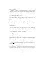
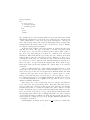
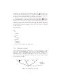
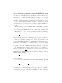
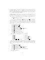
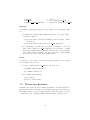
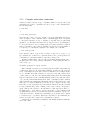

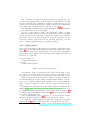
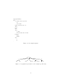
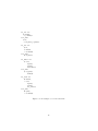
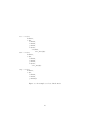
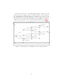
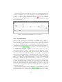
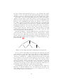
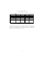


![[incr tsdb()]](http://vs1.manualzilla.com/store/data/005780303_1-7064634619abc733efac654e2a82e90d-150x150.png)