Download Which Step Do I Take First? Troubleshooting with Bayesian Models

Which Step Do I Take First? Troubleshooting with Bayesian Models
Annie Louis and Mirella Lapata
School of Informatics, University of Edinburgh
10 Crichton Street, Edinburgh EH8 9AB
{alouis,mlap}@inf.ed.ac.uk
Abstract
Online discussion forums and community
question-answering websites provide one of
the primary avenues for online users to share
information. In this paper, we propose text
mining techniques which aid users navigate
troubleshooting-oriented data such as questions asked on forums and their suggested solutions. We introduce Bayesian generative
models of the troubleshooting data and apply
them to two interrelated tasks: (a) predicting
the complexity of the solutions (e.g., plugging
a keyboard in the computer is easier compared
to installing a special driver) and (b) presenting them in a ranked order from least to most
complex. Experimental results show that our
models are on par with human performance
on these tasks, while outperforming baselines
based on solution length or readability.
1
Introduction
Online forums and discussion boards have created
novel ways for discovering, sharing, and distributing information. Users typically post their questions or problems and obtain possible solutions from
other users. Through this simple mechanism of
community-based question answering, it is possible
to find answers to personal, open-ended, or highly
specialized questions. However, navigating the information available in web-archived data can be
challenging given the lack of appropriate search and
browsing facilities.
Table 1 shows examples typical of the problems
and proposed solutions found in troubleshootingoriented online forums. The first problem concerns a
shaky monitor and has three solutions with increasing degrees of complexity. Solution (1) is probably
easiest to implement in terms of user time, effort,
and expertise; solution (3) is most complex (i.e., the
user should understand what signal timing is and
The screen is shaking.
1. Move all objects that emit a magnetic field, such as a
motor or transformer, away from the monitor.
2. Check if the specified voltage is applied.
3. Check if the signal timing of the computer system is
within the specification of the monitor.
“Illegal Operation has Occurred” error message is
displayed.
1. Software being used is not Microsoft-certified for your
version of Windows. Verify that the software is certified
by Microsoft for your version of Windows (see program
packaging for this information).
2. Configuration files are corrupt. If possible, save all data,
close all programs, and restart the computer.
Table 1: Example problems and solutions taken from online troubleshooting oriented forums.
then try to establish whether it is within the specification of the monitor), whereas solution (2) is somewhere in between. In most cases, the solutions are
not organized in any particular fashion, neither in
terms of content nor complexity.
In this paper, we present models to automatically
predict the complexity of troubleshooting solutions,
which we argue could improve user experience, and
potentially help solve the problem faster (e.g., by
prioritizing easier solutions). Automatically structuring solutions according to complexity could also
facilitate search through large archives of solutions
or serve as a summarization tool. From a linguistic perspective, learning how complexity is verbalized can be viewed as an instance of grounded language acquisition. Solutions direct users to carry
out certain actions (e.g., on their computers or devices) and complexity is an attribute of these actions. Information access systems incorporating a
notion of complexity would allow to take user intentions into account and how these translate into
natural language. Current summarization and information retrieval methods are agnostic of such types
of text semantics. Moreover, the models presented
here could be used for analyzing collaborative prob-
lem solving and its social networks. Characterizing
the content of discussion forums by their complexity
can provide additional cues for identifying user authority and if there is a need for expert intervention.
We begin by validating that the task is indeed
meaningful and that humans perceive varying degrees of complexity when reading troubleshooting
solutions. We also show experimentally that users
agree in their intuitions about the relative complexity of different solutions to the same problem. We
define “complexity” as an aggregate notion of the
time, expertise, and money required to implement
a solution. We next model the complexity prediction task, following a Bayesian approach. Specifically, we learn to assign complexity levels to solutions based on their linguistic makeup. We leverage
weak supervision in the form of lists of solutions (to
different problems) approximately ordered from low
to high complexity (see Table 1). We assume that
the data is generated from a fixed number of discrete complexity levels. Each level has a probability
distribution over the vocabulary and there is a canonical ordering between levels indicating their relative
complexity. During inference, we recover the vocabularies of the complexity levels and the ordering
of levels that explains the solutions and their attested
sequences in the training data.
We explore two Bayesian models differing in how
they learn an ordering among complexity levels. The
first model is local, it assigns an expected position
(in any list of solutions) to each complexity level
and orders the levels based on this expected position value. The second model is global, it defines
probabilities over permutations of complexity levels and directly uncovers a consensus ordering from
the training data. We evaluate our models on a solution ordering task, where the goal is to rank solutions from least to most complex. We show that
a supervised ranking approach using features based
on the predictions of our generative models is on par
with human performance on this task while outperforming competitive baselines based on length and
readability of the solution text.
2
Related work
There is a long tradition of research on decisiontheoretic troubleshooting where the aim is to find
a cost efficient repair strategy for a malfunctioning device (Heckerman et al., 1995). Typically, a
diagnostic procedure (i.e., a planner) is developed
that determines the next best troubleshooting step
by estimating the expected cost of repair for various
plans. Costs are specified by domain experts and are
usually defined in terms of time and/or money incurred by carrying out a particular repair action. Our
notion of complexity is conceptually similar to the
cost of an action, however we learn to predict complexity levels rather than calibrate them manually.
Also note that our troubleshooting task is not device
specific. Our models learn from troubleshootingoriented data without any restrictions on the problems being solved.
Previous work on web-based user support has
mostly focused on thread analysis. The idea is to
model the content structure of forum threads by analyzing the requests for information and suggested
solutions in the thread data (Wang et al., 2011; Kim
et al., 2010). Examples of such analysis include
identifying which earlier post(s) a given post responds to and in what manner (e.g., is it a question,
an answer or a confirmation). Other related work
(Lui and Baldwin, 2009) identifies user characteristics in such data, i.e., whether users express themselves clearly, whether they are technically knowledgeable, and so on. Although our work does not
address threaded discourse, we analyze the content
of troubleshooting data and show that it is possible
to predict the complexity levels for suggested solutions from surface lexical cues.
Our work bears some relation to language grounding, the problem of extracting representations of the
meaning of natural language tied to the physical
world. Mapping instructions to executable actions
is an instance of language grounding with applications to automated troubleshooting (Branavan et al.,
2009; Eisenstein et al., 2009), navigation (Vogel and
Jurafsky, 2010), and game-playing (Branavan et al.,
2011). In our work, there is no direct attempt to
model the environment or the troubleshooting steps.
Rather, we study the language of instructions and
how it correlates with the complexity of the implied
actions. Our results show that it possible to predict
complexity, while being agnostic about the semantics of the domain or the effect of the instructions in
the corresponding environment.
Our generative models are trained on existing
archives of problems with corresponding solutions
(approximately ordered from least to most complex)
3
Problem formulation
Our aim in this work is to learn models which can
automatically reorder solutions to a problem from
low to high complexity. Let G = (c1 , c2 , .. cN ) be
a collection of solutions to a specific problem. We
wish to output a list G0 = (c01 , c02 , .. c0N ), such that
D(c0j ) ≤ D(c0j+1 ), where D(x) refers to the complexity of solution x.
3.1
Corpus Collection
As training data we are given problem-solution sets
similar to the examples in Table 1 where the solutions are approximately ordered from low to high
complexity. A solution set Si is specific to problem Pi , and contains an ordered list of NPi solutions Si = (x1 , x2 , . . . , xNPi ) such that D(xj ) <
D(xj+1 ). We refer to the number of solutions related to a problem, NPi , as its solution set size.
For our experiments, we collected 300 problems1
and their solutions from multiple web sites including the computing support pages of Microsoft, Apple, HP, as well as amateur computer help websites
such as www.computerhope.com. The problems were mostly frequently asked questions (FAQs)
referring to malfunctioning personal computers and
smart phones. The solutions were provided by computer experts or experienced users in the absence
1
The corpus can be downloaded from http:
//www.homepages.inf.ed.ac.uk/alouis/
solutionComplexity.html.
Frequency
and learn to predict an ordering for new sets of solutions. This setup is related to previous studies
on information ordering where the aim is to learn
statistical patterns of document structure which can
be then used to order new sentences or paragraphs
in a coherent manner. Some approaches approximate the structure of a document via topic and entity
sequences using local dependencies such as conditional probabilities (Lapata, 2003; Barzilay and Lapata, 2008) or Hidden Markov Models (Barzilay and
Lee, 2004). More recently, global approaches which
directly model the permutations of topics in the document have been proposed (Chen et al., 2009b). Following this line of work, one of our models uses
the Generalized Mallows Model (Fligner and Verducci, 1986) in its generative process which allows
to model permutations of complexity levels in the
training data.
70
65
60
55
50
45
40
35
30
25
20
15
10
5
0
2
3
4
5
6
7
8
9
10 11 12 13 14 15 16
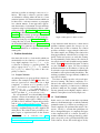
Solution set size
Figure 1: Histogram of solution set sizes
of any interaction with other users or their devices
and thus constitute a generic list of steps to try out.
We assume that in such a situation, the solution
providers are likely to suggest simpler solutions before other complex ones, leading to the solution lists
being approximately ordered from low to high complexity. In the next section, we verify this assumption experimentally. In this dataset, the solution set
size varies between 2 and 16 and the average number
is 4.61. Figure 1 illustrates the histogram of solution
set sizes found in our corpus. We only considered
problems which have no less than two solutions. All
words in the corpus were lemmatized and html links
and numbers were replaced with placeholders. The
resulting vocabulary was approximately 2,400 word
types (62,152 tokens).
Note that our dataset provides only weak supervision for learning. The relative complexity of solutions for the same problem is observed, however,
the relative complexity of solutions across different
problems is unknown. For example, a hardware issue may generally receive highly complex solutions
whereas a microphone issue mostly simple ones.
3.2
Task Validation
In this section, we detail an annotation experiment
where we asked human judges to rank the randomly
permuted contents of a solution set according to perceived complexity. We performed this study for two
reasons. Firstly, to ascertain that participants are
able to distinguish degrees of complexity and agree
on the complexity level of a solution. Secondly, to
examine whether the ordering produced by participants corresponds to the (gold-standard) FAQ order
of the solutions. If true, this would support our hy-
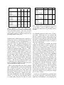
A
B
C
D
B
0.421
C
0.525
0.436
D
0.625
0.434
0.584
FAQ
0.465
0.252
0.303
0.402
Table 2: Correlation matrix for annotators (A–D) and
original FAQ order using Kendall’s τ (values are averages over 100 problem-solution sets).
pothesis that the solutions in our FAQ corpus are frequently presented according to complexity and that
this ordering is reasonable supervision for our models.
Method We randomly sampled 100 solution sets
(their sizes vary between 2 and 16) from the
FAQ corpus described in the previous section and
randomly permuted the contents of each set. Four
annotators, one an author of this paper, and three
graduate and undergraduate students in Computer
Science were asked to order the solutions in each
set from easy to most complex. An easier solution
was defined as one “which takes less time or effort
to carry out by a user”. The annotators saw a list of
solutions for the same problem on a web interface
and assigned a rank to each solution to create an order. No ties were allowed and a complete ordering
was required to keep the annotation simple. The annotators were fluent English speakers and had some
knowledge of computer hardware and software. We
refrained from including novice users in our study as
they are likely to have very different personal preferences resulting in more divergent rankings.
Results We measured inter-annotator agreement
using Kendall’s τ , a metric of rank correlation which
has been reliably used in information ordering evaluations (Lapata, 2006; Bollegala et al., 2006; Madnani et al., 2007). τ ranges between −1 and +1,
where +1 indicates equivalent rankings, −1 completely reverse rankings, and 0 independent rankings. Table 2 shows the pairwise inter-annotator
agreement as well as the agreement between each
annotator and the original FAQ order. The table
shows fair agreement between the annotators confirming that this is a reasonable task for humans to
do. As can be seen, there are some individual differences, with the inter-annotator agreement varying
from 0.421 (for A,B) to 0.625 (for A,D).
The last column in Table 2 reports the agreement
between our annotator rankings and the original ordering of solutions in the FAQ data. Although there
is fair agreement with the FAQ providing support for
its use as a gold-standard, the overall τ values are
lower compared to inter-annotator agreement. This
implies that the ordering may not be strictly increasing in complexity in our dataset and that our models
should allow for some flexibility during learning.
Several reasons contributed to disagreements between annotators and with the FAQ ordering, such
as the users’ expertise, personal preferences, or the
nature of the solutions. For instance, annotators disagreed when multiple solutions were of similar complexity. For the first example in Table 1, all annotators agreed perfectly and also matched the FAQ
order. For the second example, the annotators disagreed with each other and the FAQ.
4
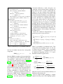
Generative Models
In the following we introduce two Bayesian topic
models for the complexity prediction (and ranking) task. In these models, complexity is captured
through a discrete set D of L levels and a total ordering between the levels reflects their relative complexity. In other words, D = (d1 , d2 , ...dL ), where
d1 is easiest level and D(dm ) < D(dm+1 ) . Each
complexity level is parametrized by a unigram language model which captures words likely to occur
in solutions with that level.
Our two models are broadly similar. Their generative process assigns a complexity level from D
to each solution such that it explains the words
in the solution and also the ordering of solutions within each solution set. Words are generated for each solution by mixing problem-specific
words with solution-specific (and hence complexityrelated) ones. Also, each problem has its own distribution over complexity levels which allows for some
problems to have more complex solutions on average, some a mix of high and low complexity solutions, or otherwise predominantly easier solutions.
The main difference between the two models is
in the way they capture the ordering between levels.
Our first model infers a distribution for each level
over the positions at which a solution with that complexity can occur and uses this distribution to order
the levels. Levels which on average occur at greater
positions have higher complexity. The second model
defines probabilities over orderings of levels in the
Corpus level
For each complexity level dm , 1 ≤ m ≤ L,
- Draw a complexity vocabulary distribution
φm ∼ Dirichlet(α)
- Draw a distribution over positions
γm ∼ Dirichlet(ρ)
- Draw a distribution ψ for the proportion of complexityversus problem-specific vocabulary ∼ Beta(δ0 , δ1 )
Solution set level
For each solution set Qi in the corpus, 1 ≤ i ≤ N ,
- Draw a distribution over the complexity levels
θi ∼ Dirichlet(β)
- Draw a problem-specific vocabulary distribution
λi ∼ Dirichlet(ω)
Individual solution level
For each solution xij in Qi , 1 ≤ j ≤ NPi ,
- Draw a complexity level assignment,
zij ∼ Multinomial(θi )
- Draw a position depending on the level assigned,
rij ∼ Multinomial(γzij )
Word level
For each word wijk in solution xij ,
- Draw a switch value to indicate if the word is
problem- or complexity-specific, sijk ∼ Binomial(ψ)
- If sijk = 0, draw wijk ∼ Multinomial(φzij )
- If sijk = 1, draw wijk ∼ Multinomial(λi )
Figure 2: Generative process for the Position Model
generative process itself. The inference process of
this model allows to directly uncover a canonical ordering of the levels which explains the training data.
4.1
Expected Position model
This model infers the vocabulary associated with a
complexity level and a distribution over the numerical positions in a solution set where such a complexity level is likely to occur. After inference, the
model uses the position distribution to compute the
expected position of each complexity level. The levels are ordered from low to high expected position
and taken as the order of increasing complexity.
The generative process for our model is described
in Figure 2. A first phase generates the latent variables which are drawn once for the entire corpus.
Then, variables are drawn for a solution set, next for
each solution in the set, and finally for the words in
the solutions. The number of complexity levels L
is a parameter in the model, while the vocabulary
size V is fixed. For each complexity level dm , we
draw one multinomial distribution φ over the vocabulary V , and another multinomial γ over the possible positions. These two distributions are drawn
from symmetric Dirichlet priors with hyperparameters α and ρ. Solutions will not only contain words
relating to their complexity but also to the problem or malfunctioning component at hand. We assume these words play a minor role in determining
complexity and thus draw a binomial distribution ψ
that balances the amount of problem-specific versus complexity-specific vocabulary. This distribution has a Beta prior with hyperparameters δ0 and δ1 .
For each solution set, we draw a distribution over
the complexity levels θ from another Dirichlet prior
with concentration β. This distribution allows each
problem to take a different preference and mix of
complexity levels for its solutions. Another multinomial λ over the vocabulary is drawn for the problemspecific content of each solution set. λ is given a
symmetric Dirichlet prior with concentration ω.
For each individual solution in a set, we draw a
complexity level z from θ, i.e., the complexity level
proportions for that problem. A position for the solution is then drawn from the position distribution
for that level, i.e., γz . The words in the solution are
generated by first drawing a switch value for each
word indicating if the word came from the problem’s
technical or complexity vocabulary. Accordingly,
the word is drawn from λ or φz .
During inference, we are interested in the posterior of the model given the FAQ training data. Based
on the conditional independencies of the model, the
posterior is proportional to:
P (ψ|δ0 , δ1 ) ×
L
Q
[P (φm |α)] ×
m=1
N
Q
×
N
Q
×
i=1
Pi
N N
Q
Q
×
i=1 j=1
Pi |xij |
N N
Q
Q
Q
[P (θi |β)] ×
L
Q
[P (γm |ρ)]
m=1
[P (λi |ω)]
i=1
[P (zij |θi )P (rij |γzij )]
[P (sijk |ψ)P (wijk |sijk , φzij , λi )]
i=1 j=1 k=1
where L is the number of complexity levels, N the
number of problems in the training corpus, NPi the
size of solution set for problem Pi , and |xij | the
number of words in solution xij .
The use of conjugate priors for the multinomial
and binomial distributions allows us to integrate out
the ψ, φ, γ, λ and θ distributions. The simplified
posterior is proportional to:
L
Q
Γ(Rim +βm )
m=1
!
L
i=1 Γ P Rm +βm
i
N
Q
×
m=1
1
Q
×
Γ(T u +δ
u=0
1
P
Γ
u)
T u +δu
u=0
×
G
Q
Γ(Qrm +ρr )
r=1
!
G
m=1 Γ P Qr +ρr
m
L
Q
r=1
V
Q
0 (v)+α
Γ(Tm
v)
v=1
!
V
m=1 Γ P T 0 (v)+αv
m
L
Q
v=1
V
Q
Γ(Ti1 (v)+ωv )
v=1
!
×
V
i=1 Γ P T 1 (v)+ωv
i
N
Q
tions for each complexity level dm over the vocabulary φm and positions γm . We compute the expected
position Ep of dm as:
v=1
where Rim is the number of times level m is assigned to a solution in problem i. Qrm is the number of times a solution with position r is given complexity m over the full corpus. Positions are integer
values between 1 and G. T 0 and T 1 count the number of switch assignments of value 0 (complexityrelated word) and 1 (technical word) respectively in
0 (v) is a refined count of the number
the corpus. Tm
of times word type v is assigned switch value 0 in a
solution of complexity m. Ti1 (v) counts the number
of times switch value 1 is given to word type v in a
solution set for problem i.
We sample from this posterior using a collapsed
Gibbs sampling algorithm. The sampling sequence
starts with a random initialization to the hidden variables. During each iteration, the sampler chooses
a complexity level for each solution based on the
current assignments to all other variables. Then the
switch values for the words in each solution are sampled one by one. The hyperparameters are tuned using grid search on development data. The language
model concentrations α, ρ and ω are given values
less than 1 to obtain sparse distributions. The prior
on θ, the topic proportions, is chosen to be greater
than 1 to encourage different complexity levels to be
used within the same problem rather than assigning
all solutions to the same one or two levels. Similarly,
δ0 and δ1 are > 1. We run 5,000 sampling iterations
and use the last sample as a draw from the posterior.
Using these assignments, we also compute an estimate for the parameters φm , λi and γm . For example, the probability of a word v in φm is computed
0
m (v)+αv
as P T(T
.
0
v m (v)+αv )
After inference, we obtain probability distribu-
Ep (dm ) =
G
X
pos ∗ γm (pos)
(1)
pos=1
where pos indicates position values. Then, we rank
the levels in increasing order of Ep .
4.2
Permutations-based model
In our second model we incorporate the ordering
of complexity levels in the generative process itself.
This is achieved by using the Generalized Mallows
Model (GMM; Fligner and Verducci (1986)) within
our hierarchical generative process. The GMM is
a probabilistic model over permutations of items
and is frequently used to learn a consensus ordering
given a set of different rankings. It assumes there is
an underlying canonical order of items and concentrates probability mass on those permutations that
differ from the canonical order by a small amount,
while assigning lesser probability to very divergent
permutations. Probabilistic inference in this model
uncovers the canonical ordering.
The standard Mallows model (Mallows, 1957)
has two parameters, a canonical ordering σ and a
dispersion penalty ρ > 0. The probability of an observed ordering π is defined as:
P (π|ρ, σ) =
e−ρd(π,σ)
,
ξ(ρ)
where d(π, σ) is a distance measure such as
Kendall’s τ , between the canonical ordering σ and
an observed ordering π. The GMM decomposes
d(π, σ) in a way that captures item-specific distance. This is done by computing an inversion vector representation of d(π, σ). A permutation π of n
items can be equivalently represented by a vector of
inversion counts v of length n − 1, where each component vi equals the number of items j > i that occur before item i in π. The dimension of v is n − 1
since there can be no items greater than the highest value element. A unique inversion vector can be
computed for any permutation and vice versa, and
the sum of the inversion vector elements is equal
to d(π, σ). Each vi is also given a separate dispersion penalty ρi . Then, the GMM is defined as:
Y
GMM(v|ρ) ∝
e−ρi vi
(2)
i
Corpus level
For each complexity level dm , 1 ≤ m ≤ L,
- Draw a complexity vocabulary distribution
φm ∼ Dirichlet(α)
- Draw the L − 1 dispersion parameters
ρr ∼ GMM0 (µ0 ,v0r )
- Draw a distribution ψ for the proportion of complexityversus problem-specific vocabulary ∼ Beta(δ0 , δ1 )
Solution set level
For each solution set Qi in the corpus, 1 ≤ i ≤ N ,
- Draw a distribution over the complexity levels
θi ∼ Dirichlet(β)
- Draw a problem-specific vocabulary distribution
λi ∼ Dirichlet(ω)
- Draw a bag of NPi levels for the solution set
bi ∼ Multinomial(θi )
- Draw an inversion vector vi
vi ∼ GMM(ρ)
- Compute permutation πi of levels using vi
- Compute level assignments zi using πi and bi .
Assign level zij to xij for 1 ≤ j ≤ NPi .
Word level
For each word wijk in solution xij ,
- Draw a switch value to indicate if the word is
problem- or complexity-specific, sijk ∼ Binomial(ψ)
- If sijk = 0, draw wijk ∼ Multinomial(φzij )
- If sijk = 1, draw wijk ∼ Multinomial(λi )
a binomial distribution, ψ (with a beta prior) over
complexity- versus problem-specific vocabulary. At
the solution set level, we draw a multinomial distribution λ over the vocabulary and a multinomial
distribution θ for the proportion of L levels for this
problem. Both these distributions have Dirichlet priors. Next, we generate an ordering for the complexity levels. We draw NPi complexity levels from θ,
one for each solution in the set. Let b denote this
bag of levels (e.g., b = (1, 1, 2, 3, 4, 4, 4) assuming
4 complexity levels and 7 solutions for a particular
problem). We also draw an inversion vector v from
the GMM distribution which advantageously allows
for small differences from the canonical order. The
z assignments are deterministically computed by ordering the elements of b according to the permutation defined by v.
Given the conditional independencies of our
model, the posterior is proportional to:
Figure 3: Generative process for Permutation Model.
where L is the number of complexity levels, N the
total problems in the training corpus, NPi the size
of solution set for problem Pi , and |xij | the number
of words in solution xij . A simplified posterior can
be obtained by integrating out the ψ, φ, λ, and θ
distributions which is proportional to:
And can be further factorized into item-specific
components:
GMMi (vi |ρi ) ∝ e−ρi vi
(3)
Since the GMM is a member of the exponential family, a conjugate prior can be defined for each dispersion parameter ρi which allows for efficient inference. We refer the interested reader to Chen et al.
(2009a) for details on the prior distribution and normalization factor for the GMM distribution.
Figure 3 formalizes the generative story of our
own model which uses the GMM as a component.
We assume the canonical order is the strictly increasing (1, 2, .., L) order. For each complexity level dm ,
we draw a distribution φ over the vocabulary. We
also draw L − 1 dispersion parameters from the conjugate prior GMM0 density. Hyperparameters for
this prior are set in a similar fashion to Chen et
al. (2009a). As in the position model, we draw
L
Q
[P (φm |α)] ×
m=1
N
Q
×
×
L−1
Q
[P (ρr |µ0 , v0r )] × P (ψ|δ0 , δ1 )
r=1
[P (θi |β)
i=1
Pi |xij |
N N
Q
Q
Q
× P (λi |ω) × P (vi |ρ) × P (bi |θi )]
[P (sijk |ψ)P (wijk |sijk , φzij , λi )]
i=1 j=1 k=1
N
Q
L
Q
Γ(Rim +βm )
!
m=1
L
P
i=1 Γ
m=1
×
N L−1
Q
Q
Rim +βm
×
L−1
Q
1
Q
GMMr (vir |ρr ) ×
i=1 r=1
v=1
×
Γ(T u +δu )
T u +δu
u=0
1
P
Γ
V
Q
0 (v)+α
Γ(Tm
v)
v=1
!
×
V
m=1 Γ P T 0 (v)+αv
m
L
Q
GMM0 (ρr |µ0 , v0r )
r=1
N
Q
u=0
V
Q
Γ(Ti1 (v)+ωv )
!
v=1
V
P
i=1 Γ
v=1
Ti1 (v)+ωv
where the R and T counts are defined similarly as in
the Expected Position model.
We use collapsed Gibbs sampling to compute
samples from this posterior. The sampling sequence
Level 1
free, space, hard, drive, sure, range, make, least, more, operate, than, point, less, cause, slowly, access, may, problem
Level 2
use, can, media, try, center, signal, network, make, file, sure,
when, case, with, change, this, setting, type, remove
Level 19
system, file, this, restore, do, can, then, use, hard, issue,
NUM, will, disk, start, step, above, run, cleanup, drive, xp
Level 20
registry, restore, may, virus, use, bio, setting, scanreg, first,
ensure, can, page, about, find, install, additional, we, utility
Table 3: Most likely words assigned to varying complexity levels by the permutations-based model.
randomly initializes the hidden variables. For a chosen solution set Si , the sampler draws NPi levels
(bi ), one at a time conditioned on the assignments
to all other hidden variables of the model. Then
the inversion vector vi is created by sampling each
vij in turn. At this point, the complexity level assignments zi can be done deterministically given bi
and vi . Then the words in each solution set are
sampled one at a time. For the dispersion parameters, ρ, the normalization constant of the conjugate
prior is not known. We sample from the unnormalized GMM0 distribution using slice sampling.
Other hyperparameters of the model are tuned using development data. The language model Dirichlet
concentrations (α, ω) are chosen to encourage sparsity and β > 1 as in the position model. We run
the Gibbs sampler for 5,000 iterations; the dispersion parameters are resampled every 10 iterations.
The last sample is used as a draw from the posterior.
4.3
Model Output
In this section we present examples of the complexity assignments created by our models. Table 3
shows the output of the permutations-based model
with 20 levels. Each row contains the highest probability words in a single level (from the distribution φm ). For the sake of brevity, we only show the
two least and most complex levels. In general, we
observe more specialized, technical terms in higher
levels (e.g., restore, scanreg, registry) which one
would expect to correlate with complex solutions.
Also note that higher levels contain uncertainty denoting words (e.g., can, find, may) which again are
indicative of increasing complexity.
Using these complexity vocabularies, our models
1.0
1.0
1.0
5.7
5.5
5.1
10.0
10.0
9.9
Low complexity
Cable(s) of new external device are loose or power cables are unplugged. Ensure that all cables are properly
and securely connected and that pins in the cable or
connector are not bent down.
Make sure your computer has at least 50MB of free
hard drive space. If your computer has less than
50MB free, it may cause the computer to operate more
slowly.
If the iPhone is in a protective case, remove it from
the case. If there is a protective film on the display,
remove the film.
Medium complexity
Choose a lower video setting for your imported video.
The file property is set to read-only. To work around
this issue, remove the read-only property. For more
information about file properties, see View the properties for a file.
The system is trying to start from a media device that
is not bootable. Remove the media device from the
drive.
High complexity
If you are getting stopped at the CD-KEY or Serial
Number verification, verify you are entering your correct number. If you lost your number or key or it does
not work, you will need to contact the developer of the
program. Computer Hope will not provide any users
with an alternate identification number.
The network controller is defective. Contact an authorized service provider.
Network controller interrupt is shared with an expansion board. Under the Computer Setup Advanced
menu, change the resource settings for the board.
Table 4: Example solutions with low, medium and high
expected complexity values (position-based model with
10 complexity levels). The solutions come from various
problem-solution sets in the training corpus. Expected
complexity values are shown in the first column.
can compute the expected complexity for
P any solution text, x. This value is given by [ L
m=1 m ∗
p(m|x)]. We estimate the second term, p(m|x),
using a) the complexity level language models φm
and b) a prior over levels given by the overall frequency of different levels on the training data. Table 4 presents examples of solution texts from our
training data and their expected complexity under
the position-model. We find that the model is able to
distinguish intuitively complex solutions from simpler ones. Aside from measuring expected complexity in absolute terms, our models can also also order solutions in terms of relative complexity (see
the evaluation in Section 5) and assign a complexity value to a problem as a whole.
Low Complexity Problems
- Computer appears locked up and will not turn off when the
power button is pressed.
- A USB device, headphone, or microphone is not recognized
by the computer.
- Computer will not respond to USB keyboard or mouse.
High Complexity Problems
- Game software and driver issues.
- Incorrect, missing or stale visible networks.
- I get an error message that says that there is not enough disk
space to publish the movie. What can I do?
- Power LED flashes Red four times, once every second, followed by two second pause, and computer beeps four times.
Table 5: Least and most complex problems based on the
expected complexity of their solution set. Problems are
shown with complexity 1–3 (top) and 8–9 (bottom) using
the position-based model.
As mentioned earlier, our models only observe the
relative ordering of solutions to individual problems;
the relative complexity of two solutions from different problems is not known. Nevertheless, the models
are able to rate solutions on a global scale while accommodating problem-specific ordering sequences.
Specifically, we can compute the expected complexity of the solution set for problemPi, using the inL
ferred distribution over levels θi :
m=1 m × θim .
Table 5 shows the complexity of different problems
as predicted by the position model (with 10 levels).
As can be seen, easy problems are associated with
accessory components (e.g., mouse or keyboard),
whereas complex problems are related to core hardware and operating system errors.
5
Evaluation Experiments
In the previous section, we showed how our models can assign an expected complexity value to a solution text or an entire problem. Now, we present
evaluations based on model ability to order solutions
according to relative complexity.
5.1
Solution Ordering Task
We evaluated our models by presenting them with
a randomly permuted set of solutions to a problem
and examining the accuracy with which they reorder
them from least to most complex. At first instance,
it would be relatively straightforward to search for
the sequence of solutions which has high likelihood
under the models. Unfortunately, there are two problems with this approach. Firstly, the likelihood under our models is intractable to compute, so we
would need to adopt a simpler and less precise approximation (such as the Hidden Markov Model discussed below). Secondly, when the solution set size
is large, we cannot enumerate all permutations and
need to adopt an approximate search procedure.
We opted for a discriminative ranking approach
instead which uses the generative models to compute
a rich set of features. This choice allows us to simultaneously obtain features tapping on to different aspects learned by the models and to use well-defined
objective functions. Below, we briefly describe the
features based on our generative models. We also
present additional features used to create baselines
for system comparison.
Likelihood We created a Hidden Markov Model
based on the sample from the posterior of our models (for a similar HMM approximation of a Bayesian
model see Elsner et al. (2007)). For our model, the
HMM has L states, and each state sm corresponds
to a complexity level dm . We used the complexity language models φm estimated from the posterior as the emission probability distribution for the
corresponding states. The transition probabilities of
the HMM were computed based on the complexity
level assignments for the training solution sequences
in our posterior sample. The probability of transitioning to state sj from state si , p(sj |si ), is the conc(d ,d )
ditional probability p(dj |di ) computed as c(di i )j ,
where c(di , dj ) is the number of times the complexity level dj is assigned to a solution immediately following a solution which was given complexity di .
c(di ) is the number of times complexity level di is
assigned overall in the training corpus. We perform
Laplace smoothing to avoid zero probability transitions between states:
p(sj |si ) =
c(di , dj ) + 1
c(di ) + L
(4)
This HMM formulation allows us to use efficient dynamic programming to compute the likelihood of a
sequence of solutions.
Given a solution set, we compute an ordering as
follows. We enumerate all orderings for sets with
size less than 6, and select the sequence with the
highest likelihood. For larger sizes, we use a simulated annealing search procedure which swaps two
adjacent solutions in each step. The temperature was
set to 50 initially and gradually reduced to 1. These
values were set using minimal tuning on the development data. After estimating the most likely sequence for a solution set, we used the predicted rank
of each solution as a feature in our discriminative
model.
Expected Complexity As mentioned earlier, we
computed
the expected complexity of a solution x
P
as [ L
m=1 m ∗ p(m|x)], where the second term was
estimated using a complexity level specific language
model φm and a uniform prior over levels on the
test set. As additional features, we used the solution’s perplexity under each φm , and under each of
the technical topics λi , and also the most likely level
for the text arg maxm p(m|x). Finally, we included
features for each word in the training data. The feature value is the word’s expected level multiplied by
the probability of the word in the solution text.
Length We also investigated whether solution
length is a predictor of complexity (e.g., simple solutions may vary in length and amount of detail from
complex ones). We devised three features based on
the number of sentences (within a solution), words,
and average sentence length.
Syntax/Semantics Another related class of features estimates solution complexity based on sentence structure and meaning. We obtained eight
syntactic features based on the number of nouns,
verbs, adjectives and adverbs, prepositions, pronouns, wh-adverbs, modals, and punctuation. Other
features compute the average and maximum depth
of constituent parse trees. The part-of-speech tags
and parse trees were obtained using the Stanford
CoreNLP toolkit (Manning et al., 2014). In addition, we computed 10 semantic features using WordNet (Miller, 1995). They are the average number of senses for each category (noun, verb, adjective/adverb), and the maximum number of senses for
the same three classes. We also include the average and maximum lengths of the path to the root of
the hypernym tree for nouns and verbs. This class
of features roughly approximates the indicators typically used in predicting text readability (Schwarm
and Ostendorf, 2005; McNamara et al., 2014).
5.2
Experimental Setup
We performed 10-fold cross-validation. We trained
the ranking model on 240 problem-solution sets;
30 sets were reserved for development and 30 for
testing (in each fold). The most frequent 20 words in
each training set were filtered as stopwords. The development data was used to tune the parameters and
hyperparameters of the models and the number of
complexity levels. We experimented with ranges [5–
20] and found that the best number of levels was 10
for the position model and 20 for the permutationbased model, respectively. For the expected position model, positions were normalized before training. Let solution xir denote the rth solution in the
solution set for problem Pi , where 1 ≤ r ≤ NPi .
We normalize r to a value between 0 and 1 using
. Then the [0–1]
a min-max method: r0 = Nr−1
Pi −1
range is divided into k bins. The identity of the bin
containing r0 is taken as the normalized position, r.
We tuned k experimentally during development and
found that k = 3 performed best.
For our ordering experiments we used Joachims’
(2006) SVMRank package for training and testing.
During training, the classifier learns to minimize the
number of swapped pairs of solutions over the training data. We used a linear kernel and the regularization parameter was tuned using grid search on the
development data of each fold. We evaluate how
well the model’s output agrees with gold-standard
ordering using Kendall’s τ .
5.3
Results
Table 6 summarizes our results (average Kendall’s τ
across folds). We present the results of the discriminative ranker when using a single feature class
based on likelihood and expected complexity (Position, Permutation), length, and syntactico-semantic
features (SynSem), and their combinations (denoted
via +). We also report the performance of a baseline which computes a random permutation for each
solution set (Random; results are averaged over five
runs). We show results for all solution sets (All) and
broken down into different set sizes (e.g., 2–3, 4–5).
As can be seen, the expected position model obtains an overall τ of 0.30 and the permutation model
of 0.26. These values lie in the range of human
annotator agreement with the FAQ order (see Section 3.2). In addition, we find that the models
perform consistently across solution set sizes, with
even higher correlations on longer sequences where
our methods are likely to be more useful. Position and Permutation outperform Random rankings
and a model based solely on Length features. The
Model
2–3
(133)
Random
-0.002
Length
-0.052
SynSem
0.167
Length+SynSem
0.122
Position
0.288
+Length
0.283
+SynSem
0.343
+SynSem+Length 0.348
Permutation
0.253
+Length
0.213
+SynSem
0.268
+SynSem+Length 0.253
Solution set sizes
4–5
>5
All
(81) (86) (300)
0.027 -0.006 0.004
-0.066 -0.028 -0.002
0.109 0.149 0.146
0.109 0.158 0.129
0.242 0.381 0.302
0.251 0.363 0.297
0.263 0.367 0.328
0.263 0.368 0.331
0.206 0.341 0.265
0.229 0.356 0.258
0.263 0.353 0.291
0.254 0.354 0.282
Table 6: Kendall’s τ values on the solution reordering task using 10-fold cross-validation and SVM ranking
models with different features. The results are broken
down by solution set size (the number of sets per size is
shown within parentheses). Boldface indicates the best
performing model for each set size.
SynSem features which measure the complexity of
writing in the text are somewhat better but still inferior compared to Position and Permutation. Using a paired Wilcoxon signed-rank test, we compared the τ values obtained by the different models. The Position and Permutation performed significantly better (p < 0.05) compared to Random,
Length and SynSem baselines. However, τ differences between Position and Permutation are not statistically significant. With regard to feature combinations, we observe that both models yield better performance when combined with Length or
SynSem. The Position model improves with the
addition of both Length and SynSem, whereas the
Permutation model combines best with SynSem
features. The Position+SynSem+Length model
is significantly better than Permutation (p < 0.05)
but not Permutation+SynSem+Length or Position
alone (again under the Wilcoxon test).
These results suggest that the solution ordering
task is challenging with several factors influencing
how a solution is perceived: the words used and
their meaning, the writing style of the solution, and
the amount of detail present in it. Our data comes
from the FAQs produced by computer and operating system manufacturers and other well-managed
websites. As a result, the text in the FAQ solutions
is of high quality. However, the same is not true
Model
Random
Length
SynSem
SynSem+Length
Position
+Length
+SynSem
+SynSem+Length
Permutation
+Length
+synsem
+SynSem+Length
Rank 1
15.3
18.1
19.8
20.6
31.0
36.2
34.4
36.2
28.4
30.1
32.7
32.7
Rank n
14.6
16.3
19.8
25.0
37.0
36.2
35.3
35.3
37.0
37.0
37.0
37.9
Both
3.4
6.8
4.3
5.1
13.7
18.9
16.3
17.2
12.0
15.5
13.7
13.7
Table 7: Model accuracy at predicting the easiest solution
correctly (Rank 1), the most difficult one (Rank n), or
both. Bold face indicates the best performing model for
each rank.
for community-generated solution texts on discussion forums. In the latter case, we conjecture that
the style of writing is likely to play a bigger role in
how users perceive complexity. We thus expect that
the benefit of adding Length and SynSem features
will become stronger when we apply our models to
texts from online forums.
We also computed how accurately the models
identify the least and most complex solutions. For
solution sets of size 5 and above (so that the task is
non-trivial) we computed the number of times the
rank one solution given by the models was also the
easiest according to the FAQ gold-standard. Likewise, we also computed how often the models correctly predict the most complex solution. With Random rankings, the easiest and most difficult solutions are predicted correctly 15% of the time. Getting both correct for a single problem happens only
3% of the time. The Position+Length model overall
performs best, identifying the easiest and most difficult solution 36% of the time. Both types of solution
are identified correctly 18% of the time. Interestingly, the generative models are better at predicting
the most difficult solution (35–37%) compared to
the easiest one (28–36%). One reason for this could
be that there are multiple easy solutions to try out
but the most difficult one is probably more unique
and so easier to identify.
Overall, we observe that the two generative models perform comparably, with Position having a
slight lead over Permutation. A key difference be-
tween the models is that during training Permutation
observes the full ordering of solutions while Position observes solutions coming from a few normalized position bins. Also note that in the Permutation model, multiple solutions with the same complexity level are grouped together in a solution set.
This property of the model is advantageous for ordering as solutions with similar complexity should
be placed adjacent to each other. At the same time, if
levels 1 and 2 are flipped in the permutation sampled
from the GMM, then any solution with complexity
level 1 will be ordered after the solution with complexity 2. The Position model on the other hand,
contains no special facility for grouping solutions
with the same complexity. In sum, Position can
more flexibly assign complexity levels to individual
solutions.
6
Conclusion
This work contains a first proposal to organize and
navigate crowd-generated troubleshooting data according to the complexity of the troubleshooting action. We showed that users perceive and agree on the
complexity of alternative suggestions, and presented
Bayesian generative models of the troubleshooting
data which can sort solutions by complexity with a
performance close to human agreement on the task.
Our results suggest that search and summarization tools for troubleshooting forum archives can be
greatly improved by automatically predicting and
using the complexity of the posted solutions. It
should also be possible to build broad coverage automated troubleshooting systems by bootstrapping
from conversations in discussion forums. In the future, we plan to deploy our models in several tasks
such as user authority prediction, expert intervention, and thread analysis. Furthermore, we aim to
specialize our models to include category-specific
complexity levels and also explore options for personalizing rankings for individual users based on
their knowledge of a topic and the history of their
troubleshooting actions.
Acknowledgements
We would like to thank the editor and the anonymous reviewers for their valuable feedback on an
earlier draft of this paper. We are also thankful to
members of the Probabilistic Models of Language
reading group at the University of Edinburgh for
their many suggestions and helpful discussions. The
first author was supported by a Newton International
Fellowship (NF120479) from the Royal Society and
the British Academy.
References
R. Barzilay and M. Lapata. 2008. Modeling local coherence: An entity-based approach. Computational Linguistics, 34(1):1–34.
R. Barzilay and L. Lee. 2004. Catching the drift: Probabilistic content models, with applications to generation
and summarization. In Proceedings of NAACL-HLT,
pages 113–120.
D. Bollegala, N. Okazaki, and M. Ishizuka. 2006.
A bottom-up approach to sentence ordering for
multi-document summarization. In Proceedings of
COLING-ACL, pages 385–392.
S. R. K. Branavan, H. Chen, L. S. Zettlemoyer, and
R. Barzilay. 2009. Reinforcement learning for mapping instructions to actions. In Proceedings of ACLIJCNLP, pages 82–90.
S. R. K. Branavan, D. Silver, and R. Barzilay. 2011.
Learning to win by reading manuals in a Monte-Carlo
framework. In Proceedings of ACL-HLT, pages 268–
277.
H. Chen, S. R. K. Branavan, R. Barzilay, and D. R.
Karger. 2009a. Content modeling using latent permutations. Journal of Artificial Intelligence Research,
36(1):129–163.
H. Chen, S.R.K. Branavan, R. Barzilay, and D.R. Karger.
2009b. Global models of document structure using
latent permutations. In Proceedings of NAACL-HLT,
pages 371–379.
J. Eisenstein, J. Clarke, D. Goldwasser, and D. Roth.
2009. Reading to learn: Constructing features from
semantic abstracts. In Proceedings of EMNLP, pages
958–967.
M. Elsner, J. Austerweil, and E. Charniak. 2007. A unified local and global model for discourse coherence.
In Proceedings of NAACL-HLT, pages 436–443.
M. A. Fligner and J. S. Verducci. 1986. Distance-based
ranking models. Journal of the Royal Statistical Society, Series B, pages 359–369.
D. Heckerman, J. S. Breese, and K. Rommelse. 1995.
Decision-theoretic troubleshooting. Communications
of the ACM, 38(3):49–57.
T. Joachims. 2006. Training linear SVMs in linear time.
In Proceedings of KDD, pages 217–226.
S. Kim, L. Cavedon, and T. Baldwin. 2010. Classifying
dialogue acts in one-on-one live chats. In Proceedings
of EMNLP, pages 862–871.
M. Lapata. 2003. Probabilistic text structuring: Experiments with sentence ordering. In Proceedings of ACL,
pages 545–552.
M. Lapata. 2006. Automatic evaluation of information
ordering. Computational Linguistics, 32(4):471–484.
M. Lui and T. Baldwin. 2009. Classifying user forum
participants: Separating the gurus from the hacks, and
other tales of the internet. In Proceedings of the 2010
Australasian Language Technology Workshop, pages
49–57.
N. Madnani, R. Passonneau, N. Ayan, J. Conroy, B. Dorr,
J. Klavans, D. O’Leary, and J. Schlesinger. 2007.
Measuring variability in sentence ordering for news
summarization. In Proceedings of the Eleventh European Workshop on Natural Language Generation.
C. L. Mallows. 1957. Non-null ranking models. i.
Biometrika, 44(1/2):pp. 114–130.
C. D. Manning, M. Surdeanu, J. Bauer, J. Finkel, S. J.
Bethard, and D. McClosky. 2014. The Stanford
CoreNLP natural language processing toolkit. In Proceedings of ACL: System Demonstrations, pages 55–
60.
D. S. McNamara, A. C. Graesser, P. M. McCarthy, and
Z. Cai. 2014. Automated evaluation of text and discourse with Coh-Metrix. Cambridge University Press.
G. A. Miller. 1995. WordNet: a lexical database for
English. Communication of the ACM, 38(11):39–41.
S. Schwarm and M. Ostendorf. 2005. Reading level assessment using support vector machines and statistical
language models. In Proceedings of ACL, pages 523–
530.
A. Vogel and D. Jurafsky. 2010. Learning to follow
navigational directions. In Proceedings of ACL, pages
806–814.
L. Wang, M. Lui, S. Kim, J. Nivre, and T. Baldwin.
2011. Predicting thread discourse structure over technical web forums. In Proceedings of EMNLP, pages
13–25.