Download CLab# 1.0: A Configuration Support Tool Based on Constraint

CLab# 1.0:
A Configuration Support Tool Based on Constraint
Programming and Binary Decision Diagrams
Torbjørn Meistad, Yngve Raudberget and Geir-Tore Lindsve
September 2006
IT University of Copenhagen
Rued Langgaards Vej 7
DK-2300 Copenhagen S
Copyright c 2006 Torbjørn Meistad, Yngve Raudberget and Geir-Tore Lindsve
Abstract
In our every day lives we are surrounded by restrictions and alternatives
and the notion of some space of parameters and attributes that we need to consider. Many of these scenarios can be described as configuration problems, and
solved using configuration solvers. The basis for such solvers can be constraint
programming or binary decision diagrams.
This thesis presents design, application, implementation, and evaluation
of CLab# as a software for fast backtrack-free interactive product configuration. It can use either constraint programming (CSP) or binary decision diagrams (BDDs) by encoding the configuration problem in binary, for solving
user-defined configuration problems, seamlessly switching between the two
approaches.
Using either approach lets end users such as students and researchers in the
field of AI and related sciences compare the performance of online search using
constraint programming algorithms against the performance of offline/online
reasoning using binary decision diagrams. CLab# utilizes the BuDDy BDD
package for handling BDDs and CaSPer for handling CSPs. CLab# works side
by side with these packages, without being strictly tied to either.
To ease the use of the library, a graphical user interface application has
been developed which provides both an editor for configuration files and an
interactive configurator interface for solving configuration problems.
A series of experiments have been conducted to compare the performance
of the two approaches on different problems. As demonstrated, they have both
their advantages and disadvantages so it is very usable to have a tool which can
operate with both approaches.
iv
Preface
This thesis has been written as a final project of our Master of Science in Information
Technology programme at the IT University of Copenhagen, Denmark. The thesis period
has been from February 1. 2006 to September 1. 2006.
We would like to thank our supervisor, Rune Møller Jensen at the Computational Logic
and Algorithms Research Group, ITU, for great support during this period. We would
also like to thank Mildrid Ljosland at Sør-Trøndelag University College who has been our
assistant supervisor during the thesis work.
v
vi
Contents
Preface
v
1
Introduction
1
2
Background
5
2.1
Binary Decision Diagrams . . . . . . . . . . . . . . . . . . . . . . . . . .
5
2.2
Constraint Satisfaction Problems . . . . . . . . . . . . . . . . . . . . . . .
8
2.2.1
Overview . . . . . . . . . . . . . . . . . . . . . . . . . . . . . . .
8
2.2.2
Search strategies . . . . . . . . . . . . . . . . . . . . . . . . . . . 11
2.3
2.4
3
Configuration . . . . . . . . . . . . . . . . . . . . . . . . . . . . . . . . . 15
2.3.1
Configuration with CSPs . . . . . . . . . . . . . . . . . . . . . . . 17
2.3.2
Configuration with BDDs . . . . . . . . . . . . . . . . . . . . . . 19
C# . . . . . . . . . . . . . . . . . . . . . . . . . . . . . . . . . . . . . . . 27
CaSPer
3.1
Overview . . . . . . . . . . . . . . . . . . . . . . . . . . . . . . . . . . . 31
3.2
Valid Domains Computation . . . . . . . . . . . . . . . . . . . . . . . . . 31
3.2.1
3.3
3.4
4
31
User Choices . . . . . . . . . . . . . . . . . . . . . . . . . . . . . 32
CSP Search Algorithm . . . . . . . . . . . . . . . . . . . . . . . . . . . . 33
3.3.1
Selecting the next variable and value during search . . . . . . . . . 37
3.3.2
Description of backtracking and its data structures . . . . . . . . . 39
Consistent implementation . . . . . . . . . . . . . . . . . . . . . . . . . . 43
Architecture
47
vii
4.1
4.2
5
CLab# . . . . . . . . . . . . . . . . . . . . . . . . . . . . . . . . . . . . . 47
4.1.1
Overview . . . . . . . . . . . . . . . . . . . . . . . . . . . . . . . 47
4.1.2
Configuration Language Definition . . . . . . . . . . . . . . . . . 48
4.1.3
The design of CLab# . . . . . . . . . . . . . . . . . . . . . . . . . 53
CaSPer . . . . . . . . . . . . . . . . . . . . . . . . . . . . . . . . . . . . 64
4.2.1
Overview . . . . . . . . . . . . . . . . . . . . . . . . . . . . . . . 64
4.2.2
Expression structure . . . . . . . . . . . . . . . . . . . . . . . . . 66
Experimental evaluation
5.1
5.2
71
The N Queen Problem . . . . . . . . . . . . . . . . . . . . . . . . . . . . 71
5.1.1
Comparing computation of all valid domains (Offline computation)
71
5.1.2
Comparing the online configuration process . . . . . . . . . . . . . 72
PC - example . . . . . . . . . . . . . . . . . . . . . . . . . . . . . . . . . 73
5.2.1
Problem description and rule declarations . . . . . . . . . . . . . . 73
5.2.2
CLab# 1.0 as a Configurator Tool . . . . . . . . . . . . . . . . . . 75
5.2.3
Results of running the PC-problem in CLab# . . . . . . . . . . . . 75
6
Related Work
77
7
Conclusion
79
7.1
Contributions . . . . . . . . . . . . . . . . . . . . . . . . . . . . . . . . . 79
7.2
Future work . . . . . . . . . . . . . . . . . . . . . . . . . . . . . . . . . . 80
7.3
Final conclusion . . . . . . . . . . . . . . . . . . . . . . . . . . . . . . . . 81
viii
Chapter 1
Introduction
In our every day lives we are surrounded by restrictions and alternatives. Just look at the
choices you are faced with when deciding how to get to work. You might take the bus, bike
or car. Car is fast but expensive, bus is slow but cheap and biking is even slower but free. In
addition you may have some restrictions that you must be at work before 8:00am, that you
can not leave home earlier than 7:30am because you must wait for the neighbor to come
and pick up your kids for school, and that the monthly cost must be less than e50. If taking
the bus takes 25 minutes and costs e45 a month, driving the car takes 15 minutes and costs
e200 a month, and taking the bike takes 40 minutes, you will have no choice but to take
the bus.
Another example is to choose ink cartridge for your printer. Depending on the make
and model, there are a myriad of different cartridges to choose from. Some printers require
one cartridge per color in addition to the black ink cartridge. Others have one common
cartridge for all colors except black etc. Then there are black and white printers which only
accept black ink. In addition there are different types of ink, whether it is meant for photo
or normal print, and the amount of ink in the cartridges are also different, which the price
reflects. So for your printer there might be many possible ink cartridges to choose from,
and you must choose depending on your economy and plans for usage.
In science, problems of this nature are called Constraint Satisfaction Problems(CSPs).
In the field of Artificial Intelligence (AI), CSPs are some of the most studied and well understood problems [27]. Research in CSPs has provided powerful languages and algorithms
for representing and solving a number of interesting problem areas as diverse as scheduling
problems for airline companies [4] and graphical user interface design [22].
Formally CSPs are defined by a set of variables, their domains and a set of constraints
on the variables [10]. This is a very expressive and powerful problem representation that
is easily grasped and understood by humans, since, as described above, our lives are filled
1
2
CHAPTER 1. INTRODUCTION
with constraints and choices.
Configuration problems is a particular form of CSPs which aim at guiding a user
through a configuration process where he extends a partial solution to a complete solution. That is, based on the set of variables, their domain values and a set of constraints,
during the process of configuration the user can only choose values that are consistent with
the current partial configuration.
There are at least two fundamentally different ways of guiding the user through a configuration:
• Using Constraint Programming (CP) [17] to search for complete extensions of partial
solutions
• Using Binary Decision Diagrams (BDDs) [3] to reason about the solution space
Constraint programming uses search to find valid assignments of variable values with
regards to the constraints. BDDs on the other hand precompile the information and builds
a rooted directed acyclic graph (DAG) representation of the solution space of the configuration problem.
A configuration tool is an interactive system that guides the user towards a complete
and valid configuration. Typically this is used in product configuration, where the user
ends up with a complete and unique product by going through a number of selection steps.
The product is unique in the sense that redoing any one of the selections would result in a
different final product. Such a tool is said to be backtrack-free if the user at no point will
be able to make a selection that is not consistent with the selections made so far. The user
should never have to undo an earlier selection in order to be assured that the selection of
the next value will result in a complete configuration. This feature can be reformulated to
fulfill the requirement of Completeness of Inference [12], that is, only valid values can be
chosen, and all valid configurations can be found (but only one at a time).
The response time of such a system should also be short, giving an interactive experience for the user. Fulfilling these properties is a hard task due to the hardness of the
configuration problem.
The hardness of a configuration problem comes from the fact that finding a solution
to a CSP (and hence to a configuration problem) with finite domains is an NP-Complete
problem [29]. NP-completeness means that we cannot expect to find polynomial time algorithms to solve the problem, i.e algorithms that scale efficiently with the problem size [10].
The computational complexity of all known CSP algorithms is exponential in the number
of the variables in the problem. Constraint programming algorithms tries to overcome this
problem by using heuristics. This approach works well in practice for a wide range of
3
problems, since the constraints may drastically reduce the domains, but there might be occasions where the runtime blows up exponentially. Building a BDD for a CSP problem is
also exponential in the worst case, since it represents all valid solutions of the CSP. But by
using a good variable ordering heuristic it may be possible to decrease the size of the BDD
graph. However it is known that some expressions such as multiplication will always give
an exponential growth of the size of the BDD [28]. From this discussion we can see that
finding a valid backtrack-free configuration is also NP-complete [12]
That being said, the main motivation for using BDDs in a configuration tool is that it is
possible to calculate the BDDs offline, that is, before the real configuration process starts.
In practice that means storing the compiled BDD in some format that can be loaded by the
configuration tool upon request by the user. So even if building the BDD takes exponential
time, as long as the resulting BDD is small, one can guarantee a fast response time when
calculating valid domains. This is because we know the size of the BDD up front and that
operations on BDDs are polynomial [11]. That means that when the user interacts with the
configurator, he is likely to experience fast interaction while doing the configuration. CSP
algorithms on the other hand will have to solve a NP-Complete problem for every step of
the configuration, hence no guarantee for response time can be made and the user might
experience a lack of true interaction.
To our knowledge, no tool supporting both CSP and BDD for solving configuration
problems exists. This makes it hard to evaluate the strengths and weaknesses of the two
methods, and comparing their efficiency using a common CSP description language.
In this thesis we have built a Configuration Tool in C# on the .NET platform, based on
the original CLab 1.0 implementation by Rune Møller Jensen [14]. The first step in this
process was to port the original CLab 1.0 C++ code to C# code. Next, we made an XMLschema defining the original CP-language used in CLab 1.0. To continue to support CP as a
modeling language, parsers were built to transform one description to the other and support
for both languages is included in CLab# 1.0. CLab 1.0 is based on the BDD technology,
and relies on the BuDDy package developed by Jørn Lind-Nielsen [18]. In CLab# 1.0
we have added support for constraint programming. The CSP part of CLab# 1.0 relies
on the CaSPer library, which was developed parallel to CLab#. CaSPer is a library that
includes a simple search algorithm using lookahead and forward checking techniques [10].
In addition it contains a representation of constraints as a tree of recursive expressions, as
well as variable and domain representations. CaSPer is designed to be open so that it can
be used by other applications and modified by developers needing to extend it with other
algorithms and data structures. The final part of this thesis was to design and implement a
simple graphical user interface to show the possibilities of CLab#. It was designed to be
easy to use, and is tightly coupled with CLab# 1.0. The GUI is divided into two parts: A
CP problem formulation editor, and a configuration tool where the user can choose between
4
CHAPTER 1. INTRODUCTION
using BDDs or CSP algorithms to solve the configuration problem. The configurator is
backtrack-free and complete. The problem definitions can be saved directly as CP files or
as XML files, allowing increased flexibility for porting the files to other systems if desired.
To summarize, the question we wish to answer with this thesis is: ”How can an API and
a software architecture be designed such that it seamlessly combine CP and BDD based
configuration, and which algorithms and data structures must be developed to implement a
CSP library to support CP- based configuration”
The remainder of this thesis is organized as follows: In Chapter 2 we provide background information on the theory of Constraint Satisfaction Problems, Binary Decision Diagrams and Configuration Problems. Chapter 3 gives in depth explanation of the algorithms
and data structures in the CaSPer library. Chapter 4 presents the software architecture of
the system supported by UML diagrams. Chapter 5 presents experimental results and discussion of using the configurator to solve different configuration problems using both the
CSP and BDD approach. Chapter 6 gives a summary on related work in the field of CSPs,
BDDs and interactive configuration. Finally, in Chapter 7 we give a summary of the contributions in this thesis and reflect around future work and possible improvements to include
in future versions of CLab#.
Chapter 2
Background
This chapter presents background information about the theoretic aspects of the thesis and
about the selected development language. Section 2.1 describes Binary Decision Diagrams
(BDD), Section 2.2 describes Constraint Satisfaction Problems, Section 2.3 describes Configuration Problems, and Section 2.4 describes C# which is the development language used
for CLab#.
2.1
Binary Decision Diagrams
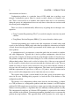
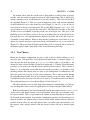
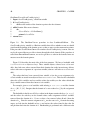
A reduced ordered binary decision diagram (BDD) is a representation of a Boolean expression. A Boolean expression is made of a set of Boolean variables, the operators disjunction,
conjunction, implication, bi-implication and negation, and the constants true and false (1
and 0). Parenthesis can be used around parts of an expression to prevent it from being ambiguous.
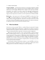
Example: (x1 ∧ x2 ) ⇔ x3 is a Boolean expression. This expression is valid when x1 and x2
and x3 equals true, or when one or both of x1 and x2 is false, and x3 is false.
A binary decision diagram is a data structure which represents a Boolean function f
with linearly ordered Boolean variables. It can be described as a rooted, directed acyclic
graph with nodes and two end terminals, one for 1 (true) and one for 0 (false). A node
is labeled with a Boolean variable and has two edges. Each edge is connected to either a
following variables node, or to one of the end terminals. One of the edges is called ”high”
which represent the Boolean value 1, and the other one ”low” which represent the Boolean
value 0. All paths through the graph respects the variable ordering. The function f is true
only if the given assignment of the variables is valid.
To check whether or not an assignment of the variables is valid, one traverses the graph
5
6
CHAPTER 2. BACKGROUND
following the variable ordering. Selecting the assignment true for a variable is done by
following the high edge of the node representing this variable. When the assignment should
be false, the low edge is selected. At the end of the graph, the end terminal is reached, and
it gives the result. If the path ends up in the end terminal 1 (true), the assignment is valid.
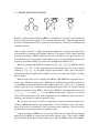
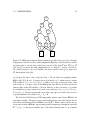
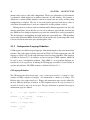
Figure 2.1 shows the BDD graph for the Boolean expression example we introduced above.
X
Y
Z
Z
1
0
Figure 2.1: A BDD of the Boolean expression example. It is easy to find out which solutions is valid.
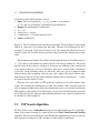
When we are talking about BDDs in this thesis, we actually mean Reduced Ordered
BDDs. Ordered means, as mentioned earlier, that the graph is ordered in such way that all
paths respect the variable ordering. Reduced means that it do not exist two distinct nodes u,
v with the same variable label, and the same high and low succeeding nodes. It also means
that if both the high and low edge of a node u is connected to the same succeeding node, u
is redundant, and hence removed. If a node is missing for the next variable, it means that
both high and low leads to the same node. Because of the reductions the number of nodes
in a BDD is often smaller than the number of different truth assignments of the function it
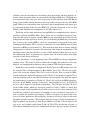
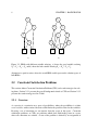
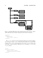
represents. Figure 2.2 shows graphical examples of variable ordering and the reductions.
ROBDDs are canonical [3], which is a big advantage. Multiple BDDs can be represented in a single multi-rooted graph, which gives space savings since all common subgraphs of the BDDs are shared. The equality check of the BDDs can be done in constant
time, since they then have to share the same root-node.
The variable ordering is very important when building the BDD structure. The size
of the structure can be exponential if the variable ordering is bad, but in many cases it is
possible to get a structure of polynomial size. To find the best variable ordering is a NPhard problem in itself. It is even NP-hard to find a variable ordering which gives a structure
2.1. BINARY DECISION DIAGRAMS
X
Y
7
X
X
X
Z
a)
b)
c)
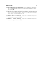
Figure 2.2: Ordering and reduction of BDDs. a) Variables not ordered. Y and Z should not
be at the same level in the graph. b) Two distinct duplicate nodes. This sub-graph should
be shared. c) Both high and low is connected to the same node. The node is redundant and
should be removed.
with less than a constant ”c” bigger size than the optimal size. In many cases there exists
good heuristics for getting good variable orderings. For instance, if the variable ordering
is chosen according to which variables are close to each other in the expression, the size
would in most cases be polynomial. Some functions gives an exponentially increasing size
regardless of variable ordering, for instance the multiplication function [28].
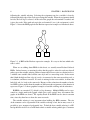
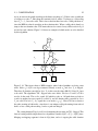
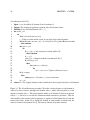
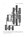
We can for example take the Boolean expression: (X1 ∧Y1 )∨(X2 ∧Y2 ). With the variable
ordering X1 < Y1 < X2 < Y2 , the graph will grow polynomially, but if we use the variable
ordering X1 < X2 < Y1 < Y2 the graph will grow exponentially. This is due to the lack of
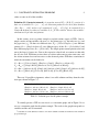
information of what assignment the variables can have at an early state. Figure 2.3 shows
the two graphs.
Boolean expressions can be compiled into BDDs. Each BDD then represents the solution space of Boolean expressions. Furthermore, all Boolean operations can be done
on two BDDs in time proportional to the product of their size, O(|b0 | ∗ |b1 ). To find the
solution space given by a conjunction of the Boolean expressions, we can then run the
conjunction operator on the BDDs, and we get a BDD Bs representing the expression
e = e1 ∧ e2 ∧ . . . ∧ en where e1 . . . en are the Boolean expressions. Using Bs we can now
easily check whether there exists valid assignments or not, whether the expressions form a
tautology, and whether a certain assignment is valid.
The two first cases can be checked in constant time, since the reduction in both cases
results in a BDD with only the end terminal 0 or 1: the end terminal 0 if no valid assignments exist, and the end terminal 1 it the expressions form a tautology. The last case can
be checked by traversing the graph, as explained earlier.
Logical operations on BDDs can viewed as operations on sets of data. The conjunction
operator on two BDDs is equal to the intersection operator of sets. The result is a BDD
derived from the intersection of the solution space of the two BDDs. In the same manner,
8
CHAPTER 2. BACKGROUND
X1
X1
Y1
X2
X2
X2
Y1
Y2
0
Y1
Y2
1
Y2
0
a)
1
b)
Figure 2.3: BDDs with different variable ordering. a) shows the good variable ordering
X1 < Y1 < X2 < Y2 , and b) shows the bad variable ordering X1 < X2 < Y1 < Y2 .
disjunction is equal to union, where the result BDD would represent the solution space of
both BDDs.
2.2
Constraint Satisfaction Problems
This section defines Constraint Satisfaction Problems(CSPs) and search strategies for solving them. Section 2.2.1 presents the overall background related to CSPs and Section 2.2.2
presents the search strategy used in CLab#.
2.2.1
Overview
A constraint is a restriction on a space of possibilities, where the possibilities is a finite
set of variables with associated domains which limits the possible values for the variables.
By using a set of constraints we can narrow down the scope of this space. Constraint
satisfaction problems, or CSPs, are problems which deals with finding states in a space
where all constraints are satisfied. A state of the problem is defined by an assignment of
2.2. CONSTRAINT SATISFACTION PROBLEMS
9
values to some or all of the variables.
Definition 2.1 (Constraint network) A constraint network ℜ = {X, D,C} consists of a
finite set of variables X = {x1 , . . . , xn }, the Cartesian product D over their finite domains
{D1 × D2 × . . . × Dn } and a set of constraints C = {C1 , . . . ,Ct } [10]. A constraint Ci is a
relation Ri defined on a subset of variables Si , Si ⊆ X. The relation1 denotes the variables’
simultaneous legal value assignments.
In this section, we use a printer example to explain various aspects of CSPs. Our example consists of four variables, the user (x1 ), the printer type (x2 ), the ink to use (x3 ) and
the paper size (x4 ). We have two different users, D1 = {Visitor, Employee}, two different
printers, D2 = {Simple, Advanced}, two different types of ink, D3 = {Color, Black} and
three different paper sizes, D4 = {A3, A4, A5}. The simple printer cannot print in colors and
not to the large A3 paper size. Due to the expensive colored ink, we cannot use that with
the A3 size at all. From time to time, there are visitors who wants to print some notes, and
the visitor accounts does not have access to the advanced printer. With these restrictions in
mind, the constraints can be defined as
C1 = R12 = {(Visitor, Simple), (Employee, Simple), (Employee, Advanced)},
C2 = R23 = {(Simple, Black), (Advanced,Color), (Advanced, Black)},
C3 = R24 = {(Advanced, A3), (Simple, A4), (Advanced, A4), (Simple, A5), (Advanced, A5)},
C4 = R34 = {(Black, A3), (Color, A4), (Black, A4), (Color, A5), (Black, A5)}.
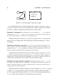
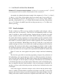
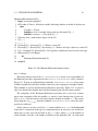
There are 24 possible assignments, where 8 are valid solutions and they form the solution space shown in Figure 2.1
(Visitor, Simple, Black, A4)
(Employee, Advanced, Black, A3)
(Employee, Simple, Black, A4)
(Employee, Advanced, Color, A4)
(Employee, Advanced, Black, A4)
(Employee, Simple, Black, A5)
(Employee, Advanced, Color, A5)
(Employee, Advanced, Black, A5)
Table 2.1: Solution space for the printer example
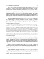
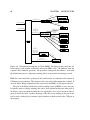
To visually present a CSP we can view it as a constraint graph, and in Figure 2.4 we
can see a constraint graph for the printer example. The nodes in the graph corresponds to
variables and the arcs to constraints.
1 Constraints
are often defined as relations on D, but in CLab# constraints are defined as rules written in
propositional logic
10
CHAPTER 2. BACKGROUND
X1
X2
X3
X4
x1 - User
x2 - Printer type
x3 - Ink
x4 - Paper size
Figure 2.4: Constraint graph for the printer example
An assignment that does not violate any constraints is called a consistent or legal assignment. A complete assignment is one in which every variable is included, and a solution
to a CSP is a complete assignment that satisfies all the constraints [10].
Definition 2.2 (Assignment) An assignment of a set of variables {xi1 , . . . , xik } is a tuple of
ordered pairs (hxi1 , ai1 i, . . . , hxik , aik )i, where each pair hx, ai represents an assignment of
the value a to the variable x, and where a is in the domain of x.
Looking at the printer example, let us say that we assign the user as a visitor and the
printer type to be a simple printer. We will then have the partial assignment (hx1 , Visitori,
hx2 , Simplei).
Definition 2.3 (Satisfying a constraint) Let S ⊆ X be a set of variables included in a constraint, and R be the relation denoting the variables’ simultaneous legal assignments. An
assignment (hxi , ai i, . . . hxm , am i) satisfies a constraint Cn iff it is defined over all the variables in S and the components of the assignment are present in R.
Looking back at the formulation of the printer example, then the assignment (hx1 , Visitori,
hx2 , Simplei) satisfies R12 because its projection on {x1 , x3 } is (Visitor, Simple), which is an
element of R12 . On the other side, the assignment (hx1 , Visitori, hx2 , Advancedi) does not
satisfy the constraint because (Visitor, Advanced) is not an element of R12 .
Definition 2.4 (Consistent partial assignment) A partial assignment (hx1 , a1 i, . . . , hxi , ai i)
is consistent if it satisfies all the constraints C0 ⊆ C which have all of their variables assigned. A partial assignment can also be abbreviated to ~ai , which states all previous assignments up to the current variable xi .
Taking another look at the printer example, the partial assignment (hx1 , Visitori, hx2 , Simplei,
hx3 , Blacki) is a consistent partial assignment because it satisfies all the constraints C0 =
{C1 ,C2 } by projection. The projection on {x1 , x2 } is (Visitor, Simple) and the projection on
{x2 , x3 } is (Simple, Black) and they are both in their respective relations.
2.2. CONSTRAINT SATISFACTION PROBLEMS
11
Definition 2.5 (Constraint network solution) A solution of a constraint network C = {X, D,C}
is an assignment ~a of all its variables X that satisfies all the constraints C.
An example of a solution for the printer example is the assignment (hx1 , Visitori, hx2 , Simplei,
hx3 , Blacki, hx4 , A4i). Here all the variables have been assigned, and we can see that it satisfies all constraints by projection. The projection on {x1 , x2 } is (Visitor, Simple) which is
part of R12 , the projection on {x2 , x3 } is (Simple, Black) which is part of R23 , the projection
on {x2 , x4 } is (Simple, A4) which is part of R24 and the projection on {x3 , x4 } is (Black, A4)
which is part of R34 .
2.2.2
Search strategies
To find a solution to a CSP we can use a number of available search strategies, each involving some sorts of backtracking. The basic idea of backtracking search is to assign
values to variables in a fixed variable ordering. Starting with the first variable, the search
assigns a tentative value for each variable in turn. Before continuing to the next variables,
the search verifies that the assignments are consistent with the previous assignments. If the
search encounters a variable where there are no valid values in the domain, i.e. no value for
that variable are consistent with the previous variable assignments, the search encounters
a dead-end and backtracks. Backtracking means that the search takes a step back in the
variable ordering and selects a new value for the variable preceding the dead-end before
continuing. The search ends either when a required number of solutions is found, or when
the conclusion is that there exists no solutions for the CSP. Backtracking requires only linear space, but in the worst case it requires time exponential in the number of variables [10].
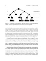
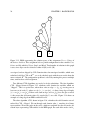
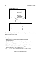
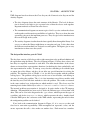
Figure 2.5 shows the search graph for the printer example with basic backtracking
search.
There has been great effort in constraint programming to improve the performance of
the backtracking, and in general there has evolved two different procedures for improvement, look-ahead and look-back [10]. Both of these improve the basic backtracking procedure by reducing the size the the explored search space. The difference lies in when they do
it: Look-ahead procedures are generally employed before the search, and look-back procedures are employed when the search encounters a dead-end and prepares to backtrack. In
our thesis, we focus on the look-ahead procedure, and thus leaves look-back for the reader
to investigate.
As the name suggests, look-ahead strategies seek to discover how the current assignments to variables will affect further assignments in the future search [10]. As the search
progresses the decision to keep or reject an assignment for the current variable is done by
looking at the future variables and how the assignment would affect them. If the assign-
12
CHAPTER 2. BACKGROUND
x1
{Visitor, Employee}
x2
{Simple, Advanced}
x3
{Color, Black}
x4
{A3, A4, A5}
Figure 2.5: Backtracking of printerExample. Bold lines shows the search path to the first
solution, rectangles represent dead-ends, and circles represent assignments
ment, based on the current constraints, empties the domain of one or more future variables
it will reject the assignment and try the next possible value in the domain of the current
variable. If we run out of possible values for the current variable, we will have to backtrack
to the previous variable and try another assignment for that variable. Figure 2.6 presents
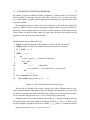
the G ENERALIZED -L OOK -A HEAD procedure for look-ahead search [10]. The procedure
copies the domain values to tentative domains (see line 3) to be able to restore the domains
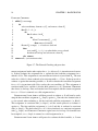
in the event of backtracking. As we can see, the procedure uses F ORWARD -C HECKING to
find legal assignments to the variables, and that sub-procedure is presented in Figure 2.7.
It is quite easy to see how this improves on backtracking. We can see that if the entire
domain of a future unassigned variable is emptied, the search already knows that the current
assignments does not belong to a solution and can backtrack. This leads to the knowledge
that dead-ends occurs earlier in the search process and that a smaller portion of the search
space is explored. Additionally, by the fact that look-ahead removes inconsistent values
from the variable domains throughout the search, we do not have to test the consistency of
the current variable assignment with previous variables.
Different heuristics can be used to further improve the algorithm [10]. Let us say that we
use a dynamic variable ordering. The information gathered during Forward Checking can
then be used to choose the next variable to branch on. In most cases, the most advantageous
is to branch on to the variable that maximally constraint the rest of the search space. This
would be the most constrained variable with the least number of legal values. Another
option is to use heuristics to choose the next value to assign to the next variable. When
searching for a single solution, the best option is to choose the value which maximizes
2.2. CONSTRAINT SATISFACTION PROBLEMS
13
the number of options available for future assignments. A third option is to be aware of
domains which are left with only one valid value. In these cases, we know that there
are no other options available, and the algorithm can immediately assign that value to the
respective variable.
In our implementation, we have used Forward Checking as the look-ahead strategy. It
provides a limited form of constraint propagation during search, and tests the effect of a
tentatively selected variable value to each future variable separately. If the domain of one
of these future variables becomes empty, the value under testing is not selected and the
algorithm selects the next value in the domain.
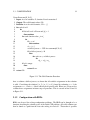
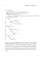
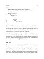
G ENERALIZED -L OOK -A HEAD(X, D,C)
1
2
3
4
5
6
7
8
9
10
11
12
13
14
15
Input: A constraint network with variables X, domains D and constraints C
Output: Either a solution, or notification that the network is inconsistent
0
Di ← Di for 1 ≤ i ≤ n
i←1
while 1 ≤ i ≤ n
do
assign a value to xi ← F ORWARD -C HECKING
if xi is null
then
i ← i−1
(backtrack)
0
reset each Dk ,k > i to its value before xi was assigned
else
i ← i+1
if i = 0 return INCONSISTENT
else return assigned values of {x1 , . . . , xn }
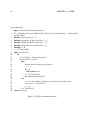
Figure 2.6: The Generalized-Look-Ahead procedure
We can take a look back at the printer example and see how G ENERALIZED -L OOK A HEAD with F ORWARD -C HECKING progresses through it. For simplicity, we can say that
the initial search will return with all domain values intact. If we in the next step2 specifies
a new constraint stating that the user is a visitor, things will get interesting.
G ENERALIZED -L OOK -A HEAD will start by looking at x1 . Forward Checking will start
by testing the first (and only) candidate assignment which is hx1 , Visitori. It will see that
the first candidate assignment for the next variable x2 , hx2 , Simplei is consistent with the
2 Taking
CSPs in multiple steps is a covered in Section 2.3.1
14
CHAPTER 2. BACKGROUND
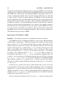
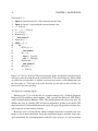
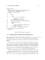
F ORWARD -C HECKING
0
1 while Di is not empty
2
do
0
0
3
select an arbitrary element a ∈ Di , and remove a from Di
4
for all k, 1 < k ≤ n
5
do
0
6
for all values b in Dk
7
do
8
if not C ONSISTENT(~ai−1 , a, b)
0
9
then remove b from Dk
0
10
if some Dk is empty a leads to a dead-end
11
then
0
12
reset each Dk , i < k ≤ n to value before a was selected
0
13
break out of for loop and select next a from Di
14
else return a
15 return null (no consistent value)
Figure 2.7: The Forward Checking sub-procedure
current assignment, but the other option for x2 , hx2 , Advancedi, is inconsistent and remove
it. It then evaluates the assignment for x1 against the first candidate assignment for x3
0
which is Color. This assignment is not consistent and color is rejected from D3 . The next
value for x3 , Black, is then evaluated to be consistent with x1 = Visitor. It then proceeds to
evaluate x1 against the remaining variable, x4 . It will see that the first candidate assignment
for x4 , A3, is inconsistent with Visitor and try the next candidate A4. This assignment is
consistent with Visitor, and this is also the final option for x4 , A5. F ORWARD -C HECKING
then leaves its for-loop. Since no domains have been emptied with the current assignment
for x1 , a = Visitor is returned as a valid assignment for x1 .
G ENERALIZED -L OOK -A HEAD will then proceed to evaluate x2 . It will start by evaluating the first candidate assignment hx2 , Simplei against x3 . Since the first domain value of
x3 was rejected when evaluating x1 , the first and only candidate assignment is hx3 , Blacki.
This assignment is consistent with hx2 , Simplei, and the search proceeds to evaluate x2
against x4 . The first candidate assignment is hx4 , A4i and this is evaluated as consistent
with hx2 , Simplei. The final value for x4 , A5, is also considered as a consistent assignment
with hx2 , Simplei and F ORWARD -C HECKING again leaves its for-loop. No domains have
been emptied, so a = Simple is returned as a valid assignment for x2 .
G ENERALIZED -L OOK -A HEAD will proceed to evaluate the third variable, x3 . It now
2.3. CONFIGURATION
15
contains only a single variable value, Black, and this is evaluated against the two available domain values for x4 , A4 and A5. Both of these are evaluated to be consistent with
hx3 , Blacki and F ORWARD -C HECKING leaves its for-loop. Yet again, no domains have
been emptied and a = Black is returned as a valid assignment for x3 .
G ENERALIZED -L OOK -A HEAD will proceed with the final variable, but since it does
not have any future variables to evaluate against, F ORWARD -C HECKING will return the
first candidate value, a = A4, as a valid assignment for x4 .
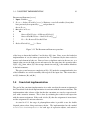
Generalized-Look-Ahead will now return (hx1 , Visitori, hx2 , Simplei, hx3 , Blacki, hx4 , A4i)
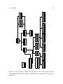
as a solution for the printer example. Figure 2.8 shows the search graph for this search with
bold lines. Normal lines denote the search for all solutions.
x1
{Visitor, Employee}
x2
{Simple, Advanced}
x3
{Color, Black}
x4
{A3, A4, A5}
Figure 2.8: Forward Checking search of printerExample. Bold lines shows the search
path to the first solution, rectangles represent dead-ends, and circles represent assignments.
Dotted lines represent values removed from future variables.
2.3
Configuration
A configuration problem is essentially CSPs put in a multiple step context, where the configuration problem is a set of partial configurations. A configuration tool sets up a configuration problem defined by formal rules so that a user can be guided through a configuration
process towards a final and valid configuration.
Setting a configuration problem in a practical context, consider a product configuration tool where a user through multiple steps ends up with a final valid configuration for
16
CHAPTER 2. BACKGROUND
the product. The configuration process is an iterative process which recalculates the valid
domains for each step in that process.
There are two fundamental requirements for a configuration tool. It must be complete
in the sense that it have to provide the user a route to all valid configurations, and at any
time a free choice between any valid configurations left in the solution space. The other
requirement is that it must be backtrack-free to prevent the user from at any time choosing
a variable assignment for which no valid configurations exists. Finally, a configuration
tool should present results in real-time to facilitate true interactivity. Real-time feedback is
difficult to provide since maintaining the two requirements of completeness and backtrackfreeness together makes computing valid domains a NP-hard problem [11].
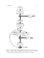
When we talk about configuration tools, we are referring to an interactive process where
a user interactively models a product to his specific needs by choosing options for different
attributes. Every time the user assigns a value to a variable, the configuration algorithm
restricts the solution space by removing all assignments that violate this new condition,
reducing the available user choices to only those values that appear in at least one valid
configuration in the restricted solution space. The user keeps selecting variable values until
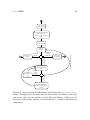
only one configuration is left. This process can be called an interactive configuration [12],
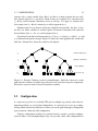
and Figure 2.9 illustrates this process. A configuration tool uses a VALID D OMAINS computation to find the valid domains in a configuration. For each choice the user takes, the
ValidDomains computation should provide all valid values for the variables which has not
been assigned.
I NTERACTIVE -C ONFIGURATION(C)
1
2
3
4
Sol ← S(C)
while | Sol |> 1
do choose (xi = v) ∈ VALID D OMAINS(Sol)
Sol ← Sol ∩ Dxi =v
Figure 2.9: The Interactive-Configuration procedure
As we can see from Figure 2.9, an interactive configuration is an iterative process where
we for each iteration further restrict the available solution space. We start by creating a
initial solution space based on the defined constraints. The process then loops as long as
the solution space is not empty, further restricting the solution space by letting the user
assign values to the variables for each iteration and propagate those changes through the
VALID D OMAINS procedure.
2.3. CONFIGURATION
2.3.1
17
Configuration with CSPs
As presented in Section 2.3, a configuration problem is essentially CSPs in a multiple step
context. The underlying meaning of that is that for each step in the configuration process,
the user makes a choice and assigns a value to a variable. That assignment forms a new
constraint3 Ct+1 in the CSP, C = Ct +Ct+1 .
A CSP used in a configuration problem can be thought of as a dynamic state, where
we for each step in the configuration process get new constraints which are propagated
to represent the new state. By performing constraint propagation we prune the domains
so that any values which, with the current set of constraints, does not belong in any valid
solutions are removed.
When a user makes a choice in the configurator, that choice is the basis for a new constraint which is added to the constraint network. Consider the printer example. When the
user selects the user type to be a Visitor, a new constraint is added to the constraint network
which states that (x1 = Visitor). After the constraint has been added, the configuration
will apply that via constraint propagation through a selected CSP-algorithm and return a
new state, that state being the basis for the next step in the configurator. In CaSPer, these
new constraints are virtual and the propagation of the user choices is done in the VALID D O MAINS U SER C HOICE procedure (covered in Chapter 3.2.1), independently to the constraint
network itself.
To facilitate this process, the search performed by the VALID D OMAINS computation
must search for and return the all current valid domains so that we for each step use the domains resulting from the previous propagation. This behavior of the configurator enforces a
very important property of interactive configuration called completeness of inference. The
user cannot pick a value that is not a part of a valid solution, and furthermore, a user is able
to pick all values that are part of at least one valid solution [12].
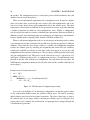
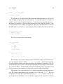
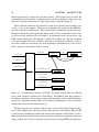
Figure 2.10 shows solving configuration problems using CSP, and Figure 2.11 shows
the VALID D OMAINS procedure for calculating valid domains.
The C ONFIGURATION -W ITH -CSP procedure starts off by calling the VALID D OMAINS
procedure (Figure 2.11) to calculate the initial valid domains based on the constraints in the
configuration problem. This is done with the Boolean variable InitialSearch set to false, so
that we differentiate between the initial search and search operations which occurs after
user assignments. If none of the domains are empty after this initial search, the procedure
continues by looping for as long as there is domains with multiple domain values (or termination of the configuration). In this loop, a user choice is made which assigns a value from
the valid domains to a given variable. When this choice is made, that variables’ domain is
3 In
CLab# this is done by constraining the variable domain to contain only the selected value instead of
creating a new constraint
18
CHAPTER 2. BACKGROUND
C ONFIGURATION -W ITH -CSP(X, D,C)
1 Input: A set of variables X, domains D and constraints C
2 InitialSearch ← T RUE Global Boolean variable
3 D ← VALID D OMAINS(X, D,C)
4 if ∀di ∈ D, size > 0
5
then
6
InitialSearch ← FALSE
7
while ∃di ∈ D, size > 1
8
do choose (xi = v) ∈ di ∈ D
9
di ← {v} Updates D with the reduced domain di
10
D ← VALID D OMAINS(X, D,C)
Figure 2.10: Pseudocode for solving configuration problems with CSP
pruned to contain only that value. The final task in this loop is to compute the new valid
domains before the user is given the option to choose another assignment.
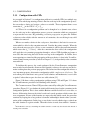
When the VALID D OMAINS procedure is called, it starts of by initializing an empty set
VD which will hold the valid domains. The procedure then iterates through all domains
di ∈ D. Except for the initial execution, all domains which contains a single value will be
skipped, since these are already determined to be consistent in previous searches. Within
this loop, the procedure iterates through all the domain values, and skips those values which
already exist in the valid domains set (V D). This is because these values have already been
evaluated to exist in a consistent assignment by the CSP-A LGORITHM procedure4 . For
each domain value v j , we set the current domain di to consist of only that value and execute
the CSP-A LGORITHM procedure to get a solution to the constraint problem. As long as a
complete solution is returned, we iterate through that solution and copy the assigned values
to their respective domains in the valid domains set, V D. As soon as all the domain values
for the current domain di has been evaluated, the procedure checks to verify that the valid
domain for di is not empty. If it is, we terminate the procedure and return N ULL because no
value in di was valid. After all domains have been evaluated, without any becoming empty,
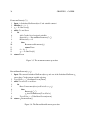
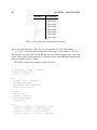
we return the valid domains to the C ONFIGURATION -W ITH -CSP procedure.
As we can see from the VALID D OMAINS procedure, there are some advantageous features which cuts back on unnecessary searching. First, the use of valid domains makes sure
that if a domain value is not included in the valid domains due to not being consistent, it
will not get available later in the configuration process either. The second is that when we
4 In
CLab#, the CSP-A LGORITHM is the G ENERALIZED L OOKAHEAD procedure
2.3. CONFIGURATION
19
VALID D OMAINS(X, D,C)
1 Input: A set of variables X, domains D and constraints C
2 Output: The valid domain values V D
3 Initialize A set for valid domains, V D ← {}
4 for each di in D
5
do
6
if InitialSearch is FALSE and |di | = 1
7
then continue
8
for each domain value v j in di
9
do
10
if v j ∈ vdi
11
then continue
12
di ← {v j }
13
validAssignment ← CSP-A LGORITHM(X, D,C)
14
if |validAssignment| 6= 0
15
then
16
for each vak ∈ validAssignment
17
do
18
vdk ← vdk ∪ vak
19
if vdi is empty
20
then
21
return N ULL
22 return V D
Figure 2.11: The Valid Domains Procedure
have a solution validAssignment, we know that all variable assignments in that solution
is valid. Considering the solution (hx1 , 3i, hx2 , 1i, hx3 , 9i), found by evaluating x1 = 3, the
assignments x2 = 1 and x3 = 9 have allready been proved valid. Hence we do not need to
evaluate those assignments in future steps of procedure. This is covered in line 10 and 18
in Figure 2.11.
2.3.2
Configuration with BDDs
BDDs can be used for solving configuration problems. The BDD can be thought of as a
function describing the solution space of the initial CSP problem. All valid solutions can
then be found as a path from the root node ending in terminal 1. That makes it possible
20
CHAPTER 2. BACKGROUND
to guide the user through the configuration process by using the BDD to reason about the
solution space. To do that, the information in the initial CSP problem has to be precompiled
into a BDD. This is the hard part, since building the BDD is exponential in worst case. If
we have a configuration problem where most of the domain combinations are valid, that
is, where the rules do not lead to many reductions, the BDD has to represent almost all
possible combinations. The worst case number of solutions is the cartesian product of the
average number of domain values: ∏ni=1 (|Di |). This is obviously exponentially based on
the number of variables n. For many problems the number of valid solutions is much less
because of the rules leading to big reductions. If we choose a good variable ordering of
the problem, the size of the graph will become even smaller. In practice BDDs are in many
cases a good tool for solving this type of problems. This part of the chapter will describe
how BDDs can be used to solve configuration problems. First we have to explain how a
CSP problem can be represented as a BDD.
Representing a CSP problem as a BDD
Disclaimer
The following discussion is not within the main focus of our thesis.
To use BDDs for solving a configuration problem, we need to create a Boolean function
of the problems’ solution space. A Boolean encoding of the variables and their domain
values is needed [12, 13]. We can encode domain values as ranges starting from 0. The
domain of Papersize in the Printer Example, the enumeration values A3, A4, A5 are then
encoded as the range [0..2]. A problem range [−3..1] is encoded as the range [0..4]. We
define li as the number of bits required to encode a value v in domain Di . Since each bit
can have the value 0 and 1, li = dlg|Di |e. We can encode every value v ∈ Di in binary
by making a vector of Boolean values: ~v = (vli −1 , . . . , v1 , v0 ) ∈ Bli . Boolean variables are
encoded in the same fashion: ~b = (bli −1 , . . . , b1 , b0 ). An expression assigning a value v for
a variable xi can be represented as the Boolean function given by the binary expression
bli −1 = vli −1 ∧ . . . ∧ b1 = v1 ∧ b0 = v0 . If we look at the Papersize enumeration variable
again, which has domain size 3, l2 would be dlg3e = 2. Thus we can encode A5 as 00, A4
as 01 and A3 as 10. For example, the Boolean function encoding Papersize = A5 would be
b1 = 0 ∧ b0 = 0.
For the Papersize variable we have three possible domain values, and we use two bits
to represent them. Two bits gives us four possible combinations, and in our example the
combination 11 is not used, and therefore not valid. To deal with such cases, we introduce
a Boolean constraint (a domain constraint), which forbids unwanted combinations for all
variables i to n: FD = ∧ni=1 (∨v∈Di xi = v). Considering the Papersize variable, this constraint
would be that it either can be A3, A4 or A5.
Since any expression ϕ innermost consists of nested xi = v expressions with operators
2.3. CONFIGURATION
21
between, we can build the Boolean function representing ϕ by translating each xi = v and
apply operators between the results. The translate function τ does this job. It can be defined
inductively as:
τ(xi = v) ≡ (~bi =~v)
τ(ϕ ∧ ψ) ≡ τ(ϕ) ∧ τ(ψ)
τ(ϕ ∨ ψ) ≡ τ(ϕ) ∨ τ(ψ)
τ(¬ϕ) ≡ ¬τ(ϕ)
where ψ is another expression.
Running the τ f unction on all rules f ∈ F, gives us m Boolean functions representing
the solution space of each of them. What we want is a BDD representing a Boolean function
S̃(C) of the solution space S(C). To do that we need a BDD function τ̃, which converts the
Boolean functions of the rules and the domain constraint FD into BDDs. When we have the
BDD versions, S̃(C) can be achieved by the following operation:
S̃(C) ≡ ∧m
i=1 (τ̃( f i )) ∧ τ̃(FD ).
That is: All the BDDs representing each rule f i is conjoined together. In the end
the BDD representing the domain constraint FD is conjoined with the result, to prevent
insignificant bit values to be a part of the solution space.
Using a BDD for finding a backtrack free configuration
After compiling the initial CSP problem into a BDD representing the solution space S̃(C),
the user can start solving the configuration problem: The user is presented with the valid
domain values. The values are calculated out of the BDD using two different algorithms,
which are described in a section later in this chapter. Since the BDD represents a function
which is true only for valid assignments, the user is only presented with domain values
which leads to a backtrack free configuration. When the user assigns a domain value v for
a certain variable xi , this can be thought of as an extra rule which is converted to a binary
expression eϕ . A BDD representing this expression is made, and thus representing the solution space of this rule S̃(eϕ ). The initial BDD is conjoined with the expression BDD and we
get a new BDD representing the solution space S̃(C ∩ eϕ ). The valid domains calculation is
done once more, and the user is presented with the remaining valid domains. The user continue to extend the partial configuration by choosing a domain value. This is done until the
BDD is reduced to only contain one valid solution, and we have a full configuration. The
configuration procedure is described generally for configuration problems in Figure 2.9.
22
CHAPTER 2. BACKGROUND
The conjunction of two BDDs is an operation which is polynomial in the size of the
BDDs. Since a BDD can be of exponential size this operation will in the worst case take
exponential time, and thus the generation of the solution space can be hard and take a long
time. A solution to this problem is to compile the solution space of the problem in an offline
phase. The resulting solution space will in many cases be small, even if the precompilation
process takes exponential time. For most real world problems this is true. Since this part
can be performed offline, the user will not be aware of how long time this takes. Hence
BDDs could be a very good choice irrespective of how long time it takes to run the initial
compilation. The computation of valid domains, which is performed in the online phase,
is also polynomial in the size of the BDD. Therefore we can not guarantee the response
time to the user. But if the resulting BDD from the offline phase is small, as it is in most
cases, the interactive phase has a polynomial and thus a short response time. After the
precompilation is done we know the size of the BDD representing the solution space, and
we can therefore predict the running time of the online phase.
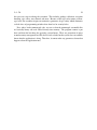
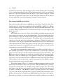
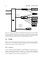
Example: For the printer example we get the BDD in Figure 2.12 representing the
solution space of the problem. The four variables are encoded as follows:
User: x10 where 0 encodes Visitor and 1 encodes Employee
Printer: x20 where 0 encodes Simple and 1 encodes Advanced
Ink: x30 where 0 encodes Color and 1 encodes Black
Papersize: x41 and x40 where 00 encodes A3, 01 encodes A4 and 10 encodes A5 (11 is
invalid, and thus taken care of by the domain constraint FD )
After calculating the valid domains of this graph, the user is presented the valid domains
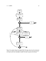
as shown in Figure 2.1. Let us now assume that the user chooses the value Visitor for the
User variable. A BDD for the rule User = Visitor, or with the BDD variable encoding
x10 = 0, is made. Conjoined with the initial graph, we get a new BDD shown in Figure 2.13.
The graph is much smaller, and we are closer to a full configuration. The high edge of x10
now goes straight to the terminal 0 node, which means that User = Employee no longer is
a part of a valid configuration.
Calculating valid domains [11]
Disclaimer
The following discussion is not within the main focus of our thesis.
For each new BDD, the valid domains have to be calculated. X ji defines a BDD variable
where i corresponds to a CSP variable index, and j corresponds to a BDD variable index
encoding the i − th CSP variable. Xb is a set of ordered Boolean variable indexes. Each X ji
corresponds to a unique index k ∈ Xb , where Xb is a set of Binary variable indexes. The
1
2
ordering of Xb follows the rule X ji1 < X ji2 iff i1 < i2 or i1 = i2 and j1 < j2 . The function
2.3. CONFIGURATION
23
X10
X20
X20
X30
X30
X41
X41
X40
1
X40
X40
0
Figure 2.12: BDD representing the initial solution space of the Printer Problem. All paths
ending up in terminal 1 encodes a valid configuration. High lines (solid drawn lines) encode
the binary value 1, and low lines (dotted lines) encode 0. The path X10 high, X20 high, X30
high and X41 low encode the valid configurations User = Employee, Printer = Advanced,
Ink = Black and Paper = A3 or A4. Both A3 and A4 are encoded, since X41 low jumps over
X40 , thus both has to be valid.
var1 (k) gives the index i and var2 (k) the index j. We can define our compiled problem
BDD as B(V, E, Xb , R, var). Vi denotes the set of all nodes u ∈ V , which encodes a certain
CSP variable Xi . (Vi = u ∈ V | var1 (u) = i). With u in var1 (u) we mean the index k that
node u maps to. Vi defines a layer in the BDD graph, since this set of nodes encodes the
domain values of the CSP variable xi . We also define Ini as the set of nodes u ∈ Vi which
are reachable by an edge, connected to a node in an earlier layer: Ini = {u ∈ Vi | ∃(u0 , u) ∈
E.var1 (u0 ) < i}. Since the root node R does not have any edges to an earlier layer we need
a special definition for it, which is: Ini0 = Vi0 = R.
The Calculate Valid Domains (CVD) functionality extracts values from a BDD for all
unassigned variables. The process starts with showing the user the valid domains he can
chose from, calculated by CVD on a BDD we can call Bρold . When a value is chosen, we get
a new, more restricted BDD Bρ , representing a partial assignment ρ, through the operation
Bρold ∪ (x, v). x is the chosen variable, and v is the chosen domain value. (x, v) is marked
24
CHAPTER 2. BACKGROUND
X10
X20
X30
X41
X40
X40
1
0
Figure 2.13: BDD representing the solution space of the assignment User = Visitor of
the Printer Problem. This assignment led to a partial configuration for the variables User,
Printer and Ink, which is Visitor, Simple and Black. Total number of solutions in this graph
is two, since Paper can be selected to either A4 (01) or A5 (10).
as assigned, and are skipped by CVD. Domain values for unassigned variables, which were
calculated valid by CVD on Bρold , are to be checked again with the new results from the
more restricted Bρ . The configuration problem is solved by running this process multiple
times, until we have a full assignment.
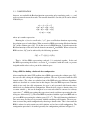
Two different CVD algorithms are needed to do the calculation. The first algorithm,
CVD - Skipped shown in Figure 2.15, calculates valid domains for variables which are
”skipped”. This is a special case, where there exist an edge e = (u1 , u2 ) crossing over at
least one set of nodes V j , where var1 (u1 ) < j < var1 (u2 ). e is then a long edge of length,
|e| = var1 (u1 ) − var1 (u2 ). If there exist such an edge, and var1 (u2 ) does not give terminal
0, this means that all domain values D j encoded by V j are valid. Figure 2.14 shows an
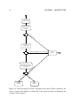
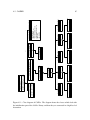
example of a long edge from BDD variable X0 to Z0 .
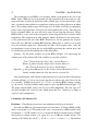
The other algorithm, CVD, shown in figure 2.16, calculates the valid domains not calculated by CVD - Skipped. We run through each domain value j, encoding it to binary
representation. We use the nodes in the set Ini , which we can think of as the root nodes of a
certain layer representing CSP variable i in the BDD graph. For each of the nodes u in Ini ,
2.3. CONFIGURATION
25
we try to traverse the graph according to the binary encoding of j. If there exist a path from
u leading to a node u0 , other than the terminal node 0, where u0 belongs to a succeeding
layer Vl , i < l, j has to be valid. This is due to the fact there has to be a valid path from u0 ,
since the BDD is reduced according to the reduction rules. When a valid path is found, we
jump to the next domain value. This means that we do not need to try all the nodes in Ini if
we find an early solution. Figure 2.14 shows an example of which nodes are to be checked
by this algorithm.
X1
u0
Vx
X0
u1
Y1
u2
Vy
Vz
Y0
Z0
1
u4
Z0
u3
u5
0
Figure 2.14: This figure shows a BDD example where both algorithms are doing some
work. Node u1 ’s high is an edge connected directly to node u4 , and layer Vy is skipped.
Therefore all domains encoded by layer Vy , in this case the values 00, 01, 10 and 11, have
to be valid. The algorithm CVD - Skipped takes care of this. For layer Vx and Vz CVD is
used to do the work. The set Inx equals {R} which is node u0 . All paths from u0 leads to
a node in another layer not equal to terminal 0, and all domain values encoded by layer
Vx are valid. For layer Vz , Inz equals the set of nodes {u2 , u3 }. Here CVD has to traverse
the paths starting in both nodes, since there is one unique valid path starting from each of
them. u2 has a valid path encoding 1 and u3 a path encoding 0.
The sorting function TopologicalSort is dominating the run time of CVD - Skipped. This
form of sorting could be implemented as a depth first search in O(|E| + |V |) = O(|E|) time.
Merging overlapping segments is done in O(n) time, and so is copying the valid domains
26
CHAPTER 2. BACKGROUND
CVD - S KIPPED (B)
1
2
3
4
5
6
7
8
9
10
11
12
13
14
15
16
17
18
19
20
21
22
23
24
Input: The BDD B that the calculation should be performed on
Initialize a List for saving each CSP variables longest edge
for each variable index i = 0 to n − 1
do Li ← i + 1 Each variables edge has at least to be connected to the next CSP variable
T ← T OPOLOGICAL S ORT(B)
for each tk ∈ T
do
u1 ← tk , i1 ← VAR1 (u1 )
for each u2 ∈ A DJACENT(u1 )
do
Li1 ← M AX{Li1 ], VAR1 (u2 )}
S ← {}, s ← 0
for each i = 0 to n − 2
do
if i + 1 < Ls
then Ls ← M AX{Ls , Li+1 }
else
if s + 1 < Ls
then S ← S ∪ {s}
s ← i+1
for each j ∈ S
do
for i = j to L j
do V Di ← Di
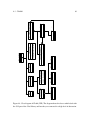
Figure 2.15: CVD - Skipped algorithm in pseudo code. From line 3 to 11 the algorithm
records the longest edge for each variable, and stores the results in Li , where i is the CSP
variable encoded in layer Vi . In lines 12 to 20 overlapping long segments are merged.
We can think of this as two or more long edges overlapping each other, originating from
different layers. Such overlapping edges is represented as a long segment, where all domain
values encoded in the layers between the start point and end point has to be valid. The last
part of the code copies all the domain values of the skipped variables into the valid domains
structure.
2.4. C#
27
CVD(B, xi )
1 Input The BDD B that the calculation should be performed on
2 Input a variable xi , the CSP variable for which valid domains should be calculated
3 V Di ← {}
4 for each j = 0 to |Di | − 1
5
do
6
for each uk ∈ Ini
7
do
8
u0 ← T RAVERSE(uk , j)
9
if u0 6= T0
10
then
11
V Di ← V Di ∪ { j}
12
return
Figure 2.16: CVD algorithm in pseudo code. This algorithm runs through each domain
value j for a certain variable xi , and for each internal root node of the layer Vi , u ∈ Ini .
For each such value j and node u the Traverse algorithm 2.16 is used. If the result from
Traverse is a node u0 , j has to be valid, and the value is copied into the valid domains
structure. When the first solution of j is found, CVD jumps to the next domain value. If the
result from Traverse is terminal 0 for all nodes in Ini , j is not valid.
results. The complexity of this algorithm is therefore O(|E| + n). The CVD algorithm is
run one time for each layer Vi in the graph. Together with Traverse it traverses through each
node in the layer one time for each domain value j. Thus the complexity for running it on
one layer Vi on all domain values in that layer Di has to be O(Vi · Di ). Total running time
for all variables n then has to be: O(∑n−1
i=0 |Vi | · |Di | + |E| + n).
2.4
C#
This section presents the development language used in CLab#, and the idea of managed
code.
C# [20] is an object-oriented programming language developed by Microsoft as a part
of their .NET initiative, and is an evolution from Microsoft C and Microsoft C++. It is
designed to be simple, modern, type safe and object-oriented. C# code is compiled as
managed code, which means it benefits from the services of the common language runtime.
These services include language interoperability, garbage collection, enhanced security,
28
CHAPTER 2. BACKGROUND
T RAVERSE ( U , J )
1
2
3
4
5
6
7
8
9
10
11
12
13
14
15
16
17
18
19
Input An internal root node u of the currently checked layer
Input An integer j representing the current domain value
i ← VAR1 (u)
v0 , . . . , vki−1 ← E NC( j)
s ← VAR2 (u)
if Marked[u] = j
then return T0
Marked[u] ← j
while s ≤ ki − 1
do
if VAR1 (u) > i
then return u
if vs = 0
then u ← L OW(u)
else u ← H IGH(u)
if Marked[u] = j
then return T0
Marked[u] ← j
s ← VAR2 (u)
Figure 2.17: Traverse used by CVD for traversing the graph. It returns the node the traversal
ends up in, either the terminal node 0, or the first node u0 in a succeeding layer. Nodes which
are visited for a certain value j is marked, to prevent it to traverse a node multiple times for
the same value of j. The same node would obviously give the same results each time it is
traversed for the same encoding.
and improved versioning support.
Managed code [1] is code that has its execution managed by a Common Language
Interpreter(CLI)-compliant virtual machine (VM), typically the Microsoft .NET Framework Common Language Runtime (CLR). This management involves that at any time, the
runtime may stop an executing CPU and retrieve information specific to the current CPU
instruction address. Information that must be query-able generally pertains to runtime state,
such as register or stack memory contents.
Before the code is executed by the VM it is compiled into native executable code, also
known as Just-in-time compilation. Since this compilation happens internally in the managed environment, the environment knows what the code is going to do, and can perform
2.4. C#
29
the necessary steps involving the execution. This includes garbage collection, exception
handling, type safety, array bounds and more. Because of the type safety nature of managed code, the execution engine can maintain a guarantee of type safety which eliminates
a whole class of programming mistakes that often lead to security holes.
If we take a look at unmanaged code, we can see that the unmanaged executable files
are basically binary x86 code loaded directly into memory. The program counter is put
there and thats the last thing the operating system knows. There are protections in place
around memory management and I/O devices and so forth, but the system does not actually
know what the application is doing. Therefore, it cannot make any guarantees about what
happens when the application runs.
30
CHAPTER 2. BACKGROUND
Chapter 3
CaSPer
3.1
Overview
In this chapter we provide technical description of the CaSPer library (see Section 4.2).
We provide pseudocode and explanations of the algorithms and data structures we have
used, how they solve the main task of this library and why we have made the choices we
have. In short, the CaSPer library contains the Valid Domains computation, the main CSP
forward checking algorithm for search, data structures that support effective backtracking
and restoration of domains, implementation of constraint expressions, variable ordering
and consistency check classes.
3.2
Valid Domains Computation
The main purpose of the CaSPer library is to provide CSP search functionality to support
configuration. This process is divided into two main routines: the valid domains procedure,
and the CSP search algorithm.
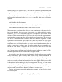
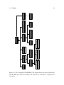
The VALID D OMAINS procedure is the outer loop in the configuration process, as described in Section 2.3.1. The algorithm is shown in Figure 3.2. It is found in class CSP
which is the interface of the library, and runs the search algorithm of CaSPer. The procedure runs through all values v j of all domains di in the constraint problem, reducing domain
di to contain only v j , as seen on line 14 in Figure 3.2. The CSP algorithm then searches
for a valid assignment on all domains including the currently reduced domain di ∈ D. The
result returned from the search algorithm is either a complete valid assignment ρ or N ULL,
depending on whether or not the partial assignment of value ρi = {v j , xi } could be extended
to a full valid assignment.
31
32
CHAPTER 3. CASPER
All domain values from the search result is then marked as valid for their respective
variable, since the returned assignment represents a full configuration. This is achieved by
adding each value to a set of valid domains vdi for each variable xi . This is done in line 20 of
the algorithm (Figure 3.2). This set is used in future steps of the valid domains algorithm
to check whether or not a value should be tested (Figure 3.2, line 12), as we do not test
values that have already been found valid. We used the IESI.Collection HybridSet [23]
representation of a set to represent the valid values. The HybridSet can take on the form
of either a list or a hashtable, depending on the size of the input data. This gives us the
flexibility we need in CLab#, as there is no way of predicting the size of the input data set.
For small data sets, a list implementation is known to be faster, but as the data set grows,
a hashtable is more efficient. When we have finished searching for valid values in di , we
update di to include only those values found in the valid domains set vdi , as seen on line 24
(Figure 3.2). This means that all illegal domain values for di is removed, and we will never
check them again in future interactions of the VALID D OMAINS procedure.
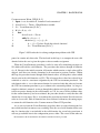
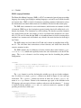
3.2.1
User Choices
During the interactive configuration, the user is able to choose which variables to set at
any given time. This procedure, VALID D OMAINS U SER C HOICE, is shown in Figure 3.1.
Once the user has made his choice ρu = {vu , xu }, i.e selected value vu of variable xu , the
domain Du of the selected variable is reduced to contain only vu . Then the VALID D OMAINS
procedure is run again, now with the chosen variable domain reduced. This is shown in
Figure 3.1. It is important to note that when we run this procedure, it is possible to skip
checking domains that contain only one value as our configuration is backtrack-free and
hence this value has to be part of some valid assignment. This is made possible through
the global Boolean variable InitialSearch which is initially set to true before running the
VALID D OMAINS the first time and then set to false by VALID D OMAINS U SER C HOICE.
This configuration process is described in Figure 2.10 in Section 2.3.1.
The choice whether or not to omit single valued domains is implemented as a C# property, meaning that it can be set by the application or developer using the CaSPer library.
Both VALID D OMAINS and VALID D OMAINS U SER C HOICE return a list of CasperVarDom
objects, where each object contains a set of valid domain values and a set of domain values
for a given variable. This is a representation of domains and variables that are adequate for
the VALID D OMAINS method. As we run the configuration procedure, the internal representation of variables and domain values is altered so that invalid domain values are removed
from the domain values set, and valid domain values are added to the valid domain set. In
this manner, values already marked valid and removed values will not be checked again
later.
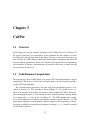
3.3. CSP SEARCH ALGORITHM
33
VALID D OMAINS U SER C HOICE(ρu , X, D,C)
1
2
3
4
5
6
Input: An user assignment ρu = {vu , du } of value vu from domain
du ∈ D, and a set of variables X, Domains D and constraints C
Output All valid domains ValidDomains
du ← {vu }
InitalSearch ← FALSE
validDomains ← VALID D OMAINS (X,D,C)
return validDomains
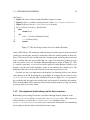
Figure 3.1: The VALID D OMAINS U SER C HOICE procedure. The user chooses value vu from
domain du , and forces du to contain only that value. Then the VALID D OMAINS (X,D,C)
procedure is run again on the altered domain set D. By setting the global InitialSearch
variable to false, the VALID D OMAINS procedure skips domains that contain only a single
value.
The maximum total number of iterations considering both loops in VALID D OMAINS is
n−1·|D|, where n is the number of variables and |D| is the average domain size. The reason
for this is that, in the worst case situation we do not get any reductions of the domains and
every domain value has to be tested. The first results gives n domain values, which have
to be valid. In the following round, we will in the worst case get an assignment which
differs from the first assignment with only one value, which is the tested domain value.
That means we have to test each of the remaining domain values except for the n − 1 values
we found in the first round of search.
However, due to the nature of CSP problems, reductions in the valid domains often
occurs. By including the mechanisms to mark valid domain values and skip invalid as
well as singleton domain values during the configuration process, we can then speed up the
CSP search for each round in VALID D OMAINS, as well as the VALID D OMAINS procedure
itself. This increases the efficiency when checking whether or not a partial assignment can
be extended to a full assignment.
3.3
CSP Search Algorithm
We have chosen to use a look-ahead strategy for our implementation of the search algorithm. For forward checking we settled for the basic Select-Value-Forward-Checking
procedure. The reason for this choice is the fact that this algorithm has proven to work very
well in practice in many cases [10], and that it is rather simple to implement.
34
CHAPTER 3. CASPER
VALID D OMAINS(X, D,C)
1
2
3
4
5
6
7
8
9
10
11
12
13
14
15
16
17
18
19
20
21
22
23
24
25
Input: A set of variables X,domains D and constraints C
Output: The domains D, updated to contain only valid domain values
Initialize A List Of Valid Domains VD ← {}
for each di ∈ D
do
Make a local reference di0 to di
: If this is not the initial search, we can skip single valued domains:
if InitialSearch = FALSE ∧ |di | = 1 InitialSearch is a global Boolean variable.
then continue
for each v j ∈ di0
do
if v j ∈ vdi v j has already been found valid for Xi
then Continue
di ← {v j }
valAssign ← G ENERALIZED L OOKAHEAD(X, D,C)
if |valAssign| 6= 0
then
for each vak ∈ valAssign
do
vdk ← vdk ∪ vak Update valid dom of var xk
if vdi is empty
then
return NULL No value v j ∈ di was consistent
di ← vdi
return D The original domains of the variables have been replaced by their valid domains.
Figure 3.2: The VALID D OMAINS procedure. We make a local reference to each domain in
order to be able to traverse through each domain value v j while still being able to set the
domain to contain only v j . This means that the whole set of domains D have been updated
with di ← v j before it is sent into the G ENERALIZED L OOKAHEAD procedure. Then for
each variable in the returned valid assignment, we update its valid domain list vdk with the
current valid value. In line 24 we update the domain of each variable to contain only the
values in its final valid domain list vdi . The altered domains D are then returned.
3.3. CSP SEARCH ALGORITHM
35
The CSP class has its own representation of variables and domains, the CasperVarDom
objects. These objects are given as input to the G ENERALIZED L OOKAHEAD - procedure,
in addition to the constraint representation, implemented as CSPExpr classes. This domain and variable representation is not adequate for the Generalized Lookahead search
algorithm, so we copy the information from the input domains and create new variable and
domain objects of class LookaheadVarDom, that support the algorithm. This includes
methods and data structures that support backtracking and restoration of domain values, as
well as structures for necessary bookkeeping of removed domain values that are not to be
checked later.
The search is performed by an object of class GeneralizedLookahead. This class
has an implementation of procedure L OOKAHEAD, see Figure 3.3, which is the starting
point of the search. The class also implements the procedures S ELECT VALUE (Figure 3.4),
F ORWARD C HECKING (Figure 3.5) and P RUNE N EXT D OMAIN (Figure 3.6), which take
care of different aspects of the search.
In lines 3 to 6 in procedure L OOKAHEAD, a number of empty lists and sets are initialized. These are used by some of methods in the GeneralizedLookahead class. The
assignment list is used to contain the previously assigned variables (those set prior to the
current and next assignments). When a valid value for the current variable xil is returned
by S ELECT VALUE, xil is added to assignment, seen in line 22. If we on the other hand can
not find a valid assignment of xil under the current partial assignment, we remove the last
element in assignment and backtrack. This is because we need to try to assign a different
l
value to variable xi−1
that was the last element in assignment. In the end, if all variables
could be assigned, assignment will represent a single valid solution and is returned by the
L OOKAHEAD procedure.
The hashtable AllRemovedValues defined in line 4 is used in the R EMOVE and BACK TRACK D OMAINS, for keeping track of the removed values during pruning and resetting of
domains. Hashtable ReducedVariables is also utilized by the R EMOVE and BACKTRACK D OMAINS procedures, keeping track of which variables have had their domains pruned by
some variable. No values are stored here, this is just a lookup table to increase efficiency
of BACKTRACK D OMAINS.
Finally, the AssignedVars hashtable is used by the Consistent class. It contains all
variables that have been assigned so far, also including the current and next assignments, so
that we easily can decide whether or not an expression should be checked for consistency
with the current partial assignment.
The most challenging part in the design of the GeneralizedLookahead class is
to provide an efficient and modifiable means of selecting the next variable and value for
testing, as well as implementing efficient procedures for backtracking and restoration of
domains. These concerns will be the emphasis of the following sections.
36
CHAPTER 3. CASPER
L OOKAHEAD(X c )
1
2
3
4
5
6
7
8
9
10
11
12
13
14
15
16
17
18
19
20
21
22
23
24
25
Input: A List of CasperVarDom objects X c
X l ← M AKE L OOKAHEADVAR D OMS(X c ,VarOrder,ConstraintGraph) : Create internal
variable objects
Initialize a list assignment ← {}
Initialize a global Set AllRemovedValues ← {}
Initialize a global Set ReducedVariables ← {}
Initialize a global Set AssignedVariables ← {}
Initialize i ← 0
xil ← X l .G ET VAR(0)
while xil is not N ULL
do
selectedValue ← S ELECT VALUE(xil , i)
if selectedValue is N ULL
then
Remove the last element of assignment
i ← i−1
if i < 0
then return N ULL
l0
xi ← Xl.G ET VAR(i)
BACKTRACK D OMAINS(xil0 )
else
xil was successfully assigned and is added to the assignment list
assignment ← assignment ∪ xil
i ← i+1
l
l
xi = X .G ET VAR(i)
return assignment
Figure 3.3: The L OOKAHEAD procedure
3.3. CSP SEARCH ALGORITHM
37
S ELECT VALUE(xil , i)
1 Input: A LookaheadVarDom object xil and variable counter i
2 SelectedValue ← xil .G ET N EXT VALUE(T RUE)
3 while SelectedValue is not N ULL
4
do
5
if i > 0
6
then
7
previousVar ← X l .G ET VAR(i − 1)
8
R EMOVE(xil , previousVar)
9
xil .A DD T O R EMOVED(SelectedValue)
10
B OOLEAN EmptyDomain ← F ORWARD C HECK(xil , i)
11
if EmptyDomain is FALSE
12
then
13
remove xil from the list of assigned variables
14
return SelectedValue
15
SelectedValue ← xil .G ET N EXT VALUE(FALSE)
16 remove xil from the list of assigned variables
17 return N ULL
Figure 3.4: The S ELECT VALUE procedure
3.3.1
Selecting the next variable and value during search
The responsibility of selecting the next variable has been placed in class LookaheadVariables,
which contain a list of LookaheadVarDom objects. The selection is performed by procedure G ET VAR, which takes as an argument a variable index. The procedure is shown in
Figure 3.7.
The reason we have chosen to put the responsibility of getting the next variable in
the LookaheadVariables class is that we wish to hide the mechanism of getting the
next variable from the algorithm, and support additional means of calculating the variable
ordering. This can be achieved by creating a new variable order class that implements
the IVariableOrdering interface, and then modifying the GenerateVarOrder
method in class LookaheadVariables to support additional implementations.
At this time we provide two variable orderings of the internal variable object list: static,
i.e as defined in the CP-definition file, or a minimum width [10] ordering. This ordering, implemented in class MinimumWidth, is based on the constraint graph of the CSP.
The ConstraintGraph object is built during the parsing of the CP-file, but is a part
38
CHAPTER 3. CASPER
F ORWARD C HECK(xil , i)
1 Input: A LookaheadVarDom object xil and variable counter i
2 Initialize k ← i + 1
3 xkl ← X l .G ET VAR(k)
4 while xkl is not N ULL
5
do
6
Add xkl to the list of assigned variables
7
DomainSize ← P RUNE N EXT D OMAIN(xil , xkl )
8
if DomainSize = 0
9
then
10
BACKTRACK D OMAINS(xil )
11
return T RUE
12
k ← k+1
13
xkl ← X l .G ET VAR(k)
14 return FALSE
Figure 3.5: The FORWARDCHECK procedure
P RUNE N EXT D OMAIN(xil , xkl )
Input: The current LookaheadVarDom object xil and one of the LookaheadVarDoms xkl
succeeding xil in the current variable ordering
2 TestedValue ← xkl .G ET N EXT VALUE(T RUE)
3 while TestedValue is not N ULL
4
do
5
if not C ONSISTENT(AssignedVariables, xil , xkl )
6
then
7
R EMOVE(xkl , xil )
8
xkl .A DD T O R EMOVED(TestedValue)
9
TestedValue ← xkl .G ET N EXT VALUE(FALSE)
10 return xkl .D OMAIN S IZE()
1
Figure 3.6: The P RUNE N EXT D OMAIN procedure
3.3. CSP SEARCH ALGORITHM
39
G ET VAR(i)
1
2
3
4
5
6
7
8
9
10
Input: The index i of the LookaheadVarDom instance to return
Input VarOrder, a variable ordering instance, either Static or MinimumWidth
Input VarDoms A list of LookaheadVarDom instances
if i > VarDoms.C OUNT() Invalid index
then
return N ULL
else
index ← VarOrder.G ET N EXT VAR(i)
xi ← VarDoms(index)
return xi
Figure 3.7: The G ET VAR procedure in class LookaheadVariables
of the CaSPer library. The minimum width ordering of variables puts the least constrained
variable last (meaning the one that is constrained towards the smallest number of other variables). Then it removes this variable from the constraint graph, including all its connected
edges, and then takes the next variable that now is the least constrained, putting it in the
next last position and so on. Procedure M INIMUM W IDTH is shown in Figure 3.9. This
is a recursive procedure, so we need to have the global FirstRun Boolean variable to say
that this is the first run of the algorithm, so that we can initialize the variable list X. The
minimum width data is created each time the L OOKAHEAD procedure is run.
Currently we have not implemented any heuristic for choosing the best next domain
value during search, but by putting the responsibility of choosing the next value in class
LookaheadVarDom and procedure G ET N EXT VALUE (see Figure 3.8), we open up for
the possibility that developers may include their own heuristic by modifying this method.
The search algorithm will be ignorant to the heuristic implementation as long as it returns
an integer value to use in the search.
3.3.2
Description of backtracking and its data structures
Backtracking and resetting of domains is facilitated through internal structures of the
LookaheadVarDom objects, as well as the RemovedValues class. This section describes how these as well as the AllRemovedValues hashtable in class
GeneralizedLookahead are used to store and retrieve information for backtracking
and resetting of domains when a domain has become empty.
40
CHAPTER 3. CASPER
G ET N EXT VALUE(StartFromBeginning)
1
2
3
4
5
6
7
8
Input: StartFromBeginning, a Boolean variable
if StartFromBeginning
do Reset the iterator of the domain to point to the first element
while Domain D has more elements
do
SelectedValue ← D.G ET N EXT()
return SelectedValue
return N ULL
Figure 3.8: The G ET N EXT VALUE procedure in class LookaheadVarDom.
The
StartFromBeginning variable is a Boolean variable that tells us whether or not we should
start from the beginning of the domain or not, so that we may reset the enumeration pointer.
If the procedure is called from S ELECT VALUE then StartFromBeginning is TRUE, since we
need to be assured that we are able to iterate through the whole domain. If the procedure is
called from P RUNE N EXT D OMAIN, we need to get the next value in the domain, hence we
must not reset the domain pointer.
Figure 3.10 describes the main idea of the data structure. We have a hashtable with
LookaheadVarDom objects as keys. These variable objects, referred to as victim variables, have had some values removed from their domains due to the inconsistency of those
values with some assignment of a previous variable (what we will refer to as villain variable).
The values that have been removed from variable victim due to an assignment of a
villain variable are stored in an object of class RemovedValues. This class has a hashtable
where the villain variables are keys and the values for each key are the values which that
(key) variable removed from the current victim variable.
For example, given a set of variables with ordering x1 < x2 < x3 < x4 and the domain
of x4 = {0, 1, 2, 3, 4}. Imagine that the domain of x4 was reduced to {} by the assignment
x3 = 4.
The hashtable in the RemovedValues4 object in the figure contains the keys {x1 , x2 , x3 },
and the values for each key are the domain values some assignment of those variables
removed from the domain of x4 . So we see that x3 has removed values 0 and 4 from the
domain of x4 . Since the current assignment of x3 was the cause of x4 ’s domain becoming
empty, we look into the hashtable at key x3 and retrieve the values found in the value list
and put them back into the domain of x4 . Backtracking is performed and a different value
3.3. CSP SEARCH ALGORITHM
41
M INIMUM W IDTH O RDER(CG)
1
2
3
4
5
6
7
8
9
10
11
12
13
14
15
16
Input: A constraint graph CG
if FirstRun is T RUE A Boolean variable indicating whether or not this is the first run
then
FirstRun ← FALSE
Initialize a list X of variable objects with size |N ODES(CG)| − 1
Initialize A counter i ← |N ODES(CG)| − 1
Select the node x with smallest degree d from CG
X[i] ← x
i ← i−1
N ODES(CG) ← N ODES(CG) \ x Remove x from CG;
E DGES(CG) ← E DGES(CG) \ A DJACENT(x) : Remove all edges adjacent to x from CG
CG ← N ODES(CG) ∪ E DGES(CG) CG is updated, without the removed nodes and edges
if N ODES(CG) is not Empty
do
M INIMUM W IDTH O RDER(CG)
return X
Figure 3.9: The M INIMUM W IDTH O RDER procedure.
for x3 is chosen.
Removing domain values from a LookaheadVarDom object is the responsibility of
the R EMOVE-procedure, implemented in the GeneralizedLookahead class, shown in
Figure 3.11. It keeps an additional helper hashtable, ReducedVariables, to keep track
of which variables have had their domain reduced by some assignment of another variable.
This hashtable is used by the BACKTRACK D OMAINS procedure, Figure 3.12, in order to
only reset domains that actually have had their domains pruned by the current variable.
The complexity of the BACKTRACK D OMAINS procedure has a worst case scenario
when some assignment of the first variable, x0 , removes some domain value(s) from variables x1 to xn−2 and then removes all values from the domain of variable xn−1 . We assume
that getting the set x0−victims from the hashtable ReducedVariables takes 0(1) time,
provided no collisions.
In the worst case we have a total of n − 1 victim variables in x0−victims , but the for each
loop in line 3 is dependent on the type of set implementation. In our case we use a hashedset
which gives a worst case traversal time of O(n − 1 + |B1 |), where n − 1 is the number of
victim variables and |B1 | is the number of buckets in the hashtable [26]. In each round
42
CHAPTER 3. CASPER
Hashtable AllRemovedValues
Key: victim
Variable
Values: The victim variable’s
RemovedValues object
x1
RemovedValues1
x2
RemovedValues2
x3
RemovedValues3
x4
RemovedValues4
Hashtable in object RemovedValues4
Key: villain
Variable
Values: Set of domain values removed from x1 by some
assignment of variable villain
x1
1
x2
2,3
x3
0,4
Figure 3.10: Conceptual idea of the data structure that keeps track of domain resetting
during backtracking in CSP search
R EMOVE(xvictim , xvillain )
1
2
3
4
5
6
Input: Variables xvictim which is having its domain pruned by the
current assignment of xvillain
Get all variables (if any) that have previously been pruned by xvillain and put them in
the set PrunedByVillain
Add xvictim to PrunedByVillain
Get the RemovedValues object for xvictim from hashtable AllRemovedValues
In the RemovedValues object, find the list of values Vpruned
that was removed due to some assignment of xvillain
Vpruned ∪ vvictim : Add the currently selected value vvictim of xvictim to Vpruned
Figure 3.11: The R EMOVE procedure
3.4. CONSISTENT IMPLEMENTATION
43
BACKTRACK D OMAINS(xvillain )
1
2
3
4
5
6
7
8
9
Input: Variable xvillain
Xvictims ← ReducedVariables[xvillain ] Retrieves a set of all variables (if any) that
have previously been pruned by xvillain and put them in
the set Xvictims
for each xi in Xvictims
do
RemovedValsVictim ← AllRemovedValues[xi ]
RemovedValsByVillain ← RemValsVictim[xvillain ]
Di ← Di ∪ RemovedValuesByVillain
ReducedVariables[xvillain ] ← N ULL
Figure 3.12: The BACKTRACK D OMAINS procedure
of the loop we know that both line 5 and 6 takes O(1) time. Since we use the hashedset
implementation of sets, the union operation in line 7 is dominated by the time needed to
traverse each element in both sets. Since we have no duplicate entries in the two sets, as a
domain value can not be both present and removed at the same time, this operation takes
O(|D| + |B2 |) time, where |D| is the average domain size and |B2 | is the number of buckets
in the hash structures.
This gives a total worst case complexity of O(n · |D|) under the assumption that the size
of the hashtables are scaled reasonably with respect to the input data. This means that n
and |D| dominates |B1 | and |B2 |.
3.4
Consistent implementation
The goal of the consistent implementation is to make sure that the current assignment in
the Generalized-Look-ahead implementation is consistent with the current constraints. The
implementation takes advance of the fact that the constraints are stored as expression objects with a recursive structure. This is done by evaluating the result of each expression
with the current assignment. If the result is false (0), then the assignment is inconsistent,
and the assignment is consistent otherwise.
As stated in 4.2.2, the usage of polymorphism makes it possible to use the double
dispatch pattern when doing consistency checks. The implementation has the method
ConsistentCheckExpression for each type of expression objects, and action is
44
CHAPTER 3. CASPER
taken according to the expression type. This makes the consistent implementation clean
and readable, and it is trivial to alter the behavior of a single expression type if needed.
The constructor for the consistent implementation takes a CSPExpressions object
as input and collects the current constraints as a list with expressions from that object. The
consistent call is implemented as the IsConsistent method, which takes the following
arguments:
• A hashtable with all assignments
• A LookAheadVarDom object with the currently assigned variable
• A LookAheadVarDom object with the next variable to assign
When performing a consistency check, there are some requirements to the expressions before they are checked. Each expression object contains a set of the variables it contains.
Using these sets, we can verify which expressions is required to check for the current
assignment. When iterating through the list of constraint expressions, the consistent implementation only uses expressions where all the variables have been assigned. This is to make
sure that we do not check against constraints which have unknown assignments. Another
requirement for the constraint expression is that it must either contain the next variable
to assign, or be a unary constraint which restricts the currently assigned variable. These
requirements have been defined to make sure that the consistent implementation keep the
number of expressions to evaluate down. By only evaluating the expressions which contains the the next variable to assign we can avoid expressions which already have been
evaluated earlier in the assignment. The alternative where the constraint is a unary expression is because unary constraints must be checked against itself and as soon as possible,
hence the requirement that it restricts the current assigned variable.
As previously stated, the consistent implementation checks each expression result to
identify inconsistency. This is done by taking advance of the recursive structure in the
constraint expressions. The consistent implementation has different implementations of a
ConsistentCheckExpression method, one for each type of expression. Each constraint expression has again an implementation of the same method which its own method
in the consistent implementation with itself as an argument. That way, we know how to
react to the type of expression. This is done recursively so that the different types return
results depending on the type. If it is a binary expression, it returns the result of the expression based on the operator in use, otherwise it returns the assigned value.
Consider the following constraint from the printer example, and that all of its variable
have been assigned:
C1 = ((Printer = Simple) ⇒ (Paper 6= A3))
3.4. CONSISTENT IMPLEMENTATION
45
When the IsConsistent method check this expression, it calls the method
ConsistentCheckExpression in the expression object. That method in turn call the
same method in the consistent implementation with itself as an argument. We now know
that it is a binary expression and act upon that fact. Since a binary expression contains a
left side expression, an operator and a right side expression, each of the two expressions is
called with their ConsistentCheckExpression method and the end result of that is
compared with the operator. If the expression is a variable expression (in this case, Printer
or Paper), the result is the assignment to the respective variable, if the expression is an
integer or constant value expression (in this case, Simple or A3), the result is that value,
and if the expression is a negation expression, the result is the negation of the contained
expression. Since all values are integers representing the assignments, we can trivially
check each expression as soon as we know the values. Lets say that in this example, the
assignment is (h1, 1i, h2, 1i, h3, 2i, h4, 2i), which literally is that the user is a visitor, printer
is simple, ink is black and papersize is A4. Simple and A3 are constants, former with the
value 1 and the latter with the value 1. Printer is assigned the value 1 (simple) and Paper is
assigned the value 2 (A4). If we take a look at the constraint expressions with the respective
values instead of variable and constant names we see that the expression is consistent with
that assignment:
C1 = ((1 == 1) ⇒ (2! = 1))
The pseudo code for the consistent implementation can be shown in Figure 3.13. The
ConsistentCheckExpression procedure is shown in Figure 3.14.
C ONSISTENT(C, ~A, a, b)
1
2
3
4
5
6
7
for all c ∈ C
do
Vc ← v ∈ C (All variables in current expression c)
if Vc ∈ ~A and (b ∈ Vc or (|Vc | is 1 and a ∈ Vc ))
do if CCE(c) is 0
return I NCONSISTENT
return C ONSISTENT
Figure 3.13: The consistent implementation in pseudo code.
ConsistentCheckExpression method
CCE equals to the
The average complexity of the consistent check can be defined as O ae · d , where e is
the number of constraints, a is the size of the assignment and d is the depth of the largest
expression object, i.e the number of internal expression objects. The worst case complexity
can be defined as O(e · d), where all constraints have to be tested for a given assignment.
46
CHAPTER 3. CASPER
CCE(c)
1 if c is a binary expression
2
do
3
Op ← binary operator of c
4
cle f t ← left side expression of c
5
cright ← right side expression of c
6
return CCE(cle f t ) Op CCE(cright )
7
else if c is a neg expression
8
do return −CCE(c)
9
else if c is a not expression
10
do return !CCE(c)
11
else return value in c (Either a Boolean, enumeration, integer or value expression)
Figure 3.14: The ConsistentCheckExpression procedure in pseudo code.
Chapter 4
Architecture
This chapter explains the architecture behind CLab#. Section 4.1 describes the architecture
of CLab# and Section 4.2 describes the architecture of the CaSPer library.
4.1
CLab#
In this chapter, the design choices of CLab# is discussed. First we are going to introduce CLab# as a tool, with description of the configuration language used to describe the
configuration problems. Afterwards the design is described with references to the UML
diagrams.
4.1.1
Overview
CLab# is an open source C# library for fast backtrack-free interactive product configuration. Two different solving techniques are implemented, and the user of the library can
choose which one to use for configuration. The library is designed to seamlessly combine
the two fundamentally different approaches of CSP and BDD in a single configurator tool.
That means that irrespective of what approach is chosen, the usage of the library is the
same. Both approaches share the same input data into the library and in the opposite side,
they also share the same result data representation. What really is going on is hidden under
the hood.
When we perform a configuration problem with CLab#, an initial calculation of valid
domains is performed. This returns a list of variables and their valid domain values, in the
same representation as in the problem definition. Now the user may select one of the valid
domain values, and in that way make a partial configuration, knowing that the selected
47
48
CHAPTER 4. ARCHITECTURE
domain value leads to a full valid configuration. Then a new calculation of valid domains
is performed, which might lead to further reductions of valid domains. For instance, a
domain for a certain variable might be reduced to contain only one value, and the partial
configuration is extended. The user is for each iteration presented with fewer values to
select from. Eventually there is only one solution left, and the problem is solved.
Offering the user to choose from two fundamentally different approaches for the valid
domains calculation, means that the user can select whatever approach that suits him the
best. BDDs are fast during the interactive part since the solution space can be precompiled.
The disadvantage is that building the graph might take exponential time. CSP algorithms
can be much faster than BDDs for the initial search, but have the disadvantage that search
is also needed in the interactive part, which might be slow.
4.1.2
Configuration Language Definition
CLab# supports two different input languages, both which compile to the same internal data
structure. Due to the nature of being derived from CLab 1.0, CLab# supports the same CP
language as CLab 1.0 [13] with some alterations related to string identifiers. This language
is defined in Section 4.1.2. In addition, we have developed a XML structure which can
be used to store a configuration problem. Since XML is a cross platform language we
considered it to be a good way of making the CP-language accessible to a wide variety of
systems and platforms. The XML structure is defined in Section 4.1.2
CP Language Definition
The CP language has three basic types: range, enumeration and bool. A range is a consecutive and finite sequence of integers. An enumeration is a finite set of strings. The
Boolean type is the range from 0 to 1. Range and enumeration types can be defined by
the user, while the bool type is built-in. A CP description consists of a type declaration, a
variable declaration, and a rule declaration. The type declaration is optional if no range or
enumeration types are defined:
cp
::= [ type {typedecl} ] variable {vardecl} rule {ruledecl}
typedecl ::= id [ integer . . integer ] ;
| id { idlst } ;
vardecl
::= vartype idlst ;
vartype
::= bool
| id
4.1. CLAB#
idlst
49
::= id {, idlst}
ruledecl ::= exp ;
The identifier in CLab# has been altered from the defined identifier in CLab 1.0 to
support strings identifiers that start with numbers. An identifier is hence a sequence of
numbers, letters, underscore and the character ” ”, or a string enclosed with the character ".
An integer is a sequence of digits possibly preceded by a minus sign. The symbol // start
a comment that extends until the end of the line. The only comments which are stored in
the XML format (see Section 4.1.2), is comments which explicitly describes the file with:
// Description: <text>
// Author: <text>
// Date: YYYY-MM-DD
The syntax of expressions is given below:
exp ::= integer
| id
| - exp
| ! exp
| ( exp )
| exp op exp
op ::= * | / | % | + | | == | !=
| < | > | <= | >=
| && | & | || | | | >>
The semantics, associativity, and precedence of arithmetic, logical, and relational operators are defined as in C/C++. Hence, !, /, %, ==, !=, &&, and || denote logical negation,
division, modulus, equality, inequality, conjunction, and disjunction, respectively. The only
exception is the pipe operator >> that denotes implication. The precedence and associativity is shown in Table 1. Notice that the convention of following C/C++ precedence causes
the pipe operator to have higher precedence than is usual for logical implication.
The semantics of an expression is the set of variable assignments that satisfy the expression. For example assume that the type of variable x and y is the range [4..8]. The set of
assignments to x and y that satisfies the expression x + 2 == y is then {h4, 6i, h5, 7i}.
An assignment for which there exists an undefined operator in the expression is assumed
50
CHAPTER 4. ARCHITECTURE
Operators
! * / %
+ >>
< <= > >=
== !=
&&
||
Associativity
right to left
left to right
left to right
left to right
left to right
left to right
left to right
left to right
Table 4.1: Precedence and associativity of operators
not to satisfy the expression. Thus, the set of assignments to x and y that satisfies x / y
== 2 is {8, 4}. Conversion between Booleans and integers is also defined as in C/C++.
True and false is converted to 1 and 0, and any non-zero arithmetic expression is converted
to true. Due to these conversion rules, it is natural to represent the Boolean constants true
and false with the integers 1 and 0.
The CP file for the printer example can be seen below:
// Description: CLab# 1.0 Example
// Author: CLab# Crew
// Date: 2006-08-16
type
userType {Visitor,Employee};
paperType {A3,A4,A5};
printerType {Simple,Advanced};
inkType {Color,Black};
variable
userType User;
paperType Papersize;
printerType Printer;
inkType Ink;
rule
((Printer == Simple) >> (Papersize != A3));
((Printer == Simple) >> (Ink == Black));
((Papersize == A3) >> (Ink == Black));
((User == Visitor) >> (Printer == Simple));
4.1. CLAB#
51
XML Language Definition
The Extensible Markup Language (XML) is a W3C-recommended general-purpose markup
language for creating special-purpose markup languages, and can be used to both describe
and contain data. XML is ideal for documents containing structured information, where
the information can contain both content and a definition of what role that content plays.
The XML data is structured as a tree with elements, and the entire tree structure is called
a document. XML has no data description separate from the data itself, unlike fixed or delimited data formats. The documents are self-describing. The data has specially formatted
tags around it that give the data a name as well as a position in the document’s tree structure [19]. We can see from this that XML as a document format is ideal for storing object
structures in a structure and well-defined way, which is the main decision for choosing it
for CLab#.
The XML schema we have defined for CLab# can be shown in simplified form in Figure 4.1. The solid lines show connections to inner elements, and dotted lines shows the
recursive structure in rules.
The XML structure has in addition to a header element, three main elements (type,
variable, rule) which each explicitly denotes the same declarations as in the CP language. The header element is used for storing meta data for describing the problem
configuration:
<header>
<description>Printer Example</description>
<author>Torbjorn Meistad, Yngve Raudberget and Geir-Tore Lindsve</author>
<date>2006-08-16</date>
</header>
The type element is used for declaring the variable type to be used in the configuration. It consists of a single typeDecl element (not shown in Figure 4.1) for each type
declaration. The typeDecl element can consist of either one or more typeVar elements or a range element. Former is the enumerator type equal to the identifier in the
CP language and can consist of letters, numbers, underscore and the character ” ”. A range
is declared with the attributes start and end, each can consist of a sequence of digits
possibly preceded by a minus sign:
<typeDecl
name="UserType">
<typeVar>Visitor</typeVar>
<typeVar>Employee</typeVar>
52
CHAPTER 4. ARCHITECTURE
document
header
description
author
date
type
*
typeVar
range(start,end)
*
*
variable
*
varName
*
rule
*
ID
integer
not/neg
<group>
left
operator
right
Figure 4.1: Simplified XML Schema for the CLab# document format. Note that * denotes
entities which can occur several times. Dotted lines denote recursive connections.
</typeDecl>
<typeDecl
name="ARange">
<range start="0" end="10">
</typeDecl>
The variabel element is used for declaring the variables to be used in the configuration. It consists of a single varDecl element (not shown in Figure 4.1) for each variable
declaration. The varDecl element can consist of one or more varName elements, each
representing a variable of that type. Which type to use is an attribute (varType) to the
varDecl element:
<varDecl
varType="PrinterType">
<varName>Printer</varName>
<varName>AnotherPrinter</varName>
</varDecl>
4.1. CLAB#
53
The rule element is used for declaring the rules, or constraints, to be used in the
configuration. The rule element can consist of one or more ruleDecl elements, each
denoting a single rule. The elements left, right, not, neg are all of the same type and
can be used recursively. Negation (!) can be set by enclosing the expression to negate in
a not element, and inversion (-) can be set by enclosing the expression to invert in a neg
element. The operators which can be used in the op element is &, &&, |, ||, <,
<=, >, >=, !=, ==, >>, +, -, *, /, %
An example of the ruleDecl element is shown below:
<ruleDecl>
<left>
<left>
<id>Printer</id>
</left>
<operator>==</operator>
<right>
<id>Simple</id>
</right>
</left>
<operator>>></operator>
<right>
<left>
<id>Papersize</id>
</left>
<operator>!=</operator>
<right>
<id>A3</id>
</right>
</right>
</ruleDecl>
4.1.3
The design of CLab#
The CLab# design can be split into three layers, and each layer has its own level of abstraction. The namespaces are chosen to reflect what layers the classes belongs to. This is done
to make it easy to alter the code and implement new functions. One layer consists of the
interface of the library, while another one describes the BDD part of the system. The last
one describes the CSP part. Each layer encodes its data in its own way to make it suitable
for the operations going on. By doing it like that each class gets its own specific tasks,
and their responsibilities are obvious to the user. They are not composed of different data,
where some is used by one module, and the rest by another. This scenario would quickly
get untidy, and make the system much harder to grasp.
UML diagrams are used to describe each of the main parts. Three different types of
54
CHAPTER 4. ARCHITECTURE
UML diagrams have been chosen; the Class diagram, the Communication diagram and the
Activity diagram.
• The class diagrams shows the static structure of the libraries. The level of abstraction is chosen to be high, to give a general view of how the classes work together.
Important methods are shown for some classes.
• The communication diagrams are meant to give a bird’s-eye view on how the classes
work together, and the main responsibilities of each class. They try to show the main
operations going on in the important processes. They also give a nice introduction to
the overall design of the system.
• The activity diagrams visualize how the data typically flows through the library. It is
easy to see where the library might throw an exception and stop. It also shows how
the different search methods are designed to work together. The figures give an easy
introduction on how to use the system.
The design of the interface part of CLab#
The first layer consists of all classes with a tight connection to the problem definition and
the application using the library. The class diagram in Figure 4.2 shows these classes and
how they are superiorly connected to each other. The main functionalities of the classes
shown are internal data representation, functions for checking the data symbolically, and
data representation for results. To sum up, every class has something to do with the input
or output data of the library, and they do not offer any special functions for solving the
problem. The interface class of CLab#, Clab, ties this layer together with the problem
solving layers. The problem solving layers can be seen as two modules, each having its
own way of solving the problem. The Clab class instantiates one of these modules with
the data they need, and calls their methods to solve the problem. The results are returned
in the same standard way, independent on which module is used. The classes used for
returning data is defined in this layer, as the ValidDomains and ValidDomain classes.
The internal problem representation is designed to be quite similar to the CP language
definition. Polymorphism has been used to divide the different types of data from each
other. This can be seen in the diagram for the Type classes, which represent the types of
a problem, and for the Expression classes, which represents the rules. Another detail
is that the XML parser has a reference to the XML schema, representing the rules for how
the configuration problem can be defined.
If we look at the communication diagram in Figure 4.3, it is easy to see that each
class has its own main responsibility. Each rectangular box represents a class, and the
arrows represents the calls a class makes on another class. Each arrow has a number,
Data::TypeRange
1
1
Data::Variable
*
1
*
1
1
Data::ExpressionInt
1
1
1
CSP::ClabCSP
0..1
Data::ExpressionNotNeg
BDD::ClabBDD
0..1
Data::ExpressionBinary
ValidDomain
*
1
ValidDomains
Data::Expression
Data::Symbols
Data::ExpressionId
1
Data::CP
Data::Type
*
1
Data::TypeEnum
«datatype»
Auxiliary::clabschema.xsd
Parsers::ClabXmlParser
«metaclass»
Common
1
Clab
4.1. CLAB#
55
Figure 4.2: Class diagram of CLab#. The diagram shows the classes which deals with
the initialization part of the CLab library, and how they are connected in a high level of
abstraction.
56
CHAPTER 4. ARCHITECTURE
which represents the sequence the operations follows. The diagram does not show the
actual methods used, but rather a common function call. Since the names of the classes are
chosen to reveal the functionality, we only present what is superiorly going on.
When CLab# is initialized, the problem is loaded into an internal representation, seen
as the CP class in the diagram. The parser goes through each element in the XML file,
and fills up this class with the data. Then the problem is semantically checked for errors.
Doing this outside the solving part of the library, makes it easier to make the solvers, since
we can expect the problem to be well defined. As mentioned earlier, the parser uses the
XML schema defining the CP language to validate the problem too. But this validation
is not good enough, and hence extended. After these operations the problem is ready to
be solved, and the user can choose one of the approaches and initialize one of the solvers,
whose designs are described in the next sections.
1.1
Load problem
1
Initialize Clab
1.2
Parse
CLab.Data : CP
Ge
1.3
Fill CP with data
a
1.5 m dat
e
obl
t pr
2
Init problem solver
CLab.Parsers :
ClabXmlParser
3
Get valid domains
1.4
Check problem for errors
CLab : Clab
CLab : Symbols
2.1
Initialize ClabBDD
3.1
Get valid domains
CLab.BDD : ClabBDD
2.1
Initialize ClabCSP
3.1
Get valid domains
CLab.CSP : ClabCSP
Figure 4.3: Communication diagram of CLab#. The figure displays how the different
classes work together to initialize the CLab# library. The numbers show the sequence of
the different operations. All operations starting with the number 1 deals with the initialization process. Operations starting with 2 are operations for initializing a solver. Operations
starting with 3 runs the valid domains process.
The last diagram we are going to look at in this section is the activity diagram in Figure 4.4. This diagram gives a users perspective of the first layer of the library. When CLab#
is started with a configuration problem, the internal data structure is built. If there is something wrong with the problem, an exception is thrown to tell the user application what went
wrong. Usually this is due to a validation error, because of an illegal XML file which does
4.1. CLAB#
57
not follow the schema rules. The same happens if the semantic checking fails. If everything
is ok, a solving approach can be chosen. If an unknown modus is chosen, an exception is
thrown. It is up to the application using the library to deal with the exceptions. CLab#
hides how two approaches work for the user, by offering the methods needed to make an
end user application for product configuration, through a common interface.
The design of the BDD part of CLab#
This section describes the design of the BDD part of the library, which has all the functionality related to solving the configuration problem with BDDs. BuDDy [21], a Binary
decision diagrams package, is the package used for delivering the BDD functionality. This
is a library which is programmed in C++, and therefore we have to use a C# wrapper called
Buddy sharp [15].
In the BDD part we have new classes for the problem data which represent the data
in the special way needed to encode the problem binary. The class diagram shows these
classes in Figure 4.5. The types and the variables of the problem need a new binary encoding, and is represented as new special objects. The different types is represented in their
own classes, since they need to be represented in a distinct way. The Boolean type is now
represented as well. All types implement the common abstract type class, which consists
of the common data for all of the types. This way all types gets a clean unambiguous representation. A layout class is responsible for this new encoding. The Space class, has the
functionality for generating the BDD solution space.
If we look at the communication diagram for this part, which is in Figure 4.6, we see
how the BDD representation is created. First a BDD layout is generated by creating the
binary versions of the types and the variables from the general data representation. The
BDD layout also has a mapping, to convert the results back from binary representation.
When this is done, the solution space of the problem is compiled by going through the
expressions. The result of this operation is a BDD representing each of the valid solutions
of the problem. To retrieve the results, a special data structure used by BuDDy is created,
and each domain value can be tested for validity.
The activity diagram in Figure 4.7 described the different functions of this part of the
library better. It also shows where errors can occur. When the BDD layout is generated,
an exception is thrown if there is something wrong with the problem data. This should
only happen if the library is used wrongly, since the data is checked before this part of
the library is initialized. Then BuDDy is started, to prepare generation of the solution
space data. When the user application makes a call for calculating the valid domains of the
problem, all expressions are compiled into a BDD which represents all the valid solutions.
Extra rules can be added, or a value can be chosen for a variable, resulting in a new reduced
58
CHAPTER 4. ARCHITECTURE
New Clab
instance created
Parse XML file
and build "CP"
structure
Pa
rsi
Parsing OK
ng
fai
led
Check types,
variables and
rules for errors
Type error, variable error or rule error
Throw
Exception
Problem OK
Wait for call to
InitializeProblemSolver
and check which modus
is chosen
w
U
s
u
od
D
BD
Initialize
ClabBDD
M
CS
P
o
kn
us
od
n
m
n
M
od
us
Initialize
ClabCSP
Figure 4.4: Activity diagram of CLab#. This figure shows how CLab# is initialized, and
when its internal data structures are built. This is the typical data flow for initializing and
starting a solving method.
1..*
1
BDD::BDDTypeBool
1..*
BDD::BDDTypeEnum
BDD::Bval
1
1
1
1
1
BDD::PQbdd
1
BDD::ValidAssignmentData
BDD::BDDComparer
1
BDD::BDDSpace
1
BDD::BDDTypeRange
Data::Symbols
1
BDD::BDDVariable
BDD::BDDLayout
1
BDD::BDDType
Data::CP
1
BDD::ClabBDD
ValidDomain
*
1
ValidDomains
1
4.1. CLAB#
59
Figure 4.5: Class diagram of CLab# (BDD). The diagram shows the classes which deals
with the BDD part of the CLab library, and how they are connected in a high level of
abstraction.
60
CHAPTER 4. ARCHITECTURE
1.3
ntiate
Insta
1.1
Make BDD Layout
CLab.BDD : BDDType
1.4
Instantiate
CLab.BDD : BDDLayout
1
Initialize ClabBDD
CLab.BDD :BDDVariable
Get v
ariab 1.2
le an
d ty
pe da
2
Get valid domains
ta
CLab.Data : CP
1.4
Make problem
solution space
2.1
Compile Expressions
CLab.CSP :
ClabCSP
1.5
ta
ession da
Get expr
1.6
Get variable
type info
CLab.BDD : BDDSpace
Mak 1.7 / 2
.
e so
lutio 4
n sp
ace
Ins 2.2
tan
Ge
tiat
tc
e
om 2.3
pil
Ge
es
tc
e
q
om 2
ue
nc
pi .2
e
le
se
qu
en
ce
CLab.Data : Symbols
Buddy_sharp :Bdd
CLab.BDD : PQbdd
PriorityQueue
2.5
Initialize to
retrieve valid
assignment data
from Bdd
CLab.BDD :
BDDComparer
CLab.BDD :
VaidAssignmentData
2.7
Value exists
Test domain value if valid
Ex
tra 2.6
ct
va
lue
s
Buddy_sharp :BDD
Figure 4.6: Communication diagram of CLab# (BDD). The figure displays how the different classes work together to initialize and run the BDD solver. The numbers show the
sequence of the different operations. All operations starting with the number 1 deals with
the initialization process. Operations starting with 2 are operations for running a search.
BDD. For each round this is performed, the valid domains are calculated and returned in
CP language representation. This iteration can be run until a full configuration is found. If
an error occurs during compilation of the expressions into BDDs, an exception is thrown.
The part of the library which deals with everything related to BDDs is in its own part.
If someone wants to change anything, this can be done without breaking the other parts of
the library, and even without breaking the user application, since it does not know what is
going on under the hood. Another advantage is that the person looking at this part of the
code wont be confused by for instance special methods or fields made for the CSP part of
the program.
4.1. CLAB#
61
Initialize
ClabBDD
Generate the BDD layout,
with BDD variables and
domains data
Layout generation failed
Throw
Exception
Generation
OK
Initialize Buddy
Initialize the BDD space
and make the configuration
space for the variables.
Return all domains
Continue to search
Wait for search
call
Compile all
expressions
Add extra expression.
Compile and "and"
to result BDD
Make user choice
expression. Compile and
"and" to result BDD
Compilation failed
Throw
Exception
Result OK
Update valid
domains with results
from BDD and return
Search finished
Figure 4.7: Activity diagram of CLab# (BDD). This figure shows how the internal data
structure of CLab# for solving with BDDs are built. Further it shows how the different
searches work, when something is returned, and when exceptions can be thrown.
62
CHAPTER 4. ARCHITECTURE
The design of the CSP part of CLab#
The CSP approach uses the CaSPer library, which is a CSP library made in this project. It
is described in a later section.
The design of the BDD part of the library has influenced the design of the CSP part.
The class diagram in Figure 4.8 shows that this layer also has its special implementations
of the types and variables of the problem, where the types inherits what is common, and
implements their specialties in their own classes. The variable class is part of the CaSPer
library. We have one class with the responsibility for the layout of the problem, in the
same way as in the BDD layer, containing the variables and the types. Since CaSPer has
its own representation of expressions, we have to encode all of the problems’ expressions
into this format. The last special class which needs some attention is the CSP class, which
is the main interface class of the CaSPer library, which does the work on the variables and
expressions created.
Then again, the communication diagram in Figure 4.9 describes the main functionality
of the important classes, and how this part of the library gets ready for searching for the
valid domain values. First the CSP layout of the problem is created, with respect to the
problem definition. Then the expressions are encoded into CaSPers way of doing it. The
constraint graph of the problem is constructed as well, to support the variable ordering
techniques of CaSPer. The data of these operations is used to initialize CaSPer, and the
system is ready to start a search. We see that one class deals with the variables and another
with the expressions. The main interface class ClabCSP ties everything together, and
offers the CSP functionality to the lower CLab# layer. In this way the CSP part acts like a
module inside the CLab# library.
The activity diagram in Figure 4.10 shows the important activities of this module. First
we encode the variables and their domain values into CaSPers way of representing them.
The same goes for the expressions. When the expressions are encoded, we also get the
constraint graph of the problem. If there are problems with the generation of the new
expressions, an exception with the appropriate error message is thrown, to tell the user
application. All domain values are returned as strings, as in the problem definition. The
system is now ready to run a search for valid domains. Three different search operations
can be called, one for the initial valid domains search, and two methods which reduces the
problem by either adding an extra rule or selecting a value for a variable. The valid domains
structure is updated with the new results for each iteration the search is run, and returned to
the first general layer of CLab. If CaSPer encounters an error during a search, an exception
is thrown.
CSP::CSPTypeBool
CSP::CSPType
1..*
Data::CP
1
1..*
CSP::CSPTypeEnum
1
1
1
Casper::Csp
-casperVarDoms
+ValidDomains()
+ValidDomainsUserChoice()
1
CSP::CSPTypeRange
Data::CSPExpressions
-List<CSPExprWrapper> : expressions
Data::Symbols
Data::CasperVarDom
-VarID : int
-List<int> : DomainValues
1
CSP::CSPLayout
1
CSP::ClabCSP
1
1
1
Data::CSPExpr
1..*
1..*
Data::CSPExprWrapper
1..*
1
CSP::CSPExpressionBuilder
1
4.1. CLAB#
63
Figure 4.8: Class diagram of CLab# (CSP). The diagram shows the classes which deals with
the CSP part of the CLab library, and how they are connected in a high level of abstraction.
64
CHAPTER 4. ARCHITECTURE
1.1
GetCasperVarDoms
1.3
Instantiate
CLab.CSP : CSPLayout
1
Initialize ClabCSP
Casper : CasperVarDom
Get
va
1
riabl .2
e and
type
data
2
Get valid domains
CLab.Data : CP
1.4
GetCSPExpressions
1.9
GetConstraintGraph
CLab.CSP :
ClabCSP
1.5
data
ression
Get exp
1.6
Get variable
CLab.CSP :
type info
CSPExpressionBuilder
Inst 1.7
atia
te n
ew
Ad
d n 1.8
ew
Ma
CS
ke
PE
Co 1.10
xp
nst
r
rai
ntG
rap
h
1.11
Initialize CSP
with CasperVarDoms
CSPExpressions
ConstraintGraph
2.1
Get valid domains
CLab.Data : Symbols
Casper.Data : CSPExpr
Casper.Data :
CSPExpressions
Casper.Data :
ConstraintGraph
Casper: CSP
Figure 4.9: Communication diagram of CLab# (CSP). The figure shows how the different
classes work together to initialize and run the CSP solver. The numbers show the sequence
the different operations. All operations starting with the number 1 deals with the initialization process. Operations starting with 2 are operations for running a search.
4.2
CaSPer
In this section, the design choices of the CaSPer library is discussed. First we are going to
introduce an overview of CaSPer, describing the architecture supported by UML diagrams.
Afterwards the expression structure used is described.
4.2.1
Overview
CaSPer is a library for solving CSP problems, using CSP algorithms. Currently only one algorithm is implemented, but the library is designed to easily support additional algorithms.
The library consists mainly of two parts. The first part is the general data representation
part of a CSP problem, while the other is the algorithmic part.
4.2. CASPER
65
Initialize
ClabCSP
Generate the CSP layout,
with casper CSP
variables with domain
data
Make Casper CSP
expressions and
constraint graph
Expressions could not be build
Throw
Exception
Continue
to search
Continue to search
Return all domain
values and
Wait for search call
Run initial CSP
search
Add extra
expression and run
CSP search
Run CSP search with
user choice.
An initial CSP search has
to be run first.
Search failed
Throw
Exception
Search OK
Update valid domains
with results from
search and return
Search finnished
Figure 4.10: Activity diagram of CLab# (CSP). This figure shows how the internal data
structure of CLab# for solving with CSP algorithms are built. It also shows how the different searches work, when something is returned, and when exceptions can be thrown.
66
CHAPTER 4. ARCHITECTURE
The data is represented as variables with domain data as CasperVarDom objects,
and expressions as CSPExpr objects. Another optional data type is the constraint graph,
represented as a ConstraintGraph object with multiple AdjacencyList objects
inside. The class diagrams of CaSPer is shown in Figure 4.11 and Figure 4.12.
The CasperVarDom class is designed to be small and easy, with a variable ID and a
list of integers representing the domain values. The variables should be encoded as integer
IDs with subsequent values starting from 0. This design should make it possible to encode
any kinds of variables and domain values. If the algorithms needs special structures, these
can easily be built from this representation. The expression and constraint graph representations are described in detail later.
The library is designed to not be dependent of a certain algorithm. Therefore the algorithmic part is loosely connected to the data representation part of the library. This is done
to allow other algorithms to be added, using the same basic data, and to allow the usage
of the implemented algorithm without using all the other parts of the library. Currently,
Generalized Look Ahead with Select Value Forward Checking is implemented.
The activity diagram in Figure 4.13, shows which activities are performed to initialize
and start the initial valid domains search. First the variable and domain data and the expressions need to be added to define the CSP problem. The constraint graph is needed to
use special variable ordering heuristics, but is optional. After this, CaSPer is initialized and
ready to search for valid domain values. When an user application, like CLab#, makes a
call to the valid domain method, an iteration over all variables is started. For each variable,
every domain value not marked valid in an earlier search for another variable is tested. If
the domain value is valid, a complete assignment is returned by the algorithm. All domain
values, including the one being tested have to be valid, since the assignment returned is a
valid configuration. Therefore all values are marked as valid, and the search continues with
the next domain value, or with the next variable if this was the last domain value for the
current variable. If a domain value is not valid, it is deleted from the current variables’ domain. This continues until all variables have had all their domain values tested, or until one
variable gets its domain list emptied. In the first case, the valid domain values are returned,
and in the last case, null is returned.
4.2.2
Expression structure
The expressions are represented recursively. There are three abstract classes, one common class for all expressions, the CSPExpr class, one common for all variable types, the
CSPExprVar, and the last one for all value types, the CSPExprValue class. The implementation classes inherit one of the two former classes, while they inherit the CSPExpr
class. The class diagram in Figure 4.11 shows the structure of the expression classes.
1
Data::CSPExprValue
Data::CSPExprValueConst
Data::CSPExprValueInt
Data::CSPExpr
1
1
Data::CSPExprWrapper
1..*
1
Data::CSPExprVarBool
1
Data::CSPExprVar
Data::CSPExprVarInt
Data::CSPExprNot
+LookAhead()
+SelectValue() : int
+ForwardCheck() : bool
+PruneNextDomain() : int
+Remove()
+Backtrack()
Algorithm::GeneralizedLookahead
Data::CSPExprVarEnum
Data::AdjacencyList
*
1
Data::ConstraintGraph
0..1
Data::CSPExprBin
Data::CSPExpressions
-List<CSPExprWrapper> : expressions
1
Data::CSPExprNeg
Data::CasperVarDom
-VarID : int
-List<int> : DomainValues
*
Csp
-casperVarDoms
+ValidDomains()
+ValidDomainsUserChoice()
4.2. CASPER
67
Figure 4.11: Class diagram of CaSPer. The diagram shows the classes which deal with
the initialization part of the CaSPer library, and how they are connected in a high level of
abstraction.
1
Data::AdjacencyList
*
1
Data::ConstraintGraph
1
Csp
-casperVarDoms
+ValidDomains()
+ValidDomainsUserChoice()
1
*
1
1
1
1
+GetNextVar()
+GetNextVar()
Data::CSPExpressions
-List<CSPExprWrapper> : expressions
1
+IsConsistent() : bool
VariableOrdering::StaticVarOrder
1
Algorithm::Consistent
VariableOrdering::MinimumWidthOrdering
«interface»
VariableOrdering::IVariableOrdering
+GetNextVar()
1
1
Algorithm::LookaheadVariables
1
+GetNextVar()
1
+LookAhead()
+SelectValue() : int
+ForwardCheck() : bool
+PruneNextDomain() : int
+Remove()
+Backtrack()
Algorithm::RemovedValues
1
1
Algorithm::GeneralizedLookahead
Algorithm::LookAheadVarDom
-selectedValue
+GetNextValue() : int
1
1
68
CHAPTER 4. ARCHITECTURE
Figure 4.12: Class diagram of the algorithmic part of CaSPer. The diagram shows the
classes which deal with the algorithmic part of the CaSPer library, and how they are connected in a high level of abstraction.
4.2. CASPER
69
New Casper
instance created
Add variable and domain data.
Add expressions
Optional: Add constraint
graph
Call to Valid
Domains method
Return valid
domains
All variables
checked
Variable has
no valid
domain value
Check each
domain
value
Pick next domain
value, not marked as
valid
Delete domain
value
Return null
(no solution)
All domain values checked
Pick next
variable
Domain
value
not valid
Domain
value
is valid
Mark all domain values
in the full assignment
returned by the algorithm
as valid
Figure 4.13: Activity diagram of CaSPer library, and the usage of the ValidDomains()
method. This figure shows the initial search for valid domains. For further searches with
user selected values, the same activities are valid. The main difference is that now we do
not need to search variables with only one domain value left, i.e. variables within the partial
configuration.
70
CHAPTER 4. ARCHITECTURE
A recursive structure was chosen since the problems we are dealing with in CLab#, and
many CSP problems in general, might have n-ary constraints. It is possible to convert n-ary
constraints to binary constrains by for instance adding hidden variables. Hidden variables
are variables used for representing a n-ary constraint in binary, but is not part of the problem
to be solved. Since the constraints are small, the consistency check can be done faster, but
the conversion process can take some time. Research has shown that this conversion is often
impracticable [5], and that it might be equally fast to run the consistency check directly on
the n-ary constraints. A recursive structure representing the constraints is also easy to use
for almost any constraint.
Regardless of this, the chosen structure does not restrict other solutions. Since all expressions inherit the general CSPExpr class, which does not place any limitation on the
classes implementing it, it is easy to extend our solution. Other kinds of constraints, like
an all different constraint could be added.
The usage of polymorphism makes it possible to use the double dispatch pattern towards
the consistency implementation (The Consistent class). Each expression type calls its
own method in Consistent. The advantage of this design, is a much more clean and
readable implementation, with smaller and more specialized methods, since we do not need
to check what type of expression we are dealing with.
Chapter 5
Experimental evaluation
In this chapter we show some results from testing our configurator tool on some well known
benchmark CSPs and Configuration Problems:
• n queen; 4 - 16 queens
• PC-example from the CLib library [9]
The testing was performed on a laptop computer with Intel Centrino Mobile 1.5MHz
processor and 512MB RAM.
5.1
The N Queen Problem
The n queen problem is the problem of putting n queens on an n × n chessboard in such
a way that no queen can attack the other. This means that no queen can share the same
diagonal, row or column with another queen.
5.1.1
Comparing computation of all valid domains (Offline computation)
The results of computing all valid solutions to the n-queen problems are found in Table 5.1.
This table contains the time in seconds used by the CSP and BDD approaches, as well as
information on the number of consistency checks used by the CSP algorithm and the size
of the final BDD graph when using BDDs. We see that from n = 10 and upwards the reward
of using the CSP search for the initial search is quite large.
71
72
CHAPTER 5. EXPERIMENTAL EVALUATION
When solving the 12 queen problem with BDDs, CLab# Configurator caused an unexpected error and shut down. This might be because the maximum memory capacity of
C# and .NET was exceeded. By using a non-threaded console testing application the BDD
approach solved the 12 queen problem in 22 minutes and 44 seconds, as can be seen in the
table. The 13-queen problem on the other hand, caused an error, yielding ”BDD error: Out
of memory”. This is not surprising though, as BDDs for the n-queen problem are known
to blow up [25]. As an example, when studying the internal node table used during compilation of 11 queen, we found that the size of this table peaked at 3 316,020 nodes before
the BuDDy garbage collection took care of dead nodes, and the corresponding number for
the 12 queen problem was 12 147 221 nodes. So even though the final size of the BDD
is moderate (33 612 for 11 queen), the number of operations needed during compilation
increased dramatically with the size of n.
The reason that CSP outperforms BDD in these cases comes from the fact that the nqueen problem have many possible solutions as the size of n increases, making it likely
that CSP search can find some solution reasonable fast without too much backtracking.
BDDs on the other hand become very large as n and the number of possible solutions
increase, since the BDD represents each unique solution. And as the graph increases,
the bookkeeping needed is also increased and large temporary tables are created before
reduction can be performed, meaning that the conjunction of BDDs into one final BDD
becomes very complex.
It is interesting to note the ratio between the number of total solutions and consistency
checks using CSP search: Take the 11 queen problem for instance. We have 2 620 solutions
and 79 559 consistency checks, that means that we on average need 79559
2620 ≈ 30 consistency
checks for finding one valid assignment. Furthermore, we know that finding one valid
solution without backtracking requires 11 consistency checks (as there are 11 variables
to check). meaning that we on average backtrack 19 times for each solution, or that we
backtrack approximately twice as often as we move forward.
Then by looking at the 12 queen problem,we find that we need on average 132963
14200 ≈ 9
consistency checks per solution. This seems surprising as we need 12 consistency checks
to find one valid solution. The answer lies in that as n increases, more and more positions
for each queen become parts of more than one solution, and that our CSP algorithm is implemented in such a fashion that once we have found one valid value of one variable(queen)
we do not do a consistency check on it later.
5.1.2
Comparing the online configuration process
Even though CSPs is proved to be significantly faster than BDDs for finding all solutions to
n-queens for n > 10, this does not rule out BDDs as the preferred method. In a configuration
5.2. PC - EXAMPLE
Order
1
2
3
4
5
6
7
8
9
10
11
12
13
14
15
16
# of solutions
1
0
0
2
10
2
40
92
352
724
2680
14200
73712
365596
2279184
14 772,512
73
Consistency Checks CSP
not tested
not tested
not tested
132
358
2337
2237
12715
16,209
43,403
79,559
132,963
258,206
803,454
1 439,983
4 671,812
CSP time
not tested
not tested
not tested
0.01
0.037
0.073
0.073
0.2854
0.47
1.47
3.47
6.46
14.45
51.53
104.3
386.3
# BDD Nodes
not tested
not tested
not tested
15
95
64
446
877
4278
10047
33612
141 753
not tested
not tested
not tested
not tested
BDD Time
not tested
not tested
not tested
0.037
0.047
0.053
0.057
0.084
0.48
13.61
59.64
1365.48
not tested
not tested
not tested
not tested
Table 5.1: Results of comparing BDD an CSP method in the offline computation phase for
the n-queen problem with varying n
support tool, it is possible to precompile all valid domains offline, before the user starts to
interact with the configuration tool. This is where BDDs have their strengths, since even
though creating the BDD might be exponential in complexity, finding a solution once it is
created is very fast. CSPs on the other hand will still have to perform search on an NPComplete problem every time the user makes a choice. The only help it gets is that the
domains will be smaller for each run. In Table 5.2 we see that the BDDs find the solution
in almost constant time, independent of n when the BDD representing all valid domains
have been precompiled first. CSPs, as expected show a tendency to speed up for each user
choice that has been made, but is still significantly slower than BDDs for this part of the
configuration process.
5.2
5.2.1
PC - example
Problem description and rule declarations
The PC configuration problem instance comes bundled with the limited trial version of
Configit software version 3.8.11. We manually translated this configuration problem into
74
CHAPTER 5. EXPERIMENTAL EVALUATION
Order
4
Value selections
q1 = 2
CSP time
0.0
BDD Time
0.01
5
5
q1 = 2
q2 = 4
0.01
0.0
0.02
0.02
6
q1 = 2
0.01
0.01
7
7
q1 = 1
q2 = 3
0.03
0.01
0.02
0.01
8
8
q1 = 1
q2 = 5
0.1
0.01
0.02
0.02
9
9
9
q1 = 1
q2 = 3
q3 = 6
0.4
0.1
0.01
0.02
0.02
0.02
10
10
10
10
q1 = 1
q2 = 3
q3 = 6
q4 = 8
0.9
0.3
0.02
0.01
0.02
0.02
0.02
0.02
11
11
11
q1 = 1
q2 = 3
q3 = 5
3.84
1.26
0.11
0.03
0.02
0.02
12
12
12
12
q1 = 1
q2 = 3
q3 = 5
q4 = 8
6.44
5.07
0.8
0.04
0.5
0.03
0.03
0.03
Table 5.2: Results from using CSP and BDD methods on the online user choice configuration on n queen problems
CP representation so that we could test our system on a real world configuration problem.
Since the configuration language in Configit is more expressive and modular than the CP
language, a lot of modifications needed to be done in order to translate it properly. For
example, CP does not allow us to directly compare two enumeration variables, meaning
that a simple Configit expression such as MotherboardRamSlot = RamBlockSlot had to be
converted into something like :
(((MotherbrdRamSlot == Std72Pin)
&&
(RamBlockSlot == Std72P)) k
((MotherbrdRamSlot == SDRAM168Pin)
&&
(RamBlockSlot == SDRAM168Pin)))
Additionally, Configit supports loops and array structures while cp needs to have every
5.2. PC - EXAMPLE
75
rule in such a loop coded explicitly on defined variables.
In CLab# we need to use range variables for all numeric comparisons using the equal,
less than and greater than operations. In Configit it is possible to extract the numeric values
from enumeration variables, so that an enumeration variable value such as ”32MB” can be
compared numerically with enumeration value ”64MB”.
Especially the RAM capacity variables were a challenge, since we need to represent
values from 0 .. 1024 MB. By using a range RAM CAPACITY = [0..1024], the problem
becomes unmanageable due to the size of the ram capacity variables which alone would
give 1025k combinations, where k is the number of ram capacity variables. And considering
that we only need to represent every 32nd number ( 0, 32, 64, 96 etc..), it is obvious that the
overhead becomes very large. This was overcome by encoding the ram values as a range
from 0 .. 32 instead, so that 1 = 32, and 32 = 1024MB.
After we had converted all the rules and introduced some new variables needed to represent the complete PC-configuration problem, we had 45 variables with an average domain
size of 8.67 values and 33 rules. Configit gives 1 067 290 solutions to the PC-problem
while our translation gives 1 089 410 solutions according to BuDDy, meaning that we have
not succeeded completely in the transformation from Configit to CP. Still we could not find
any differences in the assignments while running test examples where we compared solutions between Configit and CLab#. We suspect that the introduction of extra variables is
the main cause of these extra solutions.
5.2.2
CLab# 1.0 as a Configurator Tool
In CLab# 1.0 and the CP language there is no way of choosing which variables we should
be able to manually set, as opposed to Configit where we have the possibility to declare
variables as public(visible) or private(hidden). In CLab#, every variable declared in the CP
file will be shown in the interface, and all variables can be set by the user, even though
it does not make any real sense in a real world context. We have labeled such variables
with the prefix priv , and public variables have been typed with capital letters such as
MOTHERBOARD, etc. Ideally, one would like to have the public variables first in the
GUI, but due to the need to manually adjust the variable ordering for efficient problem
solving, these variables were scattered around in the GUI.
5.2.3
Results of running the PC-problem in CLab#
We managed, by manually optimizing the variable ordering based on reasoning about the
variable relations in the rules of the configuration, to find all valid solutions in approxi-
76
CHAPTER 5. EXPERIMENTAL EVALUATION
mately 2.7 seconds using BDDs with dynamic compilation. In comparison, Configit builds
its virtual table in 0.45 seconds [25]. Since finding an optimal variable ordering is an
NP-complete problem [24] (the number of possible variable orderings is 45!), we believe
that it is possible to find the solution faster with CLab# by tuning the variable ordering
furthermore.
When trying to solve the PC-problem using CSP search we found that our Generalized
Lookahead with Forward Checking algorithm fell short of the BDD approach. After several
days we still had not been able to check whether or not the first value of the first variable
was a part of a valid solution or not. The reason for this is the fact that this problem is
very constrained. There is not many valid paths relative to the size of the search tree. As
explained in Chapter 2, the complexity of a CSP problem is exponential in the number of
variables. So we have a total of 8.6745 ≈ 1.62 · 1042 , possible combinations. As mentioned
earlier, the total number of valid configurations in this problem is 1.09 · 106 , so we see that
the probability of finding a valid solution using uninformed search is infinitesimal. Since
our backtracking only goes back one level at each dead end, we may find ourselves in the
situation where we jump back and forth between very few variables deep down in the search
tree, constantly rediscovering the same dead ends, so called thrashing [10]. The typical
solution to this could have been to implement a Look-Back strategy, such as Gaschnig’s
Backjumping or Graph-Based Backjumping etc, where one discovers a culprit variable
that is the real cause of a dead end. In cases where the search tree is as deep as ours, it
might help us getting a solution faster.
In order to get some result with CSP, we simplified the PC-example, reducing the possible combination of RAM and removing some motherboards, graphic cards, etc. Even
with all these simplifications, CSP needed approximately 7 hours and 40 minutes to find all
valid domains, while the BDD approach used 0.20 seconds.
Chapter 6
Related Work
This chapter presents related work on constraint programming, binary decision diagrams
and interactive configuration.
Constraint programming has been researched actively from around the 1980s, and it
entered the age of practical use in the 1990s. In the field of Artificial Intelligence (AI),
constraint programming is some of its most studied and well understood areas [27]. Also
now the research on the theoretical aspects and practical use are repeated.
Dechter [10] provides a comprehensive examination of the theory that underlies constraint programming algorithms as they have evolved during the last three decades. She
presents the two basic approaches to constraint programming, inferential consistency algorithms and search algorithms, and presents methods for their integration.
Schulte [22] proposes abstractions that enables programming of standard and new constraint services at a high level. These abstractions are called computation spaces and are
seamlessly integrated into a concurrent programming language (Oz Light). A new look at
search is taken, offering a way to program search. Most of todays constraint programming
systems are constraint logic programming systems which have evolved from Prolog, and
they all have in common that they offer a small and fixed set of search strategies. Schulte
presents search of spaces with recomputation as a way to facilitate the option to program
effective search strategies with a small footprint to be effective on solving large problems.
Binary decision diagrams was first introduced by C. Y. Lee [16] based on the Shannon expansion, where a switching function is split into two sub-functions by assigning one
variable. If such a sub-function is considered as a sub-tree, it can be represented by a binary
decision tree. Binary decision diagrams were further popularized by S. B. Akers [2], but
when it comes to binary decision diagrams as we know them now it is primarily contributions from Bryant [8]. He described a canonical BDD representation [7] by using fixed
variable ordering, and shared sub-graphs for compression. Applying these two concepts
77
78
CHAPTER 6. RELATED WORK
results in an efficient data structure and algorithms for the representation of sets and relations [7, 8]. By extending the sharing to several BDDs, i.e. one sub-graph is used by
several BDDs such that we have a rooted directed acyclic graph, the data structure Shared
Reduced Ordered Binary Decision Diagram (ROBDD) is defined [6]. It is this particular
data structure which is generally used when one refers to a BDD now.
At the IT University of Copenhagen a lot of research have been done on interactive
product configuration. [12] is a presentation of a two-phase configurator using BDDs,
where the first phase is the precompilation of a compressed symbolic representation of the
solution space, and the second phase is embedding in an online configurator. The paper is a
demonstration of how to efficiently solve a computationally hard interactive configuration
problem by dividing it into two phases.
[25] is a comparison of two implementations of an interactive configurator, one which
uses BDDs and another which uses search. The comparison shows that in most cases
the BDD approach is faster than the search based, and this is concluded to be due to the
precompilation used with BDDs and that real-world configuration instances are well suited
for being represented in BDD-derived representations.
[11] presents algorithms for efficient calculation of valid domains for BDD-based interactive configuration. With [12, 25] as background material, C ALCULATING VALID D O MAINS is presented for online functionality in an interactive product configurator.
Chapter 7
Conclusion
This chapter summarizes the main contributions provided by this thesis and presents concrete ideas for future work.
7.1
Contributions
CLab# An open source C# library for fast backtrack-free interactive product configuration. Two different solving techniques are implemented, and the user of the library can
choose which one to use for a problem. This was achieved by porting the original CLab
1.0 to C# code and extending it with CSP support. The library is designed to seamlessly
combine the two fundamentally different approaches of CSP and BDD in a single configurator tool. That means that irrespective of what approach is chosen, the usage of the library
is the same. Both approaches share the same input data into the library and in the opposite
side, they also share the same result data representation. What really is going on is hidden
under the hood.
CaSPer An open source C# library for solving configuration problems using constraint
programming. At current state, the library provides a starting point for integrating CSP
algorithms with an implementation of a Generalized-Lookahead with Forward Checking
algorithm. It is designed to be extendable such that it is trivial to include other algorithms
to fully explore the potential of constraint programming in interactive product configuration
scenarios.
Language definition CLab# supports definitions of a configuration problem in both plain
text and XML. The CP structure used in plain text representation is derived from CLab
79
80
CHAPTER 7. CONCLUSION
1.0 [14], and the XML structure was developed due to the fact that XML as a document
format is ideal for storing object structures in a structured and well-defined way, and the
transportation between the document and an internal object structure is trivial to perform.
CLab# Configurator A client application which utilizes CLab# in interactive product
configuration. The application has been developed to be used both as an editor for configuration files and an environment for executing the configuration file with either CSP or
BDDs. The application can seamlessly switch between the two approaches, and supports
various options for both. For BDDs the options include selecting compile method, setting
initial BDD cache and number of BDD nodes, and maximum increas e number. For the
CSP approach the variable ordering can be altered.
7.2
Future work
As stated earlier, CLab# is developed to be a great starting point for working on both
constraint programming and binary decision diagrams from the same software tool. We
have identified a collection of proposals for further improvement of this software.
CLab# Since BuDDy supports saving the compiled BDDs to files, support for this could
also be implemented in CLab# such that the initial phase could be done offline. This could
also be implemented for CSPs, by supporting saving of the result from the initial search.
It would also be interesting to support going back from selected values, so that the user
could change his mind and alter a choice to reflect another value without restarting the
configuration process. This also involves additional work in the underlying libraries.
CaSPer Since CaSPer only comes with Generalized Look-Ahead with Forward Checking, it would be interesting to see other algorithms get the CaSPer treatment and be included. As suggested in Section 5.2.3 a Lookback strategy which rules out thrashing would
be an interesting suplement. Examples of such strategies are Gaschnig’s Backjumping or
Graph-Based Backjumping.
As mentioned in Section 3.3.1, we have not implemented any heuristics for choosing
the best next domain value during search. Adding this functionality and investigating its
effect on the performance of the CSP approach would be quite interesting.
Another interesting improvement would be to support representing n-ary constraints
as binary constraints. This could be facilitated by using hidden variables, as proposed in
Section 4.2.2.
7.3. FINAL CONCLUSION
81
Language definition As demonstrated in Section 5.2.1 the language definition in CLab#
is quite weak when it comes to expressing more advanced structures. Hence it would be
interesting to see the language definition evolve to support a more expressive and modular language. One example is to be able to compare two enumeration variables directly.
Another example is support for more advanced expressions, like AllEqual or AllDifferent.
Support for these improvements would also need to be implemented in CLab# and CaSPer.
Buddy sharp At the current state, the C# wrapper for BuDDY is not thread safe. Since
we use threads in CLab# Configurator, it is only possible to perform a single BDD configuration without restarting the application. The decision to use threads was made in order
to be able to develop a GUI application which feels responsive. If we had not used threads,
the application would seem to lock up when performing searches.
7.3
Final conclusion
In this thesis we have presented CLab# as a combined library for using both Constraint
Programming and Binary Becision Diagrams in a configuration tool. We have presented the
architecture behind the contributions provided by this thesis and evaluated the performance
of the two fundamentally different approaches to interactive product configuration.
With respect to the thesis question, we have developed CLab# to seamlessly integrate
BDDs and CSP algorithms for the user, using object-oriented programming and a welldesigned architecture. We have included a CSP algorithm which exemplifies the use of CSP
in a configuration tool, and CLab# is extendable to support other algorithms in the future.
Although as far as we know no other tool exist for working on both of these approaches
from the same tool, we have presented that it is implementable in a noncomplex way which
can be extended in future development.
Considering the conducted experimental evaluation, it seems like BDDs are the faster
approach for interactive configuration since it can be compiled in an offline phase, but the
CSP approach can be enhanced by including more advanced algorithms.
82
CHAPTER 7. CONCLUSION
Bibliography
[1] Brad Adams. What is managed code? http://blogs.msdn.com/brada/
archive/2004/01/09/48925.aspx, 2004.
[2] S. B. Akers. Binary decision diagrams. IEEE Transactions on Computers, C-27:509–
516, 1978.
[3] Henrik Reif Andersen. An introduction to binary decision diagrams. Technical report,
Department of Information Technology, Technical University of Denmark, 1997.
[4] Roman Bartk. Constraint guide. http://ktiml.mff.cuni.cz/˜bartak/
constraints/intro.html, 1998.
[5] Roman Bartk. Theory and practice of constraint propagation. In Proceedings of
CPDC2001 Workshop, pages 7–14, 2001.
[6] Karl S. Brace, Richard L. Rudell, and Randal E. Bryant. Efficient implementation of a
bdd package. In Proceedings of the 27th ACM/IEEE Design Automation Conference,
page 4045, 1990.
[7] Randal E. Bryant. Graph-based algorithms for boolean function manipulation. IEEE
Transactions on Computers, C-35:677691, 1986.
[8] Randal E. Bryant. Symbolic boolean manipulation with ordered binary decision diagrams. ACM Computing Surveys, 24:293–318, 1992.
[9] IT-University of Copenhagen CLA group. Clib configuration benchmark library.
http://www.itu.dk/research/cla/externals/clib/, 2004.
[10] Rina Dechter. Constraint processing. Morgan Kaufmann, 2003.
[11] Tarik Hadzic, Rune Møller Jensen, and Henrik Reif Andersen. Calculating valid
domains for bdd-based interactive configuration. Technical report, Computational
Logic and Algorithms Group, IT University of Copenhagen, Denmark, 2006.
83
84
BIBLIOGRAPHY
[12] Tarik Hadzic, Sathiamoorthy Subbarayan, Rune Møller Jensen, Henrik Reif Andersen, Henrik Hulgaard, and Jesper Møller. Fast backtrack-free product configuration
using a precompiled solution space representation. In Proceedings of the International Conference on Economic, Technical and Organizational aspects of Product
Configuration Systems, pages 131–138. DTU-tryk, 2004.
[13] Rune Møller Jensen. CLab 1.0 User Manual, 2004.
[14] Rune Møller Jensen. Clab: a c++ library for fast backtrack-free interactive product
configuration. Technical report, IT University of Copenhagen, Denmark, 2004.
[15] Rune Møller Jensen. Buddy sharp - a c# wrapper for buddy, 2006.
[16] C. Y. Lee. Representation of switching circuits by binary decision diagrams. Bell
System Technical Journal, 38:985–999, 1959.
[17] WOJCIECH LEGIERSKI. Guiding search. Technical report, Institute of Automatic
Control,, Akademicka 16, 44-100 Gliwice, Poland, 2003.
[18] Lind-Nielsen. Sourceforge.net: Buddy, 2004.
[19] James McGovern. Java Web services architecture. Morgan Kaufmann, 2003.
[20] Microsoft Developer Network. Learn c#. http://msdn.microsoft.com/
vcsharp/learning/default.aspx, 2006.
[21] J. Lind Nielsen. Buddy - a binary decision diagram package, 1999.
[22] Christian Schulte. Programming Constraint Services. PhD thesis, Universität des
Saarlandes, Naturwissenschaftlich-Technische Fakultät I, Fachrichtung Informatik,
Saarbrücken, Germany, 2000.
[23] Jason Smith. Iesi.collections library, 2004.
[24] Sathiamoorthy Subbarayan. Integrating csp decomposition techniques and bdds for
compiling configuration problems. Technical report, Computational Logic and Algorithms Group, IT University of Copenhagen, Denmark, 2004.
[25] Sathiamoorthy Subbarayan, Rune Møller Jensen, Tarik Hadzic, Henrik Reif Andersen, Henrik Hulgaard, and Jesper Møller. Comparing two implementations of a complete and backtrack-free interactive configurator. In Proceedings of the CP-04 Workshop on CSP Techniques with Immediate Application, pages 97–111, 2004.
BIBLIOGRAPHY
85
[26] Inc Sun Microsystems. Set implementations. http://bioportal.weizmann.
ac.il/course/prog2/tutorial/collections/implementations/
set.html, 2005.
[27] Kay Wiese, Shiv Nagarajan, and Scott D. Goodwind. A c++ class library for solving
binary constraint satisfaction problems. Technical report, Department of Computer
Science, Regina, Saskatchewan S4S 0A2, 1996.
[28] Wikipedia. Binary decision diagrams. http://en.wikipedia.org/wiki/
Binary_decision_diagram, 2006.
[29] Wikipedia. Constraint satisfaction. http://en.wikipedia.org/wiki/
Constraint_satisfaction, 2006.