Download TXTL matlab toolbox

TXTL matlab toolbox - User's manual
Zoltan A. Tuza, Vipul Singhal, Richard M. Murray
version 1.1
1
Contents
1 The TXTL Modelling Toolbox
3
2 Installation
5
1.1
2.1
2.2
Protocol Overview . . . . . . . . . . . . . . . . . . . . . . . . . . . . . . . . . . . . .
Prerequisites . . . . . . . . . . . . . . . . . . . . . . . . . . . . . . . . . . . . . . . . .
Installing the toolbox . . . . . . . . . . . . . . . . . . . . . . . . . . . . . . . . . . .
3 Examples
3.1
3.2
3.3
Gene Expression with Fluorescent Reporter (geneexpr)
3.1.1 Overview . . . . . . . . . . . . . . . . . . . . . . . . .
3.1.2 Walk-through . . . . . . . . . . . . . . . . . . . . . .
3.1.3 Results . . . . . . . . . . . . . . . . . . . . . . . . . .
Negative Autoregulation (negautoreg) . . . . . . . . . . .
3.2.1 Overview . . . . . . . . . . . . . . . . . . . . . . . . .
3.2.2 Code . . . . . . . . . . . . . . . . . . . . . . . . . . . .
3.2.3 Results . . . . . . . . . . . . . . . . . . . . . . . . . .
Induction of Gene Expression using aTc (induction) . . .
3.3.1 Overview . . . . . . . . . . . . . . . . . . . . . . . . .
3.3.2 Code . . . . . . . . . . . . . . . . . . . . . . . . . . . .
3.3.3 Results . . . . . . . . . . . . . . . . . . . . . . . . . .
.
.
.
.
.
.
.
.
.
.
.
.
.
.
.
.
.
.
.
.
.
.
.
.
.
.
.
.
.
.
.
.
.
.
.
.
.
.
.
.
.
.
.
.
.
.
.
.
.
.
.
.
.
.
.
.
.
.
.
.
.
.
.
.
.
.
.
.
.
.
.
.
.
.
.
.
.
.
.
.
.
.
.
.
.
.
.
.
.
.
.
.
.
.
.
.
.
.
.
.
.
.
.
.
.
.
.
.
.
.
.
.
.
.
.
.
.
.
.
.
.
.
.
.
.
.
.
.
.
.
.
.
.
.
.
.
.
.
.
.
.
.
.
.
.
.
.
.
.
.
.
.
.
.
.
.
.
.
.
.
.
.
.
.
.
.
.
.
4 Core Functionalities
4.1
User Commands . . . . . . . . . . . . . . . . . . . . . . . . . . . . . . . . . . . . . . . .
5 Appendix
5.1
Externally Specified Parameters
. . . . . . . . . . . . . . . . . . . . . . . . . . . .
2
3
5
5
6
6
6
6
8
9
9
9
10
10
10
11
12
14
14
20
20
Chapter 1
The TXTL Modelling Toolbox
The TXTL modelling toolbox for MATLAB is a companion to the TXTL Breadboards (Cell-free expression)
project being developed at the California Institute of Technology and the University of Minnesota. This
toolbox aims to allow in-silico prototyping of circuits before they are built in-vitro, and to provide insight
into circuit behaviour.
1.1 Protocol Overview
The cell-free circuit breadboard family is a collection of in vitro protocols that can be used to test transcription and translation (TX-TL) circuits in a set of systematically-constructed environments that explore
dierent elements of the external conditions in which the circuits must operate. This breadboard is based on
the work of Vincent Noireaux at U. Minnesota. The transcription and translation machineries are extracted
from E. coli cells (Shin and Noireaux, 2010). The endogenous DNA and mRNA from the cells are eliminated
during the preparation. The resulting protein synthesis machinery is used to program cell-free TX-TL gene
circuits in reactions of 12uL. The gene circuits can engineered in the laboratory using standard molecular
cloning techniques, but it is also possible to use PCR products (linear DNA), which substantially decreases
the design cycle time.
The TXTL toolbox commands follow the experimental protocols closely, and a sample code is given
below with brief explanations of the commands. More detailed explanations can be found in the 'Core
Functionalities' chapter. More examples can be found in the 'Examples' Directory, and are documented in
the 'Examples' Chapter below.
The following code sets up a simple simulation of a negatively autoregulated gene in the TXTL system
(negautoreg.m in the examples directory):
% Set up the standard TX-TL tubes
tube1 = txtl_extract('E9');
tube2 = txtl_buffer('E9');
% Set up a tube that will contain our DNA
tube3 = txtl_newtube('negautoreg');
dna_tetR = txtl_add_dna(tube3, 'ptet(50)', 'rbs(20)', 'tetR(1200)', 1, 'plasmid');
% Mix the contents of the individual tubes
Mobj = txtl_combine([tube1, tube2, tube3]);
txtl_addspecies(Mobj, 'aTc', 600);
% Run a simulation
3
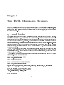
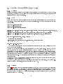
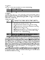
Figure 1.1: Sample simulation of a negatively autoregulated transcriptional circuit.
simulationTime = 14*60*60;
tic
[simData] = txtl_runsim(Mobj,simulationTime);
toc
t_ode = simData.Time;
x_ode = simData.Data;
% Plot the results
txtl_plot(t_ode,x_ode,Mobj);
Figure 1.1 shows the output from this code (plotted using the txtl_plot function).
4
Chapter 2
Installation
2.1 Prerequisites
Our toolbox builds upon basic MATLABTM functionality and the Simbiology toolbox. Therefore the presence
of Simbiology is essential for our TXTL toolbox to work. The toolbox was tested on MATLAB 2012 for Mac
OSX, MATLAB 2010a for Linux and MATLAB 2011b-2012a for Windows.
2.2 Installing the toolbox
1. Download the toolbox zip archive txtl_0_42a.tgz from the project's SourceForgeTM page: http://
sourceforge.net/p/txtl/wiki/Home/
2. Unzip the le into a directory of your choice. In windows, this may take two unzip steps. Ultimately,
you should have a folder named txtl_0_42a.
3. Set the MATLAB working directory to the folder txtl_0_42a, or a parent folder.
4. You may either run
txtl_init
beginning of each MATLAB session or add the directories there to the search path and save.
5. All done. Try opening and running negautoreg.m in the Examples directory. If this runs without error,
you have successfully installed the TXTL modelling toolbox. Congrats!
5
Chapter 3
Examples
3.1 Gene Expression with Fluorescent Reporter (geneexpr)
3.1.1 Overview
This example shows constitutive expression of the destabilized enhanced Green Fluorescent Protein (deGFP)
from a gene on a plasmid. It shows one of the simplest circuits that can be modelled with the modelling
toolbox, and in doing so, illustrates its basic features. These include displaying the evolution of the expressed
protein (deGFP) levels, resource usage (Amino Acids (AA) and Nucleotide Pairs (NTPs)), the evolution of
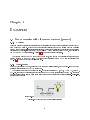
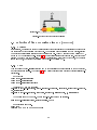
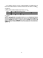
the DNA and mRNA concentrations. Figure 3.1 shows a schematic of this circuit.
The diagram shows the DNA made of the p70 promoter, the most common constitutive promoter in the
toolbox, followed by the deGFP gene. The gene is then transcribed into mRNA which is translated into
DNA. 3.2 shows the output plot for this example.
3.1.2 Walk-through
If you have not already done so, ensure that you are in the \trunk directory, and run txtl_init to add the
necessary directories to the MATLAB search path.
The rst step is to decide on a extract to use. The extract contains RNAP, Ribo, σ28 and σ70, RecBCD,
RNA-ase, and sets up the reactions for the formation of RNAP70 and sequestration of RecBCD. The extract
we will be using will be created using parameters dened in the external conguration le 'E15_cong.csv',
and is implemented as:
schematic.png
Figure 3.1: Schematic of the gene expression circuit'
6
tube1 = txtl_extract('E15');
Note that this command returns a handle to a Simbiology model object. This is stored in the aptly named
variable tube1. We will later combine the 'contents' of this tube with those of other tubes, just like we do in
the experimental protocol. One may read about Simbiology model objects at http://www.mathworks.com/
help/simbio/ug/what-is-a-model.html#bsrhh1k and http://www.mathworks.com/help/simbio/ref/modelobject.
html.
Next, we dene the buer (containing AA and NTP) to use, and store it in tube2. Once again, the buer
contents are drawn from the conguration le 'E15_cong.csv':
tube2 = txtl_buffer('E15');
We then use the txtl_newtube command to create a new model object which will contain the DNA we
wish to use. This is done as follows:
tube3 = txtl_newtube('gene_expression');
The next step is to dene the DNA sequences to be added to tube3. This is done using the txtl_add_dna
command:
dna_deGFP = txtl_add_dna(tube3, 'p70(50)', 'rbs(20)', 'deGFP(1000)', 1, 'plasmid');
Refer to the description of the txtl_add_dna command in Ÿ3.2 for full details of its usage. For our purposes,
it suces to know that this DNA is loaded onto a plasmid, and contains a p70 promoter (constitutive, 50
base pairs (BP) in length), a 20BP RBS domain, and a 1000BP deGFP gene. Furthermore, the DNA is such
that the nal concentration of this DNA in the combined tube will be 4nM.
We then simply combine the extract, buer, and DNA:
Mobj = txtl_combine([tube1, tube2, tube3]);
We now have to set the amount of time we want our simulation to run for and calling the txtl_runsim
command as follows:
[simData] = txtl_runsim(Mobj,14*60*60);
t_ode = simData.Time; x_ode = simData.Data;
This call to txtl_runsim takes the Simbiology model object and the experiment duration to be simulated,
and runs the simulation from time zero to time 14 hours. It returns a simData object, from which we
can extract a vector of time points in that range (t_ode) and a matrix x_ode, where each column is the
concentrations of a species in the model at time points corresponding to t_ode. For more information, please
refer to Chapter 3: Overview of the Core Processes.
Finally, the modelling toolbox contains a set of plotting tools that simplify the plotting of standard
species, like Proteins, DNA, RNA and resources. We use txtl_plot to accomplish this. One may simply
call txtl_plot with the data and model object as follows:
txtl_plot(t_ode,x_ode,Mobj);
leading to a default set of species to be plotted.
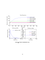
3.1.3 Results
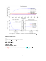
Figure 3.2 shows the output of the plotting command for this example. The top plot shows the protein
species present in the model, the bottom left plot shows the DNA and mRNAs in the system, and the
bottom right plot displays the resource usage. We observe that deGFP almost entirely exists in the mature
state, and rises constantly for the rst 200 minutes, before reaching a steady state of about 2uM.
7
Figure 3.2: Gene Expression Output
8
3.2 Negative Autoregulation (negautoreg)
3.2.1 Overview
Negative autoregulation refers to the repression of gene expression by a protein encoded by that very gene.
In this code, we will show that dimerized tetR protein represses its own production, and thus leads to a
relatively low steady state concentration.
3.2.2 Code
Please work through the Gene Expression example above to get basic familiarity with the commands and
their usage. This example is slightly more complex than geneexpr. We provide the entire code for this
example below:
tube1 = txtl_extract('E9');
tube2 = txtl_buffer('E9');
tube3 = txtl_newtube('negautoreg');
dna_tetR = txtl_add_dna(tube3, 'thio-junk(500)-ptet(50)', 'rbs(20)', 'tetR(647)-lva(40)', 16,
'linear');
dna_deGFP = txtl_add_dna(tube3, 'p70(50)', 'rbs(20)', 'deGFP(1000)', 16, 'linear');
dna_gamS = txtl_add_dna(tube3, 'p70(50)', 'rbs(20)', 'gamS(1000)', 1, 'plasmid');
Mobj = txtl_combine([tube1, tube2, tube3]);
simulationTime = 8*60*60;
[t_ode, x_ode, mObj, simData] = txtl_runsim(Mobj, simulationTime);
txtl_plot(t_ode,x_ode,Mobj);
The important dierences from the gene expression examples are that here we add 3 pieces of DNA into
tube 3, two of which are linear.
The tetR DNA uses a ptet promoter, which is repressed by the tetR protein dimer. Attached to the ptet
promoter, there are two domains (thiosulfate 'thio' and junk DNA 'junk) which lower the rate of DNA
degradation by the exonuclease RecBCD. The tetR DNA also shows an 'lva' tag, which attaches a amino
acid sequence to the tetR protein and marks it for degradation by the protease ClpXP. In a futire version,
all the 'lva' tags will be replaced by the 'ssrA' tags, although for the functioning of this toolbox, this name
change is inconsequential. The reaction rate parameters for ClpXP's action are currently in the process of
being determined.
The second DNA, deGFP, is just like in the gene expression exampe, except that in this case it is mounted
on a 'linear' DNA, and therefore can be degraded.
The third DNA, gamS, is mounted onto a plasmid, and is thus safe from degradation. GamS helps to sequester the RecBCD exonuclease, providing protection tot the DNA.
3.2.3 Results
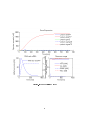
Figure 3.3 illustrates a number of features: expression of gamS, tetR and the tetR dimer, the respective
mRNAs, and resources. The rst thing to note is that expression levels in this example are an order of
magnitude lower than in gene expression. There are two reasons for this: The use of 'linear' DNA, which
means that RecBCD mediated DNA degradation is active, and the quick depletion of the RNA, due to the
greater amount of RNA produced.
9
Figure 3.3: Negative Autoregulation Output
10
schematic.png
Figure 3.4: Schematic of the induction circuit'
3.3 Induction of Gene Expression using aTc (induction)
3.3.1 Overview
In this circuit, we explore the eect of varying levels of the inducer 'aTc' on the expression of a gene under
the control of the tetR repressed ptet promoter. The expressed gene is precisely the tetR protein, leading
to a negative autoregulation circuit as in the previous example. This DNA is loaded onto a plasmid DNA,
and so no DNA degradation occurs. Figure 3.4 shows the circuit diagram for this example. Note that in the
diagram, the deGFP and tetR are fused, while in the simulation, we only use the tetR gene, but we set its
length to be 1200, comparable to the length of the tetR-deGFP fusion DNA.
3.3.2 Code
This code uses the txtl_addspecies command to add increasing amounts of 'aTc' to the model object,
and executes the simulation. The Figure 3.5 below plots the levels of tetR protein at dierent 'aTc' concentrations.
Set up tubes:
tube1 = txtl_extract('E6');
tube2 = txtl_buffer('E6');
tube3 = txtl_newtube('circuit');
Construct DNA and add to tube3:
dna_tetR = txtl_add_dna(tube3, 'thio-junk(500)-ptet(50)', 'rbs(20)', 'tetR(1200)-lva(40)',
16, 'plasmid');
dna_gamS = txtl_add_dna(tube3, 'p70(50)', 'rbs(20)', 'gamS(1000)', 0, 'plasmid');
Add protein gamS to the model. We used txtl_add_dna to set up its reactions.
gamS = txtl_addspecies(tube3, 'protein gamS', 100);
Dene levels of aTc to use.
count = 1;
levels = [0 2 5 10 20 40 100 300 1000];
11
colors = {'r', 'b', 'g', 'c', 'm', 'y', 'k', 'r', 'b'};
Combine tubes:
Mobj = txtl_combine([tube1, tube2, tube3]);
Iteratively Simulate the model with dierent levels of aTc.
for atc = levels
configsetObj = getconfigset(Mobj, 'active');
set(configsetObj, 'StopTime', 6*60*60);
[t_ode, x_ode, Mobj, simData] = txtl_runsim(Mobj, configsetObj);
figure(2); hold on;
itetR = findspecies(Mobj, 'protein tetR');
plot(t_ode, x_ode(:, itetR), colors{count});
labelscount = [int2str(atc) ' nM aTc'];
if count < size(levels,2)
inducer = txtl_addspecies(Mobj, 'aTc', levels(count+1)-levels(count));
count = count + 1;
end
end
title('Time Responses');
lgh = legend(labels, 'Location', 'Northwest');
legend(lgh, 'boxoff');
ylabel('Species amounts [nM]');
xlabel('Time [min]');
3.3.3 Results
Figure 3.5 shows the concentrations of tetR. Note that this is not the standard plot generated in the previous two examples. We used the findspecies function to obtain the index of the species to plot ([protein
tetR]) by using that index to access the relevant column of the data vector x_ode.
We note that as the aTc concentration is increased, the level of tetR in the system increases due to
reduced repression of ptet by protein tetRdimer.
12
Figure 3.5: Induction of tetR expression due to aTc
13
Chapter 4
Core Functionalities
4.1 User Commands
Here we give details about the various functions you will be using in the modelling toolbox.
txtl_extract
Set up a tube containing the TXTL 'Extract'. This is usually the rst function to be called, and sets up
various basic reaction rates, species and reactions. It takes the name of a conguration le containing parameter values as an input and returns a pointer to a Simbiology model object.
The syntax and the usage of this function are summarized below, along with the species, reactions, parameters, and initial concentrations the function sets up:
tube = txtl_extract(name)
Syntax
Input
name: (string) name of extract
Output
tube: pointer to Simbiology model object
Usage
tube1 = txtl_extract('E6');
Species
RNAP, Ribo, σ28 and σ70, RecBCD, RNA-ase
Reactions
Formation of RNAP70 and sequestration of RecBCD
Parameters
Set-up reaction rates, AA and NTP models, and initial amounts dened in the
txtl_reaction_config class. See txtl_reaction_config in Ÿ3.3 for more information. This function also sets-up the initial amounts for Ribosomes, RNAP, σ28
and σ70. Their values can be found in the le, including the references they were
extracted from.
txtl_buffer
Set up a tube containing the TXTL 'Buer'. This sets up the NTP and AA species, with initial concentrations from the supplied conguration le (same as the one used for the 'Extract').
Syntax
Input
Output
Usage
Species
tube = txtl_buffer(name)
name: (string) name of buer.
tube: pointer to Simbiology model object
tube2 = txtl_buffer('E6');
NTP and AA
14
txtl_newtube
Create a new model object ('tube') containing one compartment called 'contents').
Syntax
Input
Output
Usage
tube = txtl_newtube(name)
name: (string) name of new tube.
tube: pointer to Simbiology model object
tube3 = txtl_newtube('circuit');
txtl_add_dna
This function creates a piece of DNA that the user species, and sets up all the associated species and
reaction objects, initial concentrations, and reaction rate parameters. The tube the DNA is placed in, the
initial amount, and the type of DNA, 'linear' or 'plasmid', are specied by the user. The function returns a
pointer to the DNA species object.
This is summarized below:
dna = txtl_add_dna(tube, prom_spec, rbs_spec, gene_spec, dna_amount,
Syntax
type)
Input
• tube: pointer to the model object to add the DNA to.
• prom_spec: (string) string representing promoter. See below for details.
• rbs_spec: (string) ribosome binding site with optional length in Base Pairs.
• gene_spec: (string) gene string. See below.
• dna_amount: (double) amount of DNA to be added, in nM. This will be the
nal concentration in the experiment after the tubes have been combined.
• type: (string) type of DNA: 'linear' or 'plasmid'.
Output
Usage
dna: pointer to DNA object.
dna_tetR = txtl_add_dna(tube3, 'thio-junk(500)-ptet(50)', 'rbs(20)',
'tetR(647)-lva(40)-terminator(100)', 16, 'linear');
The prom_spec is a string containing the name of the promoter to be used (this is a necessary argument,
and needs the corresponding promoter le to be present in the MATLAB search path), with an optional length
in base pairs. If the length is not specied, the default length specied in a txtl_param_<promoterName>.csv
le is used. There are two other optional strings that can be specied: a 'thio' and a 'junk(n)', where n
is an optional integer value. The 'thio' string tells the Toolbox that a thiosulfate group is present , and this
confers protection to the DNA from degradation. As of this release, the amount of protection is arbitrarily
set, and will be corrected once the relevant experiments and system ID are carried out. Similarly, junk DNA
slows down the DNA degradation rate by an amount proportional to the length of this DNA added, with the
constant of proportionality to be determined. As an example, a full specication of this string would look
like: 'thio-junk(500)-ptet(50)'. Note that only 'linear' DNA can be degraded. 'plasmid' DNA does not
degrade in this toolbox.
The gene_spec string works similarly to the prom_spec string. The name of the gene is required, and
this must be associated with an existing protein le. Defaults work similarly as in prom_spec, with a
required component conguration le. The optional strings are: 'ssrA(n)' and 'terminator(n)', where ssRA
is a degradation tag (length n) which marks the protein for degradation, and the terminator will have
capabilities in future releases of the toolbox.
15
Note: Generally, the lengths in BP are used to calculate transcription and translation rates. These
lengths will have greater prevalence in the calculation of reaction rates in future versions of the toolbox.
txtl_combine
Combine the contents (species and reactions) of tubes to form a new tube.
Syntax
Input
Output
Usage
Mobj = txtl_combine(tubelist, vollist)
tubelist (vector of pointers) A list of tubes to combine together.
Mobj: pointer to the new tube.
Mobj = txtl_combine([tube1, tube2, tube3]
txtl_runsim
Simulate model. txtl_runsim is the main function to execute the MATLAB dierential equation solvers to
solve for the species concentration trajectories forward in time from a specied initial condition. It returns
a vector array t_ode_output containing time points and a matrix array x_ode_output containing the corresponding species concentration values. x_ode_output is arranged such that each column corresponds to a
species, and contains that species' concentrations at the time points corresponding to the points specied in
t_ode_output.
16
Syntax
Input
[simData] = txtl_runsim(modelObj, simulationTime)
with the following variations:
Input:
(Mobj)
(Mobj ,simulationTime)
(Mobj ,simulationTime, simData)
(Mobj ,simulationTime, t_ode, x_ode)
Output:
[simData]
[t_ode, x_ode]
[t_ode, x_ode, Mobj]
[t_ode, x_ode, Mobj, simData]
• modelObj: pointer to the model object to simulate. This is the Simbiology
model object returned by txtl_combine.
• t_ode: optional vector array containing time point data from previous runs.
See below for more information.
• x_ode: optional matrix array containing species concentration trajectory data A
from previous runs. See below for more information.
• simData: optional structure containing simulation data, such as names of species
and previous simulation data.
Output
• t_ode_output: vector array containing time point data from this run, appended
to data from previous runs, if any.
• x_ode_output: matrix array containing species concentration trajectory data
from this run, appended to data from previous runs, if any.
• Mobj: model object the simulation was run on.
• simData_output: optional structure containing simulation data, such as names
of species.
Usage
[t_ode, x_ode, Mobj, simData] = txtl_runsim(Mobj, simulationTime,
t_ode, x_ode);
useful feature of txtl_runsim is that is allows one to 'continue' a simulation from the end point of a previous
run, with new species of more of existing species added before the simulation is continued. This models the
situation when additional reagents like inducers or proteins are added to an experimental preparation after
the experiment has commenced. This can be done as follows:
First call to txt_runsim
[t_ode, x_ode, Mobj, simData] = txtl_runsim(Mobj, simulationTime);
Execute other code, say, add some inducer:
aTc = txtl_addspecies(mObj, 'aTc', 50);
Continue simulation:
[t_ode2, x_ode2, Mobj, simData] = txtl_runsim(Mobj, t_ode, x_ode, simData);
17
The new arrays t_ode2, x_ode2 contain the results of the rst simulation appended to the results of
the second simulation. Thus, one can simply plot these to view the results since the beginning of the rst
simulation.
txtl_plot
Plotting command that simplies the plotting of the evolution of the concentrations of the standard species:
Proteins of interest, Resources, and DNA and RNA concentrations.
Syntax
Input
txtl_plot(t_ode, x_ode, Mobj);
or
txtl_plot(t_ode, x_ode, Mobj, dataGroups);
• t_ode: vector array containing time point data.
• x_ode: matrix array, with each column containing data corresponding to
the time evolution of the concentration of once species in the model. See
txtl_runsim for more details.
• Mobj: pointer to the model object associated with the data to be plotted.
• dataGroups: these are optional cell arrays of strings which enable the user to
customize what is plotted. We will provide documentation on these in a future
version of this manual.
Usage
txtl_plot(t_ode, x_ode, Mobj);
where t_ode, x_ode and Mobj are the variables dened in the le.
txtl_addspecies
txtl_addspecies allows the addition of any species directly to the model object. If this species is already present in the model, the function simply increases its concentration by the amount that is added.
If the species is a protein and is not present in the model, then txtl_addspecies adds the protein, and
sets up all the associated species (dimers, complexes) and reactions (repression, induction, degradation, etc.).
Syntax
Input
simBioSpecies = txtl_addspecies(tube, name, amount)
• tube: pointer to the model object to add the species to.
• name: (string) name of the species to be added. See below for format of string.
• amount: (double) amount, in nM, of the species to add or to increase existing
species' concentration by.
Output
Usage
simBioSpecies: pointer to the species object just added.
inducer = txtl_addspecies(Mobj, 'aTc', 20);
Note that name strings have the following format:
18
Standard
species
Expressed
proteins
'<name of specie>'
Examples: 'aTc', 'IPTG', 'ClpXP'
'protein <name of protein>'
Examples: 'protein tetR', 'protein lacI'
txtl_findspecies
txtl_findspecies is a useful function to nd the column index of a given species in the matrix data array
(x_ode) returned by txtl_runsim. This enables the user to access the trajectory of any species in the model.
Syntax
Input
indexlist = findspecies(Mobj, namelist)
• Mobj: pointer to the model object get species indices from.
• namelist: (string or cell array) name of the species to be searched for, or a cell
array of such strings.
Output
Usage
indexlist: (integer or vector of integers) index of the species in the list of species in
the model object, and in the data array x_ode returned by txtl_runsim. The vector
is returned when namelist is a cell array, and the entries of the vector correspond to
the indices for the entires in namelist.
iGFP = findspecies(Mobj, 'protein deGFP*');
iRNAP28_DNA_complex = findspecies(Mobj,'RNAP28:DNA
p28_ptet--rbs--deGFP')
We can use the output of this function to plot the trajectory of the species as follows:
iGFP = findspecies(Mobj, 'protein deGFP*');
plot(t_ode, x_ode(:, iGFP));
or use the index directly:
plot(t_ode_,x_ode(:,findspecies(Mobj,'DNA p28_ptet--rbs--deGFP:protein tetRdimer')),'r')
Note: one can see a list of all the species in the model by running the command speciesNames =
get(Mobj.species, 'name'), where Mobj is the model object.
19
Chapter 5
Appendix
5.1 Externally Specied Parameters
txtl_reaction_cong (class)
The txtl_reaction_cong class enables users to input custom reaction parameters for the TXTL extract into
their model. This is done via a comma-separated-value (.csv) le. The parameters controlled by this class
are given in the properties of this class.
List of Parameters
1. NTPmodel: There are two models for transcription that the toolbox can switch between, model 1 and
2. We recommend keeping this setting at model 2, since model 1 suers from stiness of the dierential
equations to be solved, and is primarily used for testing purposes.
2. AAmodel: Similar to NTPmodel above, we recommend keeping this setting at 2.
3. Transcription_Rate:
NTP : RNAP70 : DNA → DNA + RNA + RNAP
(5.1)
(5.2)
This is the reaction for transcription, with transcription rate calculated as:
Transcription_Rate =
(log(2) × 50)
RN A_length
(5.3)
(5.4)
and a dummy reaction for NTP consumption, with rate Transcription_Rate_dummy
NTP : RNAP70 : DNA → DNA + RNAP
RN A_length
Transcription_Rate_dummy =
− 1 × Transcription_Rate
100
20
(5.5)
(5.6)
4. Translation_Rate: Reaction rate for:
ATP : AA : Ribo : RNA → Protein + RNA + Ribo
(5.7)
(5.8)
This is the reaction for translation, with reaction rate calculated as:
Translation_Rate =
(log(2) × 0.64)
protein_length
(5.9)
(5.10)
and a dummy reaction for AA consumption, with rate Translation_Rate_dummy
ATP : AA : Ribo : RNA → RNA + Ribo + ATP
protien_length
Translation_Rate_dummy =
− 1 × Translation_Rate
100
(5.11)
(5.12)
5. DNA_RecBCD_Forward and DNA_RecBCD_Reverse: Complex formation and dissociation
rate between RecBCD enzyme and DNA.
DNA + RecBCD DNA : RecBCD
(5.13)
6. DNA_RecBCD_complex_deg: Degradation rate of RecBCD-DNA complex.
DNA : RecBCD → RecBCD
(5.14)
7. Protein_ClpXP_Forward and Protein_ClpXP_Reverse:
Complex formation and dissociation rate between ClpXP enzyme and a protein tagged for degradation.
Protein + ClpXP Protein : ClpXP
(5.15)
8. Protein_ClpXP_complex_deg Degradation rate of ClpXP-Protein complex.
Protein : ClpXP → ClpXP
(5.16)
9. RNAP_S70_F and RNAP_S70_R: RNAP70 formation and dissociation rate.
RNAP + σ 70 RNAP70
(5.17)
10. AA_Forward and AA_Reverse: Binding and dissociation of AA to Ribosome mRNA complex:
AA + Ribo : RNA AA : Ribo : RNA
(5.18)
11. Ribosome_Binding_F and Ribosome_Binding_R: Binding and dissociation rated fro RNARibosome complex:
Ribo + RNA Ribo : RNA
(5.19)
RNA + RNAase → RNAase
(5.20)
12. RNA_deg: RNA degradation rate:
13. NTP_Forward and NTP_Reverse: Binding and dissociation of NTP to the RNAP70-DNA complex:
NTP + RNAP70 : DNA NTP : RNAP70 : DNA
21
(5.21)
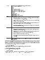
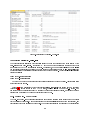
Figure 5.1: Screenshot of le 'E6_cong.csv'
Conguration le: 'E<n>_cong.csv'
The conguration le associated with this class is used to dene the contents of the tubes created by the
txtl_extract and txtl_buffer. the integer <n> in the name of the le refers to the label of the buer
and extract in the TXTL experimental protocol. For instance, if we use extract 'E6' and buer 'B6' in
the experimental protocol for a circuit, we would create a conguration le named 'E6_cong.csv', which
would encapsulate the variations between batches of the buer and extract. We use this le in the modelling
toolbox as follows:
tube1 = txtl_extract('E6');
tube2 = txtl_buffer('E6');
Note that we do not dene two separate conguration les for the buer and extract. All the information
needed is stored in one le.
Figure 5.1 shows a screenshot of the conguration le 'E6_cong.csv'. This le is a 'Comma Separated
Value' le, and is best opened in the MATLAB editor, with the 'File > Open as Text...' option. One
can create custom conguration les by modifying the parameter values in this le, and saving it under a
dierent name according to the naming convention dened above.
txtl_component_cong (class)
The txtl_component_cong class enables users to input custom reaction parameters for the components
they are using in their model. Components are found in the components directory in the main directory, and
contain les that dene proteins and promoters. The parameters present in the class and the corresponding
22
conguration les are dependent on the components being used, but are highly analogous to the previous
section. Editing of the conguration les is also carried out as above.
5.2 List of Core Reactions
These reactions are currently those of Dan, and refer to the Toxin-Antitoxin System. We will modify them
so that they correspond to the reactions in the TXTL toolbox.
5.2.1 Basic
RNAP + σ 70 RNAP70
(5.22)
RNAP → φ
(5.23)
RNAP
70
→σ
(5.24)
70
ATP → ADP
(5.25)
RecBCD + GamS RecBCD : GamS
(5.26)
5.2.2 Transcription
(5.27)
DNA + RNAP70 RNAP70 : DNA
70
70
RNAP : DNA + NTP NTP : RNAP : DNA
70
70
NTP : RNAP : DNA → DNA + RNA + RNAP
(5.28)
(5.29)
Dummy reaction for NTP consumption, see previous section for rates:
NTP : RNAP70 : DNA → DNA + RNAP70
(5.30)
5.2.3 Translation
RNA + Ribo Ribo : RNA
(5.31)
Ribo : RNA + AA + ATP AA : ATP : Ribo : RNA
(5.32)
AA : ATP : Ribo : RNA → RNA + protein + Ribo
(5.33)
Dummy reaction for AA consumption, see previous section for rates:
AA : ATP : Ribo : RNA → RNA + Ribo
(5.34)
5.2.4 Protein Degradation (if tagged)
(5.35)
ClpX → ClpX∗
protein + ClpX∗ protein : ClpX∗
∗
∗
protein : ClpX + ATP → ClpX
(5.36)
(5.37)
(5.38)
∗
ClpX → φ
23
5.2.5 Protein reactions
Multimerization
protein + protein protein_dimer
(5.39)
protein_dimer + protein_dimer protein_tetramer
(5.40)
Repression
Here the DNA has a promoter which is repressed by protein A. For example, tetR_dimer can repress
ptetrbsgene.
protein_A + DNA_A DNA_A : protein_A
(5.41)
Notice that in the transcription step, there is no reaction for RNA polymerase binding to the protein-bound
DNA, hence repression.
Maturation
A few proteins, like ClpX and deGF P , undergo maturation.
protein → protein∗
(5.42)
5.2.6 Other Degradation
DNA + RecBCD DNA : RecBCD
(5.43)
DNA : RecBCD → RecBCD
(5.44)
RNA + RNase RNA : RNase
(5.45)
RNA : RNase → RNase
(5.46)
Ribo : RNA + RNase Ribo : RNA : RNase
(5.47)
Ribo : RNA : RNase → RNase + Ribo
(5.48)
AA : ATP : Ribo : RNA + RNase AA : ATP : Ribo : RNA : RNase
(5.49)
AA : ATP : Ribo : RNA : RNase → RNase + AA + ATP + Ribo
(5.50)
24