1
Adaptive Optics simulation IDL code
A User Manual
Fran
cois Rigaut
March 21, 2001
Contents
1 Introduction
3
2 The input les
5
2.1
2.2
2.3
2.4
2.5
ao.par . . . . . . . . . . . .
Dimensioning the system . .
sensor.par . . . . . . . . . .
mirror.par . . . . . . . . . .
The phase screens . . . . .
..
..
..
..
..
..
..
..
..
..
.
.
.
.
.
..
..
..
..
..
..
..
..
..
..
..
..
..
..
..
.
.
.
.
.
..
..
..
..
..
..
..
..
..
..
..
..
..
..
..
.
.
.
.
.
..
..
..
..
..
..
..
..
..
..
..
..
..
..
..
.
.
.
.
.
..
..
..
..
..
..
..
..
..
..
..
..
..
..
..
.
.
.
.
.
..
..
..
..
..
..
..
..
..
..
..
..
..
..
..
3 The Main Routines
3.1
3.2
3.3
3.4
init . . . . .
dointer . . .
mkmatcom
loop . . . .
..
..
..
..
..
..
..
..
5
12
13
13
14
15
..
..
..
..
.
.
.
.
..
..
..
..
..
..
..
..
..
..
..
..
.
.
.
.
..
..
..
..
..
..
..
..
..
..
..
..
4 Running simul
.
.
.
.
..
..
..
..
..
..
..
..
..
..
..
..
.
.
.
.
..
..
..
..
..
..
..
..
..
..
..
..
.
.
.
.
..
..
..
..
..
..
..
..
..
..
..
..
.
.
.
.
..
..
..
..
..
..
..
..
..
..
..
..
15
15
16
16
17
4.1 X form interface to simul . . . . . . . . . . . . . . . . . . . . . . . . . . . . . . . . . . . . . . . . 17
4.2 Running Simul from the command line . . . . . . . . . . . . . . . . . . . . . . . . . . . . . . . . . 18
4.3 Running time considerations . . . . . . . . . . . . . . . . . . . . . . . . . . . . . . . . . . . . . . . 20
5 The output les
23
A Batch Examples
25
1
2
CONTENTS
Chapter 1
Introduction
This code is written exclusively in IDL (Interactive Data Language) language. It should be executed in the IDL
environment.
This code is intended to simulate adaptive optics systems featuring curvature wavefront sensors (CWFS)
or Shack-Hartmann wavefront sensors (SHWFS), in combination with piezostack (PZT) or bimorph mirrors
(BIM). The code is organized into subroutines that allow to take interaction matrices, invert them, and run a
dynamic close-loop simulation (that includes the temporal behavior of the loop).
The whole thing was developed by myself in an approximately 6 months period. Later I added subroutines
and a GUI. Version 4.2 and 4.3 were developped in the mist of 1997-1999. I estimate the full developement time
to something around 12 man month, mostly when I was at CFHT. It was initially developed to investigate the
performance of the PUEO system (19 subapertures curvature system on the Canada{France{Hawaii Telescope
located atop Mauna Kea in the big island of Hawaii). I must warn the potential user that it is not bulletproof
and certainly not bug free. However, IDL is kind with us, and most of the time will crash gracefully and
allow and easy tracing of the error. I try to follow and solve bugs. If you nd one, please let me know at
[email protected].
The les required to run the code are listed below. More detailled descriptions can be found in the next
section. Some of the les are mandatory, some other are optionnal (the program check if they are in the current
directory, and read them out in this case). Some les may be also required to dene the system geometry in
the case of a non-square subapertures/actuator pattern.
Mandatory les :
simul.pro
File that contains the main IDL procedure, simul, plus a bunch of other subroutines. This le
has to be somewhere into the IDL_PATH, in order for IDL to nd it. It has to be compiled when
entering IDL by typing
.run simul
ao.par
Phase screen(s)
This is the main parameter le. It contains the parameter defaults. To change it, you can
either edit it manually or use the editor provided in the simul GUI.
Phase screen(s) used to simulate atmospheric turbulence (e.g. cscreen128_10.fits). Those
are ts les. See below (section 2.5) for an explanation of how they are normalized, their format,
etc...
Optionnal les :
sensor.par
This is the sensor parameter le for radial congurations. SHWFS dened on a square geometry
do not use this le. Used exclusively for curvature sensors in the current version.
3
4
CHAPTER 1. INTRODUCTION
mirror.par
wfs stat ab.par
sort modes.par
This is the mirror parameter le for radial congurations. PZT mirrors dened on a square
geometry do not use this le. Used exclusively for bimorph mirrors in the current version.
This le contains the zernike coeÆcient of the WFS path phase aberrations.
This le allow to sort the modes found by the modal decomposition in a given order.
The following is a list of output les, written by simul .
This is the journal le into which every operation executed by simul is dumped. For each
\operation" (matrix acquisition, inversion, initialization, loop run) it contains the state of the
system and the results of the operation. Ascii and editable.
sensor.fits Fits le of the sensor conguration. Just for information.
pupil.fits Image of the pupil. For information only.
Influence functions in the form pzt\_s**\_p**\_**.fits for the piezostack mirrors, where the ** are the size
of the array (e.g 128 if 128128 are used), the diameter of the pupi in pixel and the number
of actuators respectively, and in the form bim\_s**\_p**\_e**.fits where the ** are the
size of the array (e.g 128 if 128128 are used), the diameter of the pupi in pixel and the
number of electrodes respectively. Those inuence fonctions are saved in order to be used for
subsequent use of simul in the same conguration. This le is written at the complexion of
the initialization.
mats.fits Fits le that contains the interaction matrix and the command matrix. This le is written at
the complexion of the command matrix computation routine.
mta.fits Transformation matrix modes to actuators/electrodes. Written only if modal inversion is required.
simul.avimage Beware, this is a ts le. It contains the average compensated image over the whole loop run.
Written at the complexion of the loop procedure.
modevar.dat Ascii le. Contains the mode variance in a loop run. Written at the complexion of a loop run.
The parameter ao.sim.calcmode has to be set for this le to be written.
cb mes The cb\_** are what is called \circular buer", for historical reason. Here, they have nothing
of circular nature. This one contains the measurement. One line written at each iteration of
the loop run. ao.sim.cb_output has to be set for this le to be written.
cb com As cb\_mes, except it contains the mirror commands.
cb modc As cb\_mes, except it contains the mode coeÆcient of the modal decompositon of the input
(turbulent) phase.
cb modc As cb\_mes, except it contains the mode coeÆcient of the modal decompositon of the output
(compensated) phase.
simul.res
Chapter 2
The input les
This section gives more details on the content of the parameter les.
2.1
ao.par
This le contains the default parameters to be used in the code. It is read out when simul is started.
can also read other par les by using the keyword parfile, i.e. :
simul
IDL> simul,/x,parfile='ao.par.my_config.cwfs19'
All the parameters defaults can be changed to accomodate user requirements. This le is formatted so that
IDL can read easily its content as an IDL structure. It is in fact made of 9 IDL structures that are later gathered
into one large IDL structure called ao. The 8 IDL individual structures are substructures of ao, namelly :
ao.zim
ao.mir
ao.wfs
ao.gs
ao.ttgswfs
ao.tel
ao.loop
ao.atm
ao.isop
ao.sim
Interaction matrix parameters
Mirror parameters
WFS parameters
Guide Star parameters
Tip-Tilt guide star and WFS parameters
Telescope parameters
Close-loop parameters
Atmosphere parameters
Isoplanatism related parameters
Simulation parameters
It is very easy to list or modify each substructure elements when into IDL. These elements can be addressed
by the name of the structure dot the name of the substructure dot the name of the element. For instance, one
can address the mirror type by the name ao.mir.type. So one can modify parameters on the IDL command
line by typing simply, for instance :
ao.mir.type = 'piezostack'
ao.gs.starmag = 14.5
ao.loop.it_time = 0.01
and so on. This is convenient for command line batches.
Here is an example of a parameter le :
; File written on Wed Mar 21 11:18:45 HST 2001
; Parameter file for simul.pro, Version 4.3 and later
5
6
CHAPTER 2. THE INPUT FILES
; INTERACTION MATRIX ACQUISITION AND INVERSION
{zim,
v_dm
: 0.500000,
; Voltages on the DM to record interaction matrix
v_tt
: 0.500000,
; Voltages on the TT to record interaction matrix
inversion
: 'zonal',
; Method of inversion, 'modal' or 'zonal'
mta
: '',
; Conversion matrix mode -> actuators
mode_enable
: '',
; Mode enable/disable for modal inversion
forcenev
: 1,
; # of eigenval. to force to Zero in the inversion
cond_number
: 0.0100000,
; conditioning number of matrix to invert
matrices
: 'mats.fits'}
; File to read interaction and command matrices fr
; MIRROR
{mir,
type
parfile
def_file
tt
v_limit
hyst : 0.00000,
nxact
:
:
:
:
:
'bimorph',
'mirror.par',
'bim_s64_p60_e19.fits',
0,
6000.00,
: 50}
; SENSOR
{wfs,
type
: 'curvature',
geom
: 'radial',
parfile
: 'sensor.par',
lambda
: 7.00000e-07,
; SHWFS only parameters :
nxsub
: 7,
pixsize
: 0.262033,
subsize
: 2.09626,
rnoise
: 0,
blur
: 0,
threshold
: 0.00000,
; CWFS only parameters :
l
: 0.150000,
sinus
: 0,
fieldstop
: 3.00000,
gainrav
: 1.00000,
mask
: 0.300000}
; GUIDE STAR
{gs,
noise
lgs
altitude
thickness
laser_2w0
lauch_diam
lauch_pos
lauch_ttm
lauch_ttm_gain
extended
gsmap
gsmapscale
starmag
skymag
zeropoint
:
:
:
:
:
:
:
:
:
:
:
:
:
:
:
1,
0,
95000.0,
8000.00,
0.300000,
0.450000,
0.00000,
0,
-0.800000,
0,
'extended3.fits',
0.0500000,
8.00000,
20.3000,
2.00000e+10}
; TIP-TILT GUIDE STAR AND SENSING
{ttgswfs,
ttgs
: 0,
starmag
: 10.0000,
skymag
: 20.7000,
psize
: 0.257022,
fov
: 1.02809,
lambda
: 7.00000e-07,
threshold
: -1.00000,
gain
: 0.0100000,
noise
: 0.00000}
;
;
;
;
;
'bimorph' or 'piezostack' or 'zernike' or 'tip-t
mirror par file (for radial config only)
file that contains the influence functions
Is there a tip-tilt mirror (0/1) ?
Maximum voltage on the electrodes
; deformable mirror hysteresis
; linear number of actuator (piezostack only)
;
;
;
;
'curvature' or 'hartmann'
WFS geometry : 'radial' or 'square'
Sensor par file (radial config only)
WFS wavelength (in meter)
;
;
;
;
;
;
;
Linear number of subaperture (SHWFS only)
Pixel size in arcsec (SHWFS only)
subaperture size in arcsec (SHWFS only)
e- rms read noise (SHWFS only)
Blur image to avoid discretization noise (SHWFS
Threshold on SHWFS in count if positive,
in percent if negative (e.g. -0.5 = 50%) and no threshold if -1
;
;
;
;
;
Extra-focal distance in m (CWFS only)
# of point in a 1/4 wave of mm scanning function
Diameter of the field stop (CWFS only)
Gain of the running average on subaperture flux
fraction of pupil diam. obstructed in the CWFS
;
;
;
;
;
;
;
;
;
;
;
;
;
;
;
includes the effect of measurement noise (0/1) ?
LGS? (1: yes, 0: no -> NGS)
Altitude of LGS
Na layer thickness
Beam waist*2 = beam diameter. Don't make it smaller than ~ r0
Lauch telescope diameter
Lauch Tel position in telescope radius units (0= center, 1=edge)
TT mirror on upward beam ? if yes, also filters out TT form HRWFS
gain of the integrator of lauch telescope TT mirror
Extended guide star (0/1) ?
map of guide star (2D). Must not include diffraction
pixel size in guide star map (arcsec/pixel)
Magnitude of guide star
Magnitude of background (sky) /arcsec^2 (normaly 20.7)
Zero point = phot.number detected by WFS/s for m
;
;
;
;
;
;
;
;
;
Is a Tip-tilt guide star and WFS used ? also filters HRWFS TT output
Magnitude of tip-tilt guide star
Sky background magnitude / arcsec^2
SHWFS pixel size
SHWFS Field of view / subaperture
SHWFS wavelength
SHWFS image threshold
TT loop gain
SHWFS read out noise
7
2.1. AO.PAR
; TELESCOPE
{tel,
diam
cobs
: 3.60000,
: 0.421000}
; Pupil diameter (m)
; Central obs diam. in frac of pupil diam.
; CLOSE-LOOP
{loop,
type
delay
n_iter
im_lambda
aliasing
gain
start_skip
it_time
:
:
:
:
:
:
:
:
'close',
0,
4000,
2.20000e-06,
0,
0.600000,
50,
0.00100000}
;
;
;
;
;
;
;
;
Loop type 'close' or 'open'
Loop delay in sampling time (0 or 1)
Number of iteration in close-loop
Imaging wavelength (in meter)
Aliasing (0=no action, 1=remove low order, 2=remove high order)
Overall gain of the integrator
Number of step to skip before averaging data
Iteration time (s)
;ATMOSPHERE
{atm,
dr0
directory
screen1
screen2
screen3
screen4
screen5
layer1_frac
layer2_frac
layer3_frac
layer4_frac
layer5_frac
layer1_speed
layer2_speed
layer3_speed
layer4_speed
layer5_speed
layer1_alt
layer2_alt
layer3_alt
layer4_alt
layer5_alt
:
:
:
:
:
:
:
:
:
:
:
:
:
:
:
:
:
:
:
:
:
:
19.0000,
'../../data/',
'cscreen128_16.fits',
'cscreen128_18.fits',
'cscreen128_20.fits',
'cscreen128_10.fits',
'cscreen128_12.fits',
0.180000,
0.280000,
0.180000,
0.190000,
0.170000,
3.00000,
10.0000,
15.0000,
25.0000,
15.0000,
10.0000,
1600.00,
3600.00,
6300.00,
11600.0}
;
;
;
;
;
;
;
;
;
;
;
;
;
;
;
;
;
;
;
;
;
;
D/r0 at the WFS wavelength
Path to the dir. that contains the screens
Filename of the first phase screen
Filename of the second phase screen
Filename of the third phase screen
Filename of the 4th phase screen
Filename of the 5th phase screen
Fraction of turbulence in layer#1
idem for #2 Sum of fi should sum up to 1.
idem for #3.
idem for #4.
idem for #5.
speed of layer 1 in m/s
speed of layer 2 in m/s (if negative goes backward)
speed of layer 3 in m/s
speed of layer 4 in m/s
speed of layer 5 in m/s
altitude layer 1 in m
altitude layer 2 in m
altitude layer 2 in m
altitude layer 2 in m
altitude layer 3 in m
;ISOPLANATISM
{isop,
enable
diststar1
diststar2
: 1,
: 20,
: 40}
; Compute isoplanatism effect ?
; distance of star 1 in arcsec (+ or -)
; distance of star 2 in arcsec (+ or -)
; SIMULATION SOFTWARE PARAMETERS + MONITORING AND DEBUGING
{sim,
size
: 64,
; size of the standard arrays
pupd
: 60.0000,
; Pupil diameter in pixel ( should be < size)
monitor
: 1,
; Display the results on screen (0/1) ?
calcmode
: 0,
; compute modal decomposition (0/1)
calcmtf
: 0,
; Compute MTF, MTF SNR and Structure function
cb_output
: 0}
; Output of meas., mirror commands and modes
Description of the parameters :
zim substructure :
{ ao.zim.v_dm :
Voltages to apply to the deformable mirror to record the interaction matrix. This
should be large enough to avoid numerical errors and low enough to be in the dynamic range of
the sensor. A voltage that give a signal which is likely to be typical while on the atmosphere is
recommended. Typically of the order of 1 to 100 volts.
{ ao.zim.v_tt : Same for the tip-tilt mirror. Same order of magnitude.
8
CHAPTER 2. THE INPUT FILES
{ ao.zim.inversion :
'modal' or 'zonal'. 'zonal' uses a Singular Value Decomposition algorithm, and
excludes ao.zim.forcenev eigenmodes. 'modal' uses a mode basis computed from the inuence
functions : These modes are orthogonal in the phase space (i.e. their cross product integral over
the pupil is zero). The modal inversion allow to cancel particular modes among all the modes,
interactively or not. A pure piston, tip, tilt and defocus mode (to be more precise modes which
shape is the closest to these modes the mirror can achieve) appear as the 4 rst modes of the basis.
In the current version, the modal inversion works only with curvature wavefront sensors, not with
Shack-Hartmann WFS.
{ ao.zim.mta : Name of the matrix from which to read the mode{to{actuator transformation coeÆcients. Usually called mta.fits because is saved under this name by the routine that computes it
(included in simul ). This matrix is saved to save time during further executions of simul , if using
the same conguration of course.
{ ao.zim.mode_enable : Name of a ts le into which the previous user selection have been stored.
One is written each time the interactive mode selection routine is ran.
{ ao.zim.forcenev : Number of eigenvalues to force to zero in the matrix inversion process. Usually
between 1 and 10. At least one has to be discarded (the one corresponding to the piston mode), and
also the one corresponding to the deformable mirror tip and tilt when using an additionnal tip-tilt
mirror. Sometimes one may wish to zero some other eigenvalues that are o the main group of
eigenvalues because of instability or noise consideration.
{ ao.zim.matrices : Name of a le recorded in a previous run (and saved as mats.fits) that contains
the interation matrix and the command matrix. Be careful in using this option that the le you
indicate is the right one. You don't want to use a le taken with a dierent set of parameters and
try to close the loop with it. The purpose of this parameter is to save execution time or allow the
user to always use the same command matrix from one run to another.
mir substructure :
{ ao.mir.type : Valid options are 'bimorph', 'piezostack', 'zernike' or 'tip-tilt'.
{ ao.mir.parfile : Parameter le for bimorph mirror on a radial geometry. See below. Usually
'mirror.par'.
{ ao.mir.def_file : Fits le that contains the inuence function for each electrodes/actuators. If not
set (that is, set to an empty string), the program will compute a new set of inuence function from
the mirror parameters. This le is created by the code each time it computes new inuence functions.
In that case, the program will print on the screen the le name it saved the inuence function in. It is
usually on the form bim_s128_p120_e56.fits or pzt_s128_p120_10x10.fits where the size of the
arrays, the pupil size in pixels and the number of electrodes/actuators are quoted. Warning : There is
no check that the actual le matches the other mirror parameters. Please make sure that the entered
le name matches with the array size, the pupil diameter and the number of electrodes/actuators
(respectively ao.sim.size, ao.sim.pupd and ao.mir.nxact or ao.mir.parfile).
{ ao.mir.tt : Whether there is a tip-tilt mirror or not (0/1)
{ ao.mir.v_limit : Limit voltage on the deformable and tip-tilt mirror. Used in the loop procedure
to limit the voltages.
{ ao.mir.nxact : For PZT mirror, number of actuators in a pupil diameter. For 'Zernike', number of
modes (piston is inluded).
wfs substructure :
{ ao.wfs.type : 'curvature' or 'hartmann' are the only valid choices.
{ ao.wfs.geom : WFS and mirror geometry : 'radial' or 'square' are the only valid choices. Note :
In the current version, curvature sensors work only in 'radial', and Shack-Hartmann sensors only in
'square'.
{ ao.wfs.parfile : Parameter le for CWFS on radial congurations. See below.
{ ao.wfs.lambda : Wavelength at which the wavefront sensing is done. In the results, the variances
(turbulent phase variance, corrected phase variance, etc, but not the Strehl ratios) are expressed at
this wavelength.
9
2.1. AO.PAR
{ ao.wfs.nxsub : SHWFS only. Number of subapertures in a pupil diameter.
{ ao.wfs.pixsize : SHWSF only. Size of the pixel in arcsec at the lenslet focal plane.
The program
will print the subaperture size in arcsec during the execution. You may then modify this parameter
to match your requirements. Usually between 0.05 and 0.5 arcsec/pixel. Will be rounded to the
nearest multiple of the actual pixel size imposed by the sampling in the pupil plane.
{ ao.wfs.subsize : Subaperture size in arcsec. Taken into account only if smaller than the subaperture
size imposed by the sampling in the pupil plane. Updated with the actual value. Will be rounded to
nearest possible value (multiple of updated pixel size). One of the current restriction of the program
is that subaperture size are usually limited to a rather low value. This is a consequence of the
sampling in the pupil plane and of the properties of the Fourier transforms. Indeed, the maximum
size of the image plane is directly set by the sampling in the pupil plane, following the relation :
s=
wfs
P DP
4:884e 6 D
where s is the maximum eld of view, P DP the pupil diameter in pixels and D the pupil diameter
in meters. An 8-m telescope for which a pupil diameter of 110 pixel is used, working at a wavelength
of 0.7 microns leads for instance to a maximum size of 2 arcsec, which is small, and for some case
smaller than what the user may want to use/test. The only way out in the current version would be
to use larger pupil size (200 or more) which therefore imply using larger array size (256). This is of
course extremely CPU time consuming.
{ ao.wfs.rnoise : SHWFS only. CCD rms read-out noise. The noise is assumed gaussian. The CCD
gain is 1 (one ADU per photon). Therefore this value is in equivalent number of photons.
{ ao.wfs.blur : SHWFS only. If set to one, each subaperture focal images is convolved by a gaussian
of FWHM roughtly equivalent to the size of the expected (typical) seeing. This is to get rid of the
undersampling problem when working with point-like sources (trying to compute a center of gravity
is greatly aected if the source image is much smaller than the pixel !). This has to be used only
when taking interaction matrices. In the real word, it is equivalent to taking an extended light source.
When closing the loop on a guide star, blur should be set to 0 (no way to blur the image in a real
SHWFS, except when using light intensiers which have an extended PSF). In the current version,
blur is put automaticaly to 1 when doing interaction matrices, and to 0 for the loop run.
{ ao.wfs.threshold : SHWFS only. Threshold to apply in the centroid calculation, in number of
equivalent photons. The threshold is subtracted to each subaperture's focal images and the negative
pixels are forced to zero. A threshold of -1 means no threshold. A threshold between 0 and -1 is
understood as relative to the image maximum (e.g. -0.5 means threshold at 50% of the current image
maximum).
{ ao.wfs.l : CWFS only. Extra-focal distance in meter in a F/60 beam. Usually between 0.05 and
0.5 depending on the D/r0 at the sensing wavelength and the number of subapertures (e.g. 0.07 for
19 subaperture and 0.6 arcsec seeing and a sensing in the visible, 0.3 for 80 subapertures and 0.45
arcsec seeing).
{ ao.wfs.sinus : CWFS only. Number of point in a quarter period of the membrane mirror sinusoidal
scanning function. Usually, it is better to chose a value greater than 7 to reduce discretization eect
and lower then 20 to keep the computation time reasonable.
{ ao.wfs.fieldstop : CWFS Only. Size of the eld stop in arcsec. Used only to compute the sky
background contribution to the subaperture's count.
{ ao.wfs.gainrav : CWFS Only. Gain of the running average of the denominator in the expression
of the measurements :
N N2
m= 1
N1 + N2
The running average has the form :
N (t) N2 (t)
m= 1
rav (t)
where
rav (t) = g (N1 (t) + N2 (t)) + (1 g ) rav (t 1)
10
CHAPTER 2. THE INPUT FILES
This scheme was at one time proposed to increase the SNR of the measurement. It turned out that
the area over which the SNR is improved is quite narrow (3-5 photons/subapertures according to
M.Northcott) and marginal. In every other cases, this degrades the measurement SNR. Usually, I
recommend to not use it, i.e. set its value to 1.
{ ao.wfs.mask : CWFS Only. Diameter, in fraction of the pupil diameter, of the mask (if any) placed
directly in front of the microlens array. Usually 0. Was implemented for PUEO where an inverted
telescope scheme is used to expand the beam in front of the lenslet. The 'mask' is in that case the
secondary mirror of this inverted telescope. For PUEO, this value was 0.3, compared to the central
obstruction of the CFH tetescope (0.44).
gs substructure :
{ ao.gs.noise : Flag to indicate that the program should consider noise (read-out noise and photon
noise). 0 or 1.
{ ao.gs.lgs : 0 or 1 depending whether the WFS is using a LGS (1) or not (0). Setting this parameter
to 1 enable the LGS related parameters (7 following parameters)
{ ao.gs.altitude : Altitude of the LGS [m].
{ ao.gs.thickness : Thickness of the layer [m] (sodium layer or gated rayleigh)
{ ao.gs.laser_2w0 : Beam diameter at the lauch telescope [m]. A good value is 2-3 r0(laser wavelength).
{ ao.gs.lauch_diam : Lauch telescope diameter [m]
{ ao.gs.lauch_pos : Lauch telescope position (0 means that the lauch telescope is behind the secondary, 1 means it is just at the edge of the primary mirror).
{ ao.gs.lauch_ttm : 1 means that there is a Tip-Tilt/steering mirror on the upward beam. Setting
this parameter to 1 will also lter the TT from the AO WFS command to the AO system TT mirror
(the AO WFS TT on a LGS should be directed to the LGS steering mirror).
{ ao.gs.ttm_gain : Gain of the TT/steering mirror, if any.
{ ao.gs.extended : Set to 1 if wavefront sensing has to be done on an extended object.
{ ao.gs.gsmap : name of the ts le that contains the image of the extended object. This image shall
not contain diraction of the telescope or the subaperture. It is the image as seen from space using
a telescope of innite diameter, a model of the object. Use images of reasonable size (e.g. 64x64). It
is recommended that the object is well restrained within the image frame, i.e. no discontinuities at
the edges (to avoid ringing when Fourier transforming it).
{ ao.gs.gsmapscale : scale of the guide star map (above) in arcsec/pixel.
{ ao.gs.starmag : Magnitude of the reference star at the sensing wavelength (ao.wfs.lambda)
{ ao.gs.skymag : Magnitude of the sky per arcsec2 at the sensing wavelength. In Shack-Hartmanns,
the eld is limited by the size of the subaperture (a eld stop of the same dimension is assumed). In
curvature sensors, the eld of view is dened by the parameter ao.wfs.fieldstop.
{ ao.gs.zeropoint : Zeropoint for photometric measurement, i.e. number of photons detected by
the WFS (all subapertures added) for a zero magnitude star (at the sensing wavelength). Must be
around 1010 or 1011 for 4-m to 8-m telescope with good optical and quantum eÆciencies.
ttgswfs substructure :
{ ao.ttgswfs.ttgs : If set to \1", it means that a Tip-tilt guide star and a TT WFS are used. Again,
to avoid conict, this also lters the TT from the AO WFS output.
{ ao.ttgswfs.starmag : Magnitude of tip-tilt guide star, if any.
{ ao.ttgswfs.skymag : Sky background magnitude / arcsec2
{ ao.ttgswfs.psize : TTWFS pixel size
{ ao.ttgswfs.fov : SHWFS Field of view per subaperture in arcsec
{ ao.ttgswfs.lambda : TTWFS eective operating wavelength
2.1. AO.PAR
11
{ ao.ttgswfs.threshold : TTWFS image threshold. Same rules as for the AO WFS.
{ ao.ttgswfs.gain : TT loop gain
{ ao.ttgswfs.noise : TTWFS read out noise in photon
tel substructure :
{ ao.tel.diam :
{ ao.tel.cobs :
Telescope diameter in meters
Telescope central obscuration diameter in fraction of telescope diameter.
loop substructure :
{ ao.loop.type : 'close' or 'open'. Self explanatory.
{ ao.loop.delay : This is the pure delay of the close loop, in addition to the one frame delay intrisic
to the close-loop principle. If for instance you want to modelize a system using a CCD with a one
frame delay induced by read out time, set delay to 1. Value up to 3 are accepted.
{ ao.loop.n_iter : Number of iterations for the close-loop. Actual number of iterations may be
smaller, as the loop subroutine exit the close-loop when the phase screen has been scanned to the
end or the user hits 'q' at the keyboard.
{ ao.loop.im_lambda : Imaging wavelength in meter. The Strehl ratio and the FWHM are expressed
at this wavelength.
{ ao.loop.aliasing : If set to 1, then the correction modes are subtracted from the input turbulent
phase. Therefore, the variance of these modes in the corrected phase is only due to aliasing and noise,
if any. To compute the weight of aliasing in a system, set this to 1, set the noise to 0, and run it on
a long enough sample with a small enough sample time to reduce the servo lag error. The corrected
mode variance gives you the amount of aliasing. An alternative for linear systems (Shack-hartmann)
is to determine the aliasing in open loop. This allows to enlarge the sampling time, therefore requires
less time to scan a complete phase screen. Beware that this method allow the determination of spatial
aliasing only, excluding cross coupling, which may exist in real systems. If set to 2, the high order
modes are ltered out from the input turbulent phase, that is. only the component parallel to the
mirror modes in the modal decomposition of the phase is preserved. Using this, the eect of spatial
aliasing is not taken into account, so that one can estimate the eect of purely the noise or the servo
lag. This is only a rst order approximation, as the presence of the high order modes may aect the
noise properties of the wavefront sensor (for instance because the spots are extended).
{ ao.loop.gain : Gain of the close{loop. This is a rst order loop with a simple integrator.
Newcommand = Oldcommand + gain command
{ ao.loop.start_skip : Number of iterations to skip before collecting performance statistics (usually
10 to 50).
{ ao.loop.it_time : Iteration time (in seconds)
atm substructure :
{ ao.atm.dr0 : D=r0 at WFS wavelength
{ ao.atm.directory : Path (relative or absolute) to the phase screen directory
{ ao.atm.screenn, with n=1 to 5 : Phase screen le names. See section 2.5. NONE OF THESE 5
PHASE SCREEN SHOULD BE THE SAME, for statistical reasons (the seeing statistics assumes
the layers are uncorrelated, if it is not, it changes the statistics and the results quite drastically).
{ ao.atm.layern_frac, with n=1 to 5 : Fraction of the turbulence in each layers. The three fractions
must sum up to 1. If you want to use a single layer, just set one fraction to 1 and the others to 0.
{ ao.atm.layern_speed, with n=1 to 5 : Speed of the layers in meter per second.
{ ao.atm.layern_alt, with n=1 to 5 : Altitude of the layers above the telescope in meters.
isop substructure :
12
CHAPTER 2. THE INPUT FILES
: Set to 1 if isoplanatism computations are to be done. It takes some time (a
fraction of what is needed for one loop iteration) so do not use it if not necessary.
{ ao.isop.diststar1 : Distance of star 1 to the guide star, in arcsec.
{ ao.isop.diststar2 : Distance of star 2 to the guide star, in arcsec.
sim substructure :
{ ao.sim.size : Size of the standard arrays (on which the pupil and the phase is dened). Should be
a power of 2 for FFT purposes. Usually 32, 64 or 128. 32 may be small for most of the purpose.
Array sizes over 128 lead to quite long execution times (see section Running time considerations).
{ ao.sim.pupd : Diameter of the pupil in pixel. Should be smaller than the array size ao.sim.size.
Usually about 80% to 100% of the later parameter. A good compromise is to have about 3 points
per r0 at the sensing wavelength, so if for instance D=r0 equals 25, a pupil diameter of 75 is well
suited. More is even better (up to 4 or 5 points per r0 ), if one can aord the execution time. Also,
sometimes it doesn't cost more to put larger pupil diameter, for instance ao.sim.pupd = 75 imposes
ao.sim.size = 128, so that one can set ao.sim.pupd to 120 without much extra cost. Warning :
ao.sim.pupd is forced to the closest integer value that verify the condition that the number of pixels
in the pupil plane should be constant for each subaperture.
{ ao.sim.monitor : Graphic display of the results on screen (ag equals to 0 or 1). It has to be
noticed that if monitor is set (to 1), some interactive features are turned on , which then requires
an operator action (beware of this in batches than may get stuck at this point). If this is set to 0
in the parameter le and the GUI is not used, then no window is created, which therefore prevent
any ulterior graphical display. Usefull for batches where one does not want windows, to keep the
possibility to run the batch as a background process.
{ ao.sim.calcmode : Toggle mode variance computation and output to a le.
{ ao.sim.calcmtf : Toggle the computation of the Modulation Transfer Function, the SNR on the
MTF and the phase structure function.
{ ao.sim.cb_output : If set, the measurements, the mirror commands and the mode coeÆcients are
output to les (resp. cb mes, cb com, cb modnc and cb modc), at each iteration.
{ ao.isop.enable
Note 1 : IDL denes the structure members type (Integer, oat, string) the rst time he reads it into an IDL
session. Make sure you assigned the right type to the parameters you modify in ao.par. For instance, do not
assign the value 1 to ao.loop.gain, otherwise it will be taken as an integer by IDL and you will not be able to
assign a non-integer value to it later in the same session (instead, set it to 1.0). If this happens, you have to
exit IDL, modify the parameter value in ao.par, and start IDL again.
Note 2 : Do not change the syntax of a line. You may change the parameter value, but do not remove coma
or brackets, otherwise IDL won't be able to read out the structure.
Note 3 : For any modications of the number of parameters : You may add variables into the existing substructures, but do not add additionnal structures. When adding parameters, respect the syntax (name : value
and then coma or closing bracket if end of substructure)
2.2
Dimensioning the system
It is recommended to :
have several pixel per r0 (at the very least 2).
have more than 5x5 pixels per subapertures (SHWFS or CWFS) in the pupil plane. That is, if using a
10x10 SHWFS, the pupil should be at least 50 pixels in diameter.
don't go for values smaller than 0.04 for the CWFS extra-focal distance.
2.3. SENSOR.PAR
2.3
13
sensor.par
This le sets the parameters required to dene the geometry of the sensor when the 'radial' conguration is
chosen. Remember, this le is not read, therefore not needed if a square conguration is selected. Here is an
example :
Sensor file :
Both for Curvature sensor and Shack-Hartmann.
Start after string ".start.". Description :
**********************************************************************
line | variable type | option | meaning
1 | character*1 | R or C | Sensor geometry (Radial or Cartesian)
2 |
integer
|
| Number of ring (central subaperture included)
3 | R,R,I,R,I
|
| Inner and outer radius of ring #1,
Number of subapertures in ring #1,
Angular offset of first subaperture with respect
to X axis (in degrees),
Direction of rotation (1=clockwise, -1=anticlockwise)
*********************************************************************************************
.start.
Radial
4
0.0
0.3135
4
0. 1
0.3135 0.4985
8
0. 1
0.4985 0.7410
16 0. 1
0.7410 1.3500
24 0. 1
The content of the le is explained in the header. The code will build up the sensor subaperture's conguration
from the parameters and print out the total number of subapertures.
Note : The parameter which denes the 'direction of rotation' is not used in the IDL version of the simulations
(there was a fortran version prior to this one which used it).
2.4
mirror.par
This le sets the parameters required to dene the geometry of the mirror when the 'radial' conguration is
chosen. Remember, this le is not read, therefore not needed if a square conguration is selected. Here is an
example :
Mirror file :
For bimorph mirror
Start after string ".start.". Description :
**********************************************************************
line | variable type | option | meaning
1 |
integer
|
| Number of ring (central subaperture included)
2 | Real,Real
|
| Mirror_ellipticity, Angle of incidence
3 | R,R,I,R,I
|
| Inner and outer radius of ring #1,
Number of subapertures in ring #1,
Angular offset of first subaperture with respect
to X axis (in degrees),
Direction of rotation (1=clockwise, -1=anticlockwise)
4 |
R
|
| Fixation radius
*********************************************************************************************
.start.
4
0 0
0.0
0.3135
4
0. 1
0.3135 0.4985
8
0. 1
0.4985 0.7410
16 0. 1
1.0000 1.7000
24 0. 1
1.78
14
CHAPTER 2. THE INPUT FILES
The content of the le is explained in the header. The code will compute the inuence functions for each
electrodes (remember, this is for bimorph mirrors only) from these parameters, and will write a ts le containing
the inuence functions. It will print out the total number of electrodes and the ts le name.
Note : The parameter which denes the 'direction of rotation', the 'angle of incidence' and the
'mirror ellipticity' are not used in the IDL version of the simulations.
2.5
The phase screens
These should be ts les, with a r0 per pixel of 1, with the phase expressed in radian. The conversion to a given
D=r0 is done in the loop subroutine. The phase screens are shifted across the pupil to simulate moving layers.
Screens 1, 3 and 5 are translated along the 'X' axis (same direction) and screens 2 and 4 are translated along
the 'Y' axis. All the screens must have the same dimension. The shorter axis must be at least equal to the
pupil dimension in pixel. The length of the long axis determines the maximum number of iteration achievable
in a loop run. The long and short axis position (NAXIS1 greater or smaller than NAXIS2) in the ts le has
no importance. The phase screens are transposed by the routine if not in the right conguration. Typically,
1281024 (or 1024 128), or 2001000 phase screens are suited. You can emulate an atmosphere with less
layers than 5 by setting the other \layer fractions" to 0, but all the screen name should be lled with a valid
le name.
Chapter 3
The Main Routines
The simul procedure is divided into 4 main subroutines. When simul is started, the le ao.par is read and the
ao structure is lled. There is then basically four routines to achieve the simulation. These are listed in the
following subsections.
3.1
init
As indicated by its name, this subroutine initializes the main arrays and variables. Here is what it does :
Build up the pupil array (lled with 0 and 1)
Initialize WFS arrays, i.e. build up an array that contains the subaperture number at each pixel, on a
scale that matches the pupil denition.
Initialize the mirror inuence functions, i.e. read the ao.mir.def_file if not set to a null string (exit in
error if le is not found), otherwise compute the inuence functions. Computing the inuence functions
may take quite a while on large arrays (64 or 128), especially for bimorph mirrors, which uses FFT on
arrays 4 times larger (e.g. 512512 for array sizes of 128).
Initialize size of various arrays.
Read out interaction and command matrices if ao.zim.matrices is not set to the null string. Exit in
error if le is not found.
Initialize the graphic display (4 windows), even if monitor is not set (monitor may be interactively turned
on/o when the loop is running).
Print out the ao structure and the main parameters in a le called simul.res.
3.2
dointer
This routine does the interaction matrix acquisition. It rst acquire a reference set of measurement by feeding
a null phase to the WFS routine. Each inuence function (scaled by the required voltage) is then send to the
wavefront sensing routine and the normalized measurements are stacked up in the interaction matrix. Do not
forget to set ao.wfs.blur to 1 when using a Shack-Hartmann with a large pixel size (now automatically turned
on). The noise is automatically turned o when doing the interaction matrix acquisition. However, the number
of photon corresponding to the selected magnitude is used, together with the selected threshold (SHWFS).
15
16
CHAPTER 3. THE MAIN ROUTINES
3.3
mkmatcom
This routine inverts the interaction matrix using a Singular Value Decomposition method ('zonal') or by an
inverse modal ltering ('modal'). Following the standart SVD procedure for inversion, the eigenvector matrices
are swapped and transposed, and the diagonal matrix containing the inverted eigenvalues is builded up. The
invert of the N lowest eigenvalues (N equals to ao.zim.forcenev) is forced to zero (instead of a large number)
in this diagonal matrix. If ao.sim.monitor is set, the eigenvalues, and the mode shapes corresponding to the
zeroed eigenvalues are displayed, together with the interaction matrix and the command matrix. These two
matrices are then saved into a ts le called mats.fits. The user may rename this le to store it for later runs.
3.4
loop
This routine simulates a close{loop, including an evolving atmosphere and a one frame delay integrator. The
scheme is as follows :
1 Read out the phase screens
2 Initialize statistic metrics
3 Start the main loop
a Fill the phase with the translated and scaled phase screens values.
b Add the mirror shape to the phase deformation
c Feed the phase to the WFS routine and get measurements
d Compute the mirror commands by multiply the measurements by the command matrix
e Compute new mirror shape to be applied on next iteration
f Compute variances, Strehls and average image
g Display results on screen
4 Save performance metrics
Chapter 4
Running simul
The simul routine must be started at the IDL prompt. After entering IDL, the routine has to be compiled.
Just type .run simul at the IDL prompt.
There is then two possibilities to run simul and perform the dierent operations : From an X form or from
the command line. This is detailled in the next sections.
4.1
X form interface to simul
Just type
IDL> simul,/x
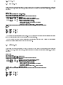
An X form will pop-up :
At this point you can modify (Edit parameters) or list the parameters (show parameters), or make other
actions by clicking on a button. Clicking on 'Edit parameters' or 'Show parameters' will pop-up another form
(see next page).
You can modify any elds. The modication is taken into account without doing a carriage return. It will
not accept parameters of an other type (integer, oat or string) than the type that has been dened for the
parameter when IDL rst read ao.par (see note 1 in the section ao.par). You may leave that parameter
window open and push buttons on the main simul window.
After having edited/modied the parameters (if necessary), you have to initialize before doing anything
else. Push the button initialize. The code will perform the functions described in the section 3.1, and
if ao.sim.monitor is set, it will display a contour of the subapertures with the electrode/actuator pattern
superimposed in the conguration window (if it has not exited in error because it didn't nd some le before
that).
Once initialized, you have to have a command matrix to start a loop. If the interaction and command matrices
have been restored (ao.zim.matrices set to a le name previously saved), you can skip the interaction matrix
acquisition and inversion steps. You may also invert the matrix again with dierent inversion parameters. This
will of course override the command matrix. If no matrices have been read, then you need to acquire one with
'Acquire interaction matrix', and invert it with 'Invert interaction matrix'. Again, be careful you have set the
deformable and tip-tilt mirror voltages to a suitable value. If ao.sim.monitor is set, the eigenvalues, the modes
corresponding to the zeroed eigenvalues, the interaction matrix and the command matrix will be displayed.
At this point, you may start a loop simulation. Once you click on 'Start loop', some initializations are done
and a message will appear on the 'loop' window, that tells you what operations can be entered while the loop
is running. Basically, you can update D=r0 (type d in the IDL root window), the loop gain (type g), the
extra-focal distance (CWFS only, type l), you can also reset the voltages on the mirrors (type r), toggle the
17
18
CHAPTER 4. RUNNING SIMUL
graphic display (type m) or stop the loop (type q). This also works when loop is started from the command
line.
Once done, you can change parameters and start again. It may not be clear for the user where to start from
when some parameters are changed : The following table gives a summary of the parameters, and where to
start from in the routine hierarchy (init, matrix acquisition, matrix inversion, loop, in this order) when the
parameter is modied.
Note concerning X window management into IDL : If the program exit in error while running simul with an
X form, you can always restore the control to the X form by typing
IDL> xmanager
This will give back the control to the event manager, and allow you to press new buttons.
4.2
Running Simul from the command line
can also be runned in a command line mode. This is especially useful to make batches, for instance to
test a serie of dierent parameter sets without continuous user interventions.
To start simul, type
IDL> simul
The code will read the parameter le ao.par and load the parameter default values into the ao structure. This
is the only purpose of the main routine simul.
For the ao structure to be accessible, you have to declare it at the main IDL level, by typing: IDL> common aostr,ao
simul
You may now change parameter values, e.g.
or start a subroutine, e.g.
IDL> ao.sim.monitor = 1
IDL> init
As described above, 4 subroutines are available : init, do_inter, mkmatcom and loop.
In this mode, 4 windows are created at the initalization level, to which the graphic displays will be directed
(if ao.sim.monitor = 1).
You may also include part of the commands, or all of the commands, in a batch. In IDL, starting a batch is
done by typing @ immediately followed by the name of the batch le. For instance,
IDL> @ao.batch
An example of a batch le is given below, and more examples are given in appendix A :
;
simul
common aostr,ao
ao.mir.def_file = 'bim_s64_p60_e80.fits'
ao.zim.matrices = 'mats_s64_p60_e80.fits'
ao.wfs.l = 0.30
ao.wfs.parfile = 'sensor.par.80'
ao.mir.parfile = 'mirror.par.80'
ao.atm.screen1 = 'screen14_f_800_200.fits'
init
;
;
ao.gs.starmag = 14.
ao.loop.gain
= 0.3
loop
;
4.2. RUNNING SIMUL FROM THE COMMAND LINE
Parameter name
19
Used in routines Parameter name
Used in routines
ao.zim.v_dm
do inter
ao.zim.v_tt
do inter
ao.zim.inversion
init
ao.zim.mta
init
ao.zim.mode_enable
mkmatcom
ao.zim.forcenev
mkmatcom
ao.zim.matrices
init
ao.mir.type
init
ao.mir.parfile
init
ao.mir.def_file
init
ao.mir.tt
init
ao.mir.v_limit
loop
ao.mir.nxact
init
ao.wfs.type
init
ao.wfs.geom
init
ao.wfs.parfile
init
ao.wfs.lambda
init
ao.wfs.nxsub
init
ao.wfs.pixsize
init
ao.wfs.subsize
init
ao.wfs.rnoise
do inter, loop
ao.wfs.blur
do inter, loop
ao.wfs.threshold
do inter, loop
ao.wfs.l
do inter, loop
ao.wfs.sinus
init
ao.wfs.fieldstop
loop
ao.wfs.mask
init
ao.gs.noise
loop
ao.gs.lgs (all)
init
ao.ttgswfs.(all)
init
ao.gs.extended
loop
ao.gs.gsmap
loop
ao.gs.gsmapscale
loop
ao.gs.starmag
loop, do inter
ao.gs.skymag
loop
ao.gs.zeropoint
loop, do inter
ao.tel.diam
init, do inter, loop ao.tel.cobs
init
ao.loop.type
loop
ao.loop.delay
loop
ao.loop.n_iter
loop
ao.loop.im_lambda
loop
ao.loop.aliasing
loop
ao.loop.gain
loop
ao.loop.start_skip
loop
ao.loop.it_time
loop
ao.atm.dr0
loop
ao.atm.directory
loop
ao.atm.screen1
loop
ao.atm.screen2
loop
ao.atm.screen3
loop
ao.atm.layer1_frac
loop
ao.atm.layer2_frac
loop
ao.atm.layer3_frac
loop
ao.atm.layer1_speed loop
ao.atm.layer2_speed loop
ao.atm.layer3_speed loop
ao.atm.layer1_alt
loop
ao.atm.layer2_alt
loop
ao.atm.layer3_alt
loop
ao.isop.enable
loop
ao.isop.diststar1
loop
ao.isop.diststar2
loop
ao.sim.size
init
ao.sim.pupd
init
ao.sim.monitor
ao.sim.calcmode
loop
ao.sim.calcmtf
loop
ao.sim.cb_output
loop
Table 4.1: Parameter names and routines that uses it. This is mostly to allow the user to determine if a new
initialization, or a new matrix, or nothing, is needed after updating parameters. 'init' stands for initialization,
'do inter' for 'acquire interaction matrix' and 'mkmatcom' for 'invert interaction matrix'.
20
CHAPTER 4. RUNNING SIMUL
ao.gs.starmag = 16.
ao.loop.gain = 0.15
loop
;
ao.gs.starmag = 18.
ao.loop.gain = 0.1
loop
;
In this batch, some environement parameters are modied (their default values specied in ao.par are overriden). Then, the routine init is called. In this example, the interaction and command matrices were computed
in a former run and stored in a le. This le (ao.zim.matrices) is here read by the init routine. The next step
is a serie of loop runs, with dierent magnitude values. At the complexion of each loop, results are appended
in a le called simul.res, as detailled in section 5.
4.3
Running time considerations
Note: this section was written in 1994. Things have changed some since then, but the order of the system we
want to simulate have also gone up, so it might still be lengthy to run simulations...
It is clear that you need a fast machine to run simul . You need also quite a bit of RAM space. 64 MB should
probably besuÆcient for reasonable application, but 128MB is better and is required for large system simulation
(128x128 arrays for instance). Simulating 36 subapertures CWFS on 64x64 arrays is fast (< 1s/iteration) on a
pentium equiped machine or a Ultra Sparc workstation. On the same machine, a SHWFS of 14x14 subapertures
on 128x128 arrays may take a couple of second per iteration.
This numerical simulation code is not intented to provide the user with a versatile tool. It is clear that the
running time, plus the necessity to have large statistical sample imply several minutes to several hours per
conguration. Hence a complete investigation of the parameter space, which contains quite a lot of parameters,
is diÆcult, if not impossible. The goal is more to precise/conrm results obtained with analytical code.
4.3. RUNNING TIME CONSIDERATIONS
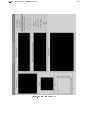
Figure 4.1: Main X form of the GUI
21
22
CHAPTER 4. RUNNING SIMUL
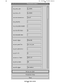
Figure 4.2: Parameter form
Chapter 5
The output les
These les are described in the introduction. As mentionned in there, simul.res contains a complete set of
information : Each time one of the routine is ran, it appends the results to simul.res, together with the
complete set of parameters. Parameters are loggued by writing the complete ao structure into the le. The
best is to run simul , and to have a look at simul.res le. It should be self explanatory.
23
24
CHAPTER 5. THE OUTPUT FILES
Appendix A
Batch Examples
This is a simple example of batch. It uses the batch command line language of IDL (not a procedure). To run
it, one should type IDL> @batch
The goal was here to investigate the performance at several WFS integration time.
; Start simul with parameter file ao.par.14x14
; Monitor is set to zero, so no graphic window is created.
simul,par='ao.par.14x14',mon=0
; define the common to be able to access the parameters at this level :
common aostr, ao
; Initialize
init
; Create a result summary file :
spawn,"echo 'results from batch_1' >! batch_1.res"
; Set the WFS integration time, run a loop and store the results :
ao.loop.it_time = 0.002
loop
spawn,"tail -2l simul.res >> batch_1.res"
; Same for a different WFS integration time, etc...
ao.loop.it_time
loop
spawn,"tail -2l
ao.loop.it_time
loop
spawn,"tail -2l
ao.loop.it_time
loop
spawn,"tail -2l
ao.loop.it_time
= 0.004
simul.res >> batch_1.res"
= 0.006
simul.res >> batch_1.res"
= 0.008
simul.res >> batch_1.res"
= 0.010
25
26
loop
spawn,"tail -2l
ao.loop.it_time
loop
spawn,"tail -2l
ao.loop.it_time
loop
spawn,"tail -2l
ao.loop.it_time
loop
spawn,"tail -2l
APPENDIX A. BATCH EXAMPLES
simul.res >> batch_1.res"
= 0.020
simul.res >> batch_1.res"
= 0.040
simul.res >> batch_1.res"
= 0.080
simul.res >> batch_1.res"
27
This is a quite elaborated example already : The goal was here to investigate the performance of several
subaperture congurations for a 36 or so curvature system.
pro optim36
; define the common to be able to access the parameters :
common aostr, ao
; Create a file named ``optim36.res'' to summarize the results :
com = "echo resultats optim >! optim36.res"
res = execute('spawn,com')
; Start simul (this reads out the par file and put the variable into
; the common area :
simul,par='ao.par.optim.l30.s0'
; define the configurations I want to evaluate :
configs = [[4,6,10,16], $
[1,6,12,18], $
[1,6,12,16], $
[2,6,10,18], $
[3,6,10,18], $
[3,6,12,16], $
[2,6,12,16]]
nconfigs= (size(configs))(2)
frint = [1.,0.9,0.8,1.1]
frext = [1.,1.1,1.2,0.9]
; loop on the configurations :
for i=0,nconfigs-1 do begin
; load the current configuration :
config = configs(*,i)
; Some formating of the summary file :
openw,1,'optim36.res',/append
printf,1,'++++++++++++++++++'
printf,1,config
close,1
; loop on ring radius within a given configuration :
for j=0,3 do begin
r = cwfs_design(config,0.1365)
r(0) = r(0)*frint(j)
r(n_elements(r)-1) = r(n_elements(r)-1)*frext(j)
28
APPENDIX A. BATCH EXAMPLES
; write the mirror and sensor par file for this configuration
write_parfiles,config,r
; Initialize in 'modal' to get the mode to actuator matrix and mode
; expression. This is to get the propagation of the noise.
ao.zim.inversion = 'modal'
ao.sim.calcmode = 1
ao.zim.mta
= ''
init
do_inter
mkmatcom
; make the command matrix to be used in 'zonal'
ao.zim.inversion = 'zonal'
ao.sim.calcmode = 0
mkmatcom
; run the loop
loop
; grab the results from the output files and put
; them in the results summary file.
openw,1,'optim36.res',/append & printf,1,r & close,1
com = "cat modes_noise.dat >> optim36.res"
res = execute('spawn,com')
com = "tail -2l simul.res >> optim36.res"
res = execute('spawn,com')
endfor
endfor
com = "mv optim36.res optim36.res.l30.s0"
res = execute('spawn,com')
end
;-------------------------pro write_parfiles,config,r
; this is a procedure that writes par files (sensor and mirror) for
; a given config according to the format recognized by simul.pro.
; Just to avoid to pre-type them all.
n = n_elements(config)
rint = shift(r,1)
rint(0.)= 0.
rext = r
rext(n-1) = 1.5
openw,1,'sensor.par'
printf,1,'.start.'
printf,1,'R'
29
printf,1,n_elements(config),format='(i1)'
for i=0,n_elements(config)-1 do $
printf,1,rint(i),rext(i),config(i),0.,1,format='(f4.2,3x,f4.2,3x,i3,3x,f3.1,3x,i1)'
close,1
rint(n-1) = 1.0
rext(n-1) = 1.6
openw,1,'mirror.par'
printf,1,'.start.'
printf,1,n_elements(config),format='(i1)'
printf,1,'0 0'
for i=0,n_elements(config)-1 do $
printf,1,rint(i),rext(i),config(i),0.,1,format='(f4.2,3x,f4.2,3x,i3,3x,f3.1,3x,i1)'
printf,1,'1.8'
close,1
end