Download Project Manual

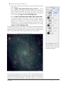
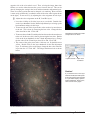
M33 Tutorial
Making Color Images
Travis A. Rector
University of Alaska Anchorage and NOAO
Department of Physics and Astronomy
3211 Providence Dr., Anchorage, AK USA
email: [email protected]
Introduction
A Note from the Author
The purpose of this tutorial is to demonstrate how color images of astronomical
objects can be generated from the original FITS data files. The techniques described
herein are used to create many of the astronomical images you see from professional observatories such as the Hubble Space Telescope, Kitt Peak, Gemini and
Spitzer. In this tutorial we will make an image of M33, the Triangulum Galaxy.
M33 is a spectacular face-on spiral galaxy that is relatively nearby.
It is assumed that you are familiar with the prerequisites listed below. If you
have problems with the tutorial itself please feel free to contact the author at the
email address above.
Prerequisites
To participate in this tutorial, you will need a basic understanding of the following concepts and software:
The WIYN 0.9-meter Telescope
Nomenclature:
FITS stands for Flexible Image
Transport System. It is the standard format for storing astronomical data.
• FITS datafiles
• Adobe Photoshop or Photoshop Elements
• The layering metaphor
Description of the Data
The datasets of M33 used in this tutorial were obtained with the WIYN 0.9-meter
telescope on Kitt Peak, which is located about 40 miles west of Tucson, Arizona.
The FITS files are 2048 x 2048 pixels, and about 16 Mb in size each. Datasets in
the broadband UBVRI and narrowband Ha filters are available. For this tutorial
we will use only the B, V and Ha datasets. But you are encouraged to play with
the other datasets afterwards.
Decoding file names
The FITS filenames consist of the
name of the object, an underscore,
and then the filter name. For
example, the m33_ha FITS file
is M33 in the H-alpha filter.
These datasets are provided to be used strictly for educational purposes. They
may not be redistributed without permission. If you wish to use these files for
other purposes please contact the author.
About the Software
This tutorial requires Adobe® Photoshop® (version 7.0 and later) or Adobe Photoshop Elements (version 2.0 and later). Both run on the Macintosh (OS 9 and
OS X) and PC (Microsoft Windows) platforms. In this tutorial Photoshop CS3
will be used, but it is very similar for Photoshop Elements. Differences between
the two programs are occasionally noted in the sidebar.
Rev 4/1/08
Image Tutorial 1
This tutorial also requires the ESA/ESO/NASA FITS Liberator. It is a plug-in
for Photoshop and Photoshop Elements that enables these programs to import
FITS data files. The current version is v2.1. The FITS Liberator is free and can
be downloaded at http://www.spacetelescope.org/projects/fits_liberator/ A more
in-depth instruction manual on all of the capabilities of the FITS Liberator is
also available at that URL. Be sure that this plug-in is properly installed before
starting the tutorial.
Description of the Image-Making Process
When people see astronomical images they often ask: “Is that what it really looks
like?” The answer is always no. This is because our telescopes are looking at
objects that are usually too faint, and often too small, for our eyes to see. Furthermore, our telescopes can also “see” kinds of light that our eyes cannot, such
as radio waves, infrared, ultraviolet and X-rays. In a sense, telescopes give us
“super human” vision. Indeed, that’s why we build them!
It is important to note that telescopes work very differently than a traditional
camera. The instruments on our telescopes are designed to detect and measure
light. We must then take the data that comes from the telescope and translate it
into an image that our eyes can see, and our minds can understand.
Note!
Many of the steps described in this
process are subjective. They are
based upon the color calibration
of the author’s computer display,
and his personal aesthetics. If
your final image does not look
pleasing, it is either because you
did not follow a step correctly, your
computer’s monitor is not properly
calibrated (many monitors are
too dark), or you do not share
the author’s excellent aesthetic
palette.
Astronomical images are made in a very different way than they were even just
twenty years ago. Instead of film or photographic plates we use electronic instruments, such as CCD (“charge-coupled device”) cameras. In addition to their
better sensitivity, these electronic devices also produce data that can be analyzed
on a computer. Finally, thanks to the tremendous leaps in computing power and
in image-processing software, it is now possible to produce high-quality color
images of astronomical objects in a purely digital form.
One particular advantage of image-processing software, such as Photoshop, is
that they use a “layering metaphor” for assembling images. In this system, individual images, which are stored as separate layers, may be combined to form a
single image. Before this, color images could only be assembled from only three
grayscale images. And each image could only be assigned to the “channel” colors
of red, green and blue. With the layering metaphor, it is possible to combine any
number of images. And each image may be assigned any color you like. The
layering technique has been used to produce astronomical images with as many
as eight different images. Each image is produced from a different dataset, each
of which shows different details in the astronomical object. Such images are
therefore richer in color and detail. This tutorial explains how its done.
The steps followed to produce a color image can be summarized as:
• Import each dataset to be used into Photoshop using the FITS Liberator.
The image from each dataset will be stored as a separate layer.
• Rescale each layer to maximize the contrast and detail in the interesting
parts of the image.
• Assign a different color to each layer.
• Fine tune the color balance of the image.
• Align the image layers and remove any cosmetic defects.
Each step is described in detail below. Note: In this document an “ì” icon
appears when a computer command is described.
2 Image Tutorial
Rev 4/1/08
Importing Datasets with FITS Liberator
Adobe Photoshop by itself cannot open FITS files. This is because FITS is a
data file format, not an image format. The FITS Liberator is a plug-in that converts the pixels in a FITS file into pixels for an 8 or 16-bit grayscale image. In
a FITS file the pixels may have any value they want, including negative values.
In an 8-bit grayscale image, the pixels may only be one of 256 possible values.1
Thus, a mathematical function, often called a “transfer” or “stretch” function,
must be used to convert the data pixel values in the FITS files into grayscale
image pixel values.
Nomenclature:
Clipping refers to the pixel values
that are outside the range between
the black and white points.
Pixels below the black point
(shown in blue) will be set to a pure
black when imported into Photoshop. And pixels above the white
point (shown in green) will be set
to a pure white. These pixels are
said to be ‘clipped’ because you
will not be able to see any detail
in these clipped regions.
In brief, make sure the black and
white points are set so that there
are very few blue or green pixels
in the image.
ì Launch Adobe Photoshop.
ì Import the B-filter file of M33 with FITS Liberator:
• Choose File/Open... and select ‘m33_b.fits’ data file. A window should
appear that looks similar to the one shown above. If you are unable to
select the ‘m33_b.fits’ file, or if the above window does not appear, you
may not have the FITS Liberator properly installed.
• Change the stretch function to ‘Log(x)’.
• On the right side of the image make sure that the ‘Undefined (red),’
‘White clipping (green),’ and ‘Black clipping (blue)’ check boxes are
all selected.
• You should now see blue and green pixels on the image. Move the black
level slider (under the histogram) so that the Black Level (shown in the
lower-left corner) is 2.35. Most of the blue pixels in the image should
now be gone.
• Move the white level slider (also under the histogram) all the way to the
right so that the White Level (shown at the bottom) is 4.77. Most of the
green pixels in the image should now be gone.
Scaled Peak Level
The scaled peak level adjusts the
contrast in the image. A small
scaled peak level means there
is high contrast (better detail) in
the bright parts of the image, but
poorer contrast (less detail) in the
faint parts of the image. A large
scaled peak level does just the
opposite. Thus, the scaled peak
level should be adjusted to best
show the detail in the bright and
faint parts of the image.
• Click the ‘Auto Scaling’ button. The image above should now appear
nearly black. To increase the contrast in the faint parts of the image,
change the ‘Scaled Peak level’ to 1000 and hit return (do not click on
1
This is because 28 = 256. In a 16-bit image, 65,536 (216) values are available.
Rev 4/1/08
Image Tutorial 3
the Auto Scaling button again because it will reset the scaled peak level
back to 10). The image should be brighter, the Black Level should be
0.00 and the White Level should be 3.00. The window should look like
what is shown below.
• If you are using Photoshop 7.0 or Photoshop Elements, change the Channels (bottom center) to 8 bit. Otherwise leave it as 16 bit.
• Click ‘OK’ and the image will be imported into Photoshop.
Preparing the Main Image File
You should now see a grayscale image of M33. This is only one of the three
images we will import into Photoshop. Before we import the others we must
prepare this image to become the main image file:
ì Prepare the main image file:
• If it is not visible already, choose Window/Layers to make the layers
window visible. A single layer should be present, titled ‘background.’
The layers window in Photoshop
after the background layer has
been renamed.
• In the layers window, double click on the background layer. A dialog
box titled ‘New Layer’ will appear. Rename the layer to ‘B log(1000)’.
This will be useful later for keeping track of which layer is which.
• Currently Photoshop considers this image to be grayscale, and therefore
disables the functions related to color. Choose Image/Mode/RGB
Color to convert the image into a color image. Note: This won’t change
the appearance of the image. It simply prepares the image so that it can
be make into a color image later on.
• Now it is time to save the tutorial image as a separate file. Choose File/
Save As... to save the image as a Photoshop document. In the dialog
box, choose the directory into which you want to save the image. Name
the file ‘m33_demo.psd.’ Make sure the format is set to ‘Photoshop’ and
the ‘Layers’ box is checked. Don’t worry about the other check boxes.
Rev 4/1/08
Note!
You may also see an extra dialog
box that asks you if you wish to
maximize the compatibility of the
file image. If you see this, go ahead
and select yes.
Image Tutorial 4
The image should look as shown above. We will fine tune the intensity scaling
later.
Importing the Other Datasets
Now it is time to import the other datasets and copy them into the main image
file. We will start with the V-band dataset:
ì Import the V-filter file of M33 with FITS Liberator:
• Choose File/Open... and select ‘m33_v.fits’ data file. The FITS
Liberator window should appear. Make sure that the ‘Undefined (red),’
‘White clipping (green),’ and ‘Black clipping (blue)’ check boxes are all
selected.
• Change the stretch function to ‘Log(x)’.
• Move the black level slider so that the Black Level is 2.54. Most of the
blue pixels in the image should now be gone.
• Move the white level slider so that the White Level is 4.79. Most of the
green pixels in the image should now be gone.
• Click the ‘Auto Scaling’ button. The image above should now appear
nearly black. To get the same contrast as the B layer, change the ‘Scaled
Peak level’ to 1000 and hit return (remember, do not click the Auto Scaling button again).
• If you are using Photoshop 7.0 or Photoshop Elements, change the Channels (bottom center) to 8 bit. Otherwise leave it as 16 bit.
• Click ‘OK’ and the image will be imported into Photoshop.
• In the layers window, rename the layer to ‘V log(1000)’.
Rev 4/1/08
Image Tutorial 5
The V-band grayscale image now needs to be copied into the main image file:
ì Choose Layer/Duplicate Layer... and a dialog box will appear.
Change the destination to ‘m33_demo.psd’ and click ‘OK’. Now the
V-band image is copied into the main image file so we can get rid of this
copy. Choose File/Close and Photoshop will ask you if you wish to
save the image. Click on ‘Don’t Save.’
The B-band and V-band grayscale images are now loaded into the main image
file, each as a separate layer. Finally, import the Ha image and duplicate it into
the main image file:
ì Import the Ha-filter file of M33 with FITS Liberator:
• Choose File/Open... and select ‘m33_ha.fits’ data file. The FITS
Liberator window should appear. Make sure that the ‘Undefined (red),’
‘White clipping (green),’ and ‘Black clipping (blue)’ check boxes are all
selected.
• Change the stretch function to ‘Log(x)’.
• Move the black level slider so that the Black Level is 1.47. Most of the
blue pixels in the image should now be gone.
• Move the white level slider so that the White Level is 3.70. Most of the
green pixels in the image should now be gone.
• Click the ‘Auto Scaling’ button. Change the ‘Scaled Peak level’ to 1000
and hit return (do not click the Auto Scaling button again).
• If you are using Photoshop 7.0 or Photoshop Elements, change the Channels (bottom center) to 8 bit. Otherwise leave it as 16 bit.
• Click ‘OK’ and the image will be imported into Photoshop.
• In the layers window, rename the layer to ‘ha log(1000)’.
• Choose Layer/Duplicate Layer... and a dialog box will appear.
Change the destination to ‘m33_demo.psd’ and click ‘OK’. Now that
the Ha-band image is copied into the main image file we can get rid of
it. Choose File/Close and Photoshop will ask you if you wish to save
the image. Click on ‘Don’t Save.’
All three grayscale image should now be in the main image file. The layers window
should look as shown on the right. However, you will only see the image in the
top layer. This is because the blending mode for each layer is set by default to
‘Normal.’ (The blending mode menu is the one at the top of the layers window.)
For the light from the images in each layer to combine, the blending mode for
each layer must be set to ‘Screen’:
ì Select the ‘ha log(1000)’ layer by clicking on it. Change the blending
mode from ‘Normal’ to ‘Screen.’ Change the modes for the other layers
as well by selecting each layer and changing its blending mode. The
opacity of each layer should be kept at 100%. (Note: Technically you
don’t need to change the blending mode of the bottom layer, but you
might as well do it anyway in case you change the order of the layers.)
The layers window in Photoshop
after the V-band and Ha images
has been duplicated into the main
image file.
The image will be much brighter now because the screen mode for each layer
“adds” the intensity of the that layer to the overall image. You can see the effect
of each layer on the overall image by turning on and off the visibility of each
Rev 4/1/08
Image Tutorial 6
layer. This is done by clicking on the eyeball on the left side of each layer (in the
layer window). When all of the layers are visible (i.e., when there is an eyeball
visible next to each layer), the image should look as shown on the next page:
Nomenclature:
Contrast is a measure of how well
differences in brightness can be
seen. In a high-contrast image,
even small differences in brightness can be seen.
Dynamic range is the ratio of the
intensity in the brightest region to
the darkest region.
If you have not done so recently, this is an excellent time to save the image.
Contrast and dynamic range are
at odds with each other. Overall,
an image with high dynamic range
will have a low contrast, and vice
versa. The ‘levels’ and ‘curves’
tools are used to maximize the
contrast in the interesting parts
of the image, while maintaining a
high dynamic range for the overall
image.
Rescaling and Colorizing Each Layer
Now that a grayscale image for each filter is loaded as a layer into the main image
file, it is time to fine tune the intensity scaling for each layer so that we can best
see the details in the faint and bright parts of each layer. This is best done by
working with only one layer visible at a time:
ì Rescale the intensity of the B-band layer:
• Turn off the visibility of the V and Ha layers. There should only be an
eyeball next to the B layer.
• Select the B layer by clicking it. It should be the one highlighted.
• Choose Layer/New Adjustment Layer/Levels... A ‘New
Layer; dialog box will appear. Click ‘OK’ and a new window will appear.
A histogram will be shown in the ‘Input Levels’ area of the window. Like
in the FITS Liberator, you can use the sliders underneath the histogram
to move the black and white points. You’ll also see a gray slider that
adjusts the ‘gamma’ correction.
• Move the black slider a little to the right. As you move the slider you’ll
Rev 4/1/08
Image Tutorial 7
notice the image gets darker. Move it until the number below the black
point is 8. This is done so that the image will be almost completely black
in the darkest portions of the image, e.g., in the lower-left corner.
• Move the gray slider a little to the left. As you move the slider you’ll
notice the image gets a little brighter. Specifically, the contrast in the
faint regions is increasing, and the contrast in the dark regions is decreasing. The number below the gray point (known as the gamma correction)
should be about 1.32. This is done to improve the contrast in the center
of the galaxy.
• Do not move the white slider. The white point should remain at 255. And
don’t change the Output Levels. The window should look as shown:
Note!
In Photoshop Elements the imput
levels will be above the histogram
in the dialog box to the left.
• Click ‘OK’ and a new layer will appear above the B-band layer.
The new layer is called an ‘adjustment layer.’ It does not consist of an image;
rather, it adjusts the appearance of the layers below it. You can see the effect of
the adjustment layer by toggling the visibility of the layer (i.e., clicking on and
off the eyeball for the adjustment layer.) The effect of the adjustment layer is
that it improves the contrast in the center of the galaxy while keeping the outer
edges of the galaxy from getting too bright.
An adjustment layer will affect all of the layers below it. The ‘Levels 1’ adjustment layer must therefore be grouped to the B-band layer so it only adjusts it.
(Note: For the B-band image layer this is not a problem because there are no
other layers below it, but it will be an issue for the other image layers.)
ì Select the ‘Levels 1’ adjustment layer by clicking on it. Choose Layer/
Create Clipping Mask. The adjustment layer will indent; and an
arrow will point down to the B-band image layer.
Finally, we will assign a color to the layer. This is done with the ‘Hue/Saturation’ adjustment layer:
Note!
In Photoshop Elements the menu
option is called Layer/Create
Clipping Mask. You can also
select this option in the levels
dialog box.
ì Assign a blue color to the B-band layer:
• Select the ‘Levels’ layer above the B-band layer by clicking it. It should
be the one highlighted.
• Choose Layer/New Adjustment Layer/Hue/Saturation...
A ‘New Layer; dialog box will appear. Click ‘OK’ and a new window
will appear. A window will appear that has three sliders for hue, saturation and lightness.
Rev 4/1/08
Image Tutorial 8
• Before moving any of the sliders click on the ‘Colorize’ checkbox in the
lower-right corner of the window. The image will go red.
• Once the colorize checkbox is selected, the hue slider will determine
what color they layer will be. The numbers correspond to an angle on
the color wheel between 0° and 360° (see the figure to the right). Since
this is the blue filter set the hue to 240. The image will turn blue.
• Set the saturation to 100 and the lightness to -50. This will make the
image a dark, deep blue. The window should look as shown below:
The angles around the color wheel
correspond to hue values.
• Click ‘OK’. A new adjustment layer titled ‘Hue/Saturation 1’ will appear
above the ‘Levels 1’ layer.
• Select the ‘Hue/Saturation 1’ adjustment layer by clicking on it. Choose
Layer/Create Clipping Mask. The adjustment layer will indent;
and an arrow will point down to the ‘Levels 1’ image layer.
Since the ‘Levels 1’ and ‘Hue/Saturation 1’ adjustment layers are grouped to
B-band layer they will only adjust that layer. The layers window should look
as shown to the right.
Now its time to rescale and colorize the V-band and Ha layers by following the
same steps as described above for the B-band layer:
ì Rescale and colorize the V-band layer:
• Turn off the visibility of the B-band layer. Select the V-band layer and
turn on its visibility.
• Choose Layer/New Adjustment Layer/Levels... A ‘New
Layer; dialog box will appear. Click ‘OK’ and the levels window will
appear. To darken the background and increase the contrast in the faint
parts of the galaxy, set the black point to 35 and the gray point to 1.23.
Do not move the white point. Click ‘OK’ and then group the levels
adjustment layer by choosing Layer/Create Clipping Mask.
• Choose Layer/New Adjustment Layer/Hue/Saturation...
A ‘New Layer; dialog box will appear. Click ‘OK’ and the hue/saturation window will appear. Click on the ‘Colorize’ checkbox. Since the
V-band filter is green, set the hue to 120. Set the saturation to 100 and
the lightness to -50. This will make the image a dark, deep green. Click
‘OK’ and then group the hue/saturation adjustment layer by choosing
Layer/Create Clipping Mask.
Rev 4/1/08
The layers window in Photoshop
after the B-band layer has been
rescaled and colorized. The Ha
and V layers have not yet been
rescaled and colorized.
Image Tutorial 9
ì Rescale and colorize the Ha layer:
• Turn off the visibility of the V-band layer. Select the Ha layer and turn
on its visibility.
• Choose Layer/New Adjustment Layer/Levels... A ‘New
Layer; dialog box will appear. Click ‘OK’ and the levels window will
appear. Set the black point to 61 and the gray point to 1.05. Do not
move the white point. Click ‘OK’ and then group the levels adjustment
layer by choosing Layer/Create Clipping Mask.
• Choose Layer/New Adjustment Layer/Hue/Saturation...
A ‘New Layer; dialog box will appear. Click ‘OK’ and the hue/saturation window will appear. Click on the ‘Colorize’ checkbox. Since the
Ha filter is red, set the hue to 0. As before, set the saturation to 100 and
the lightness to -50. This will make the image a dark, deep red. Click
‘OK’ and then group the hue/saturation adjustment layer by choosing
Layer/Create Clipping Mask.
Each image has now been rescaled and colorized. Make sure that each adjustment
layer is grouped to the image layer below it. To see how the overall image looks
turn on the visibility of the B-band and V-band layers. The layers window should
look as shown on the right; and the image should look as shown below:
The layers window in Photoshop
after all three layers have been
rescaled and colorized.
Its not bad, but the galaxy has too much cyan. This is because the B-band and
V-band filters primarily show the stars in the galaxy, whereas the Ha filter primarily shows the warm hydrogen gas in the galaxy (where stars are forming).
Thus the stars will look cyan, which is a mix of blue and green. Cyan is on the
Rev 4/1/08
Image Tutorial 10
opposite side of the color wheel as red. Thus, to bring the image better into
balance, we need to either decrease the cyan or increase the red. This can be
done by changing the setting in the levels and hue/saturation adjustment layers.
There are so many options that can be changed, it is confusing. How to do this
is more easily understood if you think in terms of the color wheel (again shown
on the right). To start we’ll try by adjusting the color assigments to each layer:
ì Adjust the color assignments to the B, V and Ha layers:
• Leave the visibility of all of the layers on as you do this. Double click
on the layer thumbnail for the B-band adjustment layer to bring up the
hue/saturation settings for this layer.
• To increase the red in this layer the hue value needs to be moved more
to the red. This is done by increasing the hue value. Change the hue
value from 240 to 260. Click ‘OK’.
• To increase the red in the V-band layer the hue also needs to be moved more
to the red. In this case, this is done by decreasing the hue value. Double
click on the layer thumbnail for the V-band adjustment layer. Change
the hue value of the V-band layer from 120 to 100. Click ‘OK’.
The angles around the color wheel
correspond to hue values.
• The center of the galaxy now looks a little too red. It should be more
yellow. Double click on the layer thumbnail for the Ha adjustment
layer. To add more yellow to the image, change the hue value of the Ha
layer from 0 to 15. Click ‘OK’. The image should now look as shown
below.
Layer thumbnail
Layer mask
thumbnail
Caution!
If you double-click on the layer
mask thumbnail (the white square
to the right of the layer thumbnail)
a ‘Layer Mask Display Options’
window will appear. If this occurs,
click ‘Cancel’ and try again.
Rev 4/1/08
Image Tutorial 11
The colors are now more in balance. The image may also be improved by
adjusting the black and gray points (gamma correction) of the level adjustment
layers. Because this image uses only three datasets, the image can be vastly
improved by using the additional M33 datasets. These should be imported,
rescaled and colorized in the same manner. Finally, there are many additional
tools that are available in Photoshop (e.g., the ‘curves’ tool) that enable the
layers to be manipulated more precisely. For simplicity these methods and
tools are not discussed here.
As always, this is an excellent time to save the image.
Fine Tuning the Image
The image is mostly done, but there are still several steps necessary to complete
the image. One issue that has not yet been addressed is the alignment of the
image layers. Because these images were taken with the same telescope and
camera, and on the same night one after another, the images are already very
closely aligned. However, if you zoom in on the image (say, to 500%, as shown
on the right) you will notice that the stars are not perfectly aligned. To align
the images use the ‘move tool’ to shift each image layer so that they are aligned
with one another. (Note: Shifting the adjustment layers will have no effect):
Zooming into the image to 500%
shows that the stars are not
aligned. Use the ‘move tool’ in
Photoshop to align the image
layers.
ì Select the Ha layer by clicking on it. Choose the ‘move tool’ and use
the arrow keys to shift the layer until it is well aligned with the B-band
layer. Now select the V-band layer and shift it as well so that it is aligned
with the other two.
Zooming will also reveal that there are numerous dots and small streaks in the
image. These are caused by cosmic rays that hit the CCD detector during each
exposure. They are therefore in different locations in each filter image and
therefore have a color that matches that filter; e.g., cosmic rays in the V-band
image look green. In the case of this image, nearly all of the cosmic rays are in
the V-band image.
These ‘cosmic ray’ specs and scratches can be fixed in a variety of ways in
Photoshop. A simple option is to use one of the noise filters; e.g., the ‘dust and
scratches’ filter. These can remove the cosmic rays, but they also blur the image.
A more effective but time-consuming method is to use the cloning stamp and
healing brush tools to remove the cosmic rays one by one. The user’s manual
for Photoshop explains how these tools are used.
Rev 4/1/08
Image Tutorial 12