Download for GIMP - Australian Gemini Office

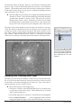
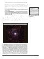
NGC 6751 Tutorial
Making Color Images
Christopher A. Onken
Travis A. Rector
The Australian National University
University of Alaska Anchorage
Mount Stromlo Observatory
Department of Physics and Astronomy
Cotter Rd., Weston Creek, ACT Australia
3211 Providence Dr., Anchorage, AK USA
email: [email protected]
email: [email protected]
Introduction
The Gemini South Telescope
A Note from the Authors
The purpose of this tutorial is to demonstrate how color images of astronomical objects can be generated from the original FITS data files. The techniques
described herein are used to create many of the astronomical images you see
from professional observatories such as the Hubble Space Telescope, Kitt Peak
National Observatory, and Gemini Observatory. In this tutorial we will make an
image of NGC 6751, a planetary nebula in the constellation of Aquila, the eagle.
It is assumed that you are familiar with the prerequisites listed below. If you have
problems with the tutorial itself please feel free to contact the authors.
Prerequisites
To participate in this tutorial, you will need a basic understanding of the following concepts and software:
• FITS datafiles
• GIMP - The GNU Image Manipulation Program
• The layering metaphor
Description of the Data
The datasets of NGC 6751 used in this tutorial were obtained with the Gemini
South 8.1-meter telescope, which is located at the summit of Cerro Pachón, Chile.
The FITS files are 3108 x 2304 pixels, and about 28.7 Mb in size each. Datasets
in the narrowband Ha, [OIII] and [SII] filters are available for this object. These
data were obtained for the winning picture of the 2009 Gemini School Astronomy
Contest in Australia.
About the Software
This tutorial requires GIMP, which is available for the Macintosh, Windows,
and Unix/Linux platforms. The software is free and can be downloaded from
http://www.gimp.org/ In this tutorial, GIMP v2.6 will be used.
This tutorial also requires the ESA/ESO/NASA FITS Liberator. It is a program
that coverts FITS data files into TIFF image files. The current version is v3.0.
The FITS Liberator is free and can be downloaded at http://www.spacetelescope.
org/projects/fits_liberator/ An instruction manual is also available at that URL.
Rev 25 Jan 2012
Nomenclature:
FITS stands for Flexible Image
Transport System. It is the standard format for storing astronomical data.
Nomenclature:
“Ha“ is pronounced “hydrogen
alpha” or “H alpha”. It is a specific
color of red light produced by
warm hydrogen atoms. “[OIII]”
is pronounced “oxygen three” or
‘O three” and is a specific color
of green light produced by hot
oxygen atoms. And “[SII]” is pronounced “sulfur two” or “S two”.
It is a specific color of red light
produced by hot sulfur atoms.
These are kinds of light commonly
produced by planetary nebulae.
Decoding file names
The FITS filenames consist of the
name of the object, an underscore,
and then the filter name. For
example, the ngc6751_ha FITS
file is the data for NGC 6751 in
the H-alpha filter.
Image Tutorial
1
Description of the Image-Making Process
When people see astronomical images they often ask: “Is that what it really
looks like?” The answer is always no. This is because our telescopes are looking at objects that are usually too faint, and often too small, for our eyes to see.
Furthermore, telescopes can also “see” kinds of light that our eyes cannot, such
as radio waves, infrared, ultraviolet and X-rays. In a sense, telescopes give us
“super human” vision. Indeed, that’s why we build them!
It is important to note that telescopes work differently than a traditional camera.
The instruments on our telescopes are designed to detect and measure light. We
must then take the data that comes from the telescope and translate it into an
image that our eyes can see, and our minds can understand.
Astronomical images are made in a very different way than they were even just
twenty years ago. Instead of film or photographic plates we use electronic instruments, such as CCD (“charge-coupled device”) cameras. In addition to their
better sensitivity, these electronic devices also produce data that can be analyzed
on a computer. Finally, thanks to the tremendous leaps in computing power and
in image-processing software, it is now possible to produce high-quality color
images of astronomical objects in a purely digital form.
Note!
Many of the steps described in this
process are subjective. They are
based upon the color calibration
of the authors’ computer displays,
and their personal aesthetics. If
your final image does not look
pleasing, it is either because you
did not follow a step correctly, your
computer’s monitor is not properly
calibrated (many monitors are
too dark), or you do not share
the authors’ excellent aesthetic
palettes.
One particular advantage of image-processing software, such as GIMP, is that
they use a “layering metaphor” for assembling images. In this system, individual
grayscale images, which are stored as separate layers, may be combined to form
a single image. Before this, color images could only be assembled from only
three grayscale images. And each grayscale image could only be assigned to the
“channel” colors of red, green and blue. With the layering metaphor, it is possible
to combine any number of images. And each image may be assigned any color
you like. The layering technique has been used to produce astronomical images
with as many as eight different images. Each image is produced from a different
dataset, each of which shows different details in the astronomical object. Such
images are therefore richer in color and detail. This tutorial explains how its done.
The steps followed to produce a color image can be summarized as:
• Convert each FITS dataset into a grayscale TIFF image using the FITS
Liberator.
• Open each TIFF image with GIMP. The image generated from each
dataset will be stored as a separate layer in a single GIMP image.
• Rescale each layer to maximize the contrast and detail in the interesting
parts of the image.
• Assign a different color to each layer.
• Fine tune the color balance of the image.
• Remove any cosmetic defects.
Each step is described in detail below. Note: In this document an “” icon
appears when a computer command is described.
2 Image Tutorial
Rev 25 Jan 2012
Converting Datasets with FITS Liberator
Before using GIMP to play with the images, we will use another piece of software
to convert the raw images to a format other than FITS. This is because FITS is
a data file format, not an image format. The FITS Liberator is a program that
converts the pixels in a FITS file into pixels for an 8-bit or 16-bit grayscale image.
In a FITS file the pixels may have any value they want, including negative values.
In an 8-bit grayscale image, the pixels may only be one of 256 possible values.1
Thus, a mathematical function, often called a “transfer” or “stretch” function,
must be used to convert the data pixel values in the FITS files into grayscale
image pixel values.
Nomenclature:
Clipping refers to the pixel values
that are outside the range between
the black and white points.
Pixels below the black point
(shown in blue) will be set to a pure
black when imported into GIMP.
And pixels above the white point
(shown in green) will be set to a
pure white. These pixels are said
to be ‘clipped’ because you will
not be able to see any detail in
these clipped regions.
In brief, make sure the black and
white points are set so that there
are very few blue or green pixels
in the image.
Import the Ha-filter file of NGC 6751 with FITS Liberator:
• Launch FITS Liberator. Choose File/Open... and select ‘ngc6751_
ha.fits’ data file. The window should look similar to shown above. If
you are unable to select the ‘ngc6751_ha.fits’ file, or if the above window
does not appear, you may not have the FITS Liberator properly installed.
Note that there are gray edges on the left and right sides of the images.
These aren’t important to us and we’ll trim them off in GIMP later.
• If it is not set to it already, change the stretch function to ‘Log(x)’.
• On the right side of the image make sure that the ‘Undefined (red),’
‘White clipping (green),’ and ‘Black clipping (blue)’ check boxes are
all selected. Make sure the ‘flip image’ and ‘freeze settings’ options are
not selected.
• You should now see blue and green pixels on the image. Move the black
level slider (under the histogram) to the left until most of the blue pixels
in the image are gone. It is ok if you have a small sprinkling of blue
pixels through the image, or blue pixels along the edge of the image.
Scaled Peak Level
The scaled peak level adjusts the
contrast in the image. A small
scaled peak level means there
is high contrast (better detail) in
the bright parts of the image, but
poorer contrast (less detail) in the
faint parts of the image. A large
scaled peak level does just the
opposite. Thus, the scaled peak
level should be adjusted to best
show the detail in the bright and
faint parts of the image.
• Move the white level slider (also under the histogram) to the right until
most of the green pixels in the image should now be gone. It is ok if
you have a small sprinkling of green pixels through the image, or green
1
This is because 28 = 256. In a 16-bit image, 65,536 (216) values are available.
Rev 25 Jan 2012
Image Tutorial
3
pixels along the edge of the image
• Click the ‘Auto Scaling’ button. The image above should now appear
nearly black. To increase the contrast in the faint parts of the image,
change the ‘Scaled Peak level’ from 10 to 10000 and hit return (do not
click on the Auto Scaling button again because it will reset the scaled
peak level back to 10). The image should be brighter, the Black Level
should be 0.00 and the White Level should be 4.00. The window should
look close to what is shown below.
• Change the Channels (bottom center) to 8 bit.
• Click the ‘Save As...’ button and save the file as ‘ngc6751_ha.tiff’.
• Repeat the above steps for the [OIII] and [SII] images. Again, when
moving the black point and white point sliders choose settings so that
there are few blue and green pixels in the image.
Loading the Images into GIMP
The layers window in GIMP after
the background layer has been
renamed.
You should now have three TIFF files, one for each dataset. If you want your
final image to look exactly as shown in the tutorial, you may use the TIFF files
inclued with the tutorial. Note: when opening the pre-packaged TIFF files, you
will see a warning that GIMP has converted the image to 8 bits per channel,
since GIMP cannot process 16-bit files. These were generated using the above
instructions. We will now open the three TIFF images with GIMP. Before we
import the others we must prepare this image to become the main image file:
 Prepare the main image file:
• Start GIMP. Use File/Open... and select ‘ngc6751_ha.tiff’.
• If it is not visible already, choose Windows/Dockable Dialogs/
Layers to make the layers window visible. A single layer should be
present, titled ‘background’, as shown on the right.
• In the layers window, double click on the layer titled background. You
should now be able to edit the layer name. Rename the layer to ‘H-alpha’.
This will be useful later for keeping track of which layer is which.
4 Image Tutorial
Rev 25 Jan 2012
• Currently GIMP considers this image to be grayscale, and therefore
disables the functions related to color. To convert the image into a
color image, choose Image/Mode/RGB. Note: This won’t change
the appearance of the image. It simply prepares the image so that it can
be make into a color image later on.
• Now save the tutorial image as a separate file. Choose File/Save
As... to save the image as a Photoshop image. In the dialog box,
choose the directory into which you want to save the image. Name
the file ‘ngc6751_demo.psd.’ Make sure the format (the setting on the
bottom right) is ‘Photoshop image (*.psd).’
Note!
You may also see an extra dialog
box that asks you if you wish to
maximize the compatibility of the
file image. If you see this, go ahead
and select yes.
The image should look roughly as shown above. We will scale and colorize the
image later.
Opening the Other Datasets
Now it is time to open the other datasets and copy them into the main image file:
 Open the other TIFF images with GIMP:
• Choose File/Open As Layers... and select ‘ngc6751_o3.tiff’.
• In the layers window, rename the layer to ‘[OIII]’.
The Ha and [OIII] grayscale images are now loaded into the main image file,
each as a separate layer. Finally, import the [SII] image and duplicate it into the
main image file:
 Open the [SII] image in GIMP:
• Choose File/Open As Layers... and select the ‘ngc6751_s2.tiff’
image. In the layers window, rename the layer to ‘[SII]’.
• Let’s save the 3-layer image by choosing File/Save.
All three grayscale image should now be in the main image file. The layers window
Rev 25 Jan 2012
Image Tutorial
5
should look as shown on the right. However, you will only see the image in the
top layer. This is because the blending mode for each layer is set by default to
‘Normal.’ (The blending mode menu is the one at the top of the layers window.)
For the light from the images in each layer to combine, the blending mode for
each layer must be set to ‘Screen’:
 Select the [SII] layer by clicking on it. Change the blending mode from
‘Normal’ to ‘Screen.’ Now select the [OIII] layer and change the blending mode from ‘Normal’ to ‘Screen’ as well. The opacity of each layer
should be kept at 100%. (Note: Technically you don’t need to change
the blending mode of the H-alpha layer because it is the bottom layer,
but you can if you want just in case you change the order of the layers.)
The image will be much brighter now because the screen mode for each layer
“adds” the intensity of the that layer to the overall image. You can see the effect
of each layer on the overall image by turning on and off the visibility of each
layer. This is done by clicking on the eyeball on the left side of each layer (in the
layer window). When all of the layers are visible (i.e., when there is an eyeball
visible next to each layer), the image should look similar to that shown below:
The layers window in GIMP after
the Ha, [OIII] and [SII] images have
been duplicated into the main
image file.
Rescaling and Colorizing Each Layer
Now that a grayscale image for each filter is loaded as a layer into the main image
file, it is time to fine tune the intensity scaling for each layer so that we can best
see the details in the faint and bright parts of each layer. This is best done by
working with only one layer visible at a time:
 Rescale the intensity of the H-alpha layer:
• Turn off the visibility of the [OIII] and [SII] layers by clicking on the
eye ball next to each of these layers. There should only be an eyeball
visible on the H-alpha layer.
• Select the H-alpha layer by clicking it. It should be the one highlighted.
• Choose Colors/Levels... A levels adjustment window like that
shown to the right will appear. Like in the FITS Liberator, you can use
6 Image Tutorial
Rev 25 Jan 2012
the sliders underneath the histogram to move the black and white points.
You’ll also see a gray slider that adjusts the ‘gamma’ correction.
• The histogram window shows the distribution of pixel values. The left
side of the window corresponds to darker pixels and the right side corresponds to the brighter pixels. Notice that most of the pixels are darker,
which is what you’d expect from an astronomical image.
• Move the black slider on the Input Levels a little to the right. As you
move the slider you’ll notice the image gets darker. Move it until the
black slider is near the left edge of the histogram’s peak (as shown in
the figure on the right). If you are using the TIFF files provided with the
tutorial, the number below the black point should be 30. This is done so
that the image will be almost completely black in the darkest portions of
the image, e.g., in the lower-left corner.
• Move the gray slider a little to the right. As you move the slider you’ll
notice the image gets a little fainter. Specifically, the contrast in the faint
regions is decreasing, and the contrast in the dark regions is increasing.
If you’re using the provided TIFF images, the number below the gray
point (known as the gamma correction) should be 0.86. This is done to
improve the contrast in the faint parts of the nebula.
• Do not move the white slider. The white point should remain at 255.
And don’t change the Output Levels. If you’re using the provided TIFF
files, the window should look as shown in the figure on the right.
• Click ‘OK’.
Nomenclature:
Contrast is a measure of how well
differences in brightness can be
seen. In a high-contrast image,
even small differences in brightness can be seen.
Dynamic range is the ratio of the
intensity in the brightest region to
the darkest region.
Contrast and dynamic range are
at odds with each other. Overall,
an image with high dynamic range
will have a low contrast, and vice
versa. The ‘levels’ and ‘curves’
tools are used to maximize the
contrast in the interesting parts
of the image, while maintaining a
high dynamic range for the overall
image.
Next, we will assign a yellow color to the H-alpha layer. This is done with the
‘Colorize’ tool:
 Assign a yellow color to the H-alpha layer:
• Select the H-alpha layer by clicking it. It should be the one highlighted.
• Choose Colors/Colorize... A window will appear that has three
sliders for hue, saturation and lightness.
• The hue slider will determine what color they layer will be. The numbers
correspond to an angle on the color wheel between 0° and 360° (see the
figure on p. 10). Set the hue to 60. The image will turn yellow.
• Set saturation to 100 and lightness to -50. This will make the image dark
yellow. The adjustment window will look as shown to the lower right.
• Click ‘OK’.
Now its time to rescale and colorize the [OIII] and [SII] layers by following the
same steps as described above for the H-alpha layer:
 Scale and colorize the [OIII] layer:
• Turn off the visibility of the H-alpha layer. The eye next to the H-alpha
layer should disappear.
• Select the [OIII] layer and turn on its visibility. An eye should now be
visible next to the [OIII] layer.
The levels control window in GIMP
that rescales the H-alpha layer.
Note that the black point is near the
left edge of the histogram’s peak,
and the gray point is at the foot
on the right side of the histogram.
• Choose Colors/Levels... Like you did for the H-alpha layer, set
the black point to near the left edge of the peak in the histogram. And
set the gray point slider to near the foot of the histogram on the right
side. (If you’re using the provided TIFF files, set the black point to 42
Rev 25 Jan 2012
Image Tutorial
7
and the gray point to 1.15.) Do not move the white point. Click ‘OK’.
• To assign a color to the layer, choose Colors/Colorize... To
colorize the layer blue, set the hue to 240. Set the saturation to 100 and
the lightness to -50. This will make the image a dark, deep blue. Click
‘OK’.
 Scale and colorize the [SII] layer:
• Turn off the visibility of the [OIII] layer. Select the [SII] layer and turn
on its visibility.
• Choose Colors/Levels... Set the black point and gray point in the
same way you did for the H-alpha and [OIII] layers. (For the provided
TIFF file, set the black point to 48 and the gray point to 0.93. Do not
move the white point.
• Choose Colors/Colorize... To make the [SII] layer red, set the
hue to 10. As before, set the saturation to 100 and the lightness to -50.
This will make the image a dark, deep red. Click ‘OK’.
The colorize tool in GIMP for the
H-alpha layer.
Each image layer has now been rescaled and colorized. To see how the overall
image looks turn on the visibility of the all the layers. This is a good time to save
the image! The image should look roughly as shown below:
For this image we have chosen to assign colors in the following manner: Ha
is yellow, [OIII] is blue and [SII] is red. Why these colors? The color assignments are in what is known as “chromatic order”, where the shortest-wavelenth
filter ([OIII]) is assigned blue, and the longest-wavelength filter ([SII]) is red.
In chromatic order, the middle wavelength filter is often assigned to green. But
Ha is very close in wavelength to [SII], so we chose to make it yellow instead.
The actual color of [OIII] is actually green; and Ha and [SII] are deep reds
on the edge of human vision. This image therefore does not represent what
your eyes can see, but what the telescope can see. This object is too small
and too faint for you to see with your eyes, even with a very large telescope.
8 Image Tutorial
Rev 25 Jan 2012
Fine Tuning the Image
It looks pretty good! But we can improve it. First, we need to trim the
image down to only the portion we wish to keep. Since most of the image
contains only stars, we will crop the image with a vertical (“portrait”) orientation to include only the central nebula and the faint wisps above it:
 Crop the image:
• Select the crop tool in Tools/Transform Tools.... Select the
region starting in the upper left corner at pixel location x=921, y=333.
The pixel location is shown in the lower left corner of the image window.
Select a region with a width of 1275 and height of 1650 pixels. The
dimensions of the image are shown at the bottom of the image window.
This selection will put the center of the nebula just above the center of
the image. Press Return to crop the image.
• Save the file with a different name. Choose File/Save As... and
save it as ‘ngc6751_demotrim.psd’. This way if you decide you would
like to use a different cropping, you can return to the original, untrimmed
image.
The curves window in GIMP before
any adjustment points have been
added.
Next, we will fine-tune the scaling of the image. The image as it stands
has a few minor problems. First, the sky background (the area between the
stars) is too bright. It should be closer to black. Second, the nebula at the
center of the image is also too bright and it is hard to see detail. We therefore need to rescale the image to bring down the brightness in these parts
of the image. But, we do not want to darken the faint nebulosity in the top
part of the image. We can achieve this by using a curves adjustment layer:
 Apply a curves adjustment layer to the entire image:
• Select the [SII] layer.
• Choose Colors/Curves...
what is shown in the top right.
The window should look similar to
• To decrease the brightness in the background, click on the diagonal line
near the lower-left corner. This will add a handle that will allow you to
change the shape of the line. Clicking and dragging the handle down
will make the image darker, especially in the fainter regions. If you are
using the provided TIFF images, move the handle down so the X value
is 31 and the Y value is 17. The X and Y values are shown in the upper
left of the curves window.
• This will darken the sky background, but it will also have the undesireable affect of making the faint nebulosity on the top too dark. We must
add another handle to the line. Click on the line again, this time near the
center of the image. Move the handle up so that it is at or slighly higher
than the line. This will have the effect of keeping the background darker,
but will make the faint nebulosity brighter. For the provided images, the
handle should be set so the X value is 120 and the Y value is 124.
The curves window in GIMP after
all three adjustment points have
been added.
• Finally, we need to darken the bright regions in the nebula at the center
of the image. Click on the line near the upper-right corner to produce
a third handle. Move the third handle down until you can see the detail
in the central nebula more clearly. For the provided images, the handle
should be set so the X value is 206 and the Y value is 186. The curves
window should now look close to what is shown to the bottom right.
• Click ‘OK’.
Rev 25 Jan 2012
Image Tutorial
9
The angles around the color wheel
correspond to hue values.
The image is now nicely scaled to show the detail in the bright and faint portions
of the nebula. Note that your image may not look quite like what is shown above.
As always, this is an excellent time to save the image.
Cleaning the Image
The image is mostly done, but there are still some minor steps that would be
done to complete the image. One issue is that there are “cosmetic defects.”
Zooming in will reveal that there are occasional dots and small streaks in the
image. The dots are caused by cosmic rays that hit the CCD detector during
each exposure. The streaks are artifacts from the stacking of multiple images.
They are therefore in different locations in each filter image and therefore have
a color that matches that filter; e.g., cosmic rays in the [SII] image look red.
These ‘cosmic ray’ specs and scratches can be fixed in a variety of ways in GIMP.
A simple option is to use one of the ‘Enhance’ filters; e.g., the ‘despeckle’ and
‘destripe’ filters. These can remove the cosmic rays, but they also blur the image.
A more effective method is to use the healing brush tool to remove the cosmic
rays one by one. We will not do these steps here, but if you are interested in learning how to do so the user’s manual for GIMP explains how these tools are used.
That’s it! Our image is now essentially complete. You can save the image
into any of several image formats; e.g., JPG, TIFF. This tutorial shows you
nearly all of the steps that were used to produce the original image released
by Gemini Observatory. Final cosmetic cleaning and color balancing are
the reason why this image does not look exactly like the released image.
10 Image Tutorial
Rev 25 Jan 2012