Download VISJET 2.0 User Manual

VISJET 2.0 User Manual
1. Introduction
1.1 VISJET-Visualization and Lagrangian Modeling for rosette
plumes in an ambient current
1.2 Summary of graphics features
1.3 VISJET main window layout
1.4 Notes on system requirements for using VISJET 2.0
1
2
3
4
2. JETLAG
2.1 JETLAG – Introduction
2.2 The origin of JETLAG
2.3 List of JETLAG/VISJET users and prototype outfall applications
2.4 Output file – SUSPEND
2.5 References
5
6
7
9
10
3. User Interface
3.1 Input parameters
3.1.1 Ambient parameters
3.1.2 Outfall parameters
3.1.3 Riser parameters
3.1.4 Jet parameters
3.1.5 Cutting plane parameters
12
3.2 Output parameters
3.2.1 Key parameters and length scales
3.2.2 Disk information
3.2.3 Cross section concentration
3.2.4 Cross section area information
17
4. Tutorial Examples
4.1 Example 1
Vertical buoyant jet in stagnant fluid
4.2 Laboratory Example
Wah Fu Outfall Discharge
4.3 Example 2
Horizontal buoyant jet in stagnant stratified fluid
4.4 Example 3
Multiple buoyant jets in stagnant fluid
4.5 Example 4
Vertical buoyant jet in stratified crossflow
4.6 Example 5
Vertical dense jet in uniform crossflow
4.7 Example 6
Horizontal buoyant jet in uniform crossflow
-Zarautz Marine Outfall, Spain
20
22
24
27
29
31
33
4.8 Example 7
Horizontal buoyant jet in stratified crossflow
-Zarautz Marine Outfall, Spain
4.9 Example 8
Buoyant jets from a rosette-shaped ocean outfall riser in natural flow
–Hong Kong Strategic Sewage Disposal Scheme (SSDS)
35
37
5. Advanced graphics features (for experienced users)
5.1 Main components
5.1.1 Toolbar
5.1.2 Cross section view
5.1.3 3D outfall view
5.1.4 Result data view
40
5.2 Graphics manipulation
5.2.1 Actions
42
5.2.1.1 Zoom
5.2.1.2 Move
5.2.1.3 Rotate
5.2.1.4 Cutting plane
5.2.1.5 Pick
5.2.1.6 Solid animation
5.2.1.7 Particle tracing
5.2.1.8 Refresh
5.2.2 Option
5.2.2.1 Fast display mode
5.2.2.2 Display cutting plane
5.2.2.3 Show concentration change
5.2.2.4 Show velocity change
5.3 Option menu command
43
1. Introduction
1.1 VISJET-Visualization and Lagrangian Modeling for rosette plumes in an ambient current
For environmental impact assessment and outfall design studies, it is desirable to take into account
the effect of an ambient current on the initial mixing of buoyant wastewater discharges. The
prediction of the concentration (or dilution) of a pollutant or passive scalar along the unknown jet
trajectory of a buoyant effluent discharge is a complicated fluid mechanics problem which is not
fully resolved. In particular, there are very few mathematical models which can treat satisfactorily a
three-dimensional jet trajectory, such as a horizontal jet into a perpendicular cross-flowing tidal
current - a common outfall design configuration. For impact assessment, post-operation monitoring
and risk analysis, it is necessary to have a model that is capable of giving predictions for an
arbitrarily-inclined buoyant jet in a crossflow - covering the entire range of ambient current
velocities and stratification conditions.
VISJET is a Windows-based flow visualization tool to portray clearly the evolution and interaction of
multiple buoyant jets discharged at different angles to the ambient current. The modeling engine is
a robust Lagrangian model, JETLAG, which has been tested extensively against theory, basic
laboratory experimental data, field verification studies and applications. It is aimed to facilitate the
environmental impact assessment and outfall design studies. It is able to
1) Predict the initial mixing of buoyant wastewater discharges in a current, and
2) Communicate the predicted impact effectively to the user or stakeholder.
1
1.2 Summary of graphics features
The system has the following features:
Three-dimensional graphics
3D colour graphics is used to display the spatial layouts of all jet trajectories. The user can adjust
the virtual viewpoint or viewing direction. The 3D view is displayed instantly to give the user
real-time visual feedback. The system supports zoom-in and zoom-out to allow the user to have a
close-up look at features of small scales.
Animation
The evolution of jets and other time-varying properties, such as velocity, can be displayed with
special animation effects to enhance the understanding of the data displayed. Users can have a
sense on how the wastewater jets evolve.
Realism of ambience
External factors, such as direction of ambient flow currents and reference objects, are displayed to
provide a proper context for the data to be visualised.
Colour coding
Colour is assigned to the jet according to the effluent concentration.
Data interrogation
If the user wishes to know about data values defined at a point on a jet, such as velocity or
concentration, it is possible to locate the point of interest with a pointing device to interactively
retrieve the data required.
Jet inspection by intersection
The user can use a cutting plane at different positions to intersect the jets and observe the resulting
sections. This is helpful in understanding how the jets merge and in computing composite dilution
(accounting for jet merging).
2
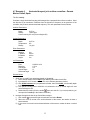
1.3 VISJET Main window layout
The Main components in the VISJET window:
The right panel is for data input. The left panel is for the 3D graphic output or Outfall View. The top
part of the middle panel shows the projection on the cutting plane. The lower part provides the
numerical results of the simulation. The toolbox allows the user to manipulate the view of the
graphic outputs and the cutting plane.
3
1.4 Notes on system requirements for using VISJET 2.0
1. 3D visualization is quite resource demanding, so users need to have suitable computer
hardware for running VISJET 2.0 with satisfactory performance.
2. The minimum system requirements are:
•
•
•
•
•
•
3
Pentium II 400 MHz
128 MB RAM
100 MB free hard-disk space
Windows 98 SE, ME, NT 4.0, 2000 and XP
Screen resolution 1024 x 768 supporting 16-bit high colour
3D graphics board with 4 MB memory
To ensure a reasonable performance, some of the special virtual reality features, such as the
disturbance of the water surface and the more realistic atmosphere representation, are turned
off by default if your system only satisfies the minimum requirements.
4. To run VISJET 2.0 with all the special visualization features switched on, it is recommended
that your system should have:
• Pentium III 1 GHz
• 256 MB RAM
• 3D graphics board with 16 MB memory
5. Running VISJET 2.0 will take up at least 20 MB memory. More memory will be used up when
greater number of jets is modeled (for 20 jets, 39 MB memory will be occupied). Also,
displaying the cut plane will require much more memory during the creation process (for 20
jets, 80 MB memory is needed at the peak). Therefore, when working with a large number of
jets, users should make sure that sufficient memory is available. In most cases, the user will
probably be working with less than 20 jets.
6. The VISJET file with an extension vj has a minimum size of about 100 KB. With 20 jets, the file
size will increase up to about 3 MB.
7. For Windows 98 users, they should set their colours to 16-bit high colour. Using 24-bit true
colour may cause VISJET failure to display the 3D graphics window.
4
2. JETLAG
2.1 JETLAG - Introduction
JETLAG is a robust LAGrangian JET model that handles an arbitrarily inclined round buoyant jet in
a current, with a three-dimensional trajectory. It uses a Lagrangian Projected Area Entrainment
(PAE) concept which assumes that the “forced entrainment” (the vortex entrainment in the
bent-over jet/plume) is equal to the ambient flow intercepted by the ‘windward’ face of the plume
element. The model has a rigorous theoretical basis, and its connection with Eulerian models can
be established; it is consistent with the concept of asymptotic flow regimes (e.g. the advected puff
and thermal in the bent-over phase).
JETLAG is unique in that the Lagrangian model does not, strictly speaking, solve the usual Eulerian
governing differential equations of fluid motion and mass transport. Instead, the model simulates
the key physical processes expressed by the governing equations. The unknown jet trajectory is
viewed as a series of non-interfering “plume-elements” which increase in mass due to
shear-induced entrainment and vortex-entrainment (forced entrainment) due to the crossflow while rising by buoyant acceleration. The model tracks the evolution of the average properties of a
plume element at each step by conservation of horizontal and vertical momentum, conservation of
mass accounting for entrainment, and conservation of mass/heat - all in a fixed reference frame.
The vortex entrainment is accurately determined, while pressure drag is ignored. The approach can
also be shown to be equivalent to but more robust than the alternative of formulating and solving
the Eulerian governing equations in natural co-ordinates.
The model predictions have compared well with basic laboratory experimental data, and it displays
the correct asymptotic behaviour. JETLAG reproduces the correct behaviour of i) a round buoyant
jet in stagnant or near stagnant fluid, and ii) a line puff/impulse advecting at the ambient velocity, in
the bent-over phase, for momentum/buoyancy dominated jets. The current version of the model
has been validated against experimental data by different investigators for: straight jets and
plumes, vertical buoyant jet and dense plume in crossflow, oblique momentum jet in crossflow,
horizontal buoyant jet in coflow; horizontal buoyant jet in crossflow; vertical buoyant jet in stratified
crossflow; coflow and counterflowing momentum jets; buoyant plumes in weak current. The
detailed derivation of the model can be found in Lee and Cheung (1990); related studies and
verification can be found in the references provided at the end of the user guide.
5
2.2 The origin of JETLAG
JETLAG has its roots in the model UOUTPLM initially developed by the United States
Environmental Agency (Frick 1984; Muenlenhoff et. al 1985). It uses a Lagrangian Projected Area
Entrainment (PAE) concept to treat the buoyant jet in crossflow problem.
The model UOUTPLM has several important limitations: a) it can handle only jets with
two-dimensional trajectories (e.g. vertical jet in crossflow); b) the shear entrainment hypothesis is
incorrect; c) by virtue of the control volume formulation and the implementation of the entrainment
computation, the scheme can be unstable in regions of strong plume curvature; d) its connection
with basic jet theory has not been established, and e) the interpretation of the model predictions in
terms of the contaminant concentration field in the bent-over jet is not clear.
Hence a great number of practical outfall discharge problems cannot be handled by UOUTPLM; for
example, a horizontal buoyant jet in a crossflow, dense plumes, oblique jets, and jet in coflow or
counterflow. Many outfalls located in shallow coastal waters around the world (e.g. in SE Asia and
in the UK) fall into this category. The prediction of mixing for these outfalls cannot be satisfactorily
handled by the USEPA models. Even within the category of jets with two-dimensional trajectories,
the stated range of applicability for UOUTPLM is only VANG= -5° to 90°, where VANG is the initial
discharge angle from the horizontal. These significant limitations were removed in the newly
developed and considerably more powerful JETLAG (Lee and Cheung 1990; Cheung 1991;
Cheung and Lee 1996, 1999) which handles an arbitrarily-inclined round buoyant jet in a current,
with a three-dimensional trajectory. Since its inception around 1989 (Lee and Cheung 1990),
JETLAG has proved to be a robust model that has been applied and verified in many situations
(e.g. Cathers and Pierson 1991; Gordon and Fagan 1991; Horton et al 1997; see next section). The
model also includes a general formulation for jet mixing in a weak crossflow (the near-far field
transition), and has been validated against all available basic laboratory data, including jets issuing
into a counterflow (Chan and Lam 1998; Lam and Chan 1997).
Major advances in our understanding of jet/plume in crossflow have been made possible in recent
years with the development of non-intrusive laser-induced fluorescence (LIF) and digital image
processing techniques, and 2D/3D turbulence models (Chu et al 1996; Chen and Lee 2000; Lee,
Kuang and Chen 2002; Lee, Chen and Kuang 2002). These findings have been incorporated in the
current version of JETLAG. In particular, a novel treatment of the transition from the
jet/plume-dominated to the ambient current-dominated regime is included. The coflowing jet
situation has also been entirely re-modeled (Lee et al. 2000). These studies have also greatly
facilitated the interpretation of the Lagrangian model predictions in relation to the complex,
bifurcated scalar field in the bent-over phase of the buoyant jet.
6
2.3 List of JETLAG/VISJET Users and Prototype Outfall Applications
The Lagrangian model JETLAG/VISJET has been extensively validated against laboratory
experimental data of buoyant jets in a crossflow by many investigators. It has also been verified in
field experiments, and applied to a number of actual outfall studies. The users and applications
include:
Sydney Deepwater Ocean Outfall post-operation environmental monitoring study
Zarautz Marine Outfall, Spain
Shek O Outfall beach pollution study
Urmston Road Sewage Outfall (Northwest New Territories, Hong Kong) post-operation monitoring
study
Hong Kong Strategic Sewage Disposal Scheme (SSDS) Environmental Impact Assessment
Project
Shanghai Stage 2 Sewage Outfall
North Point Outfall
Hastings Outfall, Sidmouth outfall, Gosport outfall, Jaywick outfall (United Kingdom)
Stonecutters Island Interim Outfall, Harbour Area Treatment Scheme (HATS)
Bhabha Atomic Research Centre (Isotope Division), Trombay, India
List of Users
Academic Institutions
NATO Saclant Undersea Research Centre
OGI School of Science & Engineering
Rutgers University
Seoul National University
South China Sea Institute, China
The Department of Environmental Protection,
Australia
The Hong Kong Polytechnic University
The University of Hong Kong
The University of Queensland
Tianjin University
Tongji University
Tsinghua University
Universidade Do Porto
University of Alberta
University of Arizona
University of Canterbury
University of Hawaii
University of Karlruhe
University of Michigan
University of Southern California
University of Toronto
University of Wisconsin-Madison
Univ. Metropolitana, Venezuela
Alaska Department of Environmental
Conservation
British Columbia Government
California State Water Resources Control Board
City University of Hong Kong
Clarkson University
Duke University
Fisheries and Oceans Canada
Goddard Earth Sciences Technology
Center/NASA Goddard Space Flight Center
Hong Kong University of Science and
Technology
Indian Institute of Technology, Bombay
Iran University of Science and Technology
Korea Ocean Research and Development
Institute
Loughborough University
Massachusetts Institute of Technology
McGill University
Monterey Institute of International Studies
National Center for High-Performance
Computing, Taiwan
National Institute of Water & Atmospheric, New
Zealand
National Taiwan University
National Water Research Institute, Canada
7
Consulting Engineering Firms
Applied Science Associates, USA
Atkins China Ltd, HK
Battelle, USA
CDM International Inc.
CH2M HILL
Joiner Engineering
Montgomery Watsons HK Ltd.
Mott Connell Ltd., HK
Mouchel Asia Ltd, HK
Patterson Britton & Partners, Australia
Tetra Tech, Inc
Other Individual Users From
Australia
Brazil
Canada
Germany
Greece
India
Iran
Italy
Korea
New Zealand
Portugal
P. R. China
Taiwan, China
Saudi Arabia
United Kingdom
USA
Venezuela
8
2.4 Output file - SUSPEND
SUSPEND is a standard output file. Discharge parameters and characteristic length scales are also
printed in addition to the numerical results. The (x, y, z) co-ordinates of the computed jet trajectory
are printed along with the jet half-width, average dilution and velocity, and average density deficit.
9
2.5 References
Cathers, B. and Peirson, W.L. (1991). “Verification of plume models applied to deepwater outfalls”,
in Proceedings of the International Symposium on Environmental Hydraulics, Hong Kong, Lee,
J.H.W. and Cheung, Y.K. (ed.), December 1991, Vol.1, Balkema, pp.261-266.
Chan, C.H.C. and Lam, K.M. (1998), “Centreline velocity decay of a circular jet in a counterflowing
stream”, Physics of Fluids, Vol. 10 (3), pp. 637-644.
Chen, G.Q. and Lee, J.H.W. (2000). “Numerical experiment of two-dimensional line thermal”,
Journal of Hydrodynamics, Ser.A, Vol.15, No.4, pp.411-423.
Cheung, V. (1991) Mixing of a round buoyant jet in a current. Ph.D. thesis, Dept. of Civil &
Structural Engineering, University of Hong Kong, Hong Kong.
Cheung, V. and Lee, J.H.W. (1996) Discussion of “Improved prediction of bending plumes”. Journal
of Hydraulic Research, Vol.34, No.2, pp.260-262.
Cheung, V. and Lee, J.H.W. (1999) Discussion of “Simulation of oil spills from underwater
accidents I: model development”, Journal of Hydraulic Research, Vol.37, pp.425-429.
Chu, P.C.K. and Lee, J.H.W. (1996). “Mixing of a bent-over jet in crossflow”, Proc. 11th ASCE
Engineering Mechanics Specialty Conference, Fort Lauderdale, Florida, May 1996, pp. 910-913.
Chu, P.C.K., Lee, J.H.W., and Chu, V.H. (1999). “Spreading of a turbulent round jet in coflow”,
Journal of Hydraulic Engineering, ASCE, Vol.125, No.2, pp.193-204.
Chu, V.H. and Goldberg, M.B. (1974) “Buoyant forced plumes in crossflow”, J. Hydraulics Div.,
ASCE, Vol.100, HY9, pp.1203-1214.
Chu, V.H. (1977). “A line impulse model for buoyant jets in a crossflow”, in Heat Transfer and
Turbulent Buoyant Convection (Spalding, D.B. ed.), Hemisphere, Washington D.C., Vol.1,
pp.625-636.
Chu, V. H. (1994) “Lagrangian scalings of jets and plumes with dominant eddies,” in Recent
Research Advances in the Fluid Mechanics of Turbulent Jets and Plumes, NATO ASI Series E:
Applied Sciences, Vol. 255, (Davies, P.A. and Valente Neves, M.J., eds.), Kluwer Academic
Publishers, Dordrecht, pp. 45-72.
Chu, V.H. and Lee, J.H.W. (1996). “A general integral formulation of turbulent buoyant jets in
crossflow”, Journal of Hydraulic Engineering, ASCE, Vol. 122, No.1, pp. 27-34.
Fischer, H. B., etal (1979) Mixing in Inland and Coastal Waters, Academic Press, San Diego,
California.
Frick, W.E. (1984) Non-empirical closure of the plume equations. Atmospheric Environment,
Vol.18, No.4, pp. 653-662.
Gordon, A.D. and Fagan, P.W. (1991). “Ocean outfall performance monitoring”, in Proceedings of
the International Symposium on Environmental Hydraulics, Hong Kong, Lee, J.H.W. and Cheung,
Y.K. (ed.), December 1991, Vol.1, Balkema, pp.243-248.
Horton, P.R., Lee, J.H.W. and Wilson J.R. (1997). “Near-field JETLAG modelling of the Northwest
New Territories Sewage Outfall, Urmston Road, Hong Kong”, Proc. 13th Australasian Coastal and
Ocean Engineering Conference (Pacific Coasts and Ports '97), Christchurch, New Zealand, Sept.
97, Vol.2, pp. 561-566.
10
Lam, K.M. and Chan, H.C. (1997), “Round jet in ambient counterflowing stream”, Journal of
Hydraulic Engineering, ASCE, Vol. 123 (10), pp.895-903.
Lee, J.H.W. and Neville-Jones, P. (1987). “Initial dilution of horizontal jet in crossflow”, Journal of
Hydraulic Engineering, ASCE, Vol.113, HY5, pp.615-629.
Lee, J.H.W. and Neville-Jones, P. (1987). “Design of sea outfalls - Prediction of initial dilution and
plume geometry”, Proceedings of the Institution of Civil Engineers, Part 1, [Design and
Construction], Vol.82, pp. 981-994.
Lee, J.H.W. and Cheung, V. (1990) Generalized Lagrangian model for buoyant jets in current.
Journal of Environmental Engineering, ASCE, 116(6), 1085-1105.
Lee, J. H. W. and Chu, P. C. K. (1995) “Application of video image processing in the study of
environmental flows”, Proc. 10th ASCE Engineering Mechanics Conference, University of
Colorado, Boulder, Vol.2, pp. 1014-1017.
Lee, J.H.W. Rodi, W. & Wong, C.F. (1996). "Turbulent line momentum puffs." Journal of
Engineering Mechanics, ASCE, 122, 19-29.
Lee, J.H.W. and Chu, P.C.K., ``On the added mass of a turbulent jet in crossflow'', Proc. 27th IAHR
Congress, August 1997, San Francisco, Vol.1 ({\it Environmental and coastal hydraulics}), pp.
269-274.
Lee, J.H.W. and G.Q. Chen, “The jet in crossflow and the puff analogy'', Proc. 12th ASCE
Engineering Mechanics Conference, La Jolla, California, May 17-20, 1998 (H.Murakami and
J.E.Luco Ed.), pp. 1792-1795.
Lee, J.H.W., Li, L., and Cheung, V. (1999). “A semi-analytical self-similar solution of a bent-over jet
in crossflow”, Journal of Engineering Mechanics, ASCE, Vol.125, pp.733-746.
Lee, J.H.W., Cheung, V., Wang, W.P., and Cheung, S.K.B., ``Lagrangian modeling and
visualization of rosette outfall plumes'', Proc. Hydroinformatics 2000, Iowa, July 23-27, 2000
(CDROM)
Lee, J.H.W., Kuang, C.P., and Chen, G.Q. (2002). “The structure of a turbulent jet in crossflow effect of jet-to-crossflow velocity”, China Ocean Engineering, Vol.16, No.1, pp.1-20.
Lee, J.H.W., Chen, G.Q., and Kuang, C.P. (2002). “Mixing of a turbulent jet in crossflow - the
advected line puff”, in Environmental Fluid Mechanics: theories and applications (Ed. H. Shen et
al), American Society of Civil Engineers (in press).
Muellenhoff, W.P. et al. (1985) Initial mixing characteristics of municipal ocean discharges. Report
EPA-600/3-85-073, USEPA, Newport, Oregon.
Schatzmann, M. (1981) “Mathematical modeling of submerged discharges into coastal waters,"
Proc. 19th IAHR Congress, New Delhi, Vol. 3, pp. 239-246.
Wood, I. R. (1993) “Asymptotic solutions and behaviour of outfall plumes,” J. Hydr. Eng., ASCE,
Vol. 119, pp. 555-580.
Wright, S.J. (1977) "Effects of ambient crossflow and density stratification on the characteristic
behavior of round turbulent buoyant jets," Report No. KH-R-36, W.M. Keck Lab. of Hydr. and Water
Resour., California Inst. of Tech., Pasadena, Calif.
11
3. User Interface
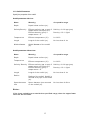
3.1 Input parameters
3.1.1 Ambient parameters
Specify the vertical structure of the ambient water:
N a me
Me a n in g
A c cep t ab le ra nge
D e p th
D e p th b el ow s ur f ace ( m ) .
Sa li ni ty /De nsi ty
Ambien t salinity ( pp t or ps u) if
t e mpe r a ture no t e qua l t o 0 ;
Ambien t d ens ity (g /ml) if
t e mpe r a ture = 0 .
S a li ni t y : 0~1 00 p p t
(ps u)
T e mpera ture
Ambien t temper a ture ( ºC) .
0~ 100 ºC
Cur rent
H or iz o n ta l c ur r en t s pee d ( m /s)
( as s um in g i n th e x-d ir ec t io n) .
De nsity: 0 .5~ 1 .5g /ml
No tes:
Only stable ambient stratification is allowed, i.e. ρ a ( d i ) ≤ ρ a ( d j ) if d i ≤ d j. ( d=de pt h
b e low free s urf ace ) .
12
3.1.2 Outfall Parameters
Specify the properties of the outfall:
Outfall parameters with riser:
N a me
Me a n in g
D e p th
D e p th b el ow s ur f ace ( m ) .
Sa linity /D ens ity
Effluen t sa lin i ty (p p t or psu) if
t e mpe r a ture no t e qua l t o 0 ;
Effluen t dens ity (g /ml) if
t e mpe r a ture = 0 .
S a li ni t y : 0~1 00 p p t ( ps u)
T e mpera ture
Effluen t temper a ture ( ºC) .
0~ 100 ºC
L eng th
Length of the outfall (m).
No less than 0.1m
W id th / diameter
W id th / diameter o f t he o u t fa ll
( m) .
Ac cep tab le ra nge
De nsity: 0 .5~ 1 .5g /ml
Outfall parameters without riser:
N a me
Me a n in g
D e p th
D e p th b el ow s ur f ace ( m ) .
T e mpera ture
Effluen t temper a ture ( ºC) .
0~ 100 ºC
Sa linity / De nsity
Effluen t sa lin i ty (p p t or psu) if
t e mpe r a ture no t e qua l t o 0 ;
Effluen t dens ity (g /ml) if
t e mpe r a ture = 0 .
S a li ni t y : 0~1 00 p p t ( ps u)
L eng th
Length of the outfall (m).
No less than 0.1m
Ra dius
R a di us o f th e o u t fal l . O u t fa ll is
d e fi ned as a p ip e in thi s mod e
( m) .
S pac e be twe en
J e ts
Spac e be twe en je ts moun ted
o n the ou t fa l l ( m) .
A c cep t ab le ra nge
De nsity: 0 .5~ 1 .5g /ml
No less than 0 .00 1m
Notes:
I f t he i np ut va r i ab le s a re out s id e t h e s pec if i ed ra ng e , t h en t h e u pp er / low er
limit w ill be assumed.
13
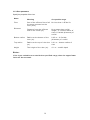
3.1.3 Riser parameters
Specify the properties of the riser:
N a me
Me a n in g
A c cep t ab le ra nge
F low
S u m o f t he e f f lu en t fl ow o f a ll
t h e por ts mo un te d on th e
r iser ( m³/s ).
No less than 1.0E-8m³/s
D is tanc e
D is tanc e fro m the o f fsh or e
e nd o f t he o u t fa ll ( m) .
No grea ter th an o u tfa ll
l en g th - 2 * b o t tom r ad ius o f
r is er - 0 .5 *w i d th ( d ia met er ) o f
o u t fa ll
Bo tto m ra dius
R a di us a t th e bo t t om o f t he
r iser ( m) .
0 . 05 m ~ 0 .5 *w i d th
( d i a m e t e r ) o f o u t fa l l
T op r ad ius
R a di us a t th e top o f th e r is er
( m) .
0 .01 m ~ bo ttom r ad ius o f
r iser
H e ig h t
T he h ei gh t o f t he r is er ( m) .
0 . 1 m ~ o u tf a l l de p th
Notes:
I f t he i np ut va r i ab le s a re out s id e t h e s pec if i ed ra ng e , t h en t h e u pp er / low er
limit w ill be assumed.
14
3.1.4 Jet parameters
Specify the properties of the jet:
N a me
Me a n in g
A c cep t ab le ra nge
F low
E f f l u e n t f l o w fro m th e p o r t
( m 3 /s) .
N o les s th an 1 .0 E- 8 m³/ s
D ia me ter
Por t diameter (m) .
No less than 1.0E-4m
Port Height
P or t he igh t ( m) .
No grea ter th an r iser
h ei gh t
V er t ica l a ng le
V er t ica l je t d is c h arge a ng le
r e la t i ve t o H or iz o n ta l p la ne ( 90 º
f or a ver t ica l p or t) .
H or iz o n ta l a ng le
H or iz o n ta l a ng le o f c ur r en t
direc tion with res pec t to jet
d isch arge (9 0º fo r a
p er pe nd ic ul ar c r oss fl ow ) .
Sa linity / De nsity
E f f l u e n t s a l i n i t y ( p p t) i f
t e mpe r a ture no t e qua l t o 0 ;
Effluen t dens ity (g /ml) if
t e mpe r a ture = 0 . (Read on ly)
S a li ni t y : 0~1 00 p p t
Effluen t temper a ture
( ºC) . (Re ad o nly)
0~ 100 ºC
T e mpera ture
De nsity: 0 .5~ 1 .5g /ml
Notes:
I f t he i np ut va r i ab le s a re out s id e t h e s pec if i ed ra ng e , t h en t h e u pp er / low er
limit w ill be assumed.
15
3.1.5 Cutting plane parameters
A cutting plane in VISJET is defined by its normal vector. The orientation of the normal vector is
defined by the vertical and horizontal angle (as in the JETLAG model); refer to ``How To’’ under
``Startup Tips’’. The control parameters for the cutting plane:
V er t ica l a ng le
H or iz o n ta l a ng le
D is tanc e
T he an gle o f th e nor ma l vec tor o f the cu ttin g p lan e r ela tive
to hor izon ta l p la ne (90 º for a hor izon tal plan e ; 0º for
v er t ica l p lan e)
T he an gle b e twee n the pr ojec tion o f th e n or ma l vec tor on
th e hor izonta l p lan e an d the flow d irec tio n ( x-a xis) ( 90º for
a v er t ica l s ec t io n - s ide v iew , an d 0 º fo r a v er t ica l s ec t io n,
cross -sec tion vi ew)
D is tanc e fro m the disch arge po in t (N o gr eater than 25
times of water depth).
16
3.2 Output parameters
3.2.1 Key parameters and length scales
The following are the key parameters and length scales for each jet:
Depth.
Diameter
Uj
Ua
Dρ/ρa
ρj
ρa
Ver. Ang
Hor. Ang
Fd
Qj
Mj
Bj
lQ
lm
lb
lM
Sm
Sb
Port depth (m)
Port diameter D (m)
Initial jet velocity, Uj (m/s)
Ambient current velocity, Ua (m/s)
Dimensionless initial density difference, (ρa(0)-ρj)/ρa(0)
Initial effluent density (g/ml)
Ambient density at source level, ρa(0) (g/ml)
Vertical discharge angle, Φj (degree)
Horizontal discharge angle; θj (degree)
Jet Densimetric Froude no., F = Vj/(gD(ρa(0)-ρj)/ρa(0))1/2
Volume flux / discharge flow, Q = Vj (πD2/4) (m3/s)
Momentum flux, M = Vj2(πD2/4) (m4/s2)
Buoyancy flux = Qg(ρa(0)-ρj)/ρa(0) (m4/s3)
Discharge (volume, geometric) length scale, lQ = Q/M1/2 (m)
Cross momentum length scale, lm = M1/2/Ua (m)
Cross buoyancy length scale, lb = B/Ua3 (m)
Jet/plume length scale, lM = M3/4/B1/2 (m)
Characteristic dilution for momentum dominated far field
(mdff), Sm = Ua lm2/Q
Characteristic dilution for buoyancy dominated far field
(bdff) , Sb = Ua lb2/Q
3.2.2 Disk information
The following information about the computed disk will be displayed:
Disk no.
Centre position
Radius
Thickness
Angle
Velocity
Concentration
The sequence no. of the selected computed
disks for the selected jet
The (x, y, z) co-ordinates of the center of the
selected disk, which is the computed jet trajectory
Jet half width of the selected disk
Thickness of the selected disk
Vertical angle is the angle between the jet axis
and the horizontal plane; horizontal angle is the
angle between the x-axis and the projection of
the jet axis on the horizontal plane
Jet velocity of the selected disk
Maximum/average concentration of the selected
disk
17
3.2.3 Cross section concentration
The following information related to the cross section concentration will be displayed:
Position
Concentration
The (x, y, z) co-ordinates at the position of the
point selected by the mouse or pointing device
Average concentration at the above position
3.2.4 Cross section area information
The following information related to the projected area of the jets will be displayed:
Total area
Sum of areas
Selected jet area
Horizontal span
Vertical span
The total projected area of the jets on the cutting
plane; the overlapped areas are not double
counted
The sum of all the projected areas of the
individual jets
The projected area of the selected jet
The horizontal span of the projected region for
the selected jet (defined by bounding box)
The vertical span of the projected region for the
selected jet
18
4. Tutorial Examples
4.1 Example 1
Vertical buoyant jet in stagnant fluid
4.2 Laboratory Example
Wah Fu Outfall Discharge
4.3 Example 2
Horizontal buoyant jet in stagnant stratified fluid
4.4 Example 3
Multiple buoyant jets in stagnant fluid
4.5 Example 4
Vertical buoyant jet in stratified crossflow
4.6 Example 5
Vertical dense jet in uniform crossflow
4.7 Example 6
Horizontal buoyant jet in uniform crossflow - Zarautz Marine Outfall, Spain
4.8 Example 7
Horizontal buoyant jet in stratified crossflow - Zarautz Marine Outfall, Spain
4.9 Example 8
Buoyant jets from a rosette-shaped ocean outfall riser in natural flow –Hong Kong Strategic
Sewage Disposal Scheme (SSDS)
19
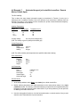
4.1 Example 1
Vertical buoyant jet in stagnant fluid
The file is tut1.vj.
VISJET simulates the mixing of single or multiple buoyant jets discharged from one or more risers
mounted on an ocean outfall. In a particular application, the input parameters for the ambient
condition, the outfall, riser, and jet characteristics are needed. For example, a single buoyant jet
can be simulated by specifying a single jet on a single riser. Multiple jets can be simulated by
specifying a single jet on each of a number of risers. Rosette jet groups on multiple risers can be
simulated by specifying the multiple jet characteristics on each of the risers. We start with several
examples on how to use VISJET for simulating a single buoyant plume, which is of interest in many
applications, followed by more complicated situations.
The first example is for a single vertical buoyant jet discharge into an otherwise stagnant fluid. For
a single jet the riser flow is the same as the jet flow. The main parameters are as follows:
Ambient Parameters:
Depth
20 m
Density
1.0256 g/ml
Current velocity 0.0 m/s (Current angle 90º)
Outfall Parameters:
Depth
Temperature
Density
22 m
0ºC
1.0 g/ml
(The density of the effluent is entered as input. There are two possible formats:
i) if density is input directly, a zero value, 0.0, must be entered for temperature;
ii) alternatively, both the temperature and salinity of the effluent can be entered as input and
the effluent density will then be computed by the model.
Riser Parameters:
Distance
T. Radius
B. Radius
Height
0m
0.05 m
0.05 m
2m
(For single jet the riser distance is immaterial; set to zero)
Jet Parameters:
Flow
Diameter
Port height
Vertical angle
Horizontal angle
0.03 m³/s
0.1 m
2m
90º
0º
General Notes:
1. Study how to input parameters.
i) Click New in the startup tips window.
ii) Click Add a level twice, input ambient parameters as shown above.
20
iii) Click Next, select Create a scenario with riser. Then click Create an outfall, and click
Outfall_1, and input the above outfall parameters.
iv) Click Riser1, input the above riser parameters.
v) Click Jet1, input the above jet parameters.
vi) Click Finish
If you have problems with the input parameters, you can open the file tut1.vj in the folder
tutorial files to examine the correct input parameters (Click Outfall_1, Riser_1, and Jet_1 to
observe the input parameters).
2. Use the animation function to see the evolution and spread of the jet. Click toolbar
to see
the rise and growth of the jet from the discharge port to water surface. In the Lagrangian model,
the jet path is made up of a series of plume elements (`disks’) which vary in position, width, and
velocity as they mix with the surrounding fluid.
3. Study how to get the jet characteristics of each Lagrangian element: information about the
computed average velocity, maximum concentration, and average dilution at that height.
i) Select toolbar or press the right mouse button and select Pick.
ii) Put cursor at any point on the jet you want to get the information in the data output window.
iii) Move scroll bar up or down at the right of the data output window to choose the disk
number. For example, the center of Disk 46# is located at (0, 0, 0.11), visual radius = 0.048
m, thickness = 0.037 m, vertical angle = 90º, horizontal angle = 0º, average velocity = 2.8
m/s, maximum concentration = 1.0, average dilution = 1.4 and average concentration =
0.7332.
The dilution is a measure of the degree of mixing achieved by the jet; the inverse of
dilution is the relative concentration of any pollutant contained in the discharge.
4. Save file: you can select Save as in main menu File to save the file (file format ∗∗∗.vj) for later
reuse or modification.
5. Compute a horizontal buoyant jet in stagnant fluid based on this case. You just need to
change the vertical angle 90º to 0º in the input jet parameters, resimulate the model (Click the
toolbar
then save this example. If you have problems, you can open the file tut1a.vj in the
folder tutorial files). Notice the dilution is increased for this jet as the length of the jet path is
greater than that of the vertical jet at the same vertical position. For example, Disk 296#, the
disk center is located at (2.03, 0, 0.11), visual radius = 0.27 m, thickness = 0.0066 m, vertical
angle = 8.4º, horizontal angle = 0, average velocity = 0.50 m/s, maximum concentration = 0.226
and average dilution = 7.5.
6. You can also predict the jet from an actual outfall and compare it with observations in a
laboratory experiment!
7. You can also try the “Create a scenario without riser” at 1.iii)
8. Close this file to start next tutorial.
21
4.2 Laboratory Example Wah Fu Outfall Discharge
The file is WahFu.vj.
Consider the Wah Fu Outfall which discharges domestic wastewater from a housing estate in the
form of a number of submerged buoyant jets, at a depth of about 7-12 m. The jets are sufficiently
spaced apart so that they may be considered independent of each other. In this development, salt
water is used for flushing, so that the jet discharge is brackish water (i.e. a mixture of sea water and
freshwater). Compute the mixing for this discharge which is inclined at 20 degrees to the
horizontal, and compare your computed results with the corresponding observed jet in a laboratory
experiment. The main parameters are as follows:
Ambient parameters:
Depth below surface (m)
Density (Sigma-t)
0
18.0
7
18.0
Current velocity
0.0 m/s (Current Angle=90º)
or
Density (g/ml)
1.018
1.018
(N.B. density (g/ml) = 1. + 0.001 Sigma-t)
Outfall parameters:
Depth
Density
9.0m
1.004 g/ml (Sigma-t = 4 unit)
Riser Parameters:
Distance
T. Radius
B. Radius
Height
0m
0.05m
0.05m
2m
Jet Parameters:
Flow
Diameter
Port height
Vertical angle
Horizontal angle
0.00626 m³/s
0.1 m
2m
20º
0º
General Notes:
1. Animate the jet evolution and compare the computed results with the corresponding observed
jet in a laboratory experiment. Note the irregular edge of the real turbulent jet; the model
computes only the average turbulent-mean properties.
2. Click View suspend file (More info in data output window) to see the printout of the computed
results in a SUSPEND file.
3. The SUSPEND file shows key input parameters and length scales that govern the mechanics
of buoyant jet mixing. For example, Total Q = 0.00626 (m³/s), jet velocity = 0.8 m/s, Jet
densimetric Froude number Fd =6.86.
22
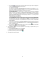
4. The following is the observed dyed jet of the Wah Fu outfall discharge; in this experiment the jet
is a 1:11 scale model of the actual outfall, discharged at the same jet densimetric Froude
number of 6.8.
23
4.3 Example 2
Horizontal buoyant jet in stagnant stratified fluid
The file is tut2.vj.
The ambient receiving water often has a vertical variation of salinity and/or temperature, leading to
density stratification. The jet may cause so much mixing that the mixed effluent stays trapped below
the free surface. In this example we compute the mixing for a horizontal buoyant jet in a stratified
fluid. The main parameters are as follows:
Ambient Parameters:
Depth below surface (m)
0
1
4
7
10
13
16
19
20
Density (Sigma-t)
8.0
8.4
11.0
12.2
13.2
15.3
16.5
16.6
16.6
Density (g/ml)
1.008
1.0084
1.011
1.0122
1.0132
1.0153
1.0165
1.0166
1.0166
(N.B. Density (g/ml) = 1 + 0.001 Sigma-t)
Current velocity
0.0 m/s (Current Angle =90º)
Outfall Parameters:
Depth
Temperature
Density
22 m
0ºC
0.999 g/ml (Sigma-t = -1 unit)
Riser Parameters:
Distance
T. Radius
B. Radius
Height
0m
0.05 m
0.05 m
2m
Jet Parameters:
Flow
Diameter
Port height
Vertical angle
Horizontal angle
0.0147 m³/s
0.125 m
2m
0º
0º
General Notes:
1. Click Open in the startup tips window, then select and open file tut2.vj in the folder tutorial files
2. The density variation of the ambient fluid can be specified in either of the following two ways: i)
the salinity and temperature at each depth are entered, from which the density will be
computed by the model by the equation of state; ii) the density is given directly in units of ρ
(g/ml) – for this case the density is entered under the Salinity column in ambient parameter
24
window, and a zero (0.0) value must be entered for temperature. For this case the natural
density stratification is represented by values given at 8 depths.
3. Animate the jet evolution and observe how the jet is trapped beneath the water surface. Click
View suspend file (More info in data output window) to see the printout of the computed
results in a SUSPEND file.
4. The SUSPEND file shows key input parameters and length scales that govern the mechanics
of buoyant jet mixing. For example, Total Q = 0.0147 (m³/s), Densimetric Froude number Fd
=8.22, Buoyancy flux Bj = 0.0025 m4/s², jet momentum length scale lM = 0.97, and so on. The
computed jet characteristics (co-ordinates of the jet trajectory, plume visual radius, velocity,
concentration, dilution etc.) are tabulated. You will find some information about trap level. For
this case, the neutral buoyancy level = 5.1 m, with a corresponding average dilution = 38.1
and visual radius = 1.14 m; the buoyant jet center maximum rise height = 7.1 m,
corresponding average dilution = 41.1 and visual radius = 2.58 m.
5. In the summer wet season, the receiving water is often stratified, and the sewage field may not
reach the surface; the submergence of the sewage may be desirable for protection of nearby
beaches.
Notice that the computation can continue after the first trap level; the computation will be
stopped after the first oscillation in VISJET, at trapped level = 5.41 m, corresponding average
dilution = 53.9 and visual radius = 1.61 m.
6. Close this file to start next tutorial, or change input parameters to make your own run.
25
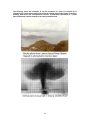
The following shows two examples of real life examples of a plume or buoyant jet in
stagnant fluid: i) the trapped smoke plume from the Lamma Island power station in the early
morning, when there was a temperature inversion. ii) laboratory experiments of a plane
(two-dimensional) vertical buoyant jet in linearly stratified fluid.
\
26
4.4 Example 3
Multiple buoyant jets in stagnant fluid
The file is tut3.vj.
Consider the horizontal buoyant jet example in Tutorial 1 again, but this time instead of using one
jet, divide the flow of 0.03 m³/s into 4 jets, each discharged from a different riser. So now we have
FOUR horizontal buoyant jets in a uniform stagnant fluid, but each port discharges ¼ of the original
flow. The main parameters are as follows:
Ambient Parameters:
Depth
20 m
Density
1.0256 g/ml
Current velocity 0.0 m/s (Current Angle=90º)
Outfall Parameters:
Depth
Temperature
Density
22 m
0ºC
1.0 g/ml
Riser Parameters:
Distance
T. Radius
B. Radius
Height
0 m (riser1)
20 m (riser2)
40 m (riser3)
60 m (riser4)
0.05 m
0.05 m
2m
(The distance from the most offshore end riser is indicated above; the spacing between two
adjacent risers is 20 m).
Jet Parameters:
Flow
Diameter
Port height
Vertical angle
Horizontal angle
0.0075 m³/s
0.1 m
2m
0º
0º
General Notes:
1. You can also change the orientation of the diffuser axis with respect to the current by changing
the default current angle 90o in the ambient parameter window.
2. Click Open in the startup tips window, then select and open file tut3a.vj in the folder tutorial
files
3. Do the following to add three new risers with one jet on each riser:
i) Highlight Riser1, click Add, riser2 and the jet from this riser will be created.
ii) Highlight the new riser and its jet1, input the corresponding parameters, then specification
of the riser and the associated jet will be completed.
27
iii) Repeat the procedure to create other two risers and their associated jets. Resimulate the
model (Click the toolbar , then save this file). Use the animation function (Click the
toolbar ) to see the evolution and spread of the jets.
If you have any problems, you can consult tut3.vj to look up the correct input parameters.
4. Open the SUSPEND file (Click View suspend file in menu More info in Data output window)
to see the results and determine the dilution for this case of multiple jets. You will find that each
jet achieves an average dilution at water surface = 397; the water quality is significantly
improved by this design compared with the case in tutorial 1 (average dilution = 213).
5. When will the plumes from adjacent risers merge? Decrease the distance between risers to
find the pattern of plume interaction.
6. Close this file to start the next tutorial or change parameter values to create your own run.
28
4.5 Example 4
Vertical buoyant jet in stratified crossflow
The file is tut4.vj.
Consider a single vertical discharge into a horizontal crossflow of ua=0.1 m/s, at a depth of 14 m
below the free surface. The receiving water is linearly stratified. The main parameters are as
follows:
Ambient Parameters:
Depth below surface (m)
Density (Sigma-t)
0.0
14.0
22.9
25.0
Current velocity 0.1 m/s (Current Angle=90º)
Outfall Parameters:
Depth
Temperature
Density
16 m
0ºC
1 g/ml
Riser Parameters:
Distance
T. Radius
B. Radius
Height
20 m
0.05 m
0.05 m
2m
Jet Parameters:
Flow
Diameter
Port height
Vertical angle
Horizontal angle
0.0147 m³/s
0.1 m
2m
90º
0º
General Notes:
1. Click Open in the startup tips window, then select and open file tut4.vj in the folder tutorial files
2. Animate the jet (Click the toolbar ) evolution and observe how the jet is bent over into a
trapped submerged layer. Click View suspend file (in menu More info in Data output window)
to see the printout of the computed results in a SUSPEND file.
3. In the SUSPEND file, you will find some information about trap level. For this case, the neutral
buoyancy level = 4.85 m, with a corresponding average dilution = 123.3; the buoyant jet
center maximum rise height = 5.86 m, corresponding average dilution = 225.4. The
computation will be stopped at trapped level = 5.16 m, with corresponding average dilution =
274.
4. Click Key parameters and length scales (in menu More Info in Data output window) to see
key input parameters and length scales that govern the mechanics of buoyant jet mixing. For
example, discharge length scale lQ = 0.089 m, momentum length scale lm = 1.66 m, Buoyancy
29
length scale lb = 3.52 m, jet/plume length scale lM = 1.14 m, characteristic dilution for
momentum dominated far field Sm = 18.7 and for buoyancy dominated far field Sb = 84.1.
5. Observe what happens when the ambient current is increased to 0.3 m/s. Input 0.3 under the
Current column in ambient window, resimulate the model (Click the toolbar , then save this
file. If you have problems, you can open the file tut4a.vj in the folder tutorial files). You will find
the sewage will be more trapped as shown in screen figure or from SUSPEND file. In this case,
trapped level = 2.93 m, with corresponding average dilution = 390.7.
6. Compute a vertical buoyant jet in uniform crossflow based on this case. You just need to
change density to 1.025 at depth = 0 m in the input jet parameters, resimulate the model (Click
the toolbar , then save this file. If you have problems, you can open the file tut4b.vj in the
folder tutorial files). For this case, you will find that the sewage plume will not be trapped and
reach the free surface.
8. Close this file to start the next tutorial, or change the parameter values to create your own run.
30
4.6 Example 5
Vertical dense jet in uniform cross flow
The file is tut5.vj.
Consider a single vertical dense jet discharged into a uniform crossflow. In some applications the
jet or plume discharge is negatively buoyant – i.e. the effluent discharge is heavier than the ambient
fluid (e.g. concentrated brine discharge from desalination plants). The main parameters are as
follows:
Ambient Parameters:
Depth
40 m
Density
0.9756 g/ml
Current velocity 0.2 m/s (Current Angle=90º)
Outfall Parameters:
Depth
Temperature
Density
22 m
0ºC
1 g/ml
Riser Parameters:
Distance
T. Radius
B. Radius
Height
0m
0.05 m
0.05 m
2m
Jet Parameters:
Flow
Diameter
Port height
Vertical angle
Horizontal angle
0.03 m³/s
0.1 m
2m
90º
0º
General Notes
1. Study how to modify input parameter based on file tut1.vj.
i) At the startup window, select Open, open tut1.vj in the folder tutorial files.
ii) Modify depth to 40 m and ambient density to 0.9756 g/ml, current to 0.2 m/s in ambient
parameter window and flow to 0.03 m³/s in jet parameters window.
iii) Resimulate the model (Click the toolbar
, save this file. If you have problems, you can
open the file tut5.vj in the folder tutorial files).
For this case, the ambient density ρa = 0.9756 g/ml is less than the jet density ρj = 1g/ml, it is a
negatively buoyant discharge. On the screen, you will see the dense plume first moves
upwards due to its initial momentum, reaches a maximum height, and then bends downwards
to reach the seabed.
2. Open the SUSPEND file (Click View suspend file in menu More info in Data output window)
to see the computed results: the buoyant jet center maximum rise height = 2.69 m and
corresponding average dilution = 43.9. Plume hits the seabed (z = -20.0 m) with average
dilution = 4865.
31
3. Click Disk in Data output window, the information on the Lagrangian elements (disks) is shown.
For example, the disk 703# located at (8.3557, 0, 1.288) has the following properties: visual
radius = 1.50 m, thickness = 0.0027 m, vertical angle = -19.6º, horizontal angle = 0, average
velocity = 0.21 m/s, maximum concentration = 0.022, average dilution = 98.6 and average
concentration=0.0101.
4. Close this file to start the next tutorial.
32
4.7 Example 6
Horizontal buoyant jet in uniform crossflow -Zarautz
Marine Outfall, Spain
The file is tut6.vj
Consider a single horizontal buoyant jet discharged into a perpendicular uniform crossflow. Since
the direction of jet momentum is different from the direction of buoyancy in the presence of the
crossflow, the jet has a three-dimensional trajectory. The main parameters are as follows:
Ambient Parameters:
Depth
32.75 m
Density
1.0256 g/ml
Current velocity 0.2 m/s (Current Angle=90º)
Outfall Parameters:
Depth
Temperature
Density
34.75 m
0ºC
1.0 g/ml
Riser Parameters:
Distance
T. Radius
B. Radius
Height
0m
0.05 m
0.05 m
2m
Jet Parameters:
Flow
Diameter
Port height
Vertical angle
Horizontal angle
0.025221 m³/s
0.12 m
2m
0º
90º
General Notes:
1. Study how to modify input parameter based on file tut1.vj.
i) At the startup window, Select Open, open tut1.vj in the folder tutorial files.
ii) Input depth to 32.75 m and current to 0.2 m/s in ambient parameter window.
iii) Click Outfall structure in input parameter window, then click Outfall_1 and modify depth
to 34.75 m.
iv) Click jet1 and change flow to 0.025221 m³/s, diameter to 0.12 m, vertical angle to 0º and
horizontal angle to 90º.
v) Resimulate the model (Click the toolbar , then save this file. If you have problems, you
can open the file tut6.vj in the folder tutorial files).
2. Navigate through and view the jet from different angles.
i) Click toolbar
or press the right mouse button and select Rotate.
ii) When the cursor is moved in the vertical direction of the screen, the rotation is about a
horizontal axis.
iii) If the cursor is moved in the horizontal direction of the screen, rotation is about a vertical
axis.
33
3. Zoom and move screen figure.
i) Click the toolbar
or press the right mouse button and select Zoom. By moving the
cursor upward, you can zoom out from the current setting. By moving the cursor downward,
you can zoom in towards the center of current setting.
ii) Click the toolbar
or press the right mouse button and select Move. Press the mouse left
button, you can move the viewing window up, down, left and right.
4. Use the animation particle function to see the evolution and spread of the jet as well as how the
velocity changes as the plume comes up to the surface. Click the toolbar
to see the
evolution and spread of plume from the jet port to water surface.
5. Close this file to start the next tutorial.
34
4.8 Example 7
Horizontal buoyant jet in stratified crossflow -Zarautz
Marine Outfall, Spain
The file is tut7.vj.
This is about the same single horizontal buoyant jet considered in Tutorial 6, but the jet is
discharged into a stratified crossflow. Since the direction of jet momentum is different from the
direction of buoyancy in the presence of the crossflow, the jet has a three-dimensional trajectory.
The main parameters are as follows:
Ambient Parameters:
Depth (m)
Salinity (ppt)
0
15
32.75
Temperature (ºC)
15
22
34
30
25
20
Current velocity
0.2 m/s (Current Angle=90º)
(N.B. The salinity is given in parts per thousand, ppt)
Outfall Parameters:
Depth
Temperature
Salinity
34.75 m
20ºC
0.0 ppt
(N.B. The effluent salinity and temperature are specified rather than density)
Riser Parameters:
Distance
T. Radius
B. Radius
Height
0m
0.05 m
0.05 m
2m
Jet Parameters:
Flow
Diameter
Port height
Vertical angle
Horizontal angle
0.025221 m³/s
0.12 m
2m
0º
90º
General Notes:
1. At the startup window, select Open, open tut6.vj in the folder tutorial files
2. Modify ambient parameters and outfall parameters to the values shown above in the input
parameter window. The density ρ will be automatically computed from the supplied salinity and
temperature using the equation of state. Save this file. If you have problems, you can open the
file tut7.vj in the folder tutorial files
3. Use the cutting plane function to view the horizontal section or vertical section of the jet, and
examine some characteristics of jet cross-section.
35
i)
Click toolbar
or press the right mouse button and select the type of plane to display the
cutting plane in Cutting plane parameter window.
a) Horizontal cutting plane
For example, by selecting the Horizontal plane and inputting the desired distance = 12 m,
you will get a cutting horizontal plane located at z=12 m. You can also locate the cutting
plane by directly clicking at any position at the jet section you like.
b) Vertical cutting plane
You may obtain the cutting vertical plane in a similar manner by selecting the Vertical
plane; for example, by selecting the Vertical plane (Side View) and inputting desired
distance = 3 m, a cutting vertical plane located at y=3 m will be obtained; for the Vertical
plane (Cross-section View) selection and inputting the distance = 5 m, a cutting vertical
plane located at x=5 m is obtained.
c) Normal and arbitrary cutting plane
You can obtain the cutting plane normal to the jet trajectory by selecting the Normal plane
and inputting Disk No. The user can also define a cutting plane by specifying the horizontal
and vertical angle of the plane in the H. Angle and V. Angle. The cross section of the jet
cut by this plane is also shown in the small window on the screen, which is called Cross
section window.
ii) Put the cursor in any point in the gray Cross section, you will get the position of this point
and the concentration in Concentration Info window. The area of the jet cross section is
shown in the Area window.
iii) Click any point in Cross section window, then you can use toolbar
to zoom the Cross
section or toolbar
to move the Cross section.
4. Use Continuous Mode to continue computation of the buoyant jet spread after the jet is
trapped by stratification.
i) Select Continuous Mode in main menu Option
ii) Resimulate the model (Click the toolbar
)
iii) Show the spread of jet (Click the toolbar ).
5. Close this file to start next tutorial.
36
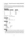
4.9 Example 8
Buoyant jets from a rosette-shaped ocean outfall riser in
natural flow– Hong Kong Strategic Sewage Disposal Scheme (SSDS)
The file is tut8.vj.
In modern ocean outfalls, sewage effluent is often discharged through a number of adequately
spaced outfall risers; the effluent is discharged as a jet group from each of the risers in a `rosette'
like pattern. The planned ocean outfalls for the Hong Kong Strategic Sewage Disposal Scheme
(SSDS), as well as the Shanghai Sewage Project Outfall, are examples of outfalls of this type. The
main parameters for the SSDS outfall with a six-jet group are as follows:
Ambient Parameters:
Depth (m)
0
5.5
11
16.5
22
Salinity (ppt)
25.5
31.2
33.7
34.2
34.5
Current velocity
Temperature (ºC)
27.7
27.8
25.0
23.6
23.0
0.2 m/s (Current Angle=90º)
(N.B. The salinity is expressed in parts per thousand, ppt)
Outfall Parameters:
Depth
Temperature
Salinity
24.0 m
25 ºC
10 ppt
Riser Parameters:
Flow
Distance
T. Radius
B. Radius
Height
0.94164 m³/s
0m
1.5 m
2m
3m
Jet Parameters:
jet 1
jet 2
jet 3
Flow (m³/s)
0.15694
0.15694
Diameter (m)
0.25
Port height (m)
jet 5
jet6
0.15694 0.15694
0.15694
0.15694
0.25
0.25
0.25
0.25
0.25
2
2
2
2
2
2
Vertical angle
0º
0º
0º
0º
0º
0º
Horizontal angle
0º
60º
120º
180º
240º
300º
Salinity (ppt)
10
10
10
10
10
10
Temperature (ºC) 25
25
25
25
25
25
General Notes:
37
jet 4
1. In the Cutting plane window, the user can obtain a Composite dilution for merged
bent-over jets when the Vertical plane (cross-section view) is selected.
2. At the startup window, select Open, open tut8.vj in the folder tutorial files
3. In this case, the measured salinity and temperature at different depths are used as input, linear
variation is assumed between the consecutive adjacent levels. The sum of the six jet discharge
flows is equal to the flow of the riser. All jets discharge horizontally (vertical angle = 0º); only
the horizontal jet discharge angle (relative to the current) is different (0º = coflow; 90º =
perpendicular crossflow; 180º = counterflow).
4. Use the animation function to see the computed rosette jet group pattern, and how different jets
merge with each other. Click the toolbar
to see active process of evolution and spread of
the jet from source to trapped level. Use the Rotate, Zoom, and Move functions to view the jet
cross-section from different angles. Observe how the plumes can merge with each other (even
kinematically). The merging of the multiple plumes is related to the definition of near field
dilution and mixing zone in environmental impact assessment.
5. View the jet from a horizontal plane and in a vertical section. i) Click toolbar
and select
Horizontal plane or Vertical plane with desired distance and input data in Cutting Plane
window. For example, by selecting Vertical plane (cross-section view) and setting distance =
16 m, you will get a cutting vertical plane and this plane is also shown in small window in the
screen---Cross Section. ii) Click any point in Cross Section window, then you can use toolbar
to zoom the plane or use toolbar
to move the plane in Cross Section window.
6. View some characteristics of jet cross-section.
i) Put the cursor on any blue point in Cross Section window, you will get the position of this
point and concentration in Concentration Info window. You will see that the concentration
at a point where adjacent plume elements overlap is larger than that at a non-overlap point,
because of the plume merging.
ii) Click the jet number shown in input parameter window to get the jet cross-sectional area
(area of this Lagrangian element) for the selected jet, the total plume area (with overlapped
area subtracted) and sum of areas of the jets (summation of the projected area of each
individual jet) in this cutting plane. For example, in this case with selecting Vertical plane
(cross-section view) and setting distance = 16 m, the area of jet1, jet2, jet3, jet4, jet5 and
jet6 is 7.9, 32.2, 66.9, 71.5, 66.9 and 32.2m² respectively, the sum of the areas of the six
jets is 277.6 m², and total jet area in the plane is 214.7 m² (excluding overlap). The ratio of
the total jet area to the sum of areas is a measure of reduced dilution due to plume
merging. You can also obtain the composite dilution in the Cutting plane window. (Note:
the computed composite dilution is only valid up to the point where the plume
surfaces or settles to an equilibrium level)
7. Create three identical six-jet risers and observe the merging between adjacent jets, and also
between plumes from adjacent risers, in both uniform flow and under stratified ambient
conditions.
8. Create different orientations of the diffuser axis with respect to the current by changing the
current angle in the ambient parameter window as well as multiple diffusers.
9. Try to explore all the functions on the preceding tutorials 1-7.
38
The following photo shows the observed jet mixing of an 8-jet rosette-jet group in a
laboratory experiment.
Congratulations!
You have successfully finished all the tutorials.
39
5. Advanced graphics features (for experienced users)
5.1 Main components
5.1.1 Toolbar
The toolbar can be moved around the whole screen and provides quick access to various actions
for manipulating the images in the 3D outfall View and the Cross Section View.
Click
To
move
zoom
rotate
cutting plane
pick
solid animation
particle tracing
refresh
5.1.2 Cross section view
The Cross Section (cutting plane projection) View shows the cross sections of the buoyant jets
projected on the cutting plane. The jet sections are coloured. Moving the mouse or pointing device
inside the panel and click, this view will be selected. Moving the mouse with the left button being
pressed down, the cross-section will be zoomed in or out. Moving the mouse with the left button
and the key CTRL being pressed down, you can drag the cross-section into any position in this
view.
40
5.1.3 3D outfall view
This view provides the users with the 3D animation of the jets simulated. Users can obtain different
look of the jets from different angles.
5.1.4 Result data view
This panel displays the information resulted from the simulation. These include: the disk
information, the cross section concentration and area. Information about the cutting plane is
provided.
41
5.2 Graphics manipulation
5.2.1 Actions
5.2.1.1 Zoom
Select
or press the right mouse button and select “Zoom”.
By moving the cursor upward, you can zoom out from the current setting.
By moving the cursor downward, you can zoom in towards the centre of current setting.
5.2.1.2 Move
Select
or press the right mouse button and select “Move”.
Simply using the mouse or pointing device will allow you to move the viewing window to where you
want.
5.2.1.3 Rotate
Select
or press the right mouse button and select “Rotate”.
By moving it in the vertical direction, rotation can be made about the horizontal axis running along
the screen. If the cursor is moved in the horizontal direction, rotation will be made about the vertical
axis running along the screen.
5.2.1.4 Cutting plane
Select
or press the right mouse button and select “Plane”.
Five options are provided when defining a cut plane:
(1) Horizontal plane--- the plane parallel to the surface of the sea.
(2) Front vertical plane--- the plane parallel to the current.
(3) Side vertical plane--- the plane normal to the current.
(4) Normal plane---the cross-section plane normal to the jet trajectory.
(5) User-specified plane---two angles need to be specified by the user. The meanings of the
angles are shown in the cutting plane parameters.
5.2.1.5 Pick
Select
or press the right mouse button and select “Pick”.
Using the cursor, the user can pick or select any point on the jets and display the computed
properties of the disk (including the centre’s position, radius, thickness, orientation, concentration
and velocities) containing that point.
5.2.1.6 Solid animation
Select
The animation of the jet evolution will be re-run.
42
5.2.1.7 Particle tracing
Select
Tracer pattern following the fluid gives a feeling for the velocity at different elevations.
5.2.1.8 Refresh
Select
The evolution process of the jets will be re-run in the 3D Outfall View.
5.2.2 Option
5.2.2.1 Fast display mode
Press the right mouse button and select “Fast Display”.
The fast display mode has less demand upon the graphics capability of the computer and allows a
faster response in changing the displayed graphics. When displaying multiple jets, the normal
display mode has the transparent effect. The user could tell which jet is far from him and which is
near to him. The fast display mode does not have the transparent effect, the user would not see the
jet which is hindered by the front one. Also, with the fast mode, the user could not see the change of
concentration on the jet.
5.2.2.2 Display cutting plane
Press the right mouse button and select “Display Cutplane”.
The cutting plan can be displayed or hidden.
5.2.2.3 Show concentration change
Press the right mouse button and select “Show Concentration Change”.
Display the change in concentration by gradual change in colour.
5.2.2.4 Show velocity change
Press the right mouse button and select “Show Velocity Change”.
Display the change in velocity by gradual change in colour.
5.3 Option menu command
The Option Menu offers the following commands:
Animation speed
Continuous mode
Max number of steps
Disturbance of the
water surface
Water surface
property
Select the animation speed among “fast”, “medium” and “slow”
Require the simulation to continue up to the maximum simulation
step
Allow the user to specify the maximum number of simulation steps
(default no. is 1500)
Show or stop the animated disturbance of the water surface
Allow the user to change the display properties of the water surface
43