1
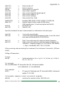
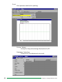
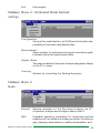
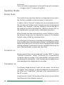
INSTRUCTION
MANUAL
®
MODELS 2635
150 KHz to 1.05 GHz SPECTRUM ANALYZER
Spectrum Analyzer 2635
Technical Characteristics ....................................................... 6
The Interface .................................................................... 7
The Software .................................................................... 7
PR 261 EMI Near Field Sniffer Probe Set (Optional accessories) 10
Specifications .................................................................. 10
General Information ...........................................................
Symbols .........................................................................
Tilt handle .......................................................................
Safety ............................................................................
Operating Conditions ........................................................
Warranty ........................................................................
Maintenance ...................................................................
Selecting the Line Voltage .................................................
Introduction ....................................................................
Operating Instructions ......................................................
11
11
11
12
13
13
14
14
15
16
Control Elements ................................................................ 17
Operation - first steps ......................................................... 27
St. 201000 Zim/tke
Introduction to Spectrum Analysis ....................................... 29
Types of Spectrum Analyzers ............................................ 30
Spectrum Analyzer Requirements ...................................... 32
Frequency Measurements ................................................ 32
Resolution ...................................................................... 33
Sensitivity ...................................................................... 33
Video Filtering ................................................................. 34
Spectrum Analyzer Sensitivity ............................................ 35
Frequency Response ........................................................ 36
Tracking Generators ......................................................... 36
2
CODES for serial Interface RS232 .......................................... 38
Subject to change without notice
Table of contents
Software
AK-2635
Software package AK-2635 .................................................................42
Pulldown Menu 1: ............................................................... 42
Data .............................................................................. 42
Pulldown Menu 2: (Command Mode Normal) ....................... 45
Settings ......................................................................... 45
Pulldown Menu 3: ...............................................................
Operating Modes ............................................................
Normal Mode ..................................................................
Correction on ..................................................................
Calculation on .................................................................
EMC Mode Functions, Software tasks ................................
Definition of new components ...........................................
Configuration of a test system ...........................................
Definition of limit lines ......................................................
Define Test .....................................................................
45
46
46
46
46
47
48
50
51
52
EMC Test Procedure ............................................................ 54
Subject to change without notice
3
NOTES
4
Subject to change without notice
NOTES
Subject to change without notice
5
2635 Spectrum Analyzer for EMC Measurements
Continuous frequency range from 150 kHz to 1050 MHz.
Amplitude range from –100 dBm to +13 dBm
(7 dBµV to 120 dBµV) 80 dB on-screen
Resolution bandwidths of 9 kHz, 120 kHz, 400 kHz
Intermodulation-free dynamic range 75 dB
Save / Recall
Technical Characteristics
The new spectrum analyzer 2635 is
based in general on the
high frequency characteristics of the
2625 and the 2630 analyzers.
The
usable frequency range is therefore from
150 kHz to above 1 GHz. The available
resolution bandwidths are 9kHz, 120kHz
and 400 kHz. Completely new is primarily
the processor-controlled operation and a
digital signal display which works in realtime, and is resolved with up to 4,000
points over the entire screen. The screen
will also display all selected frequency
settings and the marker results.
6
The unique features of this spectrum
analyzer are the extensive EMC measurement capabilities. These include the amplitude indication in Peak and Average
modes. For the precise evaluation of the
signals a marker is provided that will give
a readout for amplitude and frequency
on-screen.
An additional advantage is that newly
acquired signals can be compared with
the content of the reference storage.
Complicated and repeatedly used equipment adjustments can be saved by use of
the Save/Recall function.
Subject to change without notice
2635
The Model 2635 includes a tracking generator that can be used to evaluate the
frequency characteristics of 4-terminal devices, such as filters.
The Interface
The Analyzers are supplied with an RS-232 interface for PC communication and
print-out.
The Software
The software for extended functions and for the evaluation of measurement results
via PC is part of the spectrum analyzer and provides the following features:
Numeric indication of measurement values.
Average, peak and quasi peak values with
corresponding cursor.
Storage of reference spectra for comparison.
Freely definable limit lines.
Indication of above-limit signals.
Correction factors for antennas.
Script-control for automatic measurements.
Printout in tabular form (e. g. table calculations).
B/W or color printouts of the spectra with printer selection for all printers
supported by Windows ©.
On line “Help” function.
A manual for various EMC applications is provided.
Screen Dump of Software AK-2635
Subject to change without notice
7
Specifications
Frequency
Frequency Range:
0.15 MHz to 1050MHz
Frequency Resolution displayed:
10kHz (5½ Digit in Readout)
Center Frequency Range
0.15 MHz - 1050 MHz
Accuracy:
±100kHz
Stability (Drift):
<150kHz/hour
Span:
Zero span and 100kHz/Div to 100MHz/Div
in steps of 1-2-5-10
Accuracy:
±5%
Marker:
absolute Marker
Marker Resolution (Frequency)
5½ digits
Marker Resolution (Level)
3½ digits
Marker Readout Accuracy:
±(0.1%span+100kHz)
Resolution Bandwidth, RBW (3dB):
9kHz, 120kHz and 400kHz
Video Bandwidth, VBW:
4kHz
SWT (fixed):
40ms, 320ms, 1s(1)
Amplitude
Measurement Range:
–100dBmto+13dBm
Displayed Average Noise Level:
–102dBm (120kHz RBW)
Frequency Response
Relative to 500 MHz, ATTN 10 dB
±2dB
Input Attenuator Range:
40 dB, 10 dB steps
Accuracy (reference level):
±1dB
Maximum Safe Input Level
Attenuator setting 20db:
+20dBm(0,1W)
Attenuator setting 0dB:
+10dBm
DC:
±25V
Display Range:
40, 80 dB, 8 Divisions
Scale Units
dBm
Reference Level:
-99to+13dBm(+var.)
Resolution Bandwidth Switching Uncertainty:
±1dB
Spurious responses:
Intermodulation (3rd Order):
–75 dBc
(2 Signals, –27 dBm each, Frequency distance>3MHz)
Harmonic Distortion (2nd, 3rd):
<–75dBc
Absolute Amplitude Accuracy:
±2.5dB
Inputs / Outputs
Front Panel
Input Connector
Probe Power:
Tracking Generator Out (HM5014)
8
BNC (F) Impedance: 50Ω
6V (Near field probes)
BNC (F) Impedance: 50Ω
Subject to change without notice
Special Functions
Average
SAVE/RECALL
Peak-Detection
Max. Hold
Hold
Reference Curve
AM-Demodulator
32 measurements
9 complete Set-ups
Trace stored on screen
Ear Phones
Tracking Generator
Output Frequency Range:
Output Power Level
Output flatness (150 kHz to 1 GHz)
Spurious Outputs
Harmonic Spurs
Non-Harmonic Spurs
150 kHz to 1050 MHz
–50dBmbis+1dBm
±1.0dB
>20dBc
>20dBc
General
Temperature Range
Operating
Storage:
Power Requirements:
Voltage
Frequency
Power consumption
CRT:
Protective System:
Dimensions
Weight:
10°C to40°C
–40°Cto70°C
115/230V
50-60Hz
approx.43VA
8 x 10cm
Safety Class I (IEC 1010-1)
W 285, H 125, D 380mm
approx.: 6kg
1) only if EMC set-up is used
Subject to change without notice
06/98
Accessories supplied
Software for evaluation,
Power Cable, Operating Manual.
Optional accessories
Telescope Antenna
AT-21
HZ520
Near Field Probes (E, H, High Imp. Probe)
PR-261
HZ530
Subject to change without notice
9
HZ530 EMI Near Field Sniffer Probe Set
PR-261
The HZ530
PR-261 is the ideal toolkit for the
investigation of RF electromagnetic fields.
It is indispensible for EMI pre-compliance
testing during product development, prior
to third party testing. The set includes 3
hand-held probes with a built-in preamplifier covering the frequency range from
10 kHz to 1000 MHz depending on probe
type. The set includes one magnetic field
probe, one electric field probe and one
high impedance probe. All have high
sensitivity and are matched to the 50Ω
inputs of spectrum analyzers. The power
can be supplied either from the batteries or
thrugh a power cord directly connected to
2635
an HM5012/14
series spectrum analyzer.
2635
Signal feed is via a 1.5m BNC-cable. When
used in conjunction with a spectrum analyzer
or a measuring receiver, the probes can be
used to locate and qualify EMI sources.
They are especially suited to locate emission
“hot spots” on PCBs and cables, as well as
evaluate EMC problems at the breadboard
and prototype level. They enable the user
to evaluate radiated fields and perform shield
effectivity comparisons. Mechanical
screening performance and immunity tests
on cables and components are easily
performed. Faulty components and poor
bonding locations can be isolated.
The magnetic probe incorporates a high
degree of rejection of both stray and direct
electric fields, and provides far greater
(Optional accessories)
repeatability than with conventional field
probes. Measurements can be made on
the very near field area that is close to
components or radiation sources. The
electric field (mono-pole) probe has the
highest sensitivity of all three probes. It
can be used to check screening and perform pre-compliance testing on a comparative basis. The high impedance probe
is used to measure directly on the components under test or at the conductive
trace of a PC board. It has an input
capacitance of only 2pF and supplies
virtually no electrical charge to the device
under test.
Specifications
Frequency
Frequency range:
0.1MHz to 1000MHz
(lower frequency limit
depends on probe type)
Output impedance:
50 Ω
Output connector:
BNC-jack
Input capacitance:
2pF
(high imped. probe)
Max. Input Level:
+10dBm
(without destruction)
1dB-compression point: -2dBm
(frequency range dependent)
DC-input voltage:
20Vmax.
Supply Voltage:
6VDC
4 AA size batteries
10
2635
Supply-powerofHM5012/5014
Supply Current:
8mA (H-Field Probe)
15mA (E-FieldProbe)
24mA(Highimp.Probe)
Probe Dimensions:
40x19x195mm (WxDxL)
Housing:
Plastic; (electrically
shielded internally)
Package contents:
Carrying case
1 H-Field Probe
1 E-Field Probe
1 High Impedance Probe
1 BNC cable (1.5m)
1 Power Supply Cable
(Batteries or Ni-Cads are not included)
Subject to change without notice
General Information
The HM5012/14
2635 spectrum
analyzer
is easy
operate.
The logical
The
spectrum
analyzer
is to
easy
to operate.The
logical
arrangement of the controls allows anyone to quickly become
familiar with the operation of the instrument, however, experienced
users are also advised to read through these instructions so that
all functions are understood. Immediately after unpacking, the
instrument should be checked for mechanical damage and loose
parts in the interior. If there is transport damage, the supplier must
be informed immediately. The instrument must then not be put
into operation.
Symbols
ATTENTION - refer to manual
Danger - High voltage
Protective ground (earth) terminal
Tilt handle
To view the screen from the best angle, there are three different
positions (C, D, E) for setting up the instrument. If the instrument
is set down on the floor after being carried, the handle
automatically remains in the upright carrying position (A). In order
to place the instrument onto a horizontal surface, the handle
should be turned to the upper side of the Spectrum Analyzer (C).
For the D position (10° inclination), the handle should be turned
to the opposite direction of
the carrying position until
it locks in place automatically underneath the instrument. For the E position
(20° inclination), the handle should be pulled to release it from the D position
and swing backwards until
it locks once more. The
handle may also be set to
a position for horizontal carrying by turning it to the upper side to
lock in the B position. At the same time, the instrument must be
lifted, because otherwise the handle will jump back.
Subject to change without notice
11
Safety
This instrument has been designed and tested in accordance with
IEC Publication 1010-1, Safety requirements for electrical
equipment for measurement, control, and laboratory use. The
CENELEC regulations EN 61010-1 correspond to this standard. It
has left the factory in a safe condition. This instruction manual
contains important information and warnings which have to be
followed by the user to ensure safe operation and to retain the
Spectrum Analyzer in a safe condition. The case, chassis and all
measuring terminals are connected to the protective earth contact
of the appliance inlet. The instrument operates according to Safety
Class I (three-conductor power cord with protective earthing
conductor and a plug with earthing contact). The mains/line plug
shall only be inserted in a socket outlet provided with a protective
earth contact. The protective action must not be negated by the
use of an extension cord without a protective conductor.
The mains/line plug should be inserted before connections are
made to measuring circuits. The grounded accessible metal parts
(case, sockets, jacks) and the mains/line supply contacts (line/
live, neutral) of the instrument have been tested against insulation
breakdown with 2200V DC. Under certain conditions, 50Hz or 60Hz
hum voltages can occur in the measuring circuit due to the interconnection with other mains/line powered equipment or
instruments. This can be avoided by using an isolation transformer
(Safety Class II) between the mains/line outlet and the power plug
of the device being investigated. Most cathode-ray tubes develop
X-rays. However, the dose equivalent rate falls far below the
maximum permissible value of 36pA/kg (0.5mR/h). Whenever
it is likely that protection has been impaired, the instrument shall
be made inoperative and be secured against any unintended
operation. The protection is likely to be impaired if, for example,
the instrument
• shows visible damage,
• fails to perform the intended measurements,
• has been subjected to prolonged storage under unfavourable
conditions (e.g. in the open or in moist environments),
• has been subject to severe transport stress (e.g. in poor
packaging).
12
Subject to change without notice
Operating Conditions
The instrument has been designed for indoor use. The permissible
ambient temperature range during operation is +10°C (+50°F) ...
+40°C (+104°F). It may occasionally be subjected to temperatures
between +10°C (+50°F) and –10°C (+14°F) without degrading its
safety. The permissible ambient temperature range for storage
or transportation is –40°C (+14°F) ... +70°C (+158°F).
The maximum operating altitude is up to 2200m. The maximum
relative humidity is up to 80%.
If condensed water exists in the instrument it should be
acclimatized before switching on. In some cases (e.g. instrument
extremely cold) two hours should be allowed before the
instrument is put into operation. The instrument should be kept
in a clean and dry room and must not be operated in explosive,
corrosive, dusty, or moist environments. The spectrum analyzer
can be operated in any position, but the convection cooling must
not be impaired. For continuous operation the instrument should
be used in the horizontal position, preferably tilted upwards,
resting on the tilt handle.
The specifications stating tolerances are only valid if the
instrument has warmed up for 60 minutes at an ambient
temperature between +15°C (+59°F) and +30°C (+86°F).
Values without tolerances are typical for an average
instrument.
Subject to change without notice
13
Maintenance
Various important properties of the spectrum analyzer should be
carefully checked at certain intervals. Only in this way it is certain
that all signals are displayed with the accuracy on which the
technical data are based.
The exterior of the instrument should be cleaned regularly with a
dusting brush. Dirt which is difficult to remove on the casing and
handle, the plastic and aluminium parts, can be removed with a
moistened cloth (99% water +1% mild detergent). Spirit or washing benzine (petroleum ether) can be used to remove greasy dirt.
The screen may be cleaned with water or washing benzine (but
not with spirit (alcohol) or solvents), it must then be wiped with a
dry clean lint-free cloth. Under no circumstances may the cleaning
fluid get into the instrument. The use of other cleaning agents
can attack the plastic and paint surfaces.
Selecting the Line Voltage
The spectrum analyzer operates at mains/line voltages of 115V
AC and 230V AC. The voltage selection switch is located on the
rear of the instrument and displays the selected voltage. The
correct voltage can be selected using a small screwdriver.
Remove the power cable from the power connector prior to
making any changes to the voltage setting. The fuses must also
be replaced with the appropriate value (see table below) prior to
connecting the power cable. Both fuses are externally accessible
by removing the fuse cover located above the 3-pole power
connector.
14
Subject to change without notice
The fuseholder can be released by pressing its plastic retainers
with the aid of a small screwdriver. The retainers are located on
the right and left side of the holder and must be pressed towards
the center. The fuse(s) can then be replaced and pressed in until
locked on both sides.
Use of patched fuses or short-circuiting of the fuseholder is not
permissible; B&K
HAMEG assumes no liability whatsoever for any
damage caused as a result, and all warranty claims become null
and void.
Fuse type:
Size 5 x 20 mm; 250-Volt AC;
must meet IEC specification 127,
Sheet III (or DIN 41 662 or
DIN 41 571, sheet 3).
Time characteristic: time-lag
Line voltage 115V~ ±10%:
Line voltage 230V~ ±10%:
.
Fuse rating: T 630mA
Fuse rating: T 315mA
Introduction
The spectrum analyzer permits the detection of spectrum
components of electrical signals in the frequency range of 0.15
to 1050MHz. The detected signal and its content have to be
repetitive. In contrast to an oscilloscope operated in Yt mode,
where the amplitude is displayed on the time domain, the
spectrum analyzer displays amplitude on the frequency domain
(Yf). The individual spectrum components of “a signal” become
visible on a spectrum analyzer. The oscilloscope would display
the same signal as one resulting waveform.
The spectrum analyzer works according to the triple superhet
receiver principle. The signal to be measured (fin = 0.15MHz to
1050MHz) is applied to the 1st mixer where it is mixed with the
signal of a variable voltage controlled oscillator (fLO 1350MHz 2350MHz). This oscillator is called the 1st LO (local oscillator). The
difference between the oscillator and the input frequency (fLO fin = 1st IF) is the first intermediate frequency, which passes
through a waveband filter tuned to a center frequency of 1350MHz.
It then enters an amplifier, and this is followed by two additional
mixing stages, oscillators and amplifiers. The second IF is
Subject to change without notice
15
29.875MHz and the third is 2.75MHz. In the third IF stage, the
signal can be selectively transferred through a filter with 400kHz
or 20kHz bandwidth before arriving at an AM demodulator. The
logarithmic output (video signal) is transferred directly, or via a low
pass filter to another amplifier. This amplifier output is connected
to the Y deflection plates of the CRT.
The X deflection is performed with a ramp generator voltage. This
voltage can also be superimposed on a dc voltage which allows
for the control of 1st LO. The spectrum analyzer scans a frequency
range depending on the ramp height. This span is determined by
the scanwidth setting. In ZERO SCAN mode only the direct voltage
controls the 1st LO.
2635 also includes a tracking generator. This generator
The HM5014
provides sine wave voltages within the frequency range of 0.15
to 1050MHz. The tracking generator frequency is determined by
the first oscillator (1st LO) of the spectrum analyzer section.
Spectrum analyzer and tracking generator are frequency
synchronized.
Operating Instructions
It is very important to read the paragraph “Safety” including the
2635
instructions prior to operating the HM5012/14.
No special
2635.
knowledge is necessary for the operation of the HM5012/14.
The
straightforward front panel layout and the limitation to basic
functions guarantee efficient operation immediately. To ensure
optimum operation of the instrument, some basic instructions
need to be followed.
Attention!
2635 is
The most sensitive component of the HM5012/HM5014
is
the input section of the spectrum analyzer. It consists of
the signal attenuator and the first mixer. Without input
attenuation, the voltage at the input must not exceed
+10dBm (0.7Vrms) AC or ±25 volt DC. With a maximum
input attenuation of 40dB the AC voltage must not exceed
+20dBm.
These limits must not be exceeded
otherwise the input attenuator and/or the first mixer would
be destroyed.
16
Subject to change without notice
When measuring via a LISN (line impedance stabilization
network) the input of the Spectrum Analyzer must be
protected by means of a transient limiter.
Prior to examining unidentified signals, the presence of
unacceptable high voltages has to be checked. It is also
recommended to start measurements with the highest possible
attenuation and a maximum frequency range (1000MHz). The user
should also consider the possibility of excessively high signal
amplitudes outside the covered frequency range, although not
displayed (e.g. 1200MHz). The frequency range of 0Hz to 150kHz
is not specified for the HM5012/14
spectrum analyzer. Spectral
2635
lines within this range would be displayed with incorrect amplitude.
A particularly high intensity setting shall be avoided. The way
signals are displayed on the spectrum analyzer typically allows for
any signal to be recognized easily, even with low intensity.
Due to the frequency conversion principle, a spectral line is visible
at 0Hz. It is called IF-feedthrough. The line appears when the 1st
LO frequency passes the IF amplifiers and filters. The level of
this spectral line is different in each instrument. A deviation from
the full screen does not indicate a malfunctioning instrument.
Control Elements
BK Precision
(1) POWER
After about 10 sec. the noise level will appear on the bottom
base line.
Subject to change without notice
17
(2) INTENS: Beam intensity adjustment.
(3) FOCUS: Beam sharpness adjustment.
(4) TR:
Trace Rotation - In spite of Mumetal-shielding of CRT, effects of
earth’s magnetic field on the horizontal trace position cannot be
completely avoided. A potentiometer accessible through an
opening can be used for correction. Slight pincushion distortion
is unavoidable and cannot be corrected.
(5) A/B/A-B:
The instrument has two memories, memory A and memory B.
Actual measurement results are always stored in A, whereby
memory B can only accept copies of memory A results. Function
A-B allows for the subtraction of B results from updated
measuring results stored in A.
Retrieve:
Displays of memory A, B and balance of memory results (A-B)
can be achieved by quickly pushing the A/B, A-B button. The
readout on the screen will inform the user which storage space
is being displayed on screen.
Remark:
After copying A to B, memory of B is displayed. By pushing button
„A/B, A-B“ short it switches to A-B, and another short push to
display A. The readout will show if „A“, „B“ or „A-B“ is currently
displayed.
(6) SAVE:
For storing of up to 10 configuration settings. If a setup was saved,
it can be retrieved via the RECALL button. Frequently used
settings can be reenacted quickly and error-free. The saved
information is retained also when the unit is separated from power
or switched off.
How to choose the SAVE memory location:To choose memory
location quickly push SAVE repeatedly up to number 9 location,
and to return back to 0 location push RECALL button.
Storing:
After selection of memory location push SAVE long to save setting
and to leave SAVE function.
18
Subject to change without notice
BK Precision
Remark:
Functions AVERAGE and MAX.HLD cannot be part of a storage
operation, meaning that SAVE cannot be performed if these
functions are activated. An acoustic signal will alert the user in
this case.
Interrupt:
If no instrument setting is to be saved the SAVE setting will
automatically be deactivated after 3 sec.
(7) RECALL
This function allows to RECALL stored instrument settings from
SAVE.
To activate: Press RECALL long.
Remark:
The RECALL function can not be performed if AVERAGE or
MAX.HOLD are activated. An acoustic signal will alert the user in
this case.
Choose memory location:
To choose memory location quickly push SAVE repeatedly up to
number 9 location, and to return back to 0 location push RECALL
button.
To call-up: After selecting desired memory location, push RECALL
long and instrument will display stored parameter settings.
Subject to change without notice
19
Interrupt: If no instrument setting is to be saved the SAVE setting
will automatically be deactivated after 3 sec.
(8) A B:
Allows for temporary storage of settings from memory A to
memory B for comparison purposes. Push short to store the actual
contents of A in B. The instrument will automatically display stored
B memory. To get back to the actual signal, push „A/B/A-B“ two
times. If pushed one time, „A B“ will be displayed.
Memory contents of B will be deleted when power is turned off.
(9) Max.HLD. (Maximum Hold)
This function allows the automatic storage of maximum signal
level readings of the instrument. The display of the measurement
results will only be updated if the measured value exceeds
previously gathered values. Any smaller as previously recorded
measurements will not be displayed. This function therefore
accurately records maximum signal values of pulsating RF signals.
Therefore, prior to taking measurement readings it should be
made sure that measurement result display has been maximized.
Remark:
Pulsating signals should be recorded in lowest-possible SPAN,
highest-possible Bandwidth and with video filter turned off in order
to prevent transient response errors of the filters. If settings of
span and RBW are set in certain ways, something can be gained
by the slower sweep speed, active in some settings.
Pull-up: Push Max. HLD. The respective LED will light to show
function is activated.
Remark:
To erase display of a measurement (Max.HLD), function Max.HLD
has to be terminated and re-activated to be used again. Switching
to AVERAGE directly will not affect the memory contents of Max.
HLD.
Interrupt: Push Max.HLD. Respective LED will turn off and
indicate interruption of Max.HLD function.
(10) AVERAGE
This function allows the automatic storage of average signal level
readings of the instrument. Using the AVERAGE function the
displayed noise band can be reduced. Thus, signals that would
20
Subject to change without notice
otherwise not be visible due to the noise floor on screen, can be
observed clearly. The AVERAGE function is activated by pushing
the AVERAGE button a short time. The respective LED will light
to show function is activated.
Remark:
The noise reduction (digital) using the AVERAGE function will
not affect amplitude accuracy even for bigger spans, as would
the video filter. So digital averaging doen’t have the response
time limitation that a video filter possesses.
Pull-up: Push AVERAGE. The respective LED will light to show
function is activated.
Remark:
To erase display of a measurement (AVERAGE), function
AVERAGE has to be terminated and re-activated to be used again.
Switching to MAX. HLD. will not affect the memory contents of
AVERAGE.
Interrupt: Push AVERAGE. Respective LED will turn off and
indicate interruption of AVERAGE function.
BK Precision
(11) CENTER FREQ.
By pushing CENTER FREQ. Button, input for center frequency is
being enabled and respective LED is lit. Now Center Frequency
can be adjusted via tuning knob (14). The frequency is displayed
in the upper left-hand corner behind the letter „C“.
Subject to change without notice
21
Remark:
Is center frequency near lower end or SPAN increased, a spectral
line might be visible, possibly even without a signal connected.
It is commonly referred to as „Zero Frequency marking“ (ZERO
Peak) and is not unusual to be seen in analyzers using the superhet
principle. What is observed is the carrier of the 1st LO (1st
Oscillator) to become visible when the frequency comes within
the transmission range of the 1st IF filter. The level of the ZERO
peak mark may be different in each instrument and cannot be
used as calibration level.
(12) FINE
If the FINE button is pushed (LED is lit), frequency inputs (with
LED CENTER FREQ. lit) or Marker movements (LED MARKER is
lit) is performed in very small steps.
Pushing FINE again will cause the more coarse steps to be active
again. The FINE LED will be unlit.
(13) MARKER
In order to evaluate measurement curves, the instrument is
equipped with a running Marker (X). The Marker can be moved in
X-orientation via the tuning dial and follows the measurement
curve in Y-orientation. To activate the Marker, the Marker has to
be activated (LED lit) by pushing MARKER. The numeric indication
of marker frequency and amplitude is displayed on-screen (i.e.:
M 100.00MHz –29dBm). Push CENTER to leave MARKER mode
Remark:
The FINE function also affects the input for the Marker position.
(14) Tuning Dial:
The tuning dial either selects Center Frequency or Marker position,
depending on CENTER FREQ. or MARKER being activated.
(15) SPAN
The span of sweep of the analyzer is set via the two SPAN buttons.
The SPAN is displayed in the upper right-hand corner of the screen
and is marked with the letter „S“. At full SPAN (1000MHz) the
frequency axis is scaled in 100MHz steps per (vertical) graticule
line. Moving from the center graticule line towards the right screen
edge, the frequency increases by 100MHz per each line.
Therefore, the frequency of a displayed spectral line would be
500MHz + 5x100MHz = 1000MHz. The frequency reduces
22
Subject to change without notice
accordingly when moving towards the left screen edge. The
outermost left line therefore corresponds to 0MHz.
(16) ZERO SPAN:
With the ZERO SPAN button a SPAN of 0 Hz is being selected. If
a SPAN of 0Hz is selected, the analyzer performs as a selective
level meter, which can be calibrated via the Center Frequency
(CENTER FREQ.). The display of the measured level is displayed
via a horizontal line. The ZERO SPAN mode is activated by pushing
the ZERO SPAN button. Press again to revert to previous span.
Above illustration explains the terms SPAN, Center Frequency,
Extent of Scale, and Attenuator.
The height
of the „window“ is limited to 80dB due to the extent of the scale,
however, the display range can be shifted up and down by
switching on or off the attenuators and by setting another
reference level. The width of the displayed range is set via the
SPAN of the analyzer, which may comprise of the entire gray
area or only part of it. The location of this range is set via the
Center Frequency (CENTER FREQ.). It is always advisable to
select the precise Center Frequency and the SPAN as low as
possible (resolution of display) so the signal can be viewed easily.
An unnecessarily high SPAN has a rather negative effect.
Remark:
2635
The HM5012/5014
spectrum analyzer is internally programmed
for always choosing the appropriate sweep time related to the
span, resolution bandwidth and video bandwidth, wherever
possible. The UNCAL indicator in the readout will be visible in
Subject to change without notice
23
order to prevent possible measuring errors due to insufficient
transient response time.
(17) 5dB/Div.
Py pushing the 5 dB/Div. button, the vertical scale is set to 5 dB/
Div. The respective LED will then be lit. To enter again in 10 dB/
Div. mode, push 5 dB/Div. again.
(18) RBW (Resolution Bandwidth):
The instrument is equipped with resolution filters of 9kHz, 120kHz,
and 400kHz, which can be selected via the „RBW“ buttons. The
respective LED will indicate which bandwidth is selected.
Remark:
A maximum measuring bandwidth and the Max.HLD function
should be selected for pulsed signals.
BK Precision
(19) VBW-Video Filter:
The Video Filter has the purpose of reducing video and noise
bandwidth and therefore reducing noise distribution. When
measuring low level values, which are situated within the regular
noise level, the Video Filter (low pass) can be used to reduce the
noise level. This allows for the detection of even small signals
which might otherwise not be visible.
Remarks:
Please note that if frequency range (SPAN) is too high and Video
Filter is active, amplitude readings might be wrong (too small)
24
Subject to change without notice
(UNCAL display). In this case, SPAN needs to be reduced. With
the aid of the Center Frequency (CENTER FREQ.) setting, first
the signal to be tested needs to be centered on screen, then the
SPAN can be reduced.
If SPAN is reduced without the signal to be tested centered it is
possible for the signal to end up outside of the screen.
The Video Filter should not be used - if possible - when pulsed
signals are measured in order to prevent measuring errors
(transient response time).
(20) ATTN:
The buttons to set the input attenuation are marked ATTN. By
pushing the UP and DOWN buttons, the attenuation can be set
from 0 dB to 40 dB in 10 dB steps.
To enter 0 dB attenuation, it is neccessary to push button long,
this is for protection of the input stage, so this setting can’t be
set accidentally.
Remark:
For reasons of protection of the input stage, the instrument will
always set an attenuation of 10 dB when switched on.
It needs to be pointed out again that the maximum allowable
input voltages may not be surpassed. This is especially important,
as it may be possible that the spectrum analyzer will display only
part of a signal under test, if other input signals are present but
not visible at current span.
(21) REFERENCE
With rotary knob REFERENCE the so called reference level is
set, to this level all amplitude readings on screen are referenced.
The reference level is always at the topmost horizontal graticule
line. Depending also on attenuator setting, the reference level
may be set between –99.8 dBm and +13 dBm.
(22) INPUT:
50 Ω Input of Spectrum Analyzer. Without attenuation of input
signal the maximum allowable input voltage is ±25V DC or
+10dBm AC respectively. With a maximum attenuation of the
input signal (40dB) +20dBm is allowed. These values may not
be exceeded, otherwise the input stages will be damaged.
Subject to change without notice
25
BK Precision
(23) PROBE POWER:
PROBE POWER is used solely to supply power for the near field
probes PR-261.
HZ530. The required special power cable is supplied with
the probe set.
(24) VOL.: To regulate the volume for the head set.
(25) PHONE:
Connector for headset. The head set should be equipped with a
3.5mm stereo phone connector and have >8 Ohm of impedance.
(26) ATTN.
The TG output attenuator has 5 positions,which can be
chosen via the UP/DOWN-buttons. The output attenuator is used
for reducing the output level of the Tracking Generator.
(27) LEVEL
With the LEVEL knob the output level of the Tracking generator
can be varied in steps of 0.2 dB. The range for level settings is 11
dB. The output level is shown in the readout, also dependent on
the attenuator setting.
Attention:
If Tracking Generator is not activated, the output level can
be still varied, this is visible in the readout. For having
this signal appliued to the output, the Tracking generator
must be activated. This is a security measure to prevent
damages to sensitive loads.
26
Subject to change without notice
BK Precision
(28) Tracking Generator
After switching on the instrument, the Tracking generator will be
inactive. This is a security measure to protect any loads connected.
In the readout this is shown by the minuscule „t“. By pushing
TRACK. GEN., the Tracking Generator is activated. Now a capital
„T“ will appear in the readout, and one of the attenuator LEDs
(26) will be lit. By again pushing TRACK. GEN., the Tracking Generator is deactivated.
(29) Output
50 Ω output of Tracking Generators. The output level is set using
the rotary knob LEVEL (27) and the attenuator buttons (26). The
output level can be set between +1 dBm and –50 dBm.
(30) RM (Remote) LED
The RM-LED indicates that the instrument is controlled via the
serial interface. If the LED is lit, it is not possible to use controls
on front panel. This state can either be ended via a serial
commando, or by switching off the instrument. The remote-mode
can be activated only by a serial command via the interface.
Operation - first steps
Settings:
Before an unknown signal is applied to the input of the instrument,
it should be verified that the DC component is smaller than +-25V
and maximum amplitude is below +20 dBm.
Subject to change without notice
27
ATTN. :
As a protective measure the attenuation should be set to 40 dB
(LED „40“ is lit).
Frequency setting:
Set CENTER FREQ. to 500 MHz (C500MHz) and choose a span
of 1000 MHz.
Bandwidth:
For the first measurements the 400 MHz filter should be selected,
and video filter off.
If the noise band moves upward on screen when decreasing input
attenuation, this indicates a possible other high-amplitude input
signal present but not visible in the chosen frequency range. If no
signal is visible, the attenuation can be consecutively decreased.
In any case the attenuator setting must be in correspondence to
the biggest input signal (not Zero-peak). The correct signal level is
achieved if the biggest signal („0 Hz“ - 1000 MHz) just touches
the reference line. If the signal surpasses the reference line, the
attenuation must be increased, or an external attenuator of suitable
power rating and attenuation must be used.
Measuring in full-span mode serves mostly as a quick overview.
To analyze the detected signals more closely, the span has to be
decreased. Previous to this, the center frequency has to be set so
the signal is at center of screen. Then span can be reduced.
Then the resolution bandwidth can be decreased, and the video
filter used if neccessary. The warning „uncal“ in the readout must
not be displayed, otherwise measurement results may be incorrect.
28
Subject to change without notice
Obtaining values:
For a numerical value of a measurement result the easiest way is
the use of the marker. The marker frequency is set by the rotary
dial, if necessary, use the fine step mode. Then, read the value for
the amplitude, which is shown in the readout. The amplitude is
automatically corrected for the attenuator setting.
If a value is to be measured without using the marker, then
measure the difference of the reference line to the signal. Observe
that the scale may be either 5 dB/Div. or 10 dB/Div. In the reference
level value the setting of the input attenuator is already included,
it is not neccessary to make a correction afterwards.
The signal shown in the picture shows an amplitude difference of
about –16 dB to the reference line. Assuming that the reference
level is –27 dBm, and the scale 10 dB/Div.
Thus the signal has an amplitude of (–27 dBm) + (–16 dB) =
-43dBm. In this value the setting of the input attenuator is already
included. It is not necessary for the user to correct the value for
any attenuator setting.
Introduction to Spectrum Analysis
The analysis of electrical signals is a fundamental problem for
many engineers and scientists. Even if the immediate problem
is not electrical, the basic parameters of interest are often changed
into electrical signals by means of transducers. The rewards for
transforming physical parameters to electrical signals are great,
as many instruments are available for the analysis of electrical
signals in the time and frequency domains.
The traditional way of observing electrical signals is to view them
in the time domain using an oscilloscope. The time domain is
used to recover relative timing and phase information which is
needed to characterize electric circuit behavior. However, not all
circuits can be uniquely characterized from just time domain
information. Circuit elements such as amplifiers, oscillators,
mixers, modulators, detectors and filters are best characterized
by their frequency response information. This frequency
information is best obtained by viewing electrical signals in the
frequency domain. To display the frequency domain requires a
device that can discriminate between frequencies while
measuring the power level at each. One instrument which
displays the frequency domain is the spectrum analyzer. It
Subject to change without notice
29
graphically displays voltage or power as a function of frequency
on a CRT (cathode ray tube).
In the time domain, all frequency components of a signal are
seen summed together. In the frequency domain, complex signals
(i.e. signals composed of more than one frequency) are separated
into their frequency components, and the power level at each
frequency is displayed. The frequency domain is a graphical
representation of signal amplitude as a function of frequency.
The frequency domain contains information not found in the time
domain and therefore, the spectrum analyzer has certain
advantages compared with an oscilloscope.
The analyzer is more sensitive to low level distortion than a scope.
Sine waves may look good in the time domain, but in the
frequency domain, harmonic distortion can be seen. The
sensitivity and wide dynamic range of the spectrum analyzer is
useful for measuring low-level modulation. It can be used to
measure AM, FM and pulsed RF. The analyzer can be used to
measure carrier frequency, modulation frequency, modulation level,
and modulation distortion. Frequency conversion devices can be
easily characterized. Such parameters as conversion loss, isolation,
and distortion are readily determined from the display.
The spectrum analyzer can be used to measure long and short
term stability. Parameters such as noise sidebands on an oscillator,
residual FM of a source and frequency drift during warm-up can
be measured using the spectrum analyzer’s calibrated scans. The
swept frequency responses of a filter or amplifier are examples of
swept frequency measurements possible with a spectrum analyzer.
These measurements are simplified by using a tracking generator.
Types of Spectrum Analyzers
There are two basic types of spectrum analyzers, swept-tuned
and real-time analyzers. The swept-tuned analyzers are tuned by
electrically sweeping them over their frequency range. Therefore,
the frequency components of a spectrum are sampled sequentially
in time. This enables periodic and random signals to be displayed,
but makes it impossible to display transient responses. Real-time
analyzers, on the other hand, simultaneously display the amplitude
of all signals in the frequency range of the analyzer; hence the
name real-time. This preserves the time dependency between
signals which permits phase information to be displayed. Realtime analyzers are capable of displaying transient responses as
well as periodic and random signals.
30
Subject to change without notice
The swept-tuned analyzers are usually of the trf (tuned radio
frequency) or superheterodyne type. A trf analyzer consists of a
bandpass filter whose center frequency is tunable over a desired
frequency range, a detector to produce vertical deflection on a
CRT, and a horizontal scan generator used to synchronize the tuned
frequency to the CRT horizontal deflection. It is a simple,
inexpensive analyzer with wide frequency coverage, but lacks
resolution and sensitivity. Because trf analyzers have a swept filter
they are limited in sweep width depending on the frequency range
(usually one decade or less). The resolution is determined by the
filter bandwidth, and since tunable filters dont usually have constant
bandwith, is dependent on frequency.
The most common type of spectrum analyzer differs from the trf
spectrum analyzers in that the spectrum is swept through a fixed
bandpass filter instead of sweeping the filter through the spectrum.
The analyzer is basically a narrowband receiver which is
electronically tuned in frequency by applying a saw-tooth voltage
to the frequency control element of a voltage tuned local oscillator.
This same saw-tooth voltage is simultaneously applied to the
horizontal deflection plates of the CRT. The output from the
receiver is synchronously applied to the vertical deflection plates
of the CRT and a plot of amplitude versus frequency is displayed.
The analyzer is tuned through its frequency range by varying the
voltage on the LO (local oscillator). The LO frequency is mixed
with the input signal to produce an IF (intermediate frequency)
which can be detected and displayed. When the frequency
difference between the input signal and the LO frequency is equal
to the IF frequency, then there is a response on the analyzer. The
advantages of the superheterodyne technique are considerable.
It obtains high sensitivity through the use of IF amplifiers, and
many decades in frequency can be tuned.
Also, the resolution can be varied by changing the bandwidth of
the IF filters. However, the superheterodyne analyzer is not realtime and sweep rates must be consistent with the IF filter time
constant. A peak at the left edge of the CRT is sometimes called
the “zero frequency indicator” or “local oscillator feedthrough”.
It occurs when the analyzer is tuned to zero frequency, and the
local oscillator passes directly through IF creating a peak on the
CRT even when no input signal is present. (For zero frequency
tuning, FLO=FIF). This effectively limits the lower tuning limit.
Subject to change without notice
31
Spectrum Analyzer Requirements
To accurately display the frequency and amplitude of a signal on
a spectrum analyzer, the analyzer itself must be properly
calibrated. A spectrum analyzer properly designed for accurate
frequency and amplitude measurements has to satisfy many
requirements:
1. Wide tuning range
2. Wide frequency display range
3. Stability
4. Resolution
5. Flat frequency response
6. High sensitivity
7. Low internal distortion
Frequency Measurements
The frequency scale can be scanned in three different modes
full, per division, and zero scan. The full scan mode is used to
locate signals because the widest frequency ranges are displayed
in this mode. (Not all spectrum analyzers offer this mode).
The per division mode is used to zoom-in on a particular signal.
In per division, the center frequency of the display is set by the
Tuning control and the scale factor is set by the Frequency Span
or Scan Width control. In the zero scan mode, the analyzer acts
as a fixed-tuned receiver with selectable bandwidths.
Absolute frequency measurements are usually made from the
spectrum analyzer tuning dial. Relative frequency measurements
require a linear frequency scan. By measuring the relative
separation of two signals on the display, the frequency difference
can be determined.
It is important that the spectrum analyzer be more stable than
the signals being measured. The stability of the analyzer depends
on the frequency stability of its local oscillators. Stability is usually
characterized as either short term or long term. Residual FM is a
measure of the short term stability which is usually specified in
Hz peak-to-peak. Short term stability is also characterized by noise
sidebands which are a measure of the analyzers spectral purity.
Noise sidebands are specified in terms of dB down and Hz away
from a carrier in a specific bandwidth. Long term stability is
characterized by the frequency drift of the analyzers LOs.
Frequency drift is a measure of how much the frequency changes
during a specified time (i.e., Hz/min. or Hz/hr).
32
Subject to change without notice
Resolution
Before the frequency of a signal can be measured on a spectrum
analyzer it must first be resolved. Resolving a signal means
distinguishing it from its nearest neighbours. The resolution of a
spectrum analyzer is determined by its IF bandwidth. The IF
bandwidth is usually the 3dB bandwidth of the IF filter. The ratio
of the 60dB bandwidth (in Hz) to the 3dB bandwidth (in Hz) is
known as the shape factor of the filter. The smaller the shape
factor, the greater is the analyzer’s capability to resolve closely
spaced signals of unequal amplitude. If the shape factor of a filter
is 15:1, then two signals whose amplitudes differ by 60dB must
differ in frequency by 7.5 times the IF bandwidth before they can
be distinguished separately. Otherwise, they will appear as one
signal on the spectrum analyzer display.
The ability of a spectrum analyzer to resolve closely spaced signals
of unequal amplitude is not a function of the IF filter shape factor
only. Noise sidebands can also reduce the resolution. They appear
above the skirt of the IF filter and reduce the offband rejection of
the filter. This limits the resolution when measuring signals of
unequal amplitude.
The resolution of the spectrum analyzer is limited by its narrowest
IF bandwidth. For example, if the narrowest bandwidth is 10kHz
then the nearest any two signals can be and still be resolved is
10kHz. This is because the analyzer traces out its own IF bandpass shape as it sweeps through a CW signal. Since the resolution
of the analyzer is limited by bandwidth, it seems that by reducing
the IF bandwdith infinitely, infinite resolution will be achieved.
The fallacy here is that the usable IF bandwidth is limited by the
stability (residual FM) of the analyzer. If the internal frequency
deviation of the analyzer is 10kHz, then the narrowest bandwidth
that can be used to distinguish a single input signal is 10kHz.
Any narrower IF-filter will result in more than one response or an
intermittent response for a single input frequency. A practical
limitation exists on the IF bandwidth as well, since narrow filters
have long time constants and would require excessive scan time.
Sensitivity
Sensitivity is a measure of the analyzer’s ability to detect small
signals. The maximum sensitivity of an analyzer is limited by its
internally generated noise. This noise is basically of two types:
thermal (or Johnson) and nonthermal noise. Thermal noise power
can be expressed as:
Subject to change without notice
33
PN =k×T×B
where:
PN = Noise power in watts
k = Boltzmanns Constant
(1.38 ⋅ 10-23 Joule/K)
T = absolute temperature, K
B = bandwidth of system in Hertz
As seen from this equation, the noise level is directly proportional to bandwidth. Therefore, a decade decrease in bandwidth
results in a 10dB decrease in noise level and consequently 10dB
better sensitivity. Nonthermal noise accounts for all noise
produced within the analyzer that is not temperature dependent.
Spurious emissions due to nonlinearities of active elements,
impedance mismatch, etc. are sources of nonthermal noise. A
figure of merit, or noise figure, is usually assigned to this nonthermal noise which when added to the thermal noise gives the
total noise of the analyzer system. This system noise which is
measured on the CRT, determines the maximum sensitivity of
the spectrum analyzer. Because noise level changes with
bandwith it is important, when comparing the sensitivity of two
analyzers, to compare sensitivity specifications for equal
bandwidths. A spectrum analyzer sweeps over a wide frequency
range, but is really a narrow band instrument. All of the signals
that appear in the frequency range of the analyzer are converted
to a single IF frequency which must pass through an IF filter; the
detector sees only this noise at any time. Therefore, the noise
displayed on the analyzer is only that which is contained in the IF
passband. When measuring discrete signals, maximum
sensitivity is obtained by using the narrowest IF bandwidth.
Video Filtering
Measuring small signals can be difficult when they are
approximately the same amplitude as the average internal noise
level of the analyzer. To facilitate the measurement, it is best to
use video filtering. A video filter is a post-detection low pass
filter which averages the internal noise of the analyzer. When
the noise is averaged, the input signal may be seen. If the
resolution bandwidth is very narrow for the span, the video filter
should not be selected, as this will not allow the amplitude of
the analyzed signals to reach full amplitude due to its video
bandwidth limiting property.
34
Subject to change without notice
Spectrum Analyzer Sensitivity
Specifying sensitivity on a spectrum analyzer is somewhat arbitrary.
One way of specifying sensitivity is to define it as the signal level
when signal power = average noise power.
The analyzer always measures signal plus noise. Therefore, when
the input signal is equal to the internal noise level, the signal will
appear 3dB above the noise. When the signal power is added to
the average noise power, the power level on the CRT is doubled
(increased by 3dB) because the signal power=average noise power.
The maximum input level to the spectrum analyzer is the damage
level or burn-out level of the input circuit.
+10dBm for the input mixer and +20dBm for the input
attenuator. Before reaching the damage level of the analyzer, the
analyzer will begin to gain compress the input signal. This gain
compression is not considered serious until it reaches 1dB. The
maximum input signal level which will always result in less than
1dB gain compression is called the linear input level. Above 1dB
gain compression the analyzer is considered to be operating
nonlinearly because the signal amplitude displayed on the CRT is
not an accurate measure of the input signal level.
Whenever a signal is applied to the input of the analyzer, distortions
are produced within the analyzer itself. Most of these are caused
by the non-linear behavior of the input mixer.
These
5014 t distortions are typically 70dB below the input signal
level for signal levels not exceeding –27dBm at the input of the
first mixer. To accommodate larger input signal levels, an
attenuator is placed in the input circuit before the first mixer. The
largest input signal that can be applied, at each setting of the
input attenuator, while maintaining the internally generated
distortions below a certain level, is called the optimum input level
of the analyzer. The signal is attenuated before the first mixer
because the input to the mixer must not exeed –27dBm, or the
analyzer distortion products may exceed the specified 70dB range.
This 70dB distortion-free range is called the spurious-free dynamic
range of the analyzer. The display dynamic range is defined as
the ratio of the largest signal to the smallest signal that can be
displayed simultaneously with no analyzer distortions present.
Dynamic range requires several things then. The display range
must be adequate, no spurious or unidentified response can occur,
and the sensitivity must be sufficient to eliminate noise from the
displayed amplitude range.
Subject to change without notice
35
The maximum dynamic range for a spectrum analyzer can be easily
determined from its specifications. First check the distortion spec.
For example, this might be “all spurious products 70dB down for –
27dBm at the input mixer”. Then, determine that adequate
sensitivity exists. For example, 70dB down from –27dBm is –97dB.
This is the level we must be able to detect, and the bandwidth
required for this sensitivity must not be too narrow or it will be
useless. Last, the display range must be adequate.
Notice that the spurious-free measurement range can be extended
by reducing the level at the input mixer. The only limitation, then, is
sensitivity. To ensure a maximum dynamic range on the CRT display,
check to see that the following requirements are satisfied.
1.The largest input signal does not exceed the optimum input level
of the analyzer (typically –27dBm with 0dB input attenuation).
2.The peak of the largest input signal rests at the top of the CRT
display (reference level).
Frequency Response
The frequency response of an analyzer is the amplitude linearity of
the analyzer over its frequency range. If a spectrum analyzer is to
display equal amplitudes for input signals of equal amplitude, independent of frequency, then the conversion (power) loss of the input
mixer must not depend on frequency. If the voltage from the LO is
too large compared to the input signal voltage then the conversion
loss of the input mixer is frequency dependent and the frequency
response of the system is nonlinear. For accurate amplitude
measurements, a spectrum analyzer should be as flat as possible
over its frequency range. Flatness is usually the limiting factor in
amplitude accuracy since it is extremely difficult to calibrate out.
And, since the primary function of the spectrum analyzer is to
compare signal levels at different frequencies, a lack of flatness
can seriously limit its usefulness.
Tracking Generators
The tracking generator is a special signal source
whose RF output frequency tracks (follows) some other signal
beyond the tracking generator itself. In conjunction with the
spectrum analyzer, the tracking generator produces a signal whose
frequency precisely tracks the spectrum analyzer tuning. The
tracking generator frequency precisely tracks the spectrum analyzer
36
Subject to change without notice
tuning since both are effectively tuned by the same VTO. This
precision tracking exists in all analyzer scan modes. Thus, in full
scan, the tracking generator output is a start-stop sweep, in zero
scan the output is simply a CW signal.
The tracking generator signal is generated by synthesizing and
mixing two oscillators. One oscillator is part of the tracking
generator itself, the other oscillator is the spectrum analyzer’s
1st LO. The spectrum analyzer/tracking generator system is used
in two configurations: open-loop and closed-loop. In the openloop configuration, unknown external signals are connected to
the spectrum analyzer input and the tracking generator output is
connected to a counter. This configuration is used for making
selective and sensitive precise measurement of frequency, by
tuning to the signal and switching to zero scan.
In the closed-loop configuration, the tracking generator signal is
fed into the device under test and the output of the device under
test is connected to the analyzer input.
In this configuration, the spectrum analyzer/tracking generator
becomes a self-contained, complete (source, detector, and
display) swept frequency measurement system. An internal
leveling loop in the tracking generator ensures a leveled output
over the entire frequency range. The specific swept measurements that can be made with this system are frequency response
(amplitude vs. frequency), magnitude only reflection coefficient,
and return loss. From return loss or reflection coefficient, the
SWR can be calculated. Swept phase and group delay
measurements cannot be made with this system; however, it
does make some unique contributions not made by other swept
systems, such as a sweeper/network analyzer, a sweeper/
spectrum analyzer, or a sweeper/detector oscilloscope.
Precision tracking means at every instant of time the generator
fundamental frequency is in the center of the analyzer passband,
and all generator harmonics, whether they are generated in the
analyzer or are produced in the tracking generator itself, are outside
the analyzer passband. Thus only the tracking generator fundamental frequency is displayed on the analyzer’s CRT. Second and
third order harmonics and intermodulation products are clearly
out of the analyzer tuning and, therefore, they are not seen. Thus,
while these distortion products may exist in the measurement
set-up, they are completely eliminated from the CRT display.
Subject to change without notice
37
Appendix A
The 1dB gain compression level is a point of convenience, but it
is nonetheless considered the upper limit of the dynamic range.
The lower limit, on the other hand, is dictated by the analyzer
sensitivity which, as we know, is bandwidth dependent. The
narrowest usable bandwidth in turn is limited by the tracking
generator residual FM and any tracking drift between the analyzer
tuning and the tracking generator signal.
CODES for serial interface RS232
Spectrum Analyzer 2635
RS232 parameters when unit is turned on:
4800 baud, 8 data bits, 1 stopbit, no parity
Commands to 2635
5014 via PC:
To be noted: First symbol of any command is „#“ (0x23) which is followed by the
respective characters, i.e. TG for Tracking Generator, and further followed by additional symbols, which are explained in detail below. Each command is executed by pushing
the „Enter“ key (hex: OxOd). No differentiation is made between capital and lowercase letters (i.e. TG = tg). Units of measurement are always definite (i.e. span value
given in MHz) and are therefore not indicated.
(E) = „enter“ key
#kl0 (E)
#kl1 (E)
#tg0 (E)
#TG1 (E)
#vf0 (E)
#Vf1 (E)
#Tl+01.0 (E)
#tl-50.0 (E)
#rl-27.0 (E)
#rl-99.6 (E)
#at0 (E)
#bw400 (E)
#sp1000 E)
#sp0 (E)
#db5 (E)
#db10 (E)
#cf0500.00(E)
38
=
=
=
=
=
=
=
=
=
=
=
=
=
=
=
=
=
Key-Lock off
Key-Lock on (Remote-LED lit)
Tracking Generator off
Tracking Generator on
Video Filter off
Video Filter on
Tracking Level of +1.0 dB
Tracking Level to -50.0 dB in 0.2 dB steps
Reference Level of -27.0 dB
Reference Level to -99.6 dB in 0.4 dB steps
Attenuator 0 (10, 20, 30, 40) dB
Bandwidth 400 (120, 9) kHz
Span 1000 (500, 200, . . . 5, 2, 1) MHz
Zero Span
5 dB/div.
10 dB/div.
Center Frequency in xxx.xx MHz
Subject to change without notice
Appendix A
#dm0 (E)
#dm1 (E)
#sa (E)
#vm0 (E)
#vm1 (E)
#vm2 (E)
#vm3 (E)
#vm4 (E)
=
=
=
=
=
=
=
=
Detect mode off
Detect mode on
Save signal A as signal B
View mode: Signal A
View mode: Signal B (stored signal)
View mode: Signal A - B
View mode: Average
View mode: Max. Hold
#br4800 (E)
#bm1 (E)
=
=
#rc0 (E)
#sv0 (E)
=
=
baudrate 4800 (9600, 19200, 38400, 115200 ) Bd
transfer signal in block mode (2048 bytes)
2044 signal bytes, 3 checksum bytes and (0x0D)
Recall (0 to 9)
Save (0 to 9)
Special commands for emc measurement in combination with zero-span:
#es0 (E)
#es1 (E)
=
=
1 second sweep disable
1 second sweep enable (measuring time 1 second; select
zero-span and bandwidth 9/120/400 kHz)
#ss1 (E)
#ss2 (E)
=
=
Start 1 second sweep at a selected center frequency
Start 1 second sweep at a selected center frequency (i.e
100MHz) + frequency step(s) (i.e. 100.12MHz, 100.24MHz,
...). step = bandwidth: 400, 120, 10 (9) kHz
After receiving and processing the command, the instrument transmitts „RD(hex:
0x0d)“.
Polling of Parameters:
Syntax:
#xx (E)
=
Send parameter xx (xx = tg, tl, rl, vf, at, bw, sp, cf, db, kl,
hm, vn, vm, uc)
1st example:
#uc (uncalibrated): PC transmitts #uc (E), instrument replies:
uc0 (calibrated), uc1 (uncalibrated)
2nd example:
#tl (E)
=
PC query for Tracking Level: PC transmitts #tl(E), instrument
replies: TL-12.4(E)
3rd example: sequence control via external computer:
#kl1 (E)
=
switches to remotes status, RM LED is lit
Subject to change without notice
39
#cf0752.00(E)
#sp2 (E)
#bw120 (E)
#kl0 (E)
=
=
=
=
sets Center Frequency to 752 MHz
sets Span to 2 MHz
sets RBW to 120 kHz
switches back to keyboard mode
4th example:
#vn
=
PC query for software version, i.e. „1.00“.
5th example:
#hm
=
PC query for instrument type, i.e. (5012 or 5014)
40
Subject to change without notice
AK-2635 Computer Software Manual
Manual
Software
SW5012
Subject to change without notice
41
Software package AK-2635
Functions and set-up.
Menu overview.
Pulldown Menu 1:
Data
Load
Save
Settings
Measurement
Load and Save set-up information for the
instrument
Load and Save measurement data
New/Copy
42
Subject to change without notice
Edit
Delete
New, Copy, Edit, Delete regarding to the following items:
Limit Definition
Definition of limit lines
Loss/Gain Components
Set-up of the correction curves for amplifiers, cables etc., acquired
by measured data (damping curve).
Config
Set-up for used equipment and DUT, attachment of correction
curves of amplifiers and cables for calculation purposes.
EMC Test
Test procedure set-up (single test): start frequency, stop
frequency, correction curve, filter settings, etc.
Subject to change without notice
43
Print
Print preview and start of printing.
Printer Setup
Set-up for the printer being attached to the PC
Database Selection
Selection of the database to be used.
44
Subject to change without notice
Exit
Exit program.
Pulldown Menu 2: (Command Mode Normal)
Settings
Configuration
Set-up of the serial interface, set COM port and transfer rate;
possibility of automatic rate identification.
Measurement
Opens window for instrument set-up and a waveform graph
to display the actual measurement data.
Display Mode
Two areas are defined: Spectrum Analyzer and graphic display
on the PC’s screen.
Tracking
Window for controlling the Tracking Generator.
Pulldown Menu 3:
Mode
Normal
Remote operation of the Spectrum Analyzer via PC.
Acquisition, analysis and storage of data on the PC.
EMC
Extended operating procedures for measuring emitted
radiation with an antenna including correction for antenna
gain, damping characteristics of cables and amplifiers, etc.).
Subject to change without notice
45
Autostore
Timer controlled measurement in Normal Mode with automatic
storage in the PC’s memory/hard disk.
Operating Modes:
Normal Mode
This mode of man-machine-interface corresponds one-to-one to
the functions available on the instrument’s front panel.
A mouse click on “Normal” enables the user to remotely control
the functions of the Spectrum Analyzer from the measurement
window. The “Remote” indicator (visible in the second bar of
the window) has to be activated first ( RM) by a mouse click on
the related button (a small hook is visible after activation).
When Remote has been activated any center frequency within
the allowed range may be selected by typing in the desired
numeric value, closed by a carriage return.
The indication for RevLevel is actualized automatically according
to any modification in the attenuator settings. A dedicated window
allows the selection of the unit in which the signal level values
shall be indicated. Furthermore one can configure the set-up for
span, filter bandwidth, scaling, and video filter.
Correction on
Single spectral lines can be analyzed in mode “EMC” in menu
“Function Correction”. When “Correction on” is activated all
correction data according to the selected EMC settings will be
used during the calculations. Limit line data can be loaded at any
time and graphically displayed in the window.
Calculation on
The Display Mode window is split into two areas: the left one
(“Analyzer” and “Settings”) is directly related to the instrument,
the other one (“Read/View”) belongs to the representation on
the PC’s screen.
Using function Save A B the data of the actual curve A will be
transferred into the reference memory.
46
Subject to change without notice
In the “Settings” window ten different instrument set-ups can
be saved and recalled. This responds directly to the front panel
function of the instrument.
There are three different modes to display data after acquisition
by the Spectrum Analyzer: “Sample” (actual curve A),
“Reference B” or “A-B”. When the function “Calculation” is
activated one of the following curves may be indicated: “Max.
Hold” or “Average”. The “Max. Hold” and “Average” curves
are calculated in real-time. After a mouse click on button “Reset
Calculation” the sampling will be started anew. The window in
the right area (“Read/View”) enables the user to select the data
type to be transferred from the instrument to the PC and the
curve(s) to be displayed on the screen. The attached colors are
explained at the right edge of the window, the time stamp for
the last acquisition is indicated at the upper edge. The calculation
of the curve data is switched off with “Calculation off”. Neither
the “Max. Hold” nor the “Average” curve will be actualized in
this state since data acquisition inside the instrument is switched
off. The displayed curves may be erased by a mouse click on
button “Erase”. After modifying the value for center frequency
the curves will be erased automatically and calculated anew during
the next data transfer from the instrument to the PC.
EMC Mode Functions, Software tasks
The EMC Mode enables the user to integrate the Spectrum
Analyzer as one device into a pre-compliance EMC test system.
Normally a test system like this is an assembly of several devices.
The software package supports the definition of dedicated test
procedures as well as the configuration of the attached devices.
A typical test system is a composition of:
LISN, BNC cable and receiver (Spectrum Analyzer) or
Antenna, amplifier, BNC cable and receiver.
Supported by integrated procedures the user is able to define an
entire EMC test system including all attached components. The
spectral response of each single component can be used for
correction calculations. The frequency response data of each single
component is stored in a dedicated database and used for correction
calculations according to a test system set-up, which - in a dedicated
window - can be defined in a pipeline arrangement of components
and then stored as an entire EMC test system procedure.
Subject to change without notice
47
Furthermore the software package includes quasi peak and
average calculations. In its operating mode ‘zero span’ the
instrument acquires data over a period of 1 s, followed by the
averaging of the data. Also, the quasi peak values are calculated
by applying digital filter calculations.
Several ways exist to configure the software program:
1. The frequency response curve of each component must be available
and stored inside the PC. There is no limit for the number of
components; nevertheless the data files must have different names
2. An arrangement of devices as EMC test system is given an evident
file name and stored as desired. A maximum of five components
might be arranged to build up a single configuration, which seems to
be sufficient for ordinary applications. An ideal cable is used to
simulate nonexistent components. There is no limit for the number
of arrangements; nevertheless the filenames must be different.
3. According to the regulations certain signal levels may not be
exceeded. Thus limit lines have to be defined before they can be
displayed on the screen. Any number of limit lines can be defined, as
long as they are given different file names. A maximum of two limit
lines can be displayed in one window.
4. After the completion of these steps a test system can be arranged
by using the limit lines and the component configurations. At least it
is necessary to enter the values for start frequency, stop frequency,
bandwidth, damping, and the measuring procedure to be used.
After the set-up as described the system is ready to perform
complex EMC test procedures, which - in most applications can be executed automatically.
Definition of new components
To add a new component select the menu called Data New/
Copy and then Loss/Gain-Components. The according window
will appear. A field to be filled in with the name of a new
component is located in the upper area. A maximum number of
80 characters may be entered, including space characters. Each
entry must be closed by a carriage return. After a mouse click on
Add New the new component will be added to the database.
By using the Copy function data of an existing component can
be copied to define a new component. This procedure is
recommended if only few data are different.
48
Subject to change without notice
In the next step – for example - the frequency response of a
component has to be defined. First make a mouse click on button
View limit definition or, after closing this window, select Data/
Edit/ (Loss/Gain-Components). After the appearance of the
window, select the component type: antenna, loss component
or amplifier. The frequency response of an antenna always is
related to the distance of measurement, thus the field Distance
(m)” has to be filled in with meter units.
Subject to change without notice
49
Now the system is ready to accept ”Freq. in MHz” and ”Level”
(correction, in dB) values in the appropriate fields, each one
followed by a carriage return to add the value to the table. The
software automatically sorts the data in an ascending order for
the frequency.
In case of an erroneous data input just select the wrong entry
with a mouse click (highlighted) and delete it by pushing the DEL
key. The entry will be removed from the table, the data sorted,
and the graphic curve refreshed.
The table can be supplemented by a comment, for example: date
of calibration, responsible technician, etc.
After entering all frequency response data of the components to
be used, they are available for the following correction
calculations.
Configuration of a test system
The menu “configuration” supports the definition of an entire
test system by arranging several components.
To add a new configuration set-up, select ”Data/Edit/Config”
from the menu bar. A window called “Configuration” will be
opened.
The way the signal takes from one device to the other during the
test procedure is highlighted, starting at the signal source and
walking on to the Spectrum Analyzer.
If an antenna is part of the test system it must be defined in the
uppermost field –, as it is the component most closely located to
the DUT. Of course only one antenna can be used in a test system,
thus other components will follow, as there are:
Damping elements, amplifiers, and cables. In case a field is not
50
Subject to change without notice
used for a component it has to be defined as an ideal cable
element. An ideal cable has absolutely no influence on the result
of the measurement.
Definition of limit lines
Select ”Data/Edit/ Limit definition” from the menu bar to open
the window called “Limit definition”.
First chose the unit used for the limit levels. If it is a limit for
radiated emission measurements then select field ”Radiated”
and enter the value for the distance.
If the limit line shall be defined in logarithmic scale then select
field ”Logarithmic def.”. Enter the values for the frequency and
the according level. A memo field is available for free use.
Subject to change without notice
51
Define Test
Select ”Data/Edit/EMC Test” to define a new test procedure.
The window called ”Test Settings” will be opened.
First select the desired configuration and the limit lines to be
used. Then enter the values for the start and the stop frequency.
Beginning with the start frequency the instrument will scan until
the stop frequency has been reached considering the filter
bandwidth. Please take care to enter the correct values for
Revlevel and engineering unit. There may be no overriding at the
instrument’s input. To achieve reliable measurement results it is
important to choose a suitable attenuation. Then select the
desired filter bandwidth and the mode of signal detection.
At least the plane of polarization must be defined. If both, the
horizontal and the vertical plane, have been selected the test will
be performed first for the horizontal, then for the vertical plane.
The maximum values of both measurements will be used for
further analysis.
52
Subject to change without notice
The next step to be defined is the mode of testing.
Step:
In this mode the signal level will be detected over a measuring
period of 1 s (zero span). The test begins at the start frequency
as defined, for further measurement steps the frequency is
incremented according to the selected bandwidth and terminates
at the stop frequency. In addition to the basic measuring period
of 1 s the transfer time for the data from the instrument to the
PC has to be taken into consideration. The entire period for one
step might exceed 1.5 s to 2 s. The high accuracy of measurement
is an advantage, at the price of a time consuming test procedure.
Sweep + Step:
In this mode the value for the span will be chosen as high as
possible according to the selected bandwidth. When using the
“Max. Hold” acquisition method the center frequency is modified
between the start and the stop frequency until the complete
frequency range will be covered by the measurement (sweep).
The length of the acquisition
Subject to change without notice
53
period for detecting the signal at each single center frequency
value had been defined before in ”Meas. Time” (in second units).
If the signal level at certain frequencies exceeds the value for
”Lim. distance”, measurement will be performed in step mode
at all points of interest. The advantage of this procedure is a
comparatively short test period, with extended testing at
frequencies with critical signal levels.
EMC Test Procedure
To perform a complete EMC test procedure start mode “EMC”
with a mouse click on EMC in the “Mode” menu. The window
called “EMC” will appear on the screen.
Select the desired EMC test procedure and initiate the test with
a mouse click on the Start button. A free definable file name can
be entered now. Please take care of certain limitations, which
might be given by the operating system you use. The test results
will be stored in a file with the defined name. Please note: This
file does not belong to the internal database of the system.
54
Subject to change without notice
Now follow the steps as indicated on the screen. The procedure
will differ according to the set-up of the test system.
Values indicated in field Peak, Qpeak, Average, and Sweep have
no influence on the measurement procedure itself, but are used
for a proper display of the results on the screen. The measurement
itself is performed according to the test settings.
Repeatedly after every fifty steps the graphic display will be
refreshed or, in sweep mode, after terminating the sweep.
At any time a scan can be stopped by a mouse click on the button
Stop. There is no way to continue the scan after it has been
stopped. Nevertheless it is possible to load, visualize, and print
the measurement results at any time, if desired.
Subject to change without notice
55
¨
+
1031 Segovia Circle, Placentia, CA 92870
© 2001 B+K Precision Corp.
481-324-9-001
Printed in U.S.A.