Download BK PRECISION 2630 manual

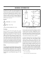
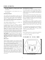
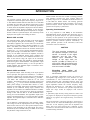
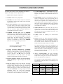
INSTRUCTION
MANUAL
SPECTRUM ANALYZERS
MODELS
2165A
2620A
2625
2630
TEST INSTRUMENT SAFETY
1. Some equipment with a two-wire ac power cord,
including some with polarized power plugs, is the
“hot chassis” type. This includes most recent
television receivers and audio equipment. A plastic or
wooden cabinet insulates the chassis to protect the
customer. When the cabinet is removed for servicing,
a serious shock hazard exists if the chassis is touched.
Not only does this present a dangerous shock hazard,
but damage to test instruments or the equipment under
test may result from connecting the ground lead of
most test instruments to a “hot chassis”. To test “hot
chassis” equipment, always connect an isolation
transformer between the ac outlet and the equipment
under test. The B+K Precision Model TR-110
Isolation Transformer, or Model 1653A or 1655A AC
Power Supply is suitable for most applications. To be
on the safe side, treat all two-wire ac equipment as
“hot-chassis” unless you are sure it has an isolated
chassis or an earth ground chassis.
Normal use of test equipment exposes you to a certain
amount of danger from electrical shock because testing
must sometimes be performed where exposed voltage is
present. An electrical shock causing 10 milliamps of
current to pass through the heart will stop most human
heartbeats. Voltage as low as 35 volts dc or ac rms should
be considered dangerous and hazardous since it can
produce a lethal current under certain conditions. Higher
voltages pose an even greater threat because such voltage
can more easily produce a lethal current. Your normal
work habits should include all accepted practices to
prevent contact with exposed high voltage, and to steer
current away from your heart in case of accidental contact
with a high voltage. You will significantly reduce the risk
factor if you know and observe the following safety
precautions:
5. Don’t expose high voltage needlessly. Remove
housings and covers only when necessary. Turn off
equipment while making test connections in highvoltage circuits. Discharge high-voltage capacitors
after removing power.
2. On test instruments or any equipment with a 3-wire ac
power plug, use only a 3-wire outlet. This is a safety
feature to keep the housing or other exposed elements
at earth ground.
6. If possible, familiarize yourself with the equipment
being tested and the location of its high voltage
points. However, remember that high voltage may
appear at unexpected points in defective equipment.
3. B+K Precision products are not authorized for use in
any application involving direct contact between our
product and the human body, or for use as a critical
component in a life support device or system. Here,
“direct contact” refers to any connection from or to
our equipment via any cabling or switching means. A
“critical component” is any component of a life
support device or system whose failure to perform can
be reasonably expected to cause failure of that device
or system, or to affect its safety or effectiveness.
7. Use an insulated floor material or a large, insulated
floor mat to stand on, and an insulated work surface
on which to place equipment; and make certain such
surfaces are not damp or wet.
8. Use the time proven “one hand in the pocket”
technique while handling an instrument probe. Be
particularly careful to avoid contacting a nearby
metal object that could provide a good ground return
path.
4. Never work alone. Someone should be nearby to
render aid if necessary. Training in CPR (cardiopulmonary resuscitation) first aid is highly
recommended.
9. When testing ac powered equipment, remember that
ac line voltage is usually present on some power
input circuits such as the on-off switch, fuses, power
transformer, etc. any time the equipment is connected
to an ac outlet, even if the equipment is turned off.
2
Instruction Manual
for
Models
2615A, 2620A, 2625, 2630
SPECTRUM ANALYZERS
3
TABLE OF CONTENTS
Page
Page
TEST INSTRUMENT SAFETY ..... Inside front cover
INTRODUCTION TO SPECTRUM ANALYSIS.... 17
SPECIFICATIONS .................................................... 5
General .................................................................. 17
OPTIONAL ACCESSORIES .................................... 6
Types of Spectrum Analyzers ................................. 17
GENERAL INFORMATION..................................... 7
Spectrum Analyzer Requirements ........................... 18
Symbols .................................................................. 7
Frequency Measurements ....................................... 18
Tilt handle................................................................ 7
Resolution.............................................................. 18
Safety....................................................................... 7
Sensitivity .............................................................. 19
Operating Conditions................................................ 8
Maintenance............................................................. 8
Video Filtering ....................................................... 19
Selecting the Line Voltage........................................ 8
Spectrum Analyzer Sensitivity................................ 19
INTRODUCTION...................................................... 9
Frequency Response............................................... 20
General .................................................................... 9
Tracking Generators ............................................... 20
Operating Considerations ......................................... 9
APPENDIX–dBm CONVERSION .......................... 22
CONTROLS AND INDICATORS ........................... 10
CUSTOMER SUPPORT.......................................... 23
CALIBRATION ....................................................... 15
INSTRUMENT REPAIR SERVICE ....................... 23
Vertical Calibration ................................................ 15
Horizontal Calibration ............................................ 15
WARRANTY SERVICE INSTRUCTIONS ............ 24
LIMITED ONE-YEAR WARRANTY..................... 25
4
SPECIFICATIONS
Frequency
Input
Frequency range:
0.15 MHz to 1050 MHz (–3 dB) (Models 2625 and 2630)
0.15 MHz to 500 MHz (–3 dB) (Models 2615A and
2620A)
Center frequency display accuracy: ±100 kHz
Marker accuracy: ±(0.1% span + 100 kHz)
Frequency display resolution: 100 kHz
(4½ digit LED for Models 2625 and 2630)
(4 digit LED for Models 2615A and 2620A)
Frequency scanwidth:
100 kHz/div. to 100 MHz/div. (Models 2625 and 2630)
in 1-2-5 steps and 0 Hz/div. (Zero Scan)
50 kHz/div. to 50 MHz/div. (Models 2615A and 2620A)
in 1-2-5 steps and 0 Hz/div. (Zero Scan)
Frequency scanwidth accuracy: ±10%
Frequency stability: Drift: <150 kHz / hour
IF-Bandwidth (–3 dB):
Resolution: 400 kHz and 20 kHz
(Models 2625 and 2630)
Resolution: 250 kHz and 20 kHz
(Models 2615A and 2620A)
Video-Filter on: 4 kHz
Sweep rate: 43 Hz
Input impedance: 50?
Input connector: BNC
Input attenuator: 0 to 40 dB (4 x 10 dB steps)
Input attenuator accuracy: ±1 dB/10 dB step
Max. input level: +10 dBm, ±25VDC (0 dB attenuation)
+20 dBm (40 dB attenuation)
Tracking Generator (Models 2620A and 2630
only)
Output level range: –50 dBm to +1 dBm
(in 10 dB steps and variable)
Output attenuator: 0 to 40 dB (4 x 10 dB steps)
Output attenuator accuracy: ±l dB
Output impedance: 50? (BNC)
Frequency range:
0.15 MHz to 1050 MHz (Model 2630)
0.1 MHz to 500 MHz (Model 2620A)
Frequency response: ±1.5 dB
Radio Frequency Interference (RFI): <20 dBc
General
Display: CRT, 6 inch, 8 x 10 div. internal graticule
Trace rotation: Adjustable on front panel
Output Probe Power: 6V
Line voltage: 115 / 230V ±10%, 50-60Hz
Power consumption: approx. 27W
Operating ambient temperature:
+10°C to +40°C
Protective system: Safety Class I (IEC 1010-1)
Weight:
Approx. 15.4 lb. (6 kg) (Models 2625 and 2630)
Approx. 13.2 lb. (5 kg) (Models 2615A and 2620A)
Dimensions:
4.9 in. (125 mm) H x 11.2 in. (285mm) W x 15 in. (380
mm) D.
Amplitude
Amplitude range: –100 dBm to +13 dBm
Screen display range: 80 dB (10 dB / div.)
Reference level: –27 dBm to +13 dBm
(in 10 dB steps)
Reference level accuracy: ±2 dB
Average noise level:
–99 dBm (20 kHz BW) (Models 2625 and 2630)
–99 dBm (20 kHz BW) (Models 2615A and 2620A)
Distortion:
<–75 dBc; 2nd and 3rd harmonic
3rd order intermod.: –70 dBc
(two signals >3 MHz apart)
Sensitivity: dB above average noise level
Log scale fidelity: ±2 dB (without attn.) Ref.: 250 MHz
IF gain: 10 dB adjustment range
Accessories Supplied
Power Cord
Instruction Manual
NOTE: Specifications and information are subject to change without notice. Please visit www.bkprecision.com for the most current product
information.
5
OPTIONAL ACCESSORIES
Near Field “Sniffer” Probe Set; Model PR-261
Antenna Kit; Model AN-18
The PR-261 is the ideal tool kit for the investigation of
RF electromagnetic fields. It is indispensable for EMI
pre-compliance testing during product development, prior
to third party testing. The set includes three hand-held
probes with a built-in pre-amplifier covering the
frequency range from 10 kHz to 1000 MHz. The set
includes one magnetic field probe, one electric field probe
and one high impedance probe. All have high sensitivity
and are matched to the 50? inputs of spectrum analyzers.
The power can be supplied either from the batteries or
through a power cord directly connected to a B+K
Precision Models 2615A, 2620A, 2625 and 2630. Signal
feed is via a 1.5 meter BNC-cable. When used in conjunction with a spectrum analyzer, the probes can be used to
locate and qualify EMI sources. They are especially suited
to locate emission “hot spots” on PCBs and cables, as
well as evaluate EMC problems at the breadboard and
prototype level. They enable the user to evaluate radiated
fields and perform shield effectivity comparisons.
Mechanical screening performance and immunity tests on
cables and components are easily performed. Faulty
components and poor bonding locations can be isolated.
Broad band antenna is useful for radiated signal
measurement.
Deluxe Carrying Case; Model LC-210
Rugged cordura carrying case is foam padded for
instrument protection, has zipped pockets for manual and
accessories, and includes web hand strap and shoulder
strap.
Viewing Hood; Model VH-26
Shades CRT to block ambient light and improve
definition of the display.
50-ohm to 75-ohm Matching Network;
Model ZTF-1
Most RF networks (except cable TV) have an impedance
of 50 ohms. The spectrum analyzers also have a 50 ohm
input impedance, which allows direct connection. Cable
TV networks have an impedance of 75 ohms. To use the
spectrum analyzer with 75 ohm networks, Model ZTF-1
will match the 75 ohm network to the 50 ohm input
impedance of the spectrum analyzer.
The magnetic probe incorporates a high degree of
rejection of both stray and direct electric fields, and
provides far greater repeatability than with conventional
field probes. Measurements can be made on the very near
field area that is close to components or radiation sources.
The electric field (monopole) probe has the highest
sensitivity of all three probes. It can be used to check
screening and perform pre-compliance testing on a
comparative basis. The high impedance probe is used to
measure directly on the components under test or at the
conductive trace of a PC board. It has an input
capacitance of only 2 pF and supplies virtually no
electrical charge to the device under test.
50-ohm Feedthru Termination; Model TE-26
The output levels of the tracking generator of the Models
2620 and 2630 are correct only when terminated into 50
ohms. The Model TE-26 provides a 50 ohm termination
and a BNC feedthru connection so that the tracking
generator output may be fed into high impedance circuit
at a calibrated level.
Rack Mount Adapter; Model RM-26
Probe Set Specifications
Model RM-26 mounts the spectrum analyzer to standard
19-inch racks.
All probes are electrically shielded and are supplied in a
carrying case.
Frequency range: 100 kHz–1,2GHz
Power supply: 6V from Spectrum Analyzers or Batteries
Operating current: 10-15 mA
Probe dimensions: 40 x 19 x 195 mm (approx.)
6
GENERAL INFORMATION
The Models 2615A, 2620A, 2625, and 2630 spectrum analyzers are easy to operate. The logical arrangement of the
controls allows anyone to quickly become familiar with the
operation of the instrument, however, experienced users are
also advised to read through these instructions so that all
functions are understood. Immediately after unpacking, the
instrument should be checked for mechanical damage and
loose parts in the interior. If there is transport damage, the
supplier must be informed immediately. The instrument must
then not be put into operation.
Symbols
ATTENTION - refer to manual
Danger - High voltage
Protective ground (earth) terminal
Fig. 1. Tilt Handle Operation
Tilt handle
The case, chassis and all measuring terminals are connected
to the protective earth contact of the appliance inlet. The
instrument operates according to Safety Class I (three-conductor power cord with protective earthing conductor and
a plug with earthing contact). The mains/line plug shall only
be inserted in a socket outlet provided with a protective earth
contact. The protective action must not be negated by the use
of an extension cord without a protective conductor.
To view the screen from the best angle, there are three
different positions (C, D, E) for setting up the instrument
(see Figure 1). If the instrument is set down on the floor
after being carried, the handle automatically remains in the
upright carrying position (A). In order to place the
instrument onto a horizontal surface, the handle should be
turned to the upper side of the Spectrum Analyzer (C). For
the D position (10° inclination), the handle should he turned
to the opposite direction of the carrying position until it
locks in place automatically underneath the instrument. For
the E position (20° inclination), the handle should be pulled
to release it from the D position and swing backwards until it
locks once more. The handle may also be set to a position
for horizontal carrying by turning it to the upper side to lock
in the B position. At the same time, the instrument must be
lifted, because otherwise the handle will jump back.
The mains/line plug should be inserted before connections
are made to measuring circuits. The grounded accessible
metal parts (case, sockets, jacks) and the mains/line supply
contacts (line/live, neutral) of the instrument have been
tested against insulation breakdown with 2200V DC. Under
certain conditions, 50 Hz or 60 Hz hum voltages can occur in
the measuring circuit due to the interconnection with other
mains/line powered equipment or instruments. This can be
avoided by using an isolation transformer (Safety Class II)
between the mains/line outlet and the power plug of the
device being investigated. Most cathode-ray tubes develop
X-rays. However, the dose equivalent rate falls far below
the maximum permissible value of 36pA/kg (0.5mR/h).
Whenever it is likely that protection has been impaired, the
instrument shall be made inoperative and be secured against
any unintended operation. The protection is likely to be
impaired if, for example:
Safety
This instrument has been designed and tested in accordance
with IEC Publication 1010-1, Safety requirements for electrical equipment for measurement, control, and laboratory
use. The CENELEC regulations EN 61010-1 correspond to
this standard. It has left the factory in a safe condition. This
instruction manual contains important information and warnings which have to be followed by the user to ensure safe
operation and to retain the Spectrum Analyzer in a safe
condition.
• shows visible damage
• fails to perform the intended measurements
7
GENERAL INFORMATION
• has been subjected to prolonged storage under
unfavorable conditions (e.g. in the open or in moist
environments)
Selecting the Line Voltage
The spectrum analyzer operates at mains/line voltages of
115V AC and 230V AC. The voltage selection switch is
located on the rear of the instrument and displays the
selected voltage. The correct voltage can be selected using a
small screwdriver.
• has been subjected to severe transport stress (e.g. in
poor packaging).
Operating Conditions
Remove the power cable from the power connector prior to
making any changes to the voltage setting. The fuses must
also be replaced with the appropriate value (see Fuse Type)
prior to connecting the power cable. Both fuses are
externally accessible by removing the fuse cover located
above the 3-pole power connector.
The instrument has been designed for indoor use. The
permissible ambient temperature range during operation is
+10°C (+50°F) to +40°C (+104°F). It may occasionally be
subjected to temperatures between +10°C (+50°F) and –
10°C (+14°F) without degrading its safety. The permissible
ambient temperature range for storage or transportation is –
40°C (+14°F) to +70°C (+158°F).
The fuseholder can be released by pressing its plastic
retainers with the aid of a small screwdriver (see Figure 2).
The retainers are located on the right and left side of the
holder and must be pressed towards the center. The fuse(s)
can then be replaced and pressed in until locked on both
sides.
The maximum operating altitude is up to 2200m. The
maximum relative humidity is up to 80%.
If condensed water exists in the instrument it should be
acclimatized before switching on. In some cases (e.g.
instrument extremely cold) two hours should be allowed
before the instrument is put into operation. The instrument
should be kept in a clean and dry room and must not be
operated in explosive, corrosive, dusty, or moist
environments. The spectrum analyzer can be operated in any
position, but the convection cooling must not be impaired.
For continuous operation the instrument should be used in
the horizontal position, preferably tilted upwards, resting on
the tilt handle.
The specifications stating tolerances are only valid if the
instrument has warmed up for 60 minutes at an ambient
temperature between +15°C (+59°F) and +30°C (+86°F).
Values without tolerances are typical for an average
instrument.
Use of patched fuses or short-circuiting of the fuseholder is
not permissible; B+K Precision assumes no liability
whatsoever for any damage caused as a result, and all
warranty claims become null and void.
Fuse type:
Size 5 x 20 mm; 250-Volt AC; must meet IEC specification
127, Sheet III (or DIN 41 662 or DIN 41 571, sheet 3).
Time characteristic: time-lag
Line voltage 115V~ ±10%:
Line voltage 230V~ ±10%:
Fuse rating:
Fuse rating:
Maintenance
Various important properties of the spectrum analyzer
should be carefully checked at certain intervals. Only in this
way it is certain that all signals are displayed with the
accuracy on which the technical data are based.
The exterior of the instrument should be cleaned regularly
with a dusting brush. Dirt which is difficult to remove on the
casing and handle, the plastic and aluminum parts, can be
removed with a moistened cloth (99% water + 1% mild
detergent). Spirit or washing benzene (petroleum ether) can
be used to remove greasy dirt.
The screen may be cleaned with water or washing benzene
(but not with spirit (alcohol) or solvents), it must then be
wiped with a dry clean lint-free cloth. Under no
circumstances may the cleaning fluid get into the instrument.
The use of other cleaning agents can attack the plastic and
paint surfaces.
Fig. 2. Fuse Replacement
8
T 315mA
T 160mA
INTRODUCTION
General
Models 2620A and 2630 each include a tracking generator.
This generator provides sine wave voltages within the
frequency range of 0.1 to 1050 MHz for Model 2630 and 0.1
to 500 MHz for Model 2620A. The tracking generator
frequency is determined by the first oscillator (1st LO) of the
spectrum analyzer section. Spectrum analyzer and tracking
generator are frequency synchronized.
The spectrum analyzer permits the detection of spectrum
components of electrical signals in the frequency range of 0.15
to 1050 MHz for Models 2625 and 2630 and 0.15 to 500 MHz
for Models 2615 and 2620. The detected signal and its content
have to be repetitive. In contrast to an oscilloscope operated in
Yt mode, where the amplitude is displayed on the time domain,
the spectrum analyzer displays amplitude on the frequency
domain (Yf). The individual spectrum components of “a signal”
become visible on a spectrum analyzer. The oscilloscope would
display the same signal as one resulting waveform.
Operating Considerations
It is very important to read Safety in the GENERAL
INFORMATION Section including the instructions prior to
operating the spectrum analyzer. No special knowledge is
necessary for the operation of the spectrum analyzer. The
straightforward front panel layout and the limitation to basic
functions guarantee efficient operation immediately. To
ensure optimum operation of the instrument, some basic
instructions need to be followed.
Models 2625 and 2630
The spectrum analyzer works according to the triple superhet
receiver principle. The signal to be measured (fin = 0.15 MHz to
1050 MHz) is applied to the 1st mixer where it is mixed with
the signal of a variable voltage controlled oscillator (fLO 1350
MHz – 2350 MHz). This oscillator is called the lst LO (local
oscillator). The difference between the oscillator and the input
frequency (fLO – fin = 1st IF) is the first intermediate frequency,
which passes through a waveband filter tuned to a center frequency of 1350 MHz. It then enters an amplifier, and this is
followed by two additional mixing stages, oscillators and
amplifiers. The second IF is 29.875 MHz and the third is 2.75
MHz. In the third IF stage, the signal can be selectively
transferred through a filter with 400 kHz or 20 kHz bandwidth
before arriving at an AM demodulator. The logarithmic output
(video signal) is transferred directly, or via a low pass filter to
another amplifier. This amplifier output is connected to the Y
deflection plates of the CRT.
CAUTION
The most sensitive component of
the spectrum analyzer is the input
section. It consists of the signal
attenuator and the first mixer.
Without input attenuation, the
voltage at the input must not
exceed +10 dBm (0.7Vrms) AC or
±25 volt DC. With a maximum input
attenuation of 40 dB the AC voltage
must not exceed +20 dBm.
Exceeding
these
limits
will
damage the input attenuator and/or
the first mixer.
Models 2615A and 2620A
The spectrum analyzer works according to the triple superhet
receiver principle. The signal to be measured (fin = 0.5 MHz to
500 MHz) is applied to the 1st mixer where it is mixed with the
signal of a variable voltage controlled oscillator (fLO 610 MHz –
1110 MHz). This oscillator is called the 1st LO (local
oscillator). The difference between the oscillator and the input
frequency (fLO – fin = 1st IF) is the first intermediate frequency,
which passes through a waveband filter tuned to a center
frequency of 609.5 MHz. It then enters an amplifier, and this is
followed by two additional mixing stages, oscillators and
amplifiers. The second IF is 29.5 MHz and the third is 2.9 MHz.
In the third IF stage, the signal can be selectively transferred
through a filter with 250 kHz or 20 kHz bandwidth before
arriving at an AM demodulator. The logarithmic output (video
signal) is transferred directly, or via a low pass filter to another
amplifier. This amplifier output is connected to the Y deflection
plates of the CRT.
Prior to examining unidentified signals, the presence of
unacceptable high voltages has to be checked. It is also
recommended to start measurements with the highest
possible attenuation and a maximum frequency range. The
user should also consider the possibility of excessively high
signal amplitudes outside the covered frequency range,
although not displayed (e.g. 1200 MHz). The frequency
range of 0 Hz to 150 kHz is not specified. Spectral lines
within this range would be displayed with incorrect
amplitude.
A particularly high intensity setting shall be avoided. The
way signals are displayed on the spectrum analyzer typically
allows for any signal to be recognized easily, even with low
intensity.
Due to the frequency conversion principle, a spectral line is
visible at 0 Hz. It is called IF-feedthrough. The line appears
when the 1st LO frequency passes the IF amplifiers and
filters. The level of this spectral line is different in each
instrument. A deviation from the full screen does not indicate
a malfunctioning instrument.
The X deflection is performed with a ramp generator voltage.
This voltage can also be superimposed on a dc voltage which
allows for the control of 1st LO. The spectrum analyzer scans a
frequency range depending on the ramp height. This span is
determined by the scanwidth setting. In ZERO SCAN mode
only the direct voltage controls the 1st LO.
9
CONTROLS AND INDICATORS
1. CENTER FREQUENCY – Coarse/Fine. Both rotary
knobs are used for center frequency setting. The center
frequency is displayed at the horizontal center of the
screen.
The front panel controls of the instruments are shown in
Figures 3 through 6 and are explained below.
7. FOCUS. Beam sharpness adjustment.
2. BANDWIDTH. Selects the IF bandwidth. When the
switch is engaged, the noise level decreases and the
selectivity is improved. Spectral lines which are
relatively close together can be distinguished. As the
small signal transient response requires a longer time,
this causes incorrect amplitude values if the scanwidth
is set at too wide a frequency span. The UNCAL LED
will indicate this condition.
8. INTENS. Beam intensity adjustment.
9. POWER (Power ON and OFF). If power is switched to
ON position, a beam will be visible on the screen after
approximately 10 sec..
10. TR (Trace Rotation). Despite Mumetal-shielding of
the CRT, effects of the earth’s magnetic field on the
horizontal trace position cannot be completely avoided.
A potentiometer accessible through an opening can be
used for correction. Slight pincushion distortion is
unavoidable and cannot be corrected.
3. VIDEO FILTER. The video filter may be used to
reduce noise on the screen. It enables small level
spectral lines to become visible which normally would
be within or just above the medium noise level. The
filter bandwidth is 4 kHz.
11. MARKER - ON/OFF switch. When the MARKER
pushbutton is set to the OFF position, the CF indicator
is lit and the display shows the center frequency. When
the switch is in the ON position, MK is lit and the
display shows the marker frequency. The marker is
shown on the screen as a sharp peak. The marker
frequency is adjustable by means of the MARKER
knob and can be aligned with a spectral line.
4. Y-POS. Control for adjusting the vertical beam
position.
5. INPUT. The BNC 50? input of the spectrum analyzer.
Without input attenuation the maximum permissible
input voltages of ±25V DC and +l0 dBm AC must not
be exceeded. With the maximum input attenuation of
40 dB the maximum input voltage is +20 dBm.
NOTE
The maximum dynamic range of the instrument is 70
dB. Higher input voltages exceeding the reference level
cause signal compression and intermodulation. Those
effects will lead to erroneous displays. If the input
level exceeds the reference level, the input level
attenuation must be increased.
Switch off the marker before taking
correct amplitude readings.
12. CF/MK (CENTER FREQUENCY/ MARKER)
indicator. The CF LED is lit when the digital display
shows the center frequency. The center frequency is
the frequency which is displayed in the horizontal
center of the CRT. The MK LED is lit when the
Marker pushbutton is in the ON position. The digital
display shows the marker frequency in that case.
6. ATTN. (ATTENUATOR). The Input Attenuator
consists of four 10 dB attenuators, reducing the signal
height before entering the 1st mixer. Each attenuator is
active if the push button is depressed.
13. DIGITAL DISPLAY (Display of Center Frequency/
Marker Frequency) 7-segment display with 100 kHz
resolution.
The correlation of selected attenuation, reference level
and baseline level (noise level) is according to the
following listing:
14. UNCAL. Blinking of this LED indicates incorrectly
displayed amplitude values. This is due to scanwidth
and filter setting combinations which give uncalibrated
amplitude readings because the IF-filters have not
settled. This may occur when the scanned frequency
range (SCANWIDTH) is too large compared to the IF
bandwidth, and/or the video filter bandwidth.
Measurements in this case can either be taken without
a video filter or the scanwidth has to be decreased.
Attenuation
10
Reference level
Base line
0 dB
–27 dBm
10 mV
–107 dBm
10 dB
–17 dBm
31.6 mV
–97 dBm
20 dB
–7 dBm
0.1 V
–87 dBm
30 dB
+3 dBm
316 mV
–77 dBm
40 dB
+13 dBm
1V
–67 dBm
CONTROLS AND INDICATORS
Fig. 3. Model 2615A Front Panel
Fig. 4. Model 2620A Front Panel
The reference level is represented by the upper
horizontal graticule line. The lowest horizontal
graticule line indicates the baseline. The vertical
graticule is subdivided in 10 dB steps.
As previously pointed out, the maximum permissible input
voltages may not be exceeded. This is extremely important
because it is possible that the spectrum analyzer will only
show a partial spectrum of currently applied signals.
11
CONTROLS AND INDICATORS
Fig. 5. Model 2625 Front Panel
Fig. 6. Model 2630 Front Panel
Consequently, input signals might be applied
with excessive levels outside the displayed
frequency range leading to the destruction of
the input attenuator and/or the 1st mixing stage.
Also refer to INPUT.
The highest attenuation (4 x 10 dB) and the highest
usable frequency range (highest scanwidth setting)
should be selected prior to connecting any signal to the
input.
12
CONTROLS AND INDICATORS
The center frequency is indicated by the vertical
graticule line at middle of the horizontal axis. If the
center frequency and the scanwidth setting are correct,
the X axis has a length of 10 divisions. On scanwidth
settings lower than 50 MHz, only a part of the entire
frequency range is displayed.
This permits the detection of any spectral lines which are
within the maximum measurable and displayable
frequency range, if the center frequency is set to 500 MHz
for Models 2625 and 2630 or 250 MHz for Models 2615A
and 2620A. If the baseline tends to move upwards when
the attenuation is decreased, it may indicate spectral lines
outside the maximum displayable frequency range with
excessive amplitude.
When SCANWIDTH is set to 50 MHz/div. and if center
frequency is set to 250 MHz, the displayed frequency
range extends to the right by 50 MHz per division,
ending at 500 MHz (250 MHz + (5 x 50 MHz)). The
frequency decreases to the left in a similar way. In this
case the left graticule line corresponds to 0 Hz.
15. SCANWIDTH (Models 2625 and 2630). The
SCANWIDTH selectors allow to control the scanwidth
per division of the horizontal axis. The frequency/Div. can
be increased by means of the ? button, and decreased by
means of the ? button. Switching is accomplished in 1-25 steps from 100 kHz/div. to 100 MHz/div.
With these settings, a spectral line is visible which is
referred to as “Zero Frequency”. It is the 1st LO
(oscillator) which becomes visible when its frequency
passes the first IF filter. This occurs when the center
frequency is low relative to the scanwidth range
selected. The “Zero Frequency” is different in level in
every instrument and therefore cannot be used as a
reference level. Spectral lines displayed left of the
“Zero Frequency Point” are so called image
frequencies.
The width of the scan range is displayed in MHz/div. and
refers to each horizontal division on the graticule. The
center frequency is indicated by the vertical graticule line
at middle of the horizontal axis. If the center frequency
and the scanwidth setting are correct, the X axis has a
length of 10 divisions. On scanwidth settings lower than
100 MHz, only a part of the entire frequency range is
displayed.
In the ZERO SCAN mode the spectrum analyzer
operates like a receiver with selectable bandwidth. The
frequency is selected via the CENTER FREQ. knob.
Spectral line(s) passing the IF filter cause a level
display (selective voltmeter function).
When SCANWIDTH is set to 100 MHz/div. and if center
frequency is set to 500 MHz, the displayed frequency
range extends to the right by 100 MHz per division,
ending at 1000 MHz (500 MHz + (5 x 100 MHz)). The
frequency decreases to the left in a similar way. In this
case the left graticule line corresponds to 0 Hz.
The selected scanwidth/div. settings are indicated by a
number of LEDs above the range setting push buttons.
With these settings, a spectral line is visible which is
referred to as “Zero Frequency”. It is the 1st LO
(oscillator) which becomes visible when its frequency
passes the first IF filter. This occurs when the center
frequency is low relative to the scanwidth range selected.
The “Zero Frequency” is different in level in every
instrument and therefore cannot be used as a reference
level. Spectral lines displayed left of the “Zero Frequency
Point” are so called image frequencies.
15. X-POS. (X-position).
16. X-AMPL. (X-amplitude).
IMPORTANT: These controls are only necessary when
calibrating the instrument. They do not require adjustment
under normal operating conditions. A very accurate RF
Generator is necessary if any adjustment of these controls
is required.
In the ZERO SCAN mode the spectrum analyzer operates
like a receiver with selectable bandwidth. The frequency is
selected via the CENTER FREQ. knob. Spectral line(s)
passing the IF filter cause a level display (selective
voltmeter function).
17. PHONE (3.5 mm earphone connector). An earphone
or loudspeaker with an impedance >16 Ohms can be
connected to this output. When tuning the spectrum
analyzer to a spectral line possibly available audio
signals can be detected. The signal is provided by an
AM-Demodulator in the IF-section. It demodulates any
available AM-Signal and provides as well one-side FMDemodulation. The output is short circuit proof.
The selected scanwidth/div. settings are indicated by a
number of LEDs above the range setting push buttons.
20. SCANWIDTH (Models 2615A and 2620A). The
SCANWIDTH selectors allow to control the scanwidth
per division of the horizontal axis. The frequency/Div. can
he increased by means of the ? button, and decreased by
means of the ? button. Switching is accomplished in 1-25 steps from 50 kHz/div. to 50 MHz/div.
18. VOLUME. Volume setting for earphone output.
19. PROBE POWER. The output provides a +5 Vdc
voltage for the operation of an PR-261 near field sniffer
probe. It is only provided for this purpose and requires
a special cable which is shipped along with the PR-261
probe set.
The width of the scan range is displayed in MHz/div. and
refers to each horizontal division on the graticule.
13
CONTROLS AND INDICATORS
TRACKING GENERATOR CONTROLS
(Models 2620A and 2630)
21. TRACK GEN. The tracking generator is activated
when this button is engaged. When activated, a sine
signal can be obtained at the OUTPUT BNC
connector at a frequency determined by the spectrum
analyzer. In ZERO SCAN mode, the center
frequency appears at the output.
23. ATTN. (ATTENUATOR). Output level attenuator
with four 10 dB attenuators which allow the signal
to be reduced prior to reaching the OUTPUT jack.
The four attenuators are equal and each is activated
by depressing the button. When engaged, each
provides a 10 dB attenuation. Any combination of
buttons may be used to achieve the desired
attenuation.
24. OUTPUT. 50?
generator.
22. LEVEL. This knob adjusts the level of the tracking
generator. Continuously variable from –10 dBm to
+l dBm; operates in conjunction with step
attenuators for +1 dBm to –50 dBm output level.
BNC output of the tracking
14
CALIBRATION
Vertical Calibration (Models 2625 and 2630)
A: A single spectral line (–27 dBm) appears on the screen.
The spectral line maximum is now adjusted with the Y-POS.
control (12) and placed at the top graticule line of the screen.
All input attenuators switches have to be released.
Prior to calibration, ensure that all input attenuators (14) are
released. The spectrum analyzer must be in operation for at
least 60 minutes prior to calibration. Switch VIDEO
FILTER (11) to OFF position. Set BANDWIDTH (10) to
400 kHz. Set SCANWIDTH (15) to 2 MHz/div.
B: Next, the generator signal must be switched back and
forth between –27 dBm and –77 dBm, and the Y-AMPL.
control adjusted so that the spectral line peak changes by 5
divisions in the vertical direction. If this results in a change
of the Y-position, the calibration outlined under A has to be
repeated. The calibrations A and B have to be repeated until
an ideal adjustment is achieved.
Connect calibrated RF signal of –27 dBm ±0.2 dB (10 mV)
to the spectrum analyzer input (13). The frequency of this
signal should be between 2 MHz and 250 MHz. Set the
center frequency to the signal frequency.
Finally, the operation of the input attenuators (14) can be
tested at a level of –27 dBm. The spectral line visible on the
screen can be reduced in 4 steps of 10 dB each by activating
the attenuators incorporated in the spectrum analyzer. Each
10 dB step corresponds to one graticule division on the
screen. The tolerance may not exceed ±l dB in all attenuation
positions.
A: A single spectral line (–27 dBm) appears on the screen.
The spectral line maximum is now adjusted with the Y-POS.
control (12) and placed at the top graticule line of the
screen. All input attenuators switches have to be released.
The following adjustment is only necessary for service
purposes and if the check of this settings shows deviations
of the correct settings. The y-ampl. control is located on the
XY-PCB inside the instrument. In case any adjustment of
the vertical amplification is necessary, please refer to the
service manual.
Horizontal Calibration (Models 2625 and 2630)
Prior to calibration ensure that all input attenuators switches
(14) are released. The spectrum analyzer must be operated
for at least 60 minutes prior to calibration. The VIDEO
FILTER push button (11) must be in OFF position. Set
BANDWIDTH (10) to 400 kHz. Set the SCANWIDTH (15)
to 50 MHz/div. After the center frequency is set to 250 MHz,
a generator signal must be applied to the input. The output
level should be between 40 and 50 dB above the noise.
B: Next, the generator signal must be switched back and
forth between –27 dBm and –77 dBm, and the Y-AMPL.
control adjusted so that the spectral line peak changes by 5
divisions in the vertical direction. If this results in a change
of the Y-position, the calibration outlined under A has to be
repeated. The calibrations A and B have to be repeated until
an ideal adjustment is achieved.
C: Set generator frequency to 250 MHz. Adjust the peak of
the 250 MHz spectral line to the horizontal screen center
using the X-POS. control (16).
Finally, the operation of the input attenuators (14) can be
tested at a level of –27 dBm. The spectral line visible on the
screen can be reduced in 4 steps of 10 dB each by activating
the attenuators incorporated in the spectrum analyzer. Each
10 dB step corresponds to one graticule division on the
screen. The tolerance may not exceed ±1 dB in all
attenuation positions.
D: Set the generator frequency to 50 MHz. If the 50 MHz
spectral line is not on the second graticule line from left, it
should be aligned using the X-AMPL. control (17). Then the
calibration as described under C should be verified and
corrected if necessary.
Vertical Calibration (Models 2615A and 2620A)
The calibrations C and D should be repeated until optimum
adjustment is achieved.
Prior to calibration, ensure that all input attenuators (14) are
released. The spectrum analyzer must be in operation for at
least 60 minutes prior to calibration. Switch VIDEO
FILTER (11) to OFF position. Set BANDWIDTH (10) to
250 kHz. Set SCANWIDTH (15) to 2 MHz/div.
Horizontal Calibration (Models 2615A and 2620A)
Prior to calibration ensure that all input attenuators switches
(14) are released. The spectrum analyzer must be operated
for at least 60 minutes prior to calibration. The VIDEO
FILTER push button (11) must be in OFF position.
Connect calibrated RF signal of –27 dBm ±0.2 dB (10 mV)
to the spectrum analyzer input (13). The frequency of this
signal should be between 2 MHz and 250 MHz. Set the
center frequency to the signal frequency.
15
CALIBRATION
Set BANDWIDTH (10) to 250 kHz. Set the
SCANWIDTH (15) to 50 MHz/div. After the center
frequency is set to 250 MHz, a generator signal must be
applied to the input. The output level should be between
40 and 50 dB above the noise.
D: Set the generator frequency to 50 MHz. If the 50 MHz
spectral line is not on the 2nd. graticule line from left, it
should be aligned using the X-AMPL. control (17). Then
the calibration as described under C should be verified
and corrected if necessary.
C: Set generator frequency to 250 MHz. Adjust the peak
of the 250 MHz spectral line to the horizontal screen
center using the X-POS. control (16).
The calibrations C and D should be repeated until
optimum adjustment is achieved.
16
Introduction to Spectrum Analysis
General
The swept frequency responses of a filter or amplifier are
examples of swept frequency measurements possible with a
spectrum analyzer. These measurements are simplified by
using a tracking generator.
The analysis of electrical signals is a fundamental problem
for many engineers and scientists. Even if the immediate
problem is not electrical, the basic parameters of interest are
often changed into electrical signals by means of
transducers. The rewards for transforming physical
parameters to electrical signals are great, as many
instruments are available for the analysis of electrical signals
in the time and frequency domains.
Types of Spectrum Analyzers
There are two basic types of spectrum analyzers, swept-tuned
and real-time analyzers. The swept-tuned analyzers are tuned
by electrically sweeping them over their frequency range.
Therefore, the frequency components of a spectrum are
sampled sequentially in time. This enables periodic and
random signals to be displayed, but makes it impossible to
display transient responses. Real-time analyzers, on the other
hand, simultaneously display the amplitude of all signals in
the frequency range of the analyzer; hence the name realtime. This preserves the time dependency between signals
which permits phase information to be displayed. Real-time
analyzers are capable of displaying transient responses as
well as periodic and random signals.
The traditional way of observing electrical signals is to view
them in the time domain using an oscilloscope. The time
domain is used to recover relative timing and phase information which is needed to characterize electric circuit behavior.
However, not all circuits can be uniquely characterized from
just time domain information. Circuit elements such as
amplifiers, oscillators, mixers, modulators, detectors and
filters are best characterized by their frequency response
information. This frequency information is best obtained by
viewing electrical signals in the frequency domain. To
display the frequency domain requires a device that can
discriminate between frequencies while measuring the power
level at each. One instrument which displays the frequency
domain is the spectrum analyzer. It graphically displays
voltage or power as a function of frequency on a CRT
(cathode ray tube).
The swept-tuned analyzers are usually of the trf (tuned radio
frequency) or superheterodyne type. A trf analyzer consists
of a bandpass filter whose center frequency is tunable over a
desired frequency range, a detector to produce vertical
deflection on a CRT, and a horizontal scan generator used to
synchronize the tuned frequency to the CRT horizontal deflection. It is a simple, inexpensive analyzer with wide
frequency coverage, but lacks resolution and sensitivity.
Because trf analyzers have a swept filter they are limited in
sweep width depending on the frequency range (usually one
decade or less). The resolution is determined by the filter
bandwidth, and since tunable filters do not usually have
constant bandwidth, is dependent on frequency.
In the time domain, all frequency components of a signal are
seen summed together. In the frequency domain, complex
signals (i.e. signals composed of more than one frequency)
are separated into their frequency components, and the
power level at each frequency is displayed. The frequency
domain is a graphical representation of signal amplitude as a
function of frequency. The frequency domain contains
information not found in the time domain and therefore, the
spectrum analyzer has certain advantages compared with an
oscilloscope.
The most common type of spectrum analyzer differs from the
trf spectrum analyzers in that the spectrum is swept through a
fixed bandpass filter instead of sweeping the filter through
the spectrum. The analyzer is basically a narrowband
receiver which is electronically tuned in frequency by
applying a saw-tooth voltage to the frequency control
element of a voltage tuned local oscillator. This same sawtooth voltage is simultaneously applied to the horizontal
deflection plates of the CRT. The output from the receiver is
synchronously applied to the vertical deflection plates of the
CRT and a plot of amplitude versus frequency is displayed.
The analyzer is more sensitive to low level distortion than a
scope. Sine waves may look good in the time domain, but in
the frequency domain, harmonic distortion can be seen. The
sensitivity and wide dynamic range of the spectrum analyzer
is useful for measuring low-level modulation. It can be used
to measure AM, FM and pulsed RF. The analyzer can be
used to measure carrier frequency, modulation frequency,
modulation level, and modulation distortion. Frequency
conversion devices can be easily characterized. Such
parameters as conversion loss, isolation, and distortion are
readily determined from the display.
The analyzer is tuned through its frequency range by varying
the voltage on the LO (local oscillator).
The spectrum analyzer can be used to measure long and short
term stability. Parameters such as noise sidebands on an
oscillator, residual FM of a source and frequency drift during
warm-up can be measured using the spectrum analyzers
calibrated scans.
17
Introduction to Spectrum Analysis
It is important that the spectrum analyzer be more stable than
the signals being measured. The stability of the analyzer
depends on the frequency stability of its local oscillators.
Stability is usually characterized as either short term or long
term. Residual FM is a measure of the short term stability
which is usually specified in Hz peak-to-peak. Short term
stability is also characterized by noise sidebands which are a
measure of the analyzers spectral purity. Noise sidebands are
specified in terms of dB down and Hz away from a carrier in
a specific bandwidth. Long term stability is characterized by
the frequency drift of the analyzers LOs. Frequency drift is a
measure of how much the frequency changes during a
specified time (i.e., Hz/min. or Hz/hr).
The LO frequency is mixed with the input signal to produce
an IF (intermediate frequency) which can be detected and
displayed. When the frequency difference between the input
signal and the LO frequency is equal to the IF frequency, then
there is a response on the analyzer. The advantages of the
superheterodyne technique are considerable. It obtains high
sensitivity through the use of IF amplifiers, and many decades
in frequency can be tuned.
Also, the resolution can be varied by changing the bandwidth
of the IF filters. However, the superheterodyne analyzer is not
real-time and sweep rates must be consistent with the IF filter
time constant.
A peak at the left edge of the CRT is sometimes called the
“zero frequency indicator” or “local oscillator feedthrough”. It
occurs when the analyzer is tuned to zero frequency, and the
local oscillator passes directly through IF creating a peak on
the CRT even when no input signal is present. (For zero
frequency tuning, FLO=FIF). This effectively limits the lower
tuning limit.
Resolution
Before the frequency of a signal can be measured on a
spectrum analyzer it must first be resolved. Resolving a
signal means distinguishing it from its nearest neighbors. The
resolution of a spectrum analyzer is determined by its IF
bandwidth. The IF bandwidth is usually the 3 dB bandwidth
of the IF filter. The ratio of the 60 dB bandwidth (in Hz) to
the 3 dB bandwidth (in Hz) is known as the shape factor of
the filter. The smaller the shape factor, the greater is the
analyzers’ capability to resolve closely spaced signals of
unequal amplitude. If the shape factor of a filter is 15:1, then
two signals whose amplitudes differ by 60 dB must differ in
frequency by 7.5 times the IF bandwidth before they can be
distinguished separately. Otherwise, they will appear as one
signal on the spectrum analyzer display.
Spectrum Analyzer Requirements
To accurately display the frequency and amplitude of a signal
on a spectrum analyzer, the analyzer itself must be properly
calibrated. A spectrum analyzer properly designed for
accurate frequency and amplitude measurements has to satisfy
many requirements:
1.
2.
3.
4.
5.
6.
7.
Wide tuning range
Wide frequency display range
Stability
Resolution
Flat frequency response
High sensitivity
Low internal distortion
The ability of a spectrum analyzer to resolve closely spaced
signals of unequal amplitude is not a function of the IF filter
shape factor only. Noise sidebands can also reduce the
resolution. They appear above the skirt of the IF filter and
reduce the offband rejection of the filter. This limits the
resolution when measuring signals of unequal amplitude.
Frequency Measurements
The resolution of the spectrum analyzer is limited by its
narrowest IF bandwidth. For example, if the narrowest
bandwidth is 10 kHz, then the nearest any two signals can be
and still be resolved is 10 kHz. This is because the analyzer
traces out its own IF band-pass shape as it sweeps through a
CW signal. Since the resolution of the analyzer is limited by
bandwidth, it seems that by reducing the IF bandwidth
infinitely, infinite resolution will be achieved. The fallacy
here is that the usable IF bandwidth is limited by the stability
(residual FM) of the analyzer. If the internal frequency
deviation of the analyzer is 10 kHz, then the narrowest
bandwidth that can be used to distinguish a single input
signal is 10 kHz. Any narrower IF-filter will result in more
than one response or an intermittent response for a single
input frequency. A practical limitation exists on the IF
bandwidth as well, since narrow filters have long time
constants and would require excessive scan time.
The frequency scale can be scanned in three different modes
full, per division, and zero scan. The full scan mode is used to
locate signals because the widest frequency ranges are
displayed in this mode. (Not all spectrum analyzers offer this
mode.)
The per division mode is used to zoom-in on a particular
signal. In per division, the center frequency of the display is
set by the Tuning control and the scale factor is set by the
Frequency Span or Scan Width control. In the zero scan mode,
the analyzer acts as a fixed-tuned receiver with selectable
bandwidths.
Absolute frequency measurements are usually made from the
spectrum analyzer tuning dial. Relative frequency
measurements require a linear frequency scan. By measuring
the relative separation of two signals on the display, the
frequency difference can be determined.
18
Introduction to Spectrum Analysis
Sensitivity
Spectrum Analyzer Sensitivity
Sensitivity is a measure of the analyzers’ ability to detect
small signals. The maximum sensitivity of an analyzer is
limited by its internally generated noise. This noise is basically of two types: thermal (or Johnson) and nonthermal noise.
Thermal noise power can be expressed as:
Specifying sensitivity on a spectrum analyzer is somewhat
arbitrary. One way of specifying sensitivity is to define it as
the signal level when signal power = average noise power.
The analyzer always measures signal plus noise. Therefore,
when the input signal is equal to the internal noise level, the
signal will appear 3 dB above the noise. When the signal
power is added to the average noise power, the power level on
the CRT is doubled (increased by 3 dB) because the signal
power = average noise power.
PN = k x T x B
where:
PN = Noise power in watts
k
= Boltzmann’s Constant (1.38x10-23 Joule/K)
T
= absolute temperature, K
B
= bandwidth of system in Hertz
The maximum input level to the spectrum analyzer is the
damage level or burn-out level of the input circuit. This is +10
dBm for the input mixer and +20 dBm for the input attenuator.
Before reaching the damage level of the analyzer, the analyzer
will begin to gain compress the input signal. This gain
compression is not considered serious until it reaches 1 dB.
The maximum input signal level which will always result in
less than 1 dB gain compression is called the linear input level.
Above 1 dB gain compression the analyzer is considered to be
operating nonlinearly because the signal amplitude displayed
on the CRT is not an accurate measure of the input signal
level.
As seen from this equation, the noise level is directly
proportional to bandwidth. Therefore, a decade decrease in
bandwidth results in a 10 dB decrease in noise level and
consequently 10 dB better sensitivity. Nonthermal noise
accounts for all noise produced within the analyzer that is not
temperature dependent. Spurious emissions due to
nonlinearities of active elements, impedance mismatch, etc.
are sources of nonthermal noise. A figure of merit, or noise
figure, is usually assigned to this nonthermal noise which
when added to the thermal noise gives the total noise of the
analyzer system. This system noise which is measured on the
CRT, determines the maximum sensitivity of the spectrum
analyzer.
Whenever a signal is applied to the input of the analyzer,
distortions are produced within the analyzer itself. Most of
these are caused by the non-linear behavior of the input mixer.
These distortions are typically 70 dB below the input signal
level for signal levels not exceeding –27 dBm at the input of
the first mixer. To accommodate larger input signal levels, an
attenuator is placed in the input circuit before the first mixer.
The largest input signal that can be applied, at each setting of
the input attenuator, while maintaining the internally generated
distortions below a certain level, is called the optimum input
level of the analyzer. The signal is attenuated before the first
mixer because the input to the mixer must not exceed –27
dBm, or the analyzer distortion products may exceed the
specified 70 dB range. This 70 dB distortion-free range is
called the spurious-free dynamic range of the analyzer. The
display dynamic range is defined as the ratio of the largest
signal to the smallest signal that can be displayed
simultaneously with no analyzer distortions present.
Because noise level changes with bandwidth, it is important,
when comparing the sensitivity of two analyzers, to compare
sensitivity specifications for equal bandwidths.
A spectrum analyzer sweeps over a wide frequency range, but
is really a narrow band instrument. All of the signals that
appear in the frequency range of the analyzer are converted to
a single IF frequency which must pass through an IF filter; the
detector sees only this noise at any time. Therefore, the noise
displayed on the analyzer is only that which is contained in the
IF passband. When measuring discrete signals, maximum
sensitivity is obtained by using the narrowest IF bandwidth.
Video Filtering
Dynamic range requires several things then. The display range
must be adequate, no spurious or unidentified response can
occur, and the sensitivity must be sufficient to eliminate noise
from the displayed amplitude range.
Measuring small signals can be difficult when they are approximately the same amplitude as the average internal noise
level of the analyzer. To facilitate the measurement, it is best
to use video filtering. A video filter is a post-detection low
pass filter which averages the internal noise of the analyzer.
When the noise is averaged, the input signal may be seen. If
the resolution bandwidth is very narrow for the span, the video
filter should not be selected, as this will not allow the
amplitude of the analyzed signals to reach full amplitude due
to its video bandwidth limiting property.
The maximum dynamic range for a spectrum analyzer can be
easily determined from its specifications. First check the
distortion spec. For example, this might be “all spurious
products 70 dB down for –27 dBm at the input mixer”. Then,
determine that adequate sensitivity exists. For example, 70 dB
down from –27 dBm is –97 dB. This is the level we must be
able to detect, and the bandwidth required for this sensitivity
must not be too narrow or it will be useless. Last, the display
range must be adequate.
19
Introduction to Spectrum Analysis
The tracking generator signal is generated by synthesizing
and mixing two oscillators. One oscillator is part of the
tracking generator itself, the other oscillator is the
spectrum analyzer lst LO. The spectrum analyzer/tracking
generator system is used in two configurations: open-loop
and closed-loop. In the open-loop configuration, unknown
external signals are connected to the spectrum analyzer
input and the tracking generator output is connected to a
counter. This configuration is used for making selective
and sensitive precise measurement of frequency, by tuning
to the signal and switching to zero scan.
Notice that the spurious-free measurement range can be
extended by reducing the level at the input mixer. The
only limitation, then, is sensitivity. To ensure a maximum
dynamic range on the CRT display, check to see that the
following requirements are satisfied.
1. The largest input signal does not exceed the optimum
input level of the analyzer (typically –27 dBm with 0
dB input attenuation).
2. The peak of the largest input signal rests at the top of
the CRT display (reference level).
In the closed-loop configuration, the tracking generator
signal is fed into the device under test and the output of
the device under test is connected to the analyzer input.
Frequency Response
The frequency response of an analyzer is the amplitude
linearity of the analyzer over its frequency range. If a
spectrum analyzer is to display equal amplitudes for input
signals of equal amplitude, independent of frequency,
then the conversion (power) loss of the input mixer must
not depend on frequency. If the voltage from the LO is
too large compared to the input signal voltage then the
conversion loss of the input mixer is frequency dependent
and the frequency response of the system is nonlinear.
For accurate amplitude measurements, a spectrum
analyzer should be as flat as possible over its frequency
range.
In this configuration, the spectrum- analyzer/trackinggenerator becomes a self-contained, complete (source,
detector, and display) swept frequency measurement
system. An internal leveling loop in the tracking generator
ensures a leveled output over the entire frequency range.
The specific swept measurements that can be made with
this system are frequency response (amplitude vs.
frequency), magnitude only reflection coefficient, and
return loss. From return loss or reflection coefficient, the
SWR can be calculated. Swept phase and group delay
measurements cannot be made with this system; however,
it does make some unique contributions not made by other
swept systems, such as a sweeper/network analyzer, a
sweeper/spectrum analyzer, or a sweeper/detector
oscilloscope.
Flatness is usually the limiting factor in amplitude
accuracy since it’s extremely difficult to calibrate out.
And, since the primary function of the spectrum analyzer
is to compare signal levels at different frequencies, a lack
of flatness can seriously limit its usefulness.
Precision tracking means at every instant of time the
generator fundamental frequency is in the center of the
analyzer passband, and all generator harmonics, whether
they are generated in the analyzer or are produced in the
tracking generator itself, are outside the analyzer
passband. Thus only the tracking generator fundamental
frequency is displayed on the analyzers CRT. Second and
third order harmonics and intermodulation products are
clearly out of the analyzer tuning and, therefore, they are
not seen. Thus, while these distortion products may exist
in the measurement set-up, they are completely eliminated
from the CRT display.
Tracking Generators
The tracking generator (Models 2620A and 2630 only) is
a special signal source whose RF output frequency tracks
(follows) some other signal beyond the tracking generator
itself. In conjunction with the spectrum analyzer, the
tracking generator produces a signal whose frequency
precisely tracks the spectrum analyzer tuning. The
tracking generator frequency precisely tracks the
spectrum analyzer tuning since both are effectively tuned
by the same VTO. This precision tracking exists in all
analyzer scan modes. Thus, in full scan, the tracking
generator output is a start-stop sweep, in zero scan the
output is simply a CW signal.
The 1 dB gain compression level is a point of
convenience, but it is nonetheless considered the upper
limit of the dynamic range. The lower limit, on the other
hand, is dictated by the analyzer sensitivity which, as we
know, is bandwidth dependent. The narrowest usable
bandwidth in turn is limited by the tracking generator
residual FM and any tracking drift between the analyzer
tuning and the tracking generator signal.
20
Fig. 7. Block Diagram
Introduction to Spectrum Analysis
21
APPENDIX - dBm CONVERSION
The most common measurement of RF signal levels is in
dBm where 0 dBm equals 1 milliwatt across 50 ohms (224
mV). The Models 2615A, 2620A, 2625, and 2630 read
signal level in dBm.
Some users measure signal level in dBmV where 0 dB
equals 1 millivolt, in dBµV where 0 dB equals 1 microvolt, or directly in millivolts or microvolts. The following
table provides conversion from dB to other measurement
schemes.
dBm Conversion Chart
dBm dBmV dBµV
+13
+60 +120
+12
+59 +119
+11
+58 +118
+10
+57 +117
+9
+56 +116
+8
+55 +115
+7
+54 +114
+6
+53 +113
+5
+52 +112
+4
+51 +111
+3
+50 +110
+2
+49 +109
+1
+48 +108
0
+47 +107
-1
+46 +106
-2
+45 +105
-3
+44 +104
-4
+43 +103
-5
+42 +102
-6
+41 +101
-7
+40 +100
-8
+39
+99
-9
+38
+98
-10
+37
+97
-11
+36
+96
-12
+35
+95
-13
+34
+94
-14
+33
+93
-15
+32
+92
-16
+31
+91
-17
+30
+90
-18
+29
+89
-19
+28
+88
-20
+27
+87
-21
+26
+86
-22
+25
+85
-23
+24
+84
-24
+23
+83
-25
+22
+82
µV/mV
1000 mV
891 mV
794 mV
707 mV
631 mV
562 mV
501 mV
447 mV
398 mV
355 mV
316 mV
282 mV
251 mV
224 mV
200 mV
178 mV
158 mV
141 mV
126 mV
112 mV
100 mV
89.1 mV
79.4 mV
70.7 mV
63.1 mV
56.2 mV
50.1 mV
44.7 mV
39.8 mV
35.5 mV
31.6 mV
28.2 mV
25.1 mV
22.4 mV
20.0 mV
17.8 mV
15.8 mV
14.1 mV
12.6 mV
dBm dBmV dBµV
µV/mV
dBm dBmV dBµV
-26
+21
+81
11.2 mV
-64
-17
+43
-27
+20
+80
10.0 mV
-65
-18
+42
-28
+19
+79
8.91 mV
-66
-19
+41
-29
+18
+78
7.94 mV
-67
-20
+40
-30
+17
+77 7079 µV
-68
-21
+39
-31
+16
+76 6310 µV
-69
-22
+38
-32
+15
+75 5623 µV
-70
-23
+37
-33
+14
+74 5012 µV
-71
-24
+36
-34
+13
+73 4467 µV
-72
-25
+35
-35
+12
+72 3981 µV
-73
-26
+34
-36
+11
+71 3548 µV
-74
-27
+33
-37
+10
+70 3162 µV
-75
-28
+32
-38
+9
+69 2818 µV
-76
-29
+31
-39
+8
+68 2512 µV
-77
-30
+30
-40
+7
+67 2239 µV
-78
-31
+29
-41
+6
+66 1995 µV
-79
-32
+28
-42
+5
+65 1778 µV
-80
-33
+27
-43
+4
+64 1585 µV
-81
-34
+26
-44
+3
+63 1413 µV
-82
-35
+25
-45
+2
+62 1259 µV
-83
-36
+24
-46
+1
+61 1122 µV
-84
-37
+23
-47
0
+60 1000 µV
-85
-38
+22
-48
-1
+59 891 µV
-86
-39
+21
-49
-2
+58 794 µV
-87
-40
+20
-50
-3
+57 707 µV
-88
-41
+19
-51
-4
+56 631 µV
-89
-42
+18
-52
-5
+55 562 µV
-90
-43
+17
-53
-6
+54 501 µV
-91
-44
+16
-54
-7
+53 447 µV
-92
-45
+15
-55
-8
+52 398 µV
-93
-46
+14
-56
-9
+51 355 µV
-94
-47
+13
-57
-10
+50 316 µV
-95
-48
+12
-58
-11
+49 282 µV
-96
-49
+11
-59
-12
+48 251 µV
-97
-50
+10
-60
-13
+47 224 µV
-98
-51
+9
-61
-14
+46 200 µV
-99
-52
+8
-62
-15
+45 178 µV
-100
-53
+7
-63
-16
+44 158 µV
22
µV/mV
141 µV
126 µV
112 µV
100 µV
89.1 µV
79.4 µV
70.7 µV
63.1 µV
56.2 µV
50.1 µV
44.7 µV
39.8 µV
35.5 µV
31.6 µV
28.2 µV
25.1 µV
22.4 µV
20.0 µV
17.8 µV
15.8 µV
14.1 µV
12.6 µV
11.2 µV
10.0 µV
8.91 µV
7.94 µV
7.07 µV
6.31 µV
5.62 µV
5.01 µV
4.47 µV
3.98 µV
3.55 µV
3.16 µV
2.82 µV
2.51 µV
2.24 µV
CUSTOMER SUPPORT
1-800-462-9832
B+K Precision offers courteous, professional technical support before and after the
sale of their test instruments. The following services are typical of those available from
our toll-free telephone number:
• Technical advice on the use of your instrument.
• Information on instrument repair and recalibration
services.
• Technical advice on special applications of your instrument.
• Replacement parts ordering.
• Technical advice on selecting the best instrument for a
given task.
• Information on other B+K Precision instruments.
• Requests for a new B+K Precision catalog.
• Information on optional accessories for your instrument.
• The name of your nearest B+K Precision distributor.
Call toll-free 1-800-462-9832
Monday through Thursday, 8:00 A.M. to 5:00 P.M.
Friday, 8:00 A.M. to 12:00 P.M.
Pacific Standard Time
(Pacific Daylight Time in summer)
INSTRUMENT REPAIR SERVICE
Because of the specialized skills and test equipment required for instrument repair and
calibration, many customers prefer to rely upon B+K PRECISION for this service. We
maintain a network of B+K PRECISION authorized service agencies for this purpose.
To use this service, even if the instrument is no longer under warranty, follow the
instructions given in the WARRANTY SERVICE INSTRUCTIONS portion of this
manual. There is a nominal charge for instruments out of warranty.
23
Service Information
Warranty Service: Please return the product in the original packaging with proof of purchase to the address below. Clearly
state in writing the performance problem and return any leads, probes, connectors and accessories that you are using with the
device.
Non-Warranty Service: Return the product in the original packaging to the address below. Clearly state in writing the
performance problem and return any leads, probes, connectors and accessories that you are using with the device. Customers
not on open account must include payment in the form of a money order or credit card. For the most current repair charges
please visit www.bkprecision.com and click on “service/repair”.
Return all merchandise to B&K Precision Corp. with pre-paid shipping. The flat-rate repair charge for Non-Warranty Service
does not include return shipping. Return shipping to locations in North American is included for Warranty Service. For
overnight shipments and non-North American shipping fees please contact B&K Precision Corp.
B&K Precision Corp.
22820 Savi Ranch Parkway
Yorba Linda, CA 92887
www.bkprecision.com
714-921-9095
Include with the returned instrument your complete return shipping address, contact name, phone number and
description of problem.
24
LIMITED ONE-YEAR WARRANTY
B&K Precision Corp. warrants to the original purchaser that its products and the component parts thereof, will be free from
defects in workmanship and materials for a period of one year from date of purchase.
B&K Precision Corp. will, without charge, repair or replace, at its option, defective product or component parts. Returned
product must be accompanied by proof of the purchase date in the form of a sales receipt.
To obtain warranty coverage in the U.S.A., this product must be registered by completing a warranty registration form on
www.bkprecision.com within fifteen (15) days of purchase.
Exclusions: This warranty does not apply in the event of misuse or abuse of the product or as a result of unauthorized
alterations or repairs. The warranty is void if the serial number is altered, defaced or removed.
B&K Precision Corp. shall not be liable for any consequential damages, including without limitation damages resulting from
loss of use. Some states do not allow limitations of incidental or consequential damages. So the above limitation or exclusion
may not apply to you.
This warranty gives you specific rights and you may have other rights, which vary from state-to-state.
B&K Precision Corp.
22820 Savi Ranch Parkway
Yorba Linda, CA 92887
www.bkprecision.com
714-921-9095
25
NOTES
26
27
22820 Savi Ranch Parkway • Yorba Linda, CA 92887
480-780-9-001
Printed in U.S.A.
28