Download User Manual Part 2

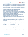
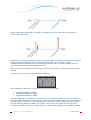
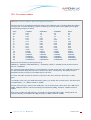
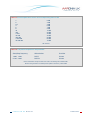
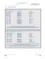
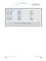
Contents
CHAPTER
PAGE
1.0
Safety Precautions
5
2.0
Scope of Delivery
6
3.0
LC Display
7
4.0
Key Layout
8
5.0
5.1
5.2
5.3
5.4
5.5
5.6
Your first measurements / modes
Operation mode spectrum analysis
The HOLD function
The panning approach
Operation mode exposure limit calculation
Operation mode audio output (demodulation)
Operation mode broadband detector (RF power-detector)
9
10
11
11
12
13
14
6.0
Setting a custom frequency range
16
7.0
7.1
7.2
7.3
7.4
7.5
7.6
7.7
7.8
7.9
7.10
7.11
7.12
7.13
7.14
7.15
7.16
7.17
7.18
7.19
7.20
7.21
7.22
The main menu
Centre (centre frequency)
Span (frequency range width)
fLow & fHigh (Start & Stop frequency)
RBW (bandwidth)
VBW (video filter)
SpTime (sample time)
Reflev (reference level)
Range (dynamics)
Atten (attenuator)
Demod (demodulator / audio analysis)
Pulse (measurement of pulsed signals)
Disp (activate HOLD mode)
Unit (set physical unit: dBm, V/m, mA/m, dBìV)
MrkCnt (set number of markers)
MrkLvl (set starting level of markers)
MrkDis (set marker position)
AntTyp (setup antenna)
Cable (setup cable)
Bright (set display brightness)
Logger (start data logger)
RunPrg (execute program)
Setup (configuration)
18
18
19
19
20
20
20
21
21
21
22
22
23
23
24
24
24
24
25
25
25
26
26
8.0
8.1
8.2
8.3
8.4
8.5
8.6
Correct measurement
Noise floor
Aliases and mirror frequencies
Measuring WLan and cell phones
Sensitivity
Measurement inaccuracy
Cursor and zoom functions
27
27
27
28
28
29
29
9.0
Tips & tricks
30
10.0
10.1
10.2
10.3
Exposure limits
Limits for personal safety
Device limits
Architecture-biological limits
32
32
33
33
SPECTRAN
HF MANUAL
PAGE II of 60
Contents
CHAPTER
PAGE
11.0
11.1
11.2
11.3
Antenna mounting and handling
Single-hand usage with the SMA rod antenna
Two-hands usage with the HyperLOG antenna
Single-hand usage with the HyperLOG antenna
34
34
34
35
12.0
12.1
12.2
12.3
12.4
Connections
External DC input (battery charging)
Audio output
Jog Dial / Volume control
USB connector
37
37
37
38
38
13.0
Hardware setup
39
14.0
Spectrum analysis basics
40
15.0
15.1
15.2
15.3
15.4
15.5
15.6
15.7
15.8
15.9
15.10
RF exposure in practice
Portable phones
GSM & UMTS cellular phones
Cell towers
TV and radio broadcast stations
Satellites
Radio amateurs & CB radio
Bluetooth - the end of all cables
Computers, monitors, cables
Microwave oven
Alarm clocks and radio-controlled clocks
44
44
44
45
46
47
47
47
48
48
48
16.0
What is electrosmog?
49
17.0
17.1
17.2
Physical units
Measuring power [dBm; dBìV]
Field strength [V/m; A/m] and power density [W/m²]
50
50
50
18.0
18.1
18.2
18.3
Formulas for high-frequency
Calculating wave length in [m]
Calculating the close-up range in [m]
Calculating power density [W/m] from power [dBm]
51
51
51
52
19.0
Conversion tables
dBm to W/m² with HyperLOG antenna
53
55
20.0
Frequency tables
Cell phones & GSM900
GSM1800
UMTS
56
56
56
57
21.0
Registration card and warranty
58
22.0
Frequency chart Spectrum Analyser and Antennas
59
SPECTRAN
HF MANUAL
PAGE III of 60
14.0 Spectrum analysis basics
What is a frequency range?
Imagine a giant motorway, several kilometres wide, with thousands of lanes. On this motorway, every
imaginable kind of vehicle can be found: motorcycles, cars, trucks, etc. To not let them get into each
other’s way, every lane is reserved for only a single group of road users: e.g., lane 1 ONLY for cyclists,
lane 3 ONLY for pedestrians, lane 40 ONLY for trucks etc. Depending on the traffic caused by the
individual groups, these lanes also have different widths: For example, the lane reserved for cyclists is far
narrower than that reserved for trucks, etc. High frequency works exactly like this, just that here, the lanes
are the so-called frequency ranges, and the road users are applications (for example, a cell phone, a
microwave oven, a radio-controlled car lock, in effect all appliances that somehow work with radio
waves).
So, every application has its own frequency range for EXCLUSIVE use. By assigning a separate
frequency range for each application, conflicts between different ‘road users’ can be avoided, so that
e.g. a cell phone cannot be disrupted by a microwave oven.
Big differences between exposure limits
Back to our motorway: Of course, all road users also have their own specific speed limits. For our
example, a pedestrian may only walk at up to 4 mph. Cars, however, may speed at up to 70 mph.
Exposure limits for radio applications work similarly: Here, however, the word “speed” is replaced by the
transmitting power: E.g., a broadcast station may have an enormous transmitting power of
1,000,000W or more, in contrast, a radio-controlled car lock only a few mW (1mW = 0,001W) etc. 3
examples of exposure limits in practice:
Frequency range [MHz]
1,880 – 1,900
2,320 – 2,450
5,725 – 5,825
Application
DECT phones
Amateur radio (11cm)
WLan 802.11a
Power limit [W EIRP]
0.25
750
0.025
It is easily visible that each radio application may only use one EXACTLY DEFINED frequency range.
Also, the high differences in admissible transmitting power are noticeable.
Why spectrum analysis?
There are 2 main reasons:
1. You would like to know WHICH radio applications are active
2. You would like to measure the exposure caused by each of the radio applications
separately, e.g. for evaluating exceeding of exposure limits.
Regarding 1):
Let’s reconsider our ‘giant motorway’ example. Remember that every lane was only intended for use by a
single kind of vehicle. Now imagine that a huge bridge crossed this motorway, with you standing on the
bridge and looking down on the motorway. Wow, what a mess!
Now, for example, you would like to know exactly what is happening on the motorway and this for every
single lane. However, the motorway is incredibly wide, so you would need rather good binoculars to be
able to even look a few miles. Let’s just imagine that your binoculars have a range of 4 miles.
Now you would like to know how much traffic there is on a specific lane and how fast it is travelling. So,
you’ll take a piece of paper and write down the number of the lane and the data you evaluated.
SPECTRAN
HF MANUAL
PAGE 40 of 60
Starting at lane 1, you see: nothing! OK, let’s go on with lane 2: nothing either! Now lane 3: OK, there is
some traffic going at 10 mph. Continuing with lane 4: Nothing! etc. until you have reached the last lane.
What have you accomplished now? You’ve performed an ANALYSIS of the entire range of lanes from 04 miles. Or, in other words: You performed a RANGE ANALYSIS. As you know, to analyse something
means breaking it down into smaller parts which can be evaluated. In this case, the 4 mile wide motorway
was that big “something” and the smaller parts were the individual lanes. The word “range” can now be
replaced by the word “SPECTRUM” and there we are: You have performed a SPECTRUM ANALYSIS!
Who would have thought that you were a Spectrum analyser!
Jokes aside: If you now in addition have a lane plan telling you which lane is assigned to which kind of
vehicle, you can exactly determine what kinds of vehicles have just been travelling.
Spectrum analysis in high frequency technology works exactly like that:
There are “lanes” here as well. Though, these lanes are called frequency ranges. The width of these
frequency ranges is measured in the unit Hz (Hertz). However, as the frequency ranges are mostly
found in high Hz ranges, writing them in plain Hz would require huge numbers. Thus, the unit Hz is often
extended to MHz (1,000,000Hz) and GHz (1,000,000,000Hz). Like this, the whole thing becomes much
clearer. So, 1,000,000,000Hz can also be written as 1,000MHz or 1GHz.
But let’s go on. The different kinds of vehicles are called radio applications and have their own
abbreviations: e.g. the radio application “UMTS” (the digital mobile communications standard) has its
own frequency range which spans 1,900 to 2,170MHz (1.9-2.17GHz).
The speed at which the vehicles are travelling can now be replaced by a new expression: the signal
strength or level.
So far, we have now explained the used expressions and units. Now, high-frequency analysis works just
as our motorway example: Our measurement device should evaluate all frequency ranges from 1MHz to
6,000MHz (in pictures, our 6,000m wide motorway). Step by step, every frequency range is evaluated
precisely. First, 0 to 1MHz, then 1MHz to 2MHz etc, up to 6,000MHz. Also, the signal strength of every
frequency range is stored. Like this, we also learn what signal strength was present on which
frequency range.
Real-world examples:
Let’s assume that we want to exactly evaluate the frequency range from 1GHz to 6GHz, and that the
following 3 radio applications were active simultaneously with various signal strengths (in practice,
though, it will mostly be A LOT MORE different applications!):
Frequency range [MHz]
1.880 - 1.900
2.320 - 2450
5.725 - 5.825
Application
DECT portable phone
Amateur radio (11cm)
WLan 802.11a
Reading
40
20
80
How can this be visually displayed on a measurement device? Well, first, we will map the frequency
range from 1GHz to 6GHz on a line from left to right (X-axis):
1GHz ----------------------------------- 6GHz
Ok, this was still pretty simple. Now, we tag each of the 3 applications depending on their frequency on
the right spot of the X-axis and can thus see where they can be found:
SPECTRAN
HF MANUAL
PAGE 41 of 60
Well, this was again pretty simple. And finally, we display the strength of each of the 3 readings as
vertical bars on the Y-axis:
Additionally, we have also adapted the width of each vertical bar to the width of the respective frequency
range of each radio application (the so-called bandwidth): DECT only has 20MHz (1.8801.990MHz=20MHz) of bandwidth, a very small range. Amateur radio, in contrast, already uses a far
higher bandwidth (2.320-2.450=130MHz) and so on.
Well, this wasn’t all that difficult, was it? We can now see ALL information concerning these three signal
sources.
In practice, this will look similar on the SPECTRAN display:
In this example, we also have 3 main signal sources (from left to right):
§
§
§
Signal#1=942MHz at -63dBm
Signal#2=2.024MHz at -23dBm
Signal#3=5.823MHz at -42dBm
These are displayed as vertical bars. The same rule as in our example applies here, too: The higher the
measured signal strength, the higher the bar. Further information regarding each of the bars is displayed
from left to right as markers in the upper display area. On the left, marker 1 is displayed: (the first bar
from the left) with 942MHz at -63dBm. In the middle, marker 2 (the second bar from the left) shows
2,024MHz at -23dBm. On the right, marker 3 (the last, rightmost bar) is displayed: 5,823MHz at -42dBm.
SPECTRAN
HF MANUAL
PAGE 42 of 60
So, what kinds of information have we acquired now?
1. In the entire frequency range from 0-6GHz, there are 3 main signal sources.
2. The frequency and signal strength of all 3 sources is exactly known. So, we have acquired a
quick overview of WHAT is active in this frequency range.
As the exact frequency of the signal sources is now known, it is easy to determine the exact
applications emitting these signals (see also our frequency tables on pages 53-54).
On the basis of these frequency tables, we can determine for e.g. 942MHz: 939.7 to 947.1MHz =
GSM 900 (DL) O2 meaning that this is a GSM900 cell tower (DL=Downlink) of the provider
O2.
SPECTRAN
HF MANUAL
PAGE 43 of 60
15.0 RF exposure in practice
In the real world, you will find hundreds of different high-frequency radiation sources. In the following
pages, we have collected the “most popular” ones, explaining a few peculiarities about each of them. We
will be especially precise with cell towers and cell phones, as that is the field where we receive the largest
amount of inquiries:
15.1 Portable phones (DECT)
Portable phones are replacing more and more regular permanently installed phones in the home and
office. The most important available standard concerning this communications technology is Degitally
Enhanced Cordless Telephone or DECT
DECT
Radio transmission is done digitally and pulsed (at approx. 100Hz, which is audible with
SPECTRAN with activated demodulation), even when no call is being placed, as the base
station of a DECT phone always transmits with full power. The DECT phone, in contrast,
ONLY transmits during a call and also only when the user is actively talking. The transmitting
power is approx. 250 mW at frequencies between 1,880 and 1,900MHz.
15.2 GSM and UMTS cellular phones
So-called “cell phones” are getting more and more popular and already
surpassed the number of conventional telephone network subscribers in 2005.
With cell phones, radio transmission is digital and mostly “pulsed”. UMTS,
however, is “not pulsed”. The transmitting frequencies are, depending on the
network, between 876MHz and 2.2GHz.
You should observe that cell phones steadily increase or decrease their
transmitting power depending on reception quality. This means: The further
away you are from the next cell tower when placing calls, the higher the
exposure to radiation from the cell phone.
If you place calls with a cell phone from your car, you will receive a yet
significantly higher exposure to radiation as the “metal cage” of your car
restricts reception quality (it will mostly switch to full power) and additionally,
the radiation is being reflected in large amounts.
To avoid exposure to this strong radiation, you should use an external antenna for your car. Exposure
then becomes minimal and reception quality will also be significantly better.
Likewise, your cell phone will also transmit with full power inside buildings due to their strong absorption
characteristics.
When you are not placing a call your cell phone also stops radiating. Likewise, when you stop
talking during a call, the cell phone turns down the transmitter power. When the cell phone is turned
on, it will just signal its presence to the network once every 1 to 6 hours, using a short transmission
impulse. Otherwise, it is completely “dead”.
In contrast, if you move around with a cell phone, it will (depending on movement speed and network
availability) repeatedly emit short pulses to login or logout to the respective cell towers.
SPECTRAN
HF MANUAL
PAGE 44 of 60
15.3 Cell towers
Cell towers can be seen nearly everywhere these days. There are only a
few places (like large woodlands) which are still “radiation free”.
The most obvious installations are up to 100m high cell towers (base
stations). In case of only a few customers needing service, these base
stations consist of so-called omnidirectional antennas (mostly one
transmitting antenna in the middle and two reception antennas at either
side).
Omnidirectional base station
with a single cell
Sector-base station with 3
radio cells. Each cell serves
a 120 degree sector
Layout of the base station
shown above
SPECTRAN
Here, the radiation spreads almost equally in all directions. Most base
stations however can provide service to a much larger amount of
customers. In these cases, a group of antennas (so-called radio cells) is
installed on radio towers which only then provide service for a certain
direction (so called sector). Here, when doing measurements, you will
measure different amounts of radiation depending on the position of the
antenna group (see also the radiation pattern on the left). Using this
antenna technology, a significantly higher transmitting power is possible,
using the same amount of space and the same licensing class. In most
cases, you will find the version with three radio cells (triangular installation
with 3 sectors spanning 120 degrees each, see image). Here, you will find a
transmitting antenna on every side, with two similar reception antennas on
either side of the transmitting antenna.
Construction of these “antennas” is very different from that used for
“regular” rod antennas (see picture). They rather resemble some kind of
“fence post”.
All radio cells together make up a huge transmitter network available all
over the country, always appearing as a single, always optimally working
radio cell to the user. In practice, this works as follows: Say you are walking
through a pedestrian area, placing a call with your cell phone. Your phone
will automatically recognize which cell is closest and yields the best
reception, and constantly “jump” automatically to that with the best
reception quality, such that you will always have an optimal, drop-out-free
reception. This whole procedure happens unnoticeable for the user.
HF MANUAL
PAGE 45 of 60
The range of these radio cells (also called “radius”) is highly variable. In
good geographic conditions and with small amounts of users, the radius of
such cells can span several miles. So, in rural areas, you might travel
several miles until the phone changes cells. That is why in such areas,
there are mostly only a few large base stations. In contrast, if many users
are to be expected and reception quality is decreased, like in cities with
large amounts of buildings, walls etc., and these cells might just have a
radius of 100m. To take this into account, of course, the number of radio
cells in cities must be increased significantly. Thus, in big cities like
London, you will find hundreds of individual radio cells.
As even the capacity and range of these cells is often not sufficient, they
are often subdivided once more into smaller, so-called micro cells.
Radio cell map divided
into base stations,
micro- and pico cells
If these are still not small enough, they are further subdivided into the so
called pico cells. Micro and pico cells are very inconspicuous as they are
mostly mounted without any kind of mast or tower and are also of an
extremely small size by themselves.
Thousands of micro and pico cells can be found in most cities, often on the
walls of buildings, but also inside buildings.
As peoples’ acceptance of mobile communications facilities constantly
decreases, though, they are increasingly being disguised. They are hidden
in billboards, company logos, spires, below roofs etc.
For the new generation of mobile communications (UMTS), the number of
cells will need to be tripled, meaning that hundreds of thousands of new,
well disguised cells will become necessary. These will only be detectable
with high-performance measurement equipment like SPECTRAN.
Very hard to find:
A micro cell on a building
wall, above and below
a billboard
Thus, you should keep checking your personal exposure monthly, even
though you can’t see any new antennas.
15.4 TV and radio broadcast towers
TV and radio broadcast towers are a relic from the “stone age” of
information transmission. They are among the strongest radiation sources
in existence.
The highest transmitting powers are used by TV broadcast stations, which
may employ more than 1000kW! (for comparison: a cell tower can use up to
1,500 watts=1.5kW). Short wave radio stations employ transmitting powers
of up to approx. 600kW. FM radio broadcast, employing approx. 100 kW,
are already “more conservative” in this respect. Recently, these are being
converted to digital standards (DVB-T and T-DAB).
Stone-age technology:
Thousands of these broadcast
towers are in operation.
SPECTRAN
Seeing the enormous transmitting powers involved, it is not surprising that
close to these stations (approx. 100m), even the extremely high official
exposure limits are exceeded.
HF MANUAL
PAGE 46 of 60
15.5 Satellites
Modern and almost
exposure-free: Information
transmission via satellites.
Satellites are gaining an ever-increasing importance for information
transmission nowadays. They orbit the earth at a height of approx. 36,000
km in a geostationary orbit. Even though these satellites employ a “high”
transmitting power in the high GHz range, the radiation exposure on earth is
so extremely low due to the vast distance that you need the well known dish
antennas seen everywhere to focus the radiation like a lens. In contrast to
popular misconceptions, these dish antennas and the corresponding LNB
receivers do not radiate. They are completely passive reception devices.
Thus, satellite technology only causes a very low amount of radiation
exposure. If at all, the receiver may cause radiation as it amplifies and
converts signals for later sending them to the TV. For measuring this
radiation, you additionally need an LF measurement device from the
SPECTRAN series.
15.6 Amateur Radio and CB radio
Radio amateurs are allowed transmitting powers of up to 750W divided into
two license classes. CB radio, however, is limited to a maximum 4W of
transmitting power, even though sometimes, significantly higher transmitting
powers are used by illegally employing power amplifiers.
An amateur radio station.
High RF power of up
to 750W is possible.
15.7 Bluetooth - the end of all cables
Ericsson Bluetooth:
From camera to cell phone
via radio.
The radio transmission system “Bluetooth” certainly will find its way into
almost all technical appliances during the next years. Bluetooth is a new,
very affordable, world-wide standard using approx. 2,4GHz and a high data
transfer rate. Transmission is intended to be extremely resistant to
interference by using “frequency hopping”, and also very secure by using
automatic data encryption.
It will replace both the annoying connection cables used for stereos,
speakers, monitors, printers, PCs etc., as well as enable communication
between up to 8 devices like e.g. UMTS cell phones or portable PCs. Just a
few years ahead, it will be pretty normal that the coffee maker will be able to
“talk” to the washing machine or the drinks vending machine...
Bluetooth module in the
year 2000: Newer developments
are just a tenth in size...
Transmitting power and thus exposure to radiation is extremely low with
Bluetooth devices, as power is limited to just 1mW. However, its range is
also limited to only 10m.
Ericsson Bluetooth
headset: significantly
lower radiation
exposure compared to
cell phones
Though, suitable amplifiers will also be available, extending the range to
several 100m.
SPECTRAN
By the way, U.S. market researchers report more than 1.4 billion
Bluetooth devices sold in 2005 alone.
HF MANUAL
PAGE 47 of 60
15.8 Computers, monitors and accessories
An ever increasing number of employees nowadays use a PC at work.
However, more then one out of two UK households today own a PC. PCs
(not as much the monitors) create large amounts of EMF. Specifically the
CPU and various expansion cards emit high doses of high-frequency
EMF. Also, various PC accessories like monitors, printers, scanners etc.
emit low-frequency EMF through their mains cords. We recommend
replacing these cables and possible power strips with our screened cables
and power strips to avoid EMF. This is a quick and easy task and provides
good protection efficiency.
The radiation load caused
by the mains supply
is often as high as the
high-frequency load
from CPU or insert
cards. Because of this,
computers and auxiliary
equipment should be
operated with screened
cables (see Aaronia
price list and cable brochure).
15.09 Microwave ovens
Microwave Ovens:
Although the appliances
are well shielded by
their steel housing the
residual-radiation emission
can still be detected
by SPECTRAN even at
a large distance.
The “microwave”, loved by almost everyone, actually is just a highfrequency transmitter with extremely high transmitting power. While
authoritative exposure limits for cell phones try to avoid warming up of
tissue in the head, exactly this effect is utilised in a microwave oven. The
electromagnetic waves generated in the oven excite vibrations in the water
molecules. The energy from these vibrations in turn causes warming up of
food, etc. The transmitting power used is so extremely high that food heats
up in a matter of only a few seconds. Microwave ovens use high
frequencies of about 2.45GHZ. A bit higher than UMTS, but one thousand
times as much power. These devices are screened badly against the inside
RF radiation The “radiation leakage” is very easily measurable at large
distances without problems using SPECTRAN.
15.10 Radio-controlled (alarm) clocks
These devices do not emit radio waves themselves, they just receive them.
Radio-controlled clocks
do not emit radio waves
themselves. They only
receive them.
SPECTRAN
HF MANUAL
PAGE 48 of 60
16.0 What is electrosmog?
The word “electrosmog” is an artificial term coined in the 70s. The “smog” part is a compound of the two
English words “smoke” and “fog”. Thus, “smog” is roughly equivalent to “dirt”. Finally, “electrosmog” could
alternatively be described as “electric dirt”.
In contrast to “normal” smog which is, year after year, easily noticeable in the cities with our eyes and
nose, “electrosmog” is not detectable with our sense organs. Thus, we can only measure and evaluate
“electrosmog” using dedicated “electrosmog measurement devices”.
Commonly, electrosmog is divided into two types:
§
§
low-frequency electrosmog (e.g. traction power, mains cables, high-voltage lines etc.)
high-frequency electrosmog (e.g. cellphones, cell towers, satellites, radar, radio and TV
broadcast, CB radio etc.)
With our RF (HF-) SPECTRANs, you can only measure high-frequency electrosmog. For measuring lowfrequency electrosmog, you additionally need one of our LF (NF-) SPECTRAN models.
The electrosmog itself consists of electric and magnetic fields:
Electric fields
These fields result from a voltage between two poles. The nearer these poles are to each other
and the higher the voltage, the stronger the electric fields formed between them. Thus, electric
fields are present even when no current is flowing, meaning that even though your lamp, TV etc.
might be turned off, its electrical field is still present at full power! Every cable (especially those
hidden behind walls) is a potential source. Electric fields can be easily screened using conductive
materials. Thus, you should, if possible, replace ALL cables with our screened versions (see our
website).
Alternating magnetic fields
These fields form when current flows through a conductor. The higher the current and the wider
the conductors are placed to each other, the stronger the magnetic field. The only way to
effectively screen against magnetic fields is the utilization of Aaronia Magno-Shield foil or
panels.
High-frequency fields
As electric and magnetic fields do not form separately anymore at higher frequencies, they are
mostly measured as the sum of both field types, expressed as power flux density (W/m² or V/m).
SPECTRAN
HF MANUAL
PAGE 49 of 60
17.0 Units of measurement
SPECTRAN offers several physical units to choose from. These can be selected at any time in the “Unit”
menu. Possible choices are: dBm, dBμV, V/m and A/m. In “Exposure limit calculation” mode, W/m² is
also available.
17.1 Measuring transmission power [dBm; dBμV]
Measurements of communications equipment often show extremely big differences between levels.
Therefore, it is useful to express signal levels in logarithmic units to avoid “drowning” readings in an
endless number of zeros. Thus, our SPECTRAN HF-2025 e.g. already comes up with a measurement
range of -80dBm to 0dBm. As amplification increases 10 fold once every 10dB, “readings” of 0 to
100,000,000 would need to be displayed! However, these “numeric giants” would be nearly unreadable
and result in steady, drastic changes of the displayed values. So, we use the much easier to handle
logarithmic unit dB:
As logarithms are dimensionless, logarithmic readings are always relative to a certain reference level,
i.e., a relationship between two levels is established. A common reference level that has become a
standard in radio technology is 1mW or 1μV. So, logarithmic level readings are expressed in dB
milliwatts [dBm] or dB microvolts [dBμV].
17.2 Field strength [V/m; A/m] and power density [W/m²]
If you don’t feed signals directly and instead perform measurements using an antenna, you will mostly
want to measure the so-called field strength or power flux density instead of power. In professional
measurement technology, mostly only the “manageable” electric field strength is measured, using the unit
V/m. As with dBm, V/m produces manageable readings without endless rows of zeroes.
In contrast, cheap broadband devices often only provide readings of power density (mostly in μW/m²) to
confuse the customer with allegedly huge changes in “electrosmog” strength. This is just as if you
measured distances on motorways in mm: London to Birmingham = 200,000,000mm! Certainly
“impressive”, but just pure showiness, as it’s just 200km. Manageability and readability is left behind, as
the display constantly changes in huge steps. Of course, SPECTRAN can also display power flux density
in μW/m² or other “Giga-units”. However, in contrast to the aforementioned cheap devices, SPECTRAN
offers a practical Auto range feature in W/m² mode, e.g. instead of displaying an endless number of
zeroes, it just displays the corresponding abbreviation f, p, n, μ or m before the unit.
Power flux density S (also called electromagnetic field or power density) is calculated as follows:
W
] = E[mV ] * H[mA ]
S[m²
If H is unknown, the following formula still allows a calculation of S, assuming 377 Ohms as the so-called
“field resistance” of air:
S[
SPECTRAN
HF MANUAL
W
m²
]=
[ ]
V
E² m
377 Ω
PAGE 50 of 60
18.0 Some high-frequency math
In contrast, if E is not known, calculation of S is still possible as follows:
W
] = H²[mA ] * 377Ω
S[m²
Should you wish to calculate the electric field E, use the following formula:
W
E[mV ] = S[m²
] * 377Ω
The magnetic field H can be calculated as follows:
H[
A
m
]=
[ ]
W
S m²
377Ω
18.1 Calculation of wavelength
Wavelength can be calculated using the formula:
λ=
c
f
Here, c corresponds to the speed of light in [m/s] (rounded to 300,000km/s in our example), f to the
frequency of the radiation in [Hz], and to the wavelength in [m].
300000000 m
s = 0,33m
λ=
900000000Hz
(For 900 MHz, the result is 0,33m)
300000000 m
s = 0,17m
λ=
1800000000Hz
(For 1,8 GHz, the result is 0,17m)
300000000 m
s = 0,15m
λ=
2000000000Hz
(For 2 GHz, the result is 0,15m)
Further information concerning wavelength is contained in table 4 on page 64.
18.2 Calculating the “close-up range” in [m]
If you want to perform a measurement, you need to do this outside the so-called close-up range of the
transmitter. The close-up range depends on the transmitter frequency. According to the aforementioned
formula, the close-up range can be determined quickly. Here, you simply need to multiply the resulting
wavelength by a factor of 10 (there are some sources which only use a factor of 3). The result is the
SPECTRAN
HF MANUAL
PAGE 51 of 60
close-up range, i.e. the minimum distance to the transmitter in which a sensible measurement can be
achieved.
Example: For a “900MHz cell phone”, the wavelength is:
300000000 m
s = 0,33m
λ=
900000000Hz
Hence, the close-up range is 0,33m * 10 = 3,3m.
It is easy to see that measurements taken directly next to the cell phone will definitely result in
WRONG readings!
Notice: Inside the close-up range, E and H fields would need to be measured separately. However,
outside the close-up range, both field types are coupled tightly to each other, so knowing the strength of
one of them will be enough to derive the other.
18.3 Calculating power density [W/m²] from power [dBm]
ONLY if you know the transmitter frequency you can calculate power density [W/m²] from power [dBm].
You also need the antenna gain of the used antenna.
The formula you need looks like this:
S=
 p −G 


10 
10
1000
∗ 4λ∗2π
S represents the power density [W/m²], p is the measured power
[dBm], λ is the wavelength of the transmitter frequency [m] and G
the antenna gain [dBi] (dBd-values can be converted to dBi by
adding 2.15).
You get the dBi antenna gain of the HyperLOG antennas easily by looking at the “antenna.ini”-file used
with our “LCS” PC-Software.
Example:
Pretend you measure -40dBm at 950MHz with a HyperLOG 7025 antenna (this antenna offers 4,9dBi at
950MHz). The result is:
S=
 −40 − 4.9 
10 10 
1000
4∗π
∗ 0,31579
2 =
0, 00003236
1000
,566
∗ 012,0997
= 0,00000458 W/m² = 4,08μW/m²
Also see the following conversion table!
SPECTRAN
HF MANUAL
PAGE 52 of 60
19.0 Conversion tables
TABLE 0 Conversion dBm to W/m² with HyperLOG antenna
Assuming the use of an idealized HyperLOG antenna with 5dBi gain and an idealized RG316U cable of
1m length and a constant damping of 1dB, the following conversion table can be applied to the signal
sources below (all figures in W/m²):
dBm
+10
+9
+8
+7
+6
+5
+4
+3
+2
+1
0
-10
-20
-30
-40
-50
-60
GSM900
0.45
0.36
0.28
0.23
0.18
0.14
0.11
0.09
0.07
0.06
0.045
0.0045
0.00045
0.000045
0.0000045
0.00000045
0.000000045
GSM1800
1.9
1.5
1.2
0.95
0.76
0.60
0.48
0.38
0.30
0.24
0.019
0.0019
0.00019
0.000019
0.0000019
0.00000019
0.000000019
GSM1800
2.2
1.8
1.4
1.1
0.89
0.70
0.56
0.44
0.35
0.28
0.022
0.0022
0.00022
0.000022
0.0000022
0.00000022
0.000000022
WLan
3.3
2.7
2.1
1.7
1.3
1.06
0.84
0.67
0.53
0.42
0.033
0.0033
0.00033
0.000033
0.0000033
0.00000033
0.000000033
We assume the following centre frequencies (f):
GSM900 (f = 900MHz), GSM1800/DECT (f = 1850MHz), UMTS (f = 2000MHz) and WLan/microwave
ovens (f = 2450MHz).
The conversion table demonstrates a 10-fold reduction of power density with each 10dB step. Likewise,
the 1dB intermediate steps also express a constant ratio each. Consequently, this table provides a
straightforward way to quickly convert dBm figures into W/m².
Of course, this table can also be utilized in conjunction with other antennas, attenuators or cable
types:
For example, when using our 20dB attenuator (option), you would refer to those rows in the table which
are 20dB higher - i.e. -10dBm instead of -30dBm.
Likewise, when using an antenna with 24dBi gain, you would use those values which are 19dB below
(24dBi - 5dBi [because the values are already pre-multiplied by 5dBi]). Example: -43dBm instead of
-24dBm.
When using a cable with 5dB damping, you would use values 4dB higher (5dB - 1dB [because the
values are already pre-multiplied by 1dB]). Example: -24dBm instead of -28dBm.
SPECTRAN
HF MANUAL
PAGE 53 of 60
TABLE 1 Conversion between W/m², μW/cm² and mW/cm²
0.000,001 W/m²
0.000,01 W/m²
0.000,1 W/m²
0.001 W/m²
0.01 W/m²
0.1 W/m²
1 W/m²
0.000,1 μW/cm²
0.001 μW/cm²
0.01 μW/cm²
0.1 μW/cm²
1 μW/cm²
10 μW/cm²
100 μW/cm²
0.000,000,1 mW/cm²
0.000,001 mW/cm²
0.000,01 mW/cm²
0.000,1 mW/cm²
0.001 mW/cm²
0.01 mW/cm²
0.1 mW/cm²
TABLE 2 Conversion between μW/cm², V/m and A/m
0.000,1 μW/cm²
0.001 μW/cm²
0.01 μW/cm²
0.1 μW/cm²
1 μW/cm²
10 μW/cm²
100 μW/cm²
0.019,4 V/m
0.061,4 V/m
0.194 V/m
0.614 V/m
1.94 V/m
6.14 V/m
19.4 V/m
0.000,051,5 A/m
0.000,162 A/m
0.000,515 A/m
0.001,62 A/m
0.005,15 A/m
0.016,2 A/m
0.051,5 A/m
TABLE 3 Conversion between dBm, dBW and W
0 dBm
-10dBm
-20dBm
-30dBm
-40dBm
-50dBm
-60dBm
-70dBm
-30dBW
-40dBW
-50dBW
-60dBW
-70dBW
-80dBW
-90dBW
-100dBW
0.001W
0.000,1W
0.000,01W
0.000,001W
0.000,000,1W
0.000,000,01W
0.000,000,001W
0.000,000,000,1W
1mW
100μW
10μW
1μW
100nW
10nW
1nW
100pW
dBm = DecibelmilliWatts, dBW = DecibelWatts, W = Watts,
mW = MilliWatts, μW=MicoWatts, nW= NanoWatts, pW=PicoWatts
TABLE 4 Frequency, wavelength and frequency band abbreviations
3 Hz – 30 Hz
30 Hz – 300 Hz
300 Hz – 3 kHz
3 kHz – 30 kHz
30 kHz – 300 kHz
300 kHz – 3 MHz
3 MHz – 30 MHz
30 MHz – 300 MHz
300 MHz – 3 GHz
3 GHz – 30 GHz
SPECTRAN
HF MANUAL
100,000 km – 10,000 km
10,000 km – 1,000 km
1,000 km – 100 km
100 km – 10 km
10 km – 1 km
1 km – 100 m
100 m – 10 m
10 m – 1 m
1 m – 10 cm
10 cm – 1 cm
ULF
ELF
VF
VLF
LF
MF
HF
VHF
UHF
SHF
PAGE 54 of 60
TABLE 5 Power amplification factor and corresponding value in dB
1
2
2.5
4
5
8
10
100
1 000
10 000
100 000
1 000 000
10 000 000
0 dB
3 dB
4 dB
6 dB
7 dB
9 dB
10 dB
20 dB
30 dB
40 dB
50 dB
60 dB
70 dB
dB = Decibel
TABLE 6 Cell phone frequencies and providers
Start/Stop frequency
Abbreviation
Provider
1.880 1.900
5.725 5.825
DECT
DECT2
Private
Private
DECT: Base station always transmits even when not handling calls. 250mW EIRP.
DECT2: New generation of cordless phones (“DECT successor”). 25mW EIRP
SPECTRAN
HF MANUAL
PAGE 55 of 60
20.0 Frequency tables
TABLE 7 UK GSM900 frequencies and providers
Start/Stop frequency
876.2 880.0
880.1 885.1
885.1 890.1
890.1 894.7
894.7 902.1
902.1 909.9
909.9 914.9
Abbreviation
GSM-R (UL)
GSM900 (UL)
GSM900 (UL)
GSM900 (UL)
GSM900 (UL)
GSM900 (UL)
GSM900 (UL)
Provider
Network Rail
Vodafone
O2
Vodafone
O2
Vodafone
O2
921.2
925.1
930.1
935.1
939.7
947.1
954.9
GSM-R (DL)
GSM900 (DL)
GSM900 (DL)
GSM900 (DL)
GSM900 (DL)
GSM900 (DL)
GSM900 (DL)
Network Rail
Vodafone
O2
Vodafone
O2
Vodafone
O2
925.0
930.1
935.1
939.7
947.1
954.9
959.9
(UL) = "Uplink" mostly means “portable device” (mobile transmitter which transmits towards the
base station, e.g. cellphones). Pulsed at 217Hz. Power variable between 20mW-2W (Peak)
(DL) = "Downlink" mostly means “base station” (fixed transmitter which transmits towards the portable device, e.g. cell towers).
Pulsed at 217Hz. Control channel pulsed at 1.736Hz. Power variable between 0,5 and 1,500W ERP. Range of up to 32km.
TABLE 8 UK GSM1800 frequencies and providers
Start/Stop frequency
1,710.1 1,715.9
1,715.9 1,721.7
1,721.7 1,751.7
1,751.7 1,781.7
1,781.7 1,785.0
Abbreviation
GSM18K (UL)
GSM18K (UL)
GSM18K (UL)
GSM18K (UL)
GSM18K (UL)
Provider
O2
Vodafone
T-Mobile
Orange
Private Networks
1,805.1
1,810.9
1,816.7
1,846.7
1,876.7
GSM18K (DL)
GSM18K (DL)
GSM18K (DL)
GSM18K (DL)
GSM18K (DL)
O2
Vodafone
T-Mobile
Orange
Private Networks
1,810.9
1,816.7
1,846.7
1,876.7
1,880.0
(UL) = "Uplink" mostly means “portable device” (portable transmitter which transmits towards the base station, e.g. cell phone).
Pulsed at 217Hz. Power variable between 25mW-1W (Peak)
(DL) = "Downlink" mostly means “base station” (fixed transmitter which transmits towards the portable device, e.g. cell tower).
Pulsed at 217Hz. Control channel pulsed at 1.736Hz. Power variable between 0,5 and 1,500W ERP. Range of up to 32 km.
Private networks operate at much lower powers and are intended for use within confined buildings
SPECTRAN
HF MANUAL
PAGE 56 of 60
TABLE 9 UK UMTS frequencies and providers
Start/Stop frequency
1,920.3 1,934.9
1,934.9 1,944.9
1,944.9 1,959.7
1,959.7 1,969.7
1,969.7 1,979.7
Abbreviation
UMTS (UL)
UMTS (UL)
UMTS (UL)
UMTS (UL)
UMTS (UL)
Provider
Three
O2
Vodafone
T-Mobile
Orange
2,110.3
2,124.9
2,134.9
2,149.7
2,159.7
UMTS (DL)
UMTS (DL)
UMTS (DL)
UMTS (DL)
UMTS (DL)
Three
O2
Vodafone
T-Mobile
Orange
2,124.9
2,134.9
2,149.7
2,159.7
2,169.7
(UL) = "Uplink" mostly means “portable device” (portable transmitter which transmits towards the base station, e.g. cell phone).
Pulsed at 217Hz. Power variable between 25mW-1W (Peak)
(DL) = "Downlink" mostly means “base station” (fixed transmitter which transmits towards the portable device, e.g. cell tower).
Pulsed at 217Hz. Control channel pulsed at 1.736Hz. Power variable between 0,5 and 1,500W ERP. Range of up to 32 km.
SPECTRAN
HF MANUAL
PAGE 57 of 60
21.0 Registration card and warranty
The registration card
AARONIA products are constantly being improved.
As we offer you our replacement and upgrade service* for all of our future measurement devices, we
kindly ask you to send us the included, stamped registration card immediately. Only registered customers
can make use of this service, and only registered clients receive a 10 year warranty on their
measurement device!
* See “The AARONIA warranty”
The AARONIA warranty
Replacement guarantee to “bigger” models
You can exchange your measurement device against a higher-grade model of the same series at any
time by simply paying the price difference. For example, if you have purchased a SPECTRAN HF-2025E
and notice that you need a higher sensitivity after some time, you could replace it with the
SPECTRAN HF-4060 by just paying the difference to this model.
However, for taking advantage of this service, you need to be a registered customer! Thus, you should
complete the included registration card and send it to Aaronia.
Replacement guarantee to newly developed models
As soon as we present new products, you can replace your model with a new Aaronia
measurement device of your choice at any time. This has been realized for the first time in the
year 2000, when we introduced the new Multidetector II series. Customers which sent back their
Multidetector 1 only had to pay half the price for the new Multidetector II series device. The used,
returned units have subsequently been disposed of ecologically friendly by Aaronia.
10 year warranty on all models
We offer 10 years warranty on our measurement equipment. We immediately replace defective units,
without further questions.
SPECTRAN
HF MANUAL
PAGE 58 of 60
22.0 Analyzer & Antenna Frequency chart
Frequency chart SPECTRAN
Spectrum Analyzer
SPECTRAN
HF MANUAL
Frequency chart HyperLOG and BicoLOG
Antennas and Probes
PAGE 59 of 60
© Aaronia Limited
Enterprise House, Unit F4,
Trentham Business Quarter,
Bellringer Road,
Trentham Lakes South,
Stoke-On-Trent
ST4 8GB
t: +44 (0)845 437 9092
f: +44 (0)870 870 0001
www.aaronia.co.uk
SPECTRAN
HF MANUAL
PAGE IV of 60