Download Depth First Search (DFS) And Edge Classification

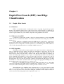
Chapter 3
Depth First Search (DFS) And Edge
Classification
3.1
Depth – First Search
3.1.1 Definition
DFS is a systematic method of visiting the vertices of a graph. Its general step requires
that if we are currently visiting vertex u, then we next visit a vertex adjacent to u which has not
yet been visited. If no such vertex exists then we return to the vertex visited just before u and the
search is repeated until every vertex in that component of the graph has been visited.
3.1.2 Differences from BFS
1. DFS uses a strategy that searches “deeper” in the graph whenever possible, unlikeBFS
which discovers all vertices at distance k from the source before discovering any vertices at
distance k+1.
2. The predecessor subgraph produced by DFS may be composed of several trees,
because the search may be repeated from several sources. This predecessor subgraph forms a
depth-first forest E composed of several depth-first trees and the edges in E are called tree
edges. On the other hand the predecessor subgraph of BFS forms a tree.
3.1.3 DFS Algorithm
The DFS procedure takes as input a graph G, and outputs its predecessor subgraph in the
form of a depth-first forest. In addition, it assigns two timestamps to each vertex: discovery and
finishing time. The algorithm initializes each vertex to “white” to indicate that they are not
discovered yet. It also sets each vertex’s parent to null. The procedure begins by selecting one
vertex u from the graph, setting its color to “grey” to indicate that the vertex is now discovered
(but not finished) and assigning to it discovery time 0. For each vertex v that belongs to the set
Adj[u], and is still marked as “white”, DFS-Visit is called recursively, assigning to each vertex
the appropriate discovery time d[v] (the time variable is incremented at each step). If no white
descendant of v exists, then v becomes black and is assigned the appropriate finishing time, and
the algorithm returns to the exploration of v’s ancestor (v).
If all of u’s descendants are black, u becomes black and if there are no other white
vertices in the graph, the algorithm reaches a finishing state, otherwise a new “source” vertex is
selected, from the remaining white vertices, and the procedure continues as before.
The initialization part of DFS has time complexity (n), as every vertex must be visited
once so as to mark it as “white”. The main (recursive) part of the algorithm has time complexity
(m), as every edge must be crossed (twice) during the examination of the adjacent vertices of
every vertex. In total, the algorithm’s time complexity is (m + n).
1
Algorithm 3.1 DFS(G)
Input : Graph G(V,E)
Output : Predecessor subgraph (depth-first forest) of G
DFS(G)
// initialization
for each vertex u V[G] do
color[u]
WHITE
[u]
null
0
time
for each vertex u V[G] do
if color[u] = WHITE
then DFS-Visit(u)
DFS-Visit(u)
color[u]
GREY
// white vertex u has just been discovered
d[u]
time
time
time + 1
for each v Adj[u] do // explore edge (u,v)
if color[v] = WHITE
then [v]
u
DFS-Visit(v)
color[u]
BLACK // u is finished
f[u]
time
time
time + 1
3.1.4 Properties
1. The structure of the resulting depth-first trees, maps directly the structure of the recursive
calls of DFS-Visit, as u = (v) if and only if DFS-Visit was called during a search of u’s
adjacency list. As a result, the predecessor subgraph constructed with DFS forms a forest of trees.
2. Parenthesis structure: if the discovery time of a vertex v is represented with a left
parenthesis “(v”, and finishing time is represented with a right parenthesis “v)”, then the history
of discoveries and finishes forms an expression in which the parentheses are properly nested.
Theorem 3.1 (Parenthesis Theorem)
In any Depth-First search of a (directed or undirected) graph G = (V,E), for any two
vertices u and v, exactly one of the following three conditions holds :
The intervals [d[u], f[u]] and [d[v], f[v]] are entirely disjoint
The interval [d[u], f[u]] is contained entirely within the interval [d[v], f[v]], and u is a
descendant of v in the depth-first tree, or
The interval [d[v], f[v]] is contained entirely within the interval [d[u], f[u]], and v is a
descendant of u in the depth-first tree
Proof. We begin with the case in which d[u] < d[v]. There two subcases to consider, according to
whether d[v] < f[u] or not. In the first subcase, d[v] < f[u], so v was discovered while u was still
2
grey. This implies that v is a descendant of u. Moreover, since v was discovered more recently
than u, all of its outgoing edges are explored, and v is finished, before the search returns to and
finishes u. In this case, therefore, the interval [d[v], f[v]] is entirely contained within the interval
[d[u], f[u]]. In the other subcase, f[u] < d[v], and d[u] < f[u], implies that the intervals [d[u], f[u]]
and [d[v], f[v]] are disjoint.
The case in which d[u] < d[u] is similar, with the roles of u and v reverse in the above
argument.
Corollary 3.2 (Nesting of descendants’ intervals)
Vertex v is a proper descendant of vertex u in the depth first forest for a graph G if and
only if d[u] < d[v] < f[v] < f[u]
Proof. Immediate from Theorem 3.1.
Theorem 3.3 (White-Path Theorem)
In a depth-firs forest of a graph G(V,E), vertex v is a descendant of vertex u if and only if
at the time d[u] that the search discovers u, v can be reached from u along a path consisting only
of white vertices. This theorem expresses a characterization of when a vertex is descendant of
another in the depth-first forest.
Proof. Direct: Assume that v is a descendant of u. Let w be any vertex on the path between u and
v in the depth-first tree, so that w is a descendant of u. By Corollary 3.2, d[u] < d[w], and so w is
white at time d[u].
Reverse: Suppose that vertex v is reachable from u along at path of white vertices at time d[u], but
v does not become a descendant of u in the depth-first tree. Without loss of generality, assume
that every other vertex along the path becomes a descendant of u. (Otherwise, let v be the closest
vertex to u along the path that doesn’t become a descendant of u.) Let w be the predecessor of v in
the path, so that w is a descendant of u (w and u may in fact be the same vertex) and, by Corollary
3.2, f[w]
f[u]. Note that v must be discovered after u is discovered, but before w is finished.
Therefore, d[u] < d[v] < f[w]
f[u]. Theorem 3.1 then implies that the interval [d[v], f[v]] is
contained entirely within the interval [d[u], f[u]]. By Corollary 3.2, v must after all be a
descendant of u.
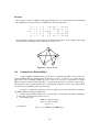
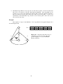
Example
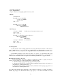
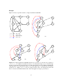
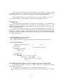
An example of the DFS algorithm is shown in Figure 3.1.
3
U
V
W
Q
X
Y
Z
(a)
1/
1/
(b)
1/
2/
2/5
7/
6/
(h)
1/
2/5
1/
(c)
3/4
1/
(e)
1/
2/
2/5
3/4
1/
2/5
7/8
6/
(i)
1/10
2/5
3/
(d)
3/4
1/
2/5
3/4
6/
(g)
(f)
3/4
2/
3/4
3/4
1/
2/5
7/8
6/
(j)
1/10
2/5
3/4
3/4
11/
7/8
6/9
(k)
1/10
2/5
3/4
7/8
6/9
(l)
1/10
2/5
3/4
11/
7/8
6/9
(n)
12/
7/8
6/9
6/9
(m)
1/10
2/5
3/4
11/
7/8
6/9
(o)
12/
1/10
2/5
3/4
11/
7/8
6/9
(p)
12/13
11/14
7/8
6/9
12/13
(q)
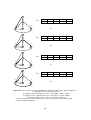
Figure 3.1 : (b) shows the progress of the DSF algorithm for the graph of (a). Starting from node
U we can either discover node V or Y. Suppose that we discover node V, which has a single
outgoing edge to node W. W has no outgoing edges, so this node is finished, and we return to V.
From V there is no other choice, so this node is also finished and we return to U. From node U we
can continue to discover Y and its descendants, and the procedure continues similarly. At stage (l)
we have discovered and finished nodes U, V, W, X, Y. Selecting node Q as a new starting node,
we can discover the remaining nodes (in this case Z).
4
3.2
Edge Classification
During a depth-first search, a vertex can be classified as one of the following types:
1. Tree edges are edges in the depth-first forest G . Edge (u,v) is a tree edge if v was first
discovered by exploring edge (u,v). A tree edge always describes a relation between a node
and one of its direct descendants. This indicates that d[u] < d[v], (u’s discovery time is less
than v’s discovery time), so a tree edge points from a “low” to a “high” node.
2. Back edges are those edges (u,v) connecting a vertex u to an ancestor u in a depth-first tree.
Self-loops are considered to be back edges. Back edges describe descendant-to-ancestor
relations, as they lead from “high” to “low” nodes.
3. Forward edges are those non-tree edges (u,v) connecting a vertex u to a descendant v in a
depth-first tree. Forward edges describe ancestor-to-descendant relations, as they lead from
“low” to “high” nodes.
4. Cross edges are all other edges. They can go between vertices in the same depth-first tree as
long as one vertex is not an ancestor of the other, or they can go between vertices in different
depth-first trees. Cross edges link nodes with no ancestor-descendant relation and point from
“high” to “low” nodes.
The DFS algorithm can be used to classify graph edges by assigning colors to them in a
manner similar to vertex coloring. Each edge (u,v) can be classified by the color of the vertex v
that is reached when the edge is first explored:
white indicates a tree edge
gray indicates a back edge
black indicates a forward or cross edge
3.2.1 Distinguishing between back and cross edges
For every edge (u,v) , that is not a tree edge, that leads from “high” to ”low” we must
determine if v is an ancestor of u: starting from u me must traverse the depth-first tree to visit u’s
ancestors. If v is found then (u,v) is a back edge, else -if we reach the root without having found
v- (u,v) is a cross edge.
Lemma 3.4 A directed graph G is acyclic (DAG1) if and only if a depth-first search of G yields
no back edges.
Proof. Direct: Suppose that there is a back edge (u, v). Then vertex v is an ancestor of vertex u in
the depth-first forest. There is thus a path from v to u in G, and the back edge (u,v) completes a
cycle.
Reverse: Suppose that G contains a cycle c. We show that a depth-first search of G yields a back
edge. Let v be the first vertex to be discovered in c, and let (u,v) be the preceding edge in c. At
time d[v], there is a path of white vertices from v to u. By the white-path theorem, vertex u
becomes a descendant of v in the depth-first forest. Therefore (u,v) is a back edge.
1
See page 7 for definition.
5
Example
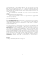
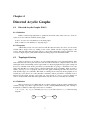
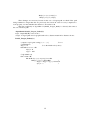
Figure 3.2 shows 3 possible scenarios of edge classification with DFS.
a
b
g
c
d
h
a
b
g
c
h
d
e
f
e
Tree edge
Cross edge
Forward edge
Back edge
f
a
b
g
a
h
c
c
d
f
e
e
(a)
(b)
f
g
h
b
d
(c)
Figure 3.2 : Edge classification with DFS. In the case of scenario (a), the discovery sequence is
a, b, d, e, f, c, g, h. When we reach node d from a, we characterize edge (a.d) as a forward edge
because d is already discovered (from node b). The same applies for node f. When examining the
outgoing edges of e we characterize edge (e,a) as a back edge, since a is already discovered and is
an ancestor of e. Edges (c,d), (c,e) are cross edges because d and e are already discovered and
have no ancestor-descendant relation with c. The same applies for edges (g,b) and (h,d)
6
Chapter 4
Directed Acyclic Graphs
4.1
Directed Acyclic Graphs (DAG)
4.1.1 Definition
DAG is a directed graph where no path starts and ends at the same vertex (i.e. it has no
cycles). It is also called an oriented acyclic graph.
Source: A source is a node that has no incoming edges.
Sink: A sink is a node that has no outgoing edges.
4.1.2 Properties
A DAG has at least one source and one sink. If it has more that one source, we can create
a DAG with a single source, by adding a new vertex, which only has outgoing edges to the
sources, thus becoming the new single (super-) source. The same method can be applied in order
to create a single (super-) sink, which only has incoming edges from the initials sinks.
4.2
Topological Sorting
Suppose we have a set of tasks to do, but certain tasks have to be performed before other
tasks. Only one task can be performed at a time and each task must be completed before the next
task begins. Such a relationship can be represented as a directed graph and topological sorting can
be used to schedule tasks under precedence constraints.We are going to determine if an order
exists such that this set of tasks can be completed under the given constraints. Such an order is
called a topological sort of graph G, where G is the graph containing all tasks, the vertices are
tasks and the edges are constraints. This kind of ordering exists if and only if the graph does not
contain any cycle (that is, no self-contradict constraints). These precedence constraints form a
directed acyclic graph, and any topological sort (also known as a linear extension) defines an
order to do these tasks such that each is performed only after all of its constraints are satisfied.
4.2.1 Definition
The topological sort of a DAG G(V,E) is a linear ordering of all its vertices such that if G
contains an edge (u,v) then u appears before v in the ordering. Mathematically, this ordering is
described by a function t that maps each vertex to a number
{1,2,…,n} : t(v) = i such that t(u) < t(v) < t(w) for the vertices u, v, w of the following
t:V
diagram
u
v
7
w
4.2.2 Algorithm
The following algorithms perform topological sorting of a DAG:
Topological sorting using DFS
1. perform DFS to compute finishing times f[v] for each vertex v
2. as each vertex is finished, insert it to the front of a linked list
3. return the linked list of vertices
Topological sorting using bucket sorting
This algorithm computes a topological sorting of a DAG beginning from a source and
using bucket sorting to arrange the nodes of G by their in-degree (#incoming edges).
The bucket structure is formed by an array of lists of nodes. Each node also maintains
links to the vertices (nodes) to which its outgoing edges lead (the red arrows in Figure 4.1). The
lists are sorted so that all vertices with n incoming edges lay on the list at the n-th position of the
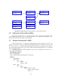
table, as shown in Figure 4.1:
0
v1
1
2
v2
v3
v4
3
Figure 4.1 Bucket Structure Example
The main idea is that at each step we exclude a node which does not depend on any other.
That maps to removing an entry v1 from the 0th index of the bucket structure (which contains the
sources of G) and so reducing by one the in-degree of the entry’s adjacent nodes (which are easily
found by following the “red arrows” from v1) and re-allocating them in the bucket. This means
that node v2 is moved to the list at the 0th index, and thus becoming a source. v3 is moved to the
list at the 1st index, and v4 is moved to the list at the 2nd index. After we subtract the source from
the graph, new sources may appear, because the edges of the source are excluded from the graph,
or there is more than one source in the graph. Thus the algorithm subtracts a source at every step
and inserts it to a list, until no sources (and consequently no nodes) exist. The resulting list
represents the topological sorting of the graph.
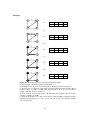
Figure 4.2 displays an example of the algorithm execution sequence.
4.2.3 Time Complexity
DFS takes (m + n) time and the insertion of each of the vertices to the linked list takes
(1) time. Thus topological sorting using DFS takes time (m + n).
4.2.4 Discussion
Three important facts about topological sorting are:
1. Only directed acyclic graphs can have linear extensions, since any directed cycle is an inherent
contradiction to a linear order of tasks. This means that it is impossible to determine a proper
8
schedule for a set of tasks if all of the tasks depend on some “previous” task of the same set in a
cyclic manner.
0
1
0
2
1
2
1
2
2
3
3
4
3
4
3
4
3
4
4
4
(b)
(a)
(c)
(d)
(e)
(f)
Figure 4.2 : Execution sequence of the topological sorting algorithm.
(a)
(b)
(c)
(d)
(e)
(f)
Select source 0.
Source 0 excluded. Resulting sources 1 and 2. Select source 1.
Source 1 excluded. No new sources. Select source 2.
Source 2 excluded. Resulting sources 3 and 4. Select source 3.
Source 3 excluded. No new sources. Select source 4.
Topological Sorting of the graph.
2. Every DAG can be topologically sorted, so there must always be at least one schedule for any
reasonable precedence constraints among jobs.
3. DAGs typically allow many such schedules, especially when there are few constraints.
Consider n jobs without any constraints. Any of the n! permutations of the jobs constitutes a valid
linear extension. That is if there are no dependencies among tasks so that we can perform them in
any order, then any selection is “legal”.
9
Example
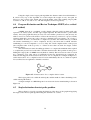
Figure 4.3 shows the possible topological sorting results for three different DAGs.
0
1
0
2
0
1
2
3
1
2
3
3
4
4
0, 1, 2, 3, 4
0, 1, 2, 4, 3
0, 2, 1, 3, 4
0, 2, 1, 4, 3
5
5
4
0, 1, 3, 2, 4, 5
0, 1, 3, 2, 5, 4
0, 1, 2, 3, 4, 5
0, 1, 2, 3, 5, 4
0, 1, 2, 4, 3, 5
0, 1, 2, 4, 5, 3
0, 1, 2, 5, 3, 4
0, 1, 2, 5, 4, 3
6
0, 1, 2, 4, 5, 3, 6
0, 1, 2, 5, 3, 4, 6
0, 1, 2, 5, 4, 3, 6
0, 1, 5, 2, 3, 4, 6
0, 1, 5, 2, 4, 3, 6
Figure 4.3 : Possible topological sorting results for three DAGS.
4.3
Single-Source Shortest Path
In the shortest-path problem, we are given a weighted, directed graph G = (V,E), with
R mapping edges to real valued weights. The weight of path p = (v0, v1,
weight function w: E
…, vk) is the sum of the weights of each constituent edges
w( p )
k
i 1
(vi 1 , vi )
We define the shortest-path weight from u to v by
(u, v)
min{w( p) : u
p
v}
if there is a path from u to v
otherwise
A shortest path from vertex u to vertex v is then defined as any path p with weight
w(p) = (u,v).
There are variants of the single-source shortest-paths problem:
3
Single-destination shortest-paths problem
4
Single-pair shortest-path problem
5
All-pairs shortest-paths problem
We can compute a single-source shortest path in a DAG, using the main idea of the
topological sorting using bucket sorting algorithm. Starting from a given node u, we set the
minimum path (u,v) from u to every node v adj (u ) as the weight w(e), e being the edge (u,v),
and we remove u. Then we select one of these nodes as the new source u' and we repeat the same
procedure and for each node z we encounter, we check if (u,u') + w((u',z)) < (u,z) and if it holds
we set (u,z) = (u,u') + w((u',z)).
10
We must point out that graph G cannot contain any cycles (thus it is a DAG), as this
would make it impossible to compute a topological sorting, which is the algorithm’s first step.
Also, the initial node u is converted to a DAG source by omitting all its incoming edges.
The algorithm examines every node and every edge once at most (if there is a forest of
trees, some nodes and some edges will not be visited), thus its complexity is O(m+n).
4.3.1 Relaxation
This algorithm uses the technique of relaxation. For each vertex v
V, we maintain an
attribute D[v], which is an upper bound on the weight of a shortest path from source s to v. We
call D[v] a shortest-path estimate and we initialize the shortest-path estimates and predecessors
during the initialization phase.
The process of relaxing an edge (u,v) consists of testing whether we can improve the
shortest path to v found so far by going through u. If the shortest path can be improved then D[v]
and [u] are updated. A relaxation step may decrease the value of the shortest-path estimate D[u]
and update v’s predecessor field [u]. The relaxation step for edge (vi,u) is performed at the inner
loop of the algorithm body.
Algorithm 4.1 DAGS_Shortest_Paths(G,s)
Input : Graph G(V,E), source-node s
Output : Shortest-paths tree for graph G and node s, distance matrix D for distances from s.
DAGS_Shortest_Paths(G,s)
compute a topological sorting {v0,v1, …,vn}
// v0 = s
// initialization
D[s]
0
// s is the initial node (source)
for each vertex u s do
D[u]
[u]
null
// algorithm body
for i = 0 to n do
for each edge (vi,u) outgoing from vi do
if D[vi] + w(vi,u) < D[u] then
\
D[u]
D[vi] + w[vi,u] - relaxation
[u]
vi
/
4.3.2 Modifying DAGS_Shortest_Paths to compute single-source longest-paths
The previous algorithm can be used to compute single-source longest-paths in DAGs
with some minor changes:
1. We set D[u]
0 instead of D[u]
during the initialization phase
2. We change the relaxation phase to increase the value of the estimate D[u] by converting
line
11
‘if D[vi] + w(vi,u) < D[u]’ to
‘if D[vi] + w(vi,u) > D[u]’
These changes are necessary because in the case of longest-path we check if the path
being examined is longer than the one previously discovered. In order for every comparison to
work properly, we must initialize the distance to all vertices at 0.
The time complexity of algorithm 4.2 (DAGS_Longest_Paths) is obviously the same as
the one of shortest-path.
Algorithm 4.2 DAGS_Longest_Paths(G,s)
Input : Graph G(V,E), source-node s
Output : Longest-paths tree for graph G and node s, distance matrix D for distances from s.
DAGS_Longest_Paths(G,s)
compute a topological sorting {v0,v1, …,vn}
// v0 = s
// initialization
0
// s is the initial node (source)
D[s]
for each vertex u s do
D[u]
0
[u]
null
// algorithm body
for i = 0 to n do
for each edge (vi,u) outgoing from vi do
if D[vi] + w(vi,u) > D[u] then
\
D[u]
D[vi] + w[vi,u] - relaxation
[u]
vi
/
12
Example
A
2
6
B
3
C
1
1
D:
A
0
B
C
D
A
0
B
6
C
2
D
A
0
B
5
C
2
D
3
A
0
B
4
C
2
D
3
A
0
B
4
C
2
D
3
D
(a)
A
2
6
B
3
C
1
1
D:
D
(b)
A
2
6
B
3
C
1
1
D:
D
(c)
A
2
6
B
3
C
1
1
D:
D
(d)
A
2
6
B
3
C
1
1
D:
D
Figure 4.4 : Execution sequence of the
(e)shortest-path algorithm
(a) Initial graph – All shortest paths are initialized to
(b) Starting from node A, we set shortest paths to B and C, 6 and 2 respectively
(c) From node C, we can follow the edges to B and D. The new shortest path to B is 5
because w(AC) + w(CB) < w(AB). The shortest path to D is A C D and its
weight is the sum w(AC) + w(CD) = 3
(d) From node D, we follow the edge to B. The new shortest path to B is 4 because
w(ACD) + w(DB) < w(ACB).
(e) From node B there is no edge we can follow. The algorithm is finished and the
resulting shortest paths are: A
C, A C D and A C D B with weights
4, 2, 3 respectively.
13
Using the single-source longest-path algorithm, the distance matrix D would initialize to
0, and in every step of the algorithm we would compare the weight of every new path we
discover to the content of the matrix and record the higher value. The resulting longest paths
would be A B, A C and A C D with weights 6, 2 and 3 respectively.
4.4 Program Evaluation and Review Technique: PERT (a.k.a. critical
path method)
A PERT network is a weighted, acyclic digraph (directed graph) in which each edge
represents an activity (task), and the edge weight represents the time needed to perform that
activity. An acyclic graph must have (at least) one vertex with no predecessors, and (at least) one
with no successors, and we will call those vertices the start and stop vertices for a project. All the
activities which have arrows into node x must be completed before any activity "out of node x"
can commence. At node x, we will want to compute two job times: the earliest time et(x) at which
all activities terminating at x can be completed, and lt(x), the latest time at which activities
terminating at x can be completed so as not to delay the overall completion time of the project
(the completion time of the stop node, or - if there is more than one sink - the largest of their
completion times).
The main interest in time scheduling problems is to compute the minimum time required
to complete the project based on the time constraints between tasks. This problem is analogous to
finding the longest path of a PERT network (which is a DAG). This is because in order for a task
X to commence, every other task Yi on which the former may depend must be completed. To
make sure this happens, X must wait for the slowest of Yi to complete. For example in Figure 4.5,
task must wait for Y1 to complete because if it starts immediately after Y2, Y1, which is required
for X, will not have enough time to finish its execution.
Y1
5
X
Y2
2
Figure 4.5 : X must wait for Y1 to complete before it starts
The longest path is also called the critical path, and this method of time scheduling is also
called critical path method.
A simple example of a PERT diagram for an electronic device manufacturing is shown in
Figure 4.6.
4.5
Single-destination shortest-paths problem
This problem is solved by reversing the direction of the edges of the graph and applying
the single-source shortest-path algorithm using the destination as a source.
14
1. IC Design
2. IC Programming
3. Prototyping
ma 12.1.1998
ke 14.1.1998
la 17.1.1998
su 18.1.1998
ke 21.1.1998
to 22.1.1998
4. User - Interface
ti 13.1.1998
su 18.1.1998
5. Field Tests
6. Manufacturing
7. QA Lab Tests
su 25.1.1998
ma 26.1.1998
to 29.1.1998
ma 2.2.1998
to 5.2.1998
ma 9.2.1998
8. Package Design
9. User’s Manual
su 25.2.1998
ke 28.2.1998
su 8.2.1998
ma 9.2.1998
Figure 4.6 : PERT diagram for the production of an electronic device.
4.6
Single-pair shortest-paths problem
Find a shortest path from u to v for given vertices u and v. If we solve the single-source
problem with source vertex u, we solve this problem also, as no algorithms are known to solve
this problem faster than the single-source algorithm.
4.7
All-pairs shortest-paths (APSP)
This problem asks us to compute the shortest-path for each possible pair of nodes of a
graph G = (V, E). To solve it we use the Floyd-Warshall algorithm, for each pair of nodes i, j and
for every node k V , it checks if the shortest path between i and j, p(i,j), it has been found so
far, is larger than the sum p(i,k) + p(k,j). If it is, then it sets the shortest path from i to j as the path
from i to k and from k to j.
The time complexity of this algorithm is O(n3), since we have three loops from 1 to n,
each one inside the previous.
Algorithm 4.3 APSP(G)
Input : Graph G(V,E)
Output : Distance matrix D and predecessor matrix
APSP(G)
//Initialization
for i = 1 to n
for j = 1 to n
D[i,j]
[i,j]
null
for k = 1 to n
for i = 1 to n
for j = 1 to n
if D[i,j] > D[i,k] + D[k,j]
D[i,j]
D[i,k] + D[k,j]
[i,j]
k
15
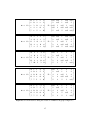
Example
The sequence of steps of APSP for the graph in Figure 4.7 is shown in Figure 4.8. The Distance
(D) and Predecessor ( ) matrices are initialized to the following values
0
8
D
1
0
3
2
0
4
4
7
0
5
0
null
null
1
null null
2
null
null
3
null
null
null
2
3
null
null
4
null
null null
5
null
5
null null
D is the graph’s adjacency matrix with the additional information of the weight of the edges,
while shows the starting node of each edge in respect to D.
2
3
4
8
1
1
7
5
3
-4
2
5
4
Figure 4.7 : Sample Graph.
4.8
Connectivity (Reachability)
Using a slightly modified variation of the Floyd – Warshall algorithm, we can answer the
question whether there is a path that leads from node u to node v, or if node v is reachable from u.
This can be done by running a DFS from node u, and see if v becomes a descendant of u in the
DFS tree. This procedure though takes (m + n) time which may be too long if we want to repeat
this check very often. Another method is by computing the transitive closure of the graph which
can answer the reachability question in O(1) time.
In order to compute the transitive closure of graph G, we can use the Floyd – Warshal
algorithm with the following modifications:
instead of the Distance matrix D we use a Transitive closure matrix T which is initialized
to the values of the Adjacency matrix A of G.
the relaxation part
“if D[i,j] > D[i,k] + D[k,j]
D[i,k] + D[k,j]
D[i,j]
[i,j]
k”
is changed to
“T[i,j]
T[i,j] OR (T[i,k] AND T[k,j])”
16
0
8
K=1
D
1
0
9
3
0
4
K=2
D
K=3
K=4
D
D
5
0
1
8
0
9
D
Figure 4.8 : D and
4
11
3
0
12
4
0
1
null null
2
null
1
null
2
null
3
null
3
null
null
4
null null null
5
null
5
null null
null null
1
null null
2
2
null
1
null
2
5
2
3
null
3
2
6
2
4
null null
5
0
5
null
5
3 6
null
3
1
3
3
2
2
null
1
3
2
4 5
2
3
null
3
2
null null
4
0
0
4
1
8
0
9
11
3
0
12
4
7
10
0
1
1
8
0
9
8
0
0
5
12 4
K=5
2
0
7
7
null null
7
7
5
0
1
1
8
0
7
8
0
0
5
2
null null
0
6
2
4
3
0
5
3
5
3
null
null
4
1
3
4
2
2
null
1
3
2
4 2
4
4
null
3
4
null null
3 3
5
2
0
6
2
4
3
0
5
4
5
3
null
null
4
1
3
4
2
2
null
5
3
2
4 2
4
4
null
3
4
3 3
5
2
12 4 11
0
6
2
4
5
null
2
7
3
0
5
4
5
3
null
7
5
matrices during the execution of APSP for the graph of Figure 4.7.
17
Algorithm 4.4 Transitive_Closure(G)
Input : Graph G(V,E)
Output : Transitive closure matrix T
Transitive_Closure(G)
// initialization
for i = 1 to n do
for j = 1 to n do
T[i,j]
A[i,j]
// A is the adjacency matrix of G
for k = 1 to n do
for i = 1 to n do
for j = 1 to n do
T[i,j]
T[i,j] OR (T[i,k] AND T[k,j])
4.9
Bellman – Ford
The Bellman – Ford algorithm is a single-source shortest-paths algorithm that works for
directed graphs with edges that can have negative weights, but with the restriction that the graph
cannot have any negative-cycles (cycles with negative total weight).
Algorithm 4.5 BellmanFordShortestPath(G,v)
Input : Graph G(V,E)
Output : A distance matrix D or an indication that the graph has a negative cycle
BellmanFordShortestPath(G,v)
// initialization
D[v]
0
for each vertex u v of G do
D[u]
+
for i = 1 to n – 1 do
for each directed edge (u,z) outgoing from u do
// relaxation
if D[u] + w(u,z) < D[z] then
D[z]
D[u] + w(u,z)
if there are no edges left with potential relaxation operations then
return the label D[u] of each vertex u
else
return “G contains a negative weight cycle”
4.9.1
Differences from the Dijkstra algorithm
The Dijkstra algorithm works only with positive weighted graphs with no cycles, while
the Bellman – Ford algorithm works with graphs with positive and negative-weighted
edges and non-negative cycles.
18
The Dijkstra algorithm at every step discovers the shortest path to a new node and inserts
this node to its special set. On the other hand, the Bellman – Ford algorithm uses no
special set, as at every step updates the shortest paths for the nodes that are adjacent to
the node being processed at the current step. Thus, the shortest path to a node is not
determined at an intermediate step, because a new shortest path to this node can be
discovered at a later step.
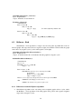
Example
The sequence of steps for the Bellman – Ford algorithm for the graph in Figure 4.9 is
shown in Figure 4.10.
A
D=
A
0
-1
Figure 4.9 : A directed graph with source A
containing a cycle B C D B (with
positive weight w = 1) and its initialized
distance matrix D.
5
B
+
C
+
D
+
E
+
B
3
C
3
-4
2
D
2
E
19
A
5
D=
B
3
3
-4
C
2
D
A
0
B
5
C
3
D
+
E
+
C
1
D
+
E
4
C
1
D
3
E
3
C
1
D
3
E
3
-1
2
(a)
E
A
D=
5
A
0
B
5
B
3
3
-4
C
2
D
-1
2
(b)
E
A
5
D=
B
3
3
-4
C
2
D
A
0
B
5
-1
2
(c)
E
A
D=
5
A
0
B
5
B
3
C
3
-4
2
D
-1
2
(d)
E
Figure 4.10 : The sequence of steps of the Bellman – Form algorithm for the graph of Figure 4.9.
(a) D[B] becomes 5 and D[C] becomes 3.
(b) D[E] becomes 4 and D[C] becomes 1, since D[B] + w(B,C) < D[C].
(c) D[D] becomes 3 and D[E] becomes 3, since D[C] + w(C,E) < D[E].
(d) Nothing changes, since no shortest path can be improved.
At this point there are no more relaxation operations to be performed and the algorithm
returns the distance matrix D.
20