Download III. MSC/PATRAN

III. MSC/PATRAN
III.1 OBJECTIVE
The objective of this manual is to introduce the users to the finite element modeling
capability of MSC/PATRAN and to give hands on, end_to_end guided tour of the software. The
manual shows users how to start MSC/PATRAN, create the geometry model, create the finite
element mesh, define the element and material properties, create load case and the loads and
boundary conditions, prepare data for the analysis, and finally postprocess the results. This
manual does not replace the MSC/PATRAN User's manual (which can currently be browsed
through in the online help menu), but provides sufficient information to start with.
III.2 INTRODUCTION
The finite element method is a proven technique for using computers to model a wide
variety of engineering problems. Its application in the real world was hindered, however, by the
amount of time spent both in producing the raw data to feed a Finite Element Analysis (FEA),
and in interpreting the usually large volumes of results from the analysis. MSC/PATRAN is a
software developed to provide a systematic approach towards making FEA modeling fast and
accurate. It uses a simple step-by-step approach that helps to create, analyze and interpret a
mathematically realistic model of the structure. This approach is built around geometric
modeling, interactive computer graphics, and current finite element theory.
III.2.1 Engineering Functionality
The capabilities of MSC/PATRAN include:
(i)
A full set of tools for the creation of parameterized model geometry. In addition,
MSC/PATRAN has Single Geometric Model (SGM) capability. SGM accesses geometry
data, topology, and evaluators from the CAD (Computer Aided Design/Drafting) system
without transformation and establishes and maintains associativity with the
corresponding MSC/PATRAN finite element entities throughout the entire design and
analysis process.
(ii)
Finite modeling tools for analysis model creation and verification, including mapped
meshing, automatic surface meshing, and automatic tetrahedral solid modeling.
(iii)
A complete set of functional (loads, boundary conditions, and material/element
properties) assignment capabilities, including the capability to assign these directly to the
geometry or the finite element model. In application, this means that the finite element
mesh can be deleted and the geometry remeshed without having to reapply the functional
assignments. All functional assignments can be collected into load cases and named,
modified or deleted at the user's discretion.
(iv)
PATRAN Command Language (PCL) for the customization of MSC/PATRAN, the
performance of variance and design sensitivity studies, and automation of routine,
repetitive tasks.
3.1
III.2.2 Graphical User Interface
The MSC/PATRAN user interface is form driven and truly intuitive, minimizing the time
required to learn the system. At startup, after creating a new database or opening an existing one,
the MSC/PATRAN user interface consists of a control panel, graphics window (view port), and a
command/history window. The control panel controls the parameters for system tasks such as
managing files, setting preferences, manipulating groups and graphics, as well as switching
between interactive applications. The information displayed in the graphics window includes
geometry, finite elements, applied loads, boundary conditions, analysis results and user defined
annotation. The command/history window contains a record of all commands executed during a
MSC/PATRAN session, as well as enabling commands to be entered from the keyboard.
III.2.3 Files
MSC/PATRAN modeling begins with opening a file (new or existing) using the FILE
pick in the upper left corner of the main menu. File management options available under the
FILE pick include: create a new database, open or close an existing database, access CAD
geometry, import IGES models or PATRAN Neutral Files, record and playback session/journal
files.
The MSC/PATRAN relational database defaults to a ”.db” extension and contains a
complete record of user created geometry, finite elements, load cases, load and boundary
conditions, materials, element properties, preferences, and results. MSC/PATRAN database
creation is memory expensive. Each database requires approximately 6MB of disk space.
Therefore old database should be compressed using the Compact Database option under the
FILE pull down menu.
The record of commands shown in the command/history window during a
MSC/PATRAN modeling exercise are stored in editable files that can later be run through
MSC/PATRAN to perform parametric or sensitivity analyses. Two files are created by
MSC/PATRAN to store these commands:
·A session file (.ses extension) which contains the record of all PCL commands for
each interactive session.
·A journal file (.jou extension) which contains a record of all PCL commands for a
particular PATRAN database.
3.2
III.2.4 Analysis Preferences
MSC/PATRAN provides for the user unique analysis preferences i.e. a user can readily
switch between commercial analysis solvers and proprietary in-house codes. Thus the user is not
faced with having to learn the command and syntax of each particular analysis solver. Upon
setting the new preference, MSC/PATRAN automatically updates common element properties,
material properties, loads, boundary conditions, and analysis code forms to those of the newly
selected solver. Note that in this manual, our analysis solver will be MSC/NASTRAN.
III.2.5 Results Visualization
MSC/PATRAN postprocessing is state-of-the-art in its ability to display, sort, combine,
scale, and query in a general way a single results database. After execution, analysis results are
loaded directly into the MSC/PATRAN relational database and can be sorted by time step,
frequency, temperature or spatial location. MSC/PATRAN postprocessing enables the engineer
to filter engineering results by material, element type and property, node and element IDs,
thresholds of results, etc., simultaneously. Display types include but are not limited to: deformed,
fringe, vector, tensor, and engineering X_Y plots. Shear and bending moment diagrams are
available for beam results and a sophisticated text report writer is available to print out all results
in a user defined sorting sequence and format. The insight application within MSC/PATRAN
condenses mountains of raw numerical data into graphical tools and displays for complete,
accurate interpretation of finite element analysis results.
III.2.6 On-Line Help/Documentation
The entire manual of MSC/PATRAN can be browsed through by clicking the left mouse
button on the HELP button of the Top Menu Bar of the Control Panel. All interactive features,
functions, and applications in MSC/PATRAN can be obtained from the completely topical and
context sensitive help on-line. Hypertext links throughout the on-line system allow for instant
retrieval of complex information. The MSC/PATRAN on-line help system eliminates the need
for printed documentation, because the MSC/PATRAN printed documentation is identical to online help files.
III.3 LAB. SESSION 1
III.3.1 Things to know before you start
How to start MSC/PATRAN: After you are in the X-Window environment, just type
'cae-patran2005' at the UNIX prompt.
Hardcopy Printout: You can get a black and white printout through the printer 'cae-yoda'. The
procedures for printing are shown in Section III.3.3. Generally the user prints into a postscript
file. Then the file is sent to a printer of choice by using the 'lpr' command, i.e.
lpr -Pcae-yoda filename
3.3
where 'printer' is the name of the printer and 'filename' is the postscript file generated.
How to quit MSC/PATRAN: To quit MSC/PATRAN, click the left mouse button on the
'File' button of the control panel and select 'Quit' from the pulled down menu. If your want to
start work on another database without quitting P3/PATRAN, you can select 'Save' instead of
'Quit' to save the current database.
Next we will go through the following:
·The menu components of MSC/PATRAN.
·How to use the three-button mouse.
·A highlight of how to modify the view of a model.
·How to print the contents of a viewport.
3.4
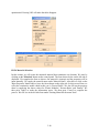
III.3.2 Menu Components of MSC/PATRAN
MSC/PATRAN Control Panel
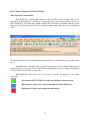
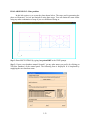
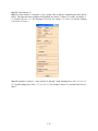
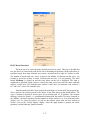
MSC/PATRAN’s Control Panel appears at the top of the screen (example below). The
selections on this panel are divided by a horizontal line. The selection above the line is
MSC/PATRAN’s Top Menu Bar, which includes MSC/PATRAN’s heartbeat and the on-line
help system. The items below the line are a group of radio buttons and a group of Control Panel
icons.
The Menu Bar selections are pull-down menus which will be explained later in using the mouse
(p.3.7)
Radio buttons are mutually exclusive choices in that only one radio button within a group
can be pressed in at one time. They work like the radio buttons in your car. Only one button on
your car radio can be pressed in at one time.
MSC/PATRAN’s heart tells you if it is ready to execute an option or if it is busy
executing.
Green means MSC/PATRAN is ready and waiting to execute a form.
Blue means it is busy, but it can be interrupted with the Hand icon.
Red means it is busy and it cannot be interrupted.
3.5
MSC/PATRAN’s on-line help is an easy to use, hypertext-based documentation system.
You can enter the on-line help either by pressing Help on the Menu Bar, or by placing the cursor
anywhere on a MSC/PATRAN form and pressing the F1 key to get help on that particular form.
If your cursor selects anything that is in magenta in the on-line help, MSC/PATRAN will
quickly “jump” to another page in the on-line help that it is referencing.
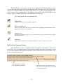
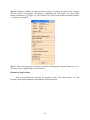
The Control Panel icons are explained below:
Refresh Icon
Redisplays (refreshes) all of the graphics viewports
Display Cleanup Icon
Removes all fringe and marker plots, all automatic titles, highlighting and deformed shape plots.
Repaints the viewport in wireframe mode
Interrupt Icon
Interrupts a command in progress. This is useful when you want to abort out of an executing
MSC/PATRAN form
Undo Icon
Undoes the last executed action of a MSC/PATRAN form when an “Apply” was pressed
MSC/PATRAN Command Window
MSC/PATRAN also has a Command Window that appears at the bottom of the screen
(see below). You can manually enter commands in this window, but mostly this window is used
to view the commands MSC/PATRAN generates when a menu form is executed, and to view
errors or information messages.
The command line. Commands
Can optionally be typed in here.
The history window. You can use the scroll
bars at the bottom and right sides to scroll back
or to scroll to the right.
3.6
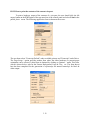
MSC/PATRAN Application Form and Subordinate Form
The radio buttons on the Control Panel will bring up a vertical form on the right side of
the screen. These forms are called the Application forms. There are also smaller forms that are
sometimes displayed which are associated with the specific Application form, and they are called
Subordinate forms.
3.7
III.3.3 Using the Mouse
MSC/PATRAN uses a three-button mouse. Depending on what you are doing, each of the
three buttons will accomplish a specific task in MSC/PATRAN. The following is a summary of
what you will need to know to complete the guided tour.
Using Pull-Down or Option Menus
To use a pull-down or option menu, with the left mouse button, click on menu item. While
holding down the mouse button, drag the mouse to the appropriate selection and then, release the
mouse button.
Selecting From a Listbox
A Listbox has a title at the top and a list of contents. To select an item, use the left mouse button
and highlight the item. To deselect the item, use the left mouse button and highlight the item. To
deselect the item, use the left mouse button and click on the highlighted item.
Overview of the Three Buttons
The left mouse button is used to select model entities. To select more than one entity, hold down
the Shift key while selecting the entities with the left mouse button.
The right mouse button is used to deselect an entity that was selected in error. To deselect more
than one entity, hold down the Shift key while selecting the entities with the right mouse button.
The center mouse button is used to change the view by rotating, translating, or zooming. Keep
the button pressed down and drag the mouse to move the model.
Cursor Selecting Shortcuts
To cursor select model entities with a rectangular box, hold down the left mouse button at the
upper left hand point and drag the cursor to the lower right hand point. Then, release the mouse
button.
To cursor select entities with a polygon shape box, hold down the Control Key (Ctrl) and use the
left mouse button and start picking at arbitrary points A, B, C, D, … to define a closed polygon
box.
3.8
III.3.4 Modifying the View
There are several ways to alter the view of your model, and below are some of the more
common ways.
Using the Middle Mouse Button
As mentioned earlier, you can rotate, translate, or zoom in on your model by dragging the
mouse, while holding down the middle mouse button. To switch the mouse function to rotate,
translate, or zoom, enter View/Mouse Settings…
View/Select Corners…
You can zoom in on a particular part of your model, and at the same time, define a new
viewing center by selecting from the Menu Bar:
3.9
MSC/PATRAN will turn the cursor into a cross-hatch. Define a new “viewport” by
dragging the cursor diagonally and defining a rectangular box:
Drag the cursor along a diagonal direction to select a portion of the model you want to view up
close.
Select View/Fit View… if you want to return the view back to the entire model.
View/Transformations…
You can rotate or translate the view incrementally by selection from the Menu Bar.
A subordinate Transformations form will appear with a matrix of buttons. By pressing any one
of the buttons, you can translate, zoom, or rotate your model incrementally.
For example by pressing a button, MSC/PATRAN will rotate your model about the
screen or model’s Y axis
To perform a “Fit View”, where MSC/PATRAN will resize the view of the model to fit
within the viewport, you would simply press the assigned button.
More view/transformation buttons are shown on the next page.
3.10
Show the entire model with hidden lines
Show the entire model without hidden lines
Show the shaded solid view of the model
Show the end_view in the Y_X plane
Show the end_view in the Z_X plane
Show the end_view in the Z_Y plane
Show the isometric view
Show all the labels (set labels on)
Do not show all the labels (set labels off)
3.11
III.3.5 How to print the contents of the current viewport.
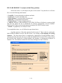
To print a hardcopy output of the contents of a viewport, the user should click the left
mouse button on the 'File' option of the top menu bar of the control panel and select 'Print' in the
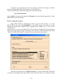
pulled_down menu. The following application form is shown on the screen:
The user then selects ”Postscript Default” under available printers and ”Postscript” under Driver.
The 'Page Setup...' option porvides another form where the either landscape or portrait paper
orientation can be selected. A third form is obtained by clicking on 'Options...' menu. This form,
which is shown below, asks for the Format, Background, Lines & Text, etc. The form shown
here has been completed for the generation of a postscript file named 'manual.ps' for black &
white output.
3.12
To obtain a color postscript file, the 'Color' option is selected for 'Format', the 'White'
option for 'Background' and the 'Actual' option for 'Lines and Text'.
To print the generated postscript file, simply type at the UNIX prompt:
lpr -Pprinter filename
where 'printer' is the name of the printer and 'filename' is the postscript file generated. Use 'caeyoda' for black and white printout.
III.3.6 Creating the Geometry
Each student should go through this section as part of Lab. Session 1. To enter
MSC/PATRAN, just type ”cae-patran2005” at the UNIX prompt. Wait until the system
displays the control panel window and the command history window (see p. 4.4 & 4.5) for
<SC/PATRAN.
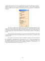
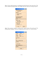
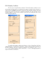
The first step is to create a new database file. This is done by clicking the left mouse button on
”FILE” in the top menu bar of the control panel. This will show a pull down menu from which
”CREATE A NEW DATABASE” is selected. The result is the form shown below:
Note that one should click on “Modify Preference” to check whether MSC/NASTRAN
is selected as the analysis before proceeding. In the form shown above, a new data base name
3.13
“manual” has been entered. The user can supply his/her own name. The OK button is selected
With the left mouse to create a new database named “name.db” ( in this example, manual.db).
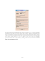
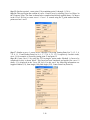
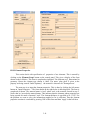
After the database has been created, the following form for model preferences is automatically
displayed:
This form is completed for tolerance limit, approximate maximum dimension of the
model to be created, analysis code of choice and analysis type. The form shown here has been
completed for structural analysis with MSC/NASTRAN as the analysis code. As said earlier (see
p.2), our analysis code will be MSC/NASTRAN. After the form is completed, ”OK” button is
selected.
The next step is to start the creation of a geometrical model. In this lab session, the reader
is taken through creation of basic geometrical entities such as point, curve (1_D), surface (2_D),
and solid (3_D).
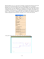
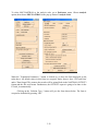
The creation of all geometrical entities is initiated by clicking the left mouse button on
the ”GEOMETRY” radio button of the control panel (see p. 4.4). A typical form that needs to
be completed is shown below (The left mouse button is used to move through the form). Note
that in MSC/PATRAN, the input format of the coordinate of a point, (x, y, z) is given by [x, y, z]
, which is different from that of a vector given by < x, y, z >.
3.14
The above form has been completed for the creation of a point at (x,y,z) = [0,0,0]. It should be
mentioned here that there are several options under ”Action”, ”Object”, and ”Method”. The
choice of combination of options for these three is based on the result desired. Further examples
will be seen in the course of this manual. After a geometrical entity has been created, the figure
shown below (Visible Entities) is seen at the bottom of the screen. This figure highlights
geometrical entities that can be selected by clicking of the left mouse button on the desired
entity. The second point is at [5 0 0].
3.15
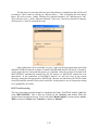
The figure below shows the view port after two points have been created.
The next stage is to create a curve. The form below has been completed for the creation
of a 2_point curve using the two points created earlier:
3.16
The result of applying the above form is shown below:
3.17
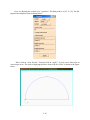
Next, we illustrate the creation of a 3_point arc. The third point is at [2.5, 2.5, 0]. For this
purpose the completed form is shown below:
Don’t click on “Auto Execute.” Instead, click on “Apply”. It gives user a little room to
correct typo errors. The result of applying the above form is the arc (curve 2) shown in the figure
below:
3.18
The next stage is to create a surface. A surface can be created from 2, 3, 4, or N curves
where N is a number to be supplied by the user. An example is given here of how the a surface
can be created from two curves. First, the 3_point arc should be deleted by selecting ”delete”
under ”action” and then clicking on the 3_point arc in the viewport. Next, the following form is
completed for creating a second curve by translating the first 2_point curve:
In the above form, ”<0 5 0>” is entered for the ”Translation Vector”, and ”Curve 1” is
entered for the ”Curve List”. The result of applying this form is shown below:
3.19
After the two curves have been created, the form below is completed for the creation of a
surface:
3.20
Applying the above form, we have the result shown below:
The next stage is to create a solid. Again, there are several ways of creating a solid. In
this example, we are using the 2_surface option. Hence we need to create another surface. This is
done by translating the previous surface 5 units of distance in the z_direction (i.e. Translation
Vector: <0 0 5>). The form completed for surface translation is similar to that of curve
translation with ”Surface” as the ”Object” . After surface translation, we have the result below:
3.21
The rectangular solid is created by completing the form shown below:
Applying the above form, we have the result shown below. To write a note or legend on
the figure, click on “Display,” then “Title” and follow the instructions to fill out the proper
information. Click on “Apply”. In the following picture, the title is given as Solid_Model.
3.22
III.4 LAB SESSION 2: Plate problem
In this lab session, try to create the plate shown below. The steps used in generating the
plate are illustrated. You are not limited to using these steps. You can obtain the same results
using any other combination of steps if you are confident of doing so.
Step 1: Enter MSC/PATRAN by typing 'cae-patran2005' at the UNIX prompt.
Step 2: Create a new database named 'classwk1' (or any other name you prefer) by clicking on
'File/New Database' of the control panel. The following form is displayed. It is completed by
supplying the new data base name.
3.23
Step 3: Set the model parameters by completing the model preferences form shown below. This
form is automatically displayed after a new database has been created or an existing one opened.
Step 4: Start geoemtry creation by clicking on the 'Geometry' button of the radio panel. The
following form is displayed. The form is completed for point 1 (at [x y z] = [0 0 0]) as shown.
3.24
Step 5: Similar to point 1, create points 2 and 3 at [x y z] of [5 0 0] and [0 3 0] respectively.
Step 6: Create point 4 by translation method. This is done by completing the form shown below.
The form has been completed for creation of point 4 by translating point 3 through a vector of <5
0 0>. The Point ID List is shown to be 5 because the 'Apply' button has been clicked on and
point 4 has been created.
Step 7: Similar to point 4, create point 5 by translating point 2 through <0 1 0>.
Step 8: Similar to point 4, create point 6 by translating point 4 through <0.5 0 0>.
Step 9: Similar to point 4, create point 7 by translating point 5 through <0.5 0 0>.
Step 10: Similar to point 4, create point 8 by translating point 7 through <2 0 0>.
Step 11: Similar to point 4, create point 9 by translating point 6 through <2 0 0>.
Step 12: Similar to point 4, create point 10 by translating point 9 through <2.5 0 0>.
Step 13: Similar to point 4, create point 11 by translating point 8 through <2.5 0 0>.
Step 14: Similar to point 4, create point 12 by translating point 10 through <2.5 0 0>.
3.25
Step 15: Similar to point 4, create point 13 by translating point 11 through <2.5 0 0>.
Step 16: This step begins the creation of curves. Create a curve by selecting 'Curve' as 'Object' in
the 'Geometry' form. The form is shown below completed and already applied (hence 2 is shown
in the CUrve ID List) to create curve 1. Curve 1 is created using the 2_point method and the
points used are 1 and 2.
Step 17: Similar to curve 1, create curves 2 through 11 by using 'Starting Point List' 3, 4, 2, 5, 6,
7, 8, 8, 11, 13 and 'Ending Point List' 4, 6, 5, 7, 9, 8, 9, 11, 13, 12 respectively. In other words,
curve 11, for example, is created by joining point 13 and point 12.
Step 18: Create curve 12 by using the '2D ArcAngles' option under 'Method'. A form to be
completed for this is shown below. This form has been completed and applied for curve 12
(hence 13 is displayed in the 'Curve ID List'). For this curve, the following information was
supplied: Radius (1.0), Start Angle (180), End Angle (225), Center Point List (Point 10).
3.26
Step 19: Similar to curve 12, create curves 13 through 15 using the same radius and center point
list as curve 12 but with start angles 225, 270, 315 and end angles 270, 315, 360 degrees.
Step 20: Create curve 16 by using the 'Fillet' option under 'Method'. The region of fillet is shown
in the plate figure. The form displayed to be completed is shown below. This form has been
completed for the fillet curve. The following information was supplied: Fillet Radius (0.5),
Curve/Point 1 List (click on curve 5, then point 5), Curve/Point 2 List (click on curve 4, then
point 5). After the form is completed, P3 asks if the original curves should be trimmed. A
window is displayed for this (see below). The option 'Yes' or ”Yes For All' is selected.
A new point 19 and a new curve 16 are created. The result is shown below:
3.27
Step 21: Trim the curve between points 19 and 5 by using “Edit” under “Action”. Select “Trim”
under “method” and “point” under “option.” Select “Trim” under “method” and “point” under
“option”. Select pont 19 and curve 4 for “Trim Point List” and “Curve/Point List”. Click on
“Apply” after the form is completed.
This step involves merging of two curves 5 and 7. This is done by using the form below. The
new curve formed from the merge is 17. The next two forms contain questions about the
merging. The answer to the first question ( Do you wish to create a dupilicate curve?) is 'No'.
The answer to the second question (Do you wish to delete the original curves?) is 'Yes'.
Follow step 21 to trim the curve between points 5 and 7.
3.28
Step 22: Trim showed 10
Step 23: Create Surface 1 using the 2_curve option. This is done by completing the form shown
below. The form has been completed and applied for surface 1 (hence it is ready for surface 2,
i.e. Surface ID List = 2). The 'Starting Curve List' for surface 1 is 'Curve 16' and the 'Ending
Curve List' is 'Curve 3'.
Step 24: Similar to surface 1, create surfaces 2 through 7 with 'Starting Curve List' 2, 6, 12, 13,
14, 15 and 'Ending Curve List' 1, 17, 8, 9, 10, 11. For example, surface 3 is created from curves 6
and 17.
3.29
Step 25: Before we continue, we want to set the 'Display Property' such that only surface
numbers will be displayed, the curve and point numbers will be hidden. This is done by clicking
on the Display' button of the control panel followed by “Geometry” button. This option allows
the surfaces to be displayed with the fewest number of parametric lines. Next, all label buttons in
the 'Entity Types' section of the form are deactivated except the surface label button. The form is
then applied.
3.30
Step 26: Finally to complete our plate geometry creation, we mirror the figure in the viewport
which is half of our geometry. This done by completing the form below. The mirror plane
normal is defined as {[0 3 0][0 0 0]}. The 'Surface List' is selected to include all existing surfaces
(i.e surfaces 1 through 7).
Step 27: The created geometry can then be printed by following the example shown on p. 4.11.
The user is free to supply his/her own file name.
Homework: Lug Problem
Now as your homework, generate the geometry of the LUG shown below. It is not
necessary for the patch numbers to match those given in the figure.
3.31
III.5 LAB SESSION 3: Analysis of the Plate problem
In this lab session, we will analyze the plate of lab session 2. In particular we will learn
how to use the following radio buttons:
1. Load/BCs: To assign boundary conditions and loads
2. Load Cases: To create and load cases
3. Finite Element: To generate finite element mesh.
4. Materials: To assign material properties.
5. Element Props: To assign element properties.
6. Analysis: Interfaces with NASTRAN via PATNAS (PATran to NAStran) to generate bulk
data file and submit the file to NASTRAN for analysis autoamtically; and via NASPAT
(NAStran to PATran) to read in and translate the analysis (OUTPUT2 format) results.
7. Results: To graphically view analysis results.
To accomplish the above, we will follow the steps shown below.
Load the geometry of the plate generated in lab session 2. This is done by opening the
MSC/PATRAN database saved in the lab session 2 by clicking on File/Opening an existing
database.... The form shown below is completed by supplying the 'Existing Database Name';
indicating the full path to the directory in which the database file is located. If P3 is entered from
the directory that contains the existing database, this database is automatically displayed in
'Database List'. The database can then be selected by clicking on its name in the list.
3.32
III.5.1 Boundary Conditions
The next step is to assign boundary conditions. The desired boundary conditions is to fix
the left edge of the plate, that is, to constrain all six degrees of freedom for the left edge. To
achieve this, the 'Load/BCs' radio button is clicked on. This will bring a display of the form
shown below on the left. This form is completed as indicated. The 'New Set Name' for the
boundary condition is 'fixed'. The new set name is just for the user to identify the data, it is not
used in NASTRAN input file.
To complete the boundary condition specification, we have to 'Input Data' and 'Select
Application Region'. To input data, the 'Input Data...' button is clicked on and the form above on
the right is displayed. This form is completed as indicated. The 'Translations' vector is <T1 T2
T3> = <0 0 0> and the 'Rotations' vector is <R1 R2 R3> = <0 0 0>. This implies that the six
degrees of freedom are constrained.
3.33
To select application region, the 'Select Application Region...' button is clicked on. This
will bring a display of the form shown below. Since we are assigning the boundary conditions
before the finite element mesh is generated, we select 'Geometry' under 'Geometry Filter'. Then
the cursor is moved to 'Select Geometry Entities'. At this point, since we want to apply the
boundary condition to the left edge of the plate, we first click on the edge icon in the 'Visible
Entities' display (see page 4.14). The select menu will then state 'Select a Curve'. At this point,
we cursor select the left edge of the plate by using a rectangular cursor selection. After this is
done, 'Surface 2.1 9.4' (that is, edge 1 of surface 2 and edge 4 of surface 9) is shown in the
'Select Geometry Entities' window. We then click on 'Add' and 'Surface 2.1 9.4' is now shown in
the 'Application Region' window. After this is completed, click on 'OK' to conclude this part.
3.34
Then press 'Apply' on the 'Load/BCs' Application Menu form to conclude the whole step.
At this point, you should have the figure shown below. Notice the 'cones' at the left edge of the
plate at the display lines' point location. These cones represent the three fixed translational and
three fixed rotational boundary conditions. Notice that this boundary condition is applicable to
any future finite element mesh generated for the plate, that is all finite element nodes on the left
edge of the plate will have all six degrees of freedom constrained even though the nodes are yet
to be created.
III.5.2 Applied Loads
The next step is to assign loads to the plate. In this example, we will have two point
(nodal) loads, one in the negative Y_direction and the other in the positive X_direction, the lines
of action of both forces passing through the center of the circular hole in the plate. To achieve
this we complete the same set of forms as for the boundary conditions for each of the point loads,
one after the other, but with the following modifications. The 'Object' is 'Force' rather than
'Displacement'. For the first point load, the 'New Set Name' of '1000_pound_down' can be used
and for the second point load, '10000_pound_right' can be used. These names are just for the
user's benefit, they are not used in NASTRAN's input file. In the 'Input Data...' form, the
following force vectors are provided: <F1 F2 F3> = <0 _1000 0> for the first point load and <F1
F2 F3> = <10000 0 0> for the second point load. For both loads, the moment vector is <M1 M2
M3> = <0 0 0> since no external moment is applied. In the 'Select Application Region...' form,
when the cursor is in the 'Select Geometry Entities' window, the 'Point' icon is selected instead of
the 'Curve' icon. For the first load, cursor select the point at the top of the line dividing surfaces
12 and 13. For the second load, cursor select the point at the middle of the right edge of the plate.
After 'Apply' is pressed for each of the loads in the 'Application Menu' form, the figure below is
the result. Notice the arrows drawn at the selected points signifying the 1000_pound force in the
negative Y_direction and 10000_pound force in the positive X_direction. Each arrow is
displayed as soon as the load corresponding to it is created.
3.35
Now a load case will be created that combines the two point loads and also the specified
boundary conditions. This is done by clicking on the `Load Cases' button of the control panel.
The following form is then displayed. Initially under `Existing Load Cases', we have the
`Default' load case listed. This load case is always present in any analysis, irrespective of how
many more load cases are created by the user. Then we specify the new `Load Case Name' as
`lcase_1'. We make the new load case current. The user is free to give some description for the
new load case under `Description'. This is optional. The next step is to go to the list of `Assigned
Load/BCs Sets' and then select the combinations of loads and boundary conditions that will
constitute the load case being created. For our example, we select all the loads and boundary
conditions in this list to constitute our load case. This means that our load case is made up of
`Displ_fixed_bc', `Force_10000_ibf' and `Force_1000_ibf'. After the form is completed, we
press on `Apply' to conclude the creation of the load case. By now, we should see under
`Existing Load Cases' our newly created load case i.e. `lcase_1'.
3.36
III.5.3 Mesh Generation
The next step is to create the finite element mesh for our plate. This step is divided into
two, the first is to create mesh seeds for the curves bounding our geometry. Mesh seeds allow us
to define exactly how many elements we want on a selected curve or edge of a surface or solid.
The number of mesh seeds on a curve is equal to the number of elements on that curve. An
example is given here of how to create 10 mesh seeds on curve 1 of our geometry. The radio
button 'Elements' is clicked on and the form below on the left is displayed. The form is
completed as indicated. Mesh seeds are created for other curves one after the other such that
surfaces 2 and 9 have 5x10 elements each, surfaces 1 and 8 have 3x4 elements each, surfaces 3
to 7 and 10 to 14 have 4x4 elements each.
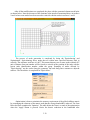
After the mesh seeds have been created, the next thing is to create mesh for our geometry.
This is achieved by selecting mesh as the 'object' in the form shown in the middle below. The
'type' of element is chosen as surface since we are dealing with a 2_D problem. The 'element
topology' selected is 'Quad4', i.e., quadrilateral elements with four nodes. We select 'Isomesh' as
our 'Mesher'. All these selections are then applied to all the surfaces 1 to 14 as indicated in the
'Surface List'. To select all surfaces, we can use the window cursor after we have clicked on
'Surface' icon in the 'Visible Entities' display. After the apply button is pressed, the entire
geometry is subdivided into 'Quad4' elements.
3.37
Before concluding the process of mesh generation, some modifications are made to the
nodes at the interface of surfaces 8 and 9 and also the interface of surfaces 1 and 2. The
modification involves making, at the interface, the nodes for surface 9 coincident with the
corresponding nodes for surface 8 and the nodes for surface 2 coincident with the corresponding
nodes for surface 1. This is achieved by moving the nodes to their new positions. An example is
shown in the form above on the right where 'Node 75' is moved to coincide with 'Node 4'.
3.38
After all the modifications are completed, the plate with the generated element mesh looks
as shown below. Note the skewness of the elements at the interfaces mentioned above in surfaces
2 and 9 where some nodes have been moved to coincide with the nodes in surfaces 1 and 8.
The process of mesh generation is completed by doing the 'Equivalencing' and
'Optimization'. Equivalencing forces nodes that are within some specified tolerance limit to
coincide. The tolerance used here is 0.007. This means that any two or more nodes within 0.007
unit of distance from one another will be forced to coincide at the position of the node with the
lowest node identification number within the group. Examples of nodes affected by
”Equivalencing” are the nodes along the symmetry line and along lines common to adjacent
surfaces. The form below is completed for 'Equivalence'.
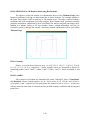
Optimization is done to minimize the memory requirement of the global stiffness matrix
by rearranging the elements of the matrix such that the storage bandwidth is reduced. The form
below has been completed to 'Optimize'. The table below the form is a result of the optimization
when the 'Apply' button is pressed. Notice the drastic reduction in the bandwidth after
3.39
optimization! Pressing 'OK' will make the table disappear.
III.5.4 Material Selection
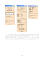
In this section, we will create the structural material that constitutes our elements. We start by
clicking on the 'Materials' button on the control panel. The form shown below on the left side is
displayed. We complete the form as shown. Our material is isotropic and the properties will be
input manually. We supply the material name under 'Material Name'. After this we click on the
'Input Properties' button and we have the form shown on the right side. In this second form, we
select the constitutive model which in this case is 'Linear Elastic'. We also fill out the property
sheet by supplying the shown values for 'Elastic Modulus', 'Poisson Ratio', and 'Density'. We
then press 'Apply' to make the information active. We then press 'Cancel' to complete the
process. We now see in the left side form under 'Existing Materials' the name 'Steel'.
3.40
III.5.5 Element Properties
This section deals with specification of properties of our elements. This is started by
clicking on the 'Element Props' button on the control panel. This gives a display of the form
shown on the left below. This form is completed as indicated. The elements are 2_dimensional in
geometry. Hence the element type chosen is 'shell'. The name `plate_shell' is given to the
property set being created. Under 'Option(s)' the material is chosen to be `Homogeneous'.
The next step is to input the element properties. This is done by clicking the left mouse
button on `Input Properties...'. The form shown on the right below is then displayed. The form is
completed as shown. The material name is 'steel' where steel is the material created in step 5.
Notice that 'm:' precedes the material name. This indicates that the elements whose properties are
being created are made of material `steel'. The element thickness is specified to be `0.125'. For
the problem we want to solve, the information supplied so far is sufficient. Thus the element
properties creation is concluded by pressing `OK' on this form and then `Apply' in the left form.
3.41
“Select Members” box in “Application Region”. (Note that you can not type in the member
numbers directly into “Application Region” box.) One can either type in the members selected
(e.g. Node 1:10, Surface 1:14, …etc.) or use the mouse to select the members by boxing out the
members of concerns. Next, click on “Add” button. The ID numbers of the members selected
will appear in the Application Region” box and then “Apply” in the left form.
III.5.6 NASTRAN Analysis
The next step is to submit our plate to NASTRAN for analysis. It should be mentioned
here that MSC/PATRAN automatically generates the NASTRAN bulk data file (.bdf) and also
submit the .bdf file to NASTRAN. The way we do this is shown here. The first thing is to click
on the `Analysis' button of the control panel. We have the form shown on the left below. We
want to analyze the `Entire Model' in `Full Run'. The `Job Name' we supplied is `classwk1'.
The user is free to use any job name. Notice that the analysis code to be used is
MSC/NASTRAN and the solution type is `Structural'.
3.42
To select MSC/NASTRAN as the analysis code, go to Preference menu. Choose analysis
option, then choose MSC/NASTRAN in the pop-up menu of Analysis Code.
When the `Translation Parameters...' button is clicked on, we have the form displayed on the
right above. All default values in this form are accepted. Notice that we have `OP2 and Print'
under `Data Output' This ensures that results will be printed both in the NASTRAN OUTPUT2
format and the .f06 ascii format. Furthermore, the OUTPUT2 request is going to be done via the
P3 built_in automatically.
Clicking on the `Solution Type...' button will give the form shown below. The form is
accepted as defaulted by pressing “OK”.
3.43
The next step is to create subcases for the analysis. This is done by clicking on `Subcase
Create...' which then displays the form on the left below. To make lcase_1 (i.e. the load case
created earlier) a possible subcase, we click on lcase_1 under `Available Load Cases' and then
press apply. This will place lcase_1 under `Available Subcases'. To make requests for the
variables we want in our output for this subcase, we click on `Output Requests...' and we have
the form on the right below. In this form, we click on `Displacements', `Element Stresses' and
`Constraint Forces' one after the other under `Select Result Type'. Pressing `OK' will place these
three output requests under `Output Requests' as indicated. The indicated output requests will be
printed both in the .f06 and .op2 files. We then press 'Cancel' to conclude this selection. We then
press `Apply' in the form on the left to conclude `Output Requests' and `Cancel' to conclude
`Subcase Create'.
3.44
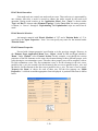
The last step is to select the subcases (out of the subcases created above) that will be used
for analysis. This is done by clicking on `Subcase Select...'. This will display the form shown
below. We click on lcase_1 under `Subcases For Solution Sequence: 101' and then press `OK'.
This will place lcase_1 under `Subcases Selected'. Thus lcase_1 has been selected for analysis.
We then press `Cancel' to conclude this step.
After all these have been concluded, we press `Apply' on the main application menu form
and MSC/PATRAN starts the creation of classwk1.bdf (the bulk data file for the job `classwk1').
At this point, the user waits until this process is completed. After the creation of classwk1.bdf,
MSC/PATRAN automatically submits the file for analysis to NASTRAN without the user
intervention. At the conclusion of NASTRAN analysis, we will now have in the current
directory, among the files generated by NASTRAN, classwk1.op2 (the binary OUTPUT2 format
result file) and also classwk1.f06 (an ascii result file). At this point we are set for post processing
to see graphically our results.
III.5.7 Post Processing
The post processing procedure begins by translating the binary NASTRAN output2 (.op2) file
using 'MSC/PATRAN'. This is done by clicking on the 'Analysis' radio button. When the
required form is displayed (shown below), the option 'Read Output2' is chosen under 'Action',
'Both' is chosen as 'Object' and 'Translate' is chosen as 'Method'.
3.45
Clicking on 'Translation Parameters...' will bring the form shown on the left below. All
settings in this form are accepted as default. Clicking on 'Select Results Files' will bring the
form shown on the right below. The user then supplies the .op2 file in 'Selected Results File'.
This can be done by clicking on the required .op2 file under 'Available Files'. In this example,
we have 'classwk1.op2' under 'Available Files'. We then press 'OK' to accept our selection and
'Cancel' to conclude this step.
3.46
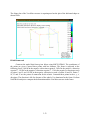
When the translation process is completed, we are ready to view our results. This is
achieved by clicking on the 'Results' radio button on the control panel. We then have the form
shown below on the left in which we have chosen 'Basic' as the 'Form Type'. The result for our
load case, i.e., load_case_1, is automatically placed under 'Select Result Cases'. We then click
on our load case name as shown on the right below and the results that can be displayed by
fringe plotting are indicated under 'Select Fringe Result' while those that can be displayed line
plotting are indicated under 'Select Deformation Result'.
3.47
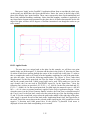
Clicking on '2.1 _ Displacements, Transilational' under 'Select Deformation Result' will lead
to the display of the deformed shape shown below.
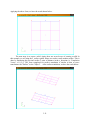
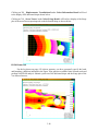
Clicking on '3.1 _ Stress Tensor' under 'Select Fringe Result' will lead to a display of the fringe
plot of the stress tensor superimposed on the deformed shape as shown below.
III.5.8 Homework
For the lug shown on page 4.29 (whose geometry you have generated), specify the loads
and boundary conditions indicated in the figure. Also generate a suitable finite element mesh and
perform NASTRAN analysis. Submit a print out of the deformed shape and the fringe plot of the
Von Misses Stresses.
3.48
III.6 LAB SESSION 4: 1D Beam Problem using Bar Elements
The objective of this lab session is to demonstrate the use of the 'Element Props' radio
button for problems involving one dimensional bar or beam elements. The example problem is
the frame shown below which is made up of 1D straight curves. Geoemtry creation, boundary
conditions and loads assignment, load case creation, finite element mesh generation, material
properties assignment, submission of job to NASTRAN for analysis and post processing can be
handled in a manner similar to the last example. Hence, enough information will only be
provided to guide us through the example. Necessary detailed explanations will be given under
'Element Props'
III.6.1 Geometry
Points 1 to 8 in the above figure are at (x y z) of [0 1 0], [1 1 0], [1 1 1], [0 1 1], [0 0 0],
[1 0 0], [1 0 1], [0 0 1] respectively. 2_Point straight curves are generated as shown by
connecting points 1 and 2, 2 and 3, 3 and 4, 1 and 5, 2 and 6, 3 and 7, 1 and 4, and finally, 4 and
8.
III.6.2 Load/BCs
All six degrees of freedom are constrained for points 5 through 8, that is 'Translations'
and 'Rotations' vectors are both equal to <0 0 0>. Force vectors of <0 _120 50> and <30 40 0>
act at points 1 and 3 respectively. For both points, the moment vector is <0 0 0>. A load case
with any name the user wants is created from the specified boundary conditions and the imposed
point forces.
3.49
III.6.3 Mesh Generation
First mesh seeds are created, one mesh seed per curve. Thus each curve is represented by
one element. After this, a mesh is created to connect the nodes created by the mesh seed
operation. During mesh creation, in the 'Application Menu' form, 'Curve' is chosen under
'Type' and 'Bar2' is chosen under 'Element Topology'. Under 'Curve List', the entire geometry
is chosen, i.e. Curves 1 through 8. 'Equivalencing' and 'Optimization' steps are carried out as
usual.
III.6.4 Material Selection
An isotropic material with 'Elastic Modulus' of 3.E7 and a 'Poission Ratio' of .33 is
specified in the 'Input Properties...' form. You can specify any name for the material under
'Material Name'.
III.6.5 Element Properties
Proceed with element properties' specification as in the previous example. However in
the 'Element Props Application Menu' form, ‘Object’ should be '1D' and 'Type' should be
'Beam'. Under 'Options' select 'General Section' In this example, even though the section
properties of the bar elements are the same, the elements belong to three different groups, each
group having its own orientation vector. Therefore, three property sets will be assigned, each set
for each orientation vector. The first orientation vector is for the elements in the two curves
parallel to the x_axis, the second is for the elements in the two curves parallel to the z_axis, and
the third is for the elements in the four curves parallel to the y_axis. The user is free to supply
'Property Set Name' of choice for each of these sets. For the first property set, 'Input
Properties...' is clicked on and the appropriate form is displayed. A portion of this form is shown
below.
3.50
The information required to be supplied in the above form are listed below. Where a
particular information is applicable to our example, the required value (real scalar or vector) is
given in front of the information. The values given are for the first property set, i.e. for curves
parallel to the x-axis.
Material Name: m:steel (Note: Material name 'steel' is used for illustrative purpose)
Bar Orientation: [1 1 0] (Note: This is the orientation vector, V. See p. 2.25 of the manual).
[Offset @ Node 1]: Not applicable, skip.
[Offset @ Node 2]: Not applicable, skip
[Pinned DOFs @ Node 1]: Not applicable, skip.
[Pinned DOFs @ Node 2]:
Area: 8.0 (Note: This is a real scalar)
[Inertia 1, 1]: 10.667 (Note: See p. 2.16 of the manual).
[Inertia 2, 2]: 2.667
[Inertia 2, 1]: Not applicable, skip.
Torsional Constant: 13.334 (Note: This is 'J'. See p. 2.17 of the manual)
[Shear Stiff, Y]: 0.8333 (Note: See p. 2.17 of the manual).
[Shear Stiff, Z]: 0.8333
[Nonstructural Mass]: Not applicable, skip.
[Y of Point C]: 2. (Note: See p. 2.17 of the manual).
[Z of Point C]: 1.
[Y of Point D]: 2.
[Z of Point D]: _1.
[Y of Point E]: _2.
[Z of Point E]: _1.
[Y of Point F]: _2.
[Z of Point F]: 1.
Station Distances: Not applicable, skip.
For the curves parallel to the y-axis, the vector of 'Bar Orientation' is [1 1 0] while for the
curves parallel to the z-axis, the vector is [0 1 1]. Every other information is the same as for the
curves parallel to the x-axis.
3.51
III.6.6 NASTRAN Analysis
Submit your job for NASTRAN analysis following the steps in III.5.6 of the plate problem. Be
sure to confirm the load cases and boundary conditions before submitting job for analysis.
III.6.7 Post Processing
Perform the post processing of your NASTRAN .op2 result following the steps in Section
III.5.7 of the plate problem. In the 'Result Menu Form' shown below, select 'Von Mises'
(stress quantity to be reported) as the option under 'Result Quantity' and select '6_At Center'
(the position where stress quantity will be reported) under 'Position' at point C which implies
that the stress at Point C defined in Section 6.5 will be reported.
3.52
The fringe plot of the Von Mises stresses is superimposed on the plot of the deformed shape as
shown below.
III.6.8 Homework
Construct the model baja frame given below using MSC/PATRAN. The coordinates of
the points are given. Connect these points with bar elements. The frame is subjected to the
following forces: 100 lbf in the negative z-direction at point 8, 50 lbf in the positive x-direction
at point 17, 120 lbf in the negative z-direction at point 17, 130 in the negative z-direction at each
of points 1 and 2, and 150 lbf in the negative z-direction at each of points 24 and 26. Points 7,
10, 23 and 25 are the points of connection for the wheels. Constrain these points in the x, y, z,
directions. The direction is left free because of the wheels. Use aluminum for the frame. Perform
NASTRAN analysis to compute the deformation and the Von Mises stresses in the frame.
3.53