Download SPAWC: A Scalable Parallel Web Crawler

Computer Science 9868
SPAWC:
A Scalable Parallel Web Crawler
June 02, 2010
Student: Jeffrey Shantz <jshantz(5-1)@csd.uwo.ca>
Instructor: Roberto Solis-Oba
Computer Science 9868
SPAWC: A Scalable Parallel Web Crawler
Jeffrey Shantz <jshantz(5-1)@csd.uwo.ca>
June 02, 2010
Contents
I
SPAWC Overview
1
1 Introduction
1
2 SPAWC Architecture
3
II
2.1
Overview . . . . . . . . . . . . . . . . . . . . . . . . . . . . . . . . . . . . . . . . . .
3
2.2
System Components . . . . . . . . . . . . . . . . . . . . . . . . . . . . . . . . . . . .
3
2.3
Publishing URLs to Crawl . . . . . . . . . . . . . . . . . . . . . . . . . . . . . . . . .
4
2.4
Crawling Process . . . . . . . . . . . . . . . . . . . . . . . . . . . . . . . . . . . . . .
5
2.5
Web Graph Representation . . . . . . . . . . . . . . . . . . . . . . . . . . . . . . . .
7
2.6
System Monitoring and Diagnostics . . . . . . . . . . . . . . . . . . . . . . . . . . . .
8
2.7
Terminating a Crawl . . . . . . . . . . . . . . . . . . . . . . . . . . . . . . . . . . . .
9
2.8
Barriers to Scalability . . . . . . . . . . . . . . . . . . . . . . . . . . . . . . . . . . . 10
2.9
Implementation . . . . . . . . . . . . . . . . . . . . . . . . . . . . . . . . . . . . . . . 11
Dynamic Graph Algorithms
14
3 Background and Terminology
14
4 GraphBench
15
4.1
The Case for Algorithmic Benchmarks . . . . . . . . . . . . . . . . . . . . . . . . . . 15
4.2
Overview . . . . . . . . . . . . . . . . . . . . . . . . . . . . . . . . . . . . . . . . . . 16
4.3
Graph File Format . . . . . . . . . . . . . . . . . . . . . . . . . . . . . . . . . . . . . 18
5 Dynamic All-Pairs Shortest Distance Algorithms
19
5.1
Overview . . . . . . . . . . . . . . . . . . . . . . . . . . . . . . . . . . . . . . . . . . 19
5.2
Naı̈ve Approach . . . . . . . . . . . . . . . . . . . . . . . . . . . . . . . . . . . . . . . 19
5.3
Ausiello et al. . . . . . . . . . . . . . . . . . . . . . . . . . . . . . . . . . . . . . . . . 20
5.4
APSD - Algorithm 1 . . . . . . . . . . . . . . . . . . . . . . . . . . . . . . . . . . . . 21
5.4.1
Asymptotic Analysis . . . . . . . . . . . . . . . . . . . . . . . . . . . . . . . . 23
5.4.2
Correctness . . . . . . . . . . . . . . . . . . . . . . . . . . . . . . . . . . . . . 23
ii
Computer Science 9868
SPAWC: A Scalable Parallel Web Crawler
5.5
Jeffrey Shantz <jshantz(5-1)@csd.uwo.ca>
June 02, 2010
Benchmarks . . . . . . . . . . . . . . . . . . . . . . . . . . . . . . . . . . . . . . . . . 24
6 Dynamic Strongly-Connected Components Algorithms
6.1
6.2
6.3
25
Naı̈ve Approach . . . . . . . . . . . . . . . . . . . . . . . . . . . . . . . . . . . . . . . 25
6.1.1
Asymptotic Analysis . . . . . . . . . . . . . . . . . . . . . . . . . . . . . . . . 26
6.1.2
Correctness . . . . . . . . . . . . . . . . . . . . . . . . . . . . . . . . . . . . . 26
Algorithm 1 . . . . . . . . . . . . . . . . . . . . . . . . . . . . . . . . . . . . . . . . . 27
6.2.1
Asymptotic Analysis . . . . . . . . . . . . . . . . . . . . . . . . . . . . . . . . 29
6.2.2
Correctness . . . . . . . . . . . . . . . . . . . . . . . . . . . . . . . . . . . . . 30
6.2.3
Benchmarks Based on Block Width
. . . . . . . . . . . . . . . . . . . . . . . 31
Benchmarks . . . . . . . . . . . . . . . . . . . . . . . . . . . . . . . . . . . . . . . . . 31
7 Maintaining Statistics for the SPAWC Web Graph
32
III
34
Conclusions
8 Related Work
34
8.1
Web Crawling . . . . . . . . . . . . . . . . . . . . . . . . . . . . . . . . . . . . . . . . 34
8.2
Dynamic Graph Algorithms . . . . . . . . . . . . . . . . . . . . . . . . . . . . . . . . 34
9 Conclusions and Future Work
35
Appendices
36
A SPAWC User Manual
36
A.1 Prerequisites . . . . . . . . . . . . . . . . . . . . . . . . . . . . . . . . . . . . . . . . 36
A.2 Getting Started . . . . . . . . . . . . . . . . . . . . . . . . . . . . . . . . . . . . . . . 36
A.3 Starting a Crawl . . . . . . . . . . . . . . . . . . . . . . . . . . . . . . . . . . . . . . 37
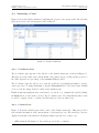
A.4 Monitoring a Crawl . . . . . . . . . . . . . . . . . . . . . . . . . . . . . . . . . . . . . 38
A.4.1 Coordinator Pane
. . . . . . . . . . . . . . . . . . . . . . . . . . . . . . . . . 38
A.4.2 Crawlers Pane . . . . . . . . . . . . . . . . . . . . . . . . . . . . . . . . . . . 38
A.4.3 Statistics Pane . . . . . . . . . . . . . . . . . . . . . . . . . . . . . . . . . . . 39
A.4.4 Degree Distributions Pane . . . . . . . . . . . . . . . . . . . . . . . . . . . . . 39
A.5 Diagnostics . . . . . . . . . . . . . . . . . . . . . . . . . . . . . . . . . . . . . . . . . 40
iii
Computer Science 9868
SPAWC: A Scalable Parallel Web Crawler
B GraphBench User Manual
Jeffrey Shantz <jshantz(5-1)@csd.uwo.ca>
June 02, 2010
41
B.1 Prerequisites and Installation . . . . . . . . . . . . . . . . . . . . . . . . . . . . . . . 41
B.2 Getting Started . . . . . . . . . . . . . . . . . . . . . . . . . . . . . . . . . . . . . . . 41
B.3 Usage Examples . . . . . . . . . . . . . . . . . . . . . . . . . . . . . . . . . . . . . . 41
C Benchmark Graphs
44
C.1 Insertion Sequences Requiring Cubic Updates . . . . . . . . . . . . . . . . . . . . . . 44
D References
46
iv
Computer Science 9868
SPAWC: A Scalable Parallel Web Crawler
Jeffrey Shantz <jshantz(5-1)@csd.uwo.ca>
June 02, 2010
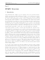
Part I
SPAWC Overview
1
Introduction
As the World Wide Web continues to grow at a rapid pace, the need for an effective means to
distill the vast information available and find pages relevant to one’s needs has never been greater.
Current search engines deploy crawlers or spiders to crawl from page to page on the Web, examining
the contents of and storing information relevant to each page, typically indexed by keywords found
in the page that a crawler determines to be most representative of its contents. A user can then
later search this index by specifying a set of keywords describing the information sought, and pages
matching these keywords are returned, typically ranked in order of relevance to the search terms
specified. Because pages on the Web are frequently added, updated, and removed, it is critical that
search engines ensure the timeliness of their indices. This implies that, at the very least, the most
frequently updated pages must be crawled often to keep search results from becoming stale.
Search engines generally do not strive to index the entire World Wide Web. After all, doing so
would consume far too much time and resources, and the benefit derived from indexing every page
would likely not justify its cost. This is because, while each page on the Web is addressed uniquely
by a Uniform Resource Locator (URL), many pages differ very little from one another, if at all [1].
For instance, consider a fictional calendar located at http://www.cal.zzz/view?m=Jul&y=2010.
While the URL http://www.cal.zzz/view?m=Aug&y=2010 is distinct from the former, it is likely
that their contents will be mostly similar, with identical headers, navigation bars, footers, and other
boilerplate content [1]. As such, search engines strive to index a representative subset of the Web.
Google’s last reported index size before it stopped making such information publicly available in
2005 was over 8 billion pages [2], up from 1 billion pages in 2000, and just 26 million pages in
1998 [1]. However, with Google estimating as of July 2008 that the Web contains over one trillion
unique addresses, visiting even a fraction of the URLs on today’s Web in a timely manner demands
efficient crawling techniques.
One can easily see that sequential downloading will be insufficient for the timely crawling of anything
greater than a tiny subset of the total pages on the Web. To see this, consider an optimal scenario
in which one has a connection speed of 25 Mbps, and assume zero congestion rates, zero processing
time after downloading a page, and no asymmetry in Internet connection speeds. With the average
size of the textual content of a Web page estimated to be approximately 25 KB [3], one could
crawl the Web at a rate of 128 pages per second. At this rate, crawling just one billion pages
(0.1% of Google’s estimate of 1 trillion URLs) would take three months! Furthermore, given the
asymmetry of Internet connection speeds in reality, increasing the speed of one’s connection will
1
Computer Science 9868
SPAWC: A Scalable Parallel Web Crawler
Jeffrey Shantz <jshantz(5-1)@csd.uwo.ca>
June 02, 2010
do little to increase crawl rates. This is because download rates are constrained by the slowest link
in a connection, and thus it is likely that the connection speed of the remote server from which a
page is being downloaded will present a bottleneck, even if one is crawling on an extremely high
speed connection. As such, sequential downloading is insufficient for crawling the Web efficiently.
One alternative to sequential crawling is to run multiple crawlers in parallel, each downloading
distinct pages concurrently. Assuming one has sufficient bandwidth, the rate at which pages are
crawled can be greatly increased simply by spawning additional crawlers, as needed. The Scalable
Parallel Web Crawler (SPAWC) presented in this paper was designed on this concept, offering a
means to efficiently crawl the Web in parallel, and presenting a scalable solution that allows crawl
speeds to be tuned as needed. As will be discussed in section 2.9, using the SPAWC architecture, it
is theoretically possible to crawl thousands of pages per second in parallel, assuming the availability
of a sufficient number of crawler machines in the network, as well as sufficient network bandwidth.
While the focus of this project was not to index the contents of pages crawled, all pages are
downloaded in their entirety to parse the links they contain, and thus indexing could be integrated
into the architecture with relative ease.
Rather than indexing Web pages, SPAWC builds a representation of the crawled Web graph in memory, and statistics such as graph diameter, average node distance, and the distribution of incoming
and outgoing links are computed dynamically as new pages are crawled. Computing statistics for
a dynamically changing graph presents an interesting challenge in comparison to static graph algorithms, as these statistics must be updated as graph edges are inserted or deleted. For reasons
of efficiency, one typically seeks to update statistics only for those vertices that have been affected
by changes in the graph, without having to recompute statistics for the entire graph from scratch.
In addition to presenting the SPAWC architecture, this paper also makes the contribution of providing an overview of several dynamic graph algorithms used by SPAWC in computing statistics,
such as dynamic algorithms for computing all-pairs shortest path distances (APSD), and stronglyconnected components (SCC). In addition, a space-efficient algorithm for dynamically computing
the transitive closure and strongly-connected components of a graph is developed and presented.
The rest of this paper is organized as follows. Part I introduces the SPAWC architecture, detailing
the major components in the system and the manner in which they interact. Part II presents
several dynamic APSD and SCC algorithms, and introduces a benchmarking framework developed
to compare the running time of each algorithm using a variety of sparse and dense graph insertion
sequences. Benchmark data for each algorithm is presented to justify the choice of dynamic graph
algorithms selected for use in SPAWC. Part III presents work related to SPAWC, along with
conclusions and directions for future work. Appendix A presents a user manual for SPAWC, while
Appendix B presents a user manual for the graph algorithm benchmarking framework developed
to test the algorithms presented in this paper. Finally, Appendix C describes the graph insertion
sequences used in benchmarks presented in this paper.
2
Computer Science 9868
SPAWC: A Scalable Parallel Web Crawler
2
2.1
Jeffrey Shantz <jshantz(5-1)@csd.uwo.ca>
June 02, 2010
SPAWC Architecture
Overview
SPAWC is a scalable Web crawler which employs multi-processing to allow multiple crawler processes to run in parallel. While it is possible to run crawlers on multiple threads, such a solution
lacks the scalability desired for the system, since threads can only be spawned on a single machine,
limiting the total number of concurrent crawlers possible. By contrast, SPAWC crawlers are executed as separate processes. These crawler processes consume more resources than they would were
they to be implemented as threads, limiting the total number of crawlers that can run concurrently
on a given system. However, multi-processing offers the distinct advantage of allowing crawler
processes to be distributed amongst numerous machines in the network. As such, scalability is
greatly enhanced, since increasing the rate at which pages are crawled can be achieved by simply
spawning new crawler processes on systems within the network. Furthermore, as the following section will discuss in detail, many of the complexities involved in multithreaded programming – and
even traditional multi-processing – are eliminated in the SPAWC architecture, such as the need to
limit concurrent access to shared memory via mutexes and locks. Instead, the SPAWC architecture
is designed based on a high-performance, producer-consumer model whose simplicity translates to
easier debugging and maintenance.
2.2
System Components
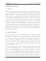
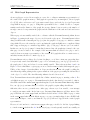
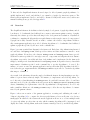
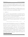
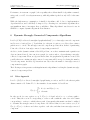
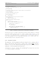
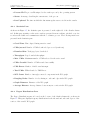
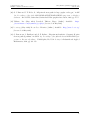
Figure 1 presents the major components of the SPAWC architecture, along with the communication
model employed. In SPAWC, a single coordinator process is executed, with the user specifying
the initial number of crawler processes desired, the maximum number of URLs to crawl, and
one or more seed URLs at which to begin crawling. The coordinator then spawns the specified
number of crawlers, provides instructions to the crawlers on which URLs to crawl, handles new
links returned by the crawlers from pages downloaded, and monitors the status of active crawler
processes. Additionally, the coordinator maintains an internal representation of the Web graph
being crawled, updating the graph dynamically as crawlers return successfully downloaded pages
along with the links they contain.
To simplify communication, the coordinator never directly communicates with a given crawler process. Instead, all communication between the coordinator and crawlers takes place asynchronously
through message queues (MQ) that the coordinator constructs upon initialization. These queues
are provided by a MQ server, which allows messages to be posted to and later retrieved from queues
created on the server. Typically, MQ servers provide very high-throughput, low-latency access to
queue data, while simultaneously hiding the complexities involved in distributed communication.
Using a server-specific API, one need only use methods such as publish to send a message to a
queue, and pop to retrieve the message at the head of the queue. All other details involved in
3
Computer Science 9868
SPAWC: A Scalable Parallel Web Crawler
Jeffrey Shantz <jshantz(5-1)@csd.uwo.ca>
June 02, 2010
Figure 1: SPAWC Architecture
facilitating this process are handled by the MQ server and its corresponding API library.
An administrator can initiate and monitor the progress of a crawl through a Web-based dashboard
developed for SPAWC. The dashboard monitors the status of the coordinator, and also displays
information stored by the coordinator in the system database, describing the current status of each
running crawler process. Additionally, the Web dashboard allows administrators to dynamically
change the number of executing crawler processes, allowing the crawl rate to be tuned, as needed.
2.3
Publishing URLs to Crawl
When an administrator starts a crawl, the dashboard spawns a new coordinator process, providing it
with a list of seed URLs specified by the administrator, as well as the maximum number of URLs to
crawl, and the initial number of crawler processes to use. The coordinator then publishes the set of
seed URLs to the crawl queue, shown in Figure 1. Whenever the coordinator publishes URLs to this
queue, it uses a two step process in which it first places the URLs in a urls to crawl list it stores
locally. It then calls the Publish-URLs algorithm listed in Figure 2 to publish the seed URLs to
the crawl queue. This indirect publication is done to ensure that the number of URLs published to
the crawl queue (published count) never exceeds the maximum number of URLs specified by the
administrator (max urls). Publish-URLs iterates through this list, and while published count
is less than max urls, Publish-URLs removes the next URL from urls to crawl, and publishes
it to the crawl queue, incrementing published count. Later, if a crawler reports that a URL could
not be successfully crawled, the coordinator decrements published count to allow another URL
stored in urls to crawl to be published to the crawl queue. Hence, published count can be
described by the following equation:
published count = |urls crawled| + |crawl queue| − |error urls| ≤ max urls
4
Computer Science 9868
SPAWC: A Scalable Parallel Web Crawler
Jeffrey Shantz <jshantz(5-1)@csd.uwo.ca>
June 02, 2010
Publish-URLs()
1 while ((published count < max urls) & (!urls to crawl.empty()))
2
url = urls to crawl.pop()
3
4
if (! published urls.contains(url))
5
crawl queue.publish(url)
6
published count++
7
published urls[url] = true
Figure 2: Publishing URLs to the crawl queue
Notice that Publish-URLs also checks to ensure that each URL to be published to the crawl queue
has not been previously published. This duplicate detection process ensures that each distinct URL
is crawled at most once, and is performed in O(1) time using a published urls hash. Publishing to
the crawl queue is an operation specific to the MQ server in use, but should also be a constant time
process. As such, in the worst case, Publish-URLs runs in time linear in the size of urls to crawl.
2.4
Crawling Process
When the coordinator is started, it is provided with the initial number of crawler processes desired.
Before publishing the set of seed URLs to the crawl queue, the coordinator spawns the specified
number of crawler processes, providing them with the IP address and port on which the MQ server
is listening. A crawler that is idle continuously polls the crawl queue for a new URL. If none is
currently available, the crawler waits for a configurable interval of time (currently 1 second) and
polls the queue again. Otherwise, the crawler removes the URL at the front of the crawl queue
and proceeds to download the page at the given address. Once the crawl attempt is complete, it
places a Page object describing the attempt in the reply queue. This object contains information
such as whether or not the page was downloaded successfully, and, if so, its total size and a list of
the outbound links it contains.
Since the focus of the project was placed on building a representation of the Web graph, and
not indexing pages and files crawled, SPAWC crawlers currently only process Hypertext Markup
Language (HTML) pages. This limitation is enforced by crawler processes in a two-fold manner.
First, the extension of a URL is examined by the crawler to determine if it matches a common
binary extension, such as .pdf, .jpg, .mp3, or .doc. If so, the crawler will immediately place an
error for the URL in the reply queue, without attempting to download it. Otherwise, the crawler
will attempt to download the file at the URL, and will examine the MIME type [4] reported by
the server, which describes the content type of the file at the requested URL. If the server reports
a MIME type other than text/html – the standard content type indicating that the file requested
is a HTML page – the crawler terminates its connection to the server without downloading the
contents of the file, and similarly places an error for the URL in the reply queue.
5
Computer Science 9868
SPAWC: A Scalable Parallel Web Crawler
Process-Next-Reply(reply queue)
1 page = reply queue.pop()
2
3 if page = = null
4
return
5 elseif (! page.download success)
6
error urls[page.url] = true
7
published count-8
Publish-URLs()
9
return
10
11 page.seqnum = downloaded pages.size
12 downloaded pages[page.url] = page
13
14 foreach url in page.links
15
urls to crawl.insert(url)
16
17 Publish-URLs()
18 Update-Graph(page)
Jeffrey Shantz <jshantz(5-1)@csd.uwo.ca>
June 02, 2010
// Retrieve the next page from the reply queue
// If no page is available, return
// If the page was unsuccessfully crawled
// Store its URL in the error pages hash
// Do not count it as a published page
// Otherwise, give the page a unique integral sequence number
// Store the page indexed by its URL in the downloaded pages hash
// Iterate through each hyperlink in the page
// Add each link to the list of URLs to be published to the crawl queue
Figure 3: Processing the next page in the reply queue
If a URL points to a valid HTML page, the crawler will download the page in its entirety and
proceed to parse the links contained within it. Any relative URLs found are converted to absolute
URLs (e.g. /about.html to http://www.cal.zzz/about.html), and URLs that point to invalid
extensions, as discussed above, are skipped. Finally, duplicate links are removed, and the resulting
list of URLs is inserted into a list of links stored in the Page object describing the crawl attempt,
and this object is published to the reply queue.
A thread running in the coordinator process monitors the reply queue, processing new Page objects
as they become available. When a new reply becomes available, the coordinator executes the
Process-Next-Reply algorithm, shown in Figure 3. This algorithm removes the next Page
object from the reply queue, and checks to see if it represents a successful crawl attempt, as shown
on line 5. If the attempt failed, the URL is stored in the error urls hash, described shortly. As
noted earlier, it then decrements published count and calls Publish-URLs to allow another URL
possibly waiting in the urls to crawl list to be published to the reply queue.
Otherwise, if the crawl attempt was successful, the coordinator assigns a unique integral sequence
number to the Page object, and stores it in the downloaded pages hash for later retrieval. It then
iterates through the list of links found in the page, inserting them into the urls to crawl list, as
shown in lines 14 and 15. Finally, it calls Publish-URLs to publish them to the crawl queue,
and calls Update-Graph(page), described in section 2.5, passing in the Page object to update its
graph representation based on the new page crawled.
In the worst case, the time complexity of Process-Next-Reply is dominated by, and thus equal
to, the asymptotic complexity of Update-Graph, described next.
6
Computer Science 9868
SPAWC: A Scalable Parallel Web Crawler
2.5
Jeffrey Shantz <jshantz(5-1)@csd.uwo.ca>
June 02, 2010
Web Graph Representation
As new replies are received from crawler processes, the coordinator maintains a representation of
the crawled Web graph in memory. This graph is represented by an unweighted, directed graph
G = (V, E), where each vertex v ∈ V represents a crawled page, and each edge (u, v) ∈ E represents
a hyperlink from page u to page v. Using this representation, the coordinator is able to compute
statistics such as the diameter of the graph, the average distance between vertices, the number of
strongly-connected components in the graph, and the distribution of inbound and outbound vertex
degrees.
When a page u is successfully crawled, the coordinator calls the Update-Graph algorithm, shown
in Figure 4, passing in the Page object received from the reply queue. Update-Graph is then
charged with the task of inserting an edge (u, v) into the graph for every page v to which u contains
a hyperlink. However, the actual process for updating the graph is slightly more complicated than
this. Suppose that page u contains a hyperlink to page v, but page v has not yet been crawled.
In this case, an edge (u, v) cannot be immediately inserted into the graph since it may be the case
that page v is never crawled. For example, if the max urls limit is reached before page v can be
crawled, then an accurate representation of the crawled Web graph should not contain vertex v,
and thus, in turn, should not contain edge (u, v).
Update-Graph enforces this policy by first checking to see if there exists any pages that have
been previously crawled and that link to page u. For each such page p, an edge (p, u) is added to
the graph, since both p and u have been successfully crawled. This is shown in lines 1 and 2 in
Figure 4. Notice that links to a given page are stored in the links to hash, which maps the page’s
URL to a list of Page objects that link to it. Pages are then inserted into the graph by calling the
Add-Edge algorithm, passing in the sequence numbers of the pages representing the tail and head
of the edge to be added. The Add-Edge algorithm is described in section 7.
Next, Update-Graph iterates through the list of links contained in page u, starting on line 6. For
each link from page u to a page v, Update-Graph checks if v has already been crawled – that is,
if its URL exists in the downloaded pages hash updated by the Process-Next-Reply algorithm.
If so, an edge (u, v) can immediately be added to the graph by again calling Add-Edge.
Otherwise, there are two potential cases: either page v has not yet been crawled, or an attempt
to crawl it was unsuccessful. In the latter case, Process-Next-Reply would have inserted the
page’s URL into the error pages hash, and this is checked in line 9. If the URL for page v exists
in the error pages hash, then the link from page u to page v is simply skipped, since SPAWC will
never again attempt to crawl v, and thus the edge (u, v) will never appear in the crawled graph
representation.
However, if v is found not to exist in error pages, then page u is added to the list of pages linking
to v in the links to hash in line 10. In this way, if page v is subsequently crawled successfully, an
7
Computer Science 9868
SPAWC: A Scalable Parallel Web Crawler
Jeffrey Shantz <jshantz(5-1)@csd.uwo.ca>
June 02, 2010
Update-Graph(page)
1 foreach page src in links to[page.url]
2
add edge(src.seqnum, page.seqnum)
3
4 links to.delete(page.url)
5
6 foreach page tgt in page.links
7
if downloaded pages.contains(tgt.url)
8
add edge(page.seqnum, idtgt.seqnum)
9
elseif (! error pages.contains(tgt.url))
10
links to[tgt.url].insert(page)
Figure 4: Updating the crawled Web graph when a new page is crawled
edge (u, v) will be inserted into the graph in lines 1 and 2 when Update-Graph is called for page
v.
Notice that line 4 deletes all links to page u from the links to hash. This is done since each of
these links will have been processed in lines 1 and 2, and thus an entry in links to is no longer
required. Any subsequent pages crawled that link to u will find in line 7 that u exists in the
downloaded pages hash, and thus an edge will be immediately inserted into the graph to reflect
this.
The number of iterations performed by Update-Graph is O(max{m1 , m2 }), where m1 is the size
of the list of links pointing to u in the links to hash, and m2 is the size of the list of links found
on page u. However, its running time is dominated by the calls it makes to Add-Edge, which will
be presented and analyzed in section 7. Hence, the time complexity of Update-Graph is O(m · δ),
where m = max{m1 , m2 } and δ is the asymptotic time complexity of Add-Edge.
2.6
System Monitoring and Diagnostics
In addition to the crawl and reply queues, Figure 1 shows that SPAWC also employs a third status
queue. When the coordinator inserts a set of URLs into the crawl queue, it has no way of knowing
which crawler processes will crawl the URLs inserted. After all, URLs are removed from the queue
as crawlers become available, and thus receive work on a first-come, first-serve basis. For diagnostic
purposes, it is useful to know what each crawler process is doing at any given time. For instance,
one might wish to ensure that no crawlers have terminated or hung due to an error, or even to
benchmark crawler processes running on various systems to see which systems in the network might
be overloaded with excessive processes.
To facilitate this, each crawler periodically inserts a message into the status queue, describing
the work it is currently performing. This queue is monitored by a logging thread running in the
coordinator, which inserts these messages into the system database, allowing for the status of each
crawler to be viewed on the Web dashboard. While it would be possible for the dashboard to
8
Computer Science 9868
SPAWC: A Scalable Parallel Web Crawler
Jeffrey Shantz <jshantz(5-1)@csd.uwo.ca>
June 02, 2010
obtain crawler information directly from the coordinator, the database approach was chosen to
avoid burdening the coordinator with excessive requests from the dashboard, since the dashboard
refreshes its display every few seconds.
In addition to these status messages, both the coordinator and crawlers log their current state to
disk, allowing a historical trace to be viewed for each process for diagnostic purposes. Currently,
these logs are stored in a pre-determined directory. If crawler processes are executing on separate
systems, then the log directory would need to be configured on a network share, accessible to each
of the coordinator and crawler processes.
While attempts are made to reduce direct communication between the dashboard and coordinator,
there are several instances in which the dashboard makes direct requests to the coordinator. First,
a periodic status request is initiated by the dashboard to ensure that the coordinator is still alive.
In its reply to this message, the coordinator returns a summary of the most recent crawl statistics
available, such as the number of bytes transferred, the number of URLs crawled, and various Web
graph metrics computed. These statistics are then updated on the dashboard display to enable
near real-time statistics reporting.
The dashboard also directly contacts the coordinator when an administrator changes the number of
crawler processes desired. This change can be made by dragging a slider provided on the dashboard,
allowing the number of active crawler processes to be increased or reduced, as needed. In this case,
the dashboard contacts the coordinator directly, passing it the new number of desired processes.
The coordinator then starts or issues stop commands to the necessary number of crawlers to effect
this change.
Finally, the dashboard allows the administrator to terminate a crawl currently in process. In this
case, the dashboard notifies the coordinator directly, stop commands are issued to each crawler
process by the coordinator, and the coordinator exits.
All direct communication between the dashboard and coordinator takes place using a mechanism
similar to Java’s Remote Method Invocation (RMI) [5], as discussed in section 2.9.
2.7
Terminating a Crawl
When the number of URLs crawled reaches the max urls limit imposed by the administrator, or
the administrator issues a request to stop a currently running crawl, it is up to the coordinator
to notify all running crawlers of the need to shutdown, and to perform any final cleanup before
shutting down itself.
In order to eliminate the need for the coordinator to directly communicate with crawler processes,
crawlers are terminated by having the coordinator insert a special STOP message into the crawl
queue. One such message is published to the crawl queue for every crawler currently running to
ensure that each crawler process receives the message. When a crawler receives this message, it
9
Computer Science 9868
SPAWC: A Scalable Parallel Web Crawler
Jeffrey Shantz <jshantz(5-1)@csd.uwo.ca>
June 02, 2010
terminates itself, publishing a final notification to the status queue, indicating that it is shutting
down.
Once the coordinator observes that each crawler process has terminated, it initiates its own shutdown process. If the coordinator is shutting down as a result of the crawl being prematurely
cancelled by the administrator, then the coordinator simply terminates immediately. Otherwise,
the coordinator computes any final statistics necessary, and waits for the dashboard to obtain its
final statistics report through its periodic status poll. The coordinator then terminates and the
crawl process is complete.
2.8
Barriers to Scalability
Currently, the coordinator spawns crawler processes on the same system on which it is running. For
scalability, it is necessary to have these processes spawned on other systems within the network.
This could be accomplished by allowing the administrator to specify a list of IP addresses of
systems on which crawlers should be spawned. This list could then be passed by the dashboard
when spawning the coordinator, and the coordinator would execute crawler processes on the systems
specified. Spawning remote processes can be done using the Secure Shell (SSH) protocol, assuming
that the public key of the coordinator system has been added to the authorized keys list [6] on
each crawler system. Adding its key to this list would allow the coordinator to establish a SSH
connection to a crawler system without the need to enter a password.
Assuming a sufficient number of active crawler processes, and a sufficiently high coordinator processing rate, the MQ server would eventually become the limiting factor in system throughput.
To mitigate this problem, additional MQ servers could be added to the system. This would be a
simple process, as it would simply require that the coordinator monitor queues on multiple servers,
and provide different MQ server IP addresses to different sets of crawler processes when spawning
them.
However, it is quite likely that the single coordinator process would present a bottleneck to system throughput long before the MQ server affected throughput. The entire crawling process is
dependent on the coordinator to move forward. If the coordinator cannot handle messages in the
reply queue – and thus publish new links to crawl queue – in a timely manner, then the progress
of the entire system will be hindered. To compensate, one could introduce multiple coordinators
into the system. While it was not considered in the current incarnation of SPAWC, introducing
additional coordinators should not introduce significant complexity into the system. In the envisioned scenario, a parent coordinator would be spawned by the dashboard, which would, in turn,
spawn additional coordinator processes on various systems throughout the network. Each coordinator process would be given a different seed URL at which to begin crawling, and could spawn its
own set of crawler processes in the network, for which it would be responsible. A synchronization
mechanism would need to be introduced between the coordinator processes to prevent the same
10
Computer Science 9868
SPAWC: A Scalable Parallel Web Crawler
Jeffrey Shantz <jshantz(5-1)@csd.uwo.ca>
June 02, 2010
URL from being published to the crawl queue by multiple coordinators. For instance, suppose that
coordinator A is monitoring reply queue R1 and is given URL 1 as a seed URL. Similarly, coordinator B is monitoring reply queue R2 and is given URL 2 as a seed URL. Suppose further that the
pages existing at both URLs 1 and 2 link to URL 3. When crawler A1 visits URL 1, it publishes a
Page object for the URL into reply queue R1. Similarly, crawler B1 visits URL 2, and publishes a
Page object for the URL into reply queue R2. Since both URL 1 and 2 link to URL 3, coordinator
A would receive the Page object for URL 1, and publish URL 3 into the crawl queue. Coordinator
B would do the same after receiving the Page object representing URL 2. Hence, without a synchronization mechanism, URL 3 would be inserted multiple times into the crawl queue. Adding
synchronization between the coordinators would incur a certain level of overhead, but would likely
be easily amortized by the performance gains introduced by the presence of multiple coordinators.
Another barrier to scalability presented by the coordinator is in its maintenance of the crawled
Web graph. While updating the Web graph on the fly was a requirement of the project, in reality
the structure of the graph would likely be written to a database or disk file to be mined and
analyzed offline, as done in the WebGraph framework [7]. Alternatively, if online analysis was
strictly required, one could make use of batch algorithms that allow multiple edges to be inserted
into a graph, and recompute statistics only after a given threshold number of edge insertions t > 1
had been surpassed. Using a batch algorithm reduces the number of times that statistics are
recomputed for a dynamically changing graph, but also implies that updated statistics for the
graph become available at coarser time granularities.
Another alternative to improve scalability in situations in which online graph analysis is required
would be to use algorithms that merely estimate graph statistics rather than computing them
exactly. For instance, [8] computed the diameter of random graphs obeying the power law up to a
constant factor and found the diameter of a power law graph to be roughly logarithmic in the size of
the graph. It has been well established that the distribution of degrees in the Web graph follows the
power law [9, 10, 11], and thus the diameter of the crawled Web graph could be roughly estimated to
be logarithmic in the number of pages crawled. Furthermore, [12] used a heuristic-based approach
to quickly estimate shortest path distances in large networks. The average distance between nodes
in the crawled Web graph could thus be quickly estimated by executing their algorithm to compute
the distance between multiple, random pairs of vertices in the graph, and taking the average of all
such estimations. Of course, any level of estimation reduces the accuracy of computed statistics,
but allows for additional scalability in SPAWC since statistics can, in general, be estimated much
faster than computing them exactly.
2.9
Implementation
SPAWC was largely implemented in Ruby 1.9.1 [13], the latest stable release of Ruby at the time of
this writing. Ruby offers a rich set of libraries, reducing development time and duplication of effort.
11
Computer Science 9868
SPAWC: A Scalable Parallel Web Crawler
Jeffrey Shantz <jshantz(5-1)@csd.uwo.ca>
June 02, 2010
The coordinator and crawler processes were implemented in Ruby, while the Web dashboard was
implemented using the Ruby on Rails framework, version 2.3.8 [14]. The dashboard makes heavy use
of Asynchronous JavaScript and XML (AJAX) [15], as well as version 3.2.1 of the Ext JS JavaScript
library [16]. This library provides intuitive graphical widgets, and its AJAX functionality allow
for portions of a Web page to be updated without refreshing the entire page, thus conserving Web
server resources.
As noted earlier, communication between the coordinator and dashboard takes both directly, and
through the system database. Direct communication is achieved using the Distributed Ruby (Drb)
library that ships with Ruby [17]. This library functions in a manner similar to Java’s RMI library
[5], allowing methods to be called on a remote object, and taking care of marshalling parameters
and return values to and from the network. Indirect database communication takes place through
MySQL Server 5.0.51 [18], with several database tables created to store current crawler status, and
other diagnostic information monitored by the dashboard.
The message queues used in SPAWC are hosted by RabbitMQ 1.7.2 [19], a popular, high performance, open source enterprise message queue server implementing the Advanced Message Queuing
Protocol (AMQP) [20]. Built using Erlang [21], a language designed for high-performance support
of soft real-time concurrent applications, RabbitMQ offers low-latency, high-throughput messaging
– a characteristic critical to scalability in SPAWC. In fact, according to Rabbit Technologies Ltd.,
the developers of RabbitMQ, a single server is capable of achieving sub-millisecond latencies even
under a load as high as 10,000 messages per second [22]. This implies that thousands of URLs per
second can be crawled by SPAWC using a single RabbitMQ server, assuming the availability of
sufficient crawler processes and bandwidth.
The graph algorithms used by the coordinator to compute statistics on the crawled Web graph were
originally implemented in Ruby 1.9.1. However, it was quickly observed that updating statistics
for Web graphs having more than several hundred vertices was prohibitively slow using the Ruby
implementation, and thus a Ruby extension was developed in C++ to compute graph statistics.
This extension is then called by the coordinator process each time it needs to update Web graph
statistics, and provides much higher performance for the graph algorithms employed than observed
in the original, pure Ruby solution.
One final note concerning the implementation of SPAWC concerns the choice of Ruby as the
language for its development. Ruby is an interpreted language that, at first glance, might seem
inappropriate for achieving the goal of implementing a high-performance Web crawler. While a
compiled language would certainly be a better choice for certain applications, such as graphics
or signal processing, one need consider that crawling is largely a network-bound task and, for
the most part, should not be CPU-bound. A large percentage of time is spent waiting for pages
to download from remote servers, and thus an interpreted language such as Ruby should not be
overly detrimental to system throughput. Furthermore, with features such as automatic garbage
collection, rapid development and testing cycles due to the lack of a compilation step, and a clean,
12
Computer Science 9868
SPAWC: A Scalable Parallel Web Crawler
Jeffrey Shantz <jshantz(5-1)@csd.uwo.ca>
June 02, 2010
simple syntax, Ruby promotes stable, error-free code that is easily maintainable. Lastly, with the
introduction of a new virtual machine at Ruby’s core in version 1.9.1, performance has been vastly
improved, reducing the overhead of using the language when compared to previous versions. For
certain benchmarks, Ruby 1.9.1 executes nearly 100% faster than Ruby 1.8 [23, 24], and offers
performance competitive even with Java 6 [25]. For these reasons, it was deemed that the benefits
of Ruby greatly outweighed any performance overhead that might be observed from its use.
13
Computer Science 9868
SPAWC: A Scalable Parallel Web Crawler
Jeffrey Shantz <jshantz(5-1)@csd.uwo.ca>
June 02, 2010
Part II
Dynamic Graph Algorithms
3
Background and Terminology
Traditionally, a graph algorithm computes some property P on an immutable graph whose edges
and vertices do not change. There are, however, cases in which one seeks to maintain a property
P over a dynamically changing graph, as edges or vertices are inserted or deleted, or edges are reweighted over time [26]. Graph algorithms capable of accommodating such changes are known as
dynamic algorithms, and the principal goal of such algorithms is to update P in the face of changes
to the graph faster than recomputing it from scratch using the fastest known static algorithm
[26]. For instance, suppose one wishes to maintain the shortest path distances between all pairs
of vertices in a graph. When an edge is inserted, a dynamic APSD algorithm must be capable of
updating the distance matrix for the graph faster than recomputing the entire matrix from scratch
using, for instance, Johnson’s algorithm.
A dynamic graph algorithm capable of handling both edge insertions and deletions is known as
a fully-dynamic algorithm, while algorithms that can only handle one or the other are termed
semi-dynamic [27]. In the latter case, an algorithm that can handle only edge deletions is known
as a decremental algorithm, while one that handles only edge insertions is called an incremental
algorithm [27].
As indicated in section 2.5, the Web graph can be represented by an unweighted, directed graph
G = (V, E) in which each vertex v ∈ V represents a Web page, while each edge (u, v) ∈ E represents
a hyperlink from page u to page v. Since a Web crawler results only in the insertion of edges into
the graph over time as new pages are crawled, we seek a semi-dynamic, incremental algorithm for
computing metrics such as all-pairs shortest path distances, and strongly connected components.
Henceforth, for brevity, any reference to a dynamic algorithm should be understood to refer to a
semi-dynamic, incremental algorithm.
The rest of this part is organized as follows. Section 4 introduces the GraphBench framework
implemented to test and compare the dynamic graph algorithms presented in subsequent sections.
Section 5 presents several dynamic APSD algorithms, along with performance metrics obtained
when running them on a number of graph edge insertion sequences using GraphBench. Next,
section 6 presents algorithms for dynamically updating the list of strongly-connected components
in the graph as edges are inserted, and section 7 concludes by presenting the Add-Edge algorithm,
first discussed in section 2.5, and used by SPAWC to add a new edge to its Web graph representation
and dynamically recompute statistics for the graph based on the insertion.
14
Computer Science 9868
SPAWC: A Scalable Parallel Web Crawler
4
4.1
Jeffrey Shantz <jshantz(5-1)@csd.uwo.ca>
June 02, 2010
GraphBench
The Case for Algorithmic Benchmarks
In designing SPAWC, a number of graph algorithms were considered for use in computing statistics
dynamically on the crawled Web graph it generates. As the number of algorithms considered
increased, the need for a mechanism to benchmark and compare algorithms of the same class (e.g.
dynamic APSD algorithms) became apparent. Asymptotic analysis provides a useful, high-level
analysis of the running time of an algorithm, allowing one to eschew, for instance, an algorithm
with a worst-case running time that is cubic in the size of its input, in favour of another that
performs the same task in quadratic time.
However, suppose that one wishes to compare two algorithms, both having identical worst case
asymptotic time complexities. In this case, one could compare other characteristics of the algorithms, such as their space complexities, but there are many instances in which multiple algorithms
have identical worst case space and time complexities. Moreover, asymptotic analysis hides certain
important characteristics of an algorithm. For instance, the running time of an algorithm may
be characterized by a slowly growing function, but, when implemented, its performance might be
surprisingly mediocre due to factors such as high overhead in the data structures it employs, the
use of recursion, or overhead incurred due to frequent allocation and deallocation of memory.
Large constant factors hidden in the asymptotic characterization of an algorithm’s running time can
also be misleading. For instance, consider the task of multiplying two n×n matrices. Asymptotically
speaking, the Coppersmith-Winograd algorithm is the fastest algorithm known to date to perform
this task, with a worst case running time of O(n2.376 ) [28]. However, as noted in [29], the algorithm
is not suited to the multiplication of matrices typically found in practice, providing running time
advantages only for exceptionally large input matrices. As such, the algorithm with the best
asymptotic running time may not always be the optimal choice in practice.
Finally, one also needs to consider the types of inputs for which an algorithm is optimized, which
is not necessarily captured by asymptotic analysis. For instance, consider a graph algorithm that
computes a property P quite efficiently on sparse graphs, while exhibiting dismal, worst-case performance on dense graphs. Examining only the worst-case asymptotic time complexity of this
algorithm might lead one to discount it as being too inefficient for use. However, if sparse graphs
will comprise the majority of one’s inputs, then it is feasible that the algorithm could, in the average
case, potentially outperform another algorithm with a better worst-case time complexity.
As a result, while asymptotic time and space complexity are important characteristics, they are but
two factors among many that must be considered to determine the algorithm that most efficiently
solves a given problem. The actual implementation of an algorithm can be quite revealing, allowing
for comparison of algorithms at a finer granularity than that offered by asymptotic analysis, and
helping to identify the classes of inputs to which an algorithm is or is not best suited.
15
Computer Science 9868
SPAWC: A Scalable Parallel Web Crawler
Jeffrey Shantz <jshantz(5-1)@csd.uwo.ca>
June 02, 2010
To this end, the GraphBench framework was designed to allow dynamic graph algorithms to be
quickly implemented, tested, and validated over a number of graph edge insertion sequences. The
framework was implemented in C++ and will be discussed briefly in the next section, with a user
manual detailing its use provided in Appendix B.
4.2
Overview
The GraphBench framework facilitates relatively simple development of graph algorithms, and allows them to be benchmarked and validated in a common environment against a variety of graphs.
Currently, the software provides classes allowing for the development and evaluation of dynamic algorithms for computing the all-pairs shortest path distances and strongly-connected components of
a graph, but is easily extensible should one wish to evaluate other classes of algorithms. Additionally, a main gbench application is provided, allowing algorithms to be benchmarked and validated
against a graph file specified by the user on the command line.
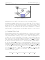
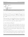
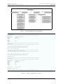
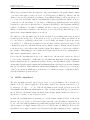
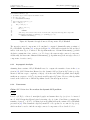
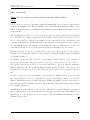
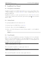
Figure 5 presents a partial class diagram for the framework. Each class of algorithms is implemented
as a subclass of GraphAlgorithm, which provides routines and data structures common to most
graph algorithms. From there, the abstract SCCAlgorithm and APSPAlgorithm classes provide
additional routines specialized for strongly-connected components and all-pairs shortest distance
algorithms, respectively. An additional class of algorithms can be implemented in the framework
simply by writing a new class that inherits from GraphAlgorithm, along with a factory class which
maps numeric identifiers specified on the command line to specific algorithms to be tested. For
instance, if a user executes the gbench application and specifies that SCC algorithm 1 should be
tested, then the get algorithm method in SCCAlgorithmFactory is called to obtain the algorithm
that maps to identifier 1.
As a result of the inheritance hierarchy employed within the framework, implementing a new algorithm of a given class is relatively simple. For instance, to implement a new SCC algorithm, one
need only write a class inheriting from SCCAlgorithm. A considerable amount of the code and data
structures needed by the algorithm is already present in the SCCAlgorithm and GraphAlgorithm
classes, diminishing development time. Once the algorithm has been implemented, one need only
make a small modification to the SCCAlgorithmFactory to allow the new algorithm to be instantiated by the gbench software.
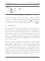
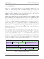
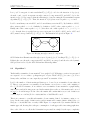
Figure 6 shows an execution of the gbench application, executing and validating the result of
Johnson’s algorithm [30] to compute the shortest path distances between all pairs of nodes in a
small graph. In addition to the features shown, the application allows one to execute multiple trials
of a given algorithm, specify a timeout after which a running algorithm will be interrupted, and
display the result of an algorithm, such as the distance matrix produced by an APSD algorithm.
16
Computer Science 9868
SPAWC: A Scalable Parallel Web Crawler
Jeffrey Shantz <jshantz(5-1)@csd.uwo.ca>
June 02, 2010
Figure 5: Partial GraphBench class diagram
================================================================================
Test Parameters
================================================================================
Algorithm Type
Algorithm
Graph
Vertices
Edges
Density
Trials
:
:
:
:
:
:
:
All - pairs shortest path
Johnson
Sanity Check 3
4
6
50%
1
================================================================================
Running trial 1
================================================================================
0%
10
20
30
40
50
60
70
80
90
100%
| - - - -| - - - -| - - - -| - - - -| - - - -| - - - -| - - - -| - - - -| - - - -| - - - -|
***************************************************
Trial 1 time : 00:00:00.000781
================================================================================
Validating algorithm - produced distance matrix
================================================================================
0%
10
20
30
40
50
60
70
80
90
100%
| - - - -| - - - -| - - - -| - - - -| - - - -| - - - -| - - - -| - - - -| - - - -| - - - -|
***************************************************
Validation passed
================================================================================
Final Report
================================================================================
Algorithm Type
Algorithm
Graph
Vertices
Edges
Density
Trials
:
:
:
:
:
:
:
All - pairs shortest path
Johnson
Sanity Check 3
4
6
50%
1
Trial 1 Time
: 00:00:00.000781
Validation Result : Passed
================================================================================
Figure 6: Sample GraphBench execution
17
Computer Science 9868
SPAWC: A Scalable Parallel Web Crawler
4.3
Jeffrey Shantz <jshantz(5-1)@csd.uwo.ca>
June 02, 2010
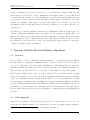
Graph File Format
As noted above, a GraphBench algorithm can be executed against any graph file specified on the
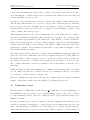
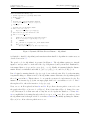
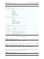
command line. Figure 7 shows the format of a GraphBench graph file. The file header begins
with a 10 byte magic number which indicates that the file contains a GraphBench graph. Next, a
null-terminated string provides a friendly name for the graph, which is displayed by gbench in its
summary (see Figure 6). The number of vertices, edges, and strongly-connected components in the
graph are then stored, each represented as 4 byte unsigned integers.
Originally, gbench validated the result of a graph algorithm by executing a well-known algorithm
against the graph in use, and comparing its result to that produced by the algorithm being tested.
However, for large graphs, this quickly became time consuming. To mitigate this problem, a
GraphBench graph file stores validation details directly within it. For instance, in a graph of
n nodes, the n × n distance matrix is stored within the file to allow the matrix produced by a
graph algorithm being tested to be quickly validated against the stored matrix. Next, a list of n
unsigned integers is stored, representing the index of the strongly-connected component in which
each vertex v0 , v1 , . . . , vn−1 ∈ V should belong. A merge components algorithm is provided in the
SCCAlgorithm class to ensure that all valid SCC algorithms compute the same SCC indices for
each vertex in a given graph.
The n × n adjacency matrix of the graph is then stored, followed by the edge insertion sequence
for the graph. Each edge is stored in 8 bytes, with the first 4 bytes storing the index of the source
vertex (tail), and the latter 4 bytes storing that of the target vertex (head). A vertex index is
represented as an unsigned integer i ∈ {0, 1, . . . , n − 1}. The gbench software iterates over the
edges stored, adding each edge in the sequence to the graph being used by a particular algorithm.
For instance, if one were testing some algorithm A, the first edge in the sequence would be added to
the graph, and A would then be executed on the modified graph. This process would then continue
for each edge in the insertion sequence, allowing dynamic algorithms to be tested over a sequence
of edge insertions.
Magic Number (10 bytes)
# Vertices (4 bytes)
# Edges (4 bytes)
Graph Name (Variable Length)
# SCCs (4 bytes)
\0
Distance Matrix (n x n x 4 bytes)
Vertex SCC Indices (n x 4 bytes)
Adjacency Matrix (n x n bytes)
Edge 1 (8 bytes)
...
...
Edge m (8 bytes)
Figure 7: GraphBench graph file format
The exception to this occurs when a batch algorithm is being tested, which is a dynamic algorithm
18
Computer Science 9868
SPAWC: A Scalable Parallel Web Crawler
Jeffrey Shantz <jshantz(5-1)@csd.uwo.ca>
June 02, 2010
capable of updating some property P given a set of edge insertions in a graph. In this case, the
user specifies a batch threshold t on the command line, indicating the number of edges that should
be inserted from the sequence before the algorithm is re-executed. gbench then inserts the next t
edges from the sequence and executes the algorithm, repeating the process until all edges in the
sequence are exhausted. If the number of edges in the sequence is not divisible by t, then the
algorithm is executed one last time after all edges have been inserted, to account for the last k < t
edges inserted.
One final note about the graph file format used by GraphBench is that it sacrifices space for
efficiency, duplicating information where it would provide an advantage in running time. For
instance, the format stores both the distance and adjacency matrices of a graph. This is unnecessary,
since either matrix could be computed using the other. This approach was avoided, however, since
the additional overhead involved in doing so far outweighs the meagre amount of extra space
consumed by simply storing both matrices.
5
Dynamic All-Pairs Shortest Distance Algorithms
5.1
Overview
Let G = (V, E) be a directed, unweighted graph such that |V | = n. The all-pairs shortest distance
problem is that of computing the minimum distance between each pair of vertices (v1 , v2 ), for
v1 , v2 ∈ V . Perhaps the best known static algorithms for solving this problem are the FloydWarshall algorithm [30], which solves the problem in O(n3 ) time, and Johnson’s algorithm [30],
which solves the problem in O(n2 log n + nm), where m is the number of edges in the graph1 .
In the dynamic variant of the problem, one seeks to update the shortest distance matrix of a graph
subject to the insertion of one or more edges. If the algorithm can handle the insertion of multiple
edges before updating its distance matrix, then it is said to be a batch algorithm. The following
sections present two singular insertion algorithms for solving the dynamic all-pairs shortest distance
problem. Additional singular insertion algorithms were implemented in GraphBench, but are not
presented here for brevity. Furthermore, although several batch algorithms were also implemented,
they are omitted as they did not provide clear advantages over singular insertion algorithms in tests
performed.
5.2
Naı̈ve Approach
Given a directed graph G = (V, E) and a new edge (u, v) to be inserted into E, for u, v ∈ V , one
can update the distance matrix of G by inserting the edge into the graph, and then running a
1
Assuming Fibonacci heaps are used when executing Dijkstra’s algorithm [30].
19
Computer Science 9868
SPAWC: A Scalable Parallel Web Crawler
Jeffrey Shantz <jshantz(5-1)@csd.uwo.ca>
June 02, 2010
well-known static algorithm such as Floyd-Warshall [30]. One can view the insertion of each edge
as producing a new static graph G0 , upon which the algorithm can be executed to compute an
updated distance matrix. Since the entire distance matrix for the graph would be recomputed,
taking into account the newly inserted edge, this approach correctly solves the dynamic all-pairs
shortest distance problem.
Of course, this naı̈ve approach is highly inefficient. If Floyd-Warshall is used, then each edge
insertion will require O(n3 ) time, where n is the number of vertices in the graph. Since a directed
graph can have up to O(n2 ) edges, the worst-case running time of this approach would be O(n5 )
over a sequence of O(n2 ) edge insertions, rendering it prohibitively inefficient.
5.3
Ausiello et al.
Ausiello et al. [31] present a recursive, incremental algorithm2 to solve the all-pairs shortest distance
problem for arbitrary directed graphs having positive integer edge weights. If the weight of each
edge in a graph is less than some constant C, then the algorithm requires O(Cn log n) amortized
running time per edge insertion. For unweighted graphs, such as the Web graph constructed by
SPAWC, edge insertions take place in O(n log n) amortized running time.
The algorithm works on the premise that the insertion of a new edge (i, j) into a graph G = (V, E)
can affect only the minimum distances between certain vertex pairs in V . If dold represents the
distance matrix of G, and dnew represents the matrix after the insertion of edge (i, j), then the
following holds:
dnew (x, y) = min{ dold (x, y), dold (x, i) + 1 + dold (j, y) }
∀x, y ∈ V
(1)
As noted in [31], equation 1 implies that the insertion of edge (i, j) can reduce the minimum distance
between a pair of vertices x, y ∈ V only if there exists some path x
i→j
y in G in which x
appears as a predecessor of i, and y appears as a successor of j. If either of these conditions do not
hold, then there is no path from x to y passing through edge (i, j), and so dnew (x, y) = dold (x, y).
Consequently, vertex pairs not meeting these conditions can be ignored when computing dnew ,
potentially eliminating a significant number of pairs that must be considered. Ausiello’s algorithm
capitalizes on this observation, maintaining two trees for each vertex v – DESC(v) and AN C(v)
– representing forward and backward minimal paths rooted at v, respectively. Additionally, an
n × n matrix F ORW ARD is maintained, such that F ORW ARD[u, v] contains a pointer to v in
DESC(u) if there exists a path from u to v, and NULL otherwise [31]. Similarly, an n × n matrix
BACKW ARD is also maintained to maintain pointers to the vertices in the ancestor trees of each
vertex in the graph. These matrices are used to provide constant time access to a particular vertex
in the descendant or ancestor tree of a given vertex.
2
Henceforth known as Ausiello’s algorithm
20
Computer Science 9868
SPAWC: A Scalable Parallel Web Crawler
Jeffrey Shantz <jshantz(5-1)@csd.uwo.ca>
June 02, 2010
When edge (i, j) is inserted into the graph, the only possible changes to the graph’s distance matrix
occur between the pairs of vertices (x, y) for x ∈ AN C(i) and y ∈ DESC(j). That is, only the
distance between i and j themselves can change, along with the distance between any ancestor of i
to j or any of its descendants. Ausiello’s algorithm thus begins by updating the distance from i to
j, and from i to all descendants of j. In doing so, DESC(i) is potentially updated, and AN C(v)
is updated for any vertex v that was added or updated in DESC(i). After updating DESC(i),
a subtree T will have been defined, containing only those vertices v for which d(i, v) decreased.
This tree is then passed recursively to the ancestors of i stored in AN C(i), which then proceed to
update their forward minimal path trees as well [31].
The efficiency of the algorithm comes from the fact that T is potentially pruned as it is passed
recursively up the ancestor tree. If the insertion of edge (i, j) does not change the distance from
i to some vertex v ∈ DESC(j), then it also does not change the distance between any vertex
u ∈ AN C(i) to v. This notion is captured by the fact that v will not appear in T , since T only
contains those vertices to which the current vertex’s distance changed. As such, when T is passed
to the ancestors of i, they will not unnecessarily compute their distance to vertex v since it will not
have changed. This pruning process continues as T is passed up the ancestor tree, assuring that no
unnecessary computations are carried out.
For brevity, the algorithm and its proof are omitted here, but interested readers are directed
to [31] for more information. Additionally, the algorithm was implemented in the GraphBench
framework and its source accompanies the package. As noted, the algorithm is capable of updating
an unweighted graph’s distance matrix (and all minimal path trees) in O(n log n) amortized running
time per edge insertion. This results in a total amortized running time of O(n3 log n) over a sequence
of O(n2 ) edge insertions. Furthermore, as it uses two n × n matrices, its space complexity is O(n2 ).
A detailed analysis is presented in [31].
5.4
APSD - Algorithm 1
The next algorithm presented was developed based on concepts similar to those presented by
Ausiello et al. [31]. Given a graph G = (V, E) with n vertices, we represent each vertex vi ∈ V
by an integer i ∈ {0, 1, . . . , n − 1}. Like the algorithm presented in the previous section, the
Algorithm1-Add-Edge algorithm makes use of the observation that if an edge (i, j) is inserted
into G, then the only distances that can change in the graph’s distance matrix are between i (or
any ancestor of i) and j or any of its predecessors.
As such, the algorithm starts by updating row i in the distance matrix D based on the newly
inserted edge (i, j). Next, for each vertex u that can reach i, the algorithm recomputes D[u, v]
∀v ∈ V . Of course, this algorithm is slower than that presented in the previous section, since it is
only necessary to recompute distances D[x, y] for x ∈ AN C(i) and y ∈ DESC(j). However, the
algorithm does not employ recursion, uses less memory (though its asymptotic space complexity
21
Computer Science 9868
SPAWC: A Scalable Parallel Web Crawler
Jeffrey Shantz <jshantz(5-1)@csd.uwo.ca>
June 02, 2010
APSD-Algorithm1-Add-Edge(src, tgt)
1 // If the edge from src to tgt already exists, return
2 if D[src, tgt] = = 1
3
return
4
5 // Update node count and the distance matrix D
6 node count = MAX{node count, src + 1, tgt + 1}
7 D[src, tgt] = 1
8
9 // Update row src in the distance matrix
10 for n = 0 to node count − 1
11
D[src, n] = MIN{D[src, n], 1 + D[tgt, n]}
12
13 // For each node, up to the current node count
14 for n1 = 0 to node count − 1
15
16
// Skip over src, tgt, and any node that cannot reach src
17
if (n1 = = src) or (n1 = = tgt) or (D[n1 , src] = = ∞)
18
continue
19
20
// n1 can reach src, so update row n1 in the distance matrix
21
for n2 = 0 to node count − 1
22
D[n1 , n2 ] = MIN{D[n1 , n2 ], D[n1 , src] + D[src, n2 ]}
Figure 8: Dynamic All-Pairs Shortest Distance - Algorithm 1
is identical to Ausiello’s algorithm), and runs faster than Ausiello’s algorithm in certain cases, as
described in section 5.5.
The pseudo-code for Algorithm 1 is presented in Figure 8. The algorithm requires two integral
inputs src and tgt, where src is the tail of the edge being inserted, and tgt is its head. Furthermore,
it is assumed that src 6= tgt, and src, tgt ∈ {0, 1, . . . n − 1}. Finally, it is assumed that the distance
matrix D has been initialized such that ∀i, j ∈ V, i 6= j, D[i, j] = ∞, and ∀i ∈ V, D[i, i] = 0.
Line 2 begins by ensuring that the edge (src, tgt) does not already exist. If it does, then inserting
it again will change no distances in D, so the algorithm returns. Otherwise, the algorithm updates
the node count in line 6. This is taken to be one past the greatest node index inserted so far. For
instance, if one inserts edge (5, 6) into an empty graph, then node count will store 6 + 1 = 7. Line 7
then updates D to reflect the insertion of edge (src, tgt).
Next, row src in D is updated in lines 10 and 11. If tgt offers a shorter path to some node n in
the graph, then D[src, n] is set to 1 + D[tgt, n]. Next, if any values D[src, v] changed for some
v ∈ V , then any node n1 that can reach src may also need to update its distance to v. Lines 14 to
22 accomplish this by iterating through each node n1 up to node count. If n1 can reach src, then
the algorithm iterates through each node n2 in lines 21 and 22, potentially updating the distance
D[n1 , n2 ] if src offers a shorter path from n1 to n2 .
22
Computer Science 9868
SPAWC: A Scalable Parallel Web Crawler
5.4.1
Jeffrey Shantz <jshantz(5-1)@csd.uwo.ca>
June 02, 2010
Asymptotic Analysis
The algorithm considers only nodes up to node count to save execution time by not attempting
to update rows in the distance matrix for vertices having indices higher than the current value
of node count. However, its asymptotic complexity for a single edge insertion is O(n2 ), since the
outer loop starting on line 14 runs n times, with its inner loop on line 21 also potentially running
n times. Consequently, a series of O(n2 ) edge insertions will run in O(n4 ) time in the worst case.
As with Ausiello’s algorithm, the space complexity of Algorithm 1 is O(n2 ), as it uses the n × n
distance matrix D.
5.4.2
Correctness
Claim: Algorithm 1 solves the dynamic all-pairs shortest distance problem
Proof:
Let G = (V, E) be an directed, unweighted graph, and suppose that we wish to insert edge (i, j)
such that i 6= j and i, j ∈ {0, 1, . . . , n − 1, where n = |V |.
To begin, one need consider the distances from i to j and every vertex v which j can reach. Trivially,
D[i, j] = 1. For each vertex v that j can reach, a new path p : i → j
this path, there may already be some path
p0
:i
v; j ∈
/
p0 .
v is created. In addition to
As such, we have the following two
cases.
Case 1: len(p0 ) < len(p)
In this case, j does not offer a shorter path to v, and so the distance D[i, v] should remain unchanged.
Algorithm 1 handles this case in line 11, since the min function will select the lowest distance, which,
in this case, will be the existing value of D[i, v].
Case 2: There is no existing path from i to v, or len(p) < len(p0 )
Here, j offers a shorter path to v, and so distance D[i, v] = D[i, j] + D[j, v] = 1 + D[j, v]. Again,
this is handled in line 11.
Hence, in either case, row i will be correctly updated in the distance matrix D. It now remains
to be shown that distances for all other affected vertices in the graph will be updated. Note that
a vertex u can only be affected by the insertion of edge (i, j) if u has a path to i. Otherwise,
this edge would have no bearing on the distance from u to any other node in the graph. As such,
the algorithm need only update distances from each vertex u that can reach i, to j and any of its
descendants.
Let u represent an ancestor of i, and v represent j or one of its descendants. As before, there are
two cases: either D[u, v] is already of minimal value, in which case it should remain unchanged, or
23
Computer Science 9868
SPAWC: A Scalable Parallel Web Crawler
Jeffrey Shantz <jshantz(5-1)@csd.uwo.ca>
June 02, 2010
edge (i, j) offers a shorter path from u to v, and thus D[u, v] = D[u, i] + 1 + D[j, v]. Equivalently,
since row i has already been updated in D, D[u, v] = D[u, i] + D[i, v]. Once again, these two cases
are handled by the loops in lines 14 to 22, and thus the distance from each ancestor of i to j or
any of its descendants will be properly updated in D.
Since all distances are properly updated in D after the insertion of edge (i, j), algorithm 1 correctly
solves the all-pairs shortest distance problem.
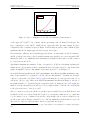
Execution Time (s)
102
101
Algorithm
Algorithm 1
Ausiello
10
0
10−1
1
2
3
4
5
6
Graph
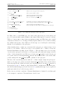
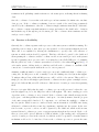
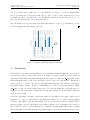
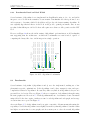
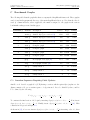
Figure 9: Singular APSD Algorithm Benchmarks
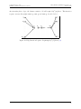
5.5
Benchmarks
Both Ausiello’s algorithm and Algorithm 1 were benchmarked using GraphBench on a variety of
edge insertion sequences (henceforth described as graphs for brevity), which are described fully in
Appendix C. Each APSD algorithm in GraphBench is required to define an add edge method that
takes as input the indices of the source and target vertices of the edge being inserted. This method
is then expected to add the edge into the algorithm’s internal graph data structure, and update
the graph’s distance matrix. As such, benchmarking proceeded for a given algorithm by calling
add edge for each edge in the graph being tested. For each algorithm and each graph tested, 3
trials were executed, and Figure 9 displays the average time required for an algorithm to insert all
edges in a given graph.
As shown, Algorithm 1 actually outperforms Ausiello’s algorithm on the sparse graphs tested
(graphs 1, 2, 5, and 6), with Ausiello’s algorithm performing best on complete graphs (graphs
3 and 4). Algorithm 1 performs particularly well on edge insertion sequences requiring Ω(n3 )
updates (graphs 1 and 2), with Ausiello’s algorithm requiring orders of magnitude more time for
these sequences. Moreover, informal memory consumption measurements taken while executing
the benchmarks revealed that Ausiello’s algorithm required a great deal of memory in some cases.
24
Computer Science 9868
SPAWC: A Scalable Parallel Web Crawler
Jeffrey Shantz <jshantz(5-1)@csd.uwo.ca>
June 02, 2010
For instance, in tests run on graph 5, the top utility showed that Ausiello’s algorithm consumed,
at its peak, over 31% of total system memory, while Algorithm 1 peaked at only 1.1% for the same
graph.
While the high memory consumption of Ausiello’s algorithm could be due to implementationdependent factors, and could likely be improved by converting it to an iterative algorithm, there
was insufficient time to investigate these possibilities. Thus, Algorithm 1 was chosen for use in
SPAWC to compute dynamic all-pairs shortest distances.
6
Dynamic Strongly-Connected Components Algorithms
Let G = (V, E) be a directed, unweighted graph such that |V | = n. A strongly-connected component
in G is a set of vertices VSCC ⊆ V such that, for each pair of vertices u, v ∈ VSCC , there exists a
path from u to v in G. The strongly-connected component problem, then, is that of partitioning
V into the collection of strongly-connected components present in G.
As before, in the dynamic variant of the SCC problem, one seeks to maintain such a partition as
edges are inserted into G. One can view a graph of n vertices and no edges as having n stronglyconnected components. Then, as edges are inserted into the graph and new paths are created, it is
possible that some existing strongly-connected components will be merged, reducing the number
of total components. As such, edge insertions can only reduce the number of strongly-connected
components in a graph.
The following sections present several singular insertion algorithms for solving the dynamic stronglyconnected component problem.
6.1
Naı̈ve Approach
Let G = (V, E) be a directed, unweighted graph having n vertices, and D be the shortest paths
distance matrix of G. Define T to be the transitive closure matrix of G as follows:

0 if u 6= v and D[u, v] = ∞,
T [u, v] =
1 otherwise
In other words, for some vertices u, v ∈ V , T [u, v] = 1 if and only if u = v or u has a path to
v in G. Thus, the row in T corresponding to vertex u will contain the value 1 in each column
corresponding to vertices to which it has a path. Consequently, this matrix can then be utilized
to determine the strongly-connected components of G. Observe that, for some vertices u, v ∈ V , if
T [u, v] = T [v, u] = 1, then u and v have a path to each other, and thus form a strongly-connected
component.
25
Computer Science 9868
SPAWC: A Scalable Parallel Web Crawler
Jeffrey Shantz <jshantz(5-1)@csd.uwo.ca>
June 02, 2010
SCC-Naı̈ve-Add-Edge(src, tgt)
1 // Add the edge to G and compute its transitive closure
2 E = E ∪ {(src, tgt)}
3 T = Transitive-Closure(G)
4
5 // For each pair of vertices i, j ∈ V
6 for i = 0 to |V | − 1
7
for j = 0 to |V | − 1
8
9
// Move on if i == j
10
if i = = j
11
continue
12
13
// If i and j can reach each other, and are not in the same component, then merge their components
14
if ((!Same-Component(i, j)) and (T [i, j] = = 1) and (T [j, i] = = 1))
15
Merge-Components(i, j)
Figure 10: Dynamic Strongly-Connected Components - Floyd-Warshall
The strongly-connected components of G can thus be computed dynamically using a variant of
Floyd-Warshall’s algorithm [30], as shown in Figure 10, which takes as input the tail and head
indices of the next edge to be inserted. The algorithm makes use of Same-Component(i, j), which
checks in constant time if two vertices i, j ∈ V belong to the same strongly-connected component.
Additionally, the linear time Merge-Components(i, j) algorithm merges the strongly-connected
components of vertices i and j.
6.1.1
Asymptotic Analysis
Assuming that a variant of Floyd-Warshall is used to compute the transitive closure in line 3, as
given in [30], SCC-Naı̈ve-Add-Edge solves the dynamic SCC problem in O(n3 ) time per edge
insertion, and has a space complexity of Θ(n2 ). As in the naı̈ve APSD algorithm, this is highly
inefficient as a sequence of O(n2 ) edge insertions will require O(n5 ) time. However, this algorithm
is used as the basis for more efficient algorithms described in subsequent sections.
6.1.2
Correctness
Claim: SCC-Naı̈ve-Add-Edge solves the dynamic SCC problem
Proof:
Let G = (V, E) be a directed, unweighted graph, and assume that edge (u, v) is to be inserted
into G. SCC-Naı̈ve-Add-Edge begins by inserting edge (u, v) into G and then recomputing the
transitive closure G∗ = (V, E ∗ ) of G using a given algorithm, such as the variant of Floyd-Warshall
presented in [30]. This returns the adjacency matrix T of G∗ , updated to account for edge (u, v),
which can then be used to find the strongly-connected components of G as described below.
26
Computer Science 9868
SPAWC: A Scalable Parallel Web Crawler
Jeffrey Shantz <jshantz(5-1)@csd.uwo.ca>
June 02, 2010
Let i, j ∈ V be any pair of vertices such that T [i, j] ∧ T [j, i] = 0 before the insertion of edge (u, v).
As such, i and j reside in separate strongly-connected components SCCi and SCCj before the
insertion of (u, v). Now, suppose that after inserting (u, v) and executing the Transitive-Closure
algorithm, T [i, j] = T [j, i] = 1. Then, the insertion of (u, v) has created a path i
j
i in G.
Let k be an arbitrary vertex in SCCi , and ` be an arbitrary vertex in SCCj . By definition of SCCi ,
there exists a path k
i
k. Similarly, by definition of SCCj , there exists a path `
Finally, since there exists a path i
i
j
i, then there also exists a path k
i
j
j
`
`.
j
k. As such, there is a path between every vertex pair k, ` ∈ SCCi ∪ SCCj , and so SCCi and
SCCj must be merged when T [i, j] = T [j, i] = 1. This situation is depicted in Figure 11.
i
SCC i
j
SCC j
Figure 11: Merging strongly-connected components
SCC-Naı̈ve-Add-Edge iterates through every node pair (i, j) ∈ V , checking if T [i, j] = T [j, i] = 1.
If this is the case, then the components SCCi and SCCj are merged, and therefore the dynamic
SCC problem is solved by the SCC-Naı̈ve-Add-Edge algorithm.
6.2
Algorithm 1
Traditionally, a transitive closure matrix T for a graph G = (V, E) having n vertices is represented
as a sequence of n × n values – perhaps integers or bytes. Each cell T [i, j] for some i, j ∈ V is a
binary value, and thus one can compactly represent T as a matrix of bits.
Let b be the number of bits in an integral data type to be used to store transitive closure values in
T . Then, to represent an n × n transitive closure matrix, one need store n rows, each consisting of
B = d nb e blocks. For instance, if one wishes to store a transitive closure matrix for a graph having
2000 vertices, and 64 bit integers are used in the matrix, then each row of the matrix can be stored
in d 2000
64 e = 32 64-bit integer blocks. Since the matrix will contain 2000 rows, a total of 2000 rows
× 32 blocks/row × 64 bits/block = 4, 096, 000 bits or 500 KB will be used.
This is in contrast to a traditional transitive closure matrix defined, for instance, using n × n
bytes. In the same graph of 2000 vertices, such a matrix will consume (2000 × 2000) bytes × 8
bits/byte = 32, 000, 000 bits or nearly 4 MB. Figure 12 compares the byte matrix with the bit
matrix approach, showing the total space consumption of each approach for increasing graph sizes.
Since each of the n × n cells in the bit matrix is represented in a single bit, the space complexity
27
Jeffrey Shantz <jshantz(5-1)@csd.uwo.ca>
June 02, 2010
60
Computer Science 9868
SPAWC: A Scalable Parallel Web Crawler
40
30
20
0
10
Memory Usage (GB)
50
Square Matrix
Bit Matrix
0
50000
100000
150000
200000
250000
Vertices
Figure 12: Space consumption of bit- and byte-transitive closure matrices
of the approach3 is O(n2 ). By contrast, when representing each cell using b-bit integers, the
space complexity becomes O(bn2 ). While the two approaches have the same asymptotic space
complexities if the constant b is ignored, Figure 12 shows that, in practice, this constant is quite
significant, and the bit matrix approach saves a great deal of space.
Beyond its space efficiency, the bit matrix approach can save execution time as well. For instance,
an OR operation between two b-bit blocks in the matrix can generally be processed in a single CPU
instruction, while to accomplish the same task using a byte matrix would require one OR operation
for every vertex in the block.
Algorithm 1 maintains the transitive closure of a graph G = (V, E) as a bit matrix, updating the
matrix as new edges as inserted, and recomputing the list of strongly-connected components in the
graph. A simplified version of Algorithm 1 is presented in pseudo-code in Figure 13.
As in SCC-Naı̈ve-Add-Edge, the SCC-Algorithm1-Add-Edge algorithm maintains a transitive closure matrix T for a graph G = (V, E), and uses this matrix to determine the stronglyconnected components of G. Lines 2 and 3 begin by inserting the src and tgt vertices into G, as
well as the edge (src, tgt). Then, as in APSD-Algorithm1-Add-Edge in Figure 8, the size of
the graph is taken to be 1 past the largest vertex index in the G. Using the size of the graph, the
number of blocks currently used in each row of T is computed in line 7, and the bit corresponding
to the vertex tgt is set to 1 in row src in T .
Since src can now access tgt, it can also access any vertices reachable by tgt. As such, lines 11 and
12 OR the blocks of row tgt in T with the blocks of src, storing the results in row src. After this
loop is complete, row src contains a 1 in each bit corresponding to those vertices reachable by tgt,
as well as any vertices already reachable by src. The algorithm then checks in line 15 if tgt can
also reach src, and, if so, their strongly-connected components are merged.
3
Some internal fragmentation may occur due to space wasted when n is not divisible by b, but this bound is quite
close.
28
Computer Science 9868
SPAWC: A Scalable Parallel Web Crawler
Jeffrey Shantz <jshantz(5-1)@csd.uwo.ca>
June 02, 2010
SCC-Algorithm1-Add-Edge(src, tgt)
1 // Add the src and tgt vertices, and the edge (src, tgt)
2 V = V ∪ {src, tgt}
3 E = E ∪ {(src, tgt)}
4
5 // Update the current size of the graph, and compute the number of blocks currently used
6 size = max{v | v ∈ V } + 1
7 blocks = dsize/bitse
8 Set the bit corresponding to tgt in row T [src]
9
10 // OR the blocks of tgt with those of src
11 for i = 0 to blocks − 1
12
T [src, i] |= T [tgt, i]
13
14 // If src and tgt can reach each other, merge their components
15 if Can-Reach(tgt, src)
16
Merge-Components(src, tgt)
17
18 // Iterate over each vertex currently in the graph
19 for n = 0 to size − 1
20
21
// If the next vertex n can reach src
22
if ((n 6= src) and (n 6= tgt) and (Can-Reach(n, src)))
23
24
// OR the blocks of src with those of n
25
for i = 0 to blocks − 1
26
T [n, i] |= T [src, i]
27
28
// If src can also reach n, merge their components
29
if ((Can-Reach(src, n)) and (!Same-Component(src, n)))
30
Merge-Components(src, n)
Figure 13: Dynamic Strongly-Connected Components - Algorithm 1
Next, the predecessors of src must be updated since any vertices newly reachable by src through
tgt are also reachable by all predecessors of src. The loop starting on line 19 iterates over each
predecessor n of src, OR-ing the blocks of src with the blocks of n, and storing the result in row
n in T . After updating row n in T , the algorithm checks in line 29 if src can also reach n. If so,
then their strongly-connected components are merged.
6.2.1
Asymptotic Analysis
The running time of SCC-Algorithm1-Add-Edge is dominated by the loop starting on line 19.
n
) = O(n) time.
This loop runs O(n) times, while the inner loop starting on line 25 runs in O( bits
Furthermore, as noted earlier, Merge-Components runs in O(n) time, and thus the worst-case
running time of SCC-Algorithm1-Add-Edge is O(n2 ).
As discussed above, the space complexity of the algorithm is Θ(n2 ), as it uses 1 bit for each of the
n × n cells in the transitive closure matrix.
29
Computer Science 9868
SPAWC: A Scalable Parallel Web Crawler
6.2.2
Jeffrey Shantz <jshantz(5-1)@csd.uwo.ca>
June 02, 2010
Correctness
Claim: SCC-Algorithm1-Add-Edge solves the dynamic SCC problem
Proof:
Let G = (V, E) be a directed, unweighted graph, and assume that edge (u, v) is to be inserted into
G. SCC-Algorithm1-Add-Edge is similar to the SCC-Naı̈ve-Add-Edge algorithm, except
that it combines the steps of maintaining the transitive closure matrix and strongly-connected
component list.
The algorithm first sets T [u, v] = 1. Since u can now reach v, u can also reach all vertices reachable
by v, and thus row u must be updated in T accordingly. Observe that, for any vertex k ∈ V ,
W
T [u, k] = T [u, k] T [v, k]. That is, k is reachable by u if v can reach k, or if u could already reach
k directly or through some other intermediary vertex. As such, each bit bu in row u can be updated
W
by computing the binary OR with the corresponding bit bv in row v, such that bu = bu bv . By
doing this for all bits in row u, T will contain an updated reachability vector for vertex u.
Given the insertion of edge (u, v), we have that u can reach v. However, if v can also reach u,
then, as before, the strongly-connected components SCCu and SCCv must be merged, and this is
accomplished in line 15.
It remains to update all other rows in T corresponding to vertices affected by the insertion of
edge (u, v). Observe that, after the insertion of edge (u, v), for any vertices k, ` ∈ V , T [k, `] =
W
V
T [k, `] (T [k, u] T [u, `]). If T [k, `] = 1 before the insertion of edge (u, v), then it remains unV
changed. Otherwise, the only way it can change is if (T [k, u] T [u, `]) is true. Since T [k, u] = 1 if
and only if k is a predecessor of u, it follows that only rows for predecessors of u must be updated
in T .
As before, each predecessor k of u has its row in T updated by OR-ing each bit bk in row k with
W
the corresponding bit bu in row u, such that bk = bk bu . After this is complete, row k in T is
updated with any new vertices reachable through u. Finally, it remains to check if u can reach k. If
this is the case, then the strongly-connected components SCCu and SCCk must be merged, which
is accomplished in line 30.
As such, after all predecessors k of u are processed, all affected rows in T will have been updated
based on the insertion of edge (u, v), and the list of strongly-connected components will have been
updated based on the updated version of T . Hence, SCC-Algorithm1-Add-Edge solves the
dynamic SCC problem.
30
Computer Science 9868
SPAWC: A Scalable Parallel Web Crawler
6.2.3
Jeffrey Shantz <jshantz(5-1)@csd.uwo.ca>
June 02, 2010
Benchmarks Based on Block Width
Several variants of Algorithm 1 were implemented in GraphBench, using 8-, 16-, 32-, and 64-bit
integers to store blocks in the transitive closure matrix. Benchmarks were then performed on a
32-bit system to determine which block width would produce the fastest running algorithm. It
was originally hypothesized that a 32-bit block would provide optimal performance since it was
speculated that OR-ing two 64-bit blocks would require more than one OR operation at the CPU
level.
However, as Figure 14 shows, the 64-bit variant of Algorithm 1 performs fastest on all benchmarks
run, suggesting that the architecture on which the benchmarks were run is indeed capable of
computing the binary OR of two 64-bit integers in a single operation.
Execution Time (s)
2.25
Block Width
1.00
8
16
32
64
0.25
0.00
1
2
3
4
5
6
Graph
Figure 14: SCC - Algorithm 1 benchmarks
6.3
Benchmarks
Several variants of algorithm 1 (algorithms 2 and 3) were also implemented, making use of implementation specific optimizations. Both algorithms 2 and 3 have asymptotic time and space
complexities identical to algorithm 1. Because they differ very little from algorithm 1, they are not
presented here for brevity. However, Figure 15 shows a comparison of algorithms 1 through 3 using
the same graphs tested in section 5.5. Each algorithm makes use of a transitive closure bit matrix
using 64-bit blocks. Once again, 3 trials were run for each algorithm and each graph, and average
execution times are reported in Figure 15.
As seen in Figure 15, both algorithms 2 and 3 are quite competitive. Measurements taken using the
top utility revealed that Algorithm 3 uses slightly less memory than Algorithm 2, but this results
in a higher execution time for some graphs, as it frees memory more often. As a result, Algorithm
31
Computer Science 9868
SPAWC: A Scalable Parallel Web Crawler
Jeffrey Shantz <jshantz(5-1)@csd.uwo.ca>
June 02, 2010
Execution Time (s)
0.64
0.36
Algorithm
Algorithm 1
Algorithm 2
Algorithm 3
0.16
0.04
0.00
1
2
3
4
5
6
Graph
Figure 15: SCC benchmarks
2 was selected for use in SPAWC since it is quite simple, and provides excellent performance.
7
Maintaining Statistics for the SPAWC Web Graph
As noted, APSD Algorithm 1 from section 5.4 was chosen to maintain the dynamic all-pairs shortest
distances of the crawled Web graph in SPAWC, while SCC Algorithm 2 was selected (similar to
SCC Algorithm 1 in section 6.2) to maintain the list of strongly-connected components.
For each edge inserted into the Web graph, a slightly modified version of APSD Algorithm 1 is
called to update the distance matrix of the graph. In this modified variant, a max-priority queue
implemented using a Fibonacci heap stores all values from the distance matrix of the graph. Since
the diameter of a graph is defined to be the longest shortest path between any two nodes in the
graph, obtaining the diameter of the graph can be done in constant time by examining the maximum
value in the priority queue.
To maintain the priority queue, each time the distance between two vertices i, j is reduced, the
algorithm first removes Dold (i, j) and replaces it with Dnew (i, j). Removing a value from a Fibonacci
heap takes place in O(log n) time, while inserting a value can be done in constant time [30]. This
update procedure raises the running time of APSD Algorithm 1 to O(n2 log n), but allows the graph
diameter to be queried in constant time.
Next, SCC Algorithm 2 is called to update the list of strongly-connected components in the graph.
Each time the Merge-Components algorithm is called, a counter storing the current number of
strongly-connected components in the graph is decremented, allowing this number to be queried in
constant time.
32
Computer Science 9868
SPAWC: A Scalable Parallel Web Crawler
Jeffrey Shantz <jshantz(5-1)@csd.uwo.ca>
June 02, 2010
Finally, the degrees of the graph are updated based on the edge inserted in constant time. For
instance, if edge (u, v) is inserted into the graph, then the out-degree of u is incremented by 1,
while the in-degree of v is similarly incremented.
Consequently, the total execution time required for a single edge insertion into the Web graph is
O(n2 log n), producing a total running time of O(n4 log n) over a sequence of O(n2 ) edge insertions.
33
Computer Science 9868
SPAWC: A Scalable Parallel Web Crawler
Jeffrey Shantz <jshantz(5-1)@csd.uwo.ca>
June 02, 2010
Part III
Conclusions
8
8.1
Related Work
Web Crawling
Cho and Garcia-Molina [32] present an overview of issues relating to the design of a parallel Web
crawler, proposing metrics to evaluate crawlers, and providing a comparison of several crawler
architectures. Hafri and Djeraba [33] discuss the Erlang-based Dominos parallel Web crawler,
which is capable of crawling thousands of pages per second using Erlang worker processes.
The WebGraph framework [7] offers data structures and algorithms for static Web graph analysis,
capable of reading graphs from various sources, including those generated by the parallel UbiCrawler
[34]. WebGraph employs novel graph compression techniques, allowing metrics to be computed
efficiently on massive Web graphs.
8.2
Dynamic Graph Algorithms
Buriol et al. [35] present an excellent survey of dynamic APSP algorithms. In addition to proposing
a technique to reduce the size of heaps employed in numerous APSP algorithms, they present comprehensive benchmarks of several dynamic APSP algorithms due to Demetrescu [36], Ramalingam
and Reps [37], and King and Thorup [38], using a variety of graph insertion sequences.
Demetrescu and Italiano [26] give a fully dynamic algorithm for solving the all-pairs shortest path
problem in O(n2 log3 n) amortized time per graph update. Their algorithm works on arbitrary
directed graphs having non-negative, real-valued edge weights, and makes use of the notion of
locally shortest paths to reduce the time needed to process graph updates.
Yellin [39] presents an incremental algorithm to maintain the transitive closure G∗ = (V, E ∗ ) of a
graph G = (V, E), supporting edge insertions in O(dm∗ ) time, where d is the maximum out-degree
in the final graph, and m∗ = |E ∗ |, the number of edges in the final transitive closure of G. A variant
of this algorithm was implemented in the GraphBench framework to maintain strongly-connected
components in a dynamic graph, but insufficient time was available to ensure that the algorithm
worked properly on all classes of graphs.
Katz and Kider [40] give an efficient algorithm for solving both all-pairs shortest path and transitive
closure problems on large, static graphs. Their solution exploits the parallel capabilities of the
NVIDIA G80 GPU architecture, and although it was not designed as a dynamic algorithm, it is
feasible that adding parallelism to a dynamic graph algorithm could greatly increase the size of
34
Computer Science 9868
SPAWC: A Scalable Parallel Web Crawler
Jeffrey Shantz <jshantz(5-1)@csd.uwo.ca>
June 02, 2010
graphs that could be processed.
9
Conclusions and Future Work
SPAWC offers a high-performance, scalable architecture for Web crawling, making use of lowlatency MQ servers to facilitate efficient, simplified communication among potentially thousands of
crawler processes. Additionally, SPAWC provides a novel user interface which presents near realtime metrics on the crawled Web graph, as computed using numerous dynamic graph algorithms.
As discussed in section 2.8, there are potential barriers to scalability that need to be addressed in
future work. Specifically, the architecture must be augmented to support the presence of multiple
MQ servers, in addition to multiple coordinator processes. This would also require a means of
efficient synchronization between multiple coordinators.
Furthermore, while dynamic graph statistics are convenient, maintaining them online presents a
significant barrier to scalability. Future work could focus on techniques for efficient, offline analysis,
as well as techniques to compress and mine stored Web graphs.
35
Computer Science 9868
SPAWC: A Scalable Parallel Web Crawler
Jeffrey Shantz <jshantz(5-1)@csd.uwo.ca>
June 02, 2010
Appendices
A
A.1
SPAWC User Manual
Prerequisites
As several packages needed by SPAWC are not provided in the UWO environment, SPAWC is
provided within a virtual machine (VM). The SPAWC VM is compatible with the freely-available
VMware Player, as well as VMware Workstation 5.0 and above. VMware Player is installed on lab
machines in Middlesex College 342, and can also be downloaded freely from the VMware Web site
[41]. Note that registration is required in order to download the software, but there is no charge
for this process. For assistance with installing the software, consult the documentation available
on [41] for the platform on which VMware Player is being installed.
A.2
Getting Started
The following instructions detail the process of starting the SPAWC virtual machine. Please ensure
that VMware Player has been installed on the system on which SPAWC is to be run.
A.1 Insert the USB key containing the SPAWC VM into a free USB port
A.2 Launch the VMware Player application
A.3 If a License Agreement window appears, accept the terms of the agreement and click OK
A.4 Select Open from the main VMware Player window
A.5 In the dialog that appears, browse to the USB key, and select cs9868.vmx
A.6 Click the Open button to start the virtual machine
A.7 When the boot process completes, you should be taken to the GNOME desktop
A.8 If at any time you are prompted for a username or password, use the following credentials:
• Username: cs9868
• Password: algorithms
A.9 Double-click on the SPAWC icon on the desktop to launch the Web dashboard
Note: Running the SPAWC VM from the USB key greatly impacts its performance. For best
results, copy the contents of the USB key to a local disk before executing SPAWC.
36
Computer Science 9868
SPAWC: A Scalable Parallel Web Crawler
Jeffrey Shantz <jshantz(5-1)@csd.uwo.ca>
June 02, 2010
Tips: For convenience, one can press Ctrl+Alt+Enter to enter full screen mode in VMware Player.
At any time, this mode can be exited by pressing the same key sequence again. Additionally,
VMware Player may be configured to “lock” one’s mouse and keyboard into the virtual machine.
To unlock them, press Ctrl+Alt at any time.
A.3
Starting a Crawl
To begin a crawl session, follow the instructions below.
A.1 Select the Crawler Setup tab
A.2 Choose the initial number of crawler processes to spawn using the Initial Crawler Processes
slider
A.3 Select the number of URLs to crawl using the Max. URLs to Crawl slider
A.4 In the Add Seed URL field, enter a URL at which to begin crawling and click the Add
button. Multiple seed URLs can be added, if desired
A.5 To begin crawling, click the Start button
Figure 16 shows the Crawler Setup tab before a crawl is initiated. Once the Start button is clicked,
the Crawler Status tab will appear, allowing one to monitor the progress of the crawl.
Figure 16: Crawler Setup tab
37
Computer Science 9868
SPAWC: A Scalable Parallel Web Crawler
A.4
Jeffrey Shantz <jshantz(5-1)@csd.uwo.ca>
June 02, 2010
Monitoring a Crawl
Figure 17 shows the Crawler Status tab, displaying the progress of an ongoing crawl. The following
subsections describe the various panes found on this tab.
Figure 17: Crawler Status tab
A.4.1
Coordinator Pane
The Coordinator pane appears on the left side of the Crawler Status tab, as shown in Figure 17.
This pane provides details on the current status of the crawler, its process ID, and the progress of
the crawl expressed as a percentage of the maximum URLs specified.
The Coordinator pane also allows one to tune the crawl rate by adjusting the number of active
crawler processes. To change this number, drag the Processes slider to the desired value. Within
a few seconds, the change should be visible in the Crawlers pane.
Finally, at any time during an active crawl session, one can choose to terminate the crawl by clicking
the Stop button, located at the bottom of the Coordinator pane. Note that this may take several
seconds to complete, as the coordinator and all crawler processes are shut down.
A.4.2
Crawlers Pane
Figure 17 shows the Crawlers pane in the center of the Crawler Status tab. This pane provides
near real-time information on the current status of each crawler process. The crawler processes are
displayed in tabular form, with the following information presented for each process:
• ID: A numeric ID assigned to the crawler process by the coordinator
38
Computer Science 9868
SPAWC: A Scalable Parallel Web Crawler
Jeffrey Shantz <jshantz(5-1)@csd.uwo.ca>
June 02, 2010
• Process ID: The process ID assigned to the crawler process by the operating system
• Status: A message describing the current state of the process
• Last Updated: The time at which the last status update was received from the crawler
A.4.3
Statistics Pane
As shown in Figure 17, the Statistics pane is presented on the right side of the Crawler Status
tab. In this pane, statistics on the active crawl are presented in near real-time, refreshed every few
seconds as the dashboard communicates with the coordinator process. The following metrics are
presented in the Statistics pane:
• Crawl Time: Time elapsed during an active crawl
• URLs/second: Number of URLs downloaded per second (crawl rate)
• Download Size: Total page bytes downloaded
• Throughput: Page download throughput
• Max. URLs: Maximum number of URLs selected for the active crawl
• URLs Crawled: Number of URLs crawled successfully
• URL Errors: Number of failed crawl attempts
• Total URLs: URLs Crawled + URL Errors
• SCC Count: Number of strongly-connected components in the Web graph
• Dangling Nodes: Number of nodes having no outbound edges in the Web graph
• Graph Diameter: Diameter of the Web graph
• Average Distance: Average distance between any two vertices in the Web graph
A.4.4
Degree Distributions Pane
The Degree Distributions pane is located at the bottom of the Crawler Status tab, as shown in
Figure 17. This pane displays frequency distributions for the inbound and outbound degrees of the
vertices of the crawled Web graph.
39
Computer Science 9868
SPAWC: A Scalable Parallel Web Crawler
A.5
Jeffrey Shantz <jshantz(5-1)@csd.uwo.ca>
June 02, 2010
Diagnostics
As discussed in section 2.6, the coordinator and crawler processes periodically log status messages
to disk, allowing for more detailed information to be obtained than that presented on the Web dashboard. All logs are available in the SPAWC VM in the directory /home/cs9868/crawler/lib/logs.
Previously, these logs were viewable from the dashboard, but this functionality was removed as refreshing the logs consumed too many server resources.
40
Computer Science 9868
SPAWC: A Scalable Parallel Web Crawler
B
B.1
Jeffrey Shantz <jshantz(5-1)@csd.uwo.ca>
June 02, 2010
GraphBench User Manual
Prerequisites and Installation
GraphBench is installed in the SPAWC virtual machine and, as such, requires VMware Player
or VMware Workstation. See sections A.1 and A.2 for details on installing VMware Player and
starting the SPAWC VM.
GraphBench also makes use of certain components in the Boost C++ libraries [42]. Boost v1.42.0
or greater must be installed in the system include path, with the program options and thread
libraries compiled.
B.2
Getting Started
To begin using GraphBench, follow the instructions below.
B.1 Start and login to the SPAWC VM (see section A.2)
B.2 From the desktop, double-click the GraphBench icon
B.3 In the console window that appears, enter the following command to see the GraphBench
usage screen:
./gbench
B.3
Usage Examples
Figure 18 reproduces the GraphBench program usage. All graphs provided for use with GraphBench are located in the graphs subdirectory of the main GraphBench directory. The following
examples demonstrate the use of GraphBench and its various features. Note that GraphBench can
be terminated at any time by pressing Ctrl+C.
Example 1: Executing an APSP algorithm
./gbench --graph graphs/c100.g --apsp 3
This executes Ausiello’s algorithm on a complete graph of 100 nodes.
Example 2: Executing a SCC algorithm
./gbench --graph graphs/c100.g --scc 7
This executes SCC Algorithm 1 on the same complete graph of 100 nodes.
41
Computer Science 9868
SPAWC: A Scalable Parallel Web Crawler
Jeffrey Shantz <jshantz(5-1)@csd.uwo.ca>
June 02, 2010
Usage : gbench -- graph GRAPH_FILE [ - - apsp | -- scc ] ALGORITHM [ OPTIONS ]
Required options :
-g [ -- graph ] arg
Specify the graph file to use
All - pairs shortest path options :
-a [ -- apsp ] arg
Run the program using an all - pairs shortest path
algorithm .
Valid algorithms :
1: Floyd - Warshall
2: Johnson
3: Ausiello
4: Algorithm 1
5: Algorithm 2
6: Floyd - Warshall ( Batch )
7: Johnson ( Batch )
8: Algorithm 3 ( Batch )
9: Algorithm 4 ( Batch )
Strongly - connected components options :
-s [ -- scc ] arg
Run the program using a strongly - connected component
algorithm
Valid algorithms :
1: Floyd - Warshall
2: Tarjan
3: Yellin
4: Algorithm 1 (8 bits / block )
5: Algorithm 1 (16 bits / block )
6: Algorithm 1 (32 bits / block )
7: Algorithm 1 (64 bits / block )
8: Algorithm 2 (64 bits / block )
9: Algorithm 3 (64 bits / block )
Batch algorithm options :
-t [ -- threshold ] arg Maximum number of edge insertions before the algorithm
is executed
Conversion options :
-c [ -- convert ] arg1 arg2
-n [ -- name ] arg
Generic options :
-r [ -- trials ] arg
-o [ -- timeout ] arg
-v [ -- validate ]
-p [ -- print - matrices ]
-h [ -- help ]
Convert dimacs_file ( arg1 ) to a GraphBench graph
file ( arg2 )
Graph name
Number of times to run the algorithm
Maximum time ( in seconds ) to allow an algorithm to
run
Validates the result produced by the algorithm in
use after all edges have been inserted
Print the distance / SCC matrices computed ( not
recommended for large graphs )
Show this help message
Figure 18: GraphBench usage
Example 3: Running multiple trials
./gbench --graph graphs/c100.g --apsp 3 --trials 3
This executes the same benchmark as in Example 1, but executes three trials for the benchmark.
Example 4: Validating and printing algorithm output
./gbench --graph graphs/sc1.g --apsp 3 --validate --print-matrices
Executes Ausiello’s algorithm on a small graph, validating its final distance matrix against that
stored in the graph file, and printing the final distance matrix.
Example 5: Specifying a timeout
./gbench --graph graphs/c100.g --apsp 1 --timeout 10
42
Computer Science 9868
SPAWC: A Scalable Parallel Web Crawler
Jeffrey Shantz <jshantz(5-1)@csd.uwo.ca>
June 02, 2010
Executes the Floyd-Warshall algorithm after each edge inserted into a complete graph of 100 vertices, timing out if the algorithm does not complete within 10 seconds.
43
Computer Science 9868
SPAWC: A Scalable Parallel Web Crawler
C
Jeffrey Shantz <jshantz(5-1)@csd.uwo.ca>
June 02, 2010
Benchmark Graphs
The following table lists the graph files that accompany the GraphBench framework. These graphs
can be found in the graphs subdirectory of the main GraphBench directory. Note that the Benchmark # column indicates, where applicable, the number assigned to the graph in the various
benchmark results presented in this paper.
Benchmark #
Filename
Description
Vertices
Edges
Density
a1500.g
Ausiello Ω(n3 ) (see section C.1)
1500
1997
0.09%
1
a300.g
Ausiello Ω(n3 ) (see section C.1)
300
397
0.44%
2
a900.g
Ausiello Ω(n3 ) (see section C.1)
900
1197
0.15%
3
c100.g
Complete graph
100
9900
100.00%
c200.g
Complete graph
200
39800
100.00%
c400.g
Complete graph
400
159600
100.00%
c800.g
Complete graph
800
639200
100.00%
5
ga.g
Road graph of Georgia [43]
1557
5016
0.21%
6
id.g
Road graph of Idaho [43]
256
672
1.03%
sc1.g
Sanity Check 1
8
11
19.64%
sc2.g
Sanity Check 2
8
14
25.00%
sc3.g
Sanity Check 1
4
6
50.00%
4
C.1
Insertion Sequences Requiring Cubic Updates
Ausiello et al. describe a graph G = (V, E) having n vertices which requires Ω(n3 ) updates to the
distance matrix of G over a certain sequence of edges inserted. Let n be divisible by three, and let
V be defined by the following:
V = {s1 , s2 , . . . , s n3 , x1 , x2 , . . . , x n3 , t1 , t2 , . . . , t n3 }
To construct the final version of G, begin by inserting edges (si , x1 ) for i = 1, 2, . . . , n3 . Next, insert
edges (xi , xi+1 ) for i = 2, 3 . . . , n3 − 1. Finally, insert edges (x n3 , ti ) for i = 1, 2, . . . , n3 [31]. This
construction is depicted in Figure 19.
As shown in [31], if one now inserts edges (x1 , xi ) for i = 2, 3, . . . , n3 in increasing order of i, then
44
Computer Science 9868
SPAWC: A Scalable Parallel Web Crawler
Jeffrey Shantz <jshantz(5-1)@csd.uwo.ca>
June 02, 2010
after inserting these edges, the distance matrix of G will require Ω(n3 ) updates. This insertion
sequence was used in graphs a1500.g, a300.g, and a900.g, described above.
Figure 19: Edge Insertion Sequence Requiring Ω(n3 ) Updates [31]
45
Computer Science 9868
SPAWC: A Scalable Parallel Web Crawler
D
Jeffrey Shantz <jshantz(5-1)@csd.uwo.ca>
June 02, 2010
References
[1] J. Alpert and N. Hajaj. (Jul 2008) We knew the web was big... The Official Google Blog.
[Online]. Available:
http://googleblog.blogspot.com/2008/07/we-knew-web-was-big.html
[Accessed: 10 May 2010]
[2] J. Markoff. (Sep 2005) How Many Pages in Google?
Take a Guess. The New York
Times. [Online]. Available: http://www.nytimes.com/2005/09/27/technology/27search.html
[Accessed: 10 May 2010]
[3] A. King. (May 2008) The Average Web Page. OptimizationWeek.com. [Online]. Available:
http://www.optimizationweek.com/reviews/average-web-page [Accessed: 10 May 2010]
[4] The Internet Corporation for Assigned Names and Numbers. (Mar 2007) Mime media types.
[Online]. Available: http://www.iana.org/assignments/media-types/index.html [Accessed: 10
May 2010]
[5] Oracle Corporation. (2010) Remote Method Invocation Home. [Online]. Available:
http://java.sun.com/javase/technologies/core/basic/rmi/index.jsp [Accessed: 11 May 2010]
[6] A. Campbell,
B. Beck,
M. Friedl,
N. Provos,
T. de Raadt,
and D. Song.
(May 2010) ssh - Openssh SSH client (remote login program). [Online]. Available:
http://www.openbsd.org/cgi-bin/man.cgi?query=ssh&sektion=1 [Accessed: 11 May 2010]
[7] P. Boldi and S. Vigna, “The WebGraph Framework I: Compression Techniques,” in WWW
’04: Proceedings of the 13th international conference on World Wide Web.
New York, NY,
USA: ACM, 2004, pp. 595–602.
[8] L. Lu, “The diameter of random massive graphs,” in SODA ’01: Proceedings of the twelfth
annual ACM-SIAM symposium on Discrete algorithms.
Philadelphia, PA, USA: Society for
Industrial and Applied Mathematics, 2001, pp. 912–921.
[9] A.-L. Barabási and R. Albert, “Emergence of Scaling in Random Networks,” Science, vol. 286,
no. 5439, pp. 509–512, 1999.
[10] R. Kumar, P. Raghavan, S. Rajagopalan, and A. Tomkins, “Trawling the web for emerging
cyber-communities,” Comput. Netw., vol. 31, no. 11-16, pp. 1481–1493, 1999.
[11] A. Broder, R. Kumar, F. Maghoul, P. Raghavan, S. Rajagopalan, R. Stata, A. Tomkins, and
J. Wiener, “Graph structure in the web,” Comput. Netw., vol. 33, no. 1-6, pp. 309–320, 2000.
[12] M. Potamias, F. Bonchi, C. Castillo, and A. Gionis, “Fast shortest path distance estimation
in large networks,” in CIKM ’09: Proceeding of the 18th ACM conference on Information and
knowledge management.
New York, NY, USA: ACM, 2009, pp. 867–876.
46
Computer Science 9868
SPAWC: A Scalable Parallel Web Crawler
Jeffrey Shantz <jshantz(5-1)@csd.uwo.ca>
June 02, 2010
[13] Ruby Visual Identity Team. (Mar 2010) Ruby Programming Language. [Online]. Available:
http://www.ruby-lang.org/en/ [Accessed: 21 May 2010]
[14] David Heinemeier Hansson. (May 2010) Ruby on Rails. [Online]. Available:
http:
//rubyonrails.org/ [Accessed: 21 May 2010]
[15] Jesse James Garrett. (Feb 2005) Ajax: A New Approach to Web Applications. [Online].
Available: http://www.adaptivepath.com/ideas/essays/archives/000385.php [Accessed: 21
May 2010]
[16] Ext JS, Inc. (2010) Ext JS – JavaScript Framework and RIA Platform. [Online]. Available:
http://www.extjs.com/ [Accessed: 21 May 2010]
[17] M. Bates, Distributed Programming with Ruby.
Addison-Wesley Professional, 2009.
[18] Oracle Corporation. (May 2010) MySQL :: The world’s most popular open source database.
[Online]. Available: http://www.mysql.com/ [Accessed: 21 May 2010]
[19] Rabbit Technologies Ltd. (Apr 2010) RabbitMQ - Messaging that just works. [Online].
Available: http://www.rabbitmq.com/ [Accessed: 21 May 2010]
[20] AMQP Working Group. (May 2010) Advanced Message Queuing Protocol. [Online]. Available:
http://www.amqp.org/confluence/display/AMQP/Advanced+Message+
Queuing+Protocol [Accessed: 21 May 2010]
[21] Ericsson Computer Science Laboratory. (Apr 2010) Erlang Programming Language, Official
Website. [Online]. Available: http://www.erlang.org/ [Accessed: 21 May 2010]
[22] Rabbit Technologies Ltd. (2010) RabbitMQ - Frequently Asked Questions. [Online]. Available:
http://www.rabbitmq.com/faq.html#performance-latency [Accessed: 21 May 2010]
[23] www.rubychan.de. (2009) Ruby 1.8 vs. 1.9 Benchmars. [Online]. Available:
http:
//www.rubychan.de/share/yarv speedups.html [Accessed: 21 May 2010]
[24] Brent Fulgham. (2010) Ruby 1.9 speed ÷ Ruby MRI speed. [Online]. Available: http://
shootout.alioth.debian.org/u32/benchmark.php?test=all&lang=yarv&lang2=ruby [Accessed:
21 May 2010]
[25] ——. (2010) Ruby 1.9 speed ÷ Java 6 -Xint speed. [Online]. Available: http://shootout.
alioth.debian.org/u32/benchmark.php?test=all&lang=yarv&lang2=javaxint [Accessed:
21
May 2010]
[26] C. Demetrescu and G. F. Italiano, “A new approach to dynamic all pairs shortest paths,” J.
ACM, vol. 51, no. 6, pp. 968–992, 2004.
47
Computer Science 9868
SPAWC: A Scalable Parallel Web Crawler
Jeffrey Shantz <jshantz(5-1)@csd.uwo.ca>
June 02, 2010
[27] P. Franciosa, D. Frigioni, and R. Giaccio, Semi-dynamic shortest paths and breadth-first search
in digraphs, ser. Lecture Notes in Computer Science. Springer Berlin / Heidelberg, 1997, vol.
1200, pp. 33–46.
[28] D. Coppersmith and S. Winograd, “Matrix multiplication via arithmetic progressions,” in
STOC ’87: Proceedings of the nineteenth annual ACM symposium on Theory of computing.
New York, NY, USA: ACM, 1987, pp. 1–6.
[29] S. Robinson, “Toward an Optimal Algorithm for Matrix Multiplication,” vol. 38, no. 9, Nov
2005.
[30] T. H. Cormen, C. E. Leiserson, R. L. Rivest, and C. Stein, Introduction to Algorithms, 2nd ed.
MIT Press and McGraw-Hill Book Company, 2001.
[31] G. Ausiello, G. F. Italiano, A. M. Spaccamela, and U. Nanni, “Incremental algorithms for
minimal length paths,” J. Algorithms, vol. 12, no. 4, pp. 615–638, 1991.
[32] J. Cho and H. Garcia-Molina, “Parallel crawlers,” Stanford InfoLab, Technical Report 2002-9,
February 2002. [Online]. Available: http://ilpubs.stanford.edu:8090/733/
[33] Y. Hafri and C. Djeraba, “High performance crawling system,” in MIR ’04: Proceedings of the
6th ACM SIGMM international workshop on Multimedia information retrieval.
New York,
NY, USA: ACM, 2004, pp. 299–306.
[34] P. Boldi, B. Codenotti, M. Santini, and S. Vigna, “Ubicrawler: a scalable fully distributed web
crawler,” Softw. Pract. Exper., vol. 34, no. 8, pp. 711–726, 2004.
[35] L. Buriol, M. Resende, and M. Thorup, “Speeding Up Dynamic Shortest Path Algorithms,”
AT&T Labs Research, Tech. Rep. TD-5RJ8B, Sep 2003.
[36] C. Demetrescu, “Fully Dynamic Algorithms for Path Problems on Directed Graphs,” Ph.D.
dissertation, University of Rome “La Sapienza”, Rome, 2001.
[37] G. Ramalingam and T. Reps, “An incremental algorithm for a generalization of the shortestpath problem,” J. Algorithms, vol. 21, no. 2, pp. 267–305, 1996.
[38] V. King and M. Thorup, “A space saving trick for directed dynamic transitive closure and
shortest path algorithms,” in COCOON ’01: Proceedings of the 7th Annual International
Conference on Computing and Combinatorics. London, UK: Springer-Verlag, 2001, pp. 268–
277.
[39] D. M. Yellin, “Speeding up dynamic transitive closure for bounded degree graphs,” Acta
Informatica, vol. 30, no. 4, pp. 369–384, Apr 1993.
48
Computer Science 9868
SPAWC: A Scalable Parallel Web Crawler
Jeffrey Shantz <jshantz(5-1)@csd.uwo.ca>
June 02, 2010
[40] G. J. Katz and J. T. Kider, Jr, “All-pairs shortest-paths for large graphs on the gpu,” in GH
’08: Proceedings of the 23rd ACM SIGGRAPH/EUROGRAPHICS symposium on Graphics
hardware. Aire-la-Ville, Switzerland, Switzerland: Eurographics Association, 2008, pp. 47–55.
[41] VMware,
Inc. (May 2010) Download VMware Player. [Online]. Available:
https:
//www.vmware.com/tryvmware/?p=player [Accessed: 30 May 2010]
[42] boost.org. (May 2010) Boost C++ Libraries. [Online]. Available: http://www.boost.org/
[Accessed: 30 May 2010]
[43] C. Demetrescu, S. Emiliozzi, and G. F. Italiano, “Experimental analysis of dynamic all pairs
shortest path algorithms,” in SODA ’04: Proceedings of the fifteenth annual ACM-SIAM symposium on Discrete algorithms.
Philadelphia, PA, USA: Society for Industrial and Applied
Mathematics, 2004, pp. 369–378.
49